HEMPPCAT: MIXTURES OF PROBABILISTIC PRINCIPAL COMPONENT ANALYSERS FOR DATA WITH HETEROSCEDASTIC NOISE

Abstract

Mixtures of probabilistic principal component analysis (MPPCA) is a well-known mixture model extension of principal component analysis (PCA). Similar to PCA, MPPCA assumes the data samples in each mixture contain homoscedastic noise. However, datasets with heterogeneous noise across samples are becoming increasingly common, as larger datasets are generated by collecting samples from several sources with varying noise profiles. The performance of MPPCA is suboptimal for data with heteroscedastic noise across samples. This paper proposes a heteroscedastic mixtures of probabilistic PCA technique (HeMPPCAT) that uses a generalized expectation-maximization (GEM) algorithm to jointly estimate the unknown underlying factors, means, and noise variances under a heteroscedastic noise setting. Simulation results illustrate the improved factor estimates and clustering accuracies of HeMPPCAT compared to MPPCA.

Index Terms—  Heterogeneous data, latent factors, expectation maximization.

1 Introduction

PCA is a well-known unsupervised dimensionality reduction method for high-dimensional data analysis. It has been extended to capture a mixture of low-dimensional affine subspaces. When this mixture model is derived through a probabilistic perspective, it is called Mixtures of Probabilistic PCA (MPPCA) [1]. MPPCA models are a statistical extension of union-of-subspace models [2, 3, 4] and are also related to subspace clustering methods [5, 6].

One can apply MPPCA to many engineering and machine learning tasks, such as image compression and handwritten digit classification.

However, a limitation of PPCA and MPPCA is that they both model the noise as independent and identically distributed (IID) with a shared variance, i.e., homoscedastic. Consequently, the performance of PPCA and MPPCA can be suboptimal for heteroscedastic noise conditions. Heterogeneous datasets are increasingly common, e.g., when combining samples from several sources [7], or samples collected under varying ambient conditions [8]. Recently an algorithm called HePPCAT was developed to extend PPCA to data with heteroscedastic noise across samples [9], but no corresponding methods exist for a mixture of PPCA models. This paper generalizes MPPCA to introduce a Heteroscedastic MPPCA Technique (HeMPPCAT): an MPPCA method for data with heteroscedastic noise. This paper presents the statistical data model, a GEM algorithm, and results with both synthetic data and motion segmentation from real video data.

2 Related Work

2.1 MPPCA

The original MPPCA approach [1] models $n$ data samples in $\mathbb{R}^{d}$ as arising from $J$ affine subspaces:

$$\bm{y}_{i}=\bm{F}_{j}\bm{z}_{i}+\bm{\mu}_{j}+\bm{\epsilon}_{i}$$ (1)

for all $i\in\{1,\dots,n\}$ and some class index $j=j_{i}\in\{1,\dots,J\}$. Here $\bm{F}_{1},\dots,\bm{F}_{J}\in\mathbb{R}^{d\times k}$ are deterministic factor matrices to estimate, $\bm{z}_{i}\sim\mathcal{N}(\bm{0}_{k},\bm{I}_{k})$ are IID factor coefficients, $\bm{\mu}_{1},\dots,\bm{\mu}_{J}\in\mathbb{R}^{d}$ are unknown deterministic mean vectors to estimate, $\bm{\epsilon}_{i}\sim\mathcal{N}(\bm{0}_{d},v_{j}\bm{I}_{d})$ are IID noise vectors, and $v_{1},\dots,v_{J}$ are unknown noise variances to estimate.

MPPCA assumes all samples from mixture component $j$ have the same noise variance $v_{j}$. In contrast, our proposed HeMPPCAT allows each sample from mixture $j$ to come from one of $L\leq n$ noise groups, where $L\neq J$ in general.

2.2 Probabilistic PCA for Heteroscedastic Signals

The authors of [10] developed a Riemannian optimization method to perform an MPPCA-like method on signals with heterogeneous power levels. They model $n$ data samples in $\mathbb{C}^{d}$ as

$$\bm{y}_{i}=\sqrt{\tau_{j}}\bm{U}_{j}\bm{z}_{i}+\bm{\epsilon}_{i}$$ (2)

for all $i=\{1,\dots,n\}$ and some $j=j_{i}\in\{1,\dots,J\}$. The signal powers $\tau_{1},\dots,\tau_{J}\in\mathbb{R}^{+}$, known as signal textures, are factors to estimate, $\bm{U}_{1},\dots,\bm{U}_{J}\in\mathrm{St}_{d,k}$ are orthonormal subspace bases to estimate ($\mathrm{St}_{d,k}$ denotes the $d\times k$ Stiefel manifold), $\bm{z}_{i}\sim\mathbb{C}\mathcal{N}(\bm{0}_{k},\bm{I}_{k})$ are IID subspace coefficients, and $\bm{\epsilon}_{i}\sim\mathbb{C}\mathcal{N}(\bm{0}_{d},\bm{I}_{d})$ are IID noise vectors.

The model (2) assumes all signals in subspace $j$ have the same texture value $\tau_{j}$. That assumption is somewhat analogous to how the MPPCA model assumes all samples in mixture $j$ have the same noise variance $v_{j}$. Our proposed HeMPPCAT model instead allows samples in the same mixture component to have different noise variances, and allows different signal components to have different signal strengths, rather than a common scaling factor $\sqrt{\tau}$.

2.3 Covariance-Guided MPPCA

Covariance-Guided MPPCA (C-MPPCA) [11] is an MPPCA variant that estimates the factor matrices and noise variances using a pooled sample covariance matrix, rather than a global sample covariance matrix, in each GEM iteration.

C-MPPCA uses the original MPPCA model (1) for each sample. As a result, C-MPPCA also assumes all samples in mixture component $j$ share a unique noise variance $v_{j}$.

2.4 Mixtures of Robust PPCA

Mixtures of Robust PPCA (MRPPCA) [12] is another MPPCA variant that is more robust to outlier samples. It also models each sample using (1), but assumes $\bm{z}_{i}\sim t_{\nu_{j}}(\bm{0},\bm{I}_{d})$ and $\bm{\epsilon}_{i}\sim t_{\nu_{j}}(\bm{0},v_{j}^{-1}\bm{I}_{d})$, where $t_{\nu}(\bm{\mu},\bm{\Lambda})$ denotes the multivariate $t$-distribution with degrees of freedom $\nu$, mean $\bm{\mu}$, and scale matrix $\bm{\Lambda}$. The degrees of freedoms $\nu_{j}$ are additional parameters to estimate.

Again, like MPPCA and C-MPPCA, MRPPCA assumes all samples in mixture component $j$ have variance $v_{j}$.

3 HeMPPCAT Data Model

We assume there are $n_{1}+\dots+n_{L}=n$ data samples in $\mathbb{R}^{d}$ from $L$ different noise groups with model

$$\bm{y}_{\ell,i}=\bm{F}_{j}\bm{z}_{\ell,i}+\bm{\mu}_{j}+\bm{\epsilon}_{\ell,i}$$ (3)

for all $i\in\{1,\dots,n_{\ell}\}$, $\ell\in\{1,\dots,L\}$, and some $j=j_{i}\in\{1,\dots,J\}$. $\bm{F}_{1},\dots,\bm{F}_{J}\in\mathbb{R}^{d\times k}$ are unknown factor matrices to estimate (not constrained to the Stiefel manifold, so different signal components can have different amplitudes), $\bm{z}_{\ell,i}\sim\mathcal{N}(\bm{0}_{k},\bm{I}_{k})$ are IID coefficients, and $\bm{\mu}_{1},\dots,\bm{\mu}_{J}\in\mathbb{R}^{d}$ are unknown mean vectors to estimate. To model heteroscedastic noise, we assume $\bm{\epsilon}_{\ell,i}\sim\mathcal{N}(\bm{0}_{d},v_{\ell}\bm{I}_{d})$, where $v_{1},\dots,v_{L}$ are unknown noise variances to estimate. Importantly, the noise model associates noise variance with data sample, regardless of the underlying affine subspace.

The joint log-likelihood of the samples is

$$\mathcal{L}(\bm{F},\bm{\mu},\bm{v},\bm{p}) =\sum_{\ell=1}^{L}\sum_{i=1}^{n_{\ell}}\mathrm{ln}\big{\{}p(\bm{y}_{\ell,i})\big{\}}$$

$$=\sum_{\ell=1}^{L}\sum_{i=1}^{n_{\ell}}\mathrm{ln}\Bigg{\{}\sum_{j=1}^{J}\pi_{j}p(\bm{y}_{\ell,i}\>|\>j)\Bigg{\}},$$ (4)

$$p(\bm{y}_{\ell,i}\>|\>j) =(2\pi)^{-d/2}\mathrm{det}(\bm{C}_{\ell,j})^{-1/2}\mathrm{exp}(-E_{\ell ij}^{2}/2),$$

$$E_{\ell ij}^{2} =(\bm{y}_{\ell,i}-\bm{\mu}_{j})^{T}\bm{C}_{\ell,j}^{-1}(\bm{y}_{\ell,i}-\bm{\mu}_{j}),$$

$$\bm{C}_{\ell,j} =\bm{F}_{j}\bm{F}^{T}_{j}+v_{\ell}\bm{I}_{d},$$

where $\bm{F}=[\bm{F}_{1},\dots,\bm{F}_{J}]$, $\bm{\mu}=[\bm{\mu}_{1},\dots,\bm{\mu}_{J}]$, $\bm{v}=[v_{1},\dots,v_{L}]$, and $\bm{p}=[\pi_{1},\dots,\pi_{J}]$, with $\pi_{j}$ being the $j$th mixing proportion, such that $\pi_{j}\geq 0$ and $\sum_{j}\pi_{j}=1$. Conceptually, to draw samples from this model, one first picks a class $j$ according to the categorical distribution with parameters $\bm{p}$, and then picks random coefficients to multiply the factor matrix $\bm{F}_{j}$, and then adds noise, where the noise variance depends on the noise group.

4 GEM algorithm

The joint log-likelihood (3) is nonconvex with respect to the parameters of interest. MPPCA [1] maximized a similar expression using an EM method. We derived a GEM algorithm to maximize (3) with respect to the parameters $\bm{F}$, $\bm{\mu}$, $\bm{v}$, and $\bm{p}$, using a natural complete-data log-likelihood formulation.

Let $\bm{z}_{\ell ij}$ denote the coefficients associated with mixture $j$ for sample $\bm{y}_{\ell,i}$, and let $g_{\ell ij}$ denote random variables having a categorical distribution where $g_{\ell ij}=1$ indicates “mixture $j$ generated sample $\bm{y}_{\ell,i}$.” Treating $\bm{z}_{\ell ij}$ and $g_{\ell ij}$ as missing data, the complete-data log-likelihood is

$$\begin{gathered}\mathcal{L}_{C}(\bm{\theta})=\sum_{\ell=1}^{L}\sum_{i=1}^{n_{\ell}}\sum_{j=1}^{J}g_{\ell ij}\mathrm{ln}\big{\{}\pi_{j}p(\bm{y}_{\ell,i},\bm{z}_{\ell ij})\big{\}},\\ p(\bm{y}_{\ell,i},\bm{z}_{\ell ij})=p(\bm{y}_{\ell,i}|\bm{z}_{\ell ij})p(\bm{z}_{\ell ij})\\ \bm{y}_{\ell,i}|\bm{z}_{\ell ij}\sim\mathcal{N}(\bm{F}_{j}\bm{z}_{\ell ij}+\bm{\mu}_{j},v_{\ell}\bm{I})\\ p(\bm{z}_{\ell ij})=(2\pi)^{-k/2}\mathrm{exp}\{-\frac{1}{2}\bm{z}_{\ell ij}^{T}\bm{z}_{\ell ij}\},\end{gathered}$$ (5)

where $\bm{\theta}=[\bm{F},\bm{\mu},\bm{v},\bm{p}]$ is shorthand for all the parameters to estimate.

4.1 Expectation step

For the E-step of the GEM algorithm, we compute the expectation of (5) conditioned on the current iterate’s parameter estimates. Ignoring irrelevant constants, one can show this expression is

$$\big{\langle}\mathcal{L}_{C}(\bm{\theta};\bm{\theta}^{(t)})\big{\rangle} =\sum_{\ell=1}^{L}\sum_{i=1}^{n_{\ell}}\sum_{j=1}^{J}R_{\ell ij}\Big{\{}\mathrm{ln}(\pi_{j})-\frac{d}{2}\mathrm{ln}(v_{\ell})$$

$$-\frac{1}{2}\mathrm{tr}\Big{(}\langle\bm{z}_{\ell ij}\bm{z}_{\ell ij}^{T}\rangle\Big{)}-\frac{1}{2v_{\ell}}\|\bm{y}_{\ell,i}-\bm{\mu}_{j}\|_{2}^{2}$$

$$+\frac{1}{v_{\ell}}\langle\bm{z}_{\ell ij}\rangle^{T}\bm{F}_{j}^{T}(\bm{y}_{\ell,i}-\bm{\mu}_{j})$$

$$-\frac{1}{2v_{\ell}}\mathrm{tr}\Big{(}\bm{F}^{T}_{j}\bm{F}_{j}\langle\bm{z}_{\ell ij}\bm{z}_{\ell ij}^{T}\rangle\Big{)}\Big{\}},$$ (6)

where $\bm{\theta}^{(t)}=[\bm{F}^{(t)},\bm{\mu}^{(t)},\bm{v}^{(t)},\bm{p}^{(t)}]$ denotes the parameter estimates at iteration $t$, $\langle\cdot\rangle$ denotes conditional expectation, the conditional moments $\langle\bm{z}_{\ell ij}\rangle$ and $\langle\bm{z}_{\ell ij}\bm{z}_{\ell ij}^{T}\rangle$ are given by

$$\begin{gathered}\langle\bm{z}_{\ell ij}\rangle=\bm{M}_{\ell,j}^{(t)\>-1}\bm{F}^{(t)\>T}_{j}(\bm{y}_{\ell,i}-\bm{\mu}^{(t)}_{j}),\\ \langle\bm{z}_{\ell ij}\bm{z}_{\ell ij}^{T}\rangle=v^{(t)}_{\ell}\bm{M}_{\ell,j}^{(t)\>-1}+\langle\bm{z}_{\ell ij}\rangle\langle\bm{z}_{\ell ij}\rangle^{T},\\ \bm{M}_{\ell,j}^{(t)}=v^{(t)}_{\ell}\bm{I}_{k}+\bm{F}^{(t)\>T}_{j}\bm{F}^{(t)}_{j},\end{gathered}$$ (7)

and $R_{\ell ij}$ is the posterior mixing responsibility of mixture component $j$ generating sample $\bm{y}_{\ell,i}$:

$$R_{\ell ij}^{(t)}=\frac{p(\bm{y}_{\ell,i}\>|\>j)\,\pi_{j}}{p(\bm{y}_{\ell,i})},$$ (8)

where the probabilities are evaluated at the current parameter estimates $\bm{\theta}^{(t)}$.

4.2 Maximization step

For the M-step, it appears impractical to maximize (4.1) over all parameters simultaneously, so we adopt a GEM approach [13] where we update subsets of parameters in sequence.

Maximizing (4.1) with respect to $\pi_{j}$, $v_{\ell}$, $\bm{\mu}_{j}$, and $\bm{F}_{j}$, in that sequence, results in the following M-step update expressions (derivations omitted due to page limits):

$$\pi^{(t+1)}_{j} =\frac{1}{n}\sum\limits_{\ell=1}^{L}\sum\limits_{i=1}^{n_{\ell}}R_{\ell ij}^{(t)}$$

$$v^{(t+1)}_{\ell} =\frac{1}{d\sum\limits_{i=1}^{n_{\ell}}\sum\limits_{j=1}^{J}R_{\ell ij}^{(t)}}\Bigg{[}\sum\limits_{i=1}^{n_{\ell}}\sum\limits_{j=1}^{J}R_{\ell ij}^{(t)}\|\bm{y}_{\ell,i}-\bm{\mu}^{(t)}_{j}\|_{2}^{2}$$

$$-2\sum\limits_{i=1}^{n_{\ell}}\sum\limits_{j=1}^{J}R_{\ell ij}^{(t)}\langle\bm{z}_{\ell ij}\rangle^{T}\bm{F}^{(t)\>T}_{j}(\bm{y}_{\ell,i}-\bm{\mu}^{(t)}_{j})$$

$$+\sum\limits_{i=1}^{n_{\ell}}\sum\limits_{j=1}^{J}R_{\ell ij}^{(t)}\mathrm{tr}\bigg{(}\langle\bm{z}_{\ell ij}\bm{z}_{\ell ij}^{T}\rangle\bm{F}^{(t)\>T}_{j}\bm{F}^{(t)}_{j}\bigg{)}\Bigg{]}$$

$$\bm{\mu}^{(t+1)}_{j} =\frac{\sum\limits_{\ell=1}^{L}\sum\limits_{i=1}^{n_{\ell}}\frac{R_{\ell ij}^{(t)}}{v^{(t+1)}_{\ell}}[\bm{y}_{\ell,i}-\bm{F}^{(t)}_{j}\langle\bm{z}_{\ell ij}\rangle]}{\sum\limits_{\ell=1}^{L}\sum\limits_{i=1}^{n_{\ell}}\frac{R_{\ell ij}^{(t)}}{v^{(t+1)}_{\ell}}}$$

$$\bm{F}_{j}^{(t+1)} =\Big{(}\sum\limits_{\ell=1}^{L}\sum\limits_{i=1}^{n_{\ell}}\frac{R_{\ell ij}^{(t)}}{v^{(t+1)}_{\ell}}(\bm{y}_{\ell,i}-\bm{\mu}^{(t+1)}_{j})\langle\bm{z}_{\ell ij}\rangle^{T}\Big{)}$$

$$\cdot\Big{(}\sum\limits_{\ell=1}^{L}\sum\limits_{i=1}^{n_{\ell}}\frac{R_{\ell ij}^{(t)}}{v^{(t+1)}_{\ell}}\langle\bm{z}_{\ell ij}\bm{z}_{\ell ij}^{T}\rangle\Big{)}^{-1}.$$

These expressions naturally generalize those in [1]. For the subsequent results, we initialized the parameter estimates by using final MPPCA estimates. MPPCA was initialized using 1000 iterations of $K$-Planes [14] [15].

5 Experiments & Results

5.1 Synthetic Datasets

We generated 25 separate synthetic datasets. Each dataset contained $n=10^{3}$ data samples of dimension $d=10^{2}$ according to the model (3), where there were $L=2$ noise groups and $k=3$ factors for each of $J=3$ affine subspaces. The factor matrices were generated as $\bm{F}_{j}=\bm{U}_{j}\mathrm{Diag}^{1/2}(\bm{\lambda})$ for $j=1,\dots,J$, where $\bm{U}_{j}\in\mathrm{St}_{d,k}$ was drawn uniformly at random, and $\bm{\lambda}=(16,9,4)$ in all datasets. The elements of the mean vectors $\bm{\mu}_{j}$ were drawn independently and uniformly at random in the interval $[0,1]$.

In all 25 datasets, the first $n_{1}=800$ samples had noise variance $v_{1}$ that we swept through from 1 to 4 in step sizes of 0.1. Mixtures 1 and 2 each generated 250 of these samples, while mixture 3 generated the remaining 300. The other $n_{2}=200$ samples had noise variance $v_{2}=1$, where mixtures 1 and 3 each generated 50 of these samples, and mixture 2 generated 100 of them.

We applied K-Planes, MPPCA, and HeMPPCAT to compute estimates $\hat{\bm{F}}_{j}$ of the underlying factors $\bm{F}_{j}$ across all 25 datasets. In every dataset, we recorded the normalized estimation errors ${\|\hat{\bm{F}}_{j}\hat{\bm{F}}_{j}^{T}-\bm{F}_{j}\bm{F}_{j}^{T}\|_{\mathrm{F}}}/{\|\bm{F}_{j}\bm{F}_{j}^{T}\|_{\mathrm{F}}}$ of all methods at every value of $v_{1}$. For each $v_{1}$, we averaged the errors across all 25 datasets.

Figure 1 compares the average $\bm{F}_{j}$ estimation errors across the 25 datasets against $v_{1}$. When $v_{1}$ was close to $v_{2}$, the dataset noise was fairly homoscedastic and MPPCA and HeMPPCAT had similar estimation errors. As $v_{1}$ increased, the dataset noise became increasingly heteroscedastic, and HeMPPCAT had much lower errors than MPPCA. At almost all values of $v_{1}$, the non-statistical K-Planes method had higher errors than both MPPCA and HeMPPCAT.

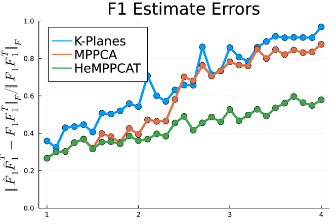
(a) $\bm{F}_{1}$ error vs. $v_{1}$

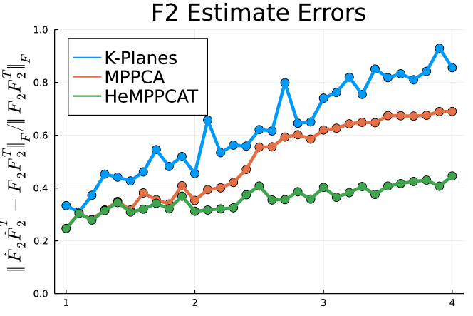
(b) $\bm{F}_{2}$ error vs. $v_{1}$

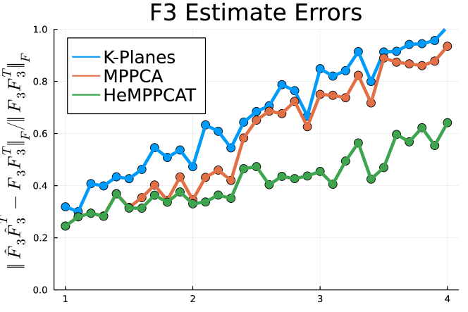
(c) $\bm{F}_{3}$ error vs. $v_{1}$

Fig. 1: Average $\bm{F}_{j}$ estimation error vs. $v_{1}$ (lower is better).

5.2 Hopkins 155 Dataset

In computer vision, motion segmentation is the task of segmenting moving objects in a video sequence into several independent regions, each corresponding to a different motion. The Hopkins 155 dataset is a series of 155 video sequences containing bodies in motion. The dataset has the coordinates of $n$ feature points $\bm{x}_{f,i}\in\mathbb{R}^{2}$ that were tracked across $F$ video frames. A feature point trajectory is formed by stacking the feature points across the frames: $\bm{y}_{i}=\begin{bmatrix}\bm{x}_{1,i}^{T}&\dots&\bm{x}_{F,i}^{T}\end{bmatrix}^{T}$. These trajectories are clustered to segment the motions using affine subspace clustering methods. A single body’s trajectories lie in an affine subspace with dimension of at most 4 [16], so the trajectories of $J$ bodies lie in a union of $J$ affine subspaces. The dataset includes the ground-truth cluster assignments for each trajectory.

Many motion segmentation methods assume the moving bodies are rigid. In practice, many common objects of interest do not satisfy rigid body motion. For instance, feature points on a walking human’s legs move with different velocities than feature points on the torso. These differences can be modeled as heteroscedastic noise: trajectories of the leg feature points may lie in a different noise group than those of the torso.

Each video sequence contains either $J=2$ or $J=3$ moving bodies. To simulate nonrigid body motion, we added synthetic Gaussian noise to the trajectories. In each sequence, we created $L=3$ synthetic noise groups with variances $v_{1},v_{2},v_{3}$ corresponding to signal to noise ratio (SNR) values of $-30,-25,$ and $-20$ dB relative to that sequence’s maximum trajectory $\ell_{2}$ norm. Noise groups 1, 2, and 3 contained 50%, 35%, and 15% of all trajectories, respectively.

For each sequence, we divided the dataset of trajectories into train and test sets using an 80/20 split. We applied K-Planes, MPPCA, and HeMPPCAT on the train set, and then used parameter estimates from all methods to classify trajectories in the test set. The test trajectories were classified based on nearest affine subspace using the K-Planes estimates, and by maximum likelihood using MPPCA and HeMPPCAT estimates, i.e., the predicted body for a test point $\bm{y}$ was $\operatorname{argmax}\limits_{j}\hat{\pi}_{j}p(\bm{y}\>|\>j;\hat{\bm{\theta}})$, where $\hat{\pi}_{j}$ is the estimated mixing proportion of body $j$. We computed $p(\bm{y}\>|\>j;\hat{\bm{\theta}})$ according to the approaches’ respective data models (1) and (3).

Table 1 shows the misclassification rate on the test set using the methods’ parameter estimates. Using HeMPPCAT’s estimates achieved lower classification error than using the other two approaches’ estimates in each of the noise groups, and on the overall test set.

K-Planes MPPCA HeMPPCAT Noise group 1 (low noise) 24.1% 19.4% 18.6% Noise group 2 (medium noise) 24.5% 27.3% 19.3% Noise group 3 (high noise) 28.0% 34.8% 20.1% Overall 24.8% 24.5% 19.1%

Table 1: Average misclassification rate on Hopkins 155 video dataset with synthetic heteroscedastic noise (lower is better).

6 Conclusion

This paper generalized MPPCA to jointly estimate the underlying factors, means, and noise variances from data with heteroscedastic noise. The proposed EM algorithm sequentially updates the mixing proportions, noise variances, means, and factor estimates. Experimental results on synthetic and the Hopkins 155 datasets illustrate the benefit of accounting for heteroscedastic noise.

There are several possible interesting directions for future work. We could generalize this approach even further by accounting for other cases of heterogeneity, e.g., missing data or heteroscedastic noise across features. There may be faster convergence variants of EM such as a space-alternating generalized EM (SAGE) approach [17] that could be explored. Another direction could be jointly estimating the number of noise groups $L$ and mixtures $J$ along with the other parameters.

Appendix A Complete-Data Log-Likelihood Expansion

We first compute the expression for $p(\bm{y}_{\ell,i},\bm{z}_{\ell ij})=p(\bm{y}_{\ell,i}\>|\>\bm{z}_{\ell ij})p(\bm{z}_{\ell ij})$. Given the coefficients $\bm{z}_{\ell ij}$, the only random component in sample $\bm{y}_{\ell,i}$ is due to the Gaussian noise vector $\bm{\epsilon}_{\ell,i}\sim\mathcal{N}(\bm{0}_{k},v_{\ell}\bm{I})$:

$$p(\bm{y}_{\ell,i}\>|\>\bm{z}_{\ell ij}) =(2\pi)^{-d/2}\mathrm{det}(v_{\ell}\bm{I})^{-1/2}\mathrm{exp}\Big{\{}-\frac{1}{2}(\bm{y}_{\ell,i}-\bm{F}_{j}\bm{z}_{\ell ij}-\bm{\mu}_{j})^{T}(v_{\ell}\bm{I})^{-1}(\bm{y}_{\ell,i}-\bm{F}_{J}\bm{z}_{\ell ij}-\bm{\mu}_{j})\Big{\}}$$ (9)

$$=(2\pi v_{\ell})^{-d/2}\mathrm{exp}\Big{\{}-\frac{1}{2v_{\ell}}\|\bm{y}_{\ell,i}-\bm{F}_{j}-\bm{z}_{\ell ij}\|_{2}^{2}\Big{\}}.$$ (10)

The coefficients $\bm{z}_{\ell ij}$ are assumed to be standard Gaussian vectors:

$$p(\bm{z}_{\ell ij}) =(2\pi)^{-k/2}\mathrm{det}(\bm{I})^{-1/2}\mathrm{exp}\Big{\{}-\frac{1}{2}\bm{z}_{\ell ij}^{T}\bm{I}^{-1}\bm{z}_{\ell ij}\Big{\}}$$ (11)

$$=(2\pi)^{-k/2}\mathrm{exp}\Big{\{}-\frac{1}{2}\bm{z}_{\ell ij}^{T}\bm{z}_{\ell ij}\Big{\}}.$$ (12)

Multiplying the two expressions above results in the following joint distribution:

$$p(\bm{y}_{\ell,i},\bm{z}_{\ell ij})=(2\pi v_{\ell})^{-d/2}\mathrm{exp}\Big{\{}-\frac{1}{2v_{\ell}}\|\bm{y}_{\ell,i}-\bm{F}_{j}\bm{z}_{\ell ij}-\bm{\mu}_{j}\|_{2}^{2}\Big{\}}(2\pi)^{-k/2}\mathrm{exp}\Big{\{}-\frac{1}{2}\bm{z}_{\ell ij}^{T}\bm{z}_{\ell ij}\Big{\}}.$$ (13)

Substituting (13) into (5) results in the following complete-data log-likelihood expression:

$$\mathcal{L} {}_{C}(\theta)=\sum_{\ell=1}^{L}\sum_{i=1}^{n_{\ell}}\sum_{j=1}^{J}g_{\ell ij}\bigg{\{}\mathrm{ln}\big{\{}\pi_{j}p(\bm{y}_{\ell,i},\bm{z}_{\ell ij})\big{\}}\bigg{\}}$$

$$=\sum_{\ell=1}^{L}\sum_{i=1}^{n_{\ell}}\sum_{j=1}^{J}g_{\ell ij}\bigg{\{}\mathrm{ln}(\pi_{j})+\mathrm{ln}\big{(}p(\bm{y}_{\ell,i},\bm{z}_{\ell ij})\big{)}\bigg{\}}$$

$$=\sum_{\ell=1}^{L}\sum_{i=1}^{n_{\ell}}\sum_{j=1}^{J}g_{\ell ij}\bigg{\{}\mathrm{ln}(\pi_{j})-\frac{d}{2}\mathrm{ln}(v_{\ell})-\frac{1}{2v_{\ell}}\|\bm{y}_{\ell,i}-\bm{F}_{j}\bm{z}_{\ell ij}-\bm{\mu}_{j}\|_{2}^{2}-\frac{1}{2}\bm{z}_{\ell ij}^{T}\bm{z}_{\ell ij}\bigg{\}}$$

$$=\sum_{\ell=1}^{L}\sum_{i=1}^{n_{\ell}}\sum_{j=1}^{J}g_{\ell ij}\bigg{\{}\mathrm{ln}(\pi_{j})-\frac{d}{2}\mathrm{ln}(v_{\ell})-\frac{1}{2v_{\ell}}(\bm{y}_{\ell,i}-\bm{F}_{j}\bm{z}_{\ell ij}-\bm{\mu}_{j})^{T}(\bm{y}_{\ell,i}-\bm{F}_{j}\bm{z}_{\ell ij}-\bm{\mu}_{j})-\frac{1}{2}\bm{z}_{\ell ij}^{T}\bm{z}_{\ell ij}\bigg{\}}$$

$$=\sum_{\ell=1}^{L}\sum_{i=1}^{n_{\ell}}\sum_{j=1}^{J}g_{\ell ij}\bigg{\{}\mathrm{ln}(\pi_{j})-\frac{d}{2}\mathrm{ln}(v_{\ell})-\frac{1}{2}\bm{z}_{\ell ij}^{T}\bm{z}_{\ell ij}-\frac{1}{2v_{\ell}}\|\bm{y}_{\ell,i}-\bm{\mu}_{j}\|_{2}^{2}+\frac{1}{v_{\ell}}\bm{z}_{\ell ij}^{T}\bm{F}^{T}_{j}(\bm{y}_{\ell,i}-\bm{\mu}_{j})-\frac{1}{2v_{\ell}}\bm{z}_{\ell ij}^{T}\bm{F}^{T}_{j}\bm{F}_{j}\bm{z}_{\ell ij}\bigg{\}}$$

$$=\sum_{\ell=1}^{L}\sum_{i=1}^{n_{\ell}}\sum_{j=1}^{J}g_{\ell ij}\bigg{\{}\mathrm{ln}(\pi_{j})-\frac{d}{2}\mathrm{ln}(v_{\ell})-\frac{1}{2}\mathrm{tr}(\bm{z}_{\ell ij}\bm{z}_{\ell ij}^{T})-\frac{1}{2v_{\ell}}\|\bm{y}_{\ell,i}-\bm{\mu}_{j}\|_{2}^{2}+\frac{1}{v_{\ell}}\bm{z}_{\ell ij}^{T}\bm{F}^{T}_{j}(\bm{y}_{\ell,i}-\bm{\mu}_{j})-\frac{1}{2v_{\ell}}\mathrm{tr}(\bm{F}^{T}_{j}\bm{F}_{j}\bm{z}_{\ell ij}\bm{z}_{\ell ij}^{T})\bigg{\}}.$$

We ignored the constant terms $-\frac{d}{2}\mathrm{ln}(2\pi)$ and $-\frac{k}{2}\mathrm{ln}(2\pi)$.

Appendix B Expectation Step Derivation

B.1 Product of Conditional Expectations

The E-Step of EM requires computing the expectation of (5) conditioned on the data samples $\bm{y}_{\ell,i}$ for $i=1,\dots,n_{\ell}$ and $\ell=1,\dots,L$. The expected value of $\mathcal{L}_{C}(\theta)$ given the samples is

$$\langle\mathcal{L}_{C}(\theta)\rangle=\sum_{\ell=1}^{L}\sum_{i=1}^{n_{\ell}}\sum_{j=1}^{J}\> \mathbb{E}\Bigg{[}g_{\ell ij}\mathrm{ln}(\pi_{j})-g_{\ell ij}\frac{d}{2}\mathrm{ln}(v_{\ell})-g_{\ell ij}\frac{1}{2}\mathrm{tr}(\bm{z}_{\ell ij}\bm{z}_{\ell ij}^{T})$$ (14)

$$-g_{\ell ij}\frac{1}{2v_{\ell}}\|\bm{y}_{\ell,i}-\bm{\mu}_{j}\|_{2}^{2}+g_{\ell ij}\frac{1}{v_{\ell}}\bm{z}_{\ell ij}^{T}\bm{F}^{T}_{j}(\bm{y}_{\ell,i}-\bm{\mu}_{j})-g_{\ell ij}\frac{1}{2v_{\ell}}\mathrm{tr}(\bm{F}^{T}_{j}\bm{F}_{j}\bm{z}_{\ell ij}\bm{z}_{\ell ij}^{T})\>\bigg{|}\>\bm{y}_{\ell,i}\Bigg{]}.$$

To simplify (14), we show $\mathbb{E}\big{[}g_{\ell ij}\bm{z}_{\ell ij}\>|\>\bm{y}_{\ell,i}\big{]}=\mathbb{E}\big{[}g_{\ell ij}\>|\>\bm{y}_{\ell,i}\big{]}\mathbb{E}\big{[}\bm{z}_{\ell ij}\>|\>g_{\ell ij}=1,\bm{y}_{\ell,i}\big{]}$ for all $i=1,\dots,n_{\ell}$, $\ell=1,\dots,L$, and $j=1,\dots,J$:

$$\mathbb{E}\Big{[} g_{\ell ij}\bm{z}_{\ell ij}\>|\>\bm{y}_{\ell,i}\Big{]}=\mathbb{E}\Big{[}g_{\ell ij}\mathbb{E}\big{[}\bm{z}_{\ell ij}\>|\>g_{\ell ij},\bm{y}_{\ell,i}\big{]}\big{|}\bm{y}_{\ell,i}\Big{]}$$

$$=\bigg{(}0*\mathbb{E}\Big{[}\bm{z}_{\ell ij}\>|\>g_{\ell ij}=0,\bm{y}_{\ell,i}\Big{]}*p(g_{\ell ij}=0\>|\>\bm{y}_{\ell,i})\bigg{)}+\bigg{(}1*\mathbb{E}\Big{[}\bm{z}_{\ell ij}\>|\>g_{\ell ij}=1,\bm{y}_{\ell,i}\Big{]}*p(g_{\ell ij}=1\>|\>\bm{y}_{\ell,i})\bigg{)}$$

$$=\mathbb{E}\Big{[}\bm{z}_{\ell ij}\>|\>g_{\ell ij}=1,\bm{y}_{\ell,i}\Big{]}\mathbb{E}\Big{[}g_{\ell ij}\>|\>\bm{y}_{\ell,i}\Big{]}.$$

Therefore:

$$\langle\mathcal{L}_{C}(\theta)\rangle=\sum_{\ell=1}^{L}\sum_{i=1}^{n_{\ell}}\sum_{j=1}^{J}\> \mathbb{E}\Big{[}g_{\ell ij}\>|\>\bm{y}_{\ell,i}\Big{]}\mathrm{ln}(\pi_{j})-\frac{d}{2}\mathbb{E}\Big{[}g_{\ell ij}\>|\>\bm{y}_{\ell,i}\Big{]}\mathrm{ln}(v_{\ell})-\frac{1}{2}\mathbb{E}\Big{[}g_{\ell ij}\>|\>\bm{y}_{\ell,i}\Big{]}\mathrm{tr}\Big{(}\mathbb{E}\big{[}\bm{z}_{\ell ij}\bm{z}_{\ell ij}^{T}\>|\>g_{\ell ij}=1,\bm{y}_{\ell,i}\big{]}\Big{)}$$

$$-\frac{1}{2v_{\ell}}\mathbb{E}\Big{[}g_{\ell ij}\>|\>\bm{y}_{\ell,i}\Big{]}\|\bm{y}_{\ell,i}-\bm{\mu}_{j}\|_{2}^{2}+\frac{1}{v_{\ell}}\mathbb{E}\Big{[}g_{\ell ij}\>|\>\bm{y}_{\ell,i}\Big{]}\mathbb{E}\Big{[}\bm{z}_{\ell ij}\>|\>g_{\ell ij}=1,\bm{y}_{\ell,i}\Big{]}^{T}\bm{F}^{T}_{j}(\bm{y}_{\ell,i}-\bm{\mu}_{j})$$

$$-\frac{1}{2v_{\ell}}\mathbb{E}\Big{[}g_{\ell ij}\>|\>\bm{y}_{\ell,i}\Big{]}\mathrm{tr}\Big{(}\bm{F}^{T}_{j}\bm{F}_{j}\mathbb{E}\big{[}\bm{z}_{\ell ij}\bm{z}_{\ell ij}^{T}\>|\>g_{\ell ij}=1,\bm{y}_{\ell,i}\big{]}\Big{)}.$$

Letting $R_{\ell ij}:=\mathbb{E}[g_{\ell ij}\>|\>\bm{y}_{\ell,i}]$, $\langle\bm{z}_{\ell ij}\rangle:=\mathbb{E}[\bm{z}_{\ell ij}\>|\>g_{\ell ij}=1,\bm{y}_{\ell,i}]$, and $\langle\bm{z}_{\ell ij}\bm{z}_{\ell ij}^{T}\rangle:=\mathbb{E}[\bm{z}_{\ell ij}\bm{z}_{\ell ij}^{T}\>|\>g_{\ell ij}=1,\bm{y}_{\ell,i}]$, the expected complete-data log-likelihood is

$$\langle\mathcal{L}_{C}(\theta)\rangle=\sum_{\ell=1}^{L}\sum_{i=1}^{n_{\ell}}\sum_{j=1}^{J} R_{\ell ij}\bigg{\{}\mathrm{ln}(\pi_{j})-\frac{d}{2}\mathrm{ln}(v_{\ell})-\frac{1}{2}\mathrm{tr}\Big{(}\langle\bm{z}_{\ell ij}\bm{z}_{\ell ij}^{T}\rangle\Big{)}$$

$$-\frac{1}{2v_{\ell}}\|\bm{y}_{\ell,i}-\bm{\mu}_{j}\|_{2}^{2}+\frac{1}{v_{\ell}}\langle\bm{z}_{\ell ij}\rangle^{T}\bm{F}^{T}_{j}(\bm{y}_{\ell,i}-\bm{\mu}_{j})$$

$$-\frac{1}{2v_{\ell}}\mathrm{tr}\Big{(}\bm{F}^{T}_{j}\bm{F}_{j}\langle\bm{z}_{\ell ij}\bm{z}_{\ell ij}^{T}\rangle\Big{)}\bigg{\}}.$$

B.2 Mixing Responsibilities

Since $g_{\ell ij}$ is a categorical random variable, the expectation $R_{\ell ij}$ is simply $p(g_{\ell ij}=1\>|\>\bm{y}_{\ell,i})$. This expression can be computed using Bayes’ rule:

$$R_{\ell ij}=\mathbb{E}[g_{\ell ij}\>|\>\bm{y}_{\ell,i}]=p(g_{\ell ij}=1\>|\>\bm{y}_{\ell,i})=\frac{p(\bm{y}_{\ell,i}\>|\>g_{\ell ij}=1)p(g_{\ell ij}=1)}{p(\bm{y}_{\ell,i})}=\frac{p(\bm{y}_{\ell,i}\>|\>j)\pi_{j}}{p(\bm{y}_{\ell,i})}.$$ (15)

B.3 Conditional Coefficent Expectation and Covariance

To derive $\langle\bm{z}_{\ell ij}\rangle$ and $\langle\bm{z}_{\ell ij}\bm{z}_{\ell ij}^{T}\rangle$, we first compute the conditional probability distribution $p(\bm{z}_{\ell ij}\>|\>g_{\ell ij}=1,\bm{y}_{\ell,i})$. This can again be done using Bayes’ rule:

$$p (\bm{z}_{\ell ij}\>|\>g_{\ell ij}=1,\bm{y}_{\ell,i})=\frac{p(\bm{y}_{\ell,i}\>|\>g_{\ell ij}=1,\bm{z}_{\ell ij})p(\bm{z}_{\ell ij}\>|\>g_{\ell ij}=1)}{p(\bm{y}_{\ell,i}\>|\>g_{\ell ij}=1)}$$

$$=\frac{(2\pi v_{\ell})^{-d/2}\mathrm{exp}\Big{\{}-\frac{1}{2v_{\ell}}\|\bm{y}_{\ell,i}-\bm{F}_{j}\bm{z}_{\ell ij}-\bm{\mu}_{j}\|_{2}^{2}\Big{\}}(2\pi)^{-k/2}\mathrm{exp}\Big{\{}-\frac{1}{2}\|\bm{z}_{\ell ij}\|_{2}^{2}\Big{\}}}{(2\pi)^{-d/2}\mathrm{det}(\bm{C}_{j})^{-1/2}\mathrm{exp}\Big{\{}-\frac{1}{2}(\bm{y}_{\ell,i}-\bm{\mu}_{j})^{T}\bm{C}_{\ell,j}^{-1}(\bm{y}_{\ell,i}-\bm{\mu}_{j})\Big{\}}}$$

$$=(2\pi)^{-k/2}v_{\ell}^{-d/2}\mathrm{det}(\bm{C}_{\ell,j})^{1/2}\mathrm{exp}\Big{\{}-\frac{1}{2v_{\ell}}\|\bm{y}_{\ell,i}-\bm{F}_{j}\bm{z}_{\ell ij}-\bm{\mu}_{j}\|_{2}^{2}-\frac{1}{2}\|\bm{z}_{\ell ij}\|_{2}^{2}+\frac{1}{2}(\bm{y}_{\ell,i}-\bm{\mu}_{j})^{T}\bm{C}_{\ell,j}^{-1}(\bm{y}_{\ell,i}-\bm{\mu}_{j})\Big{\}}.$$

The term $v_{\ell}^{-d/2}\mathrm{det}(\bm{C}_{\ell,j})^{1/2}$ can be simplified as such:

$$v_{\ell}^{-d/2} \mathrm{det}(\bm{C}_{\ell,j})^{1/2}=\Big{(}v_{\ell}^{-d}\mathrm{det}(\bm{C}_{\ell,j})\Big{)}^{1/2}$$

$$=\Big{(}v_{\ell}^{-d}\mathrm{det}(\bm{F}_{j}\bm{F}^{T}_{j}+v_{\ell}\bm{I}_{d})\Big{)}^{1/2}$$

$$=\Big{(}v_{\ell}^{-d}\mathrm{det}\big{(}\bm{I}_{k}+\bm{F}^{T}_{j}(v_{\ell}\bm{I}_{d})^{-1}\bm{F}_{j}\big{)}\mathrm{det}(v_{\ell}\bm{I}_{d})\Big{)}^{1/2}$$

$$=\Big{(}v_{\ell}^{-d}\mathrm{det}\big{(}\bm{I}_{k}+v_{\ell}^{-1}\bm{F}^{T}_{j}\bm{F}_{j}\big{)}v_{\ell}^{d}\Big{)}^{1/2}$$

$$=\mathrm{det}\big{(}v_{\ell}^{-1}(v_{\ell}\bm{I}_{k}+\bm{F}^{T}_{j}\bm{F}_{j})\big{)}^{1/2}$$

$$=\mathrm{det}\big{(}v_{\ell}^{-1}\bm{M}_{\ell,j}\big{)}^{1/2}=\mathrm{det}\big{(}v_{\ell}\bm{M}_{\ell,j}^{-1}\big{)}^{-1/2}.$$

The term inside the $\mathrm{exp}(\cdot)$ can also be simplified as such. Let $\bar{\bm{y}}_{\ell ij}:=(\bm{y}_{\ell,i}-\bm{\mu}_{j})$:

$$-\frac{1}{2v_{\ell}} \|\bar{\bm{y}}_{\ell ij}-\bm{F}_{j}\bm{z}_{\ell ij}\|_{2}^{2}-\frac{1}{2}\|\bm{z}_{\ell ij}\|_{2}^{2}+\frac{1}{2}\bar{\bm{y}}_{\ell ij}^{T}\bm{C}_{\ell,j}^{-1}\bar{\bm{y}}_{\ell ij}$$

$$=-\frac{1}{2v_{\ell}}(\bar{\bm{y}}_{\ell ij}-\bm{F}_{j}\bm{z}_{\ell ij})^{T}(\bar{\bm{y}}_{\ell ij}-\bm{F}_{j}\bm{z}_{\ell ij})-\frac{1}{2}\bm{z}_{\ell ij}^{T}\bm{z}_{\ell ij}+\frac{1}{2}\bar{\bm{y}}_{\ell ij}^{T}\bm{C}_{\ell,j}^{-1}\bar{\bm{y}}_{\ell ij}$$

$$=-\frac{1}{2v_{\ell}}\bigg{[}\bar{\bm{y}}_{\ell ij}^{T}\bar{\bm{y}}_{\ell ij}-\bar{\bm{y}}_{\ell ij}^{T}\bm{F}_{j}\bm{z}_{\ell ij}-\bm{z}_{\ell ij}^{T}\bm{F}^{T}_{j}\bar{\bm{y}}_{\ell ij}+\bm{z}_{\ell ij}^{T}\bm{F}^{T}_{j}\bm{F}_{j}\bm{z}_{\ell ij}+v_{\ell}\bm{z}_{\ell ij}^{T}\bm{z}_{\ell ij}-v_{\ell}\bar{\bm{y}}_{\ell ij}^{T}\bm{C}_{\ell,j}^{-1}\bar{\bm{y}}_{\ell ij}\bigg{]}$$

$$=-\frac{1}{2v_{\ell}}\bigg{[}\bar{\bm{y}}_{\ell ij}^{T}\bar{\bm{y}}_{\ell ij}-\bar{\bm{y}}_{\ell ij}^{T}\bm{F}_{j}\bm{z}_{\ell ij}-\bm{z}_{\ell ij}^{T}\bm{F}^{T}_{j}\bar{\bm{y}}_{\ell ij}+\bm{z}_{\ell ij}^{T}\bm{F}^{T}_{j}\bm{F}_{j}\bm{z}_{\ell ij}+v_{\ell}\bm{z}_{\ell ij}^{T}\bm{z}_{\ell ij}-\bar{\bm{y}}_{\ell ij}^{T}(\bm{I}_{d}-\bm{F}_{j}\bm{M}_{\ell,j}^{-1}\bm{F}^{T}_{j})\bar{\bm{y}}_{\ell ij}\bigg{]}$$

$$=-\frac{1}{2v_{\ell}}\bigg{[}\bar{\bm{y}}_{\ell ij}^{T}(\bm{F}_{j}\bm{M}_{\ell,j}^{-1}\bm{F}^{T}_{j})\bar{\bm{y}}_{\ell ij}-\bar{\bm{y}}_{\ell ij}^{T}\bm{F}_{j}\bm{z}_{\ell ij}-\bm{z}_{\ell ij}^{T}\bm{F}^{T}_{j}\bar{\bm{y}}_{\ell ij}+\bm{z}_{\ell ij}^{T}\bm{M}_{\ell,j}\bm{z}_{\ell ij}\bigg{]}$$

$$=-\frac{1}{2v_{\ell}}\bigg{[}\bm{z}_{\ell ij}^{T}\bm{M}_{\ell,j}\bm{z}_{\ell ij}-\bm{z}_{\ell ij}^{T}\bm{F}^{T}_{j}\bar{\bm{y}}_{\ell ij}-\bar{\bm{y}}_{\ell ij}^{T}\bm{F}_{j}\bm{M}_{\ell,j}^{-1}\bm{M}_{\ell,j}\bm{z}_{\ell ij}+\bar{\bm{y}}_{\ell ij}^{T}(\bm{F}_{j}\bm{M}_{\ell,j}^{-1}\bm{F}^{T}_{j})\bar{\bm{y}}_{\ell ij}\bigg{]}$$

$$=-\frac{1}{2v_{\ell}}\bigg{[}(\bm{z}_{\ell ij}-\bm{M}_{\ell,j}^{-1}\bm{F}_{j}\bar{\bm{y}}_{\ell ij})^{T}\bm{M}_{\ell,j}(\bm{z}_{\ell ij}-\bm{M}_{\ell,j}^{-1}\bm{F}_{j}\bar{\bm{y}}_{\ell ij})\bigg{]}$$

$$=-\frac{1}{2}\bigg{[}(\bm{z}_{\ell ij}-\bm{M}_{\ell,j}^{-1}\bm{F}_{j}\bar{\bm{y}}_{\ell ij})^{T}(v_{\ell}\bm{M}_{\ell,j}^{-1})^{-1}(\bm{z}_{\ell ij}-\bm{M}_{\ell,j}^{-1}\bm{F}_{j}\bar{\bm{y}}_{\ell ij})\bigg{]},$$

where $\bm{C}_{\ell,j}^{-1}=v_{\ell}^{-1}(\bm{I}_{d}-\bm{F}_{j}\bm{M}_{\ell,j}^{-1}\bm{F}^{T}_{j})$ is derived using the Matrix-Inversion Lemma.

The conditional probability distribution $p(\bm{z}_{\ell ij}\>|\>g_{\ell ij}=1,\bm{y}_{\ell,i})$ is equal to

$$(2\pi)^{-k/2}\mathrm{det}(v_{\ell}\bm{M}_{\ell,j}^{-1})^{-1/2}\mathrm{exp}\Big{(}-\frac{1}{2}(\bm{z}_{\ell ij}-\bm{M}_{\ell,j}^{-1}\bm{F}_{j}\bar{\bm{y}}_{\ell ij})^{T}(v_{\ell}\bm{M}_{\ell,j}^{-1})^{-1}(\bm{z}_{\ell ij}-\bm{M}_{\ell,j}^{-1}\bm{F}_{j}\bar{\bm{y}}_{\ell ij})\Big{)}$$ (16)

which is a Gaussian distribution with mean $\bm{M}_{\ell,j}^{-1}\bm{F}_{j}(\bm{y}_{\ell,i}-\bm{\mu}_{j})$ and covariance $v_{\ell}\bm{M}_{\ell,j}^{-1}$.

The conditional expectation $\langle\bm{z}_{\ell ij}\rangle$ is therefore $\bm{M}_{\ell,j}^{-1}\bm{F}_{j}(\bm{y}_{\ell,i}-\bm{\mu}_{j})$. The term $\langle\bm{z}_{\ell ij}\bm{z}_{\ell ij}^{T}\rangle$ can be derived as follows:

$$v_{\ell}\bm{M}_{\ell,j}^{-1} =\mathbb{E}[(\bm{z}_{\ell ij}-\langle\bm{z}_{\ell ij}\rangle)(\bm{z}_{\ell ij}-\langle\bm{z}_{\ell ij}\rangle)^{T}\>|\>g_{\ell ij}=1,\bm{y}_{\ell,i}]$$

$$=\mathbb{E}[\bm{z}_{\ell ij}\bm{z}_{\ell ij}^{T}\>|\>g_{\ell ij}=1,\bm{y}_{\ell,i}]-\mathbb{E}[\bm{z}_{\ell ij}\>|\>g_{\ell ij}=1,\bm{y}_{\ell,i}]\>\mathbb{E}[\bm{z}_{\ell ij}\>|\>g_{\ell ij}=1,\bm{y}_{\ell,i}]^{T}$$

$$=\langle\bm{z}_{\ell ij}\bm{z}_{\ell ij}^{T}\rangle-\langle\bm{z}_{\ell ij}\rangle\langle\bm{z}_{\ell ij}\rangle^{T}$$

$$\langle\bm{z}_{\ell ij}\bm{z}_{\ell ij}^{T}\rangle =v_{\ell}\bm{M}_{\ell,j}^{-1}+\langle\bm{z}_{\ell ij}\rangle\langle\bm{z}_{\ell ij}\rangle^{T}.$$ (17)

B.4 Final E-Step Computation

The final expected complete data log-likelihood is

$$\langle\mathcal{L}_{C}(\theta;\theta^{(t)})\rangle=\sum_{\ell=1}^{L}\sum_{i=1}^{n_{\ell}}\sum_{j=1}^{J} R_{\ell ij}^{(t)}\bigg{\{}\mathrm{ln}(\pi_{j})-\frac{d}{2}\mathrm{ln}(v_{\ell})-\frac{1}{2}\mathrm{tr}\Big{(}\langle\bm{z}_{\ell ij}\bm{z}_{\ell ij}^{T}\rangle\Big{)}$$ (18)

$$-\frac{1}{2v_{\ell}}\|\bm{y}_{\ell,i}-\bm{\mu}_{j}\|_{2}^{2}+\frac{1}{v_{\ell}}\langle\bm{z}_{\ell ij}\rangle^{T}\bm{F}^{T}_{j}(\bm{y}_{\ell,i}-\bm{\mu}_{j})$$

$$-\frac{1}{2v_{\ell}}\mathrm{tr}\Big{(}\bm{F}^{T}_{j}\bm{F}_{j}\langle\bm{z}_{\ell ij}\bm{z}_{\ell ij}^{T}\rangle\Big{)}\bigg{\}},$$

where the conditional expectations are computed using the current EM iterate’s parameter estimates:

$$\begin{gathered}\langle\bm{z}_{\ell ij}\rangle=\bm{M}_{\ell,j}^{(t)\>-1}\bm{F}^{(t)\>T}_{j}(\bm{y}_{\ell,i}-\bm{\mu}_{j}^{(t)})\\ \langle\bm{z}_{\ell ij}\bm{z}_{\ell ij}^{T}\rangle=v^{(t)}_{\ell}\bm{M}_{\ell,j}^{(t)\>-1}+\langle\bm{z}_{\ell ij}\rangle\langle\bm{z}_{\ell ij}\rangle^{T}\\ \bm{M}_{\ell,j}^{(t)}=v^{(t)}_{\ell}\bm{I}_{k}+\bm{F}^{(t)\>T}_{j}\bm{F}^{(t)}_{j}.\end{gathered}$$ (19)

Appendix C Maximization Step Derivation

C.1 Mixing Proportions

We derive the update expression for each mixing proportion $\pi_{j}$ by maximizing (18) with respect to $\pi_{j}$ subject to the constraint $\sum\limits_{j=1}^{J}\pi_{j}=1$. This is equivalent to maximizing

$$\sum\limits_{j=1}^{J}\sum\limits_{\ell=1}^{L}\sum\limits_{i=1}^{n_{\ell}}R_{\ell ij}^{(t)}\mathrm{ln}(\pi_{j})$$ (20)

subject to the same constraint. To account for this constraint, we introduce the Lagrange multiplier $\lambda$. Let $f_{1}:=\sum\limits_{j=1}^{J}R_{j}\mathrm{ln}(\pi_{j})+\lambda\Big{(}\sum\limits_{j=1}^{J}\pi_{j}-1\Big{)}$. Suppose we choose an arbitrary $j\in\{1,\dots,J\}$. We first calculate an expression for $\pi_{j}^{(t+1)}$ in terms of $\lambda$:

$$\begin{gathered}\frac{\partial f_{1}}{\partial\pi_{j}}=\frac{\sum\limits_{\ell=1}^{L}\sum\limits_{i=1}^{n_{\ell}}R_{\ell ij}^{(t)}}{\pi_{j}}+\lambda,\\ \frac{\sum\limits_{\ell=1}^{L}\sum\limits_{i=1}^{n_{\ell}}R_{\ell ij}^{(t)}}{\pi_{j}^{(t+1)}}+\lambda=0,\\ \pi_{j}^{(t+1)}=-\frac{\sum\limits_{\ell=1}^{L}\sum\limits_{i=1}^{n_{\ell}}R_{\ell ij}^{(t)}}{\lambda}.\end{gathered}$$

We then use the constraint function to find an expression for $\lambda$ in terms of $R_{\ell ij}^{(t)}$, and use that to calculate the final expression for $\pi_{j}^{(t+1)}$:

$$\begin{gathered}\sum\limits_{j=1}^{J}\pi_{j}^{(t+1)}=-\sum\limits_{j=1}^{J}\frac{\sum\limits_{\ell=1}^{L}\sum\limits_{i=1}^{n_{\ell}}R_{\ell ij}^{(t)}}{\lambda}=1,\\ \lambda=-\sum\limits_{j=1}^{J}\sum\limits_{\ell=1}^{L}\sum\limits_{i=1}^{n_{\ell}}R_{\ell ij}^{(t)}=-n,\\ \pi_{j}^{(t+1)}=\frac{\sum\limits_{\ell=1}^{L}\sum\limits_{i=1}^{n_{\ell}}R_{\ell ij}^{(t)}}{n}.\end{gathered}$$

This matches the update expression in Section 4.2 and holds for all $j\in\{1,\dots,J\}$.

C.2 Noise Variance

Deriving the update expression for each variance $v_{\ell}$ is equivalent to maximizing

$$f_{2}=\sum_{\ell=1}^{L}\sum_{i=1}^{n_{\ell}}\sum_{j=1}^{J}R_{\ell ij}\bigg{\{}-\frac{d}{2}\mathrm{ln}(v_{\ell})-\frac{1}{2v_{\ell}}\|\bm{y}_{\ell,i}-\bm{\mu}\|_{2}^{2}+\frac{1}{v_{\ell}}\langle\bm{z}_{\ell ij}\rangle^{T}\bm{F}^{T}_{j}(\bm{y}_{\ell,i}-\bm{\mu})-\frac{1}{2v_{\ell}}\mathrm{tr}(\bm{F}^{T}_{j}\bm{F}_{j}\langle\bm{z}_{\ell ij}\bm{z}_{\ell ij}^{T}\rangle)\bigg{\}}$$ (21)

with respect to $v_{\ell}$. Choosing an arbitrary $\ell\in\{1,\dots,L\}$:

$$\begin{gathered}\frac{\partial f_{2}}{\partial v_{\ell}}=\sum\limits_{i=1}^{n_{\ell}}\sum\limits_{j=1}^{J}R_{\ell ij}^{(t)}\bigg{\{}-\frac{d}{2v_{\ell}}+\frac{1}{2v_{\ell}^{2}}\|\bm{y}_{\ell,i}\|_{2}^{2}-\frac{1}{v_{\ell}^{2}}\langle\bm{z}_{\ell ij}\rangle^{T}\bm{F}^{T}_{j}(\bm{y}_{\ell,i}-\bm{\mu}_{j})+\frac{1}{2v_{\ell}^{2}}\mathrm{tr}(\bm{F}^{T}_{j}\bm{F}_{j}\langle\bm{z}_{\ell ij}\bm{z}_{\ell ij}^{T}\rangle)\bigg{\}},\\ \frac{1}{v^{(t+1)}_{\ell}}\sum\limits_{i=1}^{n_{\ell}}\sum\limits_{j=1}^{J}R_{\ell ij}\bigg{\{}-\frac{d}{2}+\frac{1}{2v^{(t+1)}_{\ell}}\|\bm{y}_{\ell,i}-\bm{\mu}_{j}\|_{2}^{2}-\frac{1}{v^{(t+1)}_{\ell}}\langle\bm{z}_{\ell ij}\rangle^{T}\bm{F}^{T}_{j}(\bm{y}_{\ell,i}-\bm{\mu}_{j})+\frac{1}{2v^{(t+1)}_{\ell}}\mathrm{tr}(\bm{F}^{T}_{j}\bm{F}_{j}\langle\bm{z}_{\ell ij}\bm{z}_{\ell ij}^{T}\rangle)\bigg{\}}=0,\\ \sum\limits_{i=1}^{n_{\ell}}\sum\limits_{j=1}^{J}R_{\ell ij}^{(t)}\bigg{\{}-\frac{d}{2}+\frac{1}{2v^{(t+1)}_{\ell}}\|\bm{y}_{\ell,i}-\bm{\mu}_{j}\|_{2}^{2}-\frac{1}{v^{(t+1)}_{\ell}}\langle\bm{z}_{\ell ij}\rangle^{T}\bm{F}^{T}_{j}(\bm{y}_{\ell,i}-\bm{\mu}_{j})+\frac{1}{2v^{(t+1)}_{\ell}}\mathrm{tr}(\bm{F}^{T}_{j}\bm{F}_{j}\langle\bm{z}_{\ell ij}\bm{z}_{\ell ij}^{T}\rangle)\bigg{\}}=0,\\ \frac{1}{v^{(t+1)}_{\ell}}\sum\limits_{i=1}^{n_{\ell}}\sum\limits_{j=1}^{J}R_{\ell ij}\bigg{\{}\frac{1}{2}\|\bm{y}_{\ell,i}-\bm{\mu}_{j}\|_{2}^{2}-\langle\bm{z}_{\ell ij}\rangle^{T}\bm{F}^{T}_{j}(\bm{y}_{\ell,i}-\bm{\mu}_{j})+\frac{1}{2}\mathrm{tr}(\bm{F}^{T}_{j}\bm{F}_{j}\langle\bm{z}_{\ell ij}\bm{z}_{\ell ij}^{T}\rangle)\bigg{\}}=\frac{d}{2}\sum\limits_{i=1}^{n_{\ell}}\sum\limits_{j=1}^{J}R_{\ell ij}^{(t)},\\ v^{(t+1)}_{\ell}=\frac{1}{d\sum\limits_{i=1}^{n_{\ell}}\sum\limits_{j=1}^{J}R_{\ell ij}^{(t)}}\Bigg{[}\sum\limits_{i=1}^{n_{\ell}}\sum\limits_{j=1}^{J}R_{\ell ij}\bigg{\{}\|\bm{y}_{\ell,i}-\bm{\mu}_{j}\|_{2}^{2}-2\langle\bm{z}_{\ell ij}\rangle^{T}\bm{F}^{T}_{j}(\bm{y}_{\ell,i}-\bm{\mu}_{j})+\mathrm{tr}(\bm{F}^{T}_{j}\bm{F}_{j}\langle\bm{z}_{\ell ij}\bm{z}_{\ell ij}^{T}\rangle)\bigg{\}}\Bigg{]}.\end{gathered}$$

This holds for all $\ell\in\{1,\dots,L\}$. Using the current iterate’s estimates $\bm{\mu}_{j}^{(t)}$ and $\bm{F}^{(t)}_{j}$ for $\bm{\mu}_{j}$ and $\bm{F}_{j}$, respectively, makes the expression match the corresponding equation in Section 4.2.

C.3 Means

Deriving the update expression for each mean $\bm{\mu}_{j}$ is equivalent to maximizing

$$f_{3}=\sum\limits_{j=1}^{J}\sum\limits_{\ell=1}^{L}\sum\limits_{i=1}^{n_{\ell}}R_{\ell ij}\bigg{\{}-\frac{1}{2v_{\ell}}\|\bm{y}_{\ell,i}-\bm{\mu}\|_{2}^{2}+\frac{1}{v_{\ell}}\langle\bm{z}_{\ell ij}\rangle^{T}\bm{F}^{T}_{j}(\bm{y}_{\ell,i}-\bm{\mu})\bigg{\}}$$ (22)

with respect to $\bm{\mu}_{j}$. Choosing an arbitrary $j\in\{1,\dots,J\}$:

$$\begin{gathered}\nabla_{\bm{\mu}_{j}}f_{3}=\sum\limits_{\ell=1}^{L}\sum\limits_{i=1}^{n_{\ell}}\frac{R_{\ell ij}}{v_{\ell}}\bigg{\{}\bm{y}_{\ell,i}-\bm{\mu}_{j}-\bm{F}_{j}\bm{z}_{\ell ij}\bigg{\}},\\ \sum\limits_{\ell=1}^{L}\sum\limits_{i=1}^{n_{\ell}}\frac{R_{\ell ij}}{v_{\ell}}\bigg{\{}\bm{y}_{\ell,i}-\bm{\mu}_{j}^{(t+1)}-\bm{F}_{j}\bm{z}_{\ell ij}\bigg{\}}=0,\\ \bm{\mu}_{j}^{(t+1)}=\frac{\sum\limits_{\ell=1}^{L}\sum\limits_{i=1}^{n_{\ell}}\frac{R_{\ell ij}^{(t)}}{v_{\ell}}[\bm{y}_{\ell,i}-\bm{F}_{j}\langle\bm{z}_{\ell ij}\rangle]}{\sum\limits_{\ell=1}^{L}\sum\limits_{i=1}^{n_{\ell}}\frac{R_{\ell ij}^{(t)}}{v_{\ell}}}.\end{gathered}$$

This holds for all $j\in\{1,\dots,J\}$. Using the current iterate’s estimate $\bm{F}_{j}^{(t)}$ for $\bm{F}_{j}$, and the new estimate $v^{(t+1)}_{\ell}$ for $v_{\ell}$, makes the expression match the corresponding equation in Section 4.2.

C.4 Factor Matrices

Deriving the update expression for each factor matrix $\bm{F}_{j}$ is equivalent to maximizing

$$f_{4}=\sum\limits_{j=1}^{J}\sum\limits_{\ell=1}^{L}\sum\limits_{i=1}^{n_{\ell}}R_{\ell ij}\bigg{\{}\frac{1}{v_{\ell}}\langle\bm{z}_{\ell ij}\rangle^{T}\bm{F}^{T}_{j}(\bm{y}_{\ell,i}-\bm{\mu})-\frac{1}{2v_{\ell}}\mathrm{tr}(\bm{F}^{T}_{j}\bm{F}_{j}\langle\bm{z}_{\ell ij}\bm{z}_{\ell ij}^{T}\rangle)\bigg{\}}$$ (23)

with respect to $\bm{F}_{j}$. Choosing an arbitrary $j\in\{1,\dots,J\}$:

$$f_{4} =\sum\limits_{\ell=1}^{L}\sum\limits_{i=1}^{n_{\ell}}R_{\ell ij}^{(t)}\bigg{\{}\frac{1}{v_{\ell}}\langle\bm{z}_{\ell ij}\rangle^{T}\bm{F}^{T}_{j}(\bm{y}_{\ell,i}-\bm{\mu})-\frac{1}{2v_{\ell}}\mathrm{tr}(\bm{F}^{T}_{j}\bm{F}_{j}\langle\bm{z}_{\ell ij}\bm{z}_{\ell ij}^{T}\rangle)\bigg{\}}$$

$$=\sum\limits_{\ell=1}^{L}\sum\limits_{i=1}^{n_{\ell}}\frac{R_{\ell ij}^{(t)}}{v_{\ell}}\bigg{\{}\mathrm{tr}\Big{(}(\bm{y}_{\ell,i}-\bm{\mu}_{j})^{T}\bm{F}_{j}\langle\bm{z}_{\ell ij}\rangle\Big{)}-\mathrm{tr}(\bm{F}^{T}_{j}\bm{F}_{j}\langle\bm{z}_{\ell ij}\bm{z}_{\ell ij}^{T}\rangle)\bigg{\}}$$

$$=\sum\limits_{\ell=1}^{L}\sum\limits_{i=1}^{n_{\ell}}\frac{R_{\ell ij}^{(t)}}{v_{\ell}}\bigg{\{}\mathrm{tr}\Big{(}\bm{F}_{j}\langle\bm{z}_{\ell ij}\rangle(\bm{y}_{\ell,i}-\bm{\mu}_{j})^{T}\Big{)}-\mathrm{tr}(\bm{F}_{j}\langle\bm{z}_{\ell ij}\bm{z}_{\ell ij}^{T}\rangle\bm{F}^{T}_{j})\bigg{\}}$$

$$=\mathrm{tr}\Bigg{(}\sum\limits_{\ell=1}^{L}\sum\limits_{i=1}^{n_{\ell}}\frac{R_{\ell ij}^{(t)}}{v_{\ell}}\bm{F}_{j}\langle\bm{z}_{\ell ij}\rangle(\bm{y}_{\ell,i}-\bm{\mu}_{j})^{T}-\sum\limits_{\ell=1}^{L}\sum\limits_{i=1}^{n_{\ell}}\frac{R_{\ell ij}^{(t)}}{v_{\ell}}\bm{F}_{j}\langle\bm{z}_{\ell ij}\bm{z}_{\ell ij}^{T}\rangle\bm{F}^{T}_{j}\Bigg{)}$$

$$=\mathrm{tr}\Bigg{(}\bm{F}_{j}\sum\limits_{\ell=1}^{L}\sum\limits_{i=1}^{n_{\ell}}\frac{R_{\ell ij}^{(t)}}{v_{\ell}}\langle\bm{z}_{\ell ij}\rangle(\bm{y}_{\ell,i}-\bm{\mu}_{j})^{T}-\frac{1}{2}\bm{F}_{j}\sum\limits_{\ell=1}^{L}\sum\limits_{i=1}^{n_{\ell}}\frac{R_{\ell ij}^{(t)}}{v_{\ell}}\langle\bm{z}_{\ell ij}\bm{z}_{\ell ij}^{T}\rangle\bm{F}^{T}_{j}\Bigg{)}.$$

Let $\bm{B}_{j}:=\sum\limits_{\ell=1}^{L}\sum\limits_{i=1}^{n_{\ell}}\frac{R_{\ell ij}^{(t)}}{v_{\ell}}\langle\bm{z}_{\ell ij}\rangle(\bm{y}_{\ell,i}-\bm{\mu}_{j})^{T}$ and $\bm{K}_{j}:=\sum\limits_{\ell=1}^{L}\sum\limits_{i=1}^{n_{\ell}}\frac{R_{\ell ij}^{(t)}}{v_{\ell}}\langle\bm{z}_{\ell ij}\bm{z}_{\ell ij}^{T}\rangle$.

$$f_{4} =\mathrm{tr}\big{(}\bm{F}_{j}\bm{B}_{j}-\frac{1}{2}\bm{F}_{j}\bm{K}_{j}\bm{F}^{T}_{j}\big{)}$$

$$=\mathrm{tr}\big{(}\bm{F}_{j}\bm{K}_{j}^{1/2}\bm{K}_{j}^{-1/2}\bm{B}_{j}-\frac{1}{2}\bm{F}_{j}\bm{K}_{j}^{1/2}\bm{K}_{j}^{1/2}\bm{F}^{T}_{j}\big{)},$$

where $\bm{A}^{1/2}$ denotes the principal square root of a positive semidefinite matrix $\bm{A}$, and $\bm{A}^{-1/2}$ denotes the inverse $\bm{A}^{1/2}$ if it is positive definite. Now let $\bm{X}_{j}=\bm{F}_{j}\bm{K}_{j}^{1/2}$ and $\tilde{\bm{B}}_{j}=\bm{K}_{j}^{-1/2}\bm{B}_{j}$.

$$\begin{gathered}f_{4}=\mathrm{tr}\big{(}\bm{X}_{j}\tilde{\bm{B}}_{j}-\frac{1}{2}\bm{X}_{j}\bm{X}_{j}^{T}\big{)},\\ \nabla_{\bm{X}_{j}}f_{4}=\tilde{\bm{B}}_{j}-\bm{X}_{j},\\ \tilde{\bm{B}}_{j}-\hat{\bm{X}}_{j}=0,\\ \bm{F}^{(t+1)}_{j}\bm{K}_{j}^{1/2}=\bm{B}_{j}^{T}\bm{K}_{j}^{-1/2},\\ \bm{F}^{(t+1)}_{j}=\bm{B}_{j}^{T}\bm{K}_{j}^{-1}=\bigg{[}\sum\limits_{\ell=1}^{L}\sum\limits_{i=1}^{n_{\ell}}\frac{R_{\ell ij}^{(t)}}{v_{\ell}}(\bm{y}_{\ell,i}-\bm{\mu}_{j})\langle\bm{z}_{\ell ij}\rangle^{T}\bigg{]}\bigg{[}\sum\limits_{\ell=1}^{L}\sum\limits_{i=1}^{n_{\ell}}\frac{R_{\ell ij}^{(t)}}{v_{\ell}}\langle\bm{z}_{\ell ij}\bm{z}_{\ell ij}^{T}\rangle\bigg{]}^{-1}.\end{gathered}$$

This holds for all $j\in\{1,\dots,J\}$. Using the new estimates $v^{(t+1)}_{\ell}$ and $\bm{\mu}_{j}^{(t+1)}$ for $v_{\ell}$ and $\bm{\mu}_{j}$, respectively, makes this expression match the corresponding equation in Section 4.2.

Appendix D Additional Simulation Results

We repeated the synthetic dataset experiments as described in Section 5, but initialized K-Planes, MPPCA, and HeMPPCAT using K-Means++. Figure D2 compares the average $\bm{F}_{j}$ estimation errors across the 25 datasets against $v_{1}$. Again, MPPCA and HeMPPCAT had similar estimation errors at lower values of $v_{1}$, but HeMPPCAT had much lower errors than MPPCA at larger values of $v_{1}$. Additionally, the non-statistical K-Planes mostly had higher errors than MPPCA and HeMPPCAT.

(a) $\bm{F}_{1}$ error vs. $v_{1}$

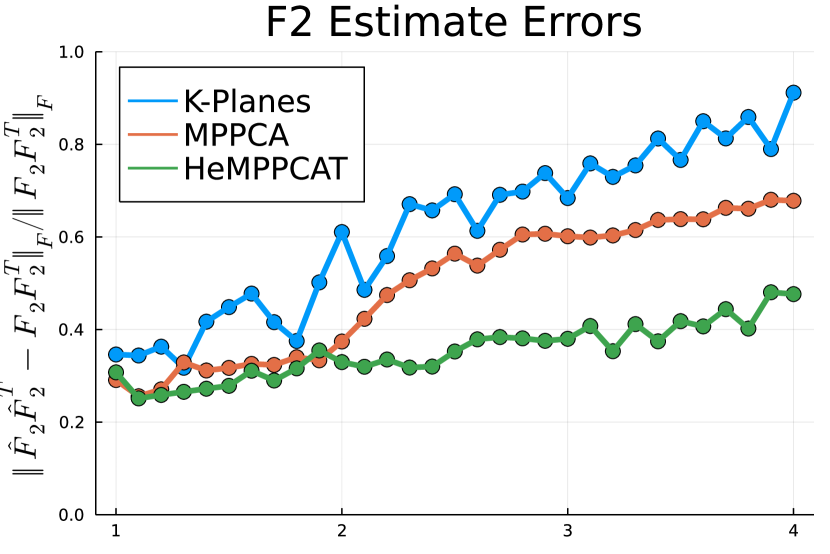
(b) $\bm{F}_{2}$ error vs. $v_{1}$

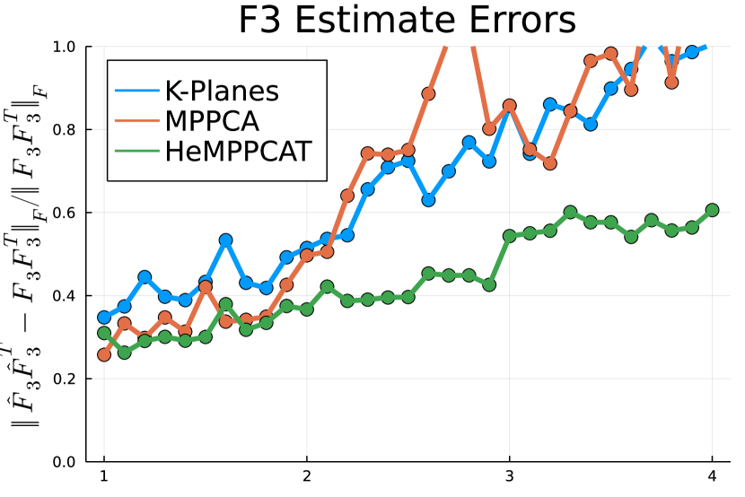
(c) $\bm{F}_{3}$ error vs. $v_{1}$

Fig. D2: Average $\bm{F}_{j}$ estimation error vs. variance $v_{1}$.

References

- [1] M. E. Tipping and C. M. Bishop, “Mixtures of probabilistic principal component analyzers,” Neural Computation, vol. 11, no. 2, pp. 443–82, Feb. 1999.
- [2] Y. M. Lu and M. N. Do, “Sampling signals from a union of subspaces [A new perspective for the extension of this theory],” IEEE Sig. Proc. Mag., vol. 25, no. 2, pp. 41–7, Mar. 2008.
- [3] T. Blumensath, “Sampling and reconstructing signals from a union of linear subspaces,” IEEE Trans. Info. Theory, vol. 57, no. 7, pp. 4660–71, July 2011.
- [4] Y. C. Eldar and M. Mishali, “Robust recovery of signals from a structured union of subspaces,” IEEE Trans. Info. Theory, vol. 55, no. 11, pp. 5302–16, Nov. 2009.
- [5] R. Vidal, Y. Ma, and S. Sastry, “Generalized principal component analysis (GPCA),” IEEE Trans. Patt. Anal. Mach. Int., vol. 27, no. 12, pp. 1945–59, Dec. 2005.
- [6] R. Vidal, “Subspace clustering,” IEEE Sig. Proc. Mag., vol. 28, no. 2, pp. 52–68, Mar. 2011.
- [7] Adnane Cabani, Karim Hammoudi, Halim Benhabiles, and Mahmoud Melkemi, “Maskedface-net–a dataset of correctly/incorrectly masked face images in the context of covid-19,” Smart Health, vol. 19, pp. 100144, 2021.
- [8] Athinodoros S. Georghiades, Peter N. Belhumeur, and David J. Kriegman, “From few to many: Illumination cone models for face recognition under variable lighting and pose,” IEEE transactions on pattern analysis and machine intelligence, vol. 23, no. 6, pp. 643–660, 2001.
- [9] D. Hong, K. Gilman, L. Balzano, and J. A. Fessler, “HePPCAT: probabilistic PCA for data with heteroscedastic noise,” IEEE Trans. Sig. Proc., vol. 69, pp. 4819–34, Aug. 2021.
- [10] A. Collas, F. Bouchard, A. Breloy, G. Ginolhac, C. Ren, and J-P. Ovarlez, “Probabilistic PCA from heteroscedastic signals: geometric framework and application to clustering,” IEEE Trans. Sig. Proc., vol. 69, pp. 6546–60, 2021.
- [11] Chao Han, Scotland Leman, and Leanna House, “Covariance-guided mixture probabilistic principal component analysis (c-mppca),” Journal of Computational and Graphical Statistics, vol. 24, no. 1, pp. 66–83, 2015.
- [12] Cédric Archambeau, Nicolas Delannay, and Michel Verleysen, “Mixtures of robust probabilistic principal component analyzers,” Neurocomputing, vol. 71, no. 7-9, pp. 1274–1282, 2008.
- [13] A. P. Dempster, N. M. Laird, and D. B. Rubin, “Maximum likelihood from incomplete data via the EM algorithm,” J. Royal Stat. Soc. Ser. B, vol. 39, no. 1, pp. 1–38, 1977.
- [14] Nandakishore Kambhatla and Todd K Leen, “Dimension reduction by local principal component analysis,” Neural computation, vol. 9, no. 7, pp. 1493–1516, 1997.
- [15] Paul S Bradley and Olvi L Mangasarian, “K-plane clustering,” Journal of Global optimization, vol. 16, no. 1, pp. 23–32, 2000.
- [16] Carlo Tomasi and Takeo Kanade, “Shape and motion from image streams under orthography: a factorization method,” International journal of computer vision, vol. 9, no. 2, pp. 137–154, 1992.
- [17] J. A. Fessler and A. O. Hero, “Space-alternating generalized expectation-maximization algorithm,” IEEE Trans. Sig. Proc., vol. 42, no. 10, pp. 2664–77, Oct. 1994.