Compact Optimization Learning for AC Optimal Power Flow

Abstract

This paper reconsiders end-to-end learning approaches to the Optimal Power Flow (OPF). Existing methods, which learn the input/output mapping of the OPF, suffer from scalability issues due to the high dimensionality of the output space. This paper first shows that the space of optimal solutions can be significantly compressed using principal component analysis (PCA). It then proposes Compact Learning, a new method that learns in a subspace of the principal components and translates the vectors into the original output space. This compression reduces the number of trainable parameters substantially, improving scalability and effectiveness. Compact Learning is evaluated on a variety of test cases from the PGLib and a realistic French transmission system having renewable energy changes with up to 30,000 buses. The paper also shows that the output of Compact Learning can be used to warm-start an exact AC solver to restore feasibility, while bringing significant speed-ups.

I Introduction

Optimal Power Flow (OPF) is at the core of grid operations: in many markets, it should be solved every five minutes (ideally) to clear real-time markets at minimal cost, while ensuring that the load and generation are balanced and that the physical and engineering constraints are satisfied. Unfortunately, the AC-OPF problem is nonlinear and nonconvex: actual operations typically use linear relaxations (e.g., the so-called DC-model) to meet the real-time requirements of existing markets.

As the share of renewable energies significantly increases in the generation mix, it becomes increasingly important to solve AC-OPF problems, not their linearized versions. This is exemplified by the ARPA-E GO competitions [1] designed to stimulate progress on AC-OPF. In recent years, machine-learning (ML) based approaches to the OPF have received increasing attention. This is especially true for end-to-end approaches that aim at approximating the mapping between various input configurations and corresponding optimal solutions [2, 3, 4, 5, 6, 7, 8, 9]. The ML approach is motivated by the recognition that OPF problems are solved repeatedly every day, producing a wealth of historical data. In addition, the historical data can be augmented with additional AC-OPF instances, moving the computational burden offline instead of solving during real-time operations.

One of the challenges of AC-OPF is the high dimensionality of its solution, which implies that the ML models, typically deep neural networks (DNNs), have an excessive number of trainable parameters for realistic power grids. As a result, many ML approaches are only evaluated on test cases of limited sizes. For instance, the pioneering works in [2] and [3] tested their approaches on systems with 118 and 300 buses at most, respectively. To the best of the authors’ knowledge, the largest AC-OPF test case for evaluating end-to-end learning of AC-OPF is the French system with around 6,700 buses [10]. Observe also that, since end-to-end learning is a regression task, learning highly dimensional OPF output may lead to inaccurate predictions and significant constraint violations.

To remedy this limitation and learn OPF at scale, this paper proposes a different approach. Instead of directly mapping the inputs to the AC-OPF solutions, this paper proposes to learn a mapping to a low-rank representation defined by a Principal Component Analysis (PCA) before translating the vectors into the original output space. The contributions of the paper can be summarized as follows:

• A data analysis on the optimal solutions given various input configurations shows that the optimal solutions to the AC-OPF problems can be substantially compressed through PCA with negligible informational loss.

• Motivated by this empirical observation, the paper proposes Compact Learning, a new ML approach that learns into a subspace of principal components before translating the compressed output into the original output space. In fact, Compact Learning jointly learns both the selected principal components and the compact mapping function.

• Compact Learning learns the AC-OPF mapping for very large power systems with up to 30,000 buses. To the best of the authors’ knowledge, this is the largest AC-OPF problem to which an end-to-end learning scheme has been applied. The results show that Compact Learning is comparable in accuracy to the best previous approach, but scales significantly better.

• The paper also demonstrates that the Compact Learning predictions can warm-start power flow and AC-OPF solvers. When seeding a power flow solver, Compact Learning exhibits compelling performance compared with plain approaches. The warm-start results, which use both primal and dual predictions, show that Compact Learning can produce significant speed-ups for AC-OPF solvers, which can be accelerated by a factor of $3.6$ to $15.3$× on the bulk industry size power systems.

The rest of this paper is organized as follows: Section II presents prior related works. Section III revisits the AC-OPF formulation and describes the supervised learning task. Section IV analyzes the structure of optimal solutions. Section V presents Compact Learning in detail. Section VI demonstrates its performance for various AC-OPF test cases. Finally, Section VII covers the concluding remarks.

II Related Work

The end-to-end learning approach aims at training a model that directly estimates the optimal solution to an optimization problem given various input configurations. This approach has attracted significant attention in power system applications recently because it holds the promise of decreasing the computation time needed to solve recurring optimization problems with reasonably small variations of the input parameters. For example, a classification-then-regression framework [11] was proposed to directly estimate the optimal solutions to the security-constrained economic dispatch problem. Because of the existence of the bound constraints, they recognized that the majority of the generators are at their maximum/minimum limits in optimal solutions. This study observed a similar pattern in AC-OPF solutions, but a more efficient way to design the input/output mapping is proposed. Similarly, ML-based mappings have been utilized to approximate the optimal commitments in various unit commitment problems [12, 13, 14]. Especially for AC-OPF problems, various supervised learning (e.g., [2, 3]) and self-supervised learning approaches (e.g., [9, 8]) have been researched. They have used dedicated training schemes such as Lagrangian Duality [3, 15] or physics-informed neural network [7]. Graph neural networks have been also considered in this context [4, 5, 6] for leveraging the power system topology. However, such direct approaches cannot scale to industry size problems mainly because of the dimension of the output space which is of very large scale. To remedy this, spatial decomposition approaches [10, 16] have been proposed to decompose the network in regions and learn the mappings per region.

Besides the end-to-end learning approach, ML has also helped optimization solve problems faster. In [17], the authors used an ML technique to identify an active set of constraints in DC-OPF. Also in [18], ML is used to identify a variable subset for accelerating an optimality-based bound tightening algorithm [19] for the AC-OPF.

By definition, since learning the AC-OPF optimal solution is a regression task, the inference from the ML model will not be always correct. A variety of techniques have been used to remedy this limitation, including the use of warm-starts and power flows as post-processing. A Newton-based method is used to correct the active power generations and voltage magnitudes at generator buses so that they satisfied the AC power flow problem [20, 10]. In [21], the authors corrected voltages at buses by minimizing the weighted least square of the inconsistency in the AC power flow using the Newton-Raphson method. In [2], the active power injections and voltage phasors are outputted directly from the ML model and determine the other variables by solving a power flow. Also, in [22] and [23], the use of the learning scheme was suggested to provide warm-start points for ACOPF solvers, but only presented the results on small test networks (up to the 300 bus system). In [24], the use of DNN-based learning method for generating warm-start points was suggested. Their method was tested on a power system with 2,000 buses, but no speed-up was reported with the learning-based warm-start point.

In previous data-driven AC-OPF approaches, feature reduction has been considered for reducing the parameters to tune using techniques such as PCA [25] or sensitivity analysis [26]. This work in contrast shows that the optimal solutions can be compressed to the low-rank representations defined by PCA without having any significant informational loss. Traditional power network reduction techniques, such as Kron and Ward reduction [27] techniques, have been widely used in the power system industry for more than 70 years. These techniques focused on crafting simpler equivalent circuits to be used by system operators, primarily for analysis. More complex reduction models [28, 29, 30, 31] have also been developed recently. While it is possible to use classical reduction techniques to reduce the power systems before learning, the resulting prediction model would only be able to predict quantities on the reduced networks with potential accuracy issues. The main focus of the paper is not on general network/grid reduction techniques. Instead, it focuses on devising a scalable learning approach by reducing the number of trainable parameters.

In summary, most previous works for learning AC-OPF optimization proxies have not considered industry-size power systems. This paper shows that Compact Learning applies to large-scale power networks (up to 30,000 buses in the experiments) and produces significant benefits in speeding-up AC-OPF solvers through warm-starts.

III Preliminaries

This section formulates the AC-OPF problem and specifies the supervised learning studied in this paper.

III-A AC-OPF Formulation

Model 1 The AC-Optimal Power Flow (AC-OPF) Problem

$$\operatornamewithlimits{\text{{Minimize}}}_{p^{g},q^{g},v,\theta}\sum_{i\in\mathcal{G}}{c_{i}(p_{i}^{g})}$$ (1)

subject to:

$$\theta_{r}=0$$ (2)

$$\underline{p}_{i}^{g}\leq p_{i}^{g}\leq\overline{p}_{i}^{g} \forall i\in\mathcal{G}$$ (3a)

$$\underline{q}_{i}^{g}\leq q_{i}^{g}\leq\overline{q}_{i}^{g} \forall i\in\mathcal{G}$$ (3b)

$$\underline{v}_{i}\leq v_{i}\leq\overline{v}_{i} \forall i\in\mathcal{N}$$ (4)

$$S_{lij}\!=\!\left(Y_{l}^{*}\!-\!j\frac{b_{l}^{c}}{2}\right)\frac{v_{i}^{2}}{|T_{l}|^{2}}-Y_{l}^{*}\frac{V_{i}V_{j}^{*}}{T_{l}} \forall(lij)\!\in\!\mathcal{E}$$ (5a)

$$S_{lji}\!=\!\left(Y_{l}^{*}\!-\!j\frac{b_{l}^{c}}{2}\right)v_{i}^{2}-Y_{l}^{*}\frac{V_{i}^{*}V_{j}}{T_{l}^{*}} \forall(lji)\!\in\!\mathcal{E}^{R}$$ (5b)

$$\sum_{k\in\mathcal{G}_{i}}S_{k}^{g}\!\!-\!\!S_{i}^{d}\!\!-\!\!Y_{i}^{s}|V_{i}|^{2}=\!\!\!\!\!\!\!\!\sum_{(lij)\in\mathcal{E}\cup\mathcal{E}^{R}}\!\!\!\!S_{lij} \forall i\in\mathcal{N}$$ (6)

$$|S_{lij}|\leq\bar{s}_{l} \forall(lij)\!\in\!\mathcal{E}\!\cup\!\mathcal{E}^{R}$$ (7)

$$\underline{\Delta\theta}_{l}\leq\theta_{i}-\theta_{j}\leq\overline{\Delta\theta}_{l} \forall(lij)\!\in\!\mathcal{E}$$ (8)

Model 1 presents the AC-OPF formulation [32]. The power network can be represented as a graph $(\mathcal{N},\mathcal{E})$ where $\mathcal{N}$ denotes the set of bus indices containing generators and load units, and $\mathcal{E}$ is the set of transmission line indices between two buses. $(lij)\in\mathcal{E}$ where $l$ is a branch index connected from node $i$ to node $j$. The set $\mathcal{E}^{R}$ captures the reversed orientation of $\mathcal{E}$, i.e., $(lji)\in\mathcal{E}^{R},\>\forall(lij)\in\mathcal{E}$.

A generator output $S^{g}=p^{g}+jq^{g}$ is a complex number, where the real part $p^{g}$ is an active power generation (injection) and the imaginary part $q^{g}$ is a reactive power generation. An AC voltage $V=v\angle\theta$ is represented by a voltage magnitude $v$ and a voltage angle $\theta$. The objective function  (1) minimizes the sum of quadratic cost functions $c_{i}(\cdot)$ with respect to the active power generations $p_{i}^{g},i\in\mathcal{G}$. At the reference bus $r$, the voltage angle is set to zero as defined in constraint (2). Constraints (3a), (3b), and (4) capture the bounds on variables $p^{g}$, $q^{g}$, and $v$, respectively. Constraints (5a), (5b) represent the complex power flow for each transmission line, which is governed by Ohm’s law. Here, $Y_{l}$, $b_{l}^{c}$, and $T_{l}$ are the series admittance, line charging susceptance, and transformer parameter at each branch $l$, respectively. Constraints (6) ensures that, at each bus, the active and reactive power balance are satisfied. Here, $Y^{s}$ is the bus shunt admittance and $\mathcal{G}_{i}$ represents the set of generator indices attached to the bus $i$. Constraints (7) capture the thermal limits and ensure that the apparent power does not exceed its limit $\bar{s}_{ij}$ for every transmission line.

For the sake of simplicity, in what follows, the input configuration parameters and the optimal solution to the AC-OPF are denoted by $x$ and $y^{*}$, respectively.

III-B Supervised Learning

The end-to-end learning approach in this paper consists in using supervised learning to find a mapping from an input $x$ to an optimal solution $y^{*}$ to AC-OPF. This work assumes that the set of commitment decisions and generator bids are predetermined. This setting is common in prior end-to-end learning studies for AC-OPF (e.g., [2, 15, 10]). Existing supervised learning schemes exploit the instance data $\{x_{i},y^{*}_{i}\}$. However, it often suffers from the high dimensionality of the output when dealing with power networks of industrial sizes. Table I reports the specifications of the nine power networks from PGLib [32] and a realistic version of the French system (denoted by France_2018) used in the experiments. The French system uses the realistic grid topology of the French transmission system captured in 2018 with annual time series data fot the renewable generation capacity and load demand.

For the PGLib test cases, each instance has different active and reactive load demands $p^{d}$ and $q^{d}$, i.e., $x:=\{p^{d},q^{d}\}$. For France_2018, the generation capacity of the renewable generators is also varying in addition to the load demands. As such, for the PGLib cases, the dimensions of $x$ is $\dim\left(x\right)=2|\mathcal{L}|$, and for France_2018, the input of the mapping is increased to $x:=\{p^{d},q^{d},\{\overline{p}_{i}^{g}\}_{i\in\mathcal{G}^{r}}\}$, where $\overline{p}$ represents the upper bounds of the active generation, and $\mathcal{G}^{r}$ is the set of renewable generator indices. Note that among 1890 generators in this system, there are 1609 renewable non-dispatchable generators including hydro, solar, and wind generators.

From Table I, observe that the dimension of the output $y$ is much higher than that of $x$: this implies that the DNN for the OPF will necessitate an excessive number of trainable parameters. It is the goal of this paper to propose a scalable approach that mitigates this curse of dimensionality.

Note that one can recover the whole optimal solution estimates from the active generations and voltage magnitudes by solving a power flow problem as in [2]. This could be combined with the methods proposed herein to provide further reduction in the output space at the cost of a more costly training or inference procedure. However considering the full output space, i.e., $y:=\{p^{g},q^{g},v,\theta\}$, makes it possible to use Lagrangian Duality [3, 15] or Primal-Dual Learning [9] frameworks to improve the learning procedure further.

IV Low Rank Representation of the AC-OPF Solution

Test case	$|\mathcal{N}|$	$|\mathcal{G}|$	$|\mathcal{L}|$	$|\mathcal{E}|$	$\dim\!\left(x\right)$	$\dim\!\left(y\right)$
300_ieee	300	69	201	411	402	738
793_goc	793	97	507	913	1014	1780
1354_pegase	1354	260	673	1991	1346	3228
3022_goc	3022	327	1574	4135	3148	6698
4917_goc	4917	567	2619	6726	5238	10968
6515_rte	6515	684	3673	9037	7346	14398
9241_pegase	9241	1445	4895	16049	9790	21372
13659_pegase	13659	4092	5544	20467	11088	35502
30000_goc	30000	3526	10648	35393	21296	67052
France_2018	6708	1890	6262	8965	14133	17196

TABLE I: Specifications of the AC-OPF Test Cases.

This section presents data analysis to motivate Compact Learning. Again, Table I describes the test cases. They range from 300 to 30,000 buses and from 69 to 3526 generators. The table also specifies the input and output dimensions of the learning problem: the output dimension is large in sharp contrast to many classification problems in computer vision for instance. The experiments in this section are based on 20,000 instances for each test case: their optimal solutions were obtained via Ipopt [34]. To generate the instances for each test case in PGLib, the active loads were sampled from a truncated multivariate Gaussian distribution as

$$p^{d}\sim\mathcal{T}\mathcal{N}\left(p^{d}_{0},\Sigma,(1-\mu)p^{d}_{0},\mu p^{d}_{0}\right),$$ (9)

where $p^{d}_{0}$ is the baseline active loads and $\Sigma$ is the covariance matrix. The element of the covariance matrix $\Sigma_{ij}$ is defined using correlation coefficient $\rho$ as $\Sigma_{ij}=\rho\sigma_{i}\sigma_{j}$ where $\sigma_{i}$ and $\sigma_{j}$ are standard deviation of $p^{d}_{i}$ and $p^{d}_{j}$, respectively. Also, $\rho=1$ when $i=j$ and $\rho=0.5$ otherwise. $\mu$ is set to $0.5$, meaning that the active load demands were set to be perturbed by $\pm 50\%$. The reactive loads $q^{d}$ were sampled from a uniform distribution ranging from $0.8$ to $1.0$ of the baseline values. This perturbation method follows the protocols used in [2, 8, 9]. For France_2018, the experiments use the historical 2020 load demand and renewable generations data at the 30-minute granularity, which is publicly available at [35]. These historical time series data are disaggregated spatially and interpolated to have 5-minute granularity following the protocol introduced in [33]. A PCA was performed on the 20,000 optimal solutions for each test case, which led to a number of interesting findings.

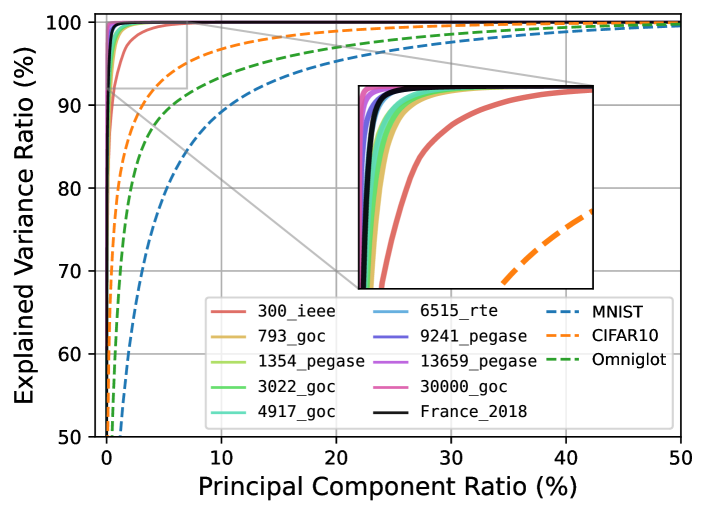
Figure 1: Explained Variance Ratios of PCA For the Various Principal Component Ratios for AC-OPF Instances (solid lines) and Natural Image Data (dashed lines).

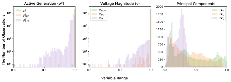
Figure 2: Histograms of Active Generations (left), Voltage Magnitudes (middle), and Principal Components (right) of the 20,000 Optimal Solutions in 1354_pegase. Three largest components on average are illustrated. The x-axis is normalized to $[0,1]$ using the minimum and maximum values.

(Almost) Lossless Compression

A key observation of the analysis is that PCA achieves an almost lossless compression with a few principal components. This is highlighted in Figure 1 where the x-axis represents the principal component ratio (i.e., the ratio of the number of the principal components in use to the dimension of the optimal solution) and the y-axis represents the explained variance ratio (i.e., the ratio of the cumulative sum of eigenvalues of the principal components in descending order to the sum of the all eigenvalues). The explained variance ratio is a proxy for how much the information is preserved within the chosen low-rank representation. For instance, the figure shows that $1\%$ of principal components preserves the $99.92\%$ of information of the AC-OPF optimal solutions for 13659_pegase. The detailed values are shown in Table II, which highlights that the compression is almost lossless with a 10% principal component ratio. This contrasts with data instances in computer vision, as exemplified by the MNIST [36], CIFAR10 [37], and Omniglot [38] datasets. This result is encouraging: it suggests that optimal solutions could be recovered with negligible losses when learning takes place in a low-rank space of a few principal components, potentially reducing the size of the mapping function substantially.

Larger Test Cases Need Fewer Principal Components

Figure 1 and Table II also highlight a desirable trend: larger test cases need a lower ratio of principal components to obtain the same level of explained variance ratio. For instance, the explained variance ratios of 13659_pegase and 30000_goc with a principal component ratio of $1\%$ are $99.92\%$ and $99.99\%$ respectively. In contrast, 300_ieee, the smallest test case, has $93.92\%$ of explained variance ratio. This observation shows that reducing the dimensionality through PCA is more effective for the bigger test cases and will be used in deciding the learning architecture for different test cases.

	Principal Component Ratio
Test case	1%	5%	10%	20%
300_ieee	93.92	99.56	99.97	99.99
793_goc	98.05	99.98	100.00	100.00
1354_pegase	99.04	99.98	100.00	100.00
3022_goc	98.64	99.99	100.00	100.00
4917_goc	99.03	99.99	100.00	100.00
6515_rte	99.74	99.99	100.00	100.00
9241_pegase	99.76	100.00	100.00	100.00
13659_pegase	99.92	100.00	100.00	100.00
30000_goc	99.99	100.00	100.00	100.00
France_2018	99.75	99.99	100.00	100.00
MNIST	44.45	79.12	89.17	95.27
CIFAR10	62.09	82.34	88.37	93.29
Omniglot	16.55	44.26	59.06	73.31

TABLE II: Explained Variance Ratios (%) on Various Principal Component Ratios from 1% to 20%.

Smoother Distributions on the Principal Components

Figure 2 provides some intuition for why learning in the space of the principal components is appealing. The figure shows the distributions of three active powers (left) and voltage magnitudes (middle) in the optimal solutions for the 1354_pegase test case. The values are plotted in log-scaled, highlighting the skewed nature of the active powers and voltage magnitudes: indeed, most values lie on their extreme limits. This has been observed before, leading to the use of the classification-then-regression approach [11]. However, fortunately, Figure 2 (right) shows that the distribution on the principal components is well-posed: it is more convenient to learn the regression to the low-rank space with a few principal components rather than to the original optimal solution space directly. As a result, the regression learning in the space of principal components should be easier than in the original space.

V Compact Optimization Learning

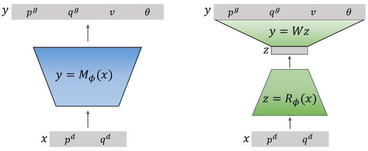
Figure 3: Schematic View of the Plain Approach (left) and Compact Learning (right).

The findings in Section IV suggest a Compact Learning model whose outputs are in the subspace defined by the principal components. This enables to decrease the number of trainable parameters in the DNN-based mapping function, reducing the memory footprint significantly.

V-A Compact Learning

The idea underlying Compact Learning is to jointly learn the principal components and the mapping between the original inputs and the outputs in the subspace of the principal components. Figure 3 contrasts the overall architecture of the Compact Learning with the conventional plain learning approach. The plain approach learns a mapping $y=M_{\phi}(x)$ from an input configuration $x$ to an optimal solution $y$, where $\phi$ are the associated trainable parameters. Since $y$ is high-dimensional, it is desirable to have a large number of parameters to obtain accurate solution estimates. Compact Learning in contrast learns a mapping $z=R_{\phi}(x)$ from an input configuration $x$ into an output $z$ in the subspace of principal components before recovering an optimal solution prediction as $y=Wz$. The output dimension of $R_{\phi}$, $\dim\left(z\right)$, in Compact Learning should be substantially smaller than the dimension of $y$, making it possible to reduce the number of trainable parameters. In the upcoming sections, the way of learning $R$ and $W$ simultaneously is detailed.

V-B Learning the Principal Components

Let $p$ and $d$ be the dimensions of $z$ and $y$, respectively, i.e., $p=\dim\left(z\right)$ and $d=\dim\left(y\right)$. The goal of Compact Learning is to have $p$ substantially smaller than $d$, i.e., $p\ll d$. Matrix $W\in\mathbb{R}^{d\times p}$ is unitary, i.e., $W^{\top}W=I$, and its columns are composed of the orthonormal principal components of the output space associated with $p$ largest eigenvalues. It is obviously possible to obtain $W$ through PCA, but this computation takes a substantial amount memory when there are many instances.

Instead, Compact Learning uses the Generalized Hebbian Algorithm (GHA), also called Sanger’s rule [39], to learn $W$ in a stochastic manner. GHA is specified in Algorithm 1. Using the mini-batch of optimal solutions $\{y^{*(i)}\}$, it first updates the element-wise running mean $\mu$ and variance $\sigma^{2}$ of optimal solution using the momentum parameter $\beta$. The momentum parameter $\beta$ is set to zero for the first iteration, and from the second iteration it is set to a value ranged $(0.0,1.0)$. The optimal solution $y^{*(i)}$ is normalized using the running mean and variance as shown in line 5 in Algorithm 1. GHA uses Gram-Schmidt process to find out the $\Delta W$ of the $p$ leading principal components, where $\mathcal{LT}[\cdot]$ represents the lower triangular matrix. Once $\Delta W$ is determined, $W$ is updated by adding $\gamma\Delta W$, where $\gamma$ is the learning rate that decreases as the epoch number $e$ increases, i.e.,

$$\gamma=\max\{\gamma_{\text{min}},\gamma_{\text{init}}/(0.01e)\},$$

In the update rule, $\gamma_{\text{init}}$ and $\gamma_{\text{min}}$ are hyperparameters representing the initial and minimum learning rate, respectively.

One can simply use deterministic PCA to define $W$ instead of using GHA. However this requires significant computing time before starting the training, especially when dealing with a large number of data instances of high dimensionality. In contrast, GHA amortizes the computational effort over the training procedure leading to a better handling of the largest test cases.

V-C Training the Compact Learning Model

Algorithm 1 Generalized Hebbian Algorithm,
GHA$(\{y^{(i)}\}_{i\in[B]},\!W,\!\mu,\!\sigma)$

Parameters:
   $\beta$: a momentum parameter
   $\gamma$: a learning rate for updating $W$
   $\epsilon$: a small positive for numerical stability

1:$m\leftarrow\frac{1}{B}\sum_{i=1}^{B}y^{(i)}$

2:$s^{2}\leftarrow\frac{1}{B}(y^{(i)}-m)^{2}$

3:$\mu\leftarrow\beta\mu+(1-\beta)m$ $\triangleright$ update running mean

4:$\sigma^{2}\leftarrow\beta\sigma^{2}+(1-\beta)s^{2}$ $\triangleright$ update running variance

5:$\hat{y}^{(i)}\leftarrow(y^{(i)}-\mu)/\sqrt{\sigma^{2}+\epsilon}$, $\;\forall i\in[B]$ $\triangleright$ normalize $y$

6:$\Delta W\!=\!\frac{1}{B}\!\sum_{i=1}^{B}\!\left(\hat{y}^{(i)}\hat{y}^{(i)\top}W\!-\!W\mathcal{LT}[W^{\top}\hat{y}^{(i)}\hat{y}^{(i)\top}W]\right)$

7:$W\leftarrow W+\gamma\Delta W$ $\triangleright$ update $W$

8:return $W$, $\mu$, $\sigma$.

Algorithm 2 Compact Learning

1:for $k$=1… do

2:     Sample $\{(x^{(i)},y^{*(i)}\}_{i\in[B]}$ from $\mathcal{D}$

3:     $W,\mu,\sigma\leftarrow$ GHA$(\{y^{*(i)}\}_{i\in[B]},W,\mu,\sigma)$

4:     $z^{(i)}=R_{\phi}(x^{(i)})$, $\;\forall i\in[B]$

5:     $y^{(i)}=\sqrt{\sigma^{2}\!+\!\epsilon}\,Wz^{(i)}\!+\!\mu$, $\;\forall i\in[B]$

6:     Update $\phi$ with $\mathcal{L}=\frac{1}{B}\sum_{i=1}^{B}\left\lVert{y^{(i)}}-{y^{*(i)}}\right\rVert_{1}$

7:end for

The training process of Compact Learning is summarized in Algorithm 2 which jointly learns the principal components $W$ and the mapping $R$. Each iteration samples a mini-batch of size $B$ and applies the GHA Algorithm 1 (line 3 in Algorithm 2). The mapping $R$ then produces $z^{(i)}$ for each input $x^{(i)}$ and the output $y^{(i)}$ is obtained through the mapping $Wz^{(i)}$ and a denormalization step (line 5 in Algorithm 2). Finally, the parameters $\phi$ associated with $R$ are updated using backpropagation from the loss function $\mathcal{L}$, which captures the mean absolute error between the prediction $y^{(i)}$ and the optimal solution $y^{*(i)}$ (ground truth).

V-D Restoring Feasibility

The predictions from Compact Learning may violate the physical and engineering constraints of the AC-OPF. Some applications are required to address these infeasibilities and this study considers two post-processing methods for this purpose: (1) solving the power flow problem; and (2) warm-starting the exact AC-OPF solver.

V-D1 Power Flow

The power flow problem, seeded with a prediction from the Compact Learning model, restores the feasibility of the physical constraints. Formally, the power flow problem can be formulated as:

find $$p^{g},q^{g},v,\theta,$$ (10)

subject to $$\text{Eq.~{}\eqref{eq:acopf_cnst_flow1}, \eqref{eq:acopf_cnst_flow2}},$$

$$\text{Eq.~{}\eqref{eq:acopf_cnst_balance}}.$$

In the power flow problem, like in [10], the active power injections and voltage magnitudes at the PV buses are fixed to the predictions. The power flow problem can then be solved by the Newton method to satisfy the physical constraints, i.e., Ohm’s law (Eq. (5a) and (5b)) and Kirchhoff’s Current Law (Eq. (6)). Finding a solution to the PF problem typically takes significantly less time than solving the AC-OPF. However, the solution may violate some of the engineering constraints of the AC-OPF.

V-D2 Warm-Starting the AC-OPF solver

It is possible to remove all infeasibilities by warm-starting an AC-OPF solver with the Compact Learning predictions. This study uses the primal-dual interior point algorithm Ipopt as a solver, which is a standard tool for solving AC-OPF problems [32, 40]. Moreover, warm-starts for the primal-dual interior point algorithm seem to benefit significantly from dual initial points. Hence, the Compact Learning model was generalized to predict dual optimal values for all constraints in addition to the primal optimal solutions. Ipopt is then warm-started with both primal and dual predictions to obtain an optimal solution.

VI Computational Experiments

VI-A The Experiment Setting

The performance of Compact Learning is demonstrated using nine test cases from PGLIB v21.07 and the realistic version of the French power system (denoted as France_2018) as described in Table I. A total of 52,000 instances were generated. 50,000 instances are used for training and the remaining 2,000 instances are tested for reporting the performance results. For the PGLib cases, these instances were obtained by perturbing the load demands as Eq (9) in Section IV: For France_2018, 100,000 instances for training are generated by perturbing the instances in September. Specifically, the upper bounds of active generation of the wind and hydro renewable generators are perturbed by replacing with the samples from $\mathcal{N}(\overline{p}^{g}_{i},0.2(\overline{p}^{g}_{i}-\underline{p}^{g}_{i}))$. Also, the upper bounds of solar generators and load demands are perturbed by multiplying factor sampled from multivariate Gaussian $\mathcal{N}(\mathbf{1},\Sigma)$ where $\Sigma$ is based on the correlation coefficient of $0.8$. Those perturbed upper bound of active generation is ensured to be greater than or equal to the lower bound of it. Also, 2000 realistic test instances are extracted from the instances in October for reporting the performance. As such, for this test case, the distribution of test instances is not necessarily the same as that of the training instances. Note that accurate renewable forecasting would improve the quality of the training instances, but this experiment setting for France_2018 should provide realistic and difficult circumstances where the model may be deployed for real operations. The instances were solved using Pyomo [41] and Ipopt v3.12 [34] with the HSL ma27 linear solver.

The performance of Compact Learning is compared with the plain approach that directly outputs the optimal solution. As in [10], four fully-connected layers followed by ReLU activations are used for the mapping functions for both Compact Learning and plain learning approaches. For the plain approach, two distinct models are experimented; the first model, which is named Plain-Large, has $d$ hidden nodes for each fully-connected layer (where $d$ is the output dimension). The second baseline, which is named Plain-Small, has the $p$ hidden nodes for each layer (where $p$ is the number of principal components considered in Compact Learning). The Compact Learning model has the same number of weight parameters as Plain-Small, but the last layer of the Compact Learning model is learned through GHA. Indeed, Plain-Small has an encoder-decoder structure as the number of the hidden nodes is smaller than that of the output. The ratio of $p$ to $d$, which is also called principal component ratio, is set to $5\%$ for six smaller test cases (up to 6515_rte) and to $1\%$ for four bigger cases. Mini-batch of $64$ instances is used, and the maximum epoch is set to $1,000$. The models are trained using the Adam optimizer [42] with a learning rate of $1\mathrm{e}{\textrm{-}4}$, which is decreased at $900$ epochs by $0.1$. The overall implementation used PyTorch and the models were trained on a machine with a NVIDIA Tesla V100 GPU and Intel Xeon 2.7GHz. For GHA (Algorithm 1), the momentum parameter $\beta$ is set to $0.9999$ from the second iteration. The initial and minimum learning rate ($\gamma_{\text{init}}$ and $\gamma_{\text{min}}$) are set to $1\mathrm{e}{\textrm{-}4}$, and $1\mathrm{e}{\textrm{-}8}$, respectively. The parameter $\epsilon$ to prevent ill-conditioning is set to $1\mathrm{e}{\textrm{-}8}$.

VI-B Learning Performance

Table III reports the accuracy of the models for predicting optimal solutions. Five distinct models with randomly initialized trainable parameters per method were trained: the results report the average results and the standard deviations (in parenthesis). The table shows the averaged value of optimality gaps and maximum constraint violations on the 2,000 test instances. The optimality gap is calculated as $100\times|\frac{f(y)-f(y^{*})}{f(y^{*})}|$ where $f(y)$ is the objective function (1). It also reports the maximum constraint violations (in per unit), which is computed as

$$\max\{\max_{i}\{\max\{g_{i}(y),0.\},\max_{i}\{|h_{i}(y)|\}\},$$ (11)

where $g_{i}(y)$ and $h_{i}(y)$ are, respectively, the inequality and equality constraints enumerated in Model 1. The first two sets of columns represent the performance of the plain approaches. Note that, because of the high dimensionality of the output and the limited GPU memory, Plain-Large is only applicable to the four smaller test cases (up to 3022_goc): this is the limitation that motivated this study. When comparing the two plain models, Plain-Large performs better than Plain-Small as Plain-Small trades off the accuracy for scalability. Compact Learning almost always performs better than the two plain approaches. In particular, it produces predictions with significantly fewer violations (sometimes by an order of magnitude), while also delivering smaller optimality gaps on the larger test cases.

Table IV shows the number of trainable parameters of the Compact Learning model and the plain approaches. The architectures of Compact Learning and Plain-Small are exactly the same, except for the last layer: hence the number of trainable parameters of Compact Learning is smaller than those for Plain-Small by the dimension of $W$. Table IV clearly shows that Compact Learning has the smallest number of trainable parameters. Overall, Table III and Table IV indicate that Compact Learning provides an accurate and scalable approach to predict AC-OPF solutions.

	Plain-Small		Plain-Large		Compact Learning (proposed)
Test case	Opt. Gap(%)	Viol.	Opt. Gap(%)	Viol.	Opt. Gap(%)	Viol.
300_ieee	0.9886(0.0287)	3.7282(0.0758)	0.1804(0.0087)	0.9256(0.0117)	0.1859(0.0079)	0.5509(0.0025)
793_goc	0.0579(0.0067)	3.1791(0.0985)	0.0182(0.0013)	0.5825(0.0046)	0.0305(0.0046)	0.2768(0.0033)
1354_pegase	0.1494(0.0142)	6.6858(0.1248)	0.0711(0.0094)	3.0360(0.1221)	0.0942(0.0089)	0.5044(0.0081)
3022_goc	0.0745(0.0105)	3.2394(0.0846)	0.0588(0.0094)	1.5837(0.1432)	0.0485(0.0076)	0.3906(0.0185)
4917_goc	0.0852(0.0118)	2.6590(0.1006)	-	-	0.0527(0.0087)	0.5456(0.0276)
6515_rte	0.7232(0.0364)	5.8648(0.2185)	-	-	0.3065(0.0177)	0.7519(0.0290)
9241_pegase	0.1521(0.0138)	6.7379(0.1980)	-	-	0.1344(0.0097)	1.1791(0.0725)
13659_pegase	0.0910(0.0057)	4.8141(0.0685)	-	-	0.0745(0.0046)	1.2915(0.0497)
30000_goc	0.2296(0.0224)	4.7172(0.0678)	-	-	0.1091(0.0112)	0.0770(0.0188)
France_2018	1.4872(0.1352)	47.4012(3.4524)	-	-	1.2869(0.0845)	2.1041(0.2218)

TABLE III: Performance Results of Compact Learning (Proposed) and Conventional Plain Learning Approaches (Baselines). Std. dev. in parenthesis is evaluated across five independent runs. Viol.: the mean value of the maximum constraint violations (in per unit) on the test instances. The best optimality gap (Opt. Gap) and maximum violation values are in bold.

Test case	Plain-Small	Plain-Large	Compact
300	0.045	2.479	0.019
793	0.274	14.487	0.122
1354	0.818	46.041	0.321
3022	3.631	200.572	1.499
4917	9.795	-	4.074
6515	17.202	-	7.353
9241	6.796	-	2.268
13659	16.954	-	4.442
30000	60.610	-	16.067
France	51.612	-	30.510

TABLE IV: The Number of Trainable Parameters (in Millions) in the Models Trained by Compact Learning and Plain Approaches.

VI-C Post-processing: Power Flow

One model among five trained models was randomly chosen for testing post-processing approaches and the results were evaluated on the same 2,000 test instances. Table V reports the constraint violations after applying the power flow model seeded with the predictions from the Compact Learning and Plain-Small models. The table also reports the time to solve the power flow problem. The results show that Compact Learning produces power flow solutions with the smallest constraint violations, sometimes by an order of magnitude. The results of Compact Learning are particularly impressive because the majority of the constraints are satisfied after applying the power flow. Note also that the power flow is fast enough to be used during real-time operations, opening interesting avenues for the use of learning and optimization in practice.

VI-D Post-processing: Warm-start

Table VI and Figure 4 report the results for warm-starts. The proposed warm-starting approach, WS:Compact(P+D), is compared with the following warm-starting strategies:

• Flat Start: $p^{g}$, $q^{g}$, $v$ are started with their minimum values, and initial $\theta$ is set to zero. This is a default setting without warm-start.

• WS:DC-OPF(P): Motivated from [20], the primal solution of the DC-OPF is used as a warm-starting point for solving AC-OPF.

• WS:AC-OPF(P): The primal solution of the AC-OPF is used as a warm-starting point for solving AC-OPF again.

• WS:Plain-Small(Large)(P): The primal predictions from the plain approaches are used as warm-starting points.

• WS:Plain-Small(Large)(P+D): The primal and dual predictions from the plain approaches are used as warm-starting points.

• WS:Compact(P): The primal predictions from Compact Learning are used as warm-starting points.

• WS:Compact(P+D): The proposed warm-starting approach. The primal and dual predictions from Compact Learning are used as warm-starting points.

	Plain-Small					Compact Learning
	Eq.(3a-4)		Eq. (7)		Time	Eq.(3a-4)		Eq. (7)		Time
Test case	Viol.(p.u.)	Sat(%)	Viol.(MVA)	Sat(%)	sec.	Viol.(p.u.)	Sat(%)	Viol.(MVA)	Sat(%)	sec.
4917_goc	0.1148	99.77	13.5821	99.47	1.07	0.0739	99.88	2.3134	99.50	1.15
6515_rte	0.2220	99.80	6.0533	99.92	1.54	0.0841	99.92	1.5261	99.95	1.58
9241_pegase	0.1338	99.47	10.3893	99.98	3.63	0.0893	99.82	2.4869	99.97	3.58
13659_pegase	0.2192	99.85	14.5279	99.99	7.11	0.0852	99.97	3.1203	100.00	7.01
30000_goc	0.0249	99.97	4.5279	100.00	10.27	0.0192	100.00	1.1958	100.00	10.11
France_2018	0.4073	99.98	11.5033	99.02	1.86	0.3788	99.98	3.2053	99.08	1.93

TABLE V: Averaged Maximum Violations and Ratio of Satisfied constraints (%) after Applying the Power Flow to AC-OPF Problems with $>$4,000 Buses.

	Primal	Dual	4917	6515	9241	13659	30000	France
Flat Start			8.90s	69.90s	44.67s	42.79s	163.48s	26.78s
WS:AC-OPF(P)	✓	✗	6.64s(1.34×)	10.10s(7.06×)	20.27s(2.22×)	28.45s(1.53×)	116.33s(1.43×)	9.66s(2.62×)
WS:DC-OPF(P)			10.68s(0.83×)	75.55s(0.90×)	53.59s(0.83×)	51.35s(0.83×)	196.17s(0.83×)	30.11s(0.85×)
WS:Plain-Small(P)			6.69s(1.33×)	10.06s(7.09×)	20.24s(2.22×)	28.24s(1.54×)	116.23s(1.43×)	10.04s(2.54×)
WS:Compact(P)			6.63s(1.34×)	10.05s(7.10×)	20.38s(2.21×)	28.41s(1.53×)	116.65s(1.43×)	9.83s(2.61×)
WS:Plain-Small(P+D)	✓	✓	3.16s(2.89×)	5.12s(14.79×)	17.31s(3.17×)	14.31s(3.05×)	16.54s(10.98×)	7.98s(3.65×)
WS:Compact(P+D)			2.49s(3.62×)	4.86s(15.26×)	15.59s(3.58×)	10.32s(4.23×)	15.66s(11.43×)	5.90s(4.84×)

TABLE VI: Averaged Elapsed Times (s) to Solve the AC-OPF Problems with $>$4,000 Buses and Averaged Speed-up Factor to Flat Start. The Best Values are in Bold.

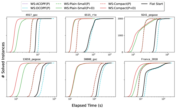
Figure 4: The Number of AC-OPF Instances Solved Within Various Elapsed Time Limits by Warm-Start (WS) and Flat Start.

Obviously, WS:DC-OPF(P) and WS:AC-OPF(P) need to solve the first problem to obtain the warm-starting points. For those, the time taken to solve the first problem is excluded in the reported elapsed time performance. Note that WS:AC-OPF(P) gives a virtual upper bound of the speed-up for primal-only warm-start for the primal-dual interior point algorithm. Also note that except for DC-OPF, the experiment does not include other convex relaxations of AC-OPF (e.g., the quadratic convex relaxation [43] and the semidefinite programming relaxations [44]), since solving those relaxed problems takes significant time.

To predict dual solutions, an additional mapping function consisting of four fully-connected layers is trained for Compact Learning and the plain approaches. The sizes of these networks are the same as those for the primal solutions. When using both the primal and dual warm-starting, the initial barrier parameter of Ipopt is set to $1\mathrm{e}{\textrm{-}6}$ because the initial warm-starting point is closer to the optimal than the flat start. The convergence tolerance is set to $1\mathrm{e}{\textrm{-}4}$ for all cases.

Table VI reports the elapsed times and the corresponding speed-up ratio for the warm-start approaches. The first key observation is that it is critical to use both primal and dual warm-starts: only using the primal predictions is not effective in reducing the computation times of Ipopt. This is not too surprising given the implementation of interior-point methods. Primal-dual warm-starts however produce significant benefits. WS:Compact(P+D) produces the best results for all test cases. In particular, it yields a speed-up of $15.26$× for 6515_rte. Also, even for the realistic French system (France_2018), WS:Compact(P+D) gives a speed-up of $4.84$×. This is significant given the realism of this test case and highlights the potential of the combination of Compact Learning and optimization to deploy AC-OPF in real operations. Observe also that WS:Compact(P+D) strongly dominates the other approaches, including its (WS:Plain-Small(P+D) counterpart. This was anticipated by its prediction errors reported earlier. Figure 4 depicts these results visually: it plots the number of AC-OPF instances solved over time by the various warm-starting methods. The plot clearly demonstrates the benefits of Compact Learning for predicting both primal and dual solutions.

VII Conclusions

This paper has proposed Compact Learning, a novel approach to predict optimal solutions to industry size OPF problems. Compact Learning was motivated by the lack of scalability of existing ML methods for this task. This difficulty stems from the dimension of the output space, which is large-scale in industry size AC-OPF problems. To address this issue, Compact Learning applies the PCA on the output space and learns in the subspace of a few leading principal components. It then combines this learning step with the GHA to learn the principal components, which is then used to transform the predictions back into the output space. Experimental results on industry size OPF problems show that Compact Learning is more accurate than existing approaches both in terms of optimality gaps and constraint violations, sometimes by an order of magnitude.

The paper also shows that the predictions can be used to accelerate the AC-OPF. In particular, the results show that the power flow problems seeded by the Compact Learning predictions have significantly fewer violations of the engineering constraints (while satisfying the physical constraints) for systems with up to 30,000 buses. Moreover, and even more interestingly, Compact Learning can be used to warm-start an OPF solver with optimal predictions for both the primal and dual variables. The results show that Compact Learning can produce significant speed-ups.

Together these results indicate that Compact Learning is the first method to produce high-quality predictions for the industry size OPFs that translate to significant practical benefits. There are also many opportunities for future research. Compact Learning is general-purpose and can be applied to other problems with large output space, which is typically the case in optimization. Nonlinear compression through autoencoder structure can be also considered for general-purpose optimization learning. On OPF problems, the performance of Compact Learning can be improved by adopting concepts from Lagrangian Duality, physics-informed networks, and different types of backbone architectures. The dual solution learning is particularly challenging in the experiments given its high dimensionality, and it would be interesting to study how it could be improved and simplified. Also, Compact Learning can be extended to learning solutions to more challenging problems such as Optimal Transmission Switching and Security-Constrained OPF in power system applications.

References

- [1] F. Safdarian, J. Snodgrass, J. H. Yeo, A. Birchfield, C. Coffrin, C. Demarco, S. Elbert, B. Eldridge, T. Elgindy, S. L. Greene et al., “Grid optimization competition on synthetic and industrial power systems,” 2022.
- [2] A. S. Zamzam and K. Baker, “Learning optimal solutions for extremely fast AC optimal power flow,” in 2020 IEEE International Conference on Communications, Control, and Computing Technologies for Smart Grids (SmartGridComm). IEEE, 2020, pp. 1–6.
- [3] F. Fioretto, T. W. Mak, and P. Van Hentenryck, “Predicting AC optimal power flows: Combining deep learning and Lagrangian dual methods,” in Proceedings of the AAAI Conference on Artificial Intelligence, vol. 34, no. 01, 2020, pp. 630–637.
- [4] B. Donon, Z. Liu, W. Liu, I. Guyon, A. Marot, and M. Schoenauer, “Deep statistical solvers,” Advances in Neural Information Processing Systems, vol. 33, pp. 7910–7921, 2020.
- [5] F. Diehl, “Warm-starting AC optimal power flow with graph neural networks,” in 33rd Conference on Neural Information Processing Systems (NeurIPS 2019), 2019, pp. 1–6.
- [6] D. Owerko, F. Gama, and A. Ribeiro, “Optimal power flow using graph neural networks,” in ICASSP 2020-2020 IEEE International Conference on Acoustics, Speech and Signal Processing (ICASSP). IEEE, 2020.
- [7] R. Nellikkath and S. Chatzivasileiadis, “Physics-informed neural networks for AC optimal power flow,” Electric Power Systems Research, vol. 212, p. 108412, 2022.
- [8] P. L. Donti, D. Rolnick, and J. Z. Kolter, “DC3: A learning method for optimization with hard constraints,” arXiv preprint arXiv:2104.12225, 2021.
- [9] S. Park and P. Van Hentenryck, “Self-supervised primal-dual learning for constrained optimization,” arXiv preprint arXiv:2208.09046, 2022.
- [10] M. Chatzos, T. W. Mak, and P. Van Hentenryck, “Spatial network decomposition for fast and scalable AC-OPF learning,” IEEE Transactions on Power Systems, vol. 37, no. 4, pp. 2601–2612, 2021.
- [11] W. Chen, S. Park, M. Tanneau, and P. Van Hentenryck, “Learning optimization proxies for large-scale security-constrained economic dispatch,” Electric Power Systems Research, vol. 213, p. 108566, 2022.
- [12] Á. S. Xavier, F. Qiu, and S. Ahmed, “Learning to solve large-scale security-constrained unit commitment problems,” INFORMS Journal on Computing, vol. 33, no. 2, pp. 739–756, 2021.
- [13] A. V. Ramesh and X. Li, “Feasibility layer aided machine learning approach for day-ahead operations,” arXiv preprint arXiv:2208.06742, 2022.
- [14] S. Park, W. Chen, D. Han, M. Tanneau, and P. Van Hentenryck, “Confidence-aware graph neural networks for learning reliability assessment commitments,” arXiv preprint arXiv:2211.15755, 2022.
- [15] M. Chatzos, F. Fioretto, T. W. Mak, and P. Van Hentenryck, “High-fidelity machine learning approximations of large-scale optimal power flow,” arXiv preprint arXiv:2006.16356, 2020.
- [16] T. W. Mak, M. Chatzos, M. Tanneau, and P. Van Hentenryck, “Learning regionally decentralized AC optimal power flows with ADMM,” arXiv preprint arXiv:2205.03787, 2022.
- [17] D. Deka and S. Misra, “Learning for DC-OPF: Classifying active sets using neural nets,” in 2019 IEEE Milan PowerTech. IEEE, 2019, pp. 1–6.
- [18] F. Cengil, H. Nagarajan, R. Bent, S. Eksioglu, and B. Eksioglu, “Learning to accelerate globally optimal solutions to the AC optimal power flow problem,” Electric Power Systems Research, vol. 212, p. 108275, 2022.
- [19] K. Sundar, H. Nagarajan, S. Misra, M. Lu, C. Coffrin, and R. Bent, “Optimization-based bound tightening using a strengthened QC-relaxation of the optimal power flow problem,” arXiv preprint arXiv:1809.04565, 2018.
- [20] A. Venzke, S. Chatzivasileiadis, and D. K. Molzahn, “Inexact convex relaxations for AC optimal power flow: Towards AC feasibility,” Electric Power Systems Research, vol. 187, p. 106480, 2020.
- [21] B. Taheri and D. K. Molzahn, “Restoring AC power flow feasibility from relaxed and approximated optimal power flow models,” arXiv preprint arXiv:2209.04399, 2022.
- [22] K. Baker, “Learning warm-start points for AC optimal power flow,” in 2019 IEEE 29th International Workshop on Machine Learning for Signal Processing (MLSP). IEEE, 2019, pp. 1–6.
- [23] W. Dong, Z. Xie, G. Kestor, and D. Li, “Smart-PGSim: Using neural network to accelerate AC-OPF power grid simulation,” in SC20: International Conference for High Performance Computing, Networking, Storage and Analysis. IEEE, 2020, pp. 1–15.
- [24] X. Pan, M. Chen, T. Zhao, and S. H. Low, “DeepOPF: A feasibility-optimized deep neural network approach for AC optimal power flow problems,” IEEE Systems Journal, 2022.
- [25] X. Lei, Z. Yang, J. Yu, J. Zhao, Q. Gao, and H. Yu, “Data-driven optimal power flow: A physics-informed machine learning approach,” IEEE Transactions on Power Systems, vol. 36, no. 1, pp. 346–354, 2020.
- [26] J. Liu, Z. Yang, J. Zhao, J. Yu, B. Tan, and W. Li, “Explicit data-driven small-signal stability constrained optimal power flow,” IEEE Transactions on Power Systems, vol. 37, no. 5, pp. 3726–3737, 2021.
- [27] J. B. Ward, “Equivalent circuits for power-flow studies,” Transactions of the American Institute of Electrical Engineers, vol. 68, no. 1, pp. 373–382, July 1949.
- [28] W. Jang, S. Mohapatra, T. J. Overbye, and H. Zhu, “Line limit preserving power system equivalent,” in 2013 IEEE Power and Energy Conference at Illinois (PECI), 2013, pp. 206–212.
- [29] S. Y. Caliskan and P. Tabuada, “Kron reduction of power networks with lossy and dynamic transmission lines,” in 2012 IEEE 51st IEEE Conference on Decision and Control (CDC), 2012, pp. 5554–5559.
- [30] I. P. Nikolakakos, H. H. Zeineldin, M. S. El-Moursi, and J. L. Kirtley, “Reduced-order model for inter-inverter oscillations in islanded droop-controlled microgrids,” IEEE Transactions on Smart Grid, vol. 9, no. 5, pp. 4953–4963, 2018.
- [31] Z. Jiang, N. Tong, Y. Liu, Y. Xue, and A. G. Tarditi, “Enhanced dynamic equivalent identification method of large-scale power systems using multiple events,” Electric Power Systems Research, vol. 189, p. 106569, 2020.
- [32] S. Babaeinejadsarookolaee, A. Birchfield, R. D. Christie, C. Coffrin, C. DeMarco, R. Diao, M. Ferris, S. Fliscounakis, S. Greene, R. Huang et al., “The power grid library for benchmarking AC optimal power flow algorithms,” arXiv preprint arXiv:1908.02788, 2019.
- [33] M. Chatzos, M. Tanneau, and P. Van Hentenryck, “Data-driven time series reconstruction for modern power systems research,” Electric Power Systems Research, vol. 212, p. 108589, 2022.
- [34] A. Wächter and L. T. Biegler, “On the implementation of an interior-point filter line-search algorithm for large-scale nonlinear programming,” Mathematical programming, vol. 106, no. 1, pp. 25–57, 2006.
- [35] “eco2mix,” https://www.rte-france.com/en/eco2mix.
- [36] Y. LeCun and C. Cortes, “MNIST handwritten digit database,” 2010. [Online]. Available: http://yann.lecun.com/exdb/mnist/
- [37] A. Krizhevsky, G. Hinton et al., “Learning multiple layers of features from tiny images,” 2009.
- [38] B. M. Lake, R. Salakhutdinov, and J. B. Tenenbaum, “Human-level concept learning through probabilistic program induction,” Science, vol. 350, no. 6266, pp. 1332–1338, 2015.
- [39] T. D. Sanger, “Optimal unsupervised learning in a single-layer linear feedforward neural network,” Neural networks, vol. 2, no. 6, pp. 459–473, 1989.
- [40] S. Gopinath and H. L. Hijazi, “Benchmarking large-scale ACOPF solutions and optimality bounds,” arXiv preprint arXiv:2203.11328, 2022.
- [41] W. E. Hart, C. D. Laird, J.-P. Watson, D. L. Woodruff, G. A. Hackebeil, B. L. Nicholson, J. D. Siirola et al., Pyomo-optimization modeling in python. Springer, 2017, vol. 67.
- [42] D. P. Kingma and J. Ba, “Adam: A method for stochastic optimization,” arXiv preprint arXiv:1412.6980, 2014.
- [43] C. Coffrin, H. L. Hijazi, and P. Van Hentenryck, “The QC relaxation: A theoretical and computational study on optimal power flow,” IEEE Transactions on Power Systems, vol. 31, no. 4, pp. 3008–3018, 2015.
- [44] X. Bai, H. Wei, K. Fujisawa, and Y. Wang, “Semidefinite programming for optimal power flow problems,” International Journal of Electrical Power & Energy Systems, vol. 30, no. 6-7, pp. 383–392, 2008.