Active Learning of
Piecewise Gaussian Process Surrogates

Abstract

Active learning of Gaussian process (GP) surrogates has been useful for optimizing experimental designs for physical/computer simulation experiments, and for steering data acquisition schemes in machine learning. In this paper, we develop a method for active learning of piecewise, Jump GP surrogates. Jump GPs are continuous within, but discontinuous across, regions of a design space, as required for applications spanning autonomous materials design, configuration of smart factory systems, and many others. Although our active learning heuristics are appropriated from strategies originally designed for ordinary GPs, we demonstrate that additionally accounting for model bias, as opposed to the usual model uncertainty, is essential in the Jump GP context. Toward that end, we develop an estimator for bias and variance of Jump GP models. Illustrations, and evidence of the advantage of our proposed methods, are provided on a suite of synthetic benchmarks, and real-simulation experiments of varying complexity.

Keywords: Piecewise Regression, Divide-and-Conquer, Bias–Variance Tradeoff, Sequential Design, Active Learning

1 Introduction

The main goal of machine learning is to create an autonomous computer system that can learn from data with minimal human intervention (Mitchell, 1997). In many machine learning tasks, one can control the data acquisition process in order to select training examples that target specific goals. Active learning (AL) – or sequential design of experiments in classical statistical jargon – is the study of how to select data toward optimizing a given learning objective (e.g., Cohn et al., 1996; Lam & Notz, 2008). Here we consider AL for piecewise continuous Gaussian process (GP) regression models.

Our motivating application is surrogate modeling (Gramacy, 2020) of modern engineering systems, to explore and understand overall system performance and ultimately to optimize aspects of their design. A particular focus here is on engineering systems whose behaviors intermittently exhibit abrupt jumps or local discontinuities across regimes of a design space. Such “jump system” behaviors are found in many applications. For example, carbon nanotube yield from a chemical vapor deposition (CVD) process (Magrez et al., 2010) varies depending on many design variables. Changes in dynamics are mostly gradual, but process yield can suddenly jump around, depending on chemical equilibrium conditions, from ‘no-growth’ to ‘growth’ regions (Nikolaev et al., 2016). Illustration is provided in the right panel of Figure 1. Specific boundary conditions dictating these regime shifts depend on experimental and system design details. Such jump system behaviors are universal to many material and chemistry applications owing to several factors (i.e., equilibrium, phase changes, activation energy). Jump behaviors are also frequently seen in engineering systems operating near capacity. When a system runs below its capacity, performance is generally good and exhibits little fluctuation. However, performance can suddenly break down as the system is forced to run slightly over its capacity (Kang et al., 2022).

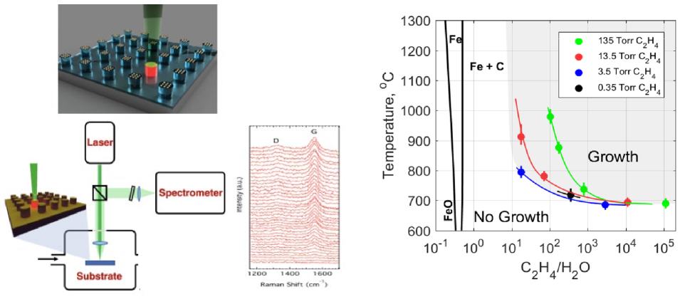
Figure 1: Process yield prediction for carbon nanotube synthesis. Left: a chemical vapor deposition (CVD) process integrated with in-line Raman spectrometer measurements of nanotube yields. Right: response surface(s) of carbon nanotube yields as a function of reaction temperature and a ratio of two chemical ingredients.

Suitable surrogate models for jump systems must accommodate piecewise continuous functional relationships, where disparate input–output dynamics can be learned (if data from the process exemplify them) in geographically distinct regions on input/configuration space. Most existing surrogate modeling schemes make an assumption of stationarity, and are thus not well-suited to such processes. AL strategies paired with such surrogates are, consequently, sub-optimal for acquiring training examples in such settings. For example, Gaussian processes (GPs; Rasmussen & Williams, 2006) are perhaps the canonical choice for surrogate modeling of physical and computer experiments (Santner et al., 2018). They are flexible, nonparametric, nonlinear, lend a degree of analytic tractability, and provide well-calibrated uncertainty quantification without having to tune many unknown quantities. But the canonical, relative-distance-based kernels used with GPs result in stationary processes. Therefore, AL schemes paired with GPs exhibit un-interesting, space-filling behavior. Representative examples includes “Active Learning Cohn” (Cohn et al., 1996, ALC), “Active Learning-MacKay” (McKay et al., 2000, ALM), and “Active Learning with Mutual Information” (Krause et al., 2008; Beck & Guillas, 2016, MI). Space-filling designs, and their sequential analogues, are inefficient when input–output dynamics change across regions of the input space. Intuitively, we need a higher density of training examples in harder-to-model regions, and near boundaries where regime dynamics change.

Regime-changing dynamics are inherently non-stationary: both position and relative distance information (in the input configuration space) is required for effective modeling. Examples of non-stationary GP modeling strategies from the geospatial literature abound (Sampson & Guttorp, 1992; Schmidt & O’Hagan, 2003; Paciorek & Schervish, 2006). The trouble with these approaches is that they are too slow, in many cases demanding enormous computational resources in their own right, or limited to two input dimensions. Recent developments in the machine learning literature around deep GPs (Damianou & Lawrence, 2013) represent a promising alternative. Input dimensions can be larger, and fast inference is provided by doubly stochastic variational inference (Salimbeni & Deisenroth, 2017). But such methods are data-hungry, requiring tens of thousands of training examples before they are competitive with conventional GP methods. We will illustrate this later with a small toy example in Section 5.1. An ALC-type active learning criterion has been developed for deep GPs (Sauer et al., 2020), making them less data-hungry but computational expense for Markov chain Monte Carlo (MCMC) inference is still a bottleneck.

A class of methods built around divide-and-conquer strategies can offer the best of both worlds – computational thrift with modeling fidelity – by simultaneously imposing statistical and computational independence. The best-known examples include treed GPs (Gramacy & Lee, 2008; Taddy et al., 2011; Malloy & Nowak, 2014; Konomi et al., 2014) and Voronoi tessellation-based GPs (Kim et al., 2005; Heaton et al., 2017; Pope et al., 2021; Luo et al., 2021). Partitioning facilitates non-stationrity almost trivially, by independently fitting different GPs in different parts of the input space. But learning the partition can be challenging. Sequential design/AL criteria have been adapted to some of these divide-and-conquer surrogates. ALM and ALC, for example, have been adapted for treed GPs (Gramacy & Lee, 2009; Taddy et al., 2011). However the axis-aligned nature of the treed GP is not flexible enough to handle the complex, nonlinear manifold of regime change exhibited of many real datasets, as illustrated empirically in Section 5.1.

Park (2022) introduced the Jump GP to address this limitation. This approach seeks a local approximation to an otherwise potentially complex domain-partitioning and GP-modeling scheme. Crucially, direct inference for the Jump GP enjoys the same degree of analytic tractability as an ordinary, stationary GP. However, good AL strategies have not been studied for the Jump GP model, which is the main focus of this paper. We are inspired by related work in jump kernel regression (Park et al., 2023). However, it is important to remark that that work focused on more limited class of (non-GP) nonparametric regression models. In the context of the Jump GP for nonstationary surrogate modeling, we propose to extend conventional AL strategies to consider model bias in addition to the canonical variance-based heuristics. We show that considering bias is essential in a non-stationary modeling setting. In particular, ordinary stationary GP surrogates can exhibit substantial bias for test location nearby regime changes. The Jump GP can help mitigate this bias, but it does not completely remove it. Consequently established AL strategies that don’t incorporate estimates of bias are limited in their ability to improve sequential learning of the Jump GP. The major contribution of this paper is to estimate both bias and variance for Jump GPs and parlay these into novel AL strategies for nonstationary surrogate modeling.

The remainder of the paper is outlined as follows. In Section 2, we review relevant topics around Jump GP and AL with an eye toward motivating our novel contribution. Section 3 develops joint bias and variance estimation for Jump GPs. Using those estimates, we develop three AL heuristics for Jump GPs in Section 4. We illustrate the numerical performance of the proposed heuristics using a synthetic benchmark and two real data/simulation cases in Section 5. A summary and brief discussion concludes the paper Section 6.

2 Review

Here we review components essential to framing our contribution: GP surrogates, AL, partition-based modeling and the Jump GP.

2.1 Stationary GP surrogates

Let $\mathcal{X}$ denote a $d$-dimensional input configuration space. Consider a problem of estimating an unknown function $f:\mathcal{X}\rightarrow\mathbb{R}$ relating inputs $\boldsymbol{x}_{i}\in\mathcal{X}$ to a noisy real-valued response variable $y_{i}\stackrel{{\scriptstyle\mathrm{iid}}}{{\sim}}\mathcal{N}(f(\boldsymbol{x}_{i}),\sigma^{2})$ though examples composed as training data, $\mathcal{D}_{N}=\{(\boldsymbol{x}_{i},y_{i}),\;i=1,\ldots,N\}$. In GP regression, a finite collection $\boldsymbol{f}_{N}=(f_{1},\dots,f_{N})$ of $f(\boldsymbol{x}_{i})\equiv f_{i}$ values is modeled as a multivariate normal (MVN) random variable. A common specification involves a constant, scalar mean $\mu$, and $N\times N$ correlation matrix $C_{N}$: $\boldsymbol{f}_{N}\sim\mathcal{N}_{N}(\mu\mathbf{1}_{N},\boldsymbol{C}_{N})$.

Rather than treating all $\mathcal{O}(N^{2})$ values in $\boldsymbol{C}_{N}$ as “tunable parameters”, it is common to use a kernel $c(\boldsymbol{x}_{i},\boldsymbol{x}_{j};\theta)$ defining correlations in terms of a small number of hyperparameters $\theta$. Most kernel families (Abrahamsen, 1997; Wendland, 2004) are decreasing functions of the geographic “distance” between it’s arguments $\boldsymbol{x}_{i}$ and $\boldsymbol{x}_{j}$. Our contributions are largely agnostic to these choices. An assumption of stationarity is common, whereby $c(\boldsymbol{x}_{i},\boldsymbol{x}_{j};\theta)\equiv c(\boldsymbol{x}_{i}-\boldsymbol{x}_{j};\theta)$, i.e., only relative displacement $\boldsymbol{x}_{i}-\boldsymbol{x}_{j}$ between inputs, not their positions, matters for modeling. As discussed further, below, a stationarity assumption can be limiting and relaxing this is a major focus of the methodology introduced in this paper.

Integrating out latent $\boldsymbol{f}_{N}$ values, to obtain a distribution for $\boldsymbol{y}_{N}$, is straightforward because both are Gaussian. This leads to the marginal likelihood $\boldsymbol{y}_{N}\sim\mathcal{N}_{N}(\mu\mathbf{1}_{N},\boldsymbol{C}_{N}+\sigma^{2}\mathbb{I}_{N})$ which can be used to learn hyperparameters. Maximum likelihood estimates (MLEs), $\hat{\mu}$ and $\hat{\sigma}^{2}$, have closed forms conditional on $\theta$. E.g., Mu et al. (2017) provides $\hat{\mu}=\boldsymbol{1}_{N}^{T}(\hat{\sigma}^{2}\boldsymbol{I}_{N}+\boldsymbol{C}_{N})^{-1}\boldsymbol{y}_{N}/\boldsymbol{1}_{N}^{T}(\hat{\sigma}^{2}\boldsymbol{I}_{N}+\boldsymbol{C}_{N})^{-1}\boldsymbol{1}_{N}$. Estimates for $\hat{\theta}$ depend on the kernel and generally requires numerical methods. For details, see Rasmussen & Williams (2006); Santner et al. (2018); Gramacy (2020).

Analytic tractability extends to prediction. Basic MVN conditioning from a joint model of $\boldsymbol{Y}_{N}$ and an unknown testing output $Y(\boldsymbol{x}_{*})$ gives that $Y(\boldsymbol{x}_{*})\mid\boldsymbol{y}_{N}$ is univariate Gaussian. Below we quote the distribution for the latent function value $\hat{f}(\boldsymbol{x})\equiv f(\boldsymbol{x}_{*})\mid\boldsymbol{y}_{N}$, which is of more direct interest in our setting. This distribution is also Gaussian, with

$$\begin{array}[]{l l}\mbox{mean: }&\mu(\boldsymbol{x}_{*})=\hat{\mu}+\boldsymbol{c}_{N}^{T}(\sigma^{2}\boldsymbol{I}_{N}+\boldsymbol{C}_{N})^{-1}(\boldsymbol{y}_{N}-\hat{\mu}\boldsymbol{1}_{N}),\mbox{ and }\\ \mbox{variance: }&s^{2}(\boldsymbol{x}_{*})=c(\boldsymbol{x}_{*},\boldsymbol{x}_{*};\hat{\theta})-\boldsymbol{c}_{N}^{T}(\hat{\sigma}^{2}\mathbb{I}_{N}+\boldsymbol{C}_{N})^{-1}\boldsymbol{c}_{N},\end{array}$$ (1)

where $\boldsymbol{c}_{N}=[c(\boldsymbol{x}_{i},\boldsymbol{x}_{*};\hat{\theta}):i=1,...,N]$ is a $N\times 1$ vector of the covariance values between the training data and the test data point. Observe that evaluating these prediction equations, like evaluating the MVN likelihood for hyperparameter inference, requires inverting the $N\times N$ matrix $\boldsymbol{C}_{N}$. So although there is a high degree of analytic tractability, there are still substantial numerical hurdles to application in large-data settings.

2.2 Divide-and-conquer GP modeling

Partitioned GP models (Gramacy & Lee, 2008; Kim et al., 2005), generally, and the Jump GP (Park, 2022), specifically, consider an $f$ that is piecewise continuous

$$f(\boldsymbol{x})=\sum_{k=1}^{K}f_{k}(\boldsymbol{x})1_{\mathcal{X}_{k}}(\boldsymbol{x}),$$ (2)

where $\mathcal{X}_{1},\mathcal{X}_{2},\ldots,\mathcal{X}_{K}$ are a partition of $\mathcal{X}$. Above, $1_{\mathcal{X}_{k}}(\boldsymbol{x})$ is an indicator function that determines whether $\boldsymbol{x}$ belongs to region $\mathcal{X}_{k}$, and each $f_{k}(\boldsymbol{x})$ is a continuous function that serves as a basis for the regression model on region $\mathcal{X}_{k}$. Although variations abound, here we take each functional piece $f_{k}(\boldsymbol{x})$ to be a stationary GP, as described in Section 2.1.

Typically, each $f_{k}$ is taken to independent conditional on the partitioning mechanism. This assumption is summarized below for easy referencing later.

$$\mbox{Independence:}\qquad f_{k}\mbox{ is independent of }f_{j}\mbox{ for }j\neq k.$$ (3)

Consequently, all hyperparameters describing $f_{k}$ may be analogously indexed and are treated independently, e.g., $\mu_{k}$, $\sigma_{k}^{2}$ and $\theta_{k}$. Generally speaking, the data within region $\mathcal{X}_{k}$ are used to learn these hyperparameters, via the likelihood applied on the subset of data $\mathcal{D}_{N}$ whose $\boldsymbol{x}$-locations reside in $\mathcal{X}_{k}$. Although it is possible to allow novel kernels $c_{k}$ in each region, it is common to fix a particular form (i.e., a family) for use throughout. Only it’s hyperarmeters $\theta_{k}$ vary across regions, as in $c(\cdot,\cdot;\theta_{k}$). Predicting with $\hat{f}(\boldsymbol{x}_{*})$, conditional on a partition and estimated hyperparameters, is simply a matter of following Eq. (2) with “hats”. That is, with $\hat{f}_{k}$ defined analogously to Eq. (1), i.e., using only $y$-values exclusive to each region. In practice, the sum over indicators in Eq. (2) is bypassed and one simply identifies the $\mathcal{X}_{k}$ to which $\boldsymbol{x}_{*}$ belongs and uses the corresponding $\hat{f}_{k}$ directly.

Popular, data-driven partitioning schemes leveraging local stationary GP models include Voronoi tessellation (Kim et al., 2005; Heaton et al., 2017; Pope et al., 2021; Luo et al., 2021) or recursive axis-aligned, tree-based partitioning (Gramacy & Lee, 2008; Taddy et al., 2011; Malloy & Nowak, 2014; Konomi et al., 2014). These “structures”, defining $K$, and within-partition hyperparameters $(\mu_{k},\theta_{k},\sigma^{2})$ may be jointly learned, via posterior sampling (e.g., MCMC) or by maximizing marginal likelihoods. In so doing, one is organically learning a degree of non-stationarity. Independent GPs, via disparate independently learned hyperparameters, facilitate a position-dependent correlation structure. Learning separate $\sigma_{k}^{2}$ in each region can also accommodate heteroskedasticy (Binois et al., 2018). Such divide-and-conquer can additionally bring computational gains, through smaller-$N$ calculations within each region of the partition.

2.3 Local GP modeling

Although there are many example settings where such partition-based GP models excel, their rigid structure can be a mismatch to many important real-data settings. The Jump GP (JGP; Park, 2022) is motivated by such applications. The idea is best introduced through the lens of local, approximate GP modeling (LAGP; Gramacy & Apley, 2015). For each test location $\boldsymbol{x}_{*}$, select a small subset of training data nearby $\boldsymbol{x_{*}}$: $\mathcal{D}_{n}(\boldsymbol{x}_{*})=\{(\boldsymbol{x}_{i,*},y_{i,*})\}_{i=1}^{n}\subset\mathcal{D}_{N}$. Then, fit a conventional, stationary GP model $\hat{f}_{n}(\boldsymbol{x}_{*})$ to the local data $\mathcal{D}_{n}(\boldsymbol{x}_{*})$. This is fast, because $\mathcal{O}(n^{3})$ is much better than $\mathcal{O}(N^{3})$ when $n\ll N$, and massively parallelizable over many $\boldsymbol{x}_{*}\in\mathcal{X}$ (Gramacy et al., 2014). It is has a nice divide-and-conquer structure, but it is not a partition model (2). Nearby $\mathcal{D}_{n}(\boldsymbol{x}_{*}^{\prime})$ might have some, all, or no elements in common. LAGP can furnish biased predictions (Park, 2022) because independence (3) is violated: local data $\mathcal{D}_{n}(\boldsymbol{x}_{*}^{\prime})$ might mix training examples from regions of the input space exhibiting disparate input-output dynamics.

A JGP differs from basic LAGP modeling by selecting local data subsets in such a way as a partition (2) is maintained and independence (3) is enforced, so that bias is reduced. Toward this end, the JGP introduces an latent, binary random variable $Z_{i}\in\{0,1\}$ to express uncertainties on whether a local data point $\boldsymbol{x}_{i,*}$ belongs to a region of the input exhibiting the same (stationary) input-output dynamics as the test location $\boldsymbol{x}_{*}$, or not:

$$Z_{i}=\left\{\begin{array}[]{c l}1&\mbox{ if }\boldsymbol{x}_{i,*}\mbox{ and }\boldsymbol{x}_{*}\mbox{ belong to the same region}\\ 0&\mbox{ otherwise}.\end{array}\right.$$

Conditional on $Z_{i}$ values, $i=1,\dots,N$, we may partition the local data $\mathcal{D}_{n}$ into two groups: $\mathcal{D}_{*}=\{i=1,\ldots,n:Z_{i}=1\}$ and $\mathcal{D}_{o}=\{1,\ldots,n\}\backslash\mathcal{D}_{*}$, lying in regions of the input space containing $\boldsymbol{x}_{*}$ and not, respectively.

Complete the specification by modeling $\mathcal{D}_{*}$ with a stationary GP [Section 2.1], $\mathcal{D}_{o}$ with dummy likelihood $p(y_{i,*}\mid Z_{i}=0)\propto U$ for some constant, $U$, and assign a prior for the latent variable $Z_{i}$ via a sigmoid $\pi$ on an unknown partitioning function $g(\boldsymbol{x},\boldsymbol{\omega})$,

$$p(Z_{i}=1|\boldsymbol{x}_{i,*},\boldsymbol{\omega})=\pi(g(\boldsymbol{x}_{i,*},\boldsymbol{\omega})),$$ (4)

where $\boldsymbol{\omega}$ is another hyperparameter. Specifically, for $\boldsymbol{Z}=(Z_{i},i=1,\ldots,n)$, $\boldsymbol{f}_{*}=(f_{i,*},i=1,\ldots,n)$ and $\boldsymbol{\Theta}=\{\boldsymbol{\omega},m_{*},\theta_{*},\sigma^{2}\}$, the JGP model may be summarized as follows.

$$p(\boldsymbol{y}_{n}\mid\boldsymbol{f}_{*},\boldsymbol{Z},\boldsymbol{\Theta}) =\prod_{i=1}^{n}\mathcal{N}_{1}(y_{i,*}|f_{i,*},\sigma^{2})^{Z_{i}}U^{1-Z_{i}},$$

$$p(\boldsymbol{Z}\mid\boldsymbol{\omega}) =\prod_{i=1}^{n}\pi(g(\boldsymbol{x}_{i,*},\boldsymbol{\omega}))^{Z_{i}}(1-\pi(g(\boldsymbol{x}_{i,*},\boldsymbol{\omega})))^{1-Z_{i}},$$

$$p(\boldsymbol{f}_{*}\mid m_{*},\theta_{*}) =\mathcal{N}_{n}(\boldsymbol{f}_{*}\mid m_{*}\boldsymbol{1}_{n},\boldsymbol{C}_{nn}),$$

where $\boldsymbol{y}_{n}=(y_{i,*},i=1,\ldots,n)$ and $\boldsymbol{C}_{nn}=[c(\boldsymbol{x}_{i,*},\boldsymbol{x}_{i,*};\theta_{*}):i,j=1,...,n]$ is a square matrix of the covariance values evaluated for all pairs of the local data $\mathcal{D}_{n}(\boldsymbol{x}_{*})$.

Conditional on $\boldsymbol{\Theta}$, prediction $\hat{f}(\boldsymbol{x}_{*})$ follows the usual equations (1) using local data $\mathcal{D}_{n}(\boldsymbol{x}_{*})$. A detailed presentation is delayed, along with further discussion, until Section 3. Inference for latent $\boldsymbol{Z}$ may proceed by expectation maximization (EM; Dempster et al., 1977). However, a difficulty arises because the joint posterior distribution of $\boldsymbol{Z}$ and $\boldsymbol{f}_{*}$ is not tractable, complicating the E-step. As a workaround, Park (2022) developed a classification EM (CEM; Bryant & Williamson, 1978; Gupta & Chen, 2010) variation which replaces the E-step with a pointwise maximum a posteriori (MAP) of $\hat{\boldsymbol{Z}}$.

2.4 Active Learning for GPs

Active learning (AL) attempts to sustain a virtuous cycle between data collection and model learning. Begin with training data of size $N$, $\mathcal{D}_{N}=\{(\boldsymbol{x}_{i},y_{i}),i=1,\ldots,N\}$, such as a space-filling Latin hypercube design (LHD; Lin & Tang, 2015). Then augment $\mathcal{D}_{N}$ with a new data point $(\boldsymbol{x}_{N+1},y_{N+1})$ chosen to optimize a criterion quantifying an important aspect or capability of the model, and repeat. Perhaps the canonical choice is mean square prediction error (MSPE), comprising of squared bias and variance (Hastie et al., 2009).

Many machine learning algorithms are equipped with the proofs of unbiasedness of predictions under regularity conditions. When training and testing data jointly satisfy a stationarity assumption, the GP predictor (1) is unbiased, and so the MSPE is equal to $s^{2}(\boldsymbol{x}_{*})$. Consequently, many AL leverage this quantity. For example, the “Active Learning-MacKay” (ALM; McKay et al., 2000) maximizes it directly: $\boldsymbol{x}_{N+1}=\operatorname*{\arg\!\max}_{\boldsymbol{x}_{*}\in\mathcal{X}}\;s(\boldsymbol{x}_{*})$. In repeated application, this AL strategy can be shown to approximate a maximum entropy design (Gramacy, 2020, Section 6.3).

An integrated mean squared prediction error (IMSPE) criterian considers how the MSPE of GP is affected, globally in the input space, after injecting new data at $\boldsymbol{x}_{N+1}$. Let $s^{2}_{N+1}(\boldsymbol{x}_{*})$ denote the predictive variance (1) a test location $\boldsymbol{x}_{*}$, when the training data $\mathcal{D}_{N}$ is augmented with one additional input location $\boldsymbol{x}_{N+1}$:

$$s^{2}(\boldsymbol{x}_{*};\boldsymbol{x}_{N+1})=c(\boldsymbol{x}_{*},\boldsymbol{x}_{*};\hat{\theta})-\boldsymbol{c}_{N+1}^{T}(\hat{\sigma}^{2}\boldsymbol{I}_{N+1}+\boldsymbol{C}_{N+1})^{-1}\boldsymbol{c}_{N+1},$$

where $\boldsymbol{c}_{N+1}=[c(\boldsymbol{x}_{i},\boldsymbol{x}_{*};\hat{\theta}):i=1,...,N+1]$, $\boldsymbol{C}_{N+1}$ analogousy via $\hat{\theta}$ via $\mathcal{D}_{N}$. Then,

$$\mbox{IMSPE}(\boldsymbol{x}_{N+1})=\int_{\mathcal{X}}s(\boldsymbol{x}_{*};\boldsymbol{x}_{N+1})d\boldsymbol{x}_{*},$$

which has a closed form (Binois et al., 2019), although in machine learning an quadrature-based version called “Active Learning Cohn” (Cohn et al., 1996, ALC) is preferred.

Such variance-only criteria make sense when data satisfies the unbiasedness condition, i.e., under stationarity, which can be egregiously violated in many real-world settings. In Bayesian optimization contexts, acquisition criteria have been extended to account for this bias (Lam & Notz, 2008; Mu et al., 2017), but we are not aware of any analogous work for AL targeting overall accuracy. A major focus of this paper is to develop bias and variance estimates for JGP and exploit in order to improve their AL performance.

3 Bias–variance decomposition for JGPs

The following discussion centers around predictive equations for a JGP: essentially Eq. (1) with $\mathcal{D}_{n}(\boldsymbol{x}_{*})$. For convenience, these are re-written here, explicitly in that JGP notation. Let $\hat{Z}_{i}$ represent the MAP estimate at convergence (of the CEM algorithm) and let $\mathcal{D}_{n,*}=\{i=1,\ldots,n:\hat{Z}_{i}=1\}$ denote the estimate of ${\mathcal{D}}_{*}$ with $n_{*}$ being the number of training data pairs in the set. Conditional on $\hat{\boldsymbol{\Theta}}$, the posterior predictive distribution of $\hat{f}_{*}(\boldsymbol{x})$ at a test location $\boldsymbol{x}_{*}$ is univariate Gaussian with

$$\begin{array}[]{l l}\mbox{mean: }&\mu_{J}(\boldsymbol{x}_{*})=\hat{m}_{*}+\boldsymbol{c}_{*}^{T}(\hat{\sigma}^{2}\boldsymbol{I}_{n_{*}}+\boldsymbol{C}_{**})^{-1}(\boldsymbol{y}_{*}-\hat{m}_{*}\boldsymbol{1}_{n_{*}}),\mbox{ and }\\ \mbox{variance: }&s^{2}_{J}(\boldsymbol{x}_{*})=c(\boldsymbol{x}_{*},\boldsymbol{x}_{*};\hat{\theta}_{*})-\boldsymbol{c}_{*}^{T}(\hat{\sigma}^{2}\boldsymbol{I}_{n_{*}}+\boldsymbol{C}_{**})^{-1}\boldsymbol{c}_{*},\end{array}$$ (5)

where $\boldsymbol{y}_{*}=[y_{i}:i\in\mathcal{D}_{n,*}]$ is a $n_{*}\times 1$ vector of the selected local data, $\boldsymbol{c}_{*}=[c(\boldsymbol{x}_{i,*},\boldsymbol{x}_{*};\theta_{*}):i\in\mathcal{D}_{n,*}]$ is a column vector of the covariance values between $\boldsymbol{y}_{*}$ and $f(\boldsymbol{x}_{*})$, and $\boldsymbol{C}_{**}=[c(\boldsymbol{x}_{i},\boldsymbol{x}_{j};\theta_{*}):i,j\in\mathcal{D}_{n,*}]$ is a square matrix of the covariance values evaluated for all pairs of the selected local data. Here, $\hat{\sigma}^{2}$ and $\hat{\theta}_{*}$ represent the MLEs of $\sigma^{2}$ and $\theta_{*}$ respectively, and $\hat{m}_{*}$ is the MLE of $m_{*}$, which has the form

$$\hat{m}_{*}=\frac{\boldsymbol{1}_{n_{*}}^{T}(\sigma^{2}\boldsymbol{I}_{n_{*}}+\boldsymbol{C}_{**})^{-1}\boldsymbol{y}_{*}}{\boldsymbol{1}_{n_{*}}^{T}(\sigma^{2}\boldsymbol{I}_{n_{*}}+\boldsymbol{C}_{**})^{-1}\boldsymbol{1}_{n_{*}}}.$$ (6)

Subsections which follow break down the mean $\mu_{J}(\boldsymbol{x}_{*})$ and variance $s_{J}^{2}(\boldsymbol{X}_{*})$ quoted in Eq. (5), in terms of their contribution to bias and variance of a JGP predictor, respectively, with an eye toward AL application in Section 4 as an estimator of MSPE:

$$\mathrm{MSPE}[\mu_{J}(\boldsymbol{x}_{*})]=\mathrm{Bias}[\mu_{J}(\boldsymbol{x}_{*})]+\operatorname*{\mathbb{V}ar}[\mu_{J}(\boldsymbol{x}_{*})].$$ (7)

3.1 Bias

Begin by writing the JGP mean estimator $\hat{m}_{*}$ in Eq. (6) as a dot product $\hat{m}=\boldsymbol{\alpha}\boldsymbol{y}_{*}$, where the $i^{\mathrm{th}}$ component of $\boldsymbol{\alpha}=(\alpha_{1},\dots,\alpha_{n*})$ is given as follows:

$$\alpha_{i}=\left(\frac{\boldsymbol{1}_{n_{*}}^{T}(\sigma^{2}\boldsymbol{I}_{n_{*}}+\boldsymbol{C}_{**})^{-1}}{\boldsymbol{1}_{n_{*}}^{T}(\sigma^{2}\boldsymbol{I}_{n_{*}}+\boldsymbol{C}_{**})^{-1}\boldsymbol{1}_{n_{*}}}\right)_{i}.$$

With this notation, one may write $\hat{m}_{*}=\sum_{i\in\mathcal{D}_{n,*}}\alpha_{i,*}y_{i,*}$. Similarly, write $\mu_{J}(\boldsymbol{x}_{*})=\hat{m}_{*}+\boldsymbol{\beta}^{\top}(\boldsymbol{y}_{*}-\hat{m}_{*}\boldsymbol{1}_{n_{*}})$ so that the the $j^{\mathrm{th}}$ component of $\boldsymbol{\beta}=(\beta_{1},\dots,\beta_{n*})$ has the following form.

$$\beta_{j}=\left((\sigma^{2}\boldsymbol{I}_{n_{*}}+\boldsymbol{C}_{**})^{-1}\boldsymbol{c}_{*}\right)_{j}$$

Using $\alpha_{i}$’s and $\beta_{j}$’s set up as defined above, we may write (5) as

$$\mu_{J}(\boldsymbol{x}_{*}) =\sum_{i\in\mathcal{D}_{n,*}}\alpha_{i}y_{i,*}+\sum_{j\in\mathcal{D}_{n,*}}\beta_{j}\left(y_{j,*}-\sum_{i\in\mathcal{D}_{n,*}}\alpha_{i}y_{i,*}\right)$$

$$=\sum_{i\in\mathcal{D}_{n,*}}\alpha_{i}y_{i,*}+\sum_{j\in\mathcal{D}_{n,*}}\sum_{i\in\mathcal{D}_{n,*}}\alpha_{i}\beta_{j}\left(y_{j,*}-y_{i,*}\right),$$ (8)

using that $\sum_{i\in\mathcal{D}_{n,*}}\alpha_{i}=1$. The decomposition in Eq. (8) may be used estimate the bias of the mean predictor $\mu_{J}(\boldsymbol{x}_{*})$:

$$\begin{split}\mathrm{Bias}[\mu_{J}(\boldsymbol{x}_{*})]&=\mathbb{E}[\mu_{J}(\boldsymbol{x}_{*})-f(\boldsymbol{x}_{*})]\\ &=\sum_{i\in\mathcal{D}_{n,*}}\alpha_{i}(\mathbb{E}[y_{i,*}]-\mathbb{E}[f(\boldsymbol{x}_{*})])+\sum_{i,j\in\mathcal{D}_{n,*}}\alpha_{i}\beta_{j}\left(\mathbb{E}[y_{j,*}]-\mathbb{E}[y_{i,*}]\right).\end{split}$$ (9)

When the estimated partition $\mathcal{D}_{n,*}$ matches the ground truth $\mathcal{D}_{*}$, quantities $\mathbb{E}[y_{i,*}]-\mathbb{E}[f(\boldsymbol{x}_{*})]$ and $\mathbb{E}[y_{j,*}]-\mathbb{E}[y_{i,*}]$ are both are zero, so bias is zero. When $\mathcal{D}_{n,*}$ disagrees with $\mathcal{D}_{*}$, bias may be non-zero. Quantifying this bias is challenging due to difficulty of evaluating $\mathbb{E}[y_{i,*}]-\mathbb{E}[f(\boldsymbol{x}_{*})]$ and $\mathbb{E}[y_{j,*}]-\mathbb{E}[y_{i,*}]$. Here we develop an upper bound for these quantities in order to obtain a useful approximation to Eq. (9).

Provided $\delta=\max_{j\neq k}|\mu_{j}-\mu_{k}|$, we have

$$\begin{split}\mathbb{E}[y_{i,*}]-\mathbb{E}[f(\boldsymbol{x}_{*})]&=(\mathbb{E}[y_{i,*}|Z_{j}=1]-\mathbb{E}[f(\boldsymbol{x}_{*})|Z_{*}=0])p(Z_{j}=1)p(Z_{*}=0)\\ &\quad+(\mathbb{E}[y_{i,*}|Z_{j}=0]-\mathbb{E}[f(\boldsymbol{x}_{*})|Z_{*}=1])p(Z_{j}=0)p(Z_{*}=1)\\ &\leq\delta\{p(Z_{j}=0)p(Z_{*}=1)+p(Z_{j}=1)p(Z_{*}=0)\},\end{split}$$

where $Z_{*}$ stands for the latent $Z$-variable associated with test point $\boldsymbol{x}_{*}$. Similarly,

$$\begin{split}\mathbb{E}[y_{j,*}]-\mathbb{E}[y_{i,*}]&=(\mathbb{E}[y_{j,*}|Z_{j}=1]-\mathbb{E}[y_{i,*}|Z_{i}=1])p(Z_{j}=1)p(Z_{i}=0)\\ &\quad+(\mathbb{E}[y_{j,*}|Z_{j}=1]-\mathbb{E}[y_{i,*}|Z_{i}=1])p(Z_{j}=0)p(Z_{i}=1)\\ &\leq\delta\{p(Z_{i}=1)p(Z_{j}=0)+p(Z_{i}=0)p(Z_{j}=1)\}.\end{split}$$

Let $p_{j}$ and $p_{*}$ represent $P(Z_{j}=1)$ and $P(Z_{*}=1)$, respectively. Using the upper bounds established above for these two quantities, an upper bound of the bias is

$$\begin{split}\mathrm{Bias}[\mu_{J}(\boldsymbol{x}_{*})]&\leq\delta\sum_{j\in\mathcal{D}_{n,*}}\alpha_{j}\{(1-p_{j})p_{*}+p_{j}(1-p_{*})\}\\ &\quad+\delta\sum_{i\in\mathcal{D}_{n,*}}\sum_{j\in\mathcal{D}_{n,*}}\alpha_{j}\beta_{i}\{(1-p_{j})p_{i}+p_{j}(1-p_{i})\}.\end{split}$$ (10)

Probabilities $p_{j}$ and $p_{*}$ may be estimated via Eq. (4) with $\boldsymbol{\omega}$ estimated by the Jump GP. Let $\hat{p}_{j}$ and $\hat{p}_{*}$ denote those estimates. Inserting them into (10) yields the plug-in estimate $\widehat{\mathrm{Bias}}[\boldsymbol{x}_{*}]$ of the upper bound,

$$\begin{split}\widehat{\mathrm{Bias}}[\mu_{J}(\boldsymbol{x}_{*})]&=\delta\sum_{j\in\mathcal{D}_{n,*}}\alpha_{j}\{(1-\hat{p}_{j})\hat{p}_{*}+\hat{p}_{j}(1-\hat{p}_{*})\}\\ &\quad+\delta\sum_{i\in\mathcal{D}_{n,*}}\sum_{j\in\mathcal{D}_{n,*}}\alpha_{j}\beta_{i}\{(1-\hat{p}_{j})\hat{p}_{i}+\hat{p}_{j}(1-\hat{p}_{i})\}.\end{split}$$ (11)

It is worth remarking that $\widehat{\mathrm{Bias}}[\mu_{J}(\boldsymbol{x}_{*})]$ in Eq. (11) is influenced by accuracy of $\boldsymbol{\hat{Z}}$, or in other words by the classification accuracy of local data furnished by the CEM algorithm. The first term in $\widehat{\mathrm{Bias}}[\mu_{J}(\boldsymbol{x}_{*})]$ increases as the probability that $Z_{j}\neq Z_{*}$ increases (for the selected data $\boldsymbol{y}_{*}$), i.e, when the selected data have low probabilities of being from the region of a test location. The second term in $\widehat{\mathrm{Bias}}[\boldsymbol{x}_{*}]$ increases as the total probabilities of the selected data $\boldsymbol{y}_{*}$ (being from heterogeneous regions) increases, i.e., when the selected data are highly likely from heterogeneous regions. Some are visuals provided momentarily in Section 3.3 along with a comprehensive illustration. But first, we wish to complete the MSPE decomposition (7) with an estimate of predictive variance.

3.2 Variance

The variance of $\mu_{J}(\boldsymbol{x}_{*})$ also depends on $\boldsymbol{Z}$. Conditional on $\boldsymbol{Z}$, this quantity is given by $s_{J}^{2}(\boldsymbol{x}_{*})$ in Eq. (5). To make this dependency explicit, we rewrite this variance as $s_{J}^{2}(\boldsymbol{x}_{*};\boldsymbol{Z})$. The law of total probability can be used to obtain can obtain the overall variance of $\mu_{J}(\boldsymbol{x}_{*})$, unconditional on $\boldsymbol{Z}$:

$$\operatorname*{\mathbb{V}ar}[\mu_{J}(\boldsymbol{x}_{*})]=\sum_{\boldsymbol{Z}\in\mathbb{B}^{n}}s_{J}^{2}(\boldsymbol{x}_{*};\boldsymbol{Z})p(\boldsymbol{Z}),$$ (12)

where $\mathbb{B}^{n}$ represents a collection of all possible $n$-dimensional binary values. Evaluating this expression (12) in practice is technically doable but cumbersome as the number of distinct settings of $\boldsymbol{Z}$ grows as $2^{N}$. To streamline the evaluation, we prefer to short-circuit an exhaustive enumeration by bypassing a posteroiri improbable settings, instead considering only $\boldsymbol{Z}$’s with high $p(\boldsymbol{Z})$ values. Toward that, let $\mathcal{B}_{r}(\boldsymbol{\hat{Z}})=\{\boldsymbol{Z}\in\mathbb{B}^{n}:Z_{j}=\hat{Z}_{j}\mbox{ except for }r\mbox{ elements}\}.$ Since $\mathbb{B}^{n}=\bigcup_{r=0}^{n}\mathcal{B}_{r}(\boldsymbol{\hat{Z}})$, and $\sum_{r=0}^{n}\sum_{\boldsymbol{Z}\in\mathcal{B}_{r}(\boldsymbol{\hat{Z}})}p(\boldsymbol{Z})=1$, we have

$$\operatorname*{\mathbb{V}ar}[\mu_{J}(\boldsymbol{x}_{*})]=\frac{\sum_{r=0}^{n}\sum_{\boldsymbol{Z}\in\mathcal{B}_{r}(\boldsymbol{\hat{Z}})}s^{2}_{J}(\boldsymbol{x}_{*};\boldsymbol{Z})p(\boldsymbol{Z})}{\sum_{r=0}^{n}\sum_{\boldsymbol{Z}\in\mathcal{B}_{r}(\boldsymbol{\hat{Z}})}p(\boldsymbol{Z})},$$ (13)

where $p(\boldsymbol{Z})$ can be estimated as $\hat{p}(\boldsymbol{Z})=\prod_{i=1}^{n}\hat{p}_{i}^{Z_{i}}(1-\hat{p}_{i})^{1-Z_{i}}$.

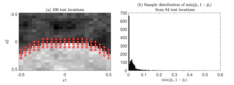
Figure 2: Empirical distribution of $\hat{p}_{i}$ for a test function over a two-dimensional grid of $(x_{1},x_{2})$ illustrated in (a).

Due to the nature of CEM inference, estimated $\hat{p}_{i}$ are highly concentrated around 0 and 1. For example, consider a test function illustrated in Figure 2 (a). In the figure, we utilize a two-dimensional grid where the output value $y(\boldsymbol{X})$ is indicated in grayscale. The test function is described in more detail momentarily in Section 3.3. Overlayed are 84 test locations as red dots. These are placed along a ridge in the response surface for dramatic effect. We set $n=20$, which means that for each test location, JGP would condition on twenty local training data examples, and consequently CEM would provide $\hat{p}_{1},\dots,\hat{p}_{n},n=20$, one for each. Figure 2 (b) shows how the $84\times 20$ values of $\hat{p}_{i}$ are distributed. In the histogram, the 95^th percentile of $\min(\hat{p}_{i},1-\hat{p}_{i})$ is around 0.1, and only 5% of $\min(\hat{p}_{i},1-\hat{p}_{i})$ is larger than 0.1, which corresponds to only one element when $n=20$.

We exploit this highly concentrated distribution of $\hat{p}_{i}$ to aggressively short-circuit the exhaustive sum (12). In so doing, we obtain a reasonable approximation because it can be shown that $\hat{p}(\boldsymbol{Z})$ quickly goes to a zero for $\boldsymbol{Z}\in\mathcal{B}_{r}(\boldsymbol{\hat{Z}})$ as $r$ increases. For example, suppose $r=1$. For $\boldsymbol{Z}\in\mathcal{B}_{1}(\boldsymbol{\hat{Z}})$, let $j$ denote the index of an element with $Z_{j}\neq\hat{Z}_{j}$ and $\min(\hat{p}_{j},1-\hat{p}_{j})$ within the 95^th percentile. Then, we have

$$\hat{p}(\boldsymbol{Z})=\hat{p}(\boldsymbol{\hat{Z}})\frac{\min(\hat{p}_{j},1-\hat{p}_{j}i)}{\max(\hat{p}_{j},1-\hat{p}_{j})}\leq\frac{0.1}{1-0.1},$$

because $\hat{p}(\boldsymbol{\hat{Z}})\leq 1$ and $\frac{\min(\hat{p}_{j},1-\hat{p}_{j}i)}{\max(\hat{p}_{j},1-\hat{p}_{j})}<0.1/(1-0.1)$. The same holds more generally, for larger $r$, where $\boldsymbol{Z}\in\mathcal{B}_{r}(\boldsymbol{\hat{Z}})$:

$$\hat{p}(\boldsymbol{Z})\leq\left(\frac{0.1}{1-0.1}\right)^{r}.$$

This value quickly decreases as $r$ increases.

Since $\hat{p}(\boldsymbol{Z})$ decreases exponentially as $r$ increases, we can obtain a good approximation to the exhaustive variance (12) by the truncated series,

$$\widehat{\operatorname*{\mathbb{V}ar}}_{R}[\mu_{J}(\boldsymbol{x}_{*})]=\frac{\sum_{r=0}^{R}\sum_{\boldsymbol{Z}\in\mathcal{B}_{r}(\boldsymbol{\hat{Z}})}s_{J}(\boldsymbol{x}_{*};\boldsymbol{Z})\hat{p}(\boldsymbol{Z})}{\sum_{r=0}^{R}\sum_{\boldsymbol{Z}\in\mathcal{B}_{r}(\boldsymbol{\hat{Z}})}\hat{p}(\boldsymbol{Z})}.$$ (14)

This expression (14) approaches the true $\operatorname*{\mathbb{V}ar}[\mu_{J}(\boldsymbol{x}_{*})]$ as $R\rightarrow n$, requiring the evaluation of $\sum_{r=0}^{R}{n\choose r}$ terms. When $R=0$, the approximation in Eq. (14) reduces to $s^{2}_{J}(\boldsymbol{x}_{*};\boldsymbol{\hat{Z}})$, which is a popular acquisition criteria in its on right, forming the basis of ALM (McKay et al., 2000), reviewed earlier in Section 1. Larger $R$-values yield only marginal gains, both in terms of the magnitude of the resulting variance estimate, and in terms of progress towards the true calculation. Again, looking ahead to our illustration coming next, our variance estimates, via Eq. (14) using $R=0$, were low by less than ten percent compared to the truth (12), specifically 9.0181 and around 10, respectively. The former improves to 9.0194 with $R=1$. We prefer $R=0$ for our empirical work later, although it’s certainly easy to try modestly larger $R$-values. Other implementation details are deferred to Section 5.

3.3 Illustration

Here we use a toy example to illustrate how the bias and variance of JGP estimates may be decomposed via the approximations laid out above. To ease visualization, we use a two-dimensional rectangular domain $[-0.5,0.5]^{2}$, which is partitioned into two regions by a curvy boundary, as illustrated in Figure 3 (a). The response function for each region is randomly drawn from an independent GP with different constant mean $\mu_{k}\in\{0,27\}$ and a squared exponential covariance function,

$$\begin{split}c(\boldsymbol{x},\boldsymbol{x}^{\prime};\theta_{k})=9\exp\left\{-\frac{1}{200}(\boldsymbol{x}-\boldsymbol{x}^{\prime})^{T}(\boldsymbol{x}-\boldsymbol{x}^{\prime})\right\}.\end{split}$$

We added an independent Gaussian noise $\mathcal{N}(0,2^{2})$ on each response value.

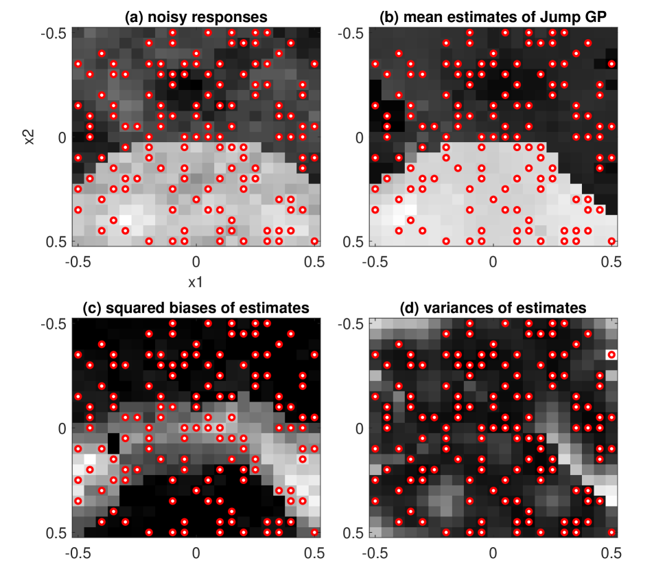
Figure 3: Bias and variances of JGP for a test function over a two-dimensional grid of $(x1,x2)$ illustrated in (a). The red dots in all figures represent the training input locations. Panel (b) shows the mean estimates from Jump GP with the training data. Panels (c) and (d) show $\widehat{\mathrm{Bias}}[\mu_{J}(\boldsymbol{x}_{*})]$ and $\widehat{\operatorname*{\mathbb{V}ar}}_{0}[\mu_{J}(\boldsymbol{x}_{*})]$ of the JGP estimates.

Figure 3 (a) shows a realization of one such surface. Overlayed are $N=132$ training inputs selected at random from a $21\times 21$ grid over the input domain. Noisy responses at those training inputs are used to estimate the JGP. Figure 3 (b) shows JGP-estimated predictive means over that grid. Figure 3 (c) and (d) show the decomposition of MSPE (7) via calculated values of $\widehat{\mathrm{Bias}}[\mu_{J}(\boldsymbol{x}_{*})]$ and $\widehat{\operatorname*{\mathbb{V}ar}}_{0}[\mu_{J}(\boldsymbol{x}_{*})]$, respectively. Observe in particular that high bias clusters around the boundary of the two regions, whereas high variance clustrs around parts of the input space where training data are sparse. The former is novel to the JGP setting, and a feature we intend to exploit next, for active learning. For JGP learning, you want more data where bias is high. The latter is a classic characteristic of (otherwise stationary) GP modeling; more data where training examples are sparse.

4 Active Learning for Jump GPs

Given training data $\mathcal{D}_{N}=\{(\boldsymbol{x}_{i},y_{i}),i=1,\ldots,N\}$, we consider an AL setup that optimizes the acquisition of new training data by selecting a tuple of input coordinates $\boldsymbol{x}_{N+1}$ among candidate positions in $\mathcal{X}_{C}$, according to some criterion. Once $\boldsymbol{x}_{N+1}$ has been selected, it is run to obtain $y_{n+1}=f(\boldsymbol{x}_{n+1})+\varepsilon$, The training data is autmented to form $\mathcal{D}_{N+1}=\mathcal{D}_{N}\cup(\boldsymbol{x}_{N+1},y_{N+1})$. Finally, the model is refit and the process repeats with $N\leftarrow N+1$. Here we develop three AL criteria for JGPs that are designed account for predictive model bias variance to varying degree.

4.1 Acquisition functions

We first consider an ALM-type criterion, selecting $\boldsymbol{x}_{N+1}$ where the MSPE (7) is maximized. Exploiging bias (11) and variance (14) estimates, we select $\boldsymbol{x}_{N+1}\in\mathcal{X}_{C}$ as

$$\begin{split}\boldsymbol{x}_{N+1}=\operatorname*{\arg\!\max}_{\boldsymbol{x}_{*}\in\mathcal{X}_{C}}\quad&\widehat{\mathrm{MSPE}}(\boldsymbol{x}_{*}),\quad\mbox{where}\\ &\widehat{\mathrm{MSPE}}(\boldsymbol{x}_{*})=\widehat{\mathrm{Bias}}[\mu_{J}(\boldsymbol{x}_{*})]^{2}+\widehat{\operatorname*{\mathbb{V}ar}}[\mu_{J}(\boldsymbol{x}_{*})].\end{split}$$ (15)

We refer to this AL critera as Maximum MSPE Acquisition.

Second, we explore an IMSPE (or ALC) type criterion that sequentially selects new data points among candidate locations in order to maximize the amount by which a new acquisition would reduce total variance throughout the input space. To evaluate how the MSPE of a JGP changes with a new data $(\boldsymbol{x}_{N+1},y_{N+1})$, we must first understand how the addition of new training data affects the $n$-nearest neighbors of a test location $\boldsymbol{x}_{*}$.

Let $R(\boldsymbol{x}_{*})=\max_{\boldsymbol{x}_{i}\in D_{n}(\boldsymbol{x}_{*})}d(\boldsymbol{x}_{*},\boldsymbol{x}_{i})$ denote the size of the neighborhood $D_{n}(\boldsymbol{x}_{*})$ before the new data is added, where $d(\cdot,\cdot)$ is Euclidean distance in $\mathcal{X}$ space. When $d(\boldsymbol{x}_{N+1},\boldsymbol{x}_{*})\geq R(\boldsymbol{x}_{*})$, the neighborhood does not change with the injection of the new data. Therefore, the change in MSPE would be zero at $\boldsymbol{x}_{*}$. Consequently, we only consider test locations $\boldsymbol{x}_{*}$ satisfying $d(\boldsymbol{x}_{N+1},\boldsymbol{x}_{*})<R(\boldsymbol{x}_{*})$ going forward. Let $\mathcal{X}(\boldsymbol{x}_{N+1})$ represent all test locations satisfying that condition. For $\boldsymbol{x}_{*}\in\mathcal{X}(\boldsymbol{x}_{N+1})$, let $\mathcal{D}_{n}(\boldsymbol{x}_{*},\boldsymbol{x}_{N+1})$ represent the new $n$-nearest neighborhood of $\boldsymbol{x}_{*}$. Without loss of generality, consider $\boldsymbol{x}_{n,*}=\operatorname*{\arg\!\max}_{\boldsymbol{x}_{i,*}\in D_{n}(\boldsymbol{x}_{*})}||\boldsymbol{x}_{*}-\boldsymbol{x}_{i,*}||$. Then, we can write

$$\mathcal{D}_{n}(\boldsymbol{x}_{*};\boldsymbol{x}_{N+1})=\mathcal{D}_{n}(\boldsymbol{x}_{*})\cup\{(\boldsymbol{x}_{N+1},y_{N+1})\}-\{(\boldsymbol{x}_{n,*},y_{n,*})\}.$$ (16)

When $(\boldsymbol{x}_{N+1},y_{N+1})$ are known, one can fit JGP to $\mathcal{D}_{n}(\boldsymbol{x}_{*};\boldsymbol{x}_{N+1})$. Let $\mu_{J}(\boldsymbol{x}_{*}|\boldsymbol{x}_{N+1},\boldsymbol{y}_{N+1})$ and $s_{J}(\boldsymbol{x}_{*}|\boldsymbol{x}_{N+1},\boldsymbol{y}_{N+1})$ denote the posterior mean and variance, based on (1). The corresponding MSPE can be achieved using (11) and (14). The corresponding MSPE is

$$\begin{split}\widehat{\mathrm{MSPE}}(\boldsymbol{x}_{*}\mid\boldsymbol{x}_{N+1},y_{N+1})=\widehat{\mathrm{Bias}}[\mu_{J}(\boldsymbol{x}_{*}\mid\boldsymbol{x}_{N+1},y_{N+1})]^{2}+\widehat{\operatorname*{\mathbb{V}ar}}[\mu_{J}(\boldsymbol{x}_{*}|\boldsymbol{x}_{N+1},y_{N+1})].\end{split}$$ (17)

In an AL setting, however, $y_{N+1}$ is unknown at the time that an acquisition decision is being made. To assess the potential value of it’s input, $\boldsymbol{x}_{N+1}$, we propose averaging over the posterior (predictive) distribution of $y_{N+1}$ based on the original data around $\boldsymbol{x}_{N+1}$, i.e., $\mathcal{D}_{n}(\boldsymbol{x}_{N+1})$. Specifically, for a JGP $Y(\boldsymbol{x}_{N+1})\mid\mathcal{D}_{n}(\boldsymbol{x}_{N+1})$ via Eq. (5) we have $p(y_{N+1}\mid\mathcal{D}_{n}(\boldsymbol{x}_{N+1}))\equiv\mathcal{N}_{1}(\mu_{J}(\boldsymbol{x}_{N+1}),\sigma^{2}+s^{2}_{J}(\boldsymbol{x}_{N+1}))$.

IMSPE may then be defined as the average MSPE over $\boldsymbol{x}_{*}$ and $y_{N+1}$,

$$\widehat{\mathrm{IMSPE}}(\boldsymbol{x}_{N+1})=\int\int\widehat{\mathrm{MSPE}}(\boldsymbol{x}_{*}\mid\boldsymbol{x}_{N+1},y_{N+1})p(y_{N+1}\mid\mathcal{D}_{n}(\boldsymbol{x}_{N+1}))d\boldsymbol{x}_{*}dy_{N+1}.$$ (18)

For acquisition, we are primarily interested in how injecting $\boldsymbol{x}_{N+1}$ into the design improves the IMSPE, which may be measured as

$$\Delta\widehat{\mathrm{IMSPE}}(\boldsymbol{x}_{N+1})=\int\Delta\widehat{\mathrm{MSPE}}(\boldsymbol{x}_{*}\mid\boldsymbol{x}_{N+1})d\boldsymbol{x}_{*},$$

where $\Delta\widehat{\mathrm{MSPE}}(\boldsymbol{x}_{*}\mid\boldsymbol{x}_{N+1})=\int\widehat{\mathrm{MSPE}}(\boldsymbol{x}_{*}\mid\boldsymbol{x}_{N+1},y_{N+1})p(y_{N+1}\mid\mathcal{D}_{n}(\boldsymbol{x}_{N+1}))dy_{N+1}-\widehat{\mathrm{MSPE}}(\boldsymbol{x}_{*})$. The term $\Delta\widehat{\mathrm{MSPE}}(\boldsymbol{x}_{*}\mid\boldsymbol{x}_{N+1})$ is non-zero only for $\boldsymbol{x}_{*}$ satisfying $d(\boldsymbol{x}_{N+1},\boldsymbol{x}_{*})<R(\boldsymbol{x}_{*})$. Let $\mathcal{X}(\boldsymbol{x}_{N+1})=\{\boldsymbol{x}_{*}\in\mathcal{X},d(\boldsymbol{x}_{N+1},\boldsymbol{x}_{*})<R(\boldsymbol{x}_{*})\}$ represent the set of such test locations. The improvement can be further refined to

$$\Delta\widehat{\mathrm{IMSPE}}(\boldsymbol{x}_{N+1})=\int_{\mathcal{X}(\boldsymbol{x}_{N+1})}\Delta\widehat{\mathrm{MSPE}}(\boldsymbol{x}_{*}\mid\boldsymbol{x}_{N+1})d\boldsymbol{x}_{*}.$$

Unfortunately, this integral is not available in closed form, but have found that it can be approximated accurately using Monte Carlo-based quadrature. First draw $\boldsymbol{x}_{*}$ uniformly over $\mathcal{X}$. If $\boldsymbol{x}_{*}\in\mathcal{X}(\boldsymbol{x}_{N+1})$, draw i.i.d. samples of $y_{N+1}$ from $p(y_{N+1}\mid\mathcal{D}_{n}(\boldsymbol{x}_{N+1}))$ to evaluate the integral in $\Delta\widehat{\mathrm{MSPE}}(\boldsymbol{x}_{*}|\boldsymbol{x}_{N+1})$. Finally, repeat to accumulate averages of $\Delta\widehat{\mathrm{MSPE}}(\boldsymbol{x}_{*}\mid\boldsymbol{x}_{N+1})$ to approximate $\Delta\widehat{\mathrm{IMSPE}}(\boldsymbol{x}_{N+1})$. Selecting $\boldsymbol{x}_{N+1}=\operatorname*{\arg\!\min}_{\boldsymbol{x}_{*}\in\mathcal{X}_{C}}\Delta\widehat{\mathrm{IMSPE}}(\boldsymbol{x}_{N+1})$ in this way yields what we dub a Minimum IMSPE Acquisition.

Our final AL criteria is Maximum Variance Acquisition

$$\boldsymbol{x}_{N+1}=\operatorname*{\arg\!\max}_{\boldsymbol{x}_{*}\in\mathcal{X}_{C}}\quad\widehat{\operatorname*{\mathbb{V}ar}}[\mu_{J}(\boldsymbol{x}_{*})].$$ (19)

Like the first criteria, above, this is an ALM-type, but one which ignores predictive bias. Focusing exclusively on variance which is known to produce space-filling designs. Consequently, it serves as a straw-man, or baseline in order to calibrate our empirical experiments and illustrations against a sensible benchmark.

4.2 Illustration

Here we use a simple toy example to explore the three acquisition functions presented in the previous section. For effective visualization, we use a two-dimensional rectangular domain $[0,2]^{2}$.

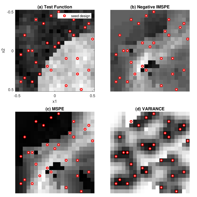
Figure 4: Three acquisition functions evaluated over a $21\times 21$ testing grid. Panel (a) shows the data. Panels (b)-(d) show -$\widehat{\mathrm{IMSPE}}(\boldsymbol{x}_{*})$, $\widehat{\mathrm{MSPE}}(\boldsymbol{x}_{*})$ and $\widehat{\operatorname*{\mathbb{V}ar}}[\mu_{J}(\boldsymbol{x}_{*})]$, respectively.

In Figure 4 (a) this domain is partitioned into two regions, $\mathcal{X}_{1}$ (lighter shading) and $\mathcal{X}_{2}$ (darker). The noisy response function for each region is randomly drawn from an independent GP with the same regional means and covariance functions used in our Section 3.3 illustration plus additive independent Gaussian noise with $\sigma=2$. AL is initialized with thirty seed-data positions via LHD, and these are overlayed onto all panels of the figure. Given noisy observations at these seed positions, we evaluated our three AL criteria on $21\times 21$ grid of candidates $\mathcal{X}_{C}$ in the input domain. Figure 4 (b)–(d) provides visuals for their values in greyscale. For example, the maximum variance criterion in (d) indicates $\widehat{\operatorname*{\mathbb{V}ar}}[\mu_{J}(\boldsymbol{x}_{*})]$. Observe that this criteria is inversely proportional to the positions (and densities, locally) of seed data. This criteria exhibits behavior similar to conventional variance-based criteria (such as ALM or ALC) derived from stationary GPs. One slight difference, however, is that that the variance of JGP is slightly higher around regional boundaries, compared to an ordinary stationary GP. Around the boundaries, local data is bisected, and only one section is used for JGP prediction, which makes the variance elevated around the boundaries. Later, in Figure 5, we will see that slightly more data positions are selected around regional boundaries with the variance criterion. As shown in panels (b) and (c), the negative IMSPE and MSPE values consider model bias and variance. Around regional boundaries, bias values dominate variance estimates. Therefore, as we will show in Figure 5, data acquisitions are highly concentrated around regional boundaries.

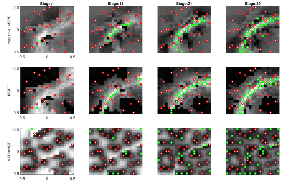
Figure 5: Active selection of design points for three acquisition functions. Dots represent seed designs, and boxes represent the design points added by active learning.

Future acquisitions further differentiate themselves according to the heuristic in question. For the same toy example, we ran AL for each choice of the three acquisition functions: start with a seed design of 30 random LHD data points; subsequently add one additional design point every AL stage for 30 stages. Figure 5 shows how the acquisition function values change as the AL stages progress and how they affect the selection training data inputs. For the IMSPE and MSPE criteria, the selected positions are highly concentrated around regional boundaries. With the variance criterion, the positions are close to a uniform distribution with a mild degree of concentration around the regional boundary.

To explore accuracy of JGP under these three AL regimes, we conducted the Monte Carlo experiment in 100 replications. Each of these follows the same format as above, augmented to track JGP out-of-sample MSPE along the way in two variations. The first involves a testing set comprising of the 441 locations on the $21\times 21$; the second contains only the 82 closest of those locations to the regional boundary. We also perform the paired Wilcoxon test to check statistical significance of the comparison.

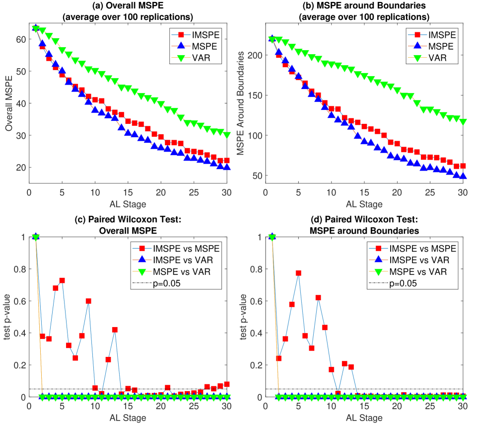
Figure 6: MSPE of JGP for different stages of active learning. The top panels show the average MSPE over 100 replicated experiments. The bottom panels show the p-values of the paired Wilcoxon test for statistical significance.

The left panels of Figure 6 report the overall MSPE with the first set, and the right panels report the MSPE near the regional boundary. The MSPE values near the regional boundary are more distinct among the three criteria than the overall MSPE. The overall MSPE are more distinct in the middle around the AL stage 15, and the gaps saturate in the later stages as data points become denser. The distinction between AL Stages 15 and 25 is statistically significant with confidence level 95%. Using the maximum MSPE criterion achieves the best overall MSPE for all stages. The maximum MSPE criterion is also the most effective in reducing the MSPE near the regional boundary. Overall, the MSPE criterion is most preferred, based on the accuracy metrics and its computation speed (e.g. computation time for IMSPE is 0.12 seconds versus 0.07 seconds for MSPE) for this toy example.

5 Empirical benchmarking and validation

In this section, we use one toy example and two real experiments to validate the proposed AL strategies for the JGP. Our metrics include out-of-sample mean-squared error (MSE, smaller is better) and the negative log posterior score (Gneiting & Raftery, 2007, Eq. 25), which is proportional to the predictive Gaussian log likelihood (NLPD, smaller is better). We check how the two criteria change as more data are injected via AL.

As benchmarks, we compare the JGP/MSPE, the proposed active learning of JGP with the MSPE criterion, with two existing non-stationary GP models and their associated ALC criterion: Treed GP/ALC (Gramacy & Lee, 2008) and two-layer Deep GP/ALC (Sauer et al., 2020). We use the tgp package (Gramacy & Taddy, 2016) for the former; and deepgp (Sauer, 2022) for the latter. Together, these options span the space of established methodology for AL and nonstationary surrogate modeling via partitioning/hard breaks and smoothly evolving regime changes, respectively. We note that, on the size of problems we entertain, the deepgp implementation is slow. Consequently, we limited the number of MCMC iterations to 1,000 burn-in, and 2,000 total and the squared-exponential kernel. Otherwise, package defaults were used throughout.

Our implementation of the JGP, and the associated AL subroutines introduced in this manuscript, may be downloaded from the author’s website: https://www.chiwoopark.net/code-and-dataset. Here too we use the defaults suggested by the software documentation. For example, we set the local data size to $n=15$. Our analysis here focuses on the MSPE AL criterion for JGP in order to reduce clutter. Practitioners can simply change the criterion option parameter to try with IMSPE or pure variance. We report that results with IMSPE are similar to what is shown here.

5.1 Synthetic Example

We begin with simple toy example in a 2d rectangular domain $[0,2]^{2}$, which is partitioned into two regions: $\mathcal{X}_{1}$ (lighter shading in the visuals, e.g., Figure 8) and $\mathcal{X}_{2}$ (darker shading). The response function for each region is

$$\begin{split}f(x_{1},x_{2})=\sum_{k=1}^{K}\left\{\sin\left(\frac{x_{1}}{0.4}\right)\cos\left(\frac{x_{2}}{0.4}\right)+3\times 1_{\mathcal{X}_{2}}(\boldsymbol{x})\right\}.\end{split}$$

We randomly generate a seed training dataset of size $N=44$ following a LHD. The corresponding noisy response variables follow $f(x_{i1},x_{i2})$ plus Gaussian noise with zero mean and $\sigma=0.4$. Subsequently, thirty stages of AL acquisition are performed, separately for our three comparators: JGP/MSPE, TGP/ALC and DGP/ALC.

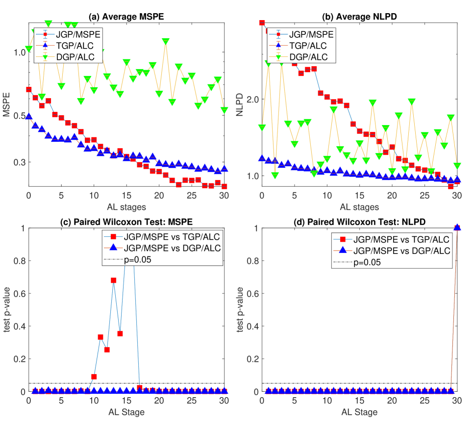
Figure 7: MSPE and NLPD of JGP/MSPE, TGP/ALC and DGP/ALC. The plots are based on a sequential learning with 44 seed experiments and 30 additional AL acquisitions. The values reported are based on 100 MC repetitions.

We compare JGP/MSPE with TGP/ALC and DGP/ALC. Figure 7 shows the trend of MSE and NLPD as AL progresses. The top panels report the average over 100 MC replications. The bottom panels report the statistical significance based on paired Wilcoxon tests. The MSPE and NLPD of DGP/ALC fluctuates, not showing decreasing trends while more data are being added by AL. Based on the visual inspection of its prediction from Figure 8, the DGP is struggling both with the small amount of training data, and with high variability owing to the small MCMC. Results for TGP, by contrast, are more stable and more accurate. However, again the data set is too small for axis-aligned partitioning to isolate the boundary between the two regions. Predictions resemble the true response surface, but huge prediction errors occur around the regional boundary. Eventually, TGP is able to make a one-level tree split, as illustrated by the “AL$-$Stage = 20” summary of Figure 8.

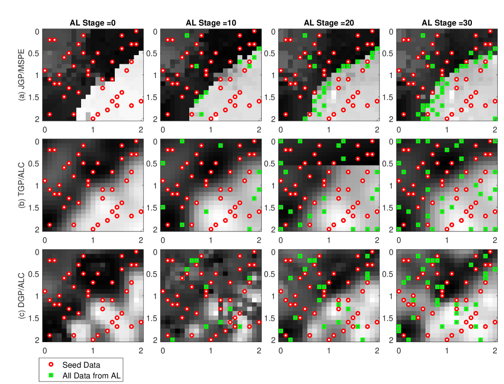
Figure 8: Predictions from JGP/MSPE, TGP/ALC and DGP/ALC. Stage 0 involves 44 seed experiments from LHD. One data point is added every AL stage for 30 stages. The test locations are selected as a $21\times 21$ uniform grid over $[0,2]\times[0,2]$ domain.

However, this one-level split offers a poor approximation to the curvy regional boundary. Finally, the JGP predictions are closest to the true response surface, allocating data resources around the regional boundary versus an almost uniform placing of data points from TGP/ACL and DGP/ALC. Although it is somewhat slower to “get started” than TGP/ALC, eventually results in Figure 7 reveal JGP/MSPE as the clear winner of the comparison. These gains are statistically significant after AL stage 15.

5.2 Performance of a smart factory system in 4d

This numerical example comes with relatively large sample size and large variability in the response variable. It also has a higher input dimension than the previous example. Figure 9(a) depicts an automated material handling system (AMHS) in a semiconductor manufacturing facility. The AMHS uses autonomous vehicles running on overhead rails optimize material flow and to transfer silicon wafers between wafer fabrication steps. The AMHS aims to maintain high delivery speeds and keep low levels of human-related intervention and contamination. It has been observed that the AMHS becomes a major bottleneck in the fabrication process as the wafer production level increases (Siebert et al., 2018).

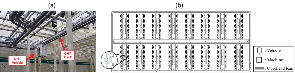
Figure 9: Simulated layout of automated material handling system. Part (a) is a reprint of Hwang & Jang (2020, Figure 1) under License CC BY-NC-ND 4.0.

Fab operators widely use simulation to optimize design and operational policies under various AMHS operating scenarios (Kang et al., 2022). Here we use a high-fidelity computer simulation model to evaluate the performance of AMHS under various design configurations. The simulation consists of 200 autonomous vehicles running on the layout of overhead rails depicted diagrammatically in Figure 9 (b).

A key performance metric associated with AMHS is the waiting time until an autonomous vehicle is finally assigned to serve a transfer request. Since the relationship between vehicle specifications and the performance metrics is of great interest (Yang et al., 1999), we consider three design variables that are thought to affect this waiting time: vehicle acceleration, vehicle speed, and the required minimum distance between vehicles. We also consider one operational design variable: the maximum search range of empty vehicles in a distance-based vehicle dispatching policy. The policy aims to reduce the mean and variation of empty travel time. It is desirable to optimize the maximum search range of empty vehicles by controlling the trade-off between the idle time and empty travel time of vehicles. These design variables and sensible ranges are summarized in Table 1.

Design Variables	Minimum	Maximum
vehicle acceleration (meters/second2)	0.25	5.0
vehicle speed (meters/second)	2.5	3.5
required minimum distance between vehicles (meters)	0.25	1
maximum search range of empty vehicles (meters)	30	500

Table 1: Design variables for AMHS simulations.

Preliminary experiments revealed that transfer waiting times are almost zero under most normal operating conditions, but can suddenly jump to significant levels as those conditions transition into “heavy traffic” situations. We posit that JGP with AL is a suitable approach to learn these jumping behaviors. Here we perform batch acquisition in order to leverage a distributed supercomputing resource for model runs, with ten runs per batch. The campaign begins with a seed experiment of size $N=500$, via LHD, which is comparable to considering five different levels for each of the four factors if a simple grid design is used. We then ran 30 AL stages, after which both MSPE and NLPD improve only marginally.

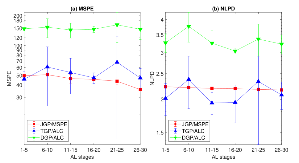
Figure 10: MPSE and NLPD over five stages of JGP/MSPE versus GP/ALC with simulated experiments for a smart factory system. The GP/MSPE curve represents the benchmark performance of local GP when the data selections are given by our proposed approach.

The outcome of this experiment exhibits large variability. Accordingly, both MSPE and NLPD metrics fluctuate substantially over AL stages. To illustrate, we segmented the 30 AL stages into six groups of five: Stages 1 to 5, Stages 6 to 10, …, Stages 25 to 30. We then report the average and standard deviation of the MSPE and NLPD values within each of the six groups. Figure 10 shows the grouped metrics for JGP/MSPE versus two benchmarks: TGP/ALC and DGP/ALC.

For the early AL stages, both TGP/ALC and JGP/MSPE work comparably in MSPE, while DGP/ALC has much higher MSPE values. We observe that the response variable of this example is split into two regions by a linear boundary. This regime change can be effectively modeled by all of JGP, TGP and DGP. Therefore, TGP and JGP with initial seed designs work comparably. DGP’s poor performance is mainly due to a relatively small training data size. As the AL stages progress, the MSPE of JGP/MSPE shows a downward trend from 50 to 35, and the NLPD also goes down from 2.2309 to 2.1698. We acknowledge that the NLPD improvement of JGP/MSPE is not as good as its MSPE. This is because JGP somewhat underestimates the large variability for this example. The MSPEs and NLPDs of TGP/ALC and DGP/ALC go up and down with no clear improvement or trend.

It is worth remarking on the variability of observed MSPE and NLPD values in the sequential study. TGP/ALC exhibits substantially larger swings over AL stages, as evidenced by the long error bars in Figure 10, while the JGP/MSPE has shown much smaller variability. Such large variability is one of the distinct characteristics of the partitioned based models like TGP. Compared to that, JGP’s variability is mild.

5.3 Prediction of carbon nanotube yield in 2d

Here we present an application of the proposed JGP-AL strategy to a materials research problem, illustrating the applicability of the new approach. Due to high experimental expense, we can only illustrate how the new approach is applied to this real application. Our experimental budged did not allow us to benchmark against our other comparators.

Our colleagues at the Air Force Research Lab (AFRL) developed an autonomous research experimentation system (ARES) for carbon nanotubes (Nikolaev et al., 2016). ARES is a robot capable of performing closed-loop iterative materials experimentation, carbon nanotube processing and ultimately measuring in-line process yield. Here, we utilize ARES to map out carbon nanotube yields as a function of two input conditions: reaction temperature and the log ratio of an oxidizing chemical concentration and a reducing chemical concentration. In previous experiments it was observed that nanotube yields are almost zero in certain growth conditions. Then suddenly, when those conditions approach a regime where they become more activated, yield “jumps” up to a substantial level. These activating conditions vary significantly depending on how the two inputs we varied.

The ARES system is designed to run multiple experiments in parallel which is amenable to AL in batches. We started with $N=25$ seed experiments, via LHD, and sequentially added batches of five new runs over AL stages. The number of such stages is determined algorithmically by checking when the percentage improvements of MSPE and NLPD drops to less than 3%. Based on that stopping rule, we ran a total five AL stages, which ultimately doubled the size of the seed experiment. Selection of each batch was performed by iteratively deploying single-point acquisition, followed by imputing the missing output with the predictive mean furnished by the JGP.

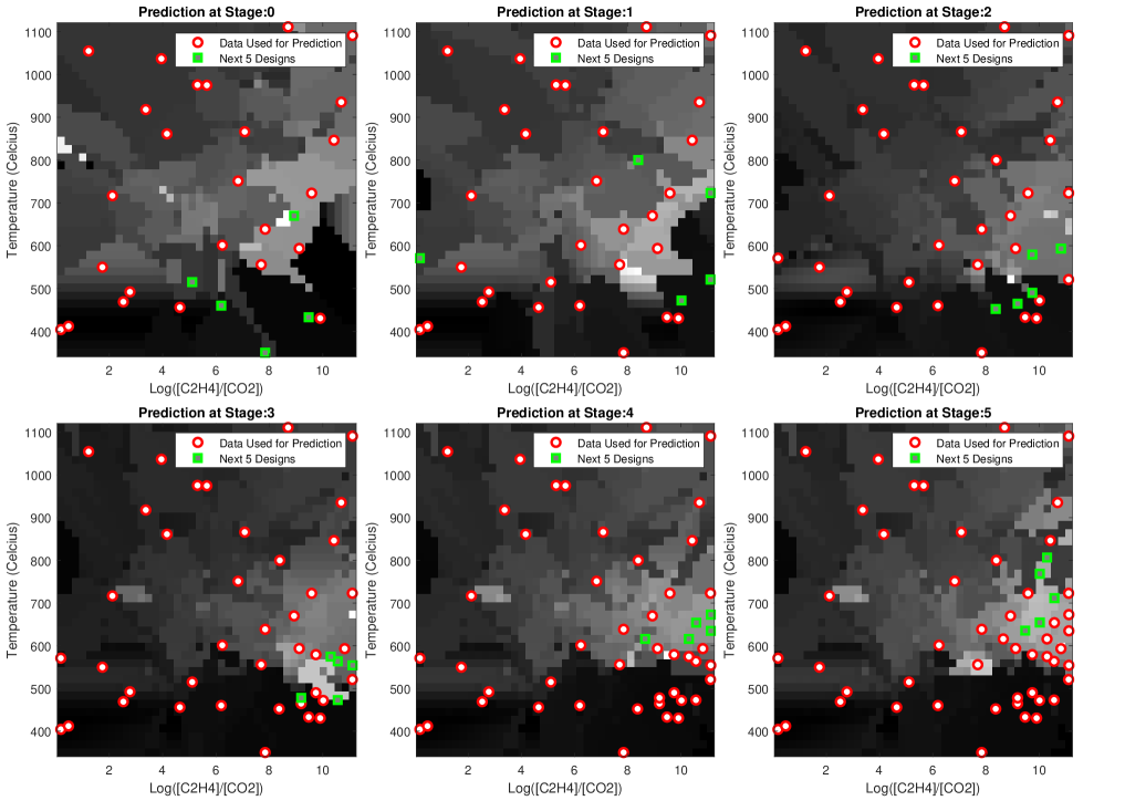
Figure 11: Active Learning of CNT Yield with JGP/MSPE. AL Stage 0 comes with 25 seed experiments from LHD, and each AL stage adds five more experimental data.

Figure 11 shows the results from the seed stage (Stage 0) and the subsequent five AL batches (Stages 1, 2, …, 5). Each panel shows the JGP mean prediction realized out-of-sample over a rectangular input domain $[0,11]\times[300,1100]$ after training on the data acquired up to the respective stage. Here, we limit the size of the candidate pool $\mathcal{X}_{C}$ to 500. Therefore, selections do not necessarily comprise of top five values of bias-plus-variance estimates over the entire domain, but they seem to work well regardless. Observe from the figure that the first two stages are highly exploratory, with new acquisitions spread out more widely. In later stages, acquisitions focus on the likely location of a jump in yield output. The high degree of concentration of data acquisitions on the right bottom of the study space is also explained by the magnitude of yield jumps around that area. Although there are yield jumps in other locations, the magnitude of those jumps are mild by comparison. The area in the bottom-right, of highest concentration of AL acquisition, is consistent with our AFRL colleague’s expert judgment on high yield regions. Through this experimental exploration, we found that the best growth region occurs along the jump boundary. Runs above the jump result in less nanotube growth, so being able to identify the jump spline is of greater value than than a binary growth/no growth determination.

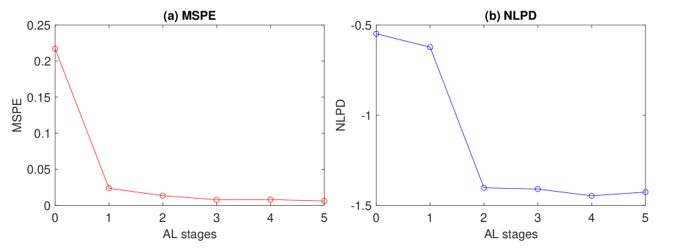
Figure 12: Carbon nanotube MSPE and NLPD over five AL stages of JGP/MSPE batch acquisition.

Figure 12 provides quantitative results summarizing each stage of AL acquisition out-of-sample, via MSPE and NLPD, based on the yield obtained from fifty additional LHD experiments. In the first two AL stages, MSPE improves significantly, and afterwards there is a steady decline as acquisition become more concentrated on important regions of nanotube growth. Observe that NLPD, combining accuracy and uncertainty quantification, steadily decreases throughout. After the fourth stage, both MSPE and NLPD statistics stabilized, triggering our threshold and stopping the AL campaign.

6 Conclusion

We explored the Jump Gaussian process (JGP) model as a surrogate for piecewise continuous response surfaces. We studied estimates of predictive bias and variance for the JGPs with an eye toward developing an effective active learning (AL) heuristic for the the model. We showed that JGP bias is largely influenced by the accuracy of the classifier governing regimes learned by the JGP, whereas model variance is comparable to that of the standard GP model. Consequently, to reduce model bias and variance together we should invest more data points (via AL) around boundaries between regimes, while otherwise continuing to place data points around less populated areas of a design space. Based on that principle, we introduced three AL criteria: one minimizing the integrated mean squared prediction error (IMSPE), another placing points at the peak of the mean squared prediction error (MSPE), and the last one placing at the peak of the predictive variance.

We evaluated these three criteria using various simulation scenarios by tracking the changes in mean square prediction error (MSPE) and negative log posterior density (NLPD) metrics. Based on a preliminary synthetic benchmarking exercise, we determined that MSPE offered best efficiency trade-off. We compared JGP with MSPE criterion to existing non-stationary GP models and their associated ALC criterion, including a deep GP with ALC and a Bayesian treed GP with ALC. The proposed JGP/MSPE outperformed these comparators.

Finally, we illustrated our methods on two real experiments. Our first example involved a study of the performance of an autonomous material handling system in smart factory facilities. The JGP/MSPE method achieves high estimation accuracy with low computational costs and low variability compared to our benchmarks. In the second experiment we highlighted a real materials design application of the proposed method for effectively mapping carbon nanotube yield as a function of two design variables.

ACKNOWLEDGMENTS

We acknowledge support for this work. Park and Gramacy are supported by the National Science Foundation (NSF-2152655, NSF-2152679). Waelder and Maruyama are supported by the Air Force Office of Scientific Research (LRIR-19RXCOR040). Kang and Hong are partially supported by the National Research Foundation of Korea (NRF-2020R1A2C2004320) and by the BK21 FOUR of the National Research Foundation of Korea (NRF-5199990914451). The main algorithm of this work is protected by a provisional patent pending with application number 63/386,823.

References

- (1)
- Abrahamsen (1997) Abrahamsen, P. (1997), ‘A review of Gaussian random fields and correlation functions’, Norsk Regnesentral/Norwegian Computing Center Oslo, https://www.nr.no/directdownload/917_Rapport.pdf.
- Beck & Guillas (2016) Beck, J. & Guillas, S. (2016), ‘Sequential design with mutual information for computer experiments (MICE): Emulation of a tsunami model’, SIAM/ASA Journal on Uncertainty Quantification 4(1), 739–766.
-
Binois et al. (2018)
Binois, M., Gramacy, R. & Ludkovski, M. (2018), ‘Practical heteroscedastic Gaussian process
modeling for large simulation experiments’, Journal of Computational and
Graphical Statistics 27(4), 808–821.
https://doi.org/10.1080/10618600.2018.1458625 -
Binois et al. (2019)
Binois, M., Huang, J., Gramacy, R. & Ludkovski, M. (2019), ‘Replication or exploration? Sequential design for
stochastic simulation experiments’, Technometrics 27(4), 808–821.
https://doi.org/10.1080/00401706.2018.1469433 - Bryant & Williamson (1978) Bryant, P. & Williamson, J. A. (1978), ‘Asymptotic behaviour of classification maximum likelihood estimates’, Biometrika 65(2), 273–281.
- Cohn et al. (1996) Cohn, D. A., Ghahramani, Z. & Jordan, M. I. (1996), ‘Active learning with statistical models’, Journal of Artificial Intelligence Research 4(1), 129–145.
- Damianou & Lawrence (2013) Damianou, A. & Lawrence, N. D. (2013), Deep Gaussian processes, in C. M. Carvalho & P. Ravikumar, eds, ‘Proceedings of the Sixteenth International Conference on Artificial Intelligence and Statistics’, Vol. 31 of Proceedings of Machine Learning Research, PMLR, Scottsdale, Arizona, USA, pp. 207–215.
- Dempster et al. (1977) Dempster, A., Laird, N. & Rubin, D. (1977), ‘Maximum likelihood from incomplete data via the em algorithm’, Journal of the Royal Statistical Society 39(1), 1–38.
- Gneiting & Raftery (2007) Gneiting, T. & Raftery, A. E. (2007), ‘Strictly proper scoring rules, prediction, and estimation’, Journal of the American Statistical Association 102(477), 359–378.
- Gramacy (2020) Gramacy, R. B. (2020), Surrogates: Gaussian Process Modeling, Design, and Optimization for the Applied Sciences, CRC Press, Boca Raton, FL, USA.
- Gramacy & Apley (2015) Gramacy, R. B. & Apley, D. W. (2015), ‘Local Gaussian process approximation for large computer experiments’, Journal of Computational and Graphical Statistics 24(2), 561–578.
- Gramacy & Lee (2009) Gramacy, R. B. & Lee, H. K. (2009), ‘Adaptive design and analysis of supercomputer experiments’, Technometrics 51(2), 130–145.
- Gramacy & Lee (2008) Gramacy, R. B. & Lee, H. K. H. (2008), ‘Bayesian treed Gaussian process models with an application to computer modeling’, Journal of the American Statistical Association 103(483), 1119–1130.
- Gramacy et al. (2014) Gramacy, R., Niemi, J. & Weiss, R. (2014), ‘Massively parallel approximate Gaussian process regression’, SIAM/ASA Journal on Uncertainty Quantification 2(1), 564–584.
-
Gramacy & Taddy (2016)
Gramacy, R. & Taddy, M. (2016),
tgp: Bayesian Treed Gaussian Process Models.
R package version 2.4-14.
https://CRAN.R-project.org/package=tgp - Gupta & Chen (2010) Gupta, M. R. & Chen, Y. (2010), ‘Theory and use of the EM algorithm’, Foundations and Trends in Signal Processing 4(3), 223–296.
- Hastie et al. (2009) Hastie, T., Tibshirani, R. & Friedman, J. (2009), The elements of statistical learning: data mining, inference, and prediction, Springer, New York, NY.
- Heaton et al. (2017) Heaton, M. J., Christensen, W. F. & Terres, M. A. (2017), ‘Nonstationary Gaussian process models using spatial hierarchical clustering from finite differences’, Technometrics 59(1), 93–101.
- Hwang & Jang (2020) Hwang, I. & Jang, Y. J. (2020), ‘Q () learning-based dynamic route guidance algorithm for overhead hoist transport systems in semiconductor fabs’, International Journal of Production Research 58(4), 1199–1221.
- Kang et al. (2022) Kang, B., Park, C., Kim, H. & Hong, S. (2022), ‘Bayesian optimization for the vehicle dwelling policy in a semiconductor wafer fab’, IEEE Transactions on Automation Science and Engineering submitted, 1–21.
- Kim et al. (2005) Kim, H.-M., Mallick, B. K. & Holmes, C. C. (2005), ‘Analyzing nonstationary spatial data using piecewise Gaussian processes’, Journal of the American Statistical Association 100(470), 653–668.
- Konomi et al. (2014) Konomi, B. A., Sang, H. & Mallick, B. K. (2014), ‘Adaptive Bayesian nonstationary modeling for large spatial datasets using covariance approximations’, Journal of Computational and Graphical Statistics 23(3), 802–829.
- Krause et al. (2008) Krause, A., Singh, A. & Guestrin, C. (2008), ‘Near-optimal sensor placements in Gaussian processes: Theory, efficient algorithms and empirical studies’, Journal of Machine Learning Research 9(Feb), 235–284.
- Lam & Notz (2008) Lam, C. Q. & Notz, W. (2008), ‘Sequential adaptive designs in computer experiments for response surface model fit’, Statistics and Applications 6(1), 207–233.
- Lin & Tang (2015) Lin, C. & Tang, B. (2015), ‘Latin hypercubes and space-filling designs’, Handbook of Design and Analysis of Experiments pp. 593–625.
- Luo et al. (2021) Luo, Z., Sang, H. & Mallick, B. (2021), ‘A Bayesian contiguous partitioning method for learning clustered latent variables’, Journal of Machine Learning Research 22, 1–52.
- Magrez et al. (2010) Magrez, A., Seo, J. W., Smajda, R., Mionić, M. & Forró, L. (2010), ‘Catalytic CVD synthesis of carbon nanotubes: towards high yield and low temperature growth’, Materials 3(11), 4871–4891.
- Malloy & Nowak (2014) Malloy, M. L. & Nowak, R. D. (2014), ‘Near-optimal adaptive compressed sensing’, IEEE Transactions on Information Theory 60(7), 4001–4012.
- McKay et al. (2000) McKay, M. D., Beckman, R. J. & Conover, W. J. (2000), ‘A comparison of three methods for selecting values of input variables in the analysis of output from a computer code’, Technometrics 42(1), 55–61.
- Mitchell (1997) Mitchell, T. (1997), Machine Learning, McGraw-Hill, Inc, New York, NY.
- Mu et al. (2017) Mu, R., Dai, L. & Xu, J. (2017), ‘Sequential design for response surface model fit in computer experiments using derivative information’, Communications in Statistics - Simulation and Computation 46(2), 1148–1155.
- Nikolaev et al. (2016) Nikolaev, P., Hooper, D., Webber, F., Rao, R., Decker, K., Krein, M., Poleski, J., Barto, R. & Maruyama, B. (2016), ‘Autonomy in materials research: A case study in carbon nanotube growth’, npj Computational Materials 2, 16031.
- Paciorek & Schervish (2006) Paciorek, C. & Schervish, M. (2006), ‘Spatial modelling using a new class of nonstationary covariance functions’, Environmetrics 17(5), 483–506.
- Park (2022) Park, C. (2022), ‘Jump Gaussian process model for estimating piecewise continuous regression functions’, Journal of Machine Learning Research 23(278), 1–37.
-
Park et al. (2023)
Park, C., Qiu, P., Carpena-Núñez, J., Rao, R., Susner, M. & Maruyama, B. (2023), ‘Sequential adaptive
design for jump regression estimation’, IISE Transactions 55(2), 111–128.
https://doi.org/10.1080/24725854.2021.1988770 - Pope et al. (2021) Pope, C. A., Gosling, J. P., Barber, S., Johnson, J. S., Yamaguchi, T., Feingold, G. & Blackwell, P. G. (2021), ‘Gaussian process modeling of heterogeneity and discontinuities using Voronoi tessellations’, Technometrics 63(1), 53–63.
- Rasmussen & Williams (2006) Rasmussen, C. & Williams, C. (2006), Gaussian Processes for Machine Learning, MIT Press, Cambridge, MA.
- Salimbeni & Deisenroth (2017) Salimbeni, H. & Deisenroth, M. (2017), Doubly stochastic variational inference for deep Gaussian processes, in I. Guyon, U. V. Luxburg, S. Bengio, H. Wallach, R. Fergus, S. Vishwanathan & R. Garnett, eds, ‘Advances in Neural Information Processing Systems’, Vol. 30, Long Beach, CA, USA.
- Sampson & Guttorp (1992) Sampson, P. & Guttorp, P. (1992), ‘Nonparametric estimation of nonstationary spatial covariance structure’, Journal of the American Statistical Association 87(417), 108–119.
- Santner et al. (2018) Santner, T., Williams, B. & Notz, W. (2018), The Design and Analysis of Computer Experiments, Second Edition, Springer–Verlag, New York, NY.
- Sauer (2022) Sauer, A. (2022), deepgp: Sequential Design for Deep Gaussian Processes using MCMC. R package version 1.0.0.
- Sauer et al. (2020) Sauer, A., Gramacy, R. B. & Higdon, D. (2020), ‘Active learning for deep Gaussian process surrogates’, arXiv preprint arXiv:2012.08015 .
- Schmidt & O’Hagan (2003) Schmidt, A. & O’Hagan, A. (2003), ‘Bayesian inference for non-stationary spatial covariance structure via spatial deformations’, Journal of the Royal Statistical Society: Series B 65(3), 743–758.
- Siebert et al. (2018) Siebert, M., Bartlett, K., Kim, H., Ahmed, S., Lee, J., Nazzal, D., Nemhauser, G. & Sokol, J. (2018), ‘Lot targeting and lot dispatching decision policies for semiconductor manufacturing: optimisation under uncertainty with simulation validation’, International Journal of Production Research 56(1-2), 629–641.
- Taddy et al. (2011) Taddy, M. A., Gramacy, R. B. & Polson, N. G. (2011), ‘Dynamic trees for learning and design’, Journal of the American Statistical Association 106(493), 109–123.
- Wendland (2004) Wendland, H. (2004), Scattered Data Approximation, Cambridge University Press, Cambridge, England.
- Yang et al. (1999) Yang, T., Rajasekharan, M. & Peters, B. A. (1999), ‘Semiconductor fabrication facility design using a hybrid search methodology’, Computers & Industrial Engineering 36(3), 565–583.