CHIME/FRB Discovery of 25 Repeating Fast Radio Burst Sources

Abstract

We present the discovery of 25 new repeating fast radio burst (FRB) sources found among CHIME/FRB events detected between 2019 September 30 and 2021 May 1. The sources were found using a new clustering algorithm that looks for multiple events co-located on the sky having similar dispersion measures (DMs). The new repeaters have DMs ranging from $\sim$220 pc cm^-3 to $\sim$1700 pc cm^-3, and include sources having exhibited as few as two bursts to as many as twelve. We report a statistically significant difference in both the DM and extragalactic DM (eDM) distributions between repeating and apparently nonrepeating sources, with repeaters having lower mean DM and eDM, and we discuss the implications. We find no clear bimodality between the repetition rates of repeaters and upper limits on repetition from apparently nonrepeating sources after correcting for sensitivity and exposure effects, although some active repeating sources stand out as anomalous. We measure the repeater fraction over time and find that it tends to an equilibrium of $2.6_{-2.6}^{+2.9}$% over our total time-on-sky thus far. We also report on 14 more sources which are promising repeating FRB candidates and which merit follow-up observations for confirmation.

1 Introduction

Fast radio bursts (FRBs) are microsecond–millisecond flashes of radio waves that are detectable over extragalactic distances (see Cordes & Chatterjee, 2019; Petroff et al., 2019, for reviews of the phenomenon). Some FRB sources repeat, which rules out cataclysmic models for burst production (Spitler et al., 2016). Magnetars are likely to be the origin of at least a fraction of FRBs as the two source classes have been directly linked (Bochenek et al., 2020; CHIME/FRB Collaboration et al., 2020a). The sources that repeat show clustered activity (Oppermann et al., 2018) that in some cases is periodic, with bursts being detectable only during a window of time in each cycle (CHIME/FRB Collaboration et al., 2020b; Rajwade et al., 2020; Cruces et al., 2021). For one source, this periodic activity has been shown to be chromatic, with activity at lower frequencies trailing the activity at higher frequencies (Pastor-Marazuela et al., 2021; Pleunis et al., 2021a; Bethapudi et al., 2022). Importantly, it is as-yet unclear whether all FRBs repeat (Caleb et al., 2019; James et al., 2020a, b), what fraction of repeating sources show periodic activity, and on what timescales repeaters are active.

Complex time-frequency structure, with subbursts that drift downward in frequency as time progresses, seems ubiquitous among bursts from repeating sources (Hessels et al., 2019; CHIME/FRB Collaboration et al., 2019a). On average, repeater bursts are observed to be longer in duration and narrower in bandwidth than for bursts seen from nonrepeating sources (Pleunis et al., 2021b). It is unclear if this observed difference represents an intrinsic difference in the two populations, if it is caused by a propagation effect related to distinct source environments, or if it is due to a selection effect that leads to the observation of two extremes out of a continuum of source properties (e.g., Connor et al., 2020).

Repeating sources of FRBs provide the best opportunity for detailed follow-up observations, and the most prolific of repeaters – FRB 20121102A (Spitler et al., 2016), FRB 20180916B (CHIME/FRB Collaboration et al., 2019b), FRB 20190520B (Niu et al., 2022), FRB 20200120E (Bhardwaj et al., 2021a), and FRB 20201124A (Lanman et al., 2022) – have provided many insights. All five have been localized to sub-arcsecond precision. They are associated with a star-forming dwarf galaxy, a disk galaxy, another star-forming dwarf galaxy, a globular cluster, and a barred galaxy, respectively (Tendulkar et al., 2017; Marcote et al., 2020; Niu et al., 2022; Kirsten et al., 2022; Xu et al., 2022), demonstrating that repeaters inhabit a variety of host types. Two sources of repeating FRBs that live in extreme magneto-ionic environments are coincident with persistent radio sources (PRSs; Michilli et al., 2018; Niu et al., 2022) but for other sources, PRSs of luminosity similar to these two have been ruled out (Law et al., 2022). The complex magnetized environments of repeaters can result in depolarization of bursts towards lower frequencies (Feng et al., 2022), depolarization due to Faraday conversion (Kumar et al., 2022) and temporal evolution of the Faraday rotation that can be secular (Hilmarsson et al., 2021), a combination of stochastic and secular (Mckinven et al., 2022a) or exhibit a sign flip pointing to a magnetic field reversal (Anna-Thomas et al., 2022).

Repeater bursts have been resolved to timescales from a few $\mu$s to a few ms (FRB 20180916B and FRB 20200120E; Nimmo et al., 2021, 2022) and they have been detected up to 8 GHz (FRB 20121102A; Gajjar et al., 2018) and down to 110 MHz (FRB 20180916B; Pastor-Marazuela et al., 2021; Pleunis et al., 2021a). Repeater bursts can be extremely narrowband (65 MHz; Kumar et al., 2021) and show order-of-magnitude differences in brightness from subburst to subburst (Chawla et al., 2020; Caleb et al., 2020) or from burst envelope to burst envelope (Kumar et al., 2019). The unprecedented sensitivity of the Five-hundred-meter Aperture Spherical Telescope enables detailed measurements of burst energy distributions (Li et al., 2021), which informs possible progenitor models and emission mechanisms through the determination of minimum and maximum characteristic energies. Despite coordinated efforts, a prompt multi-wavelength counterpart to a repeater burst has not been detected (e.g., Hardy et al., 2017; Scholz et al., 2020; Tavani et al., 2020; Niino et al., 2022).

It has not yet been settled what observed behavior is necessary for FRB production (i.e., if an extreme magneto-ionic environment and/or a mechanism that provides periodic activity are a requirement or a coincidence) and it is unclear whether models that have been tuned to the properties of known active repeaters can be safely extrapolated to explain all FRBs. A larger sample of repeating sources of FRBs is key to exploring similarities and differences between the population of repeaters and apparent nonrepeaters.

Optimal strategies for discovering repeating sources of FRBs are to observe FRB sky positions with more sensitive instruments or to revisit the same patch of sky repeatedly (Connor & Petroff, 2018). Indeed, two FRBs discovered by the Australian Square Kilometre Array Pathfinder were shown to repeat by the more sensitive 100-m Robert C. Byrd Green Bank Telescope (Kumar et al., 2019) and the 64-m Murriyang (Parkes) telescope (Kumar et al., 2021), and FAST discovered repeat bursts from an FRB initially discovered by the Murriyang telescope (Luo et al., 2020).

The Canadian Hydrogen Mapping Experiment (CHIME) is a radio interferometer with no moving parts that observes the full Northern sky ($\delta>-11^{\circ}$) daily. Its FRB project (CHIME/FRB; CHIME/FRB Collaboration et al., 2018) has previously reported twenty repeating sources of FRBs (CHIME/FRB Collaboration et al., 2019a, b; Fonseca et al., 2020; Bhardwaj et al., 2021a; Lanman et al., 2022) through a continuous survey that commenced in mid 2018.

As the number of detected FRBs continues to grow, the chance coincidence probability of finding two unrelated FRBs at similar sky position and DM becomes non-negligible. This is especially true when the sky localization precision of an FRB is coarse and the exposure towards a certain sky area is large. In this paper we present an improved and more accurate framework for the calculation of chance coincidence probabilities that builds on the approach outlined by Fonseca et al. (2020). We present 25 new repeating FRB sources discovered by CHIME/FRB from 2019 September 30 to 2021 May 1. In order to systematically search our events for repeating sources, we employed a clustering algorithm on all events in our database. We outline our source identification procedure in §2 and source and burst characterization in §3. We interpret these findings in §4 and conclude in §5.

Note that while preparing this manuscript, CHIME/FRB alerted the community to our discovery of new repeater FRB 20220912A, which falls outside of the cutoff date for the analysis presented here (Mckinven & CHIME/FRB Collaboration, 2022). We will therefore report on it elsewhere.

2 Observations

2.1 CHIME/FRB

CHIME is a radio interferometer located at $49^{\circ}$ latitude near Penticton, B.C. in Canada. It consists of four semi-cylindrical 100-m $\times$ 20-m reflectors with 256 dual-polarization cloverleaf antennas installed on each focal line (Bandura et al., 2014). The instrument is sensitive in the range 400–800 MHz. The FRB detection system (CHIME/FRB Collaboration et al., 2018) runs on the telescope in parallel to hydrogen mapping (CHIME Collaboration et al., 2022) and pulsar timing and search projects (CHIME/Pulsar Collaboration et al., 2021), and tiles the primary beam of the telescope with four East-West $\times$ 256 North-South stationary beams that each yield 16,384 frequency channels and a 0.98304-ms time resolution. These data streams are cleaned of radio frequency interference (Rafiei-Ravandi & Smith, 2022), dedispersed with a tree algorithm using trial dispersion measures (DMs) up to approximately 13,000 pc cm^-3 and then searched for peaks up to a width of approximately 63 ms, all in real time. All trigger metadata are stored in a database, but only upon detection of a significant and likely astrophysical trigger are data around the trigger time saved to disk from a ring buffer. CHIME/FRB has the ability to store “intensity” (the beamformed Stokes-$I$ data streams) and “baseband” (the complex voltages measured at each of the 1,024 antennas) data. Whereas the former has a much smaller storage footprint, the latter allows for repointing the array in software (Michilli et al., 2021) and gives access to the native data resolution ($800\times 10^{6}$ samples s^-1, in 1,024 frequency channels at 2.56 $\mu$s time resolution by default) and polarimetric information (Mckinven et al., 2021), which allows for coherent removal of the dispersion delay.

2.2 Source Identification

Our systematic identification of new sources and associated bursts is broken into four stages. First, we obtain a list of candidate clusters by running a clustering algorithm on the coarse sky positions and DMs from detection metadata in the database (§2.2.1). Then, for all bursts under consideration, we refine the measurements of their sky position and DM using the best available data (§3). These measurements then form the input for a contamination rate ($R_{\mathrm{cc}}$) calculation, based on the probability of chance coincidence ($P_{\mathrm{cc}}$), that determines the likelihood of nearby events being unrelated (§2.2.2). All sources with sufficiently low $R_{\mathrm{cc}}$ are investigated further. The $R_{\mathrm{cc}}$ calculation is also used to identify any outlier events in clusters (e.g., when three events were grouped together by the clustering algorithm, but only two events in the cluster are from the same source). Finally, we verify the self-consistency of all combined localizations (§3.1). All sources that pass this final test are deemed real repeaters.

Here, we have analyzed all detection metadata in the CHIME/FRB database between 2019 September 30 and 2021 May 1 with a detection signal-to-noise ratio (S/N) in the real-time search pipeline $>$ 8.5.

2.2.1 Clustering Algorithm

We clustered events using an in-house implementation (Dong et al., 2022) of the DBSCAN algorithm (Ester et al., 1996). DBSCAN is an unsupervised machine learning algorithm to find clusters of points in $n$-dimensional space. We wish to find clusters in the coarse right ascension ($\alpha$), declination ($\delta$) and DM and for this, DBSCAN offers two major benefits. First, it is insensitive to the shape of the cluster as it does nearest-neighbor clustering. Bright sources in CHIME/FRB are detected in arcs of apparent $\alpha$ and $\delta$ due to pulses/bursts being sequentially detected in the Eastern sidelobes, the main lobe and the Western sidelobes of the formed beams as the sources transit through the telescope’s field-of-view. With DBSCAN, one such arc of detections from one source is grouped in one cluster and not in multiple clusters. Secondly, DBSCAN can form an unbounded number of clusters and no arbitrary human choice of number of clusters is required.

Based on our knowledge of CHIME/FRB features and systematics, such as the sidelobe detections of bright sources, we have set the nearest-neighbor distance, $\epsilon$, to be a function of the measurement uncertainties for event parameters. The uncertainty in $\alpha$ is not constant across our declination range ($>-11^{\circ}$) and increases towards the North Celestial Pole (NCP; $\delta$ = 90^∘): $\sigma_{\alpha}=2.2\arcdeg/\cos(\delta)$. The other tolerances are set to be constant fiducial values $\sigma_{\delta}=0.5^{\circ}$, $\sigma_{\mathrm{DM}}=13$ pc cm^-3. These are the approximate beam size full width at half maximum and the largest DM uncertainty in our tree dedispersion algorithm. The $\sigma_{\mathrm{DM}}$ threshold also allows for grouping of events that were detected by the real-time pipeline at suboptimal DMs (see also §4.1). The minimum number of points in each cluster is set to be two.

This method successfully recovered all previously published CHIME/FRB-discovered repeating FRBs. After the removal of clusters from known sources, the analysis resulted in the identification of 65 new clusters.

2.2.2 Chance Coincidence Probability Calculation

As the CHIME/FRB experiment continues to detect more FRBs, the probability of identifying two or more unrelated FRB sources with similar DM and within a typical localization region becomes non-negligible. To calculate the probability that each of the $x$ bursts in a cluster are physically unrelated to one another we treat the detection of FRBs as a set of independent Bernoulli trials, with each FRB detected by CHIME/FRB as one trial. For each cluster, we are then interested in the probability of detecting an additional $x-1$ coincident bursts ($x-1$ “successes”) that are physically unrelated (hence, independent). Coincident here means that within some volume $\Delta\alpha\Delta\delta\Delta\mathrm{DM}$ the values for burst parameters agree. The probability $P$ that another coincident burst is detected can be written according to the binomial distribution

$$P_{\mathrm{cc,cluster}}=\sum_{k=x-1}^{N-1}\genfrac{(}{)}{0.0pt}{}{N-1}{k}p_{\{\alpha,\delta,\text{DM}\}}^{k}(1-p_{\{\alpha,\delta,\text{DM}\}})^{(N-1)-k},$$ (1)

where $N=2196$ is the total number of FRBs detected by CHIME/FRB by the cut-off date of this analysis and $p_{\{\alpha,\delta,\text{DM}\}}$ is the probability of a “success” (the probability that a source detected by CHIME/FRB is detected in the $\Delta\alpha\Delta\delta\Delta\mathrm{DM}$ volume).

The probability $p_{\{\alpha,\delta,\text{DM}\}}$ is a function of the distribution of FRB sources in the Universe and the CHIME/FRB exposure and selection function. We have estimated it empirically by using a normalized histogram of our entire FRB source sample (i.e., without repeat bursts) smoothed by a Gaussian kernel with an angular scale of 10° and a DM scale of 350 pc cm^-3. Ideally, we want to consider only independent FRB sources for this analysis. It is, however, not possible to obtain a sample completely free of repeat bursts. When repeat bursts are inadvertently left in the sample, that artificially inflates $p_{\{\alpha,\delta,\text{DM}\}}$ in the respective portions of the sky, which leads to higher chance coincidence probabilities, making our analysis more conservative.

Using $N=2196$, as above, as our sample size/number of trials, we calculate a contamination rate (i.e., the expected number of false positives in our sample)

$$R_{\mathrm{cc}}=P_{\mathrm{cc}}\times N,$$ (2)

that is shown in Figure 1 for each cluster. We select which sources we deem to be real repeating sources of FRBs by setting a maximum acceptable contamination rate $R_{\mathrm{cc}}<0.5$ (“gold” sample), such that there is a 50% probability that one source in the sample got included by chance. This “gold” sample includes 32 previously unpublished sources. We also present clusters with $0.5\leq R_{\mathrm{cc}}<5$ (“silver” sample) in Appendix A as candidate repeaters that may warrant follow-up observations. This “silver” sample includes an additional 18 previously unpublished potential repeaters. However, upon closer inspection, seven and four of those clusters, respectively, have inconsistent event localizations (see §3.1 and Fig. 1). We thus end up with 25 new repeater sources (“gold” sample) and 14 new repeater candidates (“silver” sample).

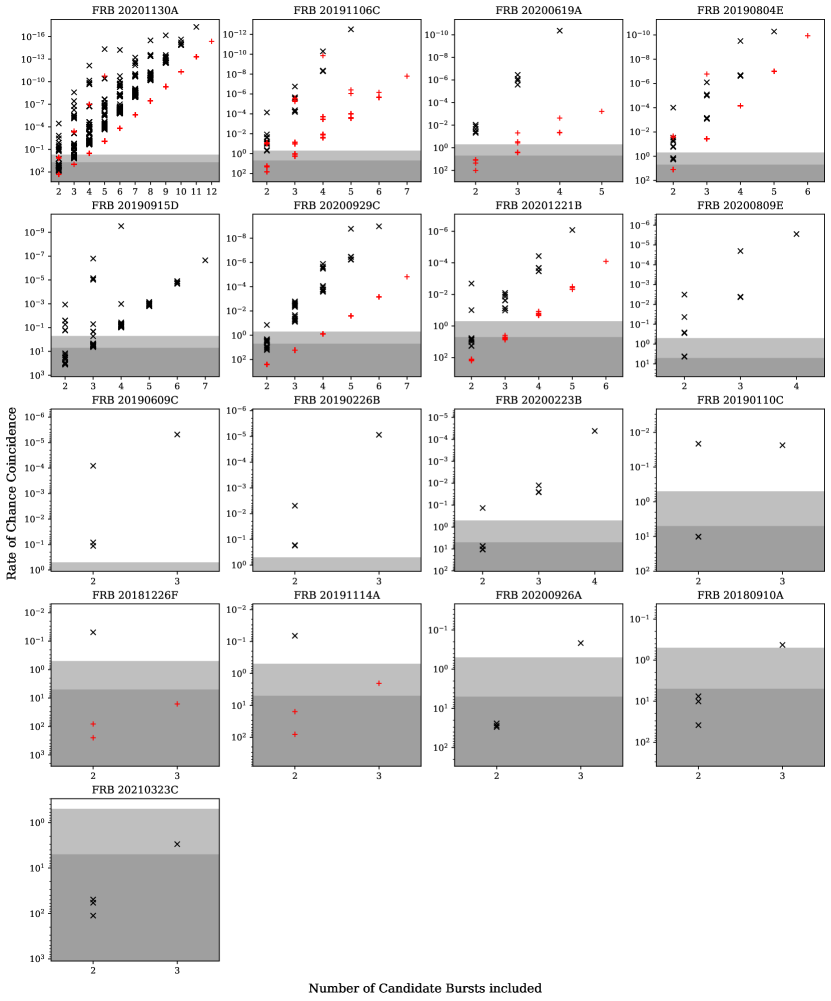
Figure 14: Contamination rate ($R_{\mathrm{cc}}$) of all combinations of bursts in clusters of 3+ events. Note that the vertical axes are inverted. The gray regions indicate $0.5\leq R_{\mathrm{cc}}<5$ (silver sample; lighter region) and $R_{\mathrm{cc}}\geq 5$ (darker region). Potential outlier events are marked by red pluses, all other events by black crosses (§2.2.2).

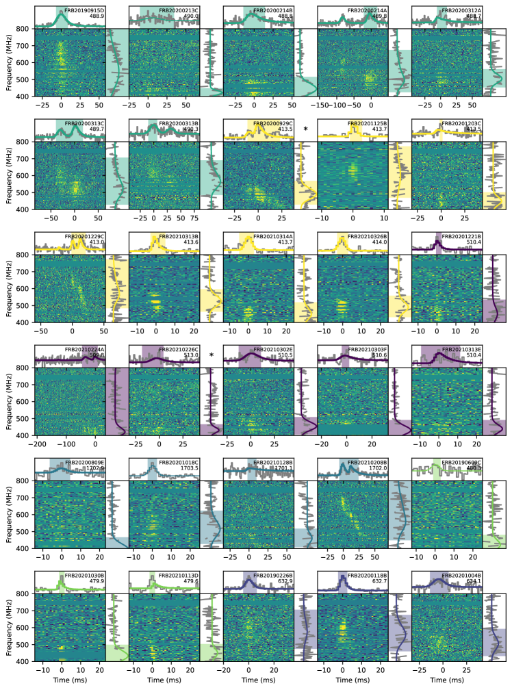
Figure 15: Continued from Figure 5.

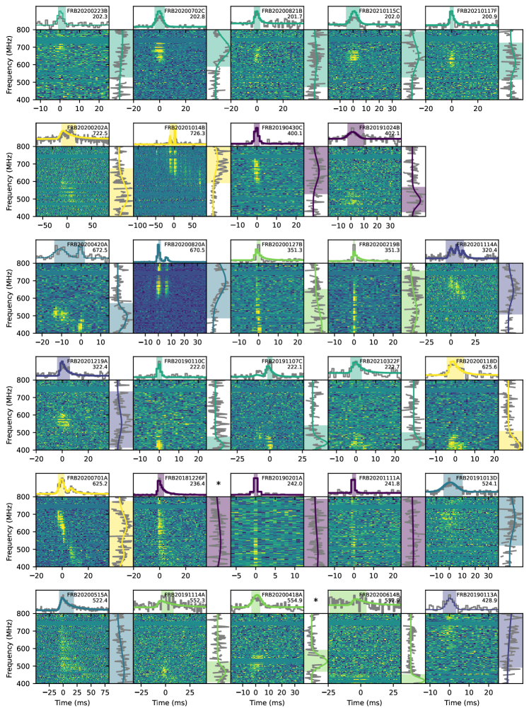
Figure 16: Continued from Figure 5.

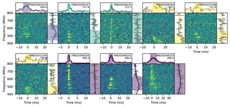
Figure 17: Continued from Figure 5.

As it is possible that a cluster contains unrelated bursts (e.g., from the tolerances of the clustering analysis being large; see §2.2.1), we calculate $R_{\mathrm{cc}}$ for each combination of events in a cluster and consider the minimum $R_{\mathrm{cc}}$ of all combinations (which should be the $R_{\mathrm{cc}}$ of all events in a cluster, if no event is an outlier). We inspect all combinations (see Fig. 14 in Appendix D) and flag those events that increase the $R_{\mathrm{cc}}$ by more than an order of magnitude as compared to the minimum $R_{\mathrm{cc}}$ of that cluster in one or more of the combinations (ten potential outliers in total in nine unique candidate clusters; these flagged events are marked with asterisks in Figs. 5, 15–17). However, we do not exclude from our sample those flagged events, as a mix of parameter uncertainties (sky positions from real-time detection S/Ns versus baseband data and a S/N-dependent DM uncertainty) could also lead to a “forked path” of $R_{\mathrm{cc}}$ as a function of included events, where one event leads to a systematically lower $R_{\mathrm{cc}}$ when combined with other events in the cluster (see Fig. 14 for examples). The outlier analysis would also reveal if two or more separate repeaters were grouped into one cluster, but we see no evidence for this.

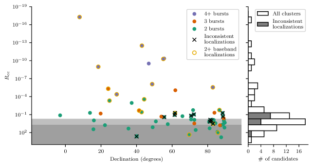
Figure 1: The panel on the left shows the minimum contamination rate ($R_{\mathrm{cc}}$) of all combinations of bursts in 65 clusters of events as a function of the average declination of the cluster. Note that the vertical axis is inverted. The gray regions indicate $0.5\leq R_{\mathrm{cc}}<5$ (“silver” sample; lighter region) and $R_{\mathrm{cc}}\geq 5$ (darker region), markers are color-coded by cluster size, and clusters with inconsistent localizations (which are then discarded) are indicated with a black cross. The panel on the right shows a histogram of the $R_{\mathrm{cc}}$. In general, clusters with more bursts and/or baseband localizations and clusters at lower declination have lower $R_{\mathrm{cc}}$.

3 Analysis & Results

The properties of 25 new repeating sources of FRBs are summarized in Table 1 and individual burst properties are collected in a machine-readable table in the same format as the first CHIME/FRB FRB catalog (CHIME/FRB Collaboration et al., 2021). A description of each field in the catalog is presented in Table LABEL:ta:catalog_descriptions in Appendix C. A sky distribution of repeating sources of FRBs is presented in Figure 2. Dedispersed dynamic spectra of the bursts, best-fit localization regions of each source without any baseband localization (see §3.1) and the exposure up to 2021 May 1 are publicly available.

Figure 3 shows the detection timeline of all repeating sources of FRBs discovered and detected (i.e., FRB 20171019A, originally discovered by ASKAP; Kumar et al., 2019) by CHIME/FRB up to 2021 May 1, including previously unpublished bursts from already published sources. Of the previously unpublished bursts from the known sources, we have measured their burst properties if their first detection with S/N $>$ 10 or 12 happens to be an unpublished burst for the analysis in §3.3. We use the detection S/N and times-of-arrival of these bursts for the analyses in §4.4 and §4.5. A machine-readable table of these bursts is available in the same format and at the same location as the table with bursts from the new sources.

Results on host galaxies to the new sources will be reported by Ibik et al. (in prep.), on associated persistent radio emission by Ibik et al. (in prep.) and on cross-correlation with galaxy catalogs by Rafiei-Ravandi et al. (in prep.).

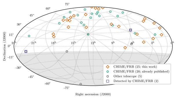
Figure 2: Sky distribution (Aitoff projection) of repeating sources of FRBs discovered by CHIME/FRB (orange open diamonds and green open circles; this work and CHIME/FRB Collaboration et al., 2019a, b; Fonseca et al., 2020; Bhardwaj et al., 2021a; Lanman et al., 2022), discovered by other telescopes (gray open circles; Spitler et al., 2016; Kumar et al., 2019; Luo et al., 2020; Kumar et al., 2021; Niu et al., 2022) and detected by CHIME/FRB (purple open squares; Josephy et al., 2019; Patel & CHIME/FRB Collaboration, 2019). $\delta<-11^{\circ}$ is outside of CHIME/FRB’s field-of-view and shaded light gray. The gray solid lines in the background show the plane of the Galaxy ($b=0^{\circ}$) as well as lines of constant Galactic longitude $0^{\circ}$ to $360^{\circ}$ in steps of $30^{\circ}$.

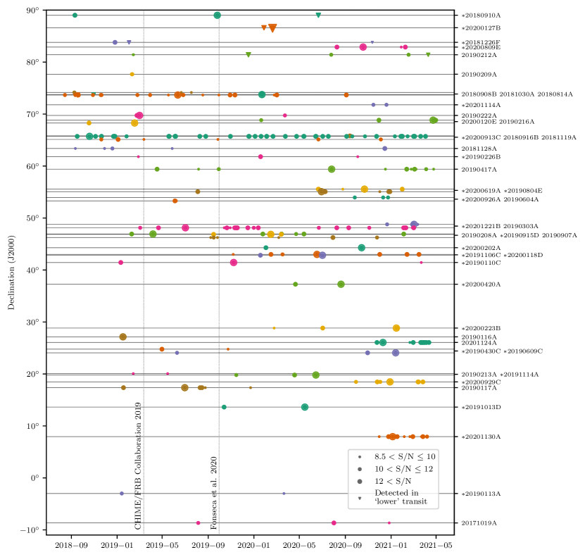
Figure 3: Detection timeline for 46 repeating sources of FRBs (45 discovered by CHIME/FRB and FRB 20171019A; Kumar et al., 2019) from the start of CHIME/FRB operations to 2021 May 1. Different sources have different colors, detections in the “lower” transit are indicated by a downward-facing triangle and repeater discovery dates (when the second burst above a completeness threshold, here S/N $>$ 12, was detected — not the case for all sources; see §4.5) are highlighted with an extra circle or triangle. Source names are listed on the right-hand ordinate axis, with an asterisk in front of the names of the 25 newly discovered repeaters. To aid readability, source names have sometimes been grouped in a row in order of descending declination. Dotted vertical lines mark the cutoff dates for CHIME/FRB Collaboration et al. (2019b) and Fonseca et al. (2020).

Table 1: Properties of 25 New Repeating Sources of FRBs, Ordered by Increasing $R_{\mathrm{cc}}$ (Our “Gold” Sample)

FRB Sourcea	$R_{\mathrm{cc}}$	$\alpha^{b}$	$\delta^{b}$	$l^{c}$	$b^{c}$	DMd	DM${}_{\rm NE2001}^{e}$	DM${}_{\rm YMW16}^{e}$	Nbursts	Exposuref	Completenessg	Burst rateh
		(J2000)	(J2000)	(deg)	(deg)	(pc cm-3)	(pc cm-3)	(pc cm-3)		(hr, upper / lower)	(Jy ms)	(hr-1)
20201130A	$5.3\times 10^{-18}$	64.39(1)	7.94(1)	$185.4$	$-29.0$	287.984(7)	56	69	12	$15\pm 11$	$10.4$	2.34${}_{-2.01}^{+2.28}$
20191106Ci	$3.1\times 10^{-13}$	199.58(1)	43.002(9)	$105.7$	$73.2$	333.40(2)	25	21	7	$66\pm 3$	$1.9$	$(2.54_{-1.35}^{+2.23})\times 10^{-2}$
20200619A	$4.3\times 10^{-11}$	272.6(1)	55.56(6)	$84.0$	$27.8$	439.772(4)	51	45	5	$110\pm 6$	$2.5$	$(1.3_{-0.9}^{+1.7})\times 10^{-2}$
20190804E	$5.2\times 10^{-11}$	261.34(2)	55.069(8)	$82.9$	$34.1$	363.68(1)	43	37	6	$94\pm 4$	$1.9$	$(1.52_{-0.86}^{+1.49})\times 10^{-2}$
20190915D	$3\times 10^{-10}$	11.78(3)	46.86(2)	$122.2$	$-16.0$	488.69(2)	89	88	7	$92\pm 1$	$11.3$	$(2.56_{-1.36}^{+2.25})\times 10^{-1}$
20200929Ci	$10^{-9}$	17.04(2)	18.47(1)	$128.5$	$-44.2$	413.659(4)	38	29	7	$56\pm 2$	$5.5$	$(1.45_{-0.77}^{+1.27})\times 10^{-1}$
20201221Bi	$8.3\times 10^{-7}$	124.20(3)	48.78(2)	$170.5$	$33.8$	510.42(5)	51	46	6	$90\pm 2$	$3.4$	$(3.78_{-2.13}^{+3.68})\times 10^{-2}$
20200809E	$2.8\times 10^{-6}$	20.0(1)	82.89(2)	$123.9$	$20.1$	1703.48(1)	74	83	4	$510\pm 2$ / $410\pm 26$	2.5 / 6.1	$(2.81_{-1.85}^{+3.61})\times 10^{-3}$
20190609C	$4.8\times 10^{-6}$	73.32(1)	24.068(6)	$177.4$	$-12.4$	479.602(9)	113	154	3	$72\pm 0$	$2.1$	$(7.3_{-6.0}^{+15.7})\times 10^{-3}$
20190226Bj	$8.7\times 10^{-6}$	$273.62_{-0.34}^{+0.17}$	$61.67_{-0.14}^{+0.41}$	$90.9$	$28.0$	632.597(9)	51	45	3	$85\pm 52$	$1.1$	$(3.65_{-3.47}^{+6.20})\times 10^{-3}$
		$270.25_{-0.24}^{+0.38}$	$61.93_{-0.41}^{+0.15}$	$91.1$	$29.6$		48	43
20200223Bi	$4.1\times 10^{-5}$	8.265(8)	28.831(7)	$118.1$	$-33.9$	202.268(7)	46	37	5	$52\pm 2$	$7.6$	$(1.44_{-0.95}^{+1.86})\times 10^{-1}$
20200202A	$0.00028$	25.93(2)	44.290(7)	$132.7$	$-17.6$	722.37(7)	83	84	2	$62\pm 5$	$6.1$	$(6.53_{-4.78}^{+10.40})\times 10^{-2}$
20190430C	$0.00047$	277.210(9)	24.770(9)	$53.1$	$15.7$	400.57(1)	100	84	2	$29\pm 7$	$11.5$	$(2.36_{-2.02}^{+5.11})\times 10^{-1}$
20200420A	$0.0011$	$7.57_{-0.02}^{+0.04}$	$37.26_{-0.06}^{+0.04}$	$118.3$	$-25.4$	671.5(4)	58	50	2	$55\pm 29$	$0.7$	$(9.58_{-10.40}^{+36.20})\times 10^{-4}$
20200127B	$0.017$	119.2(1)	86.609(8)	$126.6$	$28.0$	351.3(4)	54	51	2	$154\pm 13$ / $951\pm 18$	3.7 / 5.3	$<1.05\times 10^{-2}$
20201114A	$0.018$	221.59(8)	71.79(3)	$111.2$	$42.6$	322.23(1)	38	31	2	$135\pm 27$ / $83\pm 17$	6.8 / 66.3	$(2.33_{-1.98}^{+5.03})\times 10^{-2}$
20190110C	$0.021$	249.33(1)	41.445(9)	$65.6$	$42.1$	221.92(1)	37	30	3	$45\pm 11$	$1.2$	$(8_{-6}^{+13})\times 10^{-3}$
20200118D	$0.038$	106.91(1)	42.837(9)	$174.4$	$20.9$	625.57(3)	77	92	2	$72\pm 5$	$1.2$	$(3.3_{-2.7}^{+7.1})\times 10^{-3}$
20181226F	$0.049$	$95.87_{-0.31}^{+0.23}$	$83.80_{-0.16}^{+0.47}$	$129.8$	$26.2$	241.887(3)	58	56	3	$394\pm 192$ / $376\pm 215$	4.8 / 10.6	$(2.37_{-2.53}^{+8.96})\times 10^{-3}$
20191013D	$0.051$	40.42(2)	13.63(3)	$159.7$	$-41.3$	523.57(3)	43	36	2	$67\pm 1$	$8.9$	$(7.09_{-5.83}^{+15.20})\times 10^{-2}$
20191114A	$0.066$	273.57(3)	19.80(4)	$47.0$	$16.8$	552.47(6)	98	80	3	$61\pm 5$	$2.1$	$(1.36_{-0.99}^{+2.16})\times 10^{-2}$
20190113Aj	$0.13$	$108.26_{-0.26}^{+0.29}$	$-2.98_{-0.52}^{+0.51}$	$218.1$	$3.4$	428.90(1)	178	251	2	$40\pm 25$	$5.0$	$(4.97_{-5.13}^{+11.10})\times 10^{-2}$
		$106.56_{-0.80}^{+0.78}$	$-3.01_{-0.56}^{+0.54}$	$217.3$	$1.9$		187	275
20200913C	$0.18$	269.03(6)	65.80(3)	$95.5$	$30.2$	576.880(3)	48	43	2	$156\pm 3$	$1.8$	$(2.85_{-2.34}^{+6.12})\times 10^{-3}$
20200926A	$0.22$	$283.28_{-0.20}^{+0.18}$	$53.95_{-0.31}^{+0.30}$	$83.7$	$21.4$	758.44(5)	64	59	3	$67\pm 43$	$0.5$	$(1.58_{-1.53}^{+2.70})\times 10^{-3}$
20180910A	$0.43$	354.8(9)	89.01(1)	$122.6$	$26.2$	684.408(1)	56	55	3	$3913\pm 270$ / $4335\pm 26$	19.1 / 30.7	$(3.83_{-3.16}^{+8.23})\times 10^{-3}$

^a Here we employ the TNS naming convention, see https://www.wis-tns.org/astronotes/astronote/2020-70.
^b Positions were determined from baseband data (symmetric uncertainties) where available and from per-burst S/N data otherwise (asymmetric uncertainties; see §3.1), and uncertainties are at 90% confidence.
^c Galactic longitude and latitude for the best position.
^d Inverse-variance-weighted average DM, and the uncertainty in the calculation of that average. In cases where the DM was fixed in the fitburst fit, we set the DM uncertainty to 0.5 pc cm^-3 for the calculation of the average. For candidates with large DM variation from burst to burst, this average and its uncertainty may not necessarily be representative and we advise looking at the individual burst DMs using generous DM ranges when conducting follow-up searches of these candidates.
^e Maximum model prediction along this line-of-sight for the NE2001 (Cordes & Lazio, 2002) and YMW16 (Yao et al., 2017) Galactic electron density distribution models. Neither model accounts for DM contributions from the Galactic halo, which contributes no more than 111 pc cm^-3 (Cook et al., 2023).
^f For sources observed twice a day, the second entry corresponds to the less sensitive lower transit. The uncertainties in the total exposure for the upper and lower transits of each source are dominated by the corresponding source declination uncertainties since the widths of the synthesized beams vary significantly with declination.
^g Fluence completeness limits are given at the 90% confidence level. For sources observed twice a day, the second entry corresponds to the less sensitive lower transit.
^h Adjusted to a 5 Jy ms fluence threshold, assuming a $-1.5$ power-law energy index.
ⁱ The best-known sky position of this source falls in between the FWHMs at 600 MHz of the synthesized beams. We report the exposure at the beam centre of the nearest beam and have scaled the fluence completeness threshold accordingly.
^j Two equally likely “islands” in the localization 90% confidence region.

3.1 Localization

For the purposes of clustering events to obtain repeater candidates, we use the positions from the real-time detection pipeline (“header” localization), which are based solely on the per-beam S/N values. This localization method has been used for past CHIME/FRB publications; most recently CHIME/FRB Collaboration et al. (2021). For an in-depth description of this localization methodology, see CHIME/FRB Collaboration et al. (2019b). Briefly, the method is a grid-search $\chi^{2}$ minimization, where observed ratios among per-beam S/N values are compared to predictions from the CHIME/FRB beam model, over a grid of possible sky locations. The method can be applied to multiple bursts from the same source by summing the $\chi^{2}$ values for each data set. As the best-fit sky position, we construct a 90% confidence region. For most sources, this forms one “island”, but for a few sources (FRB 20190226B and FRB 20190113A) two islands are equally likely, and we present two best-fit localizations in Table 1.

For those bursts for which baseband data were saved to disk, we run the baseband pipeline detailed by Michilli et al. (2021) to generate a sky-localization. This pipeline works in two main stages. First, a crude grid of tied-array beams is formed to determine whether the burst occurred in a sidelobe, and to obtain an initial position estimate. Next, a tightly-packed grid of beams is formed around the initial position to get a refined best-estimate position. In $\sim$20% of cases, the baseband pipeline does not converge, due to a combination of low S/N, dedispersion artefacts and other reasons. Work to debug these issues is underway, and we defer those baseband localizations to future work. We do still include the events in our analysis, but use their positions from the real-time detection pipeline.

When one or more baseband localizations are available, a combined position is calculated using the inverse-variance weighted mean. The uncertainties on the combined sky positions are likely overestimated, as the systematic uncertainties are accounted for in each individual error bar (Michilli et al., 2021). We defer a more precise treatment of the combined systematics to future work. When no baseband localization for a source is available, a final best sky position for each source is calculated from combining header localizations as was done by Fonseca et al. (2020).

When labelling a collection of events as a candidate repeater, localization consistency is crucial to check. The nature of this check depends on the available data. For candidates with multiple baseband triggers, we verify the positions are consistent such that a weighted average yields no outliers. We also ensure any given baseband position is consistent with the uncertainty region derived from the header data alone, and we verify that each position is localized to the correct lobe of the formed beams and not a sidelobe. Baseband positions that are contained within the 90% confidence region are considered fully consistent, those in close proximity (within a few arcminutes) are considered marginal, and those several arcminutes to a few degrees away are considered outliers. For all repeater candidates, a successful joint-fit header localization is the baseline requirement. This test fails for seven clusters in the “gold” and four clusters in the “silver” sample; see §2.2.2 and Fig. 1, and those clusters are discarded. Conceptually, the joint fit is similar to taking the intersection of the uncertainty regions of individual bursts. Individual uncertainty regions reflect the instantaneous sensitivity of the beams that resulted in the detection, as well as those that did not. A merged localization with (near-)zero sky area is indicative of bursts that do not originate from the same sky location. We take all combinations of events from a cluster and check the merged localizations. If just one event led to the (near-)zero sky area, we discard that event. If all events in a cluster are inconsistent with each other, we discard the full cluster.

Figure 4 shows four source localizations that represent four possible ways in which the combined header and (combined) baseband positions can converge to the true sky position of a source. In the example of FRB 20190430C (top left), multiple header localizations do not greatly reduce the allowed phase space, and the baseband positions land on the main island. In the example of FRB 20190110C (top right), the central region is ruled out by combining multiple header localizations, and this is confirmed by the positions derived from baseband data. In the examples of FRBs 20191106C (bottom left) and 20191105B (bottom right), combining multiple header localizations reduces the allowed phase space in the North-South/declination direction. The baseband positions fall on the mainlobe island for the former source, but on a sidelobe island for the latter source.

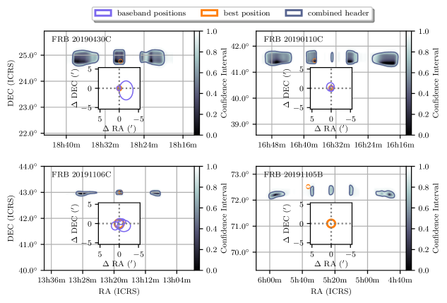
Figure 4: Four representative examples of combined localization patterns, as a function of right ascension (RA) and declination (DEC). The gray shaded area shows the 90% confidence region of the combined header (real-time detection) localization with the best-known position overlaid in orange. The insets show a zoom-in around the combined baseband localization (orange) on top of the individual baseband localizations (purple) shown as well. The combined header localizations allow for multiple possible degenerate islands and the baseband localizations can break that degeneracy.

3.2 Burst and Source Properties

We characterize each new burst as in the first CHIME/FRB catalog (CHIME/FRB Collaboration et al., 2021). In summary, we employ a least-squares fitting algorithm that allows for multiple components and provides measurements of DM and scattering (for each burst) and times-of-arrival, widths and spectral properties (for each burst component). Width and scattering timescales can be robustly measured from CHIME/FRB intensity data for values larger than $100\,\mu$s. Additionally, we determine a bandwidth and duration from the burst dynamic spectrum dedispersed to the best-fit DM. Flux and fluence are determined from converting the measured intensities to physical quantities using daily observations of bright calibration sources with known flux densities. CHIME/FRB exposure and sensitivity are calculated based on metrics collected that included instrument uptime and monitoring of detection S/Ns of known pulsars. Finally, we determine a fluence detection threshold for each source to characterize our completeness. This is based on a Monte Carlo analysis that takes into account uncertainties in the sky position and the spectral properties of the source. Burst rates are calculated from the number of detections and exposure to a source. While approximately 19 FRBs in the sample show downward-drifting subbursts by eye, obtaining robust drift rate measurements is challenging due to low detection S/N. We defer such measurements to later work.

Figures 5, 15–17 show dynamic spectra for each burst of each source. As before, most repeater bursts show narrow bandwidths of typically 50–200 MHz, with some sources showing bursts with clear cases of downward-drifting subbursts (FRBs 20190804E, 20190915D, 20200929C, 20200809E, 20201014B, 20200420A, 20201114A and 20200118D) of a few to tens of MHz ms^-1. Interestingly, FRBs 20200127B and 20181226F at modest extragalactic DMs ($\lesssim 300$ pc cm^-3) show larger bandwidths and narrower widths than is commonly observed for repeaters, reminiscent of bursts from other nearby sources FRBs 20181030A (Bhardwaj et al., 2021b) and 20200120E (Bhardwaj et al., 2021a). Some notable bursts: FRB 20210327F of source FRB 20201130A shows two resolved components spaced by about 300 MHz and a few seconds, FRBs 20200214A, 20200313C and 20200313B of source FRB 20190915D show two subbursts separated by $\sim$60, 30 and 30 ms, respectively, and FRB 20201014B of source FRB 20200202A shows at least seven subbursts with a spacing that shows a hint of possible periodicity, which is not statistically significant.

A preliminary long-term periodicity search with an algorithm that uses a Pearson’s $\chi^{2}$ test (e.g., CHIME/FRB Collaboration et al., 2020b) for all sources yielded no detections, which is not surprising as the largest number of bursts detected for a single source in this sample is only 12.

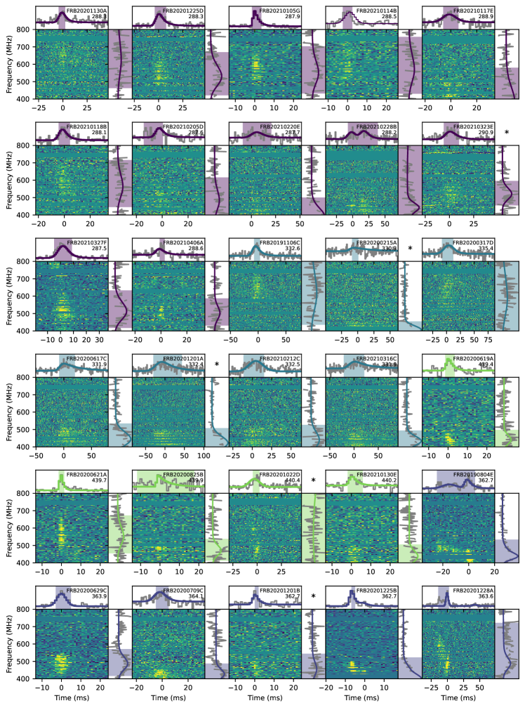
Figure 5: Dynamic spectra (“waterfall plots”), frequency-averaged time series and time-averaged spectra for all sources, ordered from high to low $R_{\mathrm{cc}}$. Bursts from the same source are grouped by the same color. In the upper right-hand corner of each panel are the the TNS names and DM values in units of pc cm^-3. The model fits for which scattering was determined to be insignificant are over-plotted in the time series and spectra with thin blue lines, whereas the fits for which scattering was determined to be significant are over-plotted in the time series and spectra with thick blue lines. The colored shaded regions in the time series and frequency spectra span the respective full width at tenth of maximum (FWTM) burst widths and emission bandwidths. An asterisk in the top right corner of a panel indicates that the event is a potential outlier, based on how it changes the $R_{\mathrm{cc}}$ of the cluster it belongs to (see §2.2.2). Continued in Figs. 15–17.

3.3 Comparison Analysis

Whether repeating FRBs represent a distinct population of astrophysical objects from those that have not been seen to repeat remains an open question. It is possible that, in time, all FRB sources will eventually emit repeat bursts. However, wait times between bursts may be long. It is therefore worthwhile to investigate other possible differences between the repeating and apparently-nonrepeating classes of FRBs.

For this reason, CHIME/FRB Collaboration et al. (2021) reported on a statistical comparison of repeater and apparent nonrepeater burst properties. This study revealed significant differences in both burst width and bandwidth, as studied in much greater detail by Pleunis et al. (2021b). However, no other statistically significant differences in morphological properties (e.g., DM, scattering) were identified.

Here we repeat the statistical comparison first reported in CHIME/FRB Collaboration et al. (2021), now including the repeater sample reported on here, together with all other published CHIME/FRB-discovered repeaters (CHIME/FRB Collaboration et al., 2019a, b; Fonseca et al., 2020; Bhardwaj et al., 2021a; Lanman et al., 2022; Kumar et al., 2019). In this analysis, we compare all the same properties as for CHIME/FRB Collaboration et al. (2021), between the new, much larger sample of repeating FRB sources, and the Catalog 1 apparent nonrepeaters. We also compare the previously published CHIME/FRB repeater sample with the new repeater sample, to compare samples discovered with different total sky exposures. The more detailed study of Pleunis et al. (2021b) is beyond our scope, and also unlikely very informative as the differences in morphology and spectra clearly persist strongly (see §3.3.2 below).

As in the CHIME/FRB Collaboration et al. (2021) analysis, we apply the following constraints when defining our comparison samples:

• Events with bonsai (real-time detection pipeline) S/N $<$ 12 are rejected to mitigate completeness issues.

• Events with DM $<$ 1.5 max($\textrm{DM}_{\textrm{NE2001}}$, $\textrm{DM}_{\textrm{YMW16}}$) are rejected to avoid misidentifying rotating radio transients or radio pulsars as FRBs due to $\sim$50% errors from models used to estimate the Galactic DM.

• Events detected in sidelobes are rejected since our understanding of the shape of the primary beam at large zenith angles is poor, rendering event characterization challenging.

With these cuts, 155 events are rejected from the nonrepeaters sample, four sources are rejected from the previously published CHIME/FRB repeaters sample, and 18 sources are rejected from our new repeaters sample. The remaining events represent a total of 305 apparent nonrepeaters, 14 previously published CHIME/FRB repeaters, 26 new repeaters (22 from the repeater sample reported here and four from other CHIME/FRB-discovered repeaters not included in Catalog 1), for a total of 40 CHIME/FRB repeating sources.

Note that below, we also relax some of these constraints in order to probe sensitivity of source selection in our comparison analysis. One significant difference in this analysis compared to that reported by CHIME/FRB Collaboration et al. (2021) is that we no longer require the first-detected burst from a repeater to exceed the S/N cutoff, but rather that any of the detected bursts exceed the S/N cutoff. This is because our repeaters are now identified through a clustering algorithm that can find repeating sources whose first event is not very bright (i.e., we consider all events with S/N $>$ 8.5). In our analysis described next, we use the first repeating event from each repeating source discovered by CHIME/FRB that satisfies all the conditions listed above.

For distribution comparisons with uncensored data (i.e., those without upper or lower limits), we report both Anderson–Darling (AD) and Kolmogorov–Smirnov (KS) tests. A $p$-value of $<$ 0.01 indicates 99% confidence that two samples originate from different distributions. For censored data, we apply statistical survival tests that consider upper and lower limits because we lose information if we directly omit censored data. For properties that have upper limits (pulse width and scattering time), we use both the Peto & Peto test and the log-rank test, using R NADA package’s cendiff function (Helsel, 2005; Lopaka, 2020; R Core Team, 2020). For events with properties containing lower limits (fluence and flux), a right censored survival test is applied using R NADA package’s survdiff function (Lopaka, 2020; R Core Team, 2020; Harrington & Fleming, 1982).

3.3.1 New versus Previously Published CHIME/FRB Repeater Comparison

Here we compare properties of previously published and new CHIME/FRB repeaters to determine whether the sample discovered with longer total exposure time differs from that discovered sooner. For example, a sample discovered with longer exposure time might be expected to have a larger mean DM, since a longer exposure may provide more distant sources sufficient time to produce two detectable bursts.

We compare distributions of right ascension, declination, DM, eDM, bonsai S/N, fitburst S/N, boxcar width, bandwidth, fluence, flux, width, and scattering. Here, eDM is defined as the DM after subtracting the NE2001 expected maximum Galactic contribution towards the source. In all cases except flux, $p$-values are $>$ 0.01. However, we note that lower limits dominate in the fluxes in both the published sample and the new sample (all fluxes in the published sample are censored). Additionally, the fluxes of the new repeaters are more reliable due to better localizations while the fluxes of the previously published repeaters have more uncertainty. Thus, we cannot be confident of the difference in flux. We conclude that there is a lack of significant differences between the two samples’ properties. This may be due to insufficient difference in exposure time for samples of these sizes to yield a significant detection, or too few sources to permit any difference detection.

3.3.2 Repeater versus Apparent Nonrepeater Comparison

The $p$-value results of our statistical tests comparing repeaters and apparent nonrepeaters are shown in Table 2. For distributions of right ascension, declination, bonsai S/N, fitburst S/N, fluence, and flux, we find that the distributions for repeaters and nonrepeaters are consistent with having been drawn from the same population, as we did in our prior analysis. For burst width (both measured and box car) and spectral parameters, we continue to see a statistically significant distinction between distributions, consistent with that previously studied by Pleunis et al. (2021b), which will be further quantified in a future paper. Pleunis et al. (2021b) found $p$-value = $10^{-3}$ when comparing width between repeaters and nonrepeaters, and here, we find $p_{AD}=1.88\times 10^{-8}$ and $p_{KS}=3.73\times 10^{-5}$. For bandwidth, Pleunis et al. (2021b) observed $p$-value = $10^{-5}$, and we observe $p_{AD}=1.24\times 10^{-8}$ and $p_{KS}=5.35\times 10^{-8}$. Pleunis et al. (2021b) obtained $p$-value = $10^{-4}$ for boxcar width, and we get $p_{AD}=2.49\times 10^{-5}$ and $p_{KS}=6.20\times 10^{-5}$ in our analysis. Furthermore, with the new, larger sample of repeaters, we now detect a new potential difference in the two distributions, as detailed next.

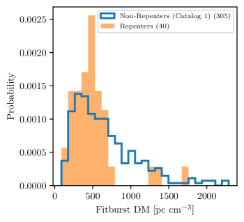
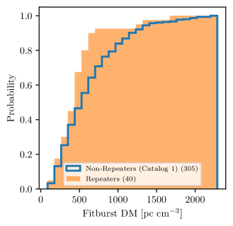
Figure 6: Normalized histogram (left) and cumulative distribution (right) of the DM of the 305 nonrepeating events from CHIME/FRB Collaboration et al. (2021, blue) and the complete sample of 40 CHIME/FRB-discovered repeating sources of FRBs (orange).

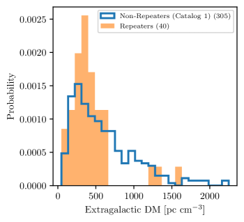
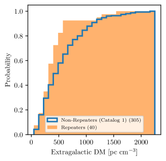
Figure 7: Normalized histogram (left) and cumulative distribution (right) of the eDM of the 305 nonrepeating events from CHIME/FRB Collaboration et al. (2021, blue) and the complete sample of 40 CHIME/FRB-discovered repeating sources of FRBs (orange).

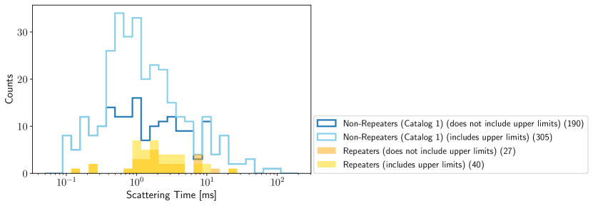
Figure 8: Histogram of the scattering times of the 305 nonrepeating events from CHIME/FRB Collaboration et al. (2021, light blue) and the minimum scattering times of the complete sample of 40 CHIME/FRB-discovered repeating sources of FRBs (light orange) on a log scale. Histograms of scattering times after discarding censored values are overplotted (dark blue for nonrepeaters and dark orange for repeaters).

DM Comparisons

Figure 6 compares the DM distribution of all one-off events in CHIME/FRB Collaboration et al. (2021) and the complete sample of CHIME/FRB-discovered repeating sources of FRBs. Our results suggest a significant difference in the DM distributions of repeaters and nonrepeaters. The AD and KS tests give $p_{\textrm{AD}}=0.0112$ and $p_{\textrm{KS}}=0.00618$, which suggest observed nonrepeaters and repeaters come from different distributions. The analogous analysis previously reported by CHIME/FRB Collaboration et al. (2021) using a smaller repeater sample detected no such difference. To investigate the putative difference further, we examined how the $p$-values change as we lower the S/N constraint to 11 and 10, in order to increase the sample sizes, though at the possible expense of completeness, but noting that the latter applies both to repeaters and nonrepeaters. When the S/N threshold is set to $>$ 11, $p_{\textrm{AD}}=0.00425$ and $p_{\textrm{KS}}=0.00324$. For S/N $>$ 10, $p_{\textrm{AD}}=0.00196$ and $p_{\textrm{KS}}=0.00278$. Thus, we see that the differences become more significant at lower S/N thresholds where the sample sizes increase, as expected for a significant difference. For lower S/N cuts, the difference in mean DMs between repeaters and nonrepeaters also increases. At S/N $>$ 12, repeaters have a mean DM of 500 $\pm$ 50 pc cm^-3 and nonrepeaters have a mean DM of 662 $\pm$ 24 pc cm^-3, with a difference of 162 $\pm$ 55 pc cm^-3 between repeaters and nonrepeaters. At S/N $>$ 11, repeaters have a mean DM of 493 $\pm$ 47 pc cm^-3 and nonrepeaters have a mean DM of 668 $\pm$ 22 pc cm^-3, resulting in a difference of 175 $\pm$ 52 pc cm^-3 (means differ with $>99\%$ confidence). At S/N $>$ 10, repeaters have a mean DM of 495 $\pm$ 45 pc cm^-3 and nonrepeaters have a mean DM of 692 $\pm$ 23 pc cm^-3, giving a difference of 197 $\pm$ 50 pc cm^-3 (means differ with $>99\%$ confidence).

This result is also observed in eDM distributions, as shown in Figure 7. With our nominal cuts on the sample, we see a possible difference in the underlying distributions, with $p_{\textrm{AD}}=0.0105$ and $p_{\textrm{KS}}=0.00416$. The difference becomes more significant with lower S/N constraints (for S/N $>$ 11, $p_{\textrm{AD}}=0.00464$ and $p_{\textrm{KS}}=0.00465$; for S/N $>$ 10, $p_{\textrm{AD}}=0.00188$ and $p_{\textrm{KS}}=0.00204$), again supporting the existence of a difference in DM distributions between repeaters and apparent nonrepeaters. As the S/N threshold is lowered, the difference in mean eDM increases as well. For S/N $>$ 12, repeaters have a mean eDM of 436 $\pm$ 49 pc cm^-3 and nonrepeaters have a mean eDM of 597 $\pm$ 24 pc cm^-3, with a difference of 161 $\pm$ 55 pc cm^-3 between repeaters and nonrepeaters. At S/N $>$ 11, repeaters have a mean eDM of 431 $\pm$ 46 pc cm^-3 and nonrepeaters have a mean eDM of 602 $\pm$ 22 pc cm^-3, with a difference of 171 $\pm$ 51 pc cm^-3 (means differ with $>99\%$ confidence). At S/N $>$ 10, repeaters have a mean eDM of 431 $\pm$ 44 pc cm^-3 and nonrepeaters have a mean eDM of 627 $\pm$ 23 pc cm^-3, giving a difference of 196 $\pm$ 50 pc cm^-3 (means differ with $>99\%$ confidence).

We thus conclude that with the larger sample of repeaters reported here, we detect a significant difference in DM distribution between repeaters and apparent nonrepeaters, with repeater DMs systematically lower than those of apparent nonrepeaters. This difference persists when we also include the “silver” sample with the “gold” sample (events with $R_{\mathrm{cc}}<5$) while keeping the same nominal cuts restrictions. The possible reasons for this difference are discussed below in §4.

Scattering Time Comparisons

Next, we look at the distributions of scattering times. As many of our scattering measurements are upper limits, we make use of statistical survival tests to consider differences in distributions. The Peto & Peto and log-rank tests for the repeater versus apparent nonrepeater data indicate similar underlying distributions, with $p=0.2$ and $p=0.09$, respectively. Since large scattering times may be due to confusion with multiple sub-bursts merging together, making it hard to identify each sub-burst individually, we also compare the lowest scattering time of each repeating source with the scattering time of apparent nonrepeaters (see Fig. 8). We find that the Peto & Peto test yields $p=0.1$, and the log-rank test yields $p=0.07$, respectively, which shows there is no significant difference in scattering time distributions in the present samples. Even as we increase the sample size by lowering the S/N threshold to 10, we observe no significant difference (i.e., $p>0.01$ for the log-rank and the Peto & Peto test). Using NADA’s cenfit function (Helsel, 2005; Harrington & Fleming, 1982; R Core Team, 2020; Lopaka, 2020), we find the Kaplan-Meier estimate mean, which considers upper limits, of the lowest scattering time of repeaters to be 2.32 $\pm$ 0.63 ms and that of nonrepeaters to be 3.22 $\pm$ 0.50 ms.

Table 2: Summary of Repeater vs Apparent nonrepeater Distribution Comparisons for Nominal Cutoff Criteria

Property	$p_{AD}^{a}$	$p_{KS}^{b}$
Right Ascension	0.322	0.492
Declination	0.827	0.914
DM	0.0112	0.00618
eDMc	0.0105	0.00416
bonsai S/N	0.262	0.405
fitburst S/N	0.691	0.855
Boxcar width	2.49$\times$ 10-5	6.20 $\times$ 10-5
Bandwidth	1.24 $\times$ 10-8	5.35$\times$ 10-8
Property	Peto & Peto	Log-Rank
Fluenced	0.409	0.217
Fluxd	0.339	0.997
Widthe	1.88 $\times$ $10^{-8}$	3.73 $\times$ $10^{-5}$
Scatteringe	0.222	0.0859
Lowest Scatteringe,f	0.140	0.0674

Notes.
^aAnderson-Darling probability of originating from same underlying population.
^bKolmogorov-Smirnov probability of originating from same underlying population.
^cExtragalactic DM.
^dIncorporates lower limits — see §3.3.
^eIncorporates upper limits — see §3.3.
^fUses only lowest scattering time per repeater.

3.4 Burst Rate Analysis

Here we compute burst repetition rates for all our repeaters, putting them into the broader context of FRB burst rates.

To compute repetition rates, we first determine the on-sky exposure for each of the sources from the start of the experiment, 2018 August 28, through to 2021 May 1. We follow the exposure determination techniques previously used by CHIME/FRB Collaboration et al. (2021). In summary, we generate an all-sky exposure map for the aforementioned interval by querying metrics which characterize the up-time and sensitivity of the CHIME/FRB system. These metrics are combined with the CHIME/FRB beam model, under the assumption that a sky location is detectable if it is within the FWHM region of a synthesized beam at 600 MHz. We query the resulting exposure map over a grid of positions within the 90% confidence localization region for each source. The mean and standard deviation of the exposure over the corresponding positional grids are provided in Table 1 and Table 3, for the “gold” and “silver” samples, respectively. The exposure increases with declination, with the uncertainties in the exposure dominated by the corresponding source declination uncertainties.

In the interval used for the exposure calculation, we detected a total of 128 bursts from the 25 confirmed and 14 candidate repeaters presented in this paper (i.e., bursts that were detected outside the FWHM at 600 MHz of a synthesized beam were excluded from the burst rate computation). While calculating the burst rate, we exclude five of these bursts which were detected when the system was not operating nominally. Additionally, for circumpolar sources ($\delta>+70^{\circ}$), we exclude bursts detected in the lower transit. Therefore, we only compute the burst rate in the upper transit for all sources. This choice is motivated by the sensitivity of the primary beam being greater in the upper transit, which can provide a stronger constraint on the source activity. The sensitivity to each source also varies based on the synthesised beam response. This variation is accounted for in the 90% confidence completeness thresholds reported in Tables 1 and 3. To facilitate comparison across repeaters, we scale all burst rates to a fluence threshold of 5 Jy ms, i.e., the average sensitivity of the CHIME/FRB system (Josephy et al., 2021). The scaling involves the assumption of a power-law index of $-1.5$ for the cumulative burst energy distribution of each source. We set the index to be $-1.5$ to be consistent with the repetition rate analyses presented by CHIME/FRB Collaboration et al. (2019b) and Fonseca et al. (2020). The scaled repetition rates are plotted in Figure 9.

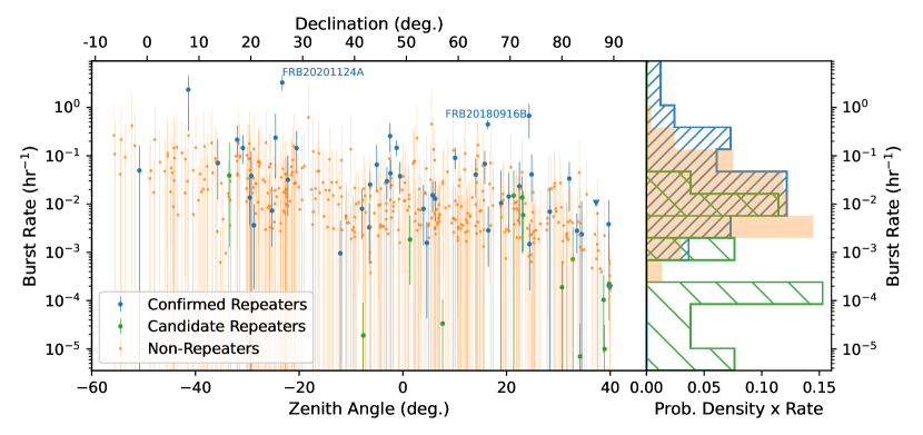
Figure 9: Burst rates of previously published and new repeaters, candidate repeaters (the “silver” sample) and Catalog 1 nonrepeaters as a function of zenith angle (bottom abscissa axis) and declination (top abscissa axis). For each source, the uncertainty on the rate is the quadrature sum of the 90% Poisson uncertainty and the uncertainty in the source exposure (see Tables 1 and 3). Histograms of the rate estimates for each class of sources are plotted in the right panel.

We also update the rate estimates for 19 previously published CHIME/FRB repeaters (CHIME/FRB Collaboration et al., 2019a, b; Fonseca et al., 2020; Lanman et al., 2022) by computing the exposure up to 2021 May 1 using the corresponding source localization regions (see Table 4 in Appendix B). For 13 of these sources, we use unpublished baseband localization regions (Michilli et al., in prep.). The localization regions published in the discovery papers are used for the rest of the sample. A total of 210 bursts (including unpublished detections) were observed in the upper transits of these sources, of which we exclude 15 bursts as they were detected in low-sensitivity periods. We scale the repetition rates to a threshold of 5 Jy ms, using the completeness thresholds reported in the discovery papers. To allow for comparison of the CHIME/FRB repeaters with the nonrepeaters, we also estimate burst rates for Catalog 1 one-off sources based on the detection of one burst from each source. Although CHIME/FRB Collaboration et al. (2021) report the detection of 474 such sources, we exclude 63 of them because of their detection in low-sensitivity periods or in the lower transit. Another 14 sources are excluded as they are found to be repeat bursts from the sources presented in this work. The rates for the remaining sources are estimated using the header localization regions and completeness thresholds reported by CHIME/FRB Collaboration et al. (2021), and are plotted in Figure 9.

Next we investigate whether the burst rates for the repeating sources are correlated with other properties, namely, extragalactic DM, intrinsic width, bandwidth, fluence and scattering. We perform this analysis with the confirmed and candidate repeaters presented in this work as well as the 19 previously published repeaters. For these 19 repeating sources, we use the burst properties reported in their discovery papers. Additionally, we determine properties of the unpublished detections from these sources using the techniques described in Section 3.2.

While testing for potential correlations, here we define eDM for a source as the mean extragalactic DM estimated using the NE2001 and YMW16 models. The source width is assumed to be the average of the intrinsic widths for all repeat bursts. If a repeat burst comprises of sub-bursts, we average the widths for the individual sub-bursts before using them to calculate the mean width for the source. We obtain the error on the mean width for each source as the quadrature sum of the uncertainties in the width measurements of the repeat bursts. We obtain mean bandwidths and fluences for each source and the corresponding errors in a similar manner. As for scattering, we adopt the strongest constraint among all repeat bursts as the scattering time for each source. This assumes that scattering structures along the line of sight to these sources do not change significantly in the interval between detections (but see Ocker et al., 2023). Due to the finite time resolution of the CHIME/FRB system, some width and scattering time measurements are upper limits. In such cases, we assume the 95% confidence upper limit to be the measured value.

While checking for a correlation of the repetition rate with these properties, we account for the errors in the measurements by performing 10,000 simulation runs. In each run, we sample a possible value of the burst rate and also of the property in consideration (say, the width) for each of the repeaters. For each repeater, we sample these values from a Gaussian distribution with a standard deviation equal to the 1$\sigma$ error on the burst rate and width. In each iteration, we check for a correlation using the Spearman’s rank-correlation test. We then obtain the median of the $p$-value for the test over all 10,000 iterations. The burst rates and other properties along with the associated median $p$-values are shown in Figure 10.

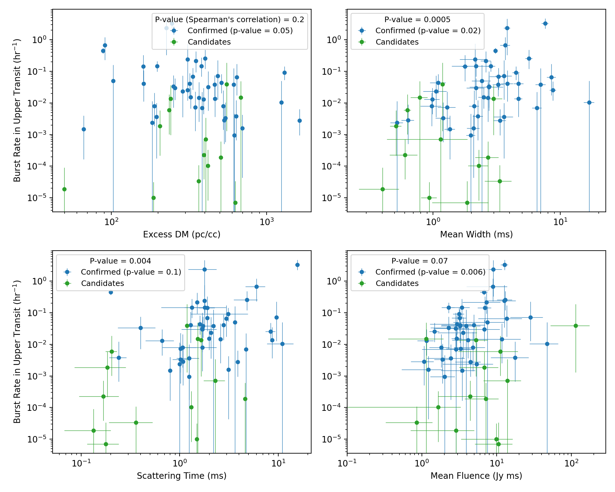
Figure 10: Burst rates of previously published and new repeaters (blue) and candidate repeaters (the “silver” sample; green) as a function of eDM (top left), mean width (top right), scattering time (bottom left) and mean fluence (bottom right). The title of the legend in each panel indicates the associated $p$-value for the Spearman rank-order correlation (confirmed and candidate repeaters; blue and green), with the null-hypothesis being that the plotted quantities are uncorrelated. The $p$-value for the test conducted only using the sample of confirmed repeaters (blue) is indicated in brackets. The errors represent the 90% confidence interval for the plotted quantities.

4 Discussion

4.1 Completeness of Repeater Identification

We believe that our repeater identification is complete for sources with properties similar to previously discovered repeaters (e.g., no extreme DM evolution). Next we discuss ways in which our $R_{\mathrm{cc}}$ calculation could be made more robust and sensitive in the future.

The clustering analysis (§2.2.1) at the root of the repeater search presented here has used large tolerances in sky position and DM, $\sigma_{\alpha}=2.2\arcdeg/\cos(\delta)$, $\sigma_{\delta}=0.5\arcdeg$ and $\sigma_{\mathrm{DM}}=13$ pc cm^-3, that reflect uncertainties in the CHIME/FRB detection pipeline. It successfully constructs clusters of repeater detections in the main lobes and first sidelobes of the beams, but it will miss repeat bursts in the far sidelobes of the telescope, if they are detectable (this depends on the luminosity function of the repeaters, see also Lin et al. in prep.). The algorithm groups together events with $\Delta$DM $\lesssim 13$ pc cm^-3, which makes it sensitive to mild putative DM evolution of repeating sources as well as to a range of DM measurement errors in the real-time detection pipeline. We allow for this range because in cases of downward-drifting subbursts, the DM can be overestimated by the S/N-optimizing detection pipeline as subbursts get superimposed for greater S/N (Hessels et al., 2019). Sources with DM evolution $\gtrsim 13$ pc cm^-3 would have been missed, but this level of DM evolution has not been observed in any source of FRBs.

The $R_{\text{cc}}$ calculation is limited by a few observational realities. The probability that we detect an FRB event in some volume $\Delta\alpha\Delta\delta\Delta$DM is a function of CHIME/FRB’s exposure and selection function (§2.2.2). This is therefore not trivial to calculate. Instead, we empirically estimate it using a normalized histogram of our entire FRB sample, including only one burst from each known repeater. This means that the data set that is used to construct the null case for the $R_{\mathrm{cc}}$ calculation is contaminated by repeating sources. Ultimately, this produces conservative $R_{\text{cc}}$ estimates, but an improved method would use an uncontaminated null data set or account for the contamination in some way. We control for the problem of multiple hypotheses testing by multiplying by $N$, the total number of FRBs in this sample. This a common correction for the look-elsewhere effect, and it has been shown to be conservative (Goeman & Solari, 2014).

Another factor that we do not account for is our pipeline-imposed increase in sensitivity for repeaters. As soon as an FRB candidate is detected we add it to a database of known sources. The S/N threshold for saving baseband data for any candidate is 12, but that threshold is lowered to 10 for events coincident with a known FRB source in the database. In principle, this should be accounted for in the empirical estimation of $p_{\{\alpha,\delta,\mathrm{DM}\}}$ but is non-trivial and will be the subject of future work.

The time between detections is also not accounted for in our $R_{\mathrm{cc}}$ calculation. Intuitively, FRBs with similar DMs and spatially coincident localizations that are detected in rapid succession (e.g., within a single CHIME/FRB transit) may seem more likely to be repeaters than those detected years apart. However, how to include this timing is not clear, particularly because we do not know the general temporal behavior of repeaters. More detailed quantitative characterizations of the waiting time distributions and other temporal properties of the repeater population could be helpful in this regard.

Future improvements to the $R_{\mathrm{cc}}$ framework could also allow for priors on additional parameters, such as the burst duration and bandwidths, which have been shown to be different for repeater bursts and one-off events (Pleunis et al., 2021b), or the scattering properties, when we understand better what variability can exist (see, e.g., Ocker et al., 2023). Regardless, CHIME/FRB aims to provide sky positions with subarcminute precision for many future FRBs through its “Outriggers” upgrade (Leung et al., 2021; Cassanelli et al., 2022), which will make identifying true repeaters among the sample easier in the future.

4.2 Comparison of New and Previously Known Repeater Samples

As stated in §3.3.1, we conclude that there is no significant difference between new and previously published CHIME/FRB repeater samples. All $p$-values are $>0.01$ except flux, which has a log-rank test $p$-value $<0.01$ but has large uncertainty due to the presence of many censored values. We might expect to detect more repeaters in this new sample at lower declination where CHIME/FRB’s sensitivity is lower, since more observation time has passed, but no difference in the declination distributions is observed. Similarly, due to longer total exposure, we might expect to see a difference in the DM distributions between previously published and new samples of repeaters since there is more opportunity to detect more distant repeaters, but no difference is observed.

This lack of any apparent difference could indicate no difference in the two samples’ properties, insufficient difference in exposure time for samples of these sizes to yield a significant detection, or too few sources to permit detection of any differences. Alternatively, the lack of an apparent difference between the new and previously published repeaters could be a result of FRBs having finite lifetimes, since the active lifetime of an FRB could end before a burst is detected. Or, new repeating sources (cf. FRBs 20201124A and 20220912) could “turn on” at all declinations and DMs at a rate comparable to the increase in discovery of sources at high DM and low declination with increased total exposure. The two competing rates could mask the expected increase in detections of more distant sources over time, especially when the total number of sources is still relatively low.

4.3 Comparison of Apparent Nonrepeating and Repeating Sources

As discussed in §3.3.2 and shown in Table 2, the AD and KS tests indicate that the DM and extragalactic DM (eDM) distributions of the full repeaters sample and Catalog 1 apparent nonrepeaters (meeting the criteria specified in §3.3.2) are seemingly inconsistent with arising from the same population. This inconsistency increases as we lower the S/N threshold. A likely explanation for the latter observation is that the sample size increases as we lower the S/N threshold, making any real differences more significant. If so, the difference in DM distribution between repeaters and apparent nonrepeaters is very significant. Such a difference could in principle indicate new, important support for the two source classes being of physically different origins. A difference in DM distribution could indicate a difference in one or more of (i) distribution in redshift space, (ii) host galaxy type, or (iii) local environment. However, none of these is necessary to explain the effect. Gardenier et al. (2021) showed that the detection of nonrepeaters and repeaters is inherently subject to different observational selection effects. If repeaters and nonrepeaters originate from the same population, we would observe a difference in DM distributions because a second bright burst required for a source to be identified as a repeater is more challenging to detect at higher DM, if the luminosity function universally declines at higher luminosity. Detailed population modelling will be required to determine whether the degree of the difference reported here can be explained by this simple bias assertion alone under reasonable assumptions of luminosity function, or whether one can conclude there is a genuine difference in source classes.

We do not observe a difference in scattering time distributions when we compare the first detected burst per source after the cuts stated in §3.3.2, nor do we observe a difference between the two distributions when we compare the lowest scattering time of each repeating source with nonrepeaters. We note that it is possible for scattering-time measurements to be biased by broad pulse widths and complex morphology. Since repeater bursts have been shown to have longer duration and more complex morphology (Pleunis et al., 2021b), we might expect a bias in which repeater bursts have longer scattering times compared to nonrepeaters. Yet, we observe repeaters to have comparable or even possibly lower scattering times both when we compare the first burst that passes the criteria in §3.3.2 (repeaters: 2.57 $\pm$ 0.77 ms; nonrepeaters: 3.22 $\pm$ 0.50 ms) and when we compare the minimum scattering time of each source (repeaters: 2.32 $\pm$ 0.63; nonrepeaters: 3.22 $\pm$ 0.50 ms). On the other hand, if there were a strong DM/scattering correlation, then repeaters having a lower mean DM and eDM than apparent nonrepeaters, as we observe, would suggest they should also have lower scattering times. However, strong DM/scattering correlations have not been seen in the FRB population (e.g., Chawla et al., 2022). Detailed population studies, preferably on burst properties measured using voltage data, for which the time resolution is higher, hence scattering may be more easily measured, will be needed to properly search our larger sample for such a correlation.

4.4 Burst Rates

Here we discuss the burst rate analysis shown in §3.4, where we found burst rates for all new (both “gold” and “silver” samples) and previously published CHIME/FRB repeaters, as well as for Catalog 1 nonrepeating sources (see Fig. 9).

First, we note that the estimated rates might not be equal to the true repetition rates of these sources because of two assumptions made in this analysis. First, assuming a power-law index of $-1.5$ for scaling the burst rates to a common fluence threshold will introduce rate errors of varying magnitudes for different sources. This is because the measured index for known repeaters varies widely, ranging from $-0.7$ to $-3.6$ (Law et al., 2017; Lanman et al., 2022). Second, some of the bursts in our sample could have been detected in the sidelobes of the synthesized beams. As the exposure map does not include exposure in the sidelobes, the true repetition rate for some sources could be lower than is reported here. However, as both these assumptions affect the estimated rates across all sources in a stochastic manner, they are unlikely to affect the conclusions of a rate comparison between the repeating and non-repeating populations and among the repeating sources.

Among the repeating sources, we find that the candidate repeaters have, on average, lower repetition rates as only two bursts have been detected from most of these sources. We also find that the burst rate is, on average, lower for high-declination sources. This is because the increased exposure at high declinations allows us to detect repeating FRBs with low repetition rates and place stricter constraints on the rates for the one-off sources. While some active repeating sources, such as FRB 20201124A (Lanman et al., 2022), have anomalously high repetition rates, we find no clear bimodality in the rates between repeating and apparently non-repeating sources (right panel of Fig. 9). Therefore, we cannot as yet rule out the possibility that all FRBs repeat (see also §4.6 below). This conclusion is strengthened by the observation that some of the candidate repeaters have lower rates than the rate upper limits of one-off sources. The transit path for these candidate repeaters has higher sensitivity than the all-sky average, which results in the scaled detection rate (for a 5-Jy ms threshold) being lower than limits for one-off sources. The fact that we are preferentially seeing repeaters at sky locations with the highest sensitivity and exposure suggests that all FRBs could be seen to repeat, given enough exposure and sensitivity. It is beyond the scope of this paper to investigate how parameterizing clustered repetition would affect the results of this analysis, but would be an interesting future investigation.

In §3.4, we also searched for correlations between burst rate and various burst properties (see Fig. 10). The burst rate might be expected to be anti-correlated with eDM if the repeater luminosity function is, on average, steep, and if eDM is on average higher for more distance sources, both likely possibilities. Higher rates for lower eDM under these assumptions would be expected because closer sources and their repeat bursts will be easier to detect. Although we see a slight hint of this for the confirmed repeaters ($p$-value = 0.05 for confirmed sources, but only 0.2 for the full sample; see Fig. 10 top left), overall, the correlation is weak, suggesting more statistics may be needed to detect such an effect with high significance.

On the other hand, we see a significant correlation between average pulse width (defined as the average width of all detected bursts for each source) and burst rate ($p$-value = 0.00005 for the full sample, and 0.02 for just the confirmed sources; see Fig. 10 top right). The CHIME/FRB instrumental selection function strongly disfavors detection of long bursts (CHIME/FRB Collaboration et al., 2021; Merryfield et al., 2023), so preferentially detecting more wide ones cannot be due to that bias. On the other hand, CHIME/FRB’s detection pipeline operates on data having time resolution of 0.983 ms, so much narrower bursts, especially if faint, are selected against, a bias not made clear by the constant fluence injection model used when demonstrating our bias (see Merryfield et al., 2023). Hence, bursters having very narrow, frequent bursts (e.g., Nimmo et al., 2023) are not well represented here. Nevertheless, the correlation we detect is present in our data and may represent a genuine astrophysical trend. Such a correlation might be expected as longer-duration bursts may extend over wider solid angles, hence be more detectable (e.g., Connor, 2019).

We also detect a possible positive correlation between burst rate and scattering time (here defined as the smallest scattering time among the repeats from each source) with $p$-value = 0.004 for the full sample, but only 0.1 for the confirmed sources (see Fig. 10 bottom left). As rate is likely an intrinsic source property, whereas scattering time is likely related to the propagation path, a true correlation would be somewhat surprising if scattering originates anywhere but the environment local to the source. On the other hand, such a correlation could arise if, for example, a more active source is preferentially embedded in a denser, more turbulent plasma. We note that highly scattered bursts are strongly selected against in our CHIME/FRB detection pipeline (CHIME/FRB Collaboration et al., 2021; Merryfield et al., 2023), so detecting more at large scattering time is unexpected given this instrumental bias. On the other hand, many of our scattering times are upper limits (here treated as measurements), either because the time is smaller than our time resolution, or because it is smaller than the burst width, so the associated $p$-values must be treated as approximate at best. Nevertheless, a possible correlation is present in our data but seems likely related to the rate/width correlation discussed above, since, again, detection of scattering is often strongly limited by pulse width. We therefore do not ascribe great significance yet to this possible correlation and resist any astrophysical interpretation for the time being.

Finally, we detect a hint of positive correlation between burst rate and mean burst fluence ($p$-value 0.006 for confirmed sources and 0.07 for the full sample; see Fig. 10 bottom right). This could be a selection bias; for example, closer sources will tend to have higher fluences, and hence be easier to detect repeatedly. On the other hand, the absence of as strong a correlation between burst rate and eDM does not support that hypothesis. Alternatively, there could be a correlation between burst rate and luminosity, wherein the most active sources are also the most radiatively energetic. On the other hand, there could be no such correlation, yet we tend to detect the most luminous, active sources first. If so, the top left corner of the plot will eventually fill out.

In summary, a preliminary study of correlations between repeater burst rate and various burst properties reveals some possible relationships that are intriguing. We note that in some cases, the correlations are significant with just the confirmed sample and sometimes with the full sample (i.e., including the “silver” sample presented here), suggesting that one or more of the putative correlations may be spurious. CHIME/FRB will continue to detect repeating sources (see §4.5 below), which will help improve the statistics. Detailed simulations accounting for the variety of instrumental and observational biases at play will be required before astrophysical conclusions can be drawn. However, these are underway.

4.5 Repeater Fraction

If all FRBs eventually repeat, the number of repeaters over the total number of observed FRB sources, $f_{\mathrm{rep}}$, will tend to an equilibrium close to unity as FRB surveys continue. The value of the equilibrium depends on the birth rate and lifetime of repeaters. If only some FRBs repeat, $f_{\mathrm{rep}}$ will plateau or turn over at a value significantly different from 1 (Ai et al., 2021; Gardenier et al., 2021). The evolution of $f_{\mathrm{rep}}$ furthermore depends on the luminosity function and repetition rate distribution of sources. To study $f_{\mathrm{rep}}$, we split our experiment into five declination bins with approximately equal exposure and sensitivity within each bin. We separate upper and lower transits around the NCP (bursts with circles and triangles as markers, respectively, in Fig. 3) which effectively results in six independent declination bins. This split is necessary because we want to investigate the dependence of the repeater detection rate on exposure and sensitivity; with a uniform distribution of repeaters on the sky, it is possible that we run out of new repeaters to detect more quickly at sky positions with more daily exposure.

To ensure completeness, we only include events in this analysis with detection S/N $>$ S/N_threshold, with S/N${}_{\mathrm{threshold}}\in\{10,11,12\}$. For this analysis, we “discover” a repeating source of FRBs the second time we detect from it a burst with S/N $>$ S/N_threshold (highlighted with an extra circle or triangle in Fig. 3). We count the number of FRBs, $N_{\mathrm{FRB}}$, and repeating source discoveries, $N_{\mathrm{rep}}$, up to each UTC day and assign Poisson counting errors ($\sigma_{N}\approx\sqrt{N}$, for large $N$, using scipy.stats.poisson.interval to be precise, also for small $N$). We extrapolate the FRB detection rate after the cutoff date for the first catalog (2019 June 30) by approximating the detection rate as the total number of FRBs detected in each analysis bin divided by the exposure up until the cutoff date.

The repeater fraction

$$f_{\mathrm{rep}}=\frac{N_{\mathrm{rep}}}{N_{\mathrm{FRB}}},$$ (3)

has uncertainty

$$\sigma_{f_{\mathrm{rep}}}=\sqrt{\left(\frac{\sigma_{N_{\mathrm{rep}}}}{N_{\mathrm{FRB}}}\right)^{2}+\left(\frac{N_{\mathrm{rep}}\sigma_{N_{\mathrm{FRB}}}}{N_{\mathrm{FRB}}^{2}}\right)^{2}}$$ (4)

from propagating errors. For the uncertainty calculations, we keep $N_{\mathrm{FRB}}$ and $\sigma_{N_{\mathrm{FRB}}}$ fixed to their measurements on 2019 June 30 instead of calculating uncertainties based on extrapolated values. We report the 90% confidence interval.

The repeater fractions are shown as a function of average exposure (in a given declination bin) in Figure 11 for a S/N $>$ 12 threshold and without imposing a cutoff of the maximum extragalactic DM. It can be seen that $f_{\mathrm{rep}}$ tends to an equilibrium of 1–4% in all bins, with consistent values between bins at the 90% confidence level. Summing FRBs and sources over all bins, we find an overall $f_{\mathrm{rep}}=2.6_{-2.6}^{+2.9}$%. The repeater fraction initially reached $\sim$20% in the $49.6\arcdeg<\delta<69.8\arcdeg$ bin because FRB 20180916B (CHIME/FRB Collaboration et al., 2019a) was discovered as a repeating source early on. The computing node that processes eight beams in the $27\arcdeg<\delta<33\arcdeg$ range has been sporadically on and off during periods of the experiment. We have thus checked that excluding this declination range does not affect our results significantly, and have eventually included this declination range for the measurement presented here. We do not currently have the statistical power to differentiate between $f_{\mathrm{rep}}$ tending to an equilibrium or turning over. We have also inspected the FRB and repeater detection rate as a function of UTC time (not exposure, as in Fig. 11) and find no evidence for a change of rate there either. The rates as a function of exposure and as a function of UTC time probe slightly different properties of the sources, as the total exposure in all cases is collected over a $\sim$three-year period.

We investigate the behavior of $f_{\mathrm{rep}}$ as we lower the S/N threshold and as we probe only a local volume of the Universe by imposing a maximum extragalactic DM for sources to include. The evolution is shown in Figure 12. At maximum extragalactic DM $<$ 200 pc cm^-3, we have not yet discovered any repeating sources in some bins, likely due to small number statistics. In general, we observe that $f_{\mathrm{rep}}$ is higher at lower maximum extragalactic DM and gradually falls off as we probe higher extragalactic DMs (in line with findings in §3.3.2 that repeaters have lower mean DM and extragalactic DM). However, in all cases, the repeater fractions in different declination bins are consistent at the 90% confidence level. We observe a higher $f_{\mathrm{rep}}$ in the two bins around CHIME’s zenith ($\delta=$49.6°) where our sensitivity is highest. This could just be a selection effect from being more sensitive to fainter repetitions and thus detecting repeaters at a higher rate. The trends are similar regardless of S/N threshold and the use of the NE2001 or the YMW16 model for the estimation of the extragalactic DM.

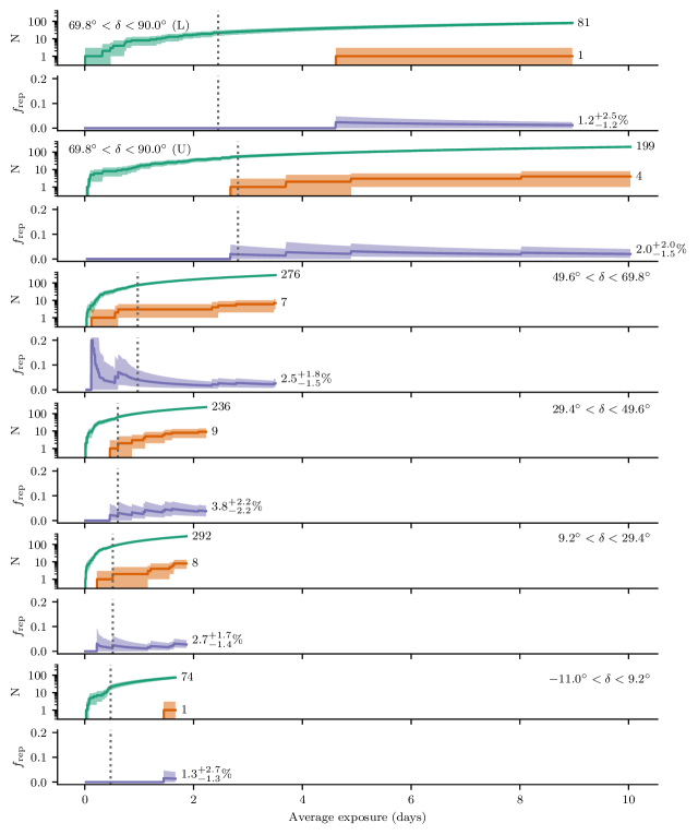
Figure 11: Fraction of repeating FRBs over all FRB sources, $f_{\mathrm{rep}}$, as a function of average total exposure in different declination bins (ranges are indicated in the top left or right corners, with U/L separating the “upper” and “lower” transit of the top bin, respectively) with approximately equal exposure and sensitivity within each bin. In each pair of panels the first shows the number of FRB (green) and repeater (orange) sources and the second value of $f_{\mathrm{rep}}$ (purple) with the values at 2021 May 1 written out (90% confidence). The FRB rate is extrapolated after the cutoff date (gray dotted line) for the first catalog. This figure includes only detections with S/N $>12$.

Shin et al. (2023) used a detailed population synthesis to infer a volumetric rate of of $7.3\times 10^{4}$ bursts Gpc^-3 year^-1 above a pivot energy of $10^{39}$ erg and below a scattering timescale of 10 ms at 600 MHz based on FRBs in CHIME/FRB’s first catalog. Based on the observed $f_{\mathrm{rep}}$ in CHIME/FRB, the rate of active repeating sources can only be a few percent of that rate. Without an analogous population synthesis accounting for the observed $f_{\mathrm{rep}}$, we cannot make any firm conclusions about the statistics of the population of repeating FRBs versus a putative distinct population of truly one-off events. It is also not possible to compare $f_{\mathrm{rep}}$ as measured for the CHIME/FRB survey with $f_{\mathrm{rep}}$ in other surveys because other repeating sources of FRBs were discovered in targeted follow-up observations rather than untargeted observations (Spitler et al., 2016; Kumar et al., 2019; Luo et al., 2020; Kumar et al., 2021; Niu et al., 2022).

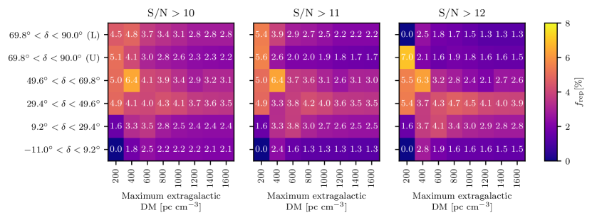
Figure 12: Evolution of $f_{\mathrm{rep}}$ (in %) in six declination bins as a function of maximum extragalactic DM (NE2001) for three different S/N thresholds. While there are hints of trends towards higher $f_{\mathrm{rep}}$ at lower maximum extragalactic DM and closer to zenith ($\delta=$49.6°), note that uncertainties are not shown here and that all values are consistent at the 90% confidence level.

4.6 Do All FRBs Repeat?

Even though multiple lines of evidence point to observed differences between the properties of repeater bursts and apparently one-off events, it is not yet possible to rule out that all FRBs repeat. Detailed population synthesis studies are necessary to properly interpret observations and rule out selection effects as the origins of the observed differences.

There is an observed dichotomy between the burst durations and bandwidths of repeater bursts and apparently one-off events (Pleunis et al., 2021b) that persists in this new sample (§3.3). To this, we add an observed difference in DM distributions (§3.3.2) but no detectable bimodality in repeat rates (§4.4). We find a significant correlation between burst width and repetition rate only if we include candidate repaters in the analysis, which might point to an evolution of burst properties with rate (§4.4). Only 2.6% of sources detected by CHIME/FRB has so far been seen to repeat.

Reconciling the dichotomy in burst morphology with one population of repeating FRBs with a continuum of repetition rates needs a correlation between repetition rate and burst duration (potentially observed; §4.4) and anti-correlation between repetition rate and bandwidth (not yet observed). This could either be achieved intrinsically through the emission mechanism or extrinsically through a propagation effect (e.g., tied to an evolutionary stage if active repeaters are young sources). Beaming geometry could provide a correlation between repetition and duration as wider opening angles could make bursts from sources both easier to detect and longer in duration (Connor et al., 2020). However, it is unclear how a wider opening angle could also lead to narrower emission bandwidths.

Studies of the host galaxies (Bhandari et al., 2022) and galaxy offsets (Mannings et al., 2021) of FRBs have not found clear differences between those of repeating sources and one-off events, except that the hosts of repeaters FRBs 20121102A and 20190520B are outliers in the currently known population.

An additional future probe of differences could be polarization properties, as more polarization properties of one-off events become available. On the other hand, there already exists an observed wide diversity in the polarization properties of the repeaters (e.g., Mckinven et al., 2022b).

Matching the observables to an astrophysical population of FRBs requires population synthesis. This has been used previously to constrain the repetition statistics and energy function of repeaters (Caleb et al., 2019; James et al., 2020a, b; Lu et al., 2020) and, for CHIME/FRB data, to interpret the scattering timescales of FRBs in the first catalog (Chawla et al., 2022). A publicly available general framework for population synthesis is provided by frbpoppy (Gardenier et al., 2021). Here, we outline some considerations for accurately modeling FRBs with CHIME/FRB observations for future population studies.

When modeling repeaters and one-off events as distinct populations, many new variables are introduced. Apart from separate volumetric rates, it needs to be carefully considered whether they share other population model parameters, such as those describing their energy function, evolution through cosmic time, and spectral properties. Shin et al. (2023) fit an energy function and volumetric rate to CHIME/FRB’s first catalog. As $\sim$90% of FRBs in the first catalog are one-off events, it is likely that those measurements could be used well to model one-off events. Those and other model fits are, however, sensitive to the inclusion of repeating sources for which only one event has been detected as apparent nonrepeaters. There is also the question of how to model the burst rates of repeaters, as varying levels of burst activity have been observed across the population of identified repeating FRBs, including highly clustered and rarely repeating sources (§4.4; see also, e.g., Oppermann et al., 2018; Good et al., 2023; Nimmo et al., 2023). Population synthesis will need to reproduce the observed distribution of repetition rates, while also reproducing the observed differences in other burst properties.

In addition to modeling the underlying intrinsic population, consideration also needs to be taken towards modeling the survey in which these bursts were detected and comparing the modeled population bursts with the observed data. For this, modeling selection effects is crucial. To accurately forward-model the CHIME/FRB survey, it is important to take into account its exposure and to use a beam model. The CHIME/FRB synthesized beams have chromatic sensitivities set by the primary beam response of the CHIME telescope and the beamforming algorithm, which can lead to, e.g., apparent, observed, bandwidths that are smaller than intrinsic bandwidths if bursts are detected away from the centers of beams (see, e.g., §2.1.3 and Fig. 2 in Pleunis et al., 2021b). The selection function of the CHIME/FRB detection pipeline has been characterized with injections and has been made publicly available (Merryfield et al., 2023). The strongest bias of the detection pipeline is against bursts with scattering timescales above 10 ms at 600 MHz (CHIME/FRB Collaboration et al., 2021).

5 Conclusions

We have presented 25 new repeating sources of FRBs, plus 14 additional candidate repeaters, from a complete search of the CHIME/FRB database from the start of operations on 2019 September 3 up to 2021 May 1. This brings the total number of repeating FRBs discovered by the CHIME/FRB project to 46, or counting the candidates, 60. This large bounty is a result of CHIME’s large field-of-view, high sensitivity, and daily surveying of a large area of sky. Additional repeater discoveries continue to be made by CHIME/FRB at a steady pace.

The DMs of the confirmed sources reported on in this paper fall in the range $\sim$200–1700 pc cm^-3. Combining these with the DMs of previously reported CHIME/FRB repeaters, we have now demonstrated that on average, the DMs of repeaters are lower than those of the apparently nonrepeating sources found by CHIME/FRB. This seems likely to be at least partly an observational bias, since, for reasonable luminosity functions, nearby repeaters will be found preferentially. However, it may also signal a distinct astrophysical origin for repeaters versus nonrepeating sources; detailed population synthesis studies that account for the many observational and instrumental biases will be required to disentangle such effects. The possibility of distinct physical origins is supported but unproven by statistically different dynamic spectra between the two groups – wider bursts and narrower spectra for repeaters – as previously shown (CHIME/FRB Collaboration et al., 2021; Pleunis et al., 2021b), a result which is strongly supported by our analysis of our now much larger sample.

Interestingly, we have detected no significant bimodality in the repeat rates of repeaters and apparent nonrepeaters, although the most active CHIME/FRB repeaters do have anomalously high rates compared to the bulk of the studied population. While we measure that $2.6_{-2.6}^{+2.9}$% of sources detected by CHIME/FRB repeat, the lack of bimodality in burst rates between the populations suggests that some fraction of our apparent nonrepeaters may yet repeat and that we cannot rule out all FRBs eventually repeating.

We encourage radio and multi-wavelength follow-up of the newly presented sources, and especially of our candidates. As for previously published repeaters, we update a webpage with new detections of these sources to communicate which sources are active while also continuing to provide the community with realtime events via VOEvents.

Appendix A Candidate repeating sources of fast radio bursts

Source properties of 14 candidate repeating source of FRBs are summarized in Table 3. The dynamic spectra of their bursts are shown in Figure 13. These candidates have lower significance, which by definition means the burst-to-burst DM and sky position differences are larger and the repetition rates are low. The DM differences are as large as $\sim$14 pc cm^-3 (candidate FRBs 20190107B and 20200320A) and variation of this magnitude has not yet been observed in repeating sources of FRBs before. Some of the bursts in this candidate sample show larger than average bandwidths for repeater bursts, which we caution to overinterpret (i.e., we do not downweight their likelihood as candidates for this reason and we do not claim a correlation between bandwidth and repetition rate using this candidate sample). Some candidate sources also show apparently different scattering timescales from burst to burst (candidate FRBs 20190328C, 20201105A, 20200828A, 20210203E and 20190127B) that we cannot at this time confirm are real. Scattering variations have been detected in FRB 20190520B (Ocker et al., 2023).

Table 3: Properties of 14 New Candidate Repeating Sources of FRBs, Ordered by Increasing $R_{\mathrm{cc}}$ (Our “Silver” Sample)

FRB Sourcea	$R_{\mathrm{cc}}$	$\alpha^{b}$	$\delta^{b}$	$l^{c}$	$b^{c}$	DMd	DM${}_{\rm NE2001}^{e}$	DM${}_{\rm YMW16}^{e}$	Nbursts	Exposuref	Completenessg	Burst rateh
		(J2000)	(J2000)	(deg)	(deg)	(pc cm-3)	(pc cm-3)	(pc cm-3)		(hr, upper / lower)	(Jy ms)	(hr-1)
20190303D	$0.62$	185.34(7)	70.69(2)	$126.5$	$46.2$	714.552(8)	37	29	2	$55\pm 44$ / $142\pm 3$	2.8 / 16.7	$(1.49_{-1.71}^{+3.42})\times 10^{-2}$
20181201D	$0.64$	267(1)	89.12(1)	$122.0$	$27.4$	443.849(2)	54	51	2	$3591\pm 288$ / $4359\pm 14$	2.7 / 4.2	$(2.24_{-1.85}^{+4.81})\times 10^{-4}$
20190328C	$0.71$	$75.65_{-0.37}^{+0.10}$	$82.11_{-0.19}^{+0.24}$	$130.6$	$23.3$	472.819(8)	64	67	2	$311\pm 161$ / $294\pm 161$	1.8 / 5.7	$(7.16_{-7.74}^{+27.10})\times 10^{-4}$
20191105Bi	$0.73$	84.11(6)	72.52(2)	$140.6$	$20.4$	311.226(2)	74	84	2	$163\pm 15$ / $161\pm 0$	3.1 / 51.1	$(5.9_{-4.9}^{+12.7})\times 10^{-3}$
20190107Bj	$0.78$	$49.31_{-0.11}^{+1.18}$	$83.40_{-0.72}^{+0.13}$	$127.1$	$21.8$	168.253(3)	68	73	2	$362\pm 189$ / $329\pm 196$	0.2 / 0.4	$(1.91_{-2.06}^{+7.20})\times 10^{-5}$
		$22.37_{-0.80}^{+0.27}$	$83.37_{-0.39}^{+0.08}$	$124.1$	$20.6$		72	81
20200320A	$0.92$	$42.45_{-0.04}^{+0.02}$	$15.84_{-0.06}^{+0.07}$	$160.2$	$-38.3$	593.524(2)	46	39	2	$59\pm 11$	$8.7$	$(3.91_{-3.78}^{+14.60})\times 10^{-2}$
20190210C	$1$	$313.90_{-0.26}^{+0.13}$	$89.19_{-0.47}^{+0.21}$	$122.2$	$26.7$	643.365(2)	54	51	2	$3354\pm 1180$ / $3086\pm 959$	1.7 / 2.6	$<$ 1.83$\times 10^{-4}$
20190812A	$1.4$	$268.05_{-0.11}^{+0.22}$	$50.71_{-0.02}^{+0.02}$	$78.1$	$29.8$	252.889(2)	48	41	2	$81\pm 26$	$0.9$	$(1.85_{-1.63}^{+4.01})\times 10^{-3}$
20200828A	$1.6$	$114.08_{-0.20}^{+0.44}$	$80.02_{-0.11}^{+0.09}$	$134.1$	$28.6$	555.41(2)	54	50	2	$241\pm 133$ / $223\pm 129$	0.4 / 1.6	$(1.89_{-1.88}^{+4.20})\times 10^{-4}$
20190905A	$2.2$	$73.27_{-0.03}^{+0.06}$	$88.24_{-0.06}^{+0.07}$	$124.6$	$26.2$	231.5577(7)	57	55	2	$5399\pm 980$ / $3928\pm 1313$	0.4 / 0.6	$(9.99_{-8.41}^{+21.50})\times 10^{-6}$
20190127B	$2.7$	$169.26_{-0.08}^{+0.06}$	$83.51_{-0.08}^{+0.08}$	$126.0$	$33.0$	678.350(3)	48	42	2	$345\pm 191$ / $358\pm 197$	0.1 / 0.3	(7${}_{-8}^{+27})\times 10^{-6}$
20210323C	$3$	$122.07_{-0.38}^{+0.11}$	$72.35_{-0.14}^{+0.39}$	$142.6$	$31.6$	288.6(3)	50	45	3	$135\pm 78$ / $108\pm 60$	3.6 / 31.8	$(1.37_{-1.27}^{+2.30})\times 10^{-2}$
20180909A	$3.9$	$120.04_{-0.17}^{+0.30}$	$57.00_{-0.07}^{+0.06}$	$160.6$	$31.7$	418.52(4)	52	49	2	$75\pm 45$	$0.1$	$(3.35_{-3.41}^{+7.48})\times 10^{-5}$
20200508H	$4$	$54.60_{-0.27}^{+0.49}$	$88.04_{-0.38}^{+0.32}$	$124.4$	$25.7$	479.430(6)	58	57	2	$1296\pm 537$ / $1395\pm 375$	0.8 / 1.1	$(1.04_{-0.96}^{+2.27})\times 10^{-4}$

^a Here we employ the TNS naming convention, see https://www.wis-tns.org/astronotes/astronote/2020-70.
^b Positions were determined from baseband data where available and from per-burst S/N data otherwise (see §3.1), uncertainties are at 90% confidence.
^c Galactic longitude and latitude for the best position.
^d Inverse-variance-weighted average DM, and the uncertainty in the calculation of that average. In cases where the DM was fixed in the fitburst fit, we set the DM uncertainty to 0.5 pc cm^-3 for the calculation of the average. For candidates with large DM variation from burst to burst, this average and its uncertainty may not necessarily be representative and we advise looking at the individual burst DMs using generous DM ranges when conducting follow-up searches of these candidates.
^e Maximum model prediction along this line-of-sight for the NE2001 (Cordes & Lazio, 2002) and YMW16 (Yao et al., 2017) Galactic electron density distribution models. Neither model accounts for DM contributions from the Galactic halo, which contributes no more than 111 pc cm^-3 (Cook et al., 2023).
^f For sources observed twice a day, the second entry corresponds to the less sensitive lower transit. The uncertainties in the total exposure for the upper and lower transits of each source are dominated by the corresponding source declination uncertainties since the widths of the synthesized beams vary significantly with declination.
^g Fluence completeness limits are given at the 90% confidence level. For sources observed twice a day, the second entry corresponds to the less sensitive lower transit.
^h Adjusted to a 5 Jy ms fluence threshold, assuming a $-1.5$ power-law energy index.
ⁱ The best-known sky position of this source falls in between the FWHMs at 600 MHz of the synthesized beams. We report the exposure at the beam centre of the nearest beam and have scaled the fluence completeness threshold accordingly.
^j Two equally likely “islands” in the localization 90% confidence region.

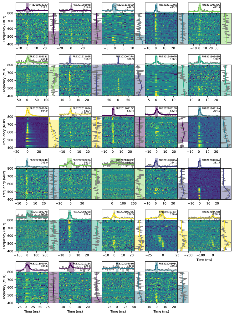
Figure 13: Same as Figure 5, but for candidate repeating sources of FRBs (i.e., “silver” sample).

Appendix B Burst Rates for Previously Published Repeaters

Table 4: Updated Burst Rates for Previously Published Repeaters

FRB Source	Reference	Burst Ratea
		(hr-1)
20180814A	CHIME/FRB Collaboration et al. (2019a)	$(6.57_{-4.47}^{+5.09})\times 10^{-1}$
20180916B	CHIME/FRB Collaboration et al. (2019b)	$(4.48_{-0.86}^{+1.00})\times 10^{-1}$
20181030A	CHIME/FRB Collaboration et al. (2019b)	$(1.48_{-1.32}^{+2.47})\times 10^{-3}$
20181128A	CHIME/FRB Collaboration et al. (2019b)	$(4.08_{-2.70}^{+4.63})\times 10^{-2}$
20181119A	CHIME/FRB Collaboration et al. (2019b)	$(6.77_{-4.16}^{+5.95})\times 10^{-2}$
20190116A	CHIME/FRB Collaboration et al. (2019b)	$(3.18_{-2.62}^{+6.83})\times 10^{-2}$
20181017A	CHIME/FRB Collaboration et al. (2019b)	$(1.05_{-1.16}^{+3.97})\times 10^{-2}$
20190209A	CHIME/FRB Collaboration et al. (2019b)	$(6.95_{-6.96}^{+15.50})\times 10^{-3}$
20190222A	CHIME/FRB Collaboration et al. (2019b)	$(1.44_{-1.19}^{+3.09})\times 10^{-2}$
20190208A	Fonseca et al. (2020)	$(4.34_{-2.30}^{+3.81})\times 10^{-2}$
20190604A	Fonseca et al. (2020)	$(7.96_{-6.55}^{+17.10})\times 10^{-3}$
20190212A	Fonseca et al. (2020)	$(3.36_{-2.65}^{+4.08})\times 10^{-2}$
20180908B	Fonseca et al. (2020)	$(4.11_{-0.30}^{+6.52})\times 10^{-2}$
20190117A	Fonseca et al. (2020)	$(2.15_{-1.21}^{+2.09})\times 10^{-1}$
20190303A	Fonseca et al. (2020)	$(1.46_{-0.49}^{+0.64})\times 10^{-1}$
20190417A	Fonseca et al. (2020)	$(9.05_{-3.71}^{+5.35})\times 10^{-2}$
20190213A	Fonseca et al. (2020)	$(3.84_{-3.88}^{+8.56})\times 10^{-2}$
20190907A	Fonseca et al. (2020)	$(2.98_{-1.73}^{+2.93})\times 10^{-2}$
20200120E	Bhardwaj et al. (2021a)	–
20201124A	Lanman et al. (2022)	3.28${}_{-1.06}^{+1.41}$
20171019A	Kumar et al. (2019)	–

^a Adjusted to a 5 Jy ms fluence threshold, assuming a $-1.5$ power-law energy index. No rate measurements are reported for FRBs 20200120E and 20171019A as the sensitivity of the CHIME/FRB system to their source locations has not been measured (§4.4).

Appendix C Description of Fields in Catalog

In Table LABEL:ta:catalog_descriptions, we provide descriptions for each field present in our repeater catalog.

Table 5: Repeater Catalog Field Descriptions

Column Number	Unit	Column Name	Description
0	…	tns_name	TNS name
1	…	previous_name	Previous name (if applicable)
2	…	repeater_name	Associated repeater name
3	degrees	ra_1	Right ascension (J2000; first likelihood contour; see §3.1)
4	degrees	ra_1_err_low	Right ascension lower error (see §3.1; first likelihood contour)
5	degrees	ra_1_err_up	Right ascension upper error (see §3.1; first likelihood contour)
6	degrees	ra_2	Right ascension (J2000; second likelihood contour; see §3.1)
7	degrees	ra_2_err_low	Right ascension lower error (see §3.1; second likelihood contour)
8	degrees	ra_2_err_up	Right ascension upper error (see §3.1; second likelihood contour)
9	…	ra_notes	Notes on right ascension
10	degrees	dec_1	Declination (J2000; first likelihood contour; see §3.1)
11	degrees	dec_1_err_low	Declination lower error (see §3.1; first likelihood contour)
12	degrees	dec_1_err_up	Declination upper error (see §3.1; first likelihood contour)
13	degrees	dec_2	Declination (J2000; second likelihood contour; see §3.1)
14	degrees	dec_2_err_low	Declination lower error (see §3.1; second likelihood contour)
15	degrees	dec_2_err_up	Declination upper error (see §3.1; second likelihood contour)
16	…	dec_notes	Notes on declination
17	degrees	gl	Galactic longitude
18	degrees	gb	Galactic latitude
19	hour	exp_up	Exposure for upper transit of the source
20	hour	exp_up_err	Exposure error for upper transit of the source
21	…	exp_up_notes	Notes on exposure for upper transit of the source
22	hour	exp_low	Exposure for lower transit of the source
23	hour	exp_low_err	Exposure error for lower transit of the source
24	…	exp_low_notes	Notes on exposure for lower transit of the source
25	…	bonsai_snr	Detection S/N
26	pc cm-3	bonsai_dm	Detection DM
27	Jy ms	low_ft_90	Lower limit fluence threshold (90$\%$ confidence)
28	Jy ms	up_ft_90	Upper limit fluence threshold (90$\%$ confidence)
29	Jy ms	low_ft_95	Lower limit fluence threshold (95$\%$ confidence)
30	Jy ms	up_ft_95	Upper limit fluence threshold (95$\%$ confidence)
31	…	snr_fitb	S/N determined using the fitting algorithm fitburst
32	pc cm-3	dm_fitb	DM determined using the fitting algorithm fitbursta
33	pc cm-3	dm_fitb_err	DM error determined using the fitting algorithm fitbursta
34	pc cm-3	dm_exc_1_ne2001	DM excess between DM determined by fitburst and NE2001 assuming the first likelihood sky position of the source
35	pc cm-3	dm_exc_2_ne2001	DM excess between DM determined by fitburst and NE2001 assuming the second likelihood sky position of the source
36	pc cm-3	dm_exc_1_ymw16	DM excess between DM determined by fitburst and YMW16 assuming the first likelihood sky position of the source
37	pc cm-3	dm_exc_2_ymw16	DM excess between DM determined by fitburst and YMW16 assuming the second likelihood sky position of the source
38	s	bc_width	Boxcar width of the pulse (including all sub-bursts)
39	s	scat_time	Scattering time at 600 MHza
40	s	scat_time_err	Scattering time errora
41	Jy	flux	Peak flux of the band-average profile (lower limit)
42	Jy	flux_err	Flux error
43	…	flux_notes	Notes on the burst flux
44	Jy ms	fluence	Fluence (lower limit)
45	Jy ms	fluence_err	Fluence error
46	…	fluence_notes	Notes on the burst fluence
47	…	sub_num	Sub-burst number (if applicable). If the FRB has only one burst, then the sub-burst number is 0. Sub-bursts listed in chronological order.
48	MJD	mjd_400	Time of arrival with reference to 400.1953125 MHz for the specific sub-burst.
49	MJD	mjd_400_err	Time of arrival error with reference to 400.1953125 MHz for the specific sub-burst.
50	MJD	mjd_inf	Time of arrival with reference to infinite frequency for the specific sub-burst.
51	MJD	mjd_inf_err	Time of arrival error with reference to infinite frequency for the specific sub-burst.
52	s	width_fitb	Width of sub-burst using fitburst
53	s	width_fitb_err	Width error of sub-burst using fitburst
54	…	sp_idx	Spectral index for the sub-burst
55	…	sp_idx_err	Spectral index error for the sub-burst
56	…	sp_run	Spectral running for the sub-burst
57	…	sp_run_err	Spectral running error for the sub-burst
58	MHz	high_freq	Highest frequency band of detection for the sub-burst at FWTM
59	MHz	low_freq	Lowest frequency band of detection for the sub-burst at FWTM
60	MHz	peak_freq	Peak frequency of detection for the sub-burst
61	…	chi_sq	Chi-squared from fitburst
62	…	dof	Number of degrees of freedom in fitburst
63	…	flag_frac	Fraction of spectral channels flagged in fitburst
64	…	r_cc	Contamination rate (see Section 2.2.2).

Appendix D Additional Figures

References

- Aggarwal (2021) Aggarwal, K. 2021, ApJ, 920, L18
- Ai et al. (2021) Ai, S., Gao, H., & Zhang, B. 2021, ApJ, 906, L5
- Anna-Thomas et al. (2022) Anna-Thomas, R., Connor, L., Burke-Spolaor, S., et al. 2022, arXiv e-prints, arXiv:2202.11112
- Astropy Collaboration et al. (2013) Astropy Collaboration, Robitaille, T. P., Tollerud, E. J., et al. 2013, A&A, 558, A33
- Astropy Collaboration et al. (2018) Astropy Collaboration, Price-Whelan, A. M., Sipőcz, B. M., et al. 2018, AJ, 156, 123
- Astropy Collaboration et al. (2022) Astropy Collaboration, Price-Whelan, A. M., Lim, P. L., et al. 2022, ApJ, 935, 167
- Bandura et al. (2014) Bandura, K., Addison, G. E., Amiri, M., et al. 2014, in Society of Photo-Optical Instrumentation Engineers (SPIE) Conference Series, Vol. 9145, Ground-based and Airborne Telescopes V
- Behnel et al. (2011) Behnel, S., Bradshaw, R., Citro, C., et al. 2011, Computing in Science & Engineering, 13, 31
- Bethapudi et al. (2022) Bethapudi, S., Spitler, L. G., Main, R. A., Li, D. Z., & Wharton, R. S. 2022, arXiv e-prints, arXiv:2207.13669
- Bhandari et al. (2022) Bhandari, S., Heintz, K. E., Aggarwal, K., et al. 2022, AJ, 163, 69
- Bhardwaj et al. (2021a) Bhardwaj, M., Gaensler, B. M., Kaspi, V. M., et al. 2021a, ApJ, 910, L18
- Bhardwaj et al. (2021b) Bhardwaj, M., Kirichenko, A. Y., Michilli, D., et al. 2021b, ApJ, 919, L24
- Bochenek et al. (2020) Bochenek, C. D., Ravi, V., Belov, K. V., et al. 2020, Nature, 587, 59
- Caleb et al. (2019) Caleb, M., Stappers, B. W., Rajwade, K., & Flynn, C. 2019, MNRAS, 484, 5500
- Caleb et al. (2020) Caleb, M., Stappers, B. W., Abbott, T. D., et al. 2020, MNRAS, 496, 4565
- Cassanelli et al. (2022) Cassanelli, T., Leung, C., Rahman, M., et al. 2022, AJ, 163, 65
- Chawla et al. (2020) Chawla, P., Andersen, B. C., Bhardwaj, M., et al. 2020, ApJ, 896, L41
- Chawla et al. (2022) Chawla, P., Kaspi, V. M., Ransom, S. M., et al. 2022, ApJ, 927, 35
- CHIME Collaboration et al. (2022) CHIME Collaboration, Amiri, M., Bandura, K., et al. 2022, ApJS, 261, 29
- CHIME/FRB Collaboration et al. (2018) CHIME/FRB Collaboration, Amiri, M., Bandura, K., et al. 2018, ApJ, 863, 48
- CHIME/FRB Collaboration et al. (2019a) —. 2019a, Nature, 566, 235
- CHIME/FRB Collaboration et al. (2019b) CHIME/FRB Collaboration, Andersen, B. C., Bandura, K., et al. 2019b, ApJ, 885, L24
- CHIME/FRB Collaboration et al. (2020a) CHIME/FRB Collaboration, Andersen, B. C., Bandura, K. M., et al. 2020a, Nature, 587, 54
- CHIME/FRB Collaboration et al. (2020b) CHIME/FRB Collaboration, Amiri, M., Andersen, B. C., et al. 2020b, Nature, 582, 351
- CHIME/FRB Collaboration et al. (2021) —. 2021, ApJS, 257, 59
- CHIME/Pulsar Collaboration et al. (2021) CHIME/Pulsar Collaboration, Amiri, M., Bandura, K. M., et al. 2021, ApJS, 255, 5
- Connor (2019) Connor, L. 2019, MNRAS, 487, 5753
- Connor et al. (2020) Connor, L., Miller, M. C., & Gardenier, D. W. 2020, MNRAS, 497, 3076
- Connor & Petroff (2018) Connor, L., & Petroff, E. 2018, ApJ, 861, L1
- Cook et al. (2023) Cook, A. M., Bhardwaj, M., Gaensler, B. M., et al. 2023, arXiv e-prints, arXiv:2301.03502
- Cordes & Chatterjee (2019) Cordes, J. M., & Chatterjee, S. 2019, ARA&A, 57, 417
- Cordes & Lazio (2002) Cordes, J. M., & Lazio, T. J. W. 2002, arXiv preprint astro-ph/0207156
- Cruces et al. (2021) Cruces, M., Spitler, L. G., Scholz, P., et al. 2021, MNRAS, 500, 448
- Desvignes et al. (2018) Desvignes, G., Eatough, R. P., Pen, U. L., et al. 2018, ApJ, 852, L12
- Dong et al. (2022) Dong, F. A., Crowter, K., Meyers, B. W., et al. 2022, arXiv e-prints, arXiv:2210.09172
- Ester et al. (1996) Ester, M., Kriegel, H.-P., Sander, J., & Xu, X. 1996, in Proceedings of the Second International Conference on Knowledge Discovery and Data Mining, KDD’96 (AAAI Press), 226–231
- Feng et al. (2022) Feng, Y., Li, D., Yang, Y.-P., et al. 2022, Science, 375, 1266
- Fonseca et al. (2020) Fonseca, E., Andersen, B. C., Bhardwaj, M., et al. 2020, ApJ, 891, L6
- Gajjar et al. (2018) Gajjar, V., Siemion, A. P. V., Price, D. C., et al. 2018, ApJ, 863, 2
- Gardenier et al. (2021) Gardenier, D. W., Connor, L., van Leeuwen, J., Oostrum, L. C., & Petroff, E. 2021, A&A, 647, A30
- Goeman & Solari (2014) Goeman, J. J., & Solari, A. 2014, Statistics in Medicine, 33, 1946. https://onlinelibrary.wiley.com/doi/abs/10.1002/sim.6082
- Good et al. (2023) Good, D. C., Chawla, P., Fonseca, E., et al. 2023, ApJ, 944, 70
- Górski et al. (2005) Górski, K. M., Hivon, E., Banday, A. J., et al. 2005, ApJ, 622, 759
- Hardy et al. (2017) Hardy, L. K., Dhillon, V. S., Spitler, L. G., et al. 2017, MNRAS, 472, 2800
- Harrington & Fleming (1982) Harrington, D. P., & Fleming, T. R. 1982, Biometrika, 69, 553. https://doi.org/10.1093/biomet/69.3.553
- Harris et al. (2020) Harris, C. R., Millman, K. J., van der Walt, S. J., et al. 2020, Nature, 585, 357. https://doi.org/10.1038/s41586-020-2649-2
- Helsel (2005) Helsel, D. R. 2005, Nondetects and data analysis. Statistics for censored environmental data. (Wiley-Interscience)
- Hessels et al. (2019) Hessels, J. W. T., Spitler, L. G., Seymour, A. D., et al. 2019, ApJ, 876, L23
- Hilmarsson et al. (2021) Hilmarsson, G. H., Michilli, D., Spitler, L. G., et al. 2021, ApJ, 908, L10
- Hunter (2007) Hunter, J. D. 2007, Computing in Science & Engineering, 9, 90
- James et al. (2020a) James, C. W., Osłowski, S., Flynn, C., et al. 2020a, ApJ, 895, L22
- James et al. (2020b) —. 2020b, MNRAS, 495, 2416
- Josephy et al. (2019) Josephy, A., Chawla, P., Fonseca, E., et al. 2019, ApJ, 882, L18
- Josephy et al. (2021) Josephy, A., Chawla, P., Curtin, A. P., et al. 2021, ApJ, 923, 2
- Kirsten et al. (2022) Kirsten, F., Marcote, B., Nimmo, K., et al. 2022, Nature, 602, 585
- Kumar et al. (2022) Kumar, P., Shannon, R. M., Lower, M. E., Deller, A. T., & Prochaska, J. X. 2022, arXiv e-prints, arXiv:2204.10816
- Kumar et al. (2019) Kumar, P., Shannon, R. M., Osłowski, S., et al. 2019, ApJ, 887, L30
- Kumar et al. (2021) Kumar, P., Shannon, R. M., Flynn, C., et al. 2021, MNRAS, 500, 2525
- Lanman et al. (2022) Lanman, A. E., Andersen, B. C., Chawla, P., et al. 2022, ApJ, 927, 59
- Law et al. (2022) Law, C. J., Connor, L., & Aggarwal, K. 2022, ApJ, 927, 55
- Law et al. (2017) Law, C. J., Abruzzo, M. W., Bassa, C. G., et al. 2017, ApJ, 850, 76
- Leung et al. (2021) Leung, C., Mena-Parra, J., Masui, K., et al. 2021, AJ, 161, 81
- Li et al. (2021) Li, D., Wang, P., Zhu, W. W., et al. 2021, Nature, 598, 267
- Lopaka (2020) Lopaka, L. 2020, NADA: Nondetects and Data Analysis for Environmental Data, r package version 1.6-1.1. https://CRAN.R-project.org/package=NADA
- Lu et al. (2020) Lu, W., Piro, A. L., & Waxman, E. 2020, MNRAS, 498, 1973
- Luo et al. (2020) Luo, R., Wang, B. J., Men, Y. P., et al. 2020, Nature, 586, 693
- Mannings et al. (2021) Mannings, A. G., Fong, W.-f., Simha, S., et al. 2021, ApJ, 917, 75
- Marcote et al. (2020) Marcote, B., Nimmo, K., Hessels, J. W. T., et al. 2020, Nature, 577, 190
- Masui (2017) Masui, K. 2017, Bitshuffle: Filter for improving compression of typed binary data, Astrophysics Source Code Library, record ascl:1712.004, , , ascl:1712.004
- McKinney (2010) McKinney, W. 2010, in Proceedings of the 9th Python in Science Conference, ed. Stéfan van der Walt & Jarrod Millman, 56–61
- Mckinven & CHIME/FRB Collaboration (2022) Mckinven, R., & CHIME/FRB Collaboration. 2022, The Astronomer’s Telegram, 15679, 1
- Mckinven et al. (2021) Mckinven, R., Michilli, D., Masui, K., et al. 2021, ApJ, 920, 138
- Mckinven et al. (2022a) Mckinven, R., Gaensler, B. M., Michilli, D., et al. 2022a, arXiv e-prints, arXiv:2205.09221
- Mckinven et al. (2022b) —. 2022b, ApJ
- Merryfield et al. (2023) Merryfield, M., Tendulkar, S. P., Shin, K., et al. 2023, AJ, 165, 152
- Michilli et al. (2018) Michilli, D., Seymour, A., Hessels, J. W. T., et al. 2018, Nature, 533, 132
- Michilli et al. (2021) Michilli, D., Masui, K. W., Mckinven, R., et al. 2021, ApJ, 910, 147
- Niino et al. (2022) Niino, Y., Doi, M., Sako, S., et al. 2022, ApJ, 931, 109
- Nimmo et al. (2021) Nimmo, K., Hessels, J. W. T., Keimpema, A., et al. 2021, Nature Astronomy, 5, 594
- Nimmo et al. (2022) Nimmo, K., Hessels, J. W. T., Kirsten, F., et al. 2022, Nature Astronomy, 6, 393
- Nimmo et al. (2023) Nimmo, K., Hessels, J. W. T., Snelders, M. P., et al. 2023, MNRAS, 520, 2281
- Niu et al. (2022) Niu, C. H., Aggarwal, K., Li, D., et al. 2022, Nature, 606, 873
- Ocker et al. (2023) Ocker, S. K., Cordes, J. M., Chatterjee, S., et al. 2023, MNRAS, 519, 821
- Oppermann et al. (2018) Oppermann, N., Yu, H.-R., & Pen, U.-L. 2018, MNRAS, 475, 5109
- Pastor-Marazuela et al. (2021) Pastor-Marazuela, I., Connor, L., van Leeuwen, J., et al. 2021, Nature, 596, 505
- Patel & CHIME/FRB Collaboration (2019) Patel, C., & CHIME/FRB Collaboration. 2019, The Astronomer’s Telegram, 13013, 1
- Petroff et al. (2019) Petroff, E., Hessels, J. W. T., & Lorimer, D. R. 2019, A&A Rev., 27, 4
- Pleunis (2021) Pleunis, Z. 2021, PhD thesis, McGill University
- Pleunis et al. (2021a) Pleunis, Z., Michilli, D., Bassa, C. G., et al. 2021a, ApJ, 911, L3
- Pleunis et al. (2021b) Pleunis, Z., Good, D. C., Kaspi, V. M., et al. 2021b, ApJ, 923, 1
- R Core Team (2020) R Core Team. 2020, R: A Language and Environment for Statistical Computing, R Foundation for Statistical Computing, Vienna, Austria. https://www.R-project.org/
- Rafiei-Ravandi & Smith (2022) Rafiei-Ravandi, M., & Smith, K. M. 2022, arXiv e-prints, arXiv:2206.07292
- Rajwade et al. (2020) Rajwade, K. M., Mickaliger, M. B., Stappers, B. W., et al. 2020, MNRAS, 495, 3551
- Scholz et al. (2020) Scholz, P., Cook, A., Cruces, M., et al. 2020, ApJ, 901, 165
- Shin et al. (2023) Shin, K., Masui, K. W., Bhardwaj, M., et al. 2023, ApJ, 944, 105
- Spitler et al. (2016) Spitler, L. G., Scholz, P., Hessels, J. W. T., et al. 2016, Nature, 531, 202
- Tavani et al. (2020) Tavani, M., Verrecchia, F., Casentini, C., et al. 2020, ApJ, 893, L42
- Tendulkar et al. (2017) Tendulkar, S. P., Bassa, C. G., Cordes, J. M., et al. 2017, ApJ, 834, L7
- The HDF Group (1997–2023) The HDF Group. 1997–2023, Hierarchical Data Format, version 5, , , https://www.hdfgroup.org/HDF5/
- The pandas development team (2020) The pandas development team. 2020, pandas-dev/pandas: Pandas 1.1.5, vv1.1.5, Zenodo, doi:10.5281/zenodo.4309786. https://doi.org/10.5281/zenodo.4309786
- Virtanen et al. (2020) Virtanen, P., Gommers, R., Oliphant, T. E., et al. 2020, Nature Methods, 17, 261
- Xu et al. (2022) Xu, H., Niu, J. R., Chen, P., et al. 2022, Nature, 609, 685
- Yao et al. (2017) Yao, J. M., Manchester, R. N., & Wang, N. 2017, ApJ, 835, 29
- Zonca et al. (2019) Zonca, A., Singer, L., Lenz, D., et al. 2019, Journal of Open Source Software, 4, 1298. https://doi.org/10.21105/joss.01298