Drawing Diestel-Leader graphs in 3D

Abstract

In this short note we give some code to represent Diestel-Leader graphs in 3D. The code is written in TikZ.

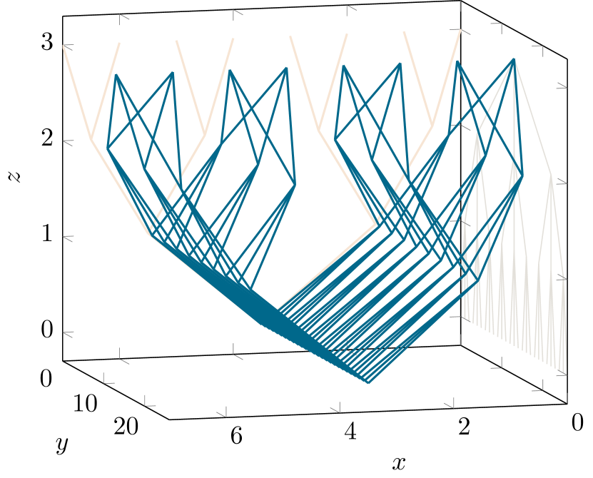
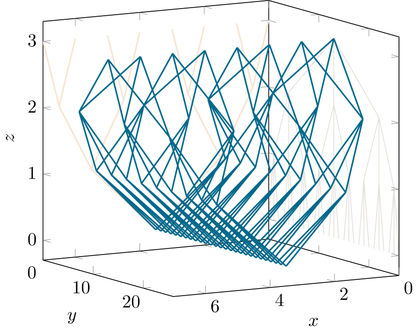
Figure 1: Two views of the Diestel-Leader graph $DL(3,2)$

The history of Diestel-Leader graphs takes its root in the following question asked by Woess [Woe91]: is every connected locally finite vertex-transitive graph quasi-isometric to some Cayley graph? In the hope of answering no to this question, Diestel and Leader [DL01] defined what we now call Diestel-Leader graphs. However it was only later, in the famous papers of Eskin, Fisher an Whyte [EFW07, EFW12] that it was showed that some of the aforementioned graphs are not quasi-isometric to any Cayley graph.

In this note we give a code to draw these graphs in 3D, using TikZ. Readers only interested by producing an illustration of some $DL(p,q)$ can jump to the last pages of this article (or the end of the .tex file) and copy-paste the code given in 2.2, write the wanted values of $p$ and $q$ (line 29) and then compile. Readers wishing to change the code can rely on the description made in Section 2.1. We start this note with a short reminder of the definition of Diestel-Leader graphs.

1 Diestel-Leader graphs

We recall here the definition of Diestel-Leader graphs. We refer to [Woe91, Section 2] for more details.

1.1 Tree and horocycles

Let $q\geq 2$ and denote by $\mathbf{T}=T_{q}$ the homogenous tree of degree $q+1$. Denote by $d$ the usual graph distance on $\mathbf{T}$ fixing to $1$ the length of an edge.

A geodesic ray is an infinite sequence $(v_{n})_{n\in\mathbb{N}}$ of vertices of $\mathbf{T}$ such that $d(v_{i},v_{j})=|i-j|$, for all $i,j\in\mathbb{N}$. We say that two rays are equivalent if ther symmetric difference is finite. We call end of $T_{q}$ an equivalence class of rays in $\mathbf{T}$ and denote by $\partial\mathbf{T}$ the space of ends of $\mathbf{T}$.

Let $\hat{\mathbf{T}}:=\partial\mathbf{T}\cup\mathbf{T}$. For any elements $x,y\in\hat{\mathbf{T}}$ there is a unique geodesic in $\hat{T}$, denoted by $\overline{xy}$, that connects $x$ and $y$.

Now fix an end $w\in\partial\mathbf{T}$, the confluent of two elements $x,y\in\hat{\mathbf{T}}\backslash{w}$ with respect to $w$, denoted by $x\curlywedge y$, is defined as the element $c=x\curlywedge y$ such that $\overline{xw}\cap\overline{yw}=\overline{cw}$, that is to say: the confluent is the point where the two geodesics $\overline{xw}$ and $\overline{yw}$ towards $w$ meet (see Figure 2).

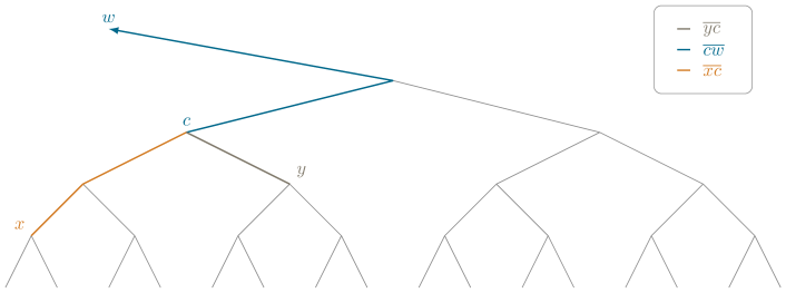
Figure 2: Example of the confluent of two points in $T_{2}$

Now, fix a root vertex $o\in\mathbf{T}$. We define below a Busemann function, which will allow us to endow our tree with some height notion.

Definition 1.1.

Let $w\in\partial T_{q}$. The Busemann function with respect to $w$ is the map $\mathfrak{h}:\mathbf{T}\rightarrow\mathbb{Z}$ defined by

$$\mathfrak{h}(x)=d(x,x\curlywedge o)-d(o,x\curlywedge o).$$

Example 1.2.

Let’s turn back to Figure 2 and let $o=y$ be the root. Then for $x$ represented in the figure, we have $x\curlywedge o=c$ and thus $d(x,x\curlywedge o)=2$ and $d(o,x\curlywedge o)=1$. Therefore $\mathfrak{h}(x)=1$.

Definition 1.3.

Let $w\in\partial T_{q}$ and $k\in\mathbb{N}$. The horocycle with respect to $w$, denoted by $H_{k}$, is the set $H_{k}=\left\{x\in\mathbf{T}:\mathfrak{h}(x)=k\right\}$.

We refer to Figure 3 for an illustration. Note that every horocycle in $\hat{T}$ is infinite. Every vertex $x$ in a horocycle $H_{k}$ has exactly one neighbour $x^{-}$ (called the predecessor) in $H_{k-1}$ and exactly $q$ neighbours (called successors) in $H_{k+1}$ (see Figure 3 for an illustration).

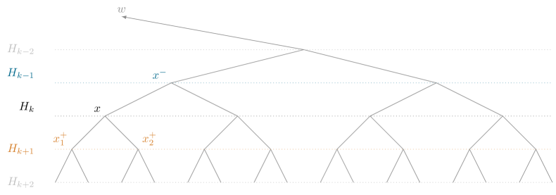
Figure 3: Horocycles, predecessor, successors

1.2 Diestel-Leader graphs

Now fix $p,q\geq 2$ and consider $T_{p}$ and $T_{q}$ with respective roots $o_{p}$ and $o_{q}$, and respective reference ends $w_{p}$ and $w_{q}$.

Definition 1.4.

The Diestel-Leader graph $DL(p,q)$ is the graph whith set of vertices

$$V\left(DL(p,q)\right)=\big{\{}(x,y)\in T_{p}\times T_{q}:\mathfrak{h}(x)=-\mathfrak{h}(y)\big{\}}.$$

and where there is an edge between two elements $(x_{1},y_{1})$ and $(x_{2},y_{2})$, if and only if $(x_{1},x_{2})$ is an edge in $T_{p}$ and $(y_{1},y_{2})$ is an edge in $T_{q}$.

If there is an edge between two vertices $(x_{1},y_{1})$ and $(x_{2},y_{2})$ in $DL(p,q)$, then remark that either

• $x_{2}$ is one of the $p$ childs of $x_{1}$ in $\mathbf{T}_{p}$ and in this case $y_{2}$ is the only predecessor of $y_{1}$ in $\mathbf{T}_{q}$, namely $y_{2}=y^{-}_{1}$ (see Figure 4(a));

• or $x_{2}=x^{-}_{1}$ is the unique predecessor of $x_{1}$ in $\mathbf{T}_{p}$ and in this case $y_{2}$ is one of the $q$ childs of $y_{1}$ in $\mathbf{T}_{q}$ (see Figure 4(b)).

We represent these two cases in Figure 4. The edge is drawn in blue, the $p$-regular tree in orange and the $q$-regular tree in brown. In light blue is represented the Diestel-Leader graph, we refer to Figure 5 for a drawing of $DL(p,q)$ itself. Note that in Figure 5, the corresponding $T_{p}$ and $T_{q}$ are drawn on the planes $x=0$ and $y=0$ respectively.

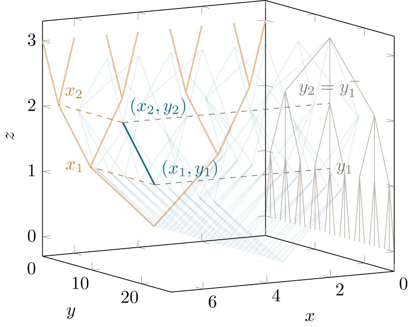
(a) When $x_{2}$ is a child of $x_{1}$ and $y_{2}=y^{-}_{1}$

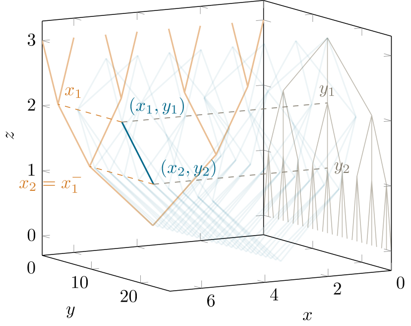
(b) When $y_{2}$ is a child of $y_{1}$ and $x_{2}=x^{-}_{1}$

Figure 4: Drawing an edge in $DL(p,q)$: two cases

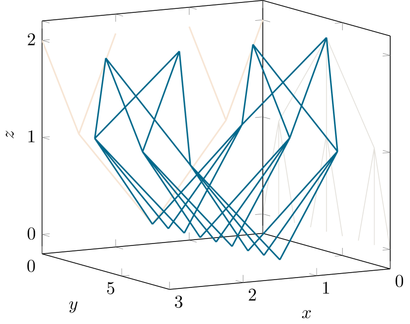
(a) $DL(3,2)$

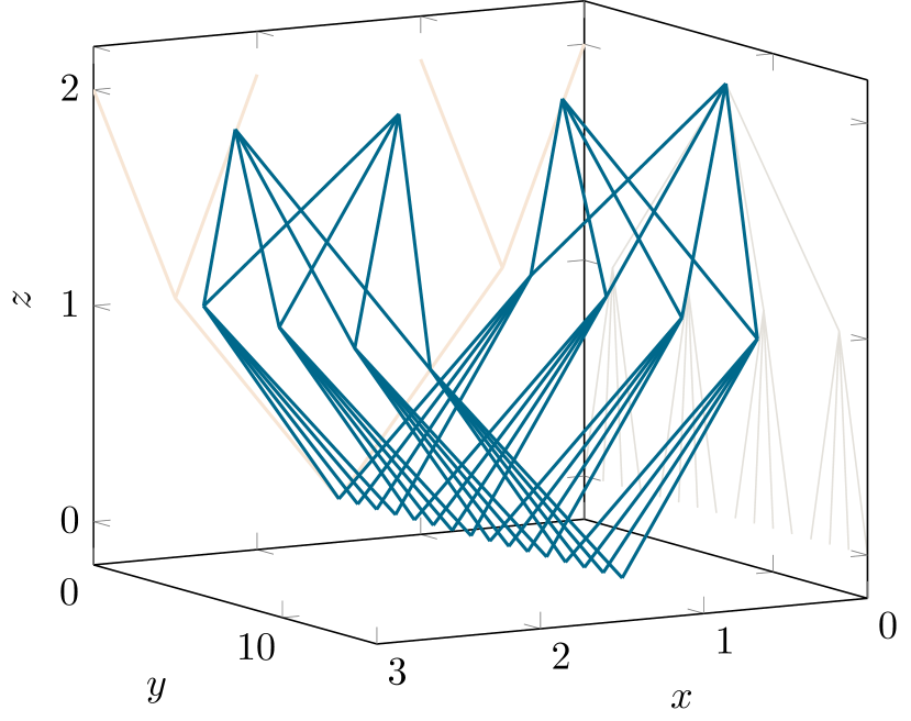
(b) $DL(4,2)$

Figure 5: Two different Diestel-Leader graphs, represented at the same scale

Remark 1.5.

When $p=q$ the graph $DL(p,q)$ is a Cayley graph of the Lamplighter group $\mathbb{Z}/p\mathbb{Z}\wr\mathbb{Z}$.

2 The code

The complete code is given in 2.2, and written in TikZ. We start by some comments on how the coordinates were computed and how the loops work.

2.1 Comments on the code

Variables

The main variables are \p, \q} (line 29) and \mintinlinelatex (line 35). The first two variables correspond to the number of childs in the first and the second tree respectively, that is to say the $p$ and $q$ in $DL(p,q)$. Finally, the height of the graph is parametrized by

\layers}:
there are \mintinline

latex$+1$ different heights of vertices appearing on the graph. With the values given in the example in 2.2, we produce the left image in Figure 1. Finally changing the values in view=16510 (line $17$) will change the point of view (see for example Figure 1). For more details on how to parametrize the view, see the pgfplots manual [Feu21, Section 4.11.1, page 311].

Structure of the code

The code is composed of one main loop cut in two parts: the first one that draws the tree on the plane $y=0$, and the second one that draws simultaneously the tree located on the plane $x=0$ and the Diestel-Leader graph. In this description “height” will stand for the $z$-coordinates in the picture.

Lines 58 to 72

We start by drawing the regular tree of degree $p$ represented on the plane $y=0$, in orange in the pictures. This tree grows from the bottom to the top. At height $h$ there are $p^{{\color[rgb]{0.4,0.6448,0.727}h}}$ vertices to draw and the space between two consecutive nodes at this height is ${\color[rgb]{0.5,0.5,0.5}\mathrm{pspace}}=p^{\text{layers-{\color[rgb]{0.4,0.6448,0.727}h}}}$ (in particular at the top, when ${\color[rgb]{0.4,0.6448,0.727}h}=layers$, the space between two nodes is equal to $1$). Moreover the first horizontal node at height ${\color[rgb]{0.4,0.6448,0.727}h}$ has for horizontal coordinates the middle of $[0,p^{\mathrm{layers}-{\color[rgb]{0.4,0.6448,0.727}h}}-1]$ that is to say

$$p^{\mathrm{layers}-{\color[rgb]{0.4,0.6448,0.727}h}}/2-0.5={\color[rgb]{0.5,0.5,0.5}\mathrm{pspace}}/2-0.5,$$

and therefore, if ${\color[rgb]{0.4,0.6448,0.727}h}\neq layers$, the first of its child (at height ${\color[rgb]{0,.408,.545}n}={\color[rgb]{0.4,0.6448,0.727}h}+1$) has coordinates the middle of $[0,p^{\mathrm{layers}-{\color[rgb]{0,.408,.545}n}}-1]$, namely $p^{\mathrm{layers}-{\color[rgb]{0.4,0.6448,0.727}h}}/(2p)-0.5={\color[rgb]{0.5,0.5,0.5}\mathrm{pspace}}/(2p)-0.5$.

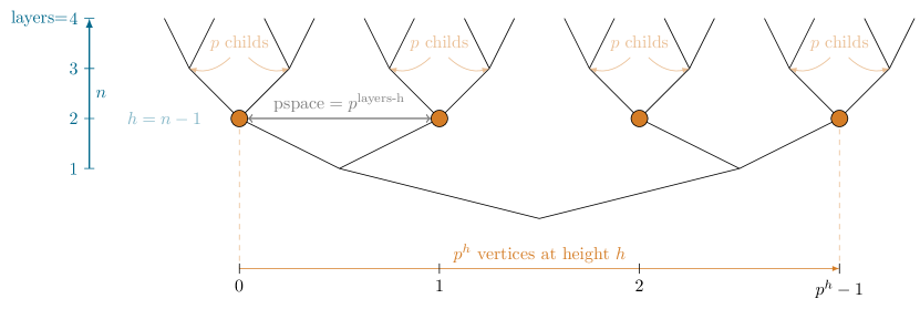
Figure 6: Ranges of the different loop variables for the first tree

Now fix $n\in\{1,\ldots,\text{layers}\}$, the loop starting at line $58$ goes over all the nodes at height ${\color[rgb]{0.4,0.6448,0.727}h}={\color[rgb]{0,.408,.545}n}-1$ and draws the edges between a node at height $n-1$ and its $q$ childs at height $n$. To do so, it fixes the horizontal position $k\in\{1,\ldots,p^{n-1}-1\}$ of the chosen node at height $n-1$. This node thus has to be shifted to the right by ${\color[rgb]{0.4167,0.245,0.075}pshift}={\color[rgb]{0.8334,0.49,0.15}k}*{\color[rgb]{0.5,0.5,0.5}\mathrm{pspace}}$ and hence drawn at the coordinates

$$({\color[rgb]{0.5,0.5,0.5}\mathrm{pspace}}-0.5+{\color[rgb]{0.8334,0.49,0.15}k}*{\color[rgb]{0.5,0.5,0.5}\mathrm{pspace}},0,n-1)=({\color[rgb]{0.5,0.5,0.5}\mathrm{pspace}}-0.5+{\color[rgb]{0.4167,0.245,0.075}pshift},0,n-1).$$

The childs are then located at height ${\color[rgb]{0,.408,.545}n}$. Similarly as above, the first child to be drawn has for horizontal coordinates the middle of $[0,q^{\mathrm{layers}-{\color[rgb]{0,.408,.545}n}-1}-1]$ and the “$\backslash\mathrm{child}$-th” is shifted to right by $\mathrm{child}*{\color[rgb]{0.5,0.5,0.5}\mathrm{pspace}}$. Hence the coordinates of the “$\backslash\mathrm{child}$-th” child is given by

$$({\color[rgb]{0.5,0.5,0.5}\mathrm{pspace}}/q-0.5+{\color[rgb]{0.4167,0.245,0.075}pshift}+\mathrm{child}*{\color[rgb]{0.5,0.5,0.5}\mathrm{pspace}},0,n-1).$$

Lines 79 to 116

This loop draws the brown tree on the plane $x=0$ and the Diestel-Leader graph at the same time.

Lines 79 to 95

The variable $k$ at line $79$ goes through the ${\color[rgb]{0.4,0.34,0.2}qrev}=q^{\mathrm{layers}-{\color[rgb]{0,.408,.545}n}}$ vertices at height $n$. Denote by $v$ the $k$-th vertex at this height. The loop for \child in 0,…,-1

goes through the $q$ childs of $v$ and draw the edge between $v$ and the $\backslash\mathrm{child}$-th child at height ${\color[rgb]{0,.408,.545}n}-1$. The coordinates of the nodes are computed in the same way as in the previous loop. (Remark that the heights in the current loop are swapped: the parent is at height $n$ and the childs are at height ${\color[rgb]{0,.408,.545}n}-1$ whereas in the previous one, the childs were at height ${\color[rgb]{0,.408,.545}n}$ and the parent at height ${\color[rgb]{0,.408,.545}n}-1$.) Inside the loop for \child in 0,…,-1 (starting line 81) lies also the part that draws the Diestel-Leader. Remember that $v$ is the current vertex at height ${\color[rgb]{0,.408,.545}n}$ in the $q$-regular tree $\mathbf{T}_{q}$. The loop for \kk in 0,…,-1 goes through all the vertices in the orange tree, drawn at height $n$. It will correspond to all the couple $(uv)$ such that $u\in\mathbf{T}_{p}$ is drawn at the same height (the $z$-coordinates) than $v$. To a given child $c$ of $v$ in $\mathbf{T}_{p}$, corresponds then the edge in the Diestel-Leader linking $(u,v)$ to $(u^{-},c)$, where we recall that $u^{-}$ is the unique predecesor of $u$ in $\mathbf{T}_{p}$ (see Section 1.1). Hence the point $(u,v)$ will be drawn at height $n$ and will have the same $x$-coordinates than $u$ and same $y$-coordinates than $v$, namely

$$\begin{cases}x&={\color[rgb]{0.5,0.5,0.5}\mathrm{pspace}}/(2p)-0.5+{\color[rgb]{0.4167,0.245,0.075}\mathrm{pshiftprime}}+childprime*{\color[rgb]{0.5,0.5,0.5}\mathrm{pspace}}/p,\\ y&=q^{n}/2-0.5+qshift,\\ z&=n\end{cases}$$

Similarly, the node $(u^{-},c)$ will be drawn at height $n-1$ and will have the same $x$-coordinates than $u^{-}$ and same $y$-coordinates than $c$, namely

$$\begin{cases}x&={\color[rgb]{0.5,0.5,0.5}\mathrm{pspace}}/2-0.5+{\color[rgb]{0.4167,0.245,0.075}\mathrm{pshiftprime}},\\ y&=q^{n}/2-0.5+\mathrm{qshift}+\mathrm{child}*q^{n}/q,\\ z&=n-1\end{cases}$$

2.2 The code

⬇

\documentclass[border=0mm]{standalone}

\usepackage[x11names]{xcolor}

\usepackage{tikz}

\usetikzlibrary{calc,math,backgrounds}

\usepackage{ifthen}

\usepackage{pgfplots}

\pgfplotsset{compat=1.18}

\definecolor{MFCB}{cmyk}{0,0.06,0.20,0.6}

\colorlet{Orange}{DarkOrange3!85}

\begin{document}

\begin{tikzpicture}\begin{axis}[

view={165}{10}, xlabel=$x$,

zlabel=$z$,

ylabel=$y$,

]

\tikzmath{

\p=2; \q=3;

\layers=3;for \nin {1,…,\layers}{\qrev=pow(\q,\layers-\n);\qn=pow(\q,\n);\pspace=pow(\p,\layers+1-\n); \pnm=pow(\p,\n-1);for \kin {0,…,\pnm-1}{\pshift=\k*\pspace;for \childin {0,…,\p-1}{{

\addplot3[Orange!20,thick] coordinates{(\pspace/(2*\p)-0.5+\pshift+\child*\pspace/\p,0,\n)

(\pspace/2-0.5+\pshift,0,\n-1)};

}; }; };for \kin {0,…,\qrev-1}{\qshift=\k*\qn;for \childin {0,…,\q-1}{{ \begin{scope}[on background layer]

\addplot3[MFCB!20,thick] coordinates{(0,\qn/2-0.5+\qshift,\n)

(0,\qn/(2*\q)-0.5+\qshift+\child*\qn/\q,\n-1)};

\end{scope}

};for \kkin {0,…,\pnm-1}{

\pshiftprime=\kk*\pspace;for \childprimein {0,…,\p-1}{{\addplot3[DeepSkyBlue4,thick] coordinates{(\pspace/(2*\p)-0.5+\pshiftprime+\childprime*\pspace/\p,

\qn/2-0.5+\qshift,\n)

(\pspace/2-0.5+\pshiftprime,\qn/(2*\q)-0.5+\qshift+\child*\qn/\q,\n-1)};

};};};}; };};}\end{axis}

\end{tikzpicture}

\end{document}

Acknowledgments We thank Tom Ferragut, Giles Gardam and Théo Laurent for their useful remarks and comments.

Fundings The athor is funded by the Deutsche Forschungsgemeinschaft (DFG, German Research Foundation) – Project-ID 427320536 – SFB 1442, as well as under Germany’s Excellence Strategy EXC 2044 –390685587, Mathematics Münster: Dynamics–Geometry– Structure. Amandine Escalier
Mathematisches Institut,
Fachbereich Mathematik und Informatik der Universität Münster,
Orléans-Ring 12,
48149 Münster,
Germany

References

- [DL01] R. Diestel and I. Leader. A conjecture concerning a limit of non-cayley graphs. Journal of Algebraic Combinatorics, 14:17–25, 2001.
- [EFW07] A Eskin, D Fisher, and K. Whyte. Quasi-isometries and rigidity of solvable groups. Pure and Applied Mathematics Quarterly, 3(4):927–947, 2007.
- [EFW12] A Eskin, D Fisher, and K. Whyte. Coarse differentiation of quasi-isometries i: Spaces not quasi-isometric to cayley graphs. Annals of Mathematics, 176(1):221–260, 2012.
- [Feu21] C. Feuersänger. Manual for package pgfplots, 2021. https://ctan.org/pkg/pgfplots.
- [Woe91] Wolfgang Woess. Topological groups and infinite graphs. Discrete Mathematics, 95(1):373–384, 1991.