First search for ultralight dark matter with a space-based gravitational-wave antenna: LISA Pathfinder

Abstract

We present here results from the first-ever search for dark photon dark matter that could have coupled to baryons in LISA Pathfinder, the technology demonstrator for a space-based gravitational-wave antenna. After analyzing approximately three months of data taken by LISA Pathfinder in the frequency range $[2\times 10^{-5},5]$ Hz, corresponding to dark photon masses of $[8\times 10^{-20},2\times 10^{-14}]$ eV/$c^{2}$, we find no evidence of a dark-matter signal, and set upper limits on the strength of the dark photon/baryon coupling. To perform this search, we leveraged methods that search for quasi-monochromatic gravitational-wave signals in ground-based interferometers, and are robust against non-Gaussianities and gaps in the data. Our work therefore represents a proof-of-concept test of search methods in LISA to find persistent, quasi-monochromatic signals, and shows our ability to handle non-Guassian artifacts and gaps while maintaining good sensitivity compared to the optimal matched filter. The results also indicate that these methods can be powerful tools in LISA to not only find dark matter, but also look for other persistent signals from e.g. intermediate-mass black hole inspirals and galactic white dwarf binaries.

I Introduction

LISA Pathfinder McNamara et al. (2008); Armano et al. (2009); Antonucci et al. (2012) was a demonstrator of some of the technologies to be used in LISA, the space-based gravitational-wave antenna to be launched in the second half of the next decade Danzmann and Team (2003); Amaro-Seoane et al. (2017). Its main goal, the demonstration that the noise in the separation of two test masses $\approx$ 40cm apart could be kept at a suitably low level to allow the detection of gravitational waves by LISA, was successfully achieved by LISA Pathfinder. In fact, LISA Pathfinder was a remarkable success and produced a noise power spectral density that surpassed the LPF mission requirement by more than an order of magnitude for some frequency regions and by a factor of a few compared to the LISA requirement Armano et al. (2016, 2018).

Though designed for the purpose described above, the data from LISA Pathfinder have been used in different ways to probe other areas of physics, such as quantifying possible noise correlations in future stochastic gravitational-wave background searches Boileau et al. (2022), measuring the value of Newton’s gravitational constant Armano et al. (2019a), testing the strong equivalence principle when spacecrafts orbit Lagrange points Congedo and De Marchi (2016), and bounding collapse models Carlesso et al. (2016). Such studies show that high-precision measurements of acceleration or displacement can be employed to tackle interesting physics problems for which the experiment was not primarily designed, and motivate the need for further analyses of LISA Pathfinder data lpf to see what other kinds of questions that this data, and the future LISA mission, can answer.

LISA Pathfinder data can be used to probe the existence of ultralight dark matter directly via its interactions with the test masses. Essentially, the instruments exists in a field or “wind” of dark matter, and this dark matter would couple to standard model particles in the test masses, causing sinusoidal oscillations of their positions over time at a frequency fixed by the dark matter mass. Scalar, dilaton dark matter would cause oscillations in the electron mass or other fundamental constants Stadnik and Flambaum (2015a, b, 2016), resulting in a change of the size of an object Grote and Stadnik (2019); axions Preskill et al. (1983) would alter the phase velocity of light Nagano et al. (2019, 2021), affecting the roundtrip time of laser light in LISA; dark photons could couple to baryons or baryon-lepton number in the test masses, leading to a sinusoidal force exerted on them Pierce et al. (2018). While the physics of each model is different, the observable is the same: time-varying positions or accelerations of test masses relative to one another.

The mass range to which space-based gravitational-wave detectors are sensitive is a function of the frequency range: $\mathcal{O}(10^{-5}-1)$ Hz corresponds to $\mathcal{O}(10^{-19}-10^{-14})$ eV/$c^{2}$. At such low masses – compared to those to which ground-based gravitational-wave detectors such as LIGO Aasi et al. (2015), Virgo (Acernese et al., 2015), and KAGRA Aso et al. (2013) could probe – the expected signal is monochromatic, since the frequency shift canonically introduced by the motion of the earth through the dark matter “wind” is very small compared to the frequency resolution of a search. Therefore, we cannot differentiate between a monochromatic and a “quasi”-monochromatic ultralight dark-matter signal at most frequencies to which LISA Pathfinder and LISA are sensitive.

There is a growing interest in using gravitational-wave detectors to search for ultralight dark matter. GEO600 data Dooley et al. (2016) was recently analyzed using a Logarithmic frequency axis Power Spectral Density (LPSD) method Tröbs and Heinzel (2006, 2009), yielding strong constraints on scalar, dilaton dark matter coupling to the beam splitter Vermeulen et al. (2021). Furthermore, constraints on vector dark matter, i.e. dark photons, were placed using data from the first Guo et al. (2019) and third Abbott et al. (2022) observing runs of advanced LIGO/Virgo/KAGRA that surpassed upper limits from the Eöt-Wash Schlamminger et al. (2008) and MICROSCOPE Bergé et al. (2018) experiments by a few orders of magnitude at frequencies between $\sim 100-1000$ Hz ($4\times 10^{-13}-4\times 10^{-12}$ eV/$c^{2}$). Finally, methods to search for axions and dilatons in different interferometer channels Nagano et al. (2019); Hall and Aggarwal (2022), for vector bosons with KAGRA Michimura et al. (2020), and tensor bosons Armaleo et al. (2021) in LIGO/Virgo/KAGRA and pulsar timing arrays Armaleo et al. (2020) have been developed for such kinds of searches.

What has not yet been done in this field of direct dark-matter searches with gravitational-wave detectors is to apply these methods to space-based instruments. While projected sensitivities have been estimated for a variety of dark-matter models Arvanitaki et al. (2015); Pierce et al. (2018); Morisaki et al. (2021), the development of algorithms tuned towards monochromatic signals in LISA, DECIGO Kawamura et al. (2021), and TianQin Luo et al. (2016) has not yet followed. In this work, we take a first step in this direction by performing a search of LISA Pathfinder data, a precursor to the kind of data that we expect in LISA, for ultralight dark matter, which requires that we develop methods to handle specific problems that LISA Pathfinder faced and LISA will face, such as non-Gaussianities, gaps, and sparse sampling at low frequencies Ferraioli et al. (2011); Edwards et al. (2020); Baghi et al. (2022) Specifically, we adapt methods developed in the context of quasi-monochromatic, persistent signals emitted by isolated neutron stars Riles (2017), planetary- and asteroid-mass primordial black hole binaries Miller et al. (2021a, 2022a); Guo and Miller (2022), depleting boson clouds around black holes D’Antonio et al. (2018); Isi et al. (2019), and dark matter that couples to ground-based gravitational-wave interferometers Pierce et al. (2018); Miller et al. (2021b), to look for dark matter in space with LISA Pathfinder.

The methods presented here are generically good at finding quasi-monochromatic signals in any dataset, regardless of the underlying physics Riles (2017); Sieniawska et al. (2019). They are also (1) robust against noise disturbances such as powerful lines, (2) efficiently deal with gaps in data collection, and (3) are computationally cheap compared to matched filtering, the optimal method to find weak signals buried in noise. In space-based detectors, gravitational waves from a variety of astrophysical sources, such as galactic white dwarf binaries or black hole inspirals Wyithe and Loeb (2003); Babak et al. (2017), will also be quasi-monochromatic and last for durations longer than the observing time Miller et al. (2021b, 2022b), or at least for greater lengths of time than in ground-based detectors, of $\mathcal{O}$(hours-days). Currently, proposals for parameter estimation and matched-filtering searches for gravitational waves with LISA struggle with each of the three aforementioned points Baghi et al. (2019); Dey et al. (2021); Blelly et al. (2021); therefore, the work presented here has much farther reaching implications than “just” a search for dark matter; it represents a comprehensive analysis scheme that can be applied to any quasi-monochromatic signal embedded in imperfect, non-Gaussian, gapped LISA data.

This paper is organized as follows: in section II, we describe the dark-matter signal expected at LISA Pathfinder when it flew; in section III, we explain which data segments from the $\sim 1.5$ year run we analyze. Section IV focuses on the methods that we use to search for ultralight dark matter, one that breaks the data into smaller, Gaussian chunks, and another that match filters the data with a signal model coherently. We present our results in section V, which include rejecting strong outliers in the data and upper limits on the strength of the coupling of dark matter to baryons. Finally, we draw some conclusions in section VI and discuss opportunities for future work.

II Dark matter signal

Dark matter could be composed of spin-1 particles, which we denote as dark photons. The relic abundance of dark matter can be explained entirely by dark photons, which could arise from the misalignment mechanism Nelson and Scholtz (2011); Arias et al. (2012); Graham et al. (2016), parametric resonance or the tachyonic instability of a scalar field Agrawal et al. (2020); Co et al. (2019); Bastero-Gil et al. (2019); Dror et al. (2019), or from cosmic string network decays Long and Wang (2019). Dark photons could couple directly to baryon or baryon-lepton number in the two LISA Pathfinder test masses, and exert a “dark” force on the them, causing quasi-sinusoidal oscillations Pierce et al. (2018); Miller et al. (2021b).

Similarly to the ordinary photon, the vector potential for a single dark photon particle can be written as:

$$\vec{A}(t,\vec{x})=\left(\frac{\hbar\sqrt{2\rho_{\text{DM}}}}{mc^{2}}\frac{1}{\sqrt{\epsilon_{0}}}\right)\sin\left(\omega t-\vec{k}\cdot\vec{x}+\phi\right),$$ (1)

where $\omega=(mc^{2})/\hbar$ is the angular Compton frequency, $\vec{k}=(m\vec{v}_{\text{obs}})/\hbar$ is the wave vector, $m$ is the mass of the vector field, $\epsilon_{0}$ is the permittivity of free space and $\phi$ is a random phase.

The Lagrangian $\mathcal{L}$ that characterizes the dark photon coupling to a number current density $J^{\mu}$ of baryons or baryons minus leptons is:

$$\mathcal{L}=-\frac{1}{4\mu_{0}}F^{\mu\nu}F_{\mu\nu}+\frac{1}{2\mu_{0}}\left(\frac{mc}{\hbar}\right)^{2}A^{\mu}A_{\mu}-\epsilon eJ^{\mu}A_{\mu},\\$$ (2)

where $F_{\mu\nu}$ indicates the dark electromagnetic field tensor, $\mu_{0}$ is the magnetic permeability in vacuum, $A_{\mu}$ is the four-vector potential of the dark photon, $e$ is the electric charge, and $\epsilon$ is the strength of the particle/dark photon coupling normalized by the electromagnetic coupling constant.

Dark photons would cause small motions in each of the test masses, and lead to an observable effect because the test masses are separated from each other and hence experience slightly different dark photon dark matter phases. Such a phase difference leads to a change of the arm length over time. What is needed, therefore, is very precise measurements of the positions of the two test masses, something which LISA Pathfinder provides.

Each test mass experiences an almost identical acceleration:

$$\vec{a}(t,\vec{x})\simeq\epsilon e\frac{q}{M}\omega\vec{A}\cos(\omega t-\vec{k}\cdot\vec{x}+\phi),$$ (3)

where $q/M$ is the charge-to-mass ratio of the test masses. This effect is in fact a residual one: if the test masses were made of different materials, then the signal induced from dark photons coupling to baryon-lepton number would be enhanced Michimura et al. (2020). A simple relation between dark photon parameters and the effective strain $h_{D}$ experienced by LISA Pathfinder can be written as Pierce et al. (2018); Morisaki et al. (2021); Abbott et al. (2022):

$$\sqrt{\left\langle h_{D}^{2}\right\rangle} = C_{\rm LPF}\frac{q}{M}\frac{v_{0}}{2\pi c^{2}}\sqrt{\frac{2\rho_{\mathrm{DM}}}{\epsilon_{0}}}\frac{e\epsilon}{f_{A}},$$ (4)

where $f_{A}=\omega/(2\pi)$ is the frequency of the dark-matter particle, and $C_{\rm LPF}=1/3$ is a geometrical factor obtained by averaging the acceleration over all possible dark photon propagation and polarization directions for a single arm, using the appendix in Pierce et al. (2018) to aid with this calculation. We note $C_{\rm LPF}$ is a factor of $\sqrt{2}$ smaller than the geometrical factor in LIGO $C_{\rm LIGO}=\sqrt{2}/3$, which indicates that an L-shaped interferometer would observe a signal $\sqrt{2}\sim 1.4$ times stronger than a single arm would.

As we can see from equation 3, the test masses will experience a sinusoidal oscillation of their positions over time, at a frequency set by the mass of the dark-matter particle. However, if we observe for longer than the dark-matter signal coherence time $T_{\text{coh}}$, then we will resolve stochastic frequency fluctuations $\Delta f$ about the dark-matter mass, induced by the motion of the spacecraft relative to the dark-matter field. In other words, we wish to contain these fluctuations to one frequency bin $\delta f$, so we require:

$$\Delta f=\frac{1}{2}\left(\frac{v_{0}}{c}\right)^{2}f_{A}<\delta f=\frac{1}{T_{\text{FFT}}}$$ (5)

which leads to:

$$T_{\text{FFT}}<10^{7}\text{ s}\left(\frac{0.1\text{ Hz}}{f_{A}}\right)\sim T_{\text{coh}}$$ (6)

where $T_{\text{FFT}}$ is the fast Fourier transform length, and $v_{0}\simeq 220$ km/s is the velocity at which dark matter orbits the center of our galaxy, i.e. the virial velocity Smith et al. (2007). Here, we observe for a duration much less than $T_{\text{coh}}$, which implies that the signal will be fully contained within one frequency bin, i.e. it is purely monochromatic for our purposes.

III Data

We analyze eight periods of differential acceleration time-series LISA Pathfinder data, whose details are given in table 1, each of which lasts from $\sim 5$ days to $\sim 2.5$ weeks lpf . One segment, #6, that began on 14 February 2017, was obtained at a much lower temperature than the others, which resulted in a different noise level Armano et al. (2018). We therefore treat it as a separate dataset from the others, as will be detailed in Sec. IV, and present all constraints based on this dataset.

In table 1, we also report the $T_{\text{FFT}}$ such that the data within that segment remain Gaussian at the 5% significance level, based on the Kolmogorov-Smirnov test Massey Jr (1951). We see here that some segments remain Gaussian for longer compared to others, but in general, the duration of Gaussian data is short compared to the segment duration. Therefore, for the semi-coherent search, we consider $T_{\text{FFT}}=8192$ s for all segments, as explained in the next section.

number	date	duration (days)	$T_{\rm FFT}$ (s)	Temp (C)
1	2016-03-$21$	5.08	16384	22
2	2016-04-$04$	9.33	16384	22
3	2016-07-$24$	5.29	4096	22
4	2016-11-$16$	9.82	8192	22
5	2016-12-$26$	17.86	8192	22
6	2017-02-$14$	13.33	8192	11
7	2017-05-$29$	7.04	131072	22
8	2017-06-$08$	8.4	262144	22

Table 1: Data segments considered in this search obtained from lpf . Segment # 6 is treated as a separate dataset here: we perform coincidences of the other seven datasets with segment # 6 in order to reduce the number of outliers.

IV Method

.

IV.1 Semi-coherent method: projection

Due to the non-Gaussian nature of the noise when observing for longer than $\sim 8192$ s, we break the dataset into smaller chunks, of duration $T_{\text{FFT}}=8192$ s, analyze these chunks coherently, and then combine their power incoherently, that is, without the phase information. To perform this analysis, we leverage existing methods used in continuous-wave data analysis for the search of depleting boson clouds around black holes D’Antonio et al. (2018), and for dark matter that could couple to ground-based gravitational-wave detectors Miller et al. (2021b).

IV.1.1 Creation of time/frequency peakmaps

This semi-coherent method Miller et al. (2021b) operates on data in the time/frequency plane, so we take fast Fourier Transforms with $T_{\text{FFT}}=8192$ s, divide the square modulus of the fast Fourier transform by a running-median estimation of the power spectral density to obtain “equalized power” (whose mean value in noise should be 1), set a threshold $\theta_{\rm thr}=2.5$ to remove spurious noise peaks, and select local maxima in the power spectra. Each of these choices is motivated in Astone et al. (2005), and is meant to be robust against the presence of non-stationarities in the noise. This threshold in fact comes from empirical studies in Astone et al. (2005) showing that while the ideal threshold in Gaussian noise is 2, a threshold of 2.5 allows for a higher value of the detection statistic, and a reduction in the number of outliers in the presence of disturbances in real LIGO/Virgo data. The “local maxima” criteria is applied because spectral disturbances in real data may not be well localized to one frequency bin (i.e. they have finite coherence times that do not match the $T_{\text{FFT}}$ chosen), or they may turn on and off over the course of the run (or even within one $T_{\text{FFT}}$. Therefore, selecting local maxima helps to minimize contamination of nearby bins from noise lines. The thresholded time/frequency maps are called “peakmaps”, in which only powerful “peaks”, i.e. points in the time/frequency plane, remain after the thresholding and local maxima selection.

This procedure results in the left-hand panel of figure 1, for segment #6. We employ the semi-coherent method at frequencies above $\sim 1$ mHz, since below this value, it becomes difficult to estimate the power spectral density using a simple running median, due to the lack of data points at such low frequencies.

IV.1.2 Projection and selection of candidates

After we have created the time/frequency peakmaps, we then attempt to recover some signal power that has been lost due to dividing the data into chunks. To do this, we integrate the peakmap over time, i.e. we project it onto the frequency axis, summing only whether or not a peak appears at a given time and frequency, not the equalized power that is given in the color bar of the left-hand panel of figure 1. This is a choice that is, again, motivated by the presence of noise artifacts: in pure Gaussian noise, summing signal power provides the best chances of detection. However, there are powerful noise lines, e.g. the one at 1 Hz, that we do not want to blind us to possible signals. In this way, we reduce the signal-to-noise ratio of the instrumental lines, while preserving sensitivity towards weak, monochromatic signals. We sum each peakmap from datasets 1-5; 7-8 together in this method, allowing us to recover some signal-to-noise ratio that is lost by breaking the data into chunks of length $T_{\text{FFT}}$.

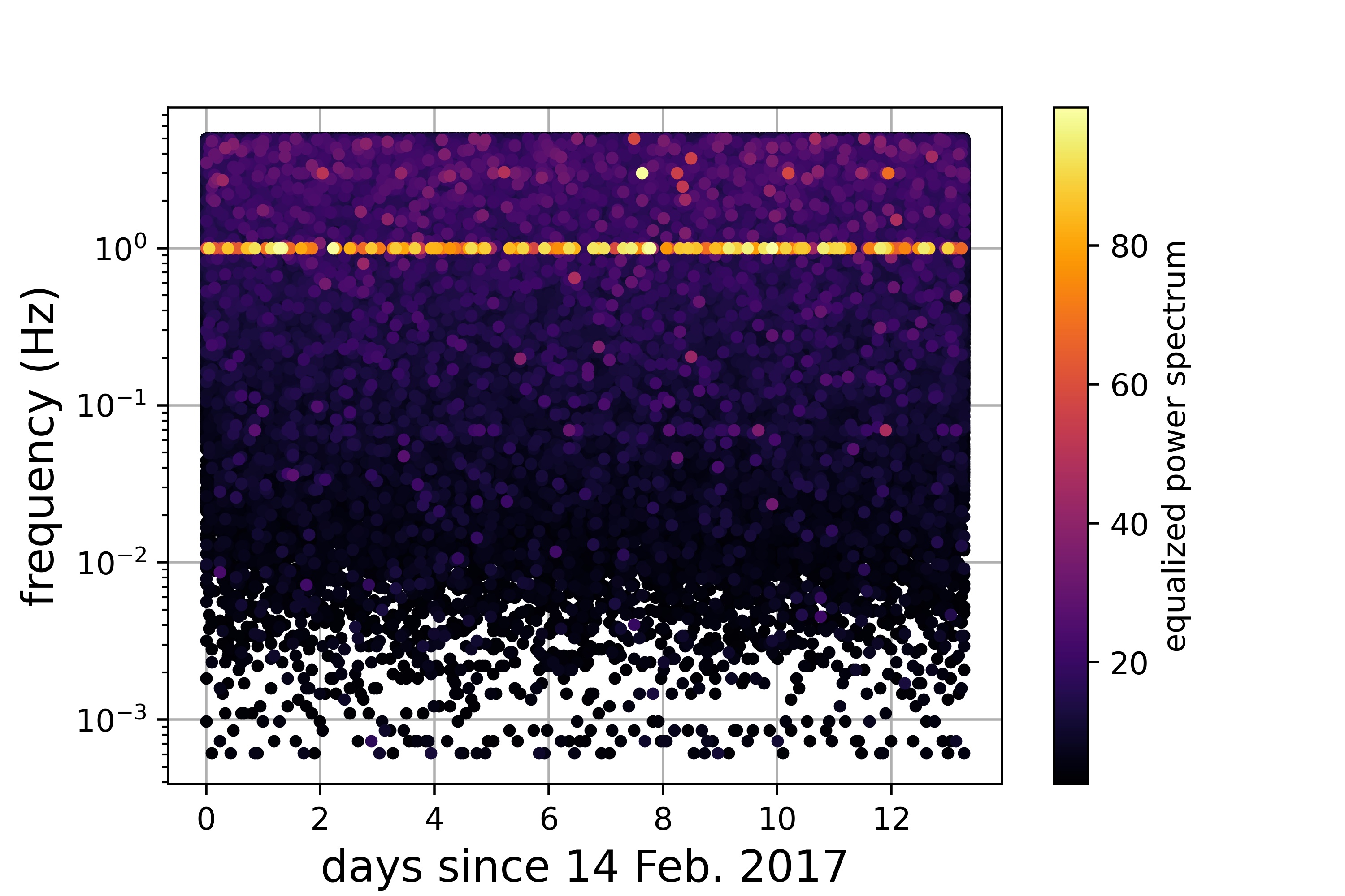
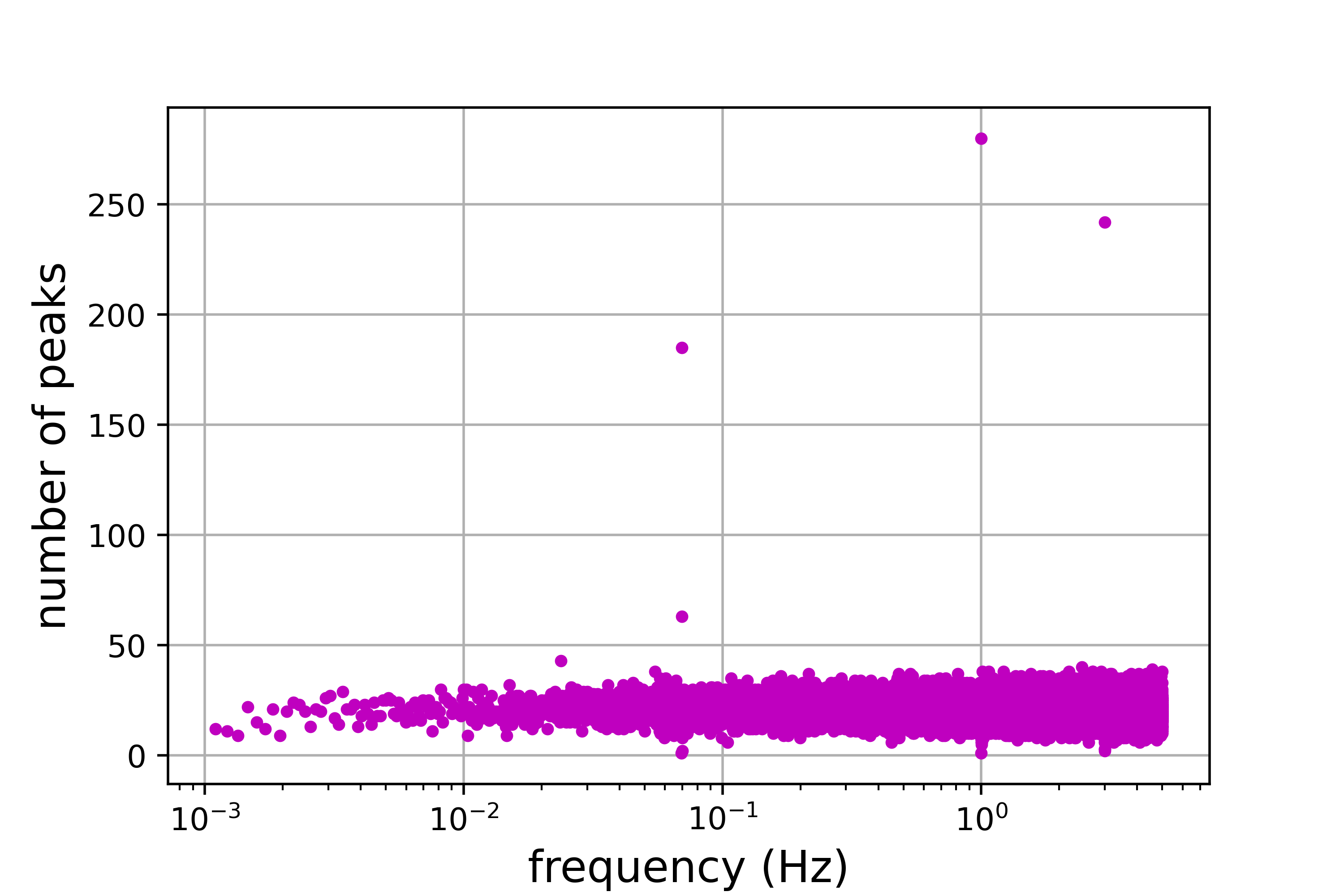
Figure 1: Left: example time/frequency peakmap used in the semi-coherent search. Right: projection of the peakmap onto the frequency axis, corresponding to an integration over time.

At this point, we obtain a “histogram” of the number of peaks at a given frequency, in the right-hand panel of figure 1. It is on this projected peakmap that we select possible significant candidates, i.e. particular frequencies, whose number counts are high relative to other frequencies. Since the frequency range spans three orders of magnitude, we select candidates uniformly in the log of frequency. We decide on a certain number of candidates $N_{\rm cand}$ to select such that we would expect a certain number of coincidences $N_{\rm coin}$ between the combined dataset (segments #1-5; 7-8) and segment #6 if the data were purely Gaussian in the frequency band of width $B$:

$$N_{\rm cand}\approx\sqrt{N_{\rm coin}T_{\text{FFT}}B}.$$ (7)

Here, we set $N_{\rm coin}=1$, $B$ = 5 Hz, and $T_{\text{FFT}}=8192$ s, so we select $N_{\rm cand}\approx 200$ candidates uniformly in logarithmic frequency. We select the strongest candidate in each sub-band.

Once we have these candidates, we compute our detection statistic, the critical ratio (CR):

$$CR=\frac{n-\mu}{\sigma},$$ (8)

where $n$ is the number of peaks at a given frequency, and $\mu$ and $\sigma$ are the average number and standard deviation of peaks across the sub-band, respectively. The CR is a random variable with mean 0 and standard devitation of 1; therefore, we set a threshold $CR_{\rm thr}=5$, corresponding to 5 standard deviations from the mean, that indicates that a particular candidate is “significant” and needs to be studied further.

IV.2 Fully-coherent method: matched-filter

For the frequencies considered in this analysis, and for the durations analyzed (see table 1), equation 6 indicates that the signal will be purely monochromatic; hence, we also perform a fully coherent search of each segment, by simply taking a fast Fourier Transform and computing the so-called matched filter signal-to-noise ratio (SNR) $\rho$:

$$\rho^{2} = 4\text{ Re}\left[\int_{0}^{\infty}df\frac{\tilde{h}(f)\tilde{d}(f)}{S_{n}(f)}\right]$$ (9)

$$= 4\text{ Re}\left[\frac{\tilde{d}(f)^{2}}{S_{n}(f)}\right]$$ (10)

where the tilde denotes the Fourier Transform of the corresponding quantity, $\tilde{d}(f)$ is the Fourier transform of the time-series $\Delta g$ acceleration data $d(t)$, $\tilde{h}(f)$ is the Fourier Transform of the waveform for the dark-photon signal $h(t)$, and $S_{n}$ is the power spectral density of the noise. To pass from the first to the second line in the above equation, we note that our desired signal is purely monochromatic. Therefore, the best filter, at each frequency, is simply a monochromatic signal at that frequency, and the number of templates used is simply equal to the number of frequencies analyzed, $N_{f}\sim 3.4\times 10^{6}$. We impose a threshold $\rho_{\rm thr}=8$ to indicate “significant” events, which corresponds to a false alarm probability, in pure Gaussian noise accounting for the trials factor, of 1 per $10^{9}$.

IV.2.1 PSD estimation at low frequencies

The sparseness of LISA Pathfinder data at low frequencies (defined here as less than 1 mHz) is problematic for a running-median estimation of the PSD. Hence, we employ a method developed in Castelli (2020) in order to obtain a robust low-frequency estimation of the PSD. The concept is to average Black-Harris windowed, 50% interlaced power spectra, obtained with a fixed $T_{\text{FFT}}$ at a given frequency, and then subsequently decrease $T_{\text{FFT}}$ at higher frequencies, resulting in more spectra to average. The frequencies $f_{j}$ at which the PSD estimation are performed are given by a recursive formula:

$$f_{j} = \frac{2}{(3/5)^{j-1}}f_{0}$$ (11)

$$f_{0} = \frac{M}{N_{\rm max}\Delta T}$$ (12)

where $M$ is the spacing between frequency bins needed to avoid spectral leakage from the averaging window among neighboring frequencies, $N_{\rm max}$ is the maximum number of samples to fast Fourier transform (for the starting $T_{\text{FFT}}=T_{0}=2\times 10^{5}$ s), and $\Delta T=1/10$ s is the sampling time. Here, $N_{\rm max}=\frac{T_{0}}{\Delta T}=2\times 10^{6}$ samples, and $M$ is set to 4 bins at $f_{0}$, and 8 bins for all others, obtained by ensuring a lack of correlation between neighboring bins Vitale et al. (2014). The factor $3/5$ is obtained by avoiding correlations between two neighboring frequency bins:

$$\frac{M-\alpha}{M+\alpha}=\frac{3}{5},$$ (13)

where $\alpha=2$ ensures that no correlations in the PSD exist between frequencies spaced by with a spacing $\delta f=\frac{2\alpha}{T_{\text{FFT}}}$.

$T_{\text{FFT}}$ scales with the same relation as:

$$T_{\text{FFT},j}=\left(\frac{3}{5}\right)^{j-1}N_{\rm max}\Delta T$$ (14)

By windowing, Fourier transforming and averaging the data in chunks of length $T_{\text{FFT},j}$, we obtain the values of the PSD at frequencies between $20\mu$Hz and $\sim 1$mHz, shown in figure 2 as black dots. For the rest of the parameter space, a running median estimation over 20 bins is employed to estimate the PSD, as in many LIGO/Virgo/KAGRA searches.

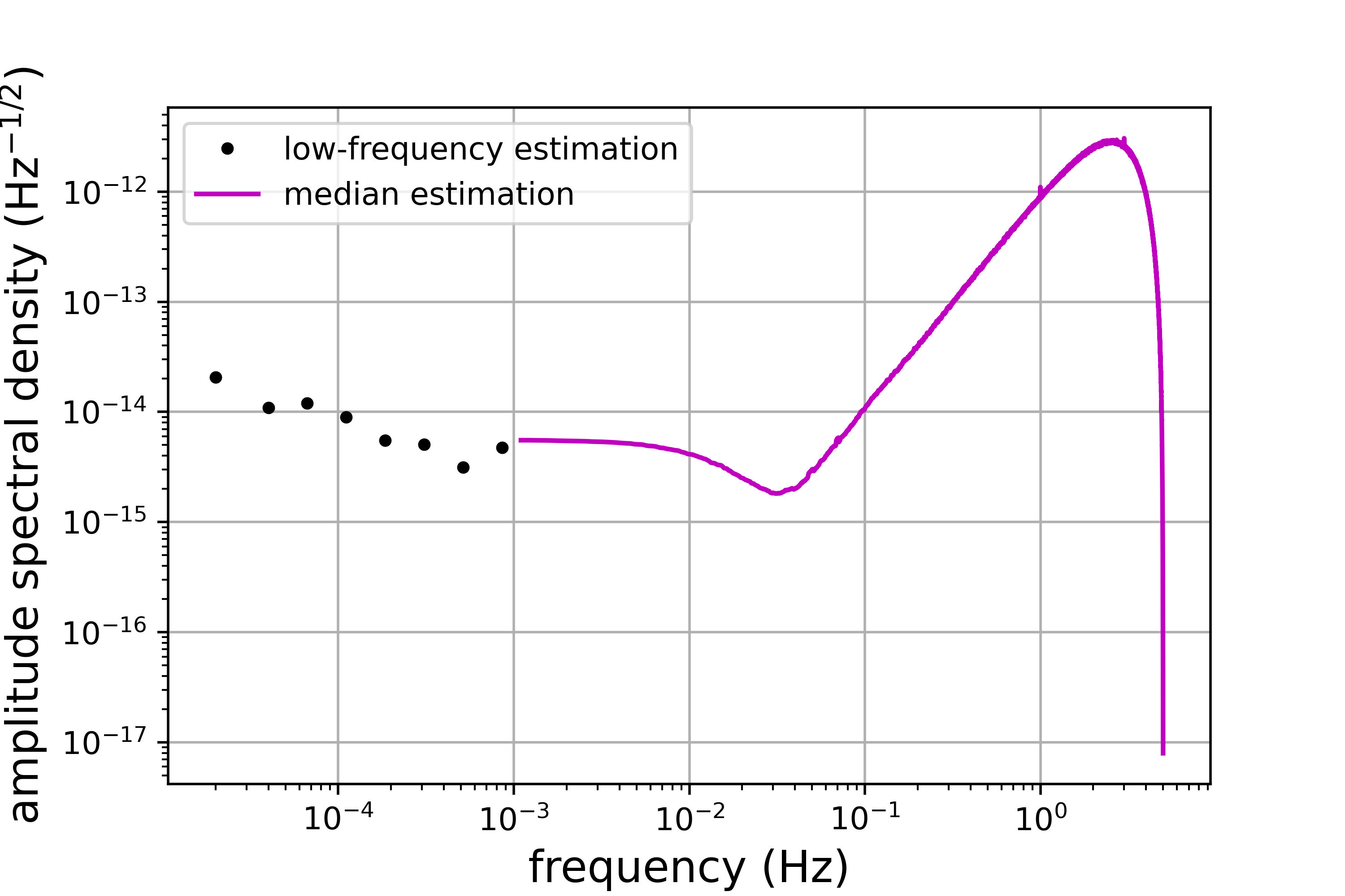
Figure 2: Estimation of the amplitude spectral density at low and high frequencies, using the method described in Castelli (2020) and a running median, respectively.

IV.3 Coincidences

We have indicated in table 1 eight segments that have been analyzed in this work. However, we only have data from one detector. Typically, in gravitational-wave data analysis, we look for similar signals in a collection of detectors to rule out the possibility of false alarms. In this case, though, we can look for coincidences between two datasets if their noise distributions are sufficiently different, such that they “function” as independent probes of dark matter. Furthermore, the dark-matter signal should always be present in the data; therefore, if a candidate is seen in one segment but not in another, this would indicate that it is due to something artificial, not astrophysical.

In the semi-coherent case, we sum the peakmaps from segments $\#1-5;7-8$ and require that a candidate in one detector appear within 2 frequency bins of a candidate in another. This choice of 2 bins is in fact very generous: the dark-matter signal should be exactly at the same frequency in each segment. We then impose a threshold on the critical ratio, requiring that a candidate’s CR is greater than $CR_{\rm thr}=5$.

In the fully-coherent searches, we do coincidences between each segment and segment $\#6$, and again require that candidates be within 2 frequency bins of each other. In this case, however, the size of the frequency bins of each segment will be slightly different, since their durations are not equal. We therefore use the larger of the two frequency bins to determine whether a coincidence has occurred. Then, we impose that the SNR must be greater than $\rho_{\rm thr}=8$. As a last stringent check, we will also require that a candidate be present in each data segment for it to be considered as an “outlier” worthy of further study.

V Results

We present here the results of our search for dark matter interacting with the test masses in LISA Pathfinder.

In the semi-coherent search in the high-frequency regime, the only coincident outliers above $CR_{\rm thr}$ were at $\sim 70$ mHz, 1 Hz and 3 Hz. These frequencies are contaminated with very strong noise lines and can thus be discarded. At 70 mHz, there is a known noise disturbacne due to the thrusters Armano et al. (2019b); at 1 Hz and 3 Hz, these are harmonics arising from electrical cross-couplings from the pulse-per-second timing signal present on the spacecraft Armano et al. (2022).

In the fully-coherent search, across all frequencies, we only obtained three coincident outliers in at least two of the segments analyzed that were not due to a particular known noise disturbance. They are given in table 2, and are barely above the SNR threshold set. We note, however, that these outliers did not appear in each segment that we separately analyzed, indicating that they are due to noise disturbances.

frequency (Hz)	SNR
0.474766	8.57
1.213422	8.50
2.584182	8.26

Table 2: Remaining candidates from the fully coherent, high-frequency search that appeared in at least two the datasets analyzed. We note that these candidates did not appear in all segments analyzed, as we would expect for a true dark photon signal; thus, we veto them.

For the critical ratio and the matched-filter SNR, we provide the statistical distributions obtained from the search in figures 3 and 4, respectively. We can see here that these distributions are not exactly Gaussian, due to the presence of non-stationarities in the data.

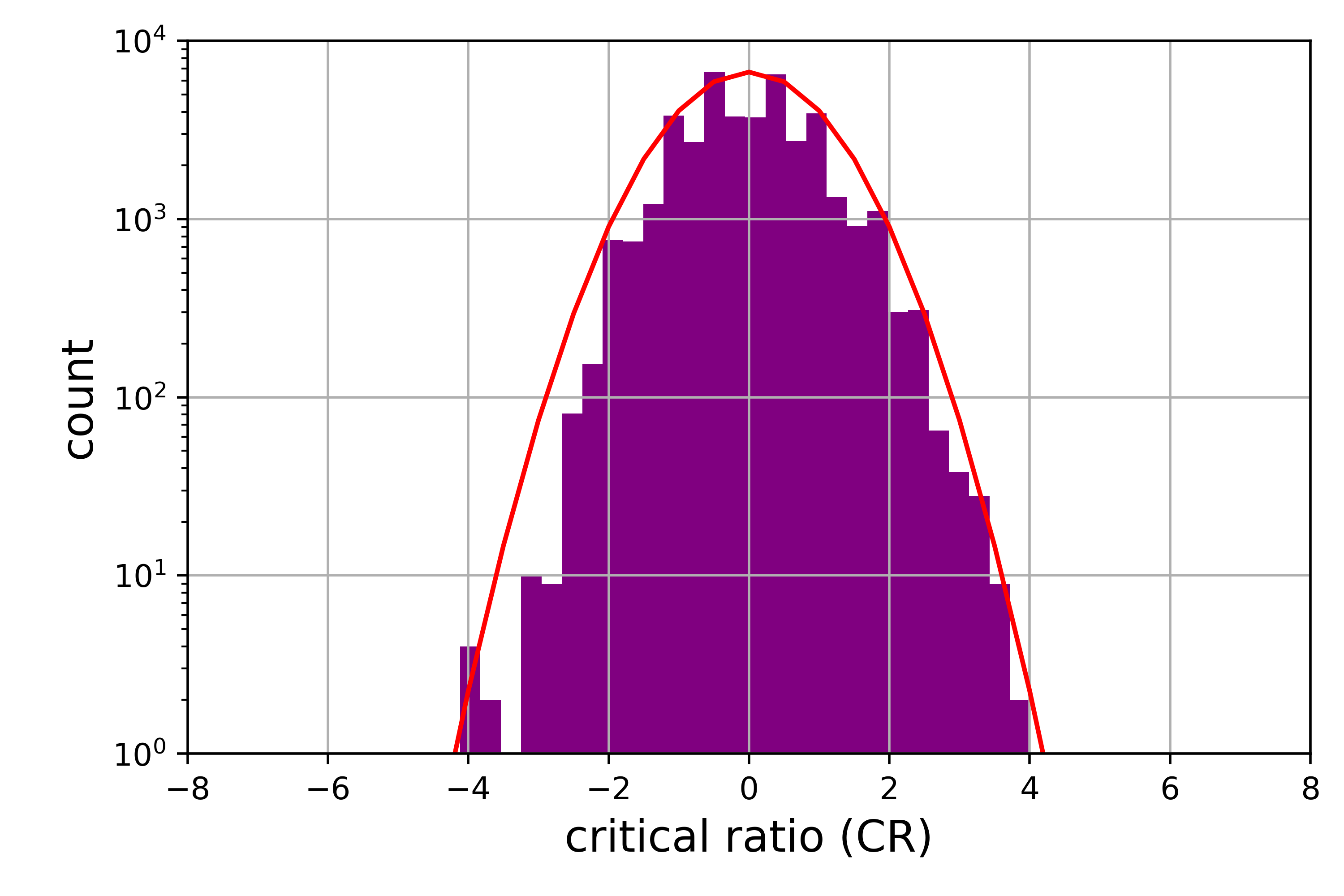
Figure 3: Distribution of the semi-coherent detection statistic $CR$, with a Gaussian curve overlayed for data segment #6 starting on 14 Feb. 2017.

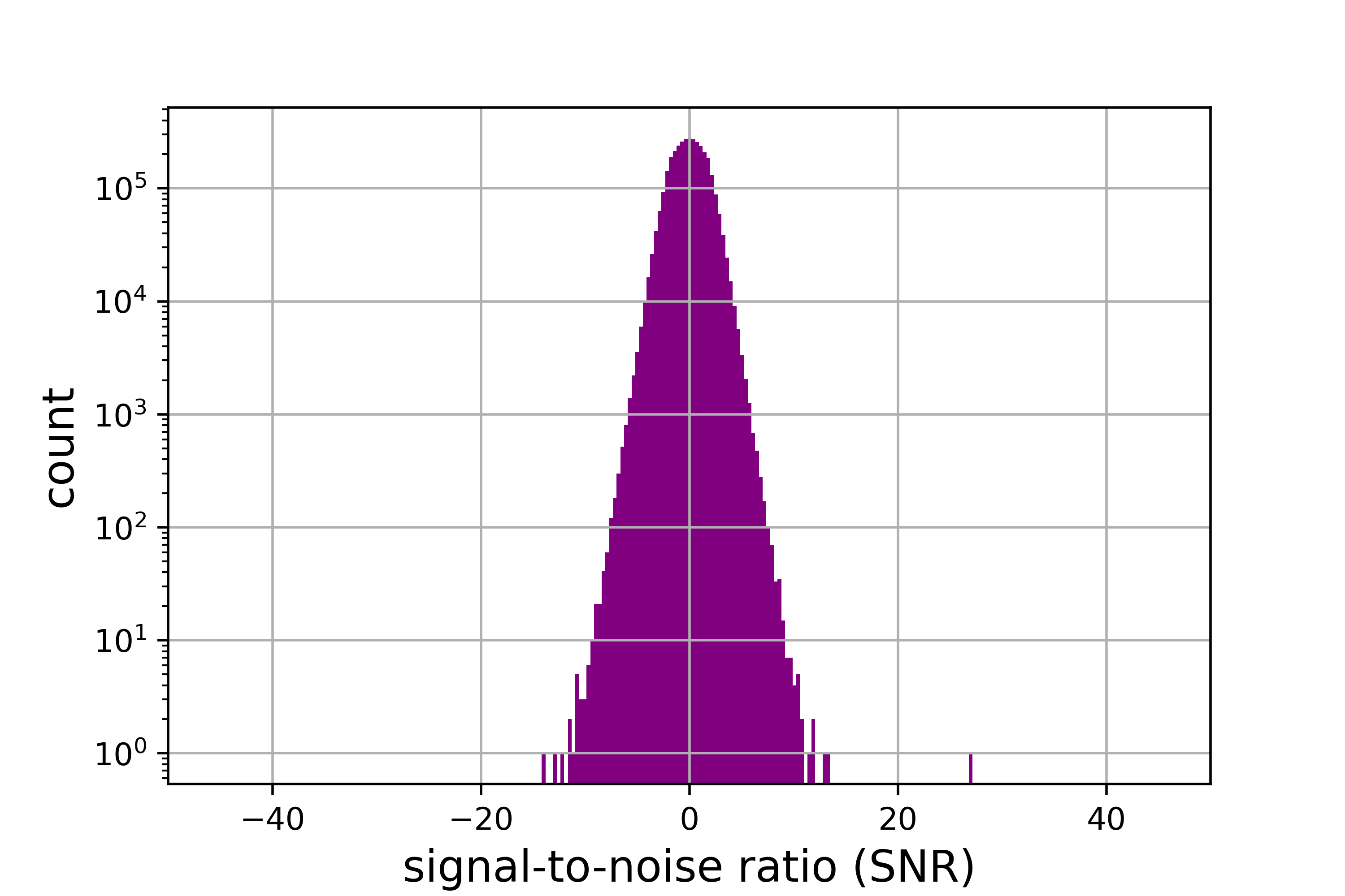
Figure 4: Distribution of the matched-filter detection statistic $\rho$ across the whole frequency range, for data segment #6 starting on 14 Feb 2017.

After vetoing all candidates, we then set upper limits on the coupling of dark matter to baryons in the test masses. We provide these limits in figure 5 in the low- and high-frequency regime. Specifically, in the high-frequency regime, we calculate these limits with both the results of the projection method and the matched filter for comparison. To obtain these limits, we employ the Feldman-Cousins approach Feldman and Cousins (1998) to map values of the critical ratio and SNR to “inferred” ones to ensure complete coverage at the chosen confidence level (95% in this case) using table 10 of Feldman and Cousins (1998). This procedure inherently assumes that the critical ratio and SNR follow Gaussian distributions, but is robust against non-Gaussianities: it provides conservative results with respect to simulations of dark-photon signals injected in real data (see figure 12 in Miller et al. (2021b)). From these “inferred” values of our detection statistics, we compute the constraint on the coupling strength using equation 30 in Miller et al. (2021b), and equation 4 here. Equation 30 in Miller et al. (2021b) arises from theoretically calculating the minimum detectable amplitude of a monochromatic signal that our search could see in Gaussian noise.

We note that the upper limits for the semi-coherent method, which combine the peaks in each segment, are shown for the “limiting” segment #6, since the duration and noise spectral density of this segment impede the sensitivity of the semi-coherent search relative to the other segments. If we were, instead, to use the critical ratios arising from integrating over each of the other segments, the limits would be lower by $\sim 2$, representing the ratio between the total observation time of segments #1-5; 7-8, and segment #6.

There is an additional effect that must be accounted for when calculating these upper limits. Due to the fact that $T_{\text{obs}}<<T_{\text{coh}}$ for the parameter space considered here, the stochastic nature of the signal amplitude affects the strength of the dark-matter coupling that we could observe. In other words, it could be possible that we would observe the dark-matter field amplitude at a near-zero value, something that does not happen in the regime $T_{\text{obs}}>>T_{\text{coh}}$, since we break the data into chunks of length $T_{\text{FFT}}\sim T_{\text{coh}}$, i.e. we observe for a full coherence time. These effects have been calculated for both scalar, axion dark matter Centers et al. (2021) and vector dark matter (dark photons) Nakatsuka et al. (2022). This stochastic effect amounts to an $\mathcal{O}(1)$ loosening of the upper limits in amplitude, and in our case, our limits on $\epsilon^{2}$ must be increased by a factor of 9. This correction has been applied in figure 5.

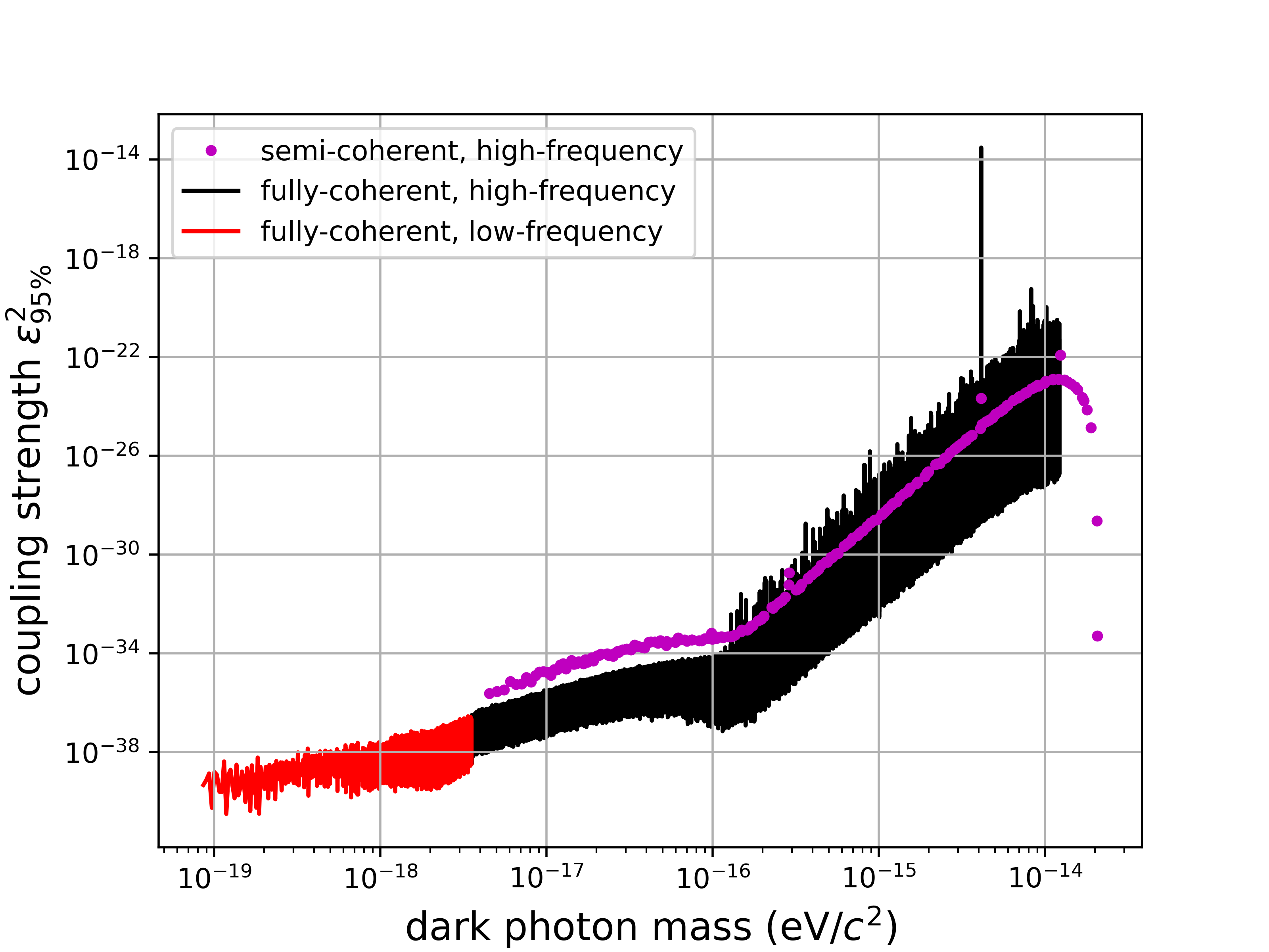
Figure 5: Upper limits in both the fully-coherent and semi-coherent regimes, with the red indicating the regime in which the low-frequency PSD estimation was used, for the period starting 14 Feb. 2017. The mass range shown on the $x$-axis corresponds to the frequency range $[2\times 10^{-5},5]$ Hz.

VI Conclusions

We have performed the first search for dark photon dark matter with LISA Pathfinder data, and have set upper limits on the coupling of dark photons to baryons in the test masses used in this mission. While these limits are not stringent compared to those from torsion balance experiments Schlamminger et al. (2008); Bergé et al. (2018), the work here provides a proof-of-concept pipeline to analyze future LISA data and perform dark-matter searches. Interestingly, we had to consider problems such as PSD estimation at very low frequencies, performing coincidences using one instrument, dealing with non-Gaussian artifacts arising from a gravitational-wave detector in space, and breaking the search into semi-coherent and fully-coherent regimes. Even though there were not many visible (by eye) non-Gaussian disturbances, the Gaussianity of this data broke down after $\mathcal{O}(\rm hours-days)$ in each segment analyzed. Our work therefore motivates the development of more advanced PSD estimation algorithms that can handle future data in LISA, the need for semi-coherent, time/frequency-based analyses of the data, and the power that search techniques designed for quasi-monochromatic signals in ground-based gravitational-wave detectors have when applied to a LISA-like mission.

Furthermore, in LISA, many astrophysical signals will be almost monochromatic – light binary black hole inspirals, inspiraling galactic white dwarf binaries, etc.–; therefore, our work shows how effective time/frequency analyses, as opposed to pure, computationally expensive matched filters, can be to look for different kinds of signals in future LISA data. While there is of course a sacrifice in sensitivity, evidenced by comparing the purple and magenta curves in the right-hand panel of figure 5, the difference is, at most, an order of magnitude in $\epsilon^{2}$ at $\sim 1$ mHz, meaning a factor of a few in strain, which is consistent with the comparison of semi-coherent methods to matched filtering given in Astone et al. (2014).

For dark-matter searches, LISA will provide access to masses that ground-based gravitational-wave detectors simply cannot probe, due to seismic activity and Newtonian noise on earth. The sensitivity achievable in LISA is expected to surpass by several orders of magnitude the existing constraints on $\epsilon^{2}$ from torsion-balance experiments Pierce et al. (2018). It is therefore worth investing in data-analysis pipelines in LISA, such as the one employed here, to perform searches to potentially directly detect dark matter, and also other astrophysical sources that would emit quasi-monochromatic signals.

Future work will include implementing a more robust estimation of the background of our detection statistics as described in Tenorio et al. (2022), extending our analysis to the whole LISA Pathfinder dataset, performing simulations of dark-matter particles interacting with the detector, and applying this analysis to other types of dark-matter that could be detected, e.g. the dark photon arising from kinetic mixing that couples to the ordinary photon Chaudhuri et al. (2015). All of these avenues of research will be relevant for when LISA eventually flies.

References

- McNamara et al. (2008) P. McNamara, S. Vitale, and K. Danzmann (LISA), Class. Quant. Grav. 25, 114034 (2008).
- Armano et al. (2009) M. Armano et al., Class. Quant. Grav. 26, 094001 (2009).
- Antonucci et al. (2012) F. Antonucci et al., Class. Quant. Grav. 29, 124014 (2012).
- Danzmann and Team (2003) K. Danzmann and L. S. Team, Advances in Space Research 32, 1233 (2003).
- Amaro-Seoane et al. (2017) P. Amaro-Seoane et al. (LISA), (2017), arXiv:1702.00786 [astro-ph.IM] .
- Armano et al. (2016) M. Armano et al., Phys. Rev. Lett. 116, 231101 (2016).
- Armano et al. (2018) M. Armano et al., Phys. Rev. Lett. 120, 061101 (2018).
- Boileau et al. (2022) G. Boileau, N. Christensen, and R. Meyer, Phys. Rev. D 106, 063025 (2022), arXiv:2204.03867 [gr-qc] .
- Armano et al. (2019a) M. Armano et al. (LISA Pathfinder), Phys. Rev. D 100, 062003 (2019a).
- Congedo and De Marchi (2016) G. Congedo and F. De Marchi, Phys. Rev. D 93, 102003 (2016), arXiv:1602.05949 [gr-qc] .
- Carlesso et al. (2016) M. Carlesso, A. Bassi, P. Falferi, and A. Vinante, Phys. Rev. D 94, 124036 (2016), arXiv:1606.04581 [quant-ph] .
- (12) “LISA Pathfinder Legacy Archive,” http://lpf.esac.esa.int/lpfsa/.
- Stadnik and Flambaum (2015a) Y. Stadnik and V. Flambaum, Physical Review Letters 114, 161301 (2015a).
- Stadnik and Flambaum (2015b) Y. Stadnik and V. Flambaum, Physical Review Letters 115, 201301 (2015b).
- Stadnik and Flambaum (2016) Y. Stadnik and V. Flambaum, Physical Review A 93, 063630 (2016).
- Grote and Stadnik (2019) H. Grote and Y. Stadnik, Physical Review Research 1, 033187 (2019).
- Preskill et al. (1983) J. Preskill, M. B. Wise, and F. Wilczek, Phys. Lett. B 120, 127 (1983).
- Nagano et al. (2019) K. Nagano, T. Fujita, Y. Michimura, and I. Obata, Physical Review Letters 123, 111301 (2019).
- Nagano et al. (2021) K. Nagano et al., Physical Review D 104, 062008 (2021).
- Pierce et al. (2018) A. Pierce, K. Riles, and Y. Zhao, Phys. Rev. Lett. 121, 061102 (2018), arXiv:1801.10161 [hep-ph] .
- Aasi et al. (2015) J. Aasi, B. P. Abbott, R. Abbott, T. Abbott, M. R. Abernathy, K. Ackley, C. Adams, T. Adams, P. Addesso, and et al., CQGra 32, 074001 (2015), arXiv:1411.4547 [gr-qc] .
- Acernese et al. (2015) F. Acernese, M. Agathos, K. Agatsuma, D. Aisa, N. Allemandou, A. Allocca, J. Amarni, P. Astone, G. Balestri, G. Ballardin, and et al., CQGra 32, 024001 (2015), arXiv:1408.3978 [gr-qc] .
- Aso et al. (2013) Y. Aso, Y. Michimura, K. Somiya, M. Ando, O. Miyakawa, T. Sekiguchi, D. Tatsumi, and H. Yamamoto (KAGRA), Phys. Rev. D 88, 043007 (2013), arXiv:1306.6747 [gr-qc] .
- Dooley et al. (2016) K. L. Dooley et al., Class. Quant. Grav. 33, 075009 (2016), arXiv:1510.00317 [physics.ins-det] .
- Tröbs and Heinzel (2006) M. Tröbs and G. Heinzel, Measurement 39, 120 (2006).
- Tröbs and Heinzel (2009) M. Tröbs and G. Heinzel, Measurement 42, 170 (2009).
- Vermeulen et al. (2021) S. M. Vermeulen et al., Nature 600, 424 (2021).
- Guo et al. (2019) H.-K. Guo, K. Riles, F.-W. Yang, and Y. Zhao, Commun. Phys. 2, 155 (2019), arXiv:1905.04316 [hep-ph] .
- Abbott et al. (2022) R. Abbott et al. (LIGO Scientific, Virgo, KAGRA), Phys. Rev. D 105, 063030 (2022), arXiv:2105.13085 [astro-ph.CO] .
- Schlamminger et al. (2008) S. Schlamminger, K. Y. Choi, T. A. Wagner, J. H. Gundlach, and E. G. Adelberger, Phys. Rev. Lett. 100, 041101 (2008), arXiv:0712.0607 [gr-qc] .
- Bergé et al. (2018) J. Bergé, P. Brax, G. Métris, M. Pernot-Borràs, P. Touboul, and J.-P. Uzan, Phys. Rev. Lett. 120, 141101 (2018), arXiv:1712.00483 [gr-qc] .
- Hall and Aggarwal (2022) E. Hall and N. Aggarwal, (2022), arXiv:2210.17487 [hep-ex] .
- Michimura et al. (2020) Y. Michimura, T. Fujita, S. Morisaki, H. Nakatsuka, and I. Obata, Phys. Rev. D 102, 102001 (2020), arXiv:2008.02482 [hep-ph] .
- Armaleo et al. (2021) J. M. Armaleo, D. L. Nacir, and F. R. Urban, JCAP 04, 053 (2021), arXiv:2012.13997 [astro-ph.CO] .
- Armaleo et al. (2020) J. M. Armaleo, D. López Nacir, and F. R. Urban, JCAP 09, 031 (2020), arXiv:2005.03731 [astro-ph.CO] .
- Arvanitaki et al. (2015) A. Arvanitaki, M. Baryakhtar, and X. Huang, Physical Review D 91, 084011 (2015).
- Morisaki et al. (2021) S. Morisaki, T. Fujita, Y. Michimura, H. Nakatsuka, and I. Obata, Phys. Rev. D 103, L051702 (2021), arXiv:2011.03589 [hep-ph] .
- Kawamura et al. (2021) S. Kawamura et al., PTEP 2021, 05A105 (2021), arXiv:2006.13545 [gr-qc] .
- Luo et al. (2016) J. Luo et al. (TianQin), Class. Quant. Grav. 33, 035010 (2016), arXiv:1512.02076 [astro-ph.IM] .
- Ferraioli et al. (2011) L. Ferraioli, G. Congedo, M. Hueller, S. Vitale, M. Hewitson, M. Nofrarias, and M. Armano, Phys. Rev. D 84, 122003 (2011), arXiv:1111.3320 [gr-qc] .
- Edwards et al. (2020) M. C. Edwards, P. Maturana-Russel, R. Meyer, J. Gair, N. Korsakova, and N. Christensen, Phys. Rev. D 102, 084062 (2020), arXiv:2004.07515 [gr-qc] .
- Baghi et al. (2022) Q. Baghi, N. Korsakova, J. Slutsky, E. Castelli, N. Karnesis, and J.-B. Bayle, Phys. Rev. D 105, 042002 (2022), arXiv:2112.07490 [gr-qc] .
- Riles (2017) K. Riles, Modern Physics Letters A 32, 1730035 (2017).
- Miller et al. (2021a) A. L. Miller, S. Clesse, F. De Lillo, G. Bruno, A. Depasse, and A. Tanasijczuk, Phys. Dark Univ. 32, 100836 (2021a), arXiv:2012.12983 [astro-ph.HE] .
- Miller et al. (2022a) A. L. Miller, N. Aggarwal, S. Clesse, and F. De Lillo, Phys. Rev. D 105, 062008 (2022a), arXiv:2110.06188 [gr-qc] .
- Guo and Miller (2022) H.-K. Guo and A. Miller, (2022), arXiv:2205.10359 [astro-ph.IM] .
- D’Antonio et al. (2018) S. D’Antonio, C. Palomba, P. Astone, S. Frasca, G. Intini, I. La Rosa, P. Leaci, S. Mastrogiovanni, A. Miller, F. Muciaccia, et al., Physical Review D 98, 103017 (2018).
- Isi et al. (2019) M. Isi, L. Sun, R. Brito, and A. Melatos, Physical Review D 99, 084042 (2019).
- Miller et al. (2021b) A. L. Miller et al., Phys. Rev. D 103, 103002 (2021b), arXiv:2010.01925 [astro-ph.IM] .
- Sieniawska et al. (2019) M. Sieniawska et al., Universe 5, 217 (2019).
- Wyithe and Loeb (2003) J. S. B. Wyithe and A. Loeb, The Astrophysical Journal 590, 691 (2003).
- Babak et al. (2017) S. Babak, J. Gair, A. Sesana, E. Barausse, C. F. Sopuerta, C. P. L. Berry, E. Berti, P. Amaro-Seoane, A. Petiteau, and A. Klein, Phys. Rev. D 95, 103012 (2017), arXiv:1703.09722 [gr-qc] .
- Miller et al. (2022b) A. L. Miller, F. Badaracco, and C. Palomba (LIGO Scientific, Virgo, KAGRA), Phys. Rev. D 105, 103035 (2022b), arXiv:2204.03814 [astro-ph.IM] .
- Baghi et al. (2019) Q. Baghi, I. Thorpe, J. Slutsky, J. Baker, T. Dal Canton, N. Korsakova, and N. Karnesis, Phys. Rev. D 100, 022003 (2019), arXiv:1907.04747 [gr-qc] .
- Dey et al. (2021) K. Dey, N. Karnesis, A. Toubiana, E. Barausse, N. Korsakova, Q. Baghi, and S. Basak, Phys. Rev. D 104, 044035 (2021), arXiv:2104.12646 [gr-qc] .
- Blelly et al. (2021) A. Blelly, J. Bobin, and H. Moutarde, Mon. Not. Roy. Astron. Soc. 509, 5902 (2021), arXiv:2104.05250 [gr-qc] .
- Nelson and Scholtz (2011) A. E. Nelson and J. Scholtz, Physical Review D 84, 103501 (2011).
- Arias et al. (2012) P. Arias, D. Cadamuro, M. Goodsell, J. Jaeckel, J. Redondo, and A. Ringwald, Journal of Cosmology and Astroparticle Physics 2012, 013 (2012).
- Graham et al. (2016) P. W. Graham, J. Mardon, and S. Rajendran, Physical Review D 93, 103520 (2016).
- Agrawal et al. (2020) P. Agrawal, N. Kitajima, M. Reece, T. Sekiguchi, and F. Takahashi, Physics Letters B 801, 135136 (2020).
- Co et al. (2019) R. T. Co, A. Pierce, Z. Zhang, and Y. Zhao, Phys. Rev. D 99, 075002 (2019), arXiv:1810.07196 [hep-ph] .
- Bastero-Gil et al. (2019) M. Bastero-Gil, J. Santiago, L. Ubaldi, and R. Vega-Morales, JCAP 04, 015 (2019), arXiv:1810.07208 [hep-ph] .
- Dror et al. (2019) J. A. Dror, K. Harigaya, and V. Narayan, Phys. Rev. D 99, 035036 (2019), arXiv:1810.07195 [hep-ph] .
- Long and Wang (2019) A. J. Long and L.-T. Wang, Physical Review D 99, 063529 (2019).
- Smith et al. (2007) M. C. Smith, G. R. Ruchti, A. Helmi, R. F. Wyse, J. P. Fulbright, K. C. Freeman, J. F. Navarro, G. M. Seabroke, M. Steinmetz, M. Williams, et al., Monthly Notices of the Royal Astronomical Society 379, 755 (2007).
- Massey Jr (1951) F. J. Massey Jr, Journal of the American statistical Association 46, 68 (1951).
- Astone et al. (2005) P. Astone, S. Frasca, and C. Palomba, Class. Quant. Grav. 22, S1197 (2005).
- Castelli (2020) E. Castelli, LISA Pathfinder noise performance results: disturbances in the sub-mHz frequency band and projection to LISA, Ph.D. thesis, Trento U. (2020).
- Vitale et al. (2014) S. Vitale et al., Phys. Rev. D 90, 042003 (2014), arXiv:1404.4792 [gr-qc] .
- Armano et al. (2019b) M. Armano et al. (LISA Pathfinder), Phys. Rev. D 99, 122003 (2019b).
- Armano et al. (2022) M. Armano et al., Phys. Rev. D 106, 082001 (2022).
- Feldman and Cousins (1998) G. J. Feldman and R. D. Cousins, Phys. Rev. D 57, 3873 (1998), arXiv:physics/9711021 .
- Centers et al. (2021) G. P. Centers et al., Nature Commun. 12, 7321 (2021), arXiv:1905.13650 [astro-ph.CO] .
- Nakatsuka et al. (2022) H. Nakatsuka, S. Morisaki, T. Fujita, J. Kume, Y. Michimura, K. Nagano, and I. Obata, (2022), arXiv:2205.02960 [astro-ph.CO] .
- Astone et al. (2014) P. Astone, A. Colla, S. D’Antonio, S. Frasca, and C. Palomba, Physical Review D 90, 042002 (2014).
- Tenorio et al. (2022) R. Tenorio, L. M. Modafferi, D. Keitel, and A. M. Sintes, Phys. Rev. D 105, 044029 (2022), arXiv:2111.12032 [gr-qc] .
- Chaudhuri et al. (2015) S. Chaudhuri, P. W. Graham, K. Irwin, J. Mardon, S. Rajendran, and Y. Zhao, Phys. Rev. D 92, 075012 (2015), arXiv:1411.7382 [hep-ph] .
- Hunter (2007) J. D. Hunter, Comput. Sci. Eng. 9, 90 (2007).
- Harris et al. (2020) C. R. Harris et al., Nature 585, 357 (2020), arXiv:2006.10256 [cs.MS] .
- Wes McKinney (2010) Wes McKinney, in Proceedings of the 9th Python in Science Conference, edited by Stéfan van der Walt and Jarrod Millman (2010) pp. 56 – 61.
- pandas development team (2020) T. pandas development team, “pandas-dev/pandas: Pandas,” (2020).