Controlling Uncertainty of Empirical First-Passage Times in the Small-Sample Regime

Abstract

We derive general bounds on the probability that the empirical first-passage time $\overline{\tau}_{n}\equiv\sum_{i=1}^{n}\tau_{i}/n$ of a reversible ergodic Markov process inferred from a sample of $n$ independent realizations deviates from the true mean first-passage time by more than any given amount in either direction. We construct non-asymptotic confidence intervals that hold in the elusive small-sample regime and thus fill the gap between asymptotic methods and the Bayesian approach that is known to be sensitive to prior belief and tends to underestimate uncertainty in the small-sample setting. We prove sharp bounds on extreme first-passage times that control uncertainty even in cases where the mean alone does not sufficiently characterize the statistics. Our concentration-of-measure-based results allow for model-free error control and reliable error estimation in kinetic inference, and are thus important for the analysis of experimental and simulation data in the presence of limited sampling.

The first-passage time $\tau$ denotes the time a random process reaches a threshold $a$, referred to as “target”, for the first time. First-passage phenomena [1, 2, 3, 4] are ubiquitous; they quantify the kinetics of physical, chemical, and biological [5, 6, 7, 8, 9, 10, 11, 12, 13, 14, 15, 16, 17, 18, 19, 20, 21, 22, 23, 24, 25, 26, 27, 28, 29, 30, 31] processes from the low-copy [32, 33, 34, 35, 36, 37, 38, 39, 40, 41] to the “fastest encounter” [42, 43, 44, 45, 46, 47, 48, 49, 50] limit, characterize persistence properties [51, 52, 53, 54, 55, 56, 57], search processes [58, 59, 60, 61, 62, 63, 64, 65], and fluctuations of path-observables in stochastic thermodynamics [66, 67, 68, 69, 70, 71, 72, 73]. First-passage ideas are tied to the statistics of extremes [74, 75, 76, 77], and were extended to quantum systems [78, 79], additive functionals [80, 81, 82, 83, 84, 85], intermittent targets [86, 87, 88, 89], active particles [90, 91, 92], non-Markovian dynamics [93, 94, 95, 96], and resetting processes [97, 98, 99, 100, 101, 102, 103, 104, 105, 106].
Whereas theoretical studies focus on predicting first-passage statistics, practical applications typically aim at inferring kinetic rates—inverse mean first-passage times—from experiments [107, 108, 109, 110, 111, 17] or simulations [112, 113, 114, 115, 116, 117, 16, 118]. The inference of empirical first-passage times $\overline{\tau}_{n}\equiv\sum_{i=1}^{n}\tau_{i}/n$ from data is, however, challenging because usually only a small number of realizations $n$ (typically 1-10 [119, 120, 118, 121, 122, 123], sometimes up to 100 [124]) are available, which gives rise to large uncertainties and non-Gaussian errors. Sub-sampling issues are especially detrimental in the case of broadly distributed [16, 125, 126] and high-dimensional data [111]. Moreover, first-passage times are generically not exponentially distributed [127, 128, 129, 38, 40, 44, 9, 10, 45, 130, 131, 132], which further complicates quantification of uncertainty. A systematic understanding of statistical deviations of the empirical from the true mean first-passage time (see Fig. 1a), especially in the small-sample $n\lesssim 100$ regime, remains elusive.

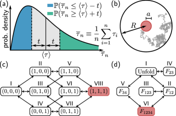
Figure 1: Deviations of empirical first-passage times from the true mean and model systems. (a) Schematic probability density of empirical first-passage time $\overline{\tau}_{n}$ inferred from a sample of $n$ realizations of an ergodic reversible Markov process. The tail probability that the estimate $\overline{\tau}_{n}$ deviates from the true mean $\langle\tau\rangle$ by more or equal than $t$ upwards $\mathbbm{P}(\overline{\tau}_{n}\geq\langle\tau\rangle+t)$ or downwards $\mathbbm{P}(\overline{\tau}_{n}\leq\langle\tau\rangle-t)$ is shown in green and blue, respectively. (b) Brownian molecular search process in a $d$-dimensional domain (here $d=2$) with outer radius $R$ and target radius $a$. Discrete-state Markov jump models of protein folding for (c) a toy protein and (d) experimentally inferred model of calmodulin [129]. Transitions between states obey detailed balance and absorbing targets are colored red.

Computer simulations often especially suffer from insufficient sampling, which leads to substantial errors in inferred rates [133, 134, 135, 136] and, in the worst case, erroneous conclusions (see discussion in [118, 137]). Even extensive computing resources may result in only a few independent estimates spread over many orders of magnitude, rendering uncertainty quantification challenging and not amenable to standard error analysis [121].
Constructing reliable confidence intervals is a fundamental challenge in statistical inference, and many prevalent methods only hold when $n\to\infty$. The applicability of such asymptotic results in a finite-sample setting is, by definition, problematic. In particular, Central-Limit- and bootstrapping-based methods may easily underestimate the uncertainty for small $n$ and fail to guarantee coverage of the confidence level [139, 140, 141, 142, 143, 144, 121].
Conversely, Bayesian methods (e.g. [145]), despite not relying on asymptotic arguments, must be treated with care, as estimates and their uncertainties are sensitive to, dependent on, and potentially biased by, the specification of the prior distribution, especially in the small-sample setting [120, 146] (see [128, 147, 134, 148, 149] for kinetic inference). Moreover, prior-dependent uncertainty estimates seem to remain, even in the asymptotic limit, an elusive problem (see extended discussion in [150]).
There is thus a pressing need for understanding fluctuations of inferred empirical first-passage times, a rigorous error control, and reliable non-asymptotic error estimation in the small-sample regime. These are fundamental unsolved problems of statistical kinetics and are essential for the analysis of experimental and simulation data.
Here, we present general bounds on fluctuations of empirical first-passage times that allow a rigorous uncertainty quantification (e.g. using confidence intervals with guaranteed coverage probabilities for all sample sizes) under minimal assumptions. We prove non-asymptotic lower ($\mathcal{L}$) and upper ($\mathcal{U}$) bounds on the deviation probability $\mathbbm{P}(\overline{\tau}_{n}\geq\langle\tau\rangle+t)$ and $\mathbbm{P}(\overline{\tau}_{n}\leq\langle\tau\rangle-t)$ (see Fig. 1a), i.e., the probability that the empirical first-passage time inferred from a sample of $n\geq 1$ realizations of an ergodic reversible Markov process, $\overline{\tau}_{n}$, deviates from the true mean $\langle\tau\rangle$ by more than $t$ in either direction,

$$\mathcal{L}^{\pm}_{n}(t)\leq\mathbbm{P}(\pm[\overline{\tau}_{n}-\langle\tau\rangle]\geq t)\leq\mathcal{U}_{n}^{\pm}(t)\quad\forall t\geq 0,$$ (1)

the upper bounds $\mathcal{U}_{n}^{\pm}(t)$ corresponding to so-called concentration inequalities [151]. The most conservative version of the derived upper bounds is independent of any details about the underlying dynamics. We use the bounds $\mathcal{U}^{\pm}_{n}(t)$ to quantify the uncertainty of the inferred sample mean $\overline{\tau}_{n}$ in a general setting and under minimal assumptions, for all $n\geq 1$. We further derive general lower ($\underline{\mathcal{M}}$) and upper ($\macc@depth\char 1\relax\frozen@everymath{\macc@group}\macc@set@skewchar\macc@nested@a 111{\mathcal{M}}$) bounds on the expected minimum $\tau_{n}^{-}=\min_{i\in[1,n]}\tau_{i}$ and maximum $\tau_{n}^{+}=\max_{i\in[1,n]}\tau_{i}$ of $n$ realizations, i.e.

$$\underline{\mathcal{M}}_{n}^{\pm}\leq\langle\tau^{\pm}_{n}-\langle\tau\rangle\rangle\leq\macc@depth\char 1\relax\frozen@everymath{\macc@group}\macc@set@skewchar\macc@nested@a 111{\mathcal{M}}_{n}^{\pm}\quad\forall n\geq 1,$$ (2)

controlling the uncertainty of first-passage times even when multiple time-scales are involved, rendering $\langle\tau\rangle$ an a priori insufficient statistic. The validity and sharpness of bounds are demonstrated by means of spatially confined Brownian search processes in dimensions 1 and 3 (Fig. 1b), and discrete-state Markov jump models of protein folding for a toy protein  [152, 134, 153, 45] (Fig. 1c) and the experimentally inferred model of calmodulin [129] (Fig. 1d). We conclude with a discussion of the practical implications of the results and further research directions.

Setup.—We consider time-homogeneous Markov processes $x_{t}$ on a continuous or discrete state-space $\Omega$ with generator $\hat{L}$ corresponding to a Markov rate-matrix or an effectively one-dimensional Fokker-Planck operator. Let the transition probability density to find $x_{t}$ at $x$ at time $t$ given that it evolved from $x_{0}$ be $p_{t}(x|x_{0})\equiv\mathrm{e}^{\hat{L}t}\delta_{x_{0}}(x)$ where $\delta_{x_{0}}(x)$ denotes the Dirac or Kronecker delta for continuous and discrete state-spaces, respectively. We assume the process to be ergodic $\lim_{t\to\infty}p_{t}(x|x_{0})=p_{\rm eq}(x)$, where $p_{\rm eq}(x)\equiv\mathrm{e}^{-\varphi(x)}$ denotes the equilibrium probability density and $\varphi(x)$ the generalized potential in units of thermal energy $k_{\rm B}T$ [154]. We assume that $\hat{L}$ obeys detailed balance and is either (i) bounded, (ii) $\Omega$ is finite with reflecting boundary $\partial\Omega$, or (iii) $\Omega$ is infinite but $\varphi(x)$ sufficiently confining (see ). Each of the conditions (i)-(iii) ensures that the spectrum of $\hat{L}$ is discrete .

We are interested in the first-passage time to a target $a$ when $x_{t=0}$ is drawn from a density $p_{0}(x)$

$$\tau=\inf_{t}[\,t\,|x_{t}=a,\,p_{0}(x_{0})],$$ (3)

and focus on the setting $p_{0}(x)=\tilde{p}_{\rm eq}(x)$, since $x_{0}$ usually cannot be controlled experimentally (see e.g., [39, 38, 65, 62, 61, 134, 158, 159]), and the tilde denotes that the absorbing state is excluded (see Appendix Ia for details). For completeness we also provide results for general initial conditions $p_{0}(x)$ in Appendix Ib and that require more precise conditions on $\varphi(x)$. The probability density of $\tau$ for such processes has the generic form [44, 45]

$$\wp_{a}(t|x_{0})=\sum_{k>0}\mu_{k}w_{k}^{x_{0}}{\rm e}^{-\mu_{k}t},$$ (4)

with first-passage rates $\mu_{k}>0$ and (not necessarily positive) spectral weights $w_{k}^{x_{0}}$ normalized according to $\sum_{k>0}w_{k}^{x_{0}}=1$ and $w_{1}^{x_{0}}>0$. The $m$-th moment of $\tau$ is given by $\langle\tau^{m}\rangle=m!\sum_{k>0}w^{x_{0}}_{k}/\mu_{k}^{m}$ and the survival probability reads $\mathbbm{P}(\tau>t)\equiv S_{a}(t|x_{0})=\sum_{k>0}w_{k}^{x_{0}}{\rm e}^{-\mu_{k}t}$. If $x_{0}$ is drawn from the equilibrium density, $\tilde{p}_{\rm eq}(x)$, we have $\wp_{a}(t|\tilde{p}_{\rm eq})\equiv\int_{\Omega\setminus a}\wp_{a}(t|x_{0})\tilde{p}_{\rm eq}(x_{0})dx_{0}$  which renders all weights non-negative, ${w_{k}\,\equiv\,\int_{\Omega\setminus a}w_{k}^{x_{0}}\tilde{p}_{\rm eq}dx_{0}\geq 0}$ (see proof in [150]). We henceforth abbreviate ${S_{a}(t|\tilde{p}_{\rm eq})\equiv S_{a}(t)}$.

To exemplify the need for uncertainty bounds in Eq. (1) we show in Fig. 2a-d that the probability that ${\overline{\tau}_{n}-\langle\tau\rangle}$ lies within a desired range of say $\pm$ 10% of the longest first-passage time scale $\mu_{1}^{-1}$, $\mathbbm{P}(\mu_{1}[\overline{\tau}_{n}-\langle\tau\rangle]\in[-0.1,0.1])$ is low even for $n\approx 50$ for all models in Fig. 1b-d. This inherent intrinsic noise-floor of the inferred observable $\overline{\tau}_{n}$ for any $n$ is embodied in, and can be explicitly demonstrated by, the existence of lower bounds $\mathcal{L}^{\pm}_{n}$ (see Appendix II).

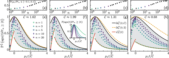
Figure 2: Deviation probabilities and corresponding bounds for a spatially confined Brownian search process in (a,e) $d=1$ and (b,f) $d=3$ dimensions, and Markov-jump models of protein folding for (c,g) the experimentally inferred model of calmodulin and (d,h) the toy protein. (a-d) Probability that $\delta\overline{\tau}_{n}=\overline{\tau}_{n}-\langle\tau\rangle$ lies within a range of $\pm 10\%$ of the longest time-scale $1/\mu_{1}$, $\mathbbm{P}(\mu_{1}\delta\overline{\tau}_{n}\in[-0.1,0.1])$, as a function of $n$ determined from the statistics of $\overline{\tau}_{n}$ for different fixed $n$ for all model systems. (e-h) Scaled probabilities $\mathbbm{P}^{1/n}(\text{sgn}(t)\delta\overline{\tau}_{n}\geq|t|)$ that the sample mean $\overline{\tau}_{n}$ inferred from $n$ realizations deviates from $\langle\tau\rangle$ by more than $t$ in either direction. Right tail areas are shown for $t>0$ and left for $t<0$, respectively. Lower $\mathcal{L}^{\pm}_{n}(t)$ and upper $\mathcal{U}^{\pm}_{n}(t;\mathcal{C})$ bounds are depicted as red and black lines, respectively, and the model-free upper bound $\mathcal{U}^{\pm}_{n}(t;2)$ as the dashed yellow line. Symbols denote corresponding scaled empirical deviation probabilities as a function of $t$ and are sampled for different $n$.

Cramér-Chernoff bounds.—To tackle this issue we now prove upper bounds using the Cramér-Chernoff approach. Let $\delta\overline{\tau}_{n}\equiv|\overline{\tau}_{n}-\langle\tau\rangle|$ and $\lambda\in\mathbbm{R}^{+}$. We start with the inequality $\mathrm{e}^{\lambda t}\mathbbm{1}_{\delta\overline{\tau}_{n}\geq t}\leq\mathrm{e}^{\lambda\delta\overline{\tau}_{n}}$, where $\mathbbm{1}_{b}$ is the indicator function of the set $b$. Taking the expectation yields $\mathbbm{P}(\delta\overline{\tau}_{n}\geq t)\leq\mathrm{e}^{-\lambda t}\langle\mathrm{e}^{\lambda\delta\overline{\tau}_{n}}\rangle\equiv\mathrm{e}^{-\lambda t+\psi_{\delta\overline{\tau}_{n}}(\lambda)}$, where we defined the cumulant generating function of $\delta\overline{\tau}_{n}$ as $\psi_{\delta\overline{\tau}_{n}}(\lambda)\equiv\ln\langle\mathrm{e}^{\lambda\delta\overline{\tau}_{n}}\rangle$. Note that $\tau_{i}$ are statistically independent. The bound can be optimized to find Chernoff’s inequality $\mathbbm{P}(\delta\overline{\tau}_{n}\geq t)\leq\mathrm{e}^{-n\psi^{*}_{\delta\tau}(t)}$ where $\psi^{\ast}_{\delta\tau}(t)$ is the Cramér transform of $\psi_{\delta\tau}(\lambda)$ [151],

$$\psi^{\ast}_{\delta\tau}(t)\equiv\sup_{\lambda}(\lambda t-\psi_{\delta\tau}(\lambda)),$$ (5)

with $\delta\tau\equiv\delta\overline{\tau}_{1}$. On the interval $\lambda\in[0,\mu_{1})$ we have the following bounds on $\psi_{\delta\tau}(\lambda)$ (see proof in [150])

$$\psi_{\delta\tau}(\lambda)\leq\phi_{\delta\tau}(\lambda;\mathcal{C})\equiv\begin{dcases}\frac{\lambda^{2}}{2\mu_{1}^{2}}\frac{\mathcal{C}}{1-\lambda/\mu_{1}}&\tau\geq\langle\tau\rangle\\ \frac{\lambda^{2}}{2\mu_{1}^{2}}\frac{\mathcal{C}}{1-(\lambda/\mu_{1})^{2}}&\tau<\langle\tau\rangle,\end{dcases}$$ (6)

which are non-negative, convex, and increasing on $\lambda\in[0,\mu_{1})$, and we introduced $\mathcal{C}\equiv\mu_{1}^{2}\langle\tau^{2}\rangle$. Note that general initial conditions $p_{0}(x_{0})$ are accounted for by simply replacing $\langle\tau^{2}\rangle$ in $\mathcal{C}$ (see Appendix Ib and [150] for details). The bound (6) further implies $\psi_{\delta\tau}^{*}(t)\geq\phi_{\delta\tau}^{*}(t;\mathcal{C})$, $\forall t\geq 0$, and may thus be optimized [161] to obtain the inequalities announced in Eq. (1) via Chernoff’s inequality:

$$\mathcal{U}_{n}^{+}(t;\mathcal{C}) =\exp\left(-n\mathcal{C}h_{+}\left(\mu_{1}t/\mathcal{C}\right)\right)\quad 0\leq t\leq\infty$$

$$\mathcal{U}_{n}^{-}(t;\mathcal{C}) =\exp\left(-n\mathcal{C}h_{-}\left(\mu_{1}t/\mathcal{C}\right)\right)\quad 0\leq t\leq\langle\tau\rangle$$ (7)

where we defined the functions

$$h_{+}(u) \equiv 1+u-\sqrt{1+2u}$$ (8)

$$h_{-}(u) \equiv\Lambda(u)u-\frac{1}{2}\frac{\Lambda(u)^{2}}{1-\Lambda(u)^{2}}$$ (9)

with $\Lambda(u)\equiv\frac{1}{2}\left[g(u)-\sqrt{4+2/g(u)u-g(u)^{2}}\right]$ and

$$\!g(u)\equiv\frac{2}{\sqrt{3}}\left\{1+2\cosh\left[\frac{1}{3}{\rm arcosh}\left(1+\frac{3^{3}}{2^{7}u^{2}}\right)\right]\right\}^{1/2}\!\!\!\!\!.$$ (10)

These results control the deviations of the inferred $\overline{\tau}_{n}$ from $\langle\tau\rangle$ for all $n$. Note that in general whenever $\mu_{1}\langle\tau\rangle\not\approx 1$ (e.g. in “compact” search processes [38, 39]), $\langle\tau\rangle$ is not necessarily representative due to the multiple relevant time-scales [63, 64, 65]. However, as we show below, $\langle\tau\rangle$ sharply bounds extreme first-passage times. Thus, inferring $\overline{\tau}_{n}$ provides insight about first-passage statistics even when $\langle\tau\rangle$ is a priori not a sufficient statistic.

Concerning practical applications, deviations are readily expressed relative to the longest natural time-scale $1/\mu_{1}$ that does not need to be known. That is, errors in units of $1/\mu_{1}$, $\mu_{1}(\overline{\tau}_{n}-\langle\tau\rangle)$, are naturally parameterized by the dimensionless variable $\mu_{1}t$. Remarkably, details about the underlying dynamics then only enter the bounds (7) via a system-dependent constant $\mathcal{C}$ that, however, can be bounded. In particular, for equilibrium initial conditions we have $0\leq 2w_{1}\leq\mathcal{C}\leq 2$ (see [150]). Since $\phi_{\delta\tau}$ is monotonically increasing with $\mathcal{C}\in(0,2]$, we have $\phi_{\delta\tau}(\lambda;\mathcal{C})\leq\phi_{\delta\tau}(\lambda;2)$ which implies $\phi^{*}_{\delta\tau}(t;\mathcal{C})\geq\phi^{*}_{\delta\tau}(t;2)$. Thus, we find the model-free bounds by setting $\mathcal{C}\equiv 2$

$$\mathcal{U}_{n}^{\pm}(t;\mathcal{C})\leq\mathcal{U}_{n}^{\pm}(t;2)\equiv\mathcal{U}_{n}^{\pm}(t)$$ (11)

requiring no information about the system. The non-asymptotic bounds on deviation probabilities of $\overline{\tau}_{n}$ in Eqs. (7) and (11) are our first main result. Their most general and conservative version states that for all sample-sizes $n$, the probability of observing a relative error larger than a specified value $\mu_{1}t$ (e.g., $\mu_{1}t=0.1$ or $10\%$), $\mathbbm{P}(\mu_{1}[\overline{\tau}_{n}-\langle\tau\rangle]\geq\mu_{1}t)$, is lower than the corresponding upper bound $\mathcal{U}_{n}^{\pm}(\mu_{1}t)$, which solely depends on $\mu_{1}t$.

Lastly, as $n\to\infty$, $\mathcal{U}^{\pm}_{n}$ is substantial only for $\mu_{1}t/\mathcal{C}\ll 1$ and the tails become symmetric and sub-Gaussian [151], $h_{+}(u)=u^{2}/2-\mathcal{O}(u^{3})$ and $h_{-}(u)=u^{2}/2-\mathcal{O}(u^{4})$ (see [150]). Notably, concentration inequalities were recently derived for time-averages of “classical” [162, 163, 164] (see ), and quantum [166] Markov processes, as well as inverse thermodynamic uncertainty relations [167].

Illustration of deviation bounds.—The upper $\mathcal{U}^{\pm}_{n}(t)$ and lower $\mathcal{L}^{\pm}_{n}(t)$ bounds on $\mathbbm{P}(\pm[\overline{\tau}_{n}-\langle\tau\rangle]\geq t)$ in Eqs. (7) and (15), respectively, are examplified in Fig. 2e-h (see black and red lines) for the model systems shown in Fig. 1b-d. Note that to illustrate all bounds we formally let $t\to-t$ for the left tails $\mathcal{L}^{-}_{n}(t)$ and $\mathcal{U}^{-}_{n}(t)$, such that their support is on $[-\langle\tau\rangle,\infty)$. Deviation probabilities are in turn expressed as $\mathbbm{P}(\text{sgn}(t)\delta\overline{\tau}_{n}\geq|t|)$ where $\text{sgn}(x)$ denotes the signum function and $\delta\overline{\tau}_{n}=\overline{\tau}_{n}-\langle\tau\rangle$.

To assess the quality of our bounds we scale probabilities $\mathbbm{P}^{1/n}$ such that $\mathcal{L}^{\pm}_{n}(t)$ and $\mathcal{U}^{\pm}_{n}(t)$ collapse onto a master curve for all $n$ (see inset Fig. 2f). Symbols denote empirical deviation probabilities obtained by sampling $\overline{\tau}_{n}$ for different $n$ (see [150] for details), which approach the upper bound as $n$ increases. For $n=1$ right-tail deviations are close to $\mathcal{L}^{+}_{1}(t)$ even for $w_{1}\leq 1$ . As expected the model-free bound $\mathcal{U}^{\pm}_{n}(t;2)$ (yellow) holds universally but is generally more conservative. Notably, it remains remarkably good even for $\mathcal{C}\gtrsim 1.3$ (Fig. 2e-g).
Uncertainty quantification.—The bounds (7) and (11) provide the elusive systematic framework to rigorously quantify the uncertainty of the estimate $\overline{\tau}_{n}$ for any, and especially for small, sample sizes. In particular, they allow the construction of “with high probability” guarantees such as confidence intervals, which—unlike traditional confidence intervals in statistics—are not only asymptotically correct but hold for any $n$. Concentration-based guarantees do further not require specifying a prior belief as in the Bayesian context. Setting $\mathcal{U}_{n}^{\pm}(t^{\pm}_{\alpha_{\pm}};\mathcal{C})=\alpha_{\pm}$ for chosen acceptable left- and right-tail error probabilities $\alpha_{\pm}$ (with $\alpha_{+}+\alpha_{-}<1$), we get an implicit definition of the confidence interval $[-t^{-}_{\alpha_{-}},t^{+}_{\alpha_{+}}]$ at confidence level (or “coverage probability”) $1-(\alpha_{-}+\alpha_{+})$ in the form

$$\mathbbm{P}(-t^{-}_{\alpha_{-}}\leq\delta\overline{\tau}_{n}\leq t^{+}_{\alpha_{+}})\geq 1-\alpha_{-}-\alpha_{+}\equiv 1-\alpha,$$ (12)

stating that with probability of at least $1-\alpha$ the sample mean $\overline{\tau}_{n}$ lies within $[\langle\tau\rangle-t^{-}_{\alpha_{-}},\langle\tau\rangle+t^{+}_{\alpha_{+}}]$. Confidence intervals are closely related to, and can be used for, statistical significance tests [169, 170], and beyond that provide quantitative bounds on statistical uncertainty. Two-sided central confidence intervals for $\delta\overline{\tau}_{n}$ as a function of $n$ for a confidence level of $\alpha=0.1$ and models systems in Fig. 1b-d are shown (rescaled to a master scaling) in Fig. 3a (for a detailed discussion see [150]).

In particular, we may now also answer the practical question: How many realizations are required to achieve a desired accuracy with a specified probability? To ensure with probability of at least $1-\alpha$ that $\delta\overline{\tau}_{n^{*}}\in[-t^{-}_{\alpha_{-}},t^{+}_{\alpha_{+}}]$ one needs a minimal sample size $n^{*}$ defined via

$$\mathcal{U}_{n^{\ast}}^{+}(t^{+}_{\alpha_{+}};\mathcal{C})+\mathcal{U}_{n^{\ast}}^{-}(t^{-}_{\alpha_{-}};\mathcal{C})=\alpha.$$ (13)

The number of samples $n^{\ast}$ required to guarantee that $\overline{\tau}_{n^{*}}$ falls within a symmetric interval of length $\Delta t=0.2/\mu_{1}$, (i.e. $\overline{\tau}_{n^{*}}\in[\langle\tau\rangle-0.1/\mu_{1},\langle\tau\rangle+0.1/\mu_{1}]$) with probability of at least $1-\alpha$ is shown in Fig. 3b for several values of $\mathcal{C}$ (intersections with the dashed line yield $n^{\ast}$ guaranteeing a coverage of at least 90%). Fig. 3c depicts the complementary symmetric interval $\Delta t$ covering the range of $\delta\overline{\tau}_{n}$ for a given $n$ with probability of at least 90%. Note that hundreds to thousands of samples may be required to ensure an accuracy of $\pm 0.1/\mu_{1}$ with a 90% confidence, which is seemingly not met in experiments [119, 120, 118, 121, 122, 123, 124].
Eqs. (12-13) can be solved for $t^{\pm}_{\alpha_{\pm}}$ and $n^{\ast}$, respectively, using standard root-finding methods (see [150]) and constitute our second main result. They allow for rigorous error control in kinetic inference in the small-$n$ regime.

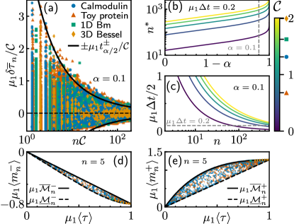
Figure 3: Non-asymptotic uncertainty quantification of the sample mean $\overline{\tau}_{n}$ and extreme deviations from $\langle\tau\rangle$. (a) Relative error $\mu_{1}\delta\overline{\tau}_{n}=\mu_{1}(\overline{\tau}_{n}-\langle\tau\rangle)$ (symbols) obtained from sampling of $\overline{\tau}_{n}$ for different $n$ and model systems. The central confidence interval $[-\mu_{1}t^{-}_{\alpha/2},\mu_{1}t^{+}_{\alpha/2}]$ with $\alpha=0.1$ in black. (b) Number of samples $n^{*}$ to ensure that the error $\mu_{1}\delta\overline{\tau}_{n^{*}}$ falls in the interval $[-0.1,0.1]$ of length $\Delta t=0.2/\mu_{1}$ with probability of at least $1-\alpha$ for several values of $\mathcal{C}$. (c) Symmetric confidence interval $[-\mu_{1}\Delta t/2,\mu_{1}\Delta t/2]$ (upper limit shown) for $\alpha=0.1$ as a function of $n$ for different $\mathcal{C}$. Average extreme deviation from the mean $\langle m_{n}^{\pm}\rangle\equiv\langle\tau^{\pm}_{n}-\langle\tau\rangle\rangle$ (symbols) and bounds (lines) for the minimum (d) and maximum (e) of $n=5$ realizations for different models and values of $\mu_{1}\langle\tau\rangle$.

Using Eq. (11) we can further construct system-independent but more conservative universal confidence intervals (see yellow line in Fig. 3b,c). Interestingly, even when $\mathcal{C}\approx 1$ the universal bound remains reasonably tight, only for $\mathcal{C}\ll 1$ differences become substantial.
Bounding extreme deviations.—Finally, we show that $\langle\tau\rangle$ controls the range of inferred $\tau_{i}$ in any sample of $n$ independent realizations, i.e., it sharply bounds the average minimum $\tau_{n}^{-}$ and maximum $\tau_{n}^{+}$ deviations from the mean $m^{\pm}_{n}\equiv\tau^{\pm}_{n}-\langle\tau\rangle$. As our third main results we prove (see sketch of proof and saturation conditions in Appendix III and [150] for details) two-sided bounds $\underline{\mathcal{M}}_{n}^{\pm}\leq\langle m^{\pm}_{n}\rangle\leq\macc@depth\char 1\relax\frozen@everymath{\macc@group}\macc@set@skewchar\macc@nested@a 111{\mathcal{M}}_{n}^{\pm}$, where

$$\!\!\underline{\mathcal{M}}_{n}^{+}\equiv\langle\tau\rangle\sum_{k=2}^{n}\frac{1}{k},\,\,\,\,\macc@depth\char 1\relax\frozen@everymath{\macc@group}\macc@set@skewchar\macc@nested@a 111{\mathcal{M}}_{n}^{+}\!\equiv\!\sum_{k=1}^{n}\!\binom{n}{k}(-1)^{k+1}\frac{(\mu_{1}\langle\tau\rangle)^{k}}{\mu_{1}k}-\langle\tau\rangle$$ (14)

$$\!\!\underline{\mathcal{M}}_{n}^{-}\equiv\langle\tau\rangle\!\left[n^{-1}(\mu_{1}\langle\tau\rangle)^{n-1}-1\right],\,\,\,\,\,\,\macc@depth\char 1\relax\frozen@everymath{\macc@group}\macc@set@skewchar\macc@nested@a 111{\mathcal{M}}^{-}_{n}\equiv\langle\tau\rangle\!\left[n^{-1}-1\right].$$

Remarkably, the tight bounds on $\mu_{1}\langle m^{\pm}_{n}\rangle$ are completely specified by the dimensionless parameter $\mu_{1}\langle\tau\rangle$. This motivates the inference of $\overline{\tau}_{n}$ in a general setting, even when $\langle\tau\rangle$ is a priori not representative, since via the bounds (14) (shown in Fig. 3d-e) $\langle\tau\rangle$ controls the range of estimates. The bounds (14) provide insight about the slowest and fastest out of $n$ first-passage times, and are thus relevant in the “few encounter” limit [44, 46, 47, 171].
Conclusion.—Leveraging spectral analysis and the framework of concentration inequalities we derived general upper and lower bounds on the probability that the empirical first-passage time $\overline{\tau}_{n}$ inferred from $n$ independent realizations deviates from the true mean $\langle\tau\rangle$ by any given amount. Using these bounds we constructed non-asymptotic confidence intervals that hold in the elusive small-sample regime and thus go beyond Central-Limit- and bootstrapping-based methods which fail for small $n$. The results require minimal input and in particular do not require any prior belief as in the Bayesian approach that is known to be problematic and likely underestimates the uncertainty in sub-sampling settings. Our concentration-based results and bounds on extreme deviations allow for rigorous, model-free error control and reliable error estimation, which is essential for the analysis of experimental and simulation data. They may further be extended to non-ergodic and irreversible dynamics.

Acknowledgments.—Financial support from Studienstiftung des Deutschen Volkes (to R.B.) and the German Research Foundation (DFG) through the Emmy Noether Program GO 2762/1-2 (to A.G.) is gratefully acknowledged.

Appendix Ia: Equilibrium initial conditions.—We mainly consider that the initial value $x_{0}$ of the first-passage process is drawn from a “quasi” stationary equilibrium density $\tilde{p}_{\rm eq}(x)$. However, compared to standard relaxation processes with “true” stationary density $p_{\rm eq}(x)$, an appropriate definition of $\tilde{p}_{\rm eq}(x)$ for absorption (i.e., first-passage) processes is more subtle as the absorbing target $a$ has to be accounted for. In discrete state-space we have $\tilde{p}_{\rm eq}(x_{k\neq a})\equiv p_{\rm eq}(x_{k})/\sum_{k\neq a}p_{\rm eq}(x_{k})$, i.e., the quasi-stationary density $\tilde{p}_{\rm eq}(x)$ is obtained via renormalization of $p_{\rm eq}(x)$ by excluding the target $a$. On the contrary, in the continuous state-space setting, the absorbing state $a$ has nominally zero measure such that trivially $\tilde{p}_{\rm eq}(x)=p_{\rm eq}(x)$ remains unchanged.

Appendix Ib: Arbitrary initial conditions.— Unless the state space $\Omega$ is both discrete and finite, an extension to arbitrary initial conditions, where $x_{0}$ is drawn from a general density $p_{0}(x)$, requires some additional assumptions about the generalized potential $\varphi(x)$. In particular, when $p_{0}(x)\neq\tilde{p}_{\rm eq}(x)$, $\varphi(x)$ must be sufficiently confining to ensure a “nice” asymptotic growth of eigenvalues $\nu_{k}$ of $\hat{L}$ of the relaxation dynamics [157], i.e., $\lim_{k\to\infty}\nu_{k}=bk^{\beta}$ with $\beta>1/2$ and $0<b<\infty$. The latter condition is automatically satisfied when $\Omega$ is finite, since regular Sturm-Liouville problems display Weyl asymptotics with $\beta=2$ [172]. The condition is in fact satisfied by most physically relevant processes with discrete spectra, including the (Sturm-Liouville irregular) Ornstein-Uhlenbeck or Rayleigh process [173] with $\beta=1$.

Manifestations of general initial conditions $p_{0}(x_{0})\neq\tilde{p}_{\rm eq}(x_{0})$ are then fully accounted for by simply replacing $\langle\tau^{2}\rangle$ with $2\sum_{i}w_{i}\mathbbm{1}_{w_{i}>0}/\mu_{i}^{2}<\infty$ in the presented results, i.e., $\mathcal{C}\to 2\sum_{i}w_{i}\mathbbm{1}_{w_{i}>0}(\mu_{1}/\mu_{i})^{2}$. Additional details, such as a proof of convergence of the sum $\sum_{i}w_{i}\mathbbm{1}_{w_{i}>0}/\mu_{i}^{2}$, are given in [150].

Appendix II: Lower bounds on deviation probabilities.— There exists a “noise floor” in the estimate $\overline{\tau}_{n}$ for any $n$. Since $\mu_{k}\leq\mu_{k+1}$ and the weights are non-negative $w_{k}\geq 0$ [150] and normalized [44, 45], the survival probability obeys the bound $w_{1}{\rm e}^{-\mu_{1}t}\leq S_{a}(t)\leq{\rm e}^{-\mu_{1}t}$. Using that $\overline{\tau}_{n}\geq\tau_{n}^{\rm-}$ and $\overline{\tau}_{n}\leq\tau_{n}^{\rm+}$ it follows immediately that $\mathbbm{P}(\tau_{n}^{-}\geq t)\leq\mathbbm{P}(\overline{\tau}_{n}\geq t)\leq\mathbbm{P}(\tau_{n}^{+}\geq t)$. Furthermore, we have $\mathbbm{P}(\tau_{n}^{-}\geq t)=S_{a}(t)^{n}$ as well as $\mathbbm{P}(\tau_{n}^{+}\leq t)=(1-S_{a}(t))^{n}$ such that we arrive at the lower bounds

$$\mathbbm{P}\left({\overline{\tau}_{n}-\langle\tau\rangle\geq t}\right) \geq\left(w_{1}{\rm e}^{-\mu_{1}(\langle\tau\rangle+t)}\right)^{n}\equiv\mathcal{L}_{n}^{+}(t)$$

$$\mathbbm{P}\left({\overline{\tau}_{n}-\langle\tau\rangle\leq-t}\right) \geq\left(1-{\rm e}^{-\mu_{1}(\langle\tau\rangle-t)}\right)^{n}\equiv\mathcal{L}_{n}^{-}(t).$$ (15)

We remark that analogous results are also obtained for upper bounds (see [150]) which, however, are weaker than those derived above in Eqs. (7) and (11) with the Cramér-Chernoff approach and concurrently require more information about the dynamics.

Appendix III: Sketch of proof of extreme-deviation bounds and their saturation.—In essence, the proofs of “squeeze” bounds $\underline{\mathcal{M}}_{n}^{\pm}\leq\langle m^{\pm}_{n}\rangle\leq\macc@depth\char 1\relax\frozen@everymath{\macc@group}\macc@set@skewchar\macc@nested@a 111{\mathcal{M}}_{n}^{\pm}$ rely on bounding the average value of the minimum $\tau^{-}_{n}\equiv\min_{i\in[1,n]}\tau_{i}$ or maximum $\tau^{+}_{n}\equiv\max_{i\in[1,n]}\tau_{i}$ out of $n$ first-passage times. As a first step recall that $\tau_{i}$’s are i.i.d., such that we may write $\langle\tau_{n}^{\pm}\rangle=\int_{0}^{\infty}\mathbbm{P}(\tau^{\pm}_{n}>t)dt$ solely in terms of the survival probability $S_{a}(t)$, that is,

$$\langle\tau^{+}_{n}\rangle =\int_{0}^{\infty}[1-(1-S_{a}(t))^{n}]dt$$

$$\langle\tau^{-}_{n}\rangle =\int_{0}^{\infty}S_{a}(t)^{n}dt.$$ (16)

This enables us to fully exploit the mathematical structure of the spectral decomposition of $S_{a}(t)$, allowing us to ultimately arrive at Eq. (14) by bounding the respective integrands in Eq. (16).

To briefly outline the key ideas, bounds $\underline{\mathcal{M}}_{n}^{-}$ and $\macc@depth\char 1\relax\frozen@everymath{\macc@group}\macc@set@skewchar\macc@nested@a 111{\mathcal{M}}_{n}^{+}$ follow by recognizing (since $\wp_{a}(t|\tilde{p}_{\rm eq})$ is monotonic in $t$) that $\langle\tau^{+}_{n}\rangle$ is maximal and $\langle\tau^{-}_{n}\rangle$ is minimal, respectively, whenever the contribution $w_{1}/\mu_{1}$ of the longest first-passage time-scale is maximal. For any fixed value of $\mu_{1}\langle\tau\rangle\in(0,1]$, this condition is generally met in the presence of a spectral gap $\mu_{1}/\mu_{k}\to 0,\forall k>1$, for which one may utilize in Eq. (16) the ansatz

$$S_{a}(t)=\lim_{\varepsilon\to 0}(1-\mu_{1}\langle\tau\rangle){\rm e}^{-t/\varepsilon}+\mu_{1}\langle\tau\rangle{\rm e}^{-\mu_{1}t}.$$ (17)

The announced bounds are consequently obtained after some straightforward calculations and become saturated (i.e. the inequality becomes an equality) in systems with the above stated spectral gap [150].
The main idea behind proving the bound $\underline{\mathcal{M}}_{n}^{+}$ relies on the inequality $S_{a}(t)\geq w_{k_{+}}{\rm e}^{-\mu_{k_{+}}t}$, were $k_{+}\equiv{\rm argmin}_{k}w_{k}>0$ denotes the smallest $k$ for which the corresponding weight $w_{k}$ is strictly positive. Saturation occurs when $w_{k_{+}}\to 1$.
The remaining bound $\macc@depth\char 1\relax\frozen@everymath{\macc@group}\macc@set@skewchar\macc@nested@a 111{\mathcal{M}}_{n}^{-}$ follows directly from upper bounding the convex function $x^{n}$, $\forall n\geq 1$, $x\geq 0$, by means of Jensen’s inequality and is saturated when $w_{k}\to 1$ for some $k$ and for degenerate systems with identical first-passage eigenvalues $\mu_{i}=\mu,\forall i$ for some $\mu>0$.

In this Supplementary Material (SM) we present a discussion of issues arising when applying Bayesian inference in the small-sample regime, additional background and details of the calculations, auxiliary results, numerical methods, and mathematical proofs of the claims made in the Letter. The sections are organized in the order as they appear in the Letter.

S1 Issues with Bayesian inference in the small-sample regime

Here we continue and extend the discussion on issues arising in Bayesian inference in the small-sample regime and conclude with difficulties that may even arise in the asymptotic large-sample limit. Bayesian methods (see e.g. [1]) do not rely on asymptotic arguments and are therefore often (in general erroneously [2, 3]) believed to readily alleviate the small-sample problem. Bayesian estimates are highly sensitive to, dependent on, and potentially biased by, the specification of the prior distribution, especially in the small-sample setting [1, 4, 5, 6]. Due to the prior dependence of estimates and their uncertainties, Bayesian methods must be treated with care when applied to small samples [7, 8] (see [9, 10, 11, 12, 13] specifically for kinetic inference) and can perform worse than asymptotic frequentist methods [7].

Moreover, so-called “credible intervals”—the Bayesian analogue to confidence intervals—have a nominally different meaning, as they treat the estimated parameter as a random variable. Bayesian posterior intervals are similarly affected by limited sampling [14], i.e. the constructed uncertainty estimates and their quality are sensitive to the choice of prior probability [2, 3] and may likely underestimate the true uncertainty and thus fail to provide trustworthy confidence intervals [15, 11].

On a more subtle level, the classical Bernstein-von-Mises theorem establishes a rigorous (frequentist) justification of posterior-based Bayesian credible intervals as asymptotically correct, prior independent confidence intervals for (finite dimensional) parametric models in the large-sample limit [16, 17, 18]. Analogous statements for semi-parametric and (infinite dimensional) non-parametric models, however, involve more delicate conceptual and mathematical issues [19, 20, 21, 22] and, despite having received significant attention [23, 24, 25, 26, 27, 28, 29, 30, 31, 32, 33, 34] (see also [35] for misspecified and high dimensional [36] parametric models), seem to remain—even in the asymptotic, large-sample regime—an elusive problem.

S2 Spectral representation and preparatory Lemmas

In this section we provide additional background on the spectral analysis of first-passage problems and some auxiliary Lemmas. In particular, we prove that for equilibrium initial conditions all spectral first-passage weights $w_{k}(\tilde{p}_{\rm eq})$ are non-negative and that for general initial conditions $p_{0}(x_{0})$ the sum of positive spectral weights is always bounded.

S2.1 Spectral representation and general results

First, we recall some general results using the spectral representation of first-passage processes (for more details see e.g. [37, 38]). As stated in the Letter, we consider time-homogeneous Markov processes $x_{t}$ on a continuous or discrete state-space $\Omega$ with (forward) generator $\hat{L}$ corresponding to a Markov rate-matrix or an effectively one-dimensional Fokker-Planck operator. Let the transition probability density to find $x_{t}$ at $x$ at time $t$ given that it evolved from $x_{0}$ be $p_{t}(x|x_{0})\equiv\mathrm{e}^{\hat{L}t}\delta_{x_{0}}(x)$ where $\delta_{x_{0}}(x)$ denotes the Dirac or Kronecker delta for continuous and discrete state-spaces, respectively. We assume the process to be ergodic $\lim_{t\to\infty}p_{t}(x|x_{0})=p_{\rm eq}(x)$, where $p_{\rm eq}(x)\equiv\mathrm{e}^{-\varphi(x)}$ denotes the equilibrium probability density and $\varphi(x)$ the corresponding generalized potential in units of thermal energy $k_{\rm B}T$. We assume that $\hat{L}$ obeys detailed balance, such that it is self-adjoint in the left eigenspace with respect to a scalar product weighted by $\mathrm{e}^{-\varphi(x)}$ and the operator $\mathrm{e}^{\varphi(x)/2}\hat{L}\mathrm{e}^{-\varphi(x)/2}$ is self-adjoint with respect to a flat measure.

We assume that $\hat{L}$ is either (i) bounded, (ii) $\Omega$ is finite with reflecting boundary $\partial\Omega$, or that (iii) $\Omega$ is infinite but $\varphi(x)$ is sufficiently confining (precisely, we require that $\varphi(x)$ satisfies the Poincaré inequality, i.e. $\lim_{|x|\to\infty}(|\nabla\varphi(x)|^{2}/2-\nabla^{2}\varphi(x))=\infty$). Each of the conditions (i)-(iii) ensures that the eigenvalue spectrum of $\hat{L}$ is discrete. The relaxation eigenvalue problem (for the inner product $(\cdot|\cdot)$ defined with respect to a flat Lebesgue measure) reads $-\hat{L}\Psi^{\rm R}_{k}(x)=\nu_{k}\Psi^{\rm R}_{k}(x)$ with $\Psi_{k}^{\rm L}(x)=\Psi^{\rm R}_{k}(x)\mathrm{e}^{\varphi(x)}$, $\nu_{0}=0$ and $\nu_{k\geq 1}>0$.

The first-passage time to a target $a$ for $x_{t=0}$ drawn from a density $p_{0}(x_{0})$ is defined as $\tau=\inf_{t}[\,t\,|x_{t}=a,\,p_{0}(x_{0})]$. We will use $\langle\cdot\rangle$ to denote an average over all first-passage paths $\{x_{t^{\prime}}\}_{0\leq t^{\prime}\leq\tau}$, i.e. those that hit $a$ only once. The first-passage time density to $a$, $\wp_{a}(t|x_{0})=\langle\delta(t-\tau[\{x_{t^{\prime}}\}])\rangle$ to reach the absorbing target at $x=a$, starting initially from $x_{0}$, has the general spectral representation

$$\wp_{a}(t|x_{0})=\sum_{k\geq 1}w_{k}{(x_{0})}\mu_{k}{\rm e}^{-\mu_{k}t},$$ (S1)

where $\mu_{k}$ is the $k$-th first-passage rate and $w_{k}(x_{0})$ its corresponding first-passage weight [37, 38]. In similar fashion the survival probability is expressed as

$$S_{a}(t|x_{0})\equiv\int_{t}^{\infty}\wp_{a}(t^{\prime}|x_{0})dt^{\prime}=\sum_{k\geq 1}w_{k}(x_{0}){\rm e}^{-\mu_{k}t}.$$ (S2)

We note that in contrast to the relaxation eigenvalues $\nu_{k}$, the first-passage rates $\mu_{k}=\mu_{k}(a)$ depend in the location of the absorbing target. Moreover, for any target location $a$ the interlacing theorem holds [37, 38] :

$$\nu_{k-1}\leq\mu_{k}(a)\leq\nu_{k}\quad\forall k,a$$ (S3)

where equality occurs iff $w_{k}(x_{0})=0$, i.e. for $a$ where $\Psi_{k}^{\rm R}(a)=0$.

Laplace transforming the spectral expansion of the first-passage time density (S1)—according to $\tilde{f}(s)\equiv\int{\rm e}^{-st}f(t)\,dt$ with $f$ being a generic function locally integrable on $t\in[0,\infty)$—yields

$$\tilde{\wp}_{a}(s)=\sum_{k\geq 1}\frac{w_{k}(x_{0})\mu_{k}}{s+\mu_{k}}.$$ (S4)

The first-passage weights are then obtained by using the residue theorem to invert the Laplace transformed renewal theorem [39, 37, 38]

$$w_{k}(x_{0})=\frac{\tilde{p}(a,-\mu_{k}|x_{0})}{\mu_{k}\dot{\tilde{p}}(a,-\mu_{k}|a)}=\frac{\sum_{l\geq 0}(1-\nu_{l}/\mu_{k})^{-1}\Psi_{l}^{\rm R}(a)\Psi_{l}^{\rm L}(x_{0})}{\sum_{l\geq 0}(1-\nu_{l}/\mu_{k})^{-2}\Psi_{l}^{\rm R}(a)\Psi_{l}^{\rm L}(a)}<\infty,$$ (S5)

where $\dot{\tilde{p}}(a,s|a)=\partial_{s}\tilde{p}(a,s|a)$ is taken at $s=-\mu_{k}$ and $\{\nu_{l},\Psi_{l}^{\rm R},\Psi_{l}^{\rm L}\}$ are the corresponding relaxation eigenmodes [37, 38]. The weights satisfy $\sum_{k\geq 1}w_{k}(x_{0})=1$ and the first non-zero weight is strictly positive $w_{1}(x_{0})>0$. Moreover, the relaxation eigenvalues $\nu_{0}=0$ and all $\nu_{k>0}\geq 0$ are real as a result of detailed balance.

S2.2 Lemma 1: All weights are non-negative for equilibrium initial conditions

In the Letter we focus on equilibrium initial conditions, that is we assume that $x_{0}$ is drawn from the invariant measure, $p_{\rm eq}(x_{0})$, which in the particular case of diffusion processes is assumed to have a reflecting boundary at $a$ (i.e. we focus on the one-sided first-passage process). We further introduce the non-negative modified spectral weights $\bar{w}_{k}(x_{0})\equiv w_{k}(x_{0})\theta(\operatorname{sgn}[w_{k}(x_{0})])$ and now prove that for a normalized equilibrium probability density of initial conditions $p_{0}(x_{0})$ that excludes the target—i.e. $\tilde{p}_{\rm eq}(x_{0})\equiv p_{\rm eq}(x_{0})[1-\delta_{a}(x_{0})]/(1|p_{\rm eq}(x_{0})[1-\delta_{a}(x_{0})])$ where $\delta_{a}(x_{0})$ is the Dirac measure (note that $(1|\tilde{p}_{\rm eq})=1$)—all weights $w_{k}$ are rendered non-negative. We thus have $\bar{w}_{k}(\tilde{p}_{\rm eq})=w_{k}(\tilde{p}_{\rm eq})\geq 0,\forall k$.

Namely, because $\Psi_{l}^{\rm L}(a)={\rm e}^{\varphi(a)}\Psi_{l}^{\rm R}(a)$ we have $\Psi_{l}^{\rm R}(a)\Psi_{l}^{\rm L}(a)\geq 0,\forall l$, and from bi-orthogonality $(\Psi_{l}^{\rm L}|p_{\rm eq})=\delta_{l,0}$ it follows that [with $\tilde{p}_{\rm eq}(a)=p_{\rm eq}(a)/(1-p_{\rm eq}(a))$]

$$\tilde{w}_{k}\equiv(w_{k}|\tilde{p}_{\rm eq})=\tilde{p}_{\rm eq}(a)\frac{1-\sum_{l\geq 0}(1-\nu_{l}/\mu_{k})^{-1}\Psi_{l}^{\rm R}(a)\Psi_{l}^{\rm L}(a)}{\sum_{l\geq 0}(1-\nu_{l}/\mu_{k})^{-2}\Psi_{l}^{\rm R}(a)\Psi_{l}^{\rm L}(a)}=\frac{\tilde{p}_{\rm eq}(a)}{\sum_{l\geq 0}(1-\nu_{l}/\mu_{k})^{-2}\Psi_{l}^{\rm R}(a)\Psi_{l}^{\rm L}(a)}\geq 0,$$ (S6)

because by definition $\mu_{k}>0,\forall k\geq 1$ denotes the zeros of $\tilde{p}(a,s|a)$, i.e. $\tilde{p}(a,-\mu_{k}|a)=\sum_{l\geq 0}(\nu_{l}-\mu_{k})^{-1}\Psi_{l}^{\rm R}(a)\Psi_{l}^{\rm L}(a)=\mu_{k}^{-1}\sum_{l\geq 0}(1-\nu_{l}/\mu_{k})^{-1}\Psi_{l}^{\rm R}(a)\Psi_{l}^{\rm L}(a)=0$ which completes the proof of the Lemma.

S2.3 Lemma 2: Sum of positive weights is bounded from above

For the sake of completeness we present supplementary results for general initial conditions $p_{0}(x_{0})$. Recall from the Letter that we require some additional conditions on $\varphi(x)$ or $\Omega$ in this more general setting.

In particular, we assume that $\varphi(x)$ is sufficiently confining to assure a “nice” asymptotic growth of eigenvalues, $\lim_{k\to\infty}\nu_{k}=bk^{\beta}$ with $\beta>1/2$ and $0<b<\infty$. The latter condition is automatically satisfied when $\Omega$ is finite, since regular Sturm-Liouville problems display Weyl asymptotics with $\beta=2$ [40]. The condition is in fact satisfied by most physically relevant processes with discrete spectra, including the (Sturm-Liouville irregular) Ornstein-Uhlenbeck or Rayleigh process [41] with $\beta=1$. This implies, by the interlacing theorem (S3) that $b(k-1)^{\beta}\leq\mu_{k}\leq bk^{\beta}$ and therefore there exists a real constant $C\in(0,\infty)$ such that $\lim_{k\to\infty}\mu_{k}$ diverges as $Ck^{\beta}$.

Recall further that the $m$-th moment of $\tau$ is given by $\langle\tau^{m}\rangle=m!\sum_{k\geq 1}w_{k}(p_{0})/\mu_{k}^{m}$. By construction we obtain $2\sum_{k\geq 1}\bar{w}_{k}(p_{0})/\mu_{k}^{2}\equiv\langle\bar{\tau}_{p_{0}}^{2}\rangle\geq 2\sum_{k\geq 1}w_{k}(p_{0})/\mu_{k}^{2}\equiv\langle\tau^{2}_{p_{0}}\rangle$, where equality holds when $p_{0}=\tilde{p}_{\rm eq}$ (since in this case all $w_{k}\geq 0$, i.e., $\bar{w}_{k}(\tilde{p}_{\rm eq})=w_{k}(\tilde{p}_{\rm eq})$ as discussed before).

Moreover, because we only consider Markov jump processes on finite state-spaces as well as processes for which $\lim_{k\to\infty}\mu_{k}=Ck^{\alpha}$ with $0<C<\infty$ and $\alpha>1/2$ (this includes confined Markov jump processes on infinite state-spaces and all regular Sturm-Liouville problems) convergence is ensured, i.e. $2\sum_{k\geq 1}\bar{w}_{k}(p_{0})/\mu_{k}^{2+n}<\infty,\forall n\geq 0$.

To prove this consider $w_{\rm max}\equiv\max_{k\geq k_{*}}\bar{w}_{k}(p_{0})$ such that $w_{\rm max}/\mu_{k}^{2+n}\geq w_{k}(p_{0})/\mu_{k}^{2+n},\forall k$. Let the smallest $k$ for which the asymptotic scaling holds be $k_{*}$ then we may split the summation as $\sum_{k\geq 1}=\sum_{k=1}^{k_{*}-1}+\sum_{k\geq k_{*}}$ such that

$$\sum_{k\geq 1}\frac{\bar{w}_{k}(p_{0})}{\mu_{k}^{2+n}}\leq\sum_{k=1}^{k_{*}-1}\frac{\bar{w}_{k}(p_{0})}{\mu_{k}^{2+n}}+\sum_{k\geq k_{*}}\frac{w_{\rm max}}{\mu_{k}^{2+n}}.$$

Because the first term is nominally finite we only need to prove convergence of the second sum, which we do by means of the integral test. We define a function $f(k)\equiv w_{\rm max}/\mu_{k}^{2+n}$ that is monotonically decaying in $k$. This implies $f(x)\leq f(k),\forall x\in[k,\infty)$ and $f(x)\geq f(k),\forall x\in[k_{*},k]$. We then have for every integer $k\geq k_{*}$ that $\int_{k}^{k+1}f(x)dx\leq\int_{k}^{k+1}f(k)dx=f(k)$ and conversely, for every integer $k\geq k_{*}+1$ that $\int_{k-1}^{k}f(x)dx\geq\int_{k-1}^{k}f(k)dx=f(k)$. We now sum over all $k\geq k_{*}$ to obtain, using $\mu_{k}=Ck^{\alpha}\forall k\geq k_{*}$

$$\int_{k_{*}}^{\infty}\frac{w_{\rm max}}{(Cx^{\alpha})^{(2+n)}}dx\leq\sum_{k}\frac{w_{\rm max}}{\mu_{k}^{2+n}} \leq \frac{w_{\rm max}}{(Ck_{*}^{\alpha})^{2+n}}+\int_{k_{*}}^{\infty}\frac{w_{\rm max}}{(Cx^{\alpha})^{2+n}}dx\to$$

$$\frac{w_{\rm max}C^{-(2+n)}k_{*}^{1-\alpha(2+n)}}{\alpha(2+n)-1}\leq\sum_{k}\frac{w_{\rm max}}{\mu_{k}^{2+n}} \leq w_{\rm max}(Ck_{*}^{\alpha})^{-(2+n)}+\frac{w_{\rm max}C^{-(2+n)}k_{*}^{1-\alpha(2+n)}}{\alpha(2+n)-1}<\infty$$

where the last integral converges because $1-\alpha(2+n)<0,\forall n\geq 0$, which in turn proves convergence of $\sum_{k\geq 1}\bar{w}_{k}(p_{0})/\mu_{k}^{2}$.

S3 Extreme value bounds and comparison with Cramér-Chernoff bounds

In the Letter we derive lower bounds $\mathcal{L}^{\pm}_{n}(t)$ on the deviation probability $\mathbbm{P}(\overline{\tau}_{n}-\langle\tau\rangle\geq t)$ and $\mathbbm{P}(\langle\tau\rangle-\overline{\tau}_{n}\geq t)$ by utilizing extremal events, i.e., we consider the maximal and minimal first-passage time in a sample of $n\geq 1$ i.i.d. realizations. In this section we derive analogous upper bounds building on the same ideas.

S3.1 Extreme value bounds for the sample mean $\overline{\tau}_{n}$

Recall that for the reversible Markov dynamics considered the equilibrium survival probability $S_{a}(t|\tilde{p}_{\rm eq})\equiv S_{a}(t)$ in its spectral representation (S2) obeys

$$w_{1}{\rm e}^{-\mu_{1}t}\leq S_{a}(t)\leq{\rm e}^{-\mu_{1}t}.$$ (S7)

For the upper bound we use $\mu_{k}\leq\mu_{k+1}$ and that $\sum_{k>0}w_{k}=1$ are normalized, whereas the lower bound follows since $w_{k}\geq 0$, $\forall k$, as we consider equilibrium initial conditions throughout. Moreover, from extreme value theory it follows

$$\mathbbm{P}(\tau_{n}^{-}\geq t)=S_{a}(t)^{n}\quad \Leftrightarrow\quad\mathbbm{P}(\tau_{n}^{-}\leq t)=1-S_{a}(t)^{n},$$

$$\mathbbm{P}(\tau_{n}^{+}\leq t)=\left(1-S_{a}(t)\right)^{n}\quad \Leftrightarrow\quad\mathbbm{P}(\tau_{n}^{+}\geq t)=1-\left(1-S_{a}(t)\right)^{n},$$ (S8)

where we introduce $\tau_{n}^{+}\equiv\max_{i\in[1,n]}\tau_{i}$ and $\tau_{n}^{-}\equiv\min_{i\in[1,n]}\tau_{i}$, respectively. Clearly, since $\tau_{n}^{-}\leq\overline{\tau}_{n}\leq\tau_{n}^{+}$ we may write $\mathbbm{P}(\tau_{n}^{-}\geq t)\leq\mathbbm{P}(\overline{\tau}_{n}\geq t)\leq\mathbbm{P}(\tau_{n}^{+}\geq t)$ and analogously $\mathbbm{P}(\tau_{n}^{-}\leq t)\geq\mathbbm{P}(\overline{\tau}_{n}\leq t)\geq\mathbbm{P}(\tau_{n}^{+}\leq t)$. Using Eq. (S8) in combination with Eq. (S7) we directly arrive at the lower bounds $\mathcal{L}^{\pm}_{n}(t)$ (see Eq. (4) in the Letter)

$$\mathbbm{P}(\overline{\tau}_{n}\geq\langle\tau\rangle+t) \geq\mathbbm{P}(\tau_{n}^{-}\geq\langle\tau\rangle+t)=S_{a}(t+\langle\tau\rangle)^{n}\geq\left(w_{1}{\rm e}^{-\mu_{1}(\langle\tau\rangle+t)}\right)^{n}$$ (S9)

$$\mathbbm{P}(\overline{\tau}_{n}\leq\langle\tau\rangle-t) \geq\mathbbm{P}(\tau_{n}^{+}\leq\langle\tau\rangle-t)=\left(1-S_{a}(\langle\tau\rangle-t)\right)^{n}\geq\left(1-{\rm e}^{-\mu_{1}(\langle\tau\rangle-t)}\right)^{n}.$$ (S10)

Introduced considerations are, however, not restricted to only lower bounds such that we can further leverage bounds on the equilibrium survival probability (S7) to analogously obtain corresponding upper bounds as

$$\mathbbm{P}(\overline{\tau}_{n}\geq\langle\tau\rangle+t) \leq\mathbbm{P}(\tau_{n}^{+}\geq\langle\tau\rangle+t)=1-(1-S_{a}(\langle\tau\rangle+t))^{n}\leq 1-\left(1-{\rm e}^{-\mu_{1}(\langle\tau\rangle+t)}\right)^{n},$$

$$\mathbbm{P}(\overline{\tau}_{n}\leq\langle\tau\rangle-t) \leq\mathbbm{P}(\tau_{n}^{-}\leq\langle\tau\rangle-t)=1-S_{a}(\langle\tau\rangle-t)^{n}\leq 1-\left(w_{1}{\rm e}^{-\mu_{1}(\langle\tau\rangle-t)}\right)^{n}.$$ (S11)

As we will illustrate next, the upper bounds for the sample mean (S11) are much weaker than those derived with the Cramér-Chernoff approach (Eq. (7) in the Letter) and require more information about the dynamics.

S3.2 Comparison of Cramér-Chernoff vs Extreme value Bounds

In this section we directly compare the concentration-based upper bounds $\mathcal{U}^{\pm}_{n}(t)$ (see Eq. (7) in the Letter) that are obtained with the Cramér-Chernoff approach, with the upper bounds (S11) which are based on extreme value considerations in analogy to the lower bounds $\mathcal{L}^{\pm}_{n}(t)$. Similar to Fig. 2e-h of the Letter we now exemplify and compare both upper bounds in Fig. S1 for the model systems shown in Fig. 1b-d.

In Fig. S1a-d we equivalently express re-scaled deviation probabilities $\mathbbm{P}^{1/n}(\text{sgn}(t)\delta\overline{\tau}_{n}\geq|t|)$ in a single panel, i.e., for the left tail we formally let $t\to-t$ such that $t$ as shown now has support in $[-\langle\tau\rangle,\infty)$ and $\text{sgn}(x)=\pm 1$ for $\pm x>0$ and $\text{sgn(0)}=0$ denotes the signum function. Empirical deviation probabilities (symbols) as a function of $t$ are computed from statistics obtained by sampling $\overline{\tau}_{n}$ for different fixed $n$ values. Extreme value lower bounds $\mathcal{L}^{\pm}_{n}(t)$ (S10) for both tails are depicted in red. Here we now focus on comparing the upper bounds. Concentration inequalities $\mathcal{U}_{n}^{\pm}(t;\mathcal{C})$ (Eq. (7)) are again depicted as black lines whereas the corresponding extreme value upper bounds are represented as dashed/dotted lines where the respective coloring indicates the number of realizations $n$. Note, that the concentration bounds (and the lower bounds) collapse onto a single master curve due to the employed scaling $\mathbbm{P}^{1/n}$, whereas the extreme value upper bounds do not due to their different functional form (compare Eq. (S11)). Evidently, while for $n=1$ the extreme value bounds remains close to the actual deviation probability, already for $n=3$ they become considerably less tight and overshoot heavily for all considered models. Moreover, extreme value upper bounds become increasingly weak (even trivial at times) as $n$ increases, therefore highlighting that Cramér-Chernoff-type bounds are vastly more suitable.

Motivated by the discussion above we next want to gain more quantitative insights for which sample sizes $n$ the Cramér-Chernoff approach becomes more favorable. For this purpose we introduce a quality factor $\mathcal{Q}\in[0,\infty)$ that is informally defined as

$$\mathcal{Q}\equiv\frac{\text{Extreme value upper bound}}{\text{Cram\'{e}r-Chernoff-type upper bound}}.$$ (S12)

A value $\mathcal{Q}>1$ therefore indicates that the Cramér-Chernoff bound is tighter and $\mathcal{Q}<1$ suggests that the extreme value bound should be favored, respectively. In Fig. S1e-h we illustrate the quality factor $\mathcal{Q}$ as a function of sample size $n$ for different fixed dimensionless deviation values $\mu_{1}t$ (star symbols in Fig. S1a-d). Remarkably for all model systems considered—which span a large range of possible $\mathcal{C}$ values—the Cramér-Chernoff approach is already superior even in the small-sample regime $n\lesssim 4$. Moreover, we can further study the particular $n^{*}$, for which one would reach $\mathcal{Q}=1$, as a function of some desired deviation $\mu_{1}t$ relative to the longest time scale $1/\mu_{1}$. Note, that again for the left tail we let $t\to-t$ (see discussion above). As depicted in Fig. S1i-l for our model systems, $n^{*}$ (blue) generally is found to be well below $n=8$, i.e., even for most small sample sizes the derived Cramér-Chernoff-type bounds can be considered to be the better choice, especially when considering large $\mu_{1}t$ (i.e. large deviations).

Lastly, one could ask the question why the extreme value upper bound is so “weak” when $n$ increases even just slightly. To answer this question we recall that—since we are interested in deviations of the sample mean $\overline{\tau}_{n}$ around $\langle\tau\rangle$—we bound the sample mean with the minimal and maximal first-passage time according to $\tau_{n}^{-}\leq\overline{\tau}_{n}\leq\tau_{n}^{+}$ which is further used, in combination with bounds on the survival probability (S7), to derive corresponding upper bounds (S11). Clearly, as $n$ increases we expect this bound to become increasingly loose as by larger sample sizes we increase the chances of sampling rare first-passage times, i.e., maximal and minimal first-passage time that strongly deviate from the (sample) mean—this also explain why bounds (S10) and (S11) are only particularly tight for $n=1$ as here $\tau_{n}^{-}=\overline{\tau}_{1}=\tau_{n}^{+}$. In contrast, the Cramér-Chernoff method requires a much more delicate mathematical analysis involving bounds of the moment generating function. The Cramér-Chernoff-type bound has the additional advantage that it can be further used to universally bound deviation probabilities where no specific information about the underlying system is required (see Eq. (11) in the Letter). Moreover, even the version of Cramér-Chernoff bounds $\mathcal{U}^{\pm}_{n}(t;\mathcal{C})$ that require input of one system-dependent constant $\mathcal{C}$ still require less information about the dynamics since extreme value upper bounds (S11) partly also require knowledge about the first-passage weight $w_{1}$ and $\langle\tau\rangle$ itself.

Figure S1: Comparison between Cramér-Chernoff-type upper bounds $\mathcal{U}^{\pm}_{n}(t;\mathcal{C})$ and extreme value upper bounds for a spatially confined Brownian search process in dimensions (a,e,i) $d=1$ and (b,f,j) $d=3$, and discrete-state Markov jump processes for (c,d,k) the inferred model of calmodulin and (d,h,l) a 8-state toy protein. (a-d) Scaled probabilities $\mathbbm{P}^{1/n}({\rm sgn}(t)\delta\overline{\tau}_{n}\geq|t|)$ that the sample mean $\overline{\tau}_{n}$ inferred from $n\geq 1$ realizations deviations from $\langle\tau\rangle$ by more than $t$ in either direction. Right tail areas are shown for $t>0$ and left for $t<0$, respectively. Cramér-Chernoff upper bounds $\mathcal{U}^{\pm}_{n}(t;\mathcal{C})$ are displayed as black and extreme value upper bounds as dashed lines, respectively. Corresponding lower bounds $\mathcal{L}^{\pm}_{n}(t)$ are depicted as red lines and symbols denote scaled empirical deviation probabilities obtained from the statistics of $\overline{\tau}_{n}$ for different $n$. (e-h) Quality factor $\mathcal{Q}$ as a function of $n$ for different fixed relative deviations $\mu_{1}t$ (see star symbols (a-d)). (i-l) Sample size $n^{*}$ (blue) for which both upper bounds are equal, i.e., $\mathcal{Q}=1$, as a function of re-scaled deviations.

S4 Complete proof of concentration inequalities and their asymptotics

In this section we provide various additional details on the upper bounds $\mathcal{U}^{\pm}_{n}(t;\mathcal{C})$ (Eq. (7) of the Letter). In particular, we prove the required bounds on the cumulant generating function, compute their corresponding Cramér transform, and give further information about the large-sample limit $n\to\infty$, as well as the model-free version of the bounds. Note that while the following proofs build on the mathematical structure encoded in the spectral decomposition, the derived bounds do not require knowledge of the full first-passage time spectrum $\{w_{i},\mu_{i}\}$.

S4.1 Theorem 1: Cramér-Chernoff bound for the right tail $\tau\geq\langle\tau\rangle$

We begin with the right tail, i.e. upwards deviations such that $\tau\geq\langle\tau\rangle$, and start by proving a bound for the moment generating function of the deviation of the first-passage time $\tau$ from the mean $\langle\tau\rangle$. Using the spectral representation (S1) and the inequality $x\leq{\rm e}^{x-1}$, $\forall x\in\mathbb{R}$, we find

$$\langle{\rm e}^{\lambda(\tau-\langle\tau\rangle)}\rangle={\rm e}^{-\lambda\langle\tau\rangle}\sum_{k>0}\frac{w_{k}}{1-\lambda/\mu_{k}}\leq\exp\left(-\lambda\langle\tau\rangle+\sum_{k>0}\frac{w_{k}}{1-\lambda/\mu_{k}}-1\right)$$ (S13)

for all $\lambda<\mu_{k}$. Moreover, for $|\lambda|<\mu_{1}$ we may further expand the sum $\sum_{k>0}\frac{w_{k}}{1-\lambda/\mu_{k}}=\sum_{m\geq 0}\lambda^{m}\sum_{k>0}w_{k}/\mu_{k}^{m}$ using the geometric series. Recall that the moments are given by $\langle\tau^{m}\rangle=m!\sum_{k>0}w_{k}/\mu_{k}^{m}$, such that we obtain

$$\langle{\rm e}^{\lambda(\tau-\langle\tau\rangle)}\rangle\leq\exp\left(\sum_{m\geq 2}\lambda^{m}\sum_{k>0}\frac{w_{k}}{\mu_{k}^{m}}\right)=\exp\left(\lambda^{2}\frac{\langle\tau^{2}\rangle}{2}+\sum_{m>2}\lambda^{m}\sum_{k>0}\frac{w_{k}}{\mu_{k}^{m}}\right).$$ (S14)

Since $\mu_{1}\leq\mu_{k>1}$ and all first-passage weights $w_{k}$ are positive (due to equilibrium initial conditions) we find

$$\langle{\rm e}^{\lambda(\tau-\langle\tau\rangle)}\rangle \leq\exp\left(\lambda^{2}\frac{\langle\tau^{2}\rangle}{2}+\sum_{m>2}\lambda^{m}\sum_{k>0}\frac{{w}_{k}}{\mu_{k}^{m}}\right)$$

$$\leq\exp\left(\lambda^{2}\frac{\langle\tau^{2}\rangle}{2}+\sum_{m>2}\frac{\lambda^{m}}{\mu_{1}^{m-2}}\sum_{k>0}\frac{{w_{k}}}{\mu_{k}^{2}}\right)$$

$$\leq\exp\left(\lambda^{2}\frac{\langle\tau^{2}\rangle}{2}\left[1+\frac{\lambda}{\mu_{1}-\lambda}\right]\right)=\exp\left(\lambda^{2}\frac{\langle\tau^{2}\rangle/2}{(1-\lambda/\mu_{1})}\right).$$

Introducing $\psi_{\delta\tau}(\lambda)\equiv\ln\langle{\rm e}^{\lambda\delta\tau}\rangle$, with $\delta\tau=\tau-\langle\tau\rangle$ for the right tail, we immediately identify the upper bound

$$\psi_{\delta\tau}(\lambda)\leq\frac{\lambda^{2}}{2}\frac{\langle\tau^{2}\rangle}{1-\lambda/\mu_{1}}=\frac{\tilde{\lambda}^{2}}{2}\frac{\mathcal{C}}{1-\tilde{\lambda}}\equiv\phi_{\delta\tau}(\tilde{\lambda};\mathcal{C})\qquad\tau\geq\langle\tau\rangle,$$ (S15)

which concludes the derivation of the upper expression in Eq. (6) of the Letter. Note that we further have introduced the dimensionless quantities $\tilde{t}\equiv\mu_{1}t$, $\mathcal{C}=\mu_{1}^{2}\langle\tau^{2}\rangle$, and $\tilde{\lambda}=\lambda/\mu_{1}$ in the last step. In the case of general initial conditions $p_{0}(x_{0})\neq\tilde{p}_{\rm eq}(x_{0})$ we must simply replace $\mathcal{C}\to 2\sum_{i}w_{i}\mathbbm{1}_{w_{i}>0}(\mu_{1}/\mu_{i})^{2}$ (see Lemma 2).

Next, we find the optimizing value of $\tilde{\lambda}$, i.e., we compute the Cramér transform of Eq. (S15) defined as

$$\phi_{\delta\tau}^{*}(\tilde{t};\mathcal{C})\equiv\sup_{\tilde{\lambda}\in[0,1)}[\tilde{\lambda}\tilde{t}-\phi_{\delta\tau}(\tilde{\lambda};\mathcal{C})]=\sup_{\tilde{\lambda}\in[0,1)}\left[\tilde{\lambda}\tilde{t}-\frac{\tilde{\lambda}^{2}}{2}\frac{\mathcal{C}}{1-\tilde{\lambda}}\right].$$ (S16)

$\phi_{\delta\tau}(\tilde{\lambda};\mathcal{C})$ is differentiable, non-negative, convex, and increasing on $\tilde{\lambda}\in[0,1)$, which implies that Eq. (S16) can be obtained by differentiation of $\tilde{\lambda}\tilde{t}-\phi_{\delta\tau}(\tilde{\lambda};\mathcal{C})$ with respect to $\tilde{\lambda}$, hence $\phi_{\delta\tau}^{*}(\tilde{t};\mathcal{C})=\tilde{\lambda}^{\dagger}\tilde{t}-\phi_{\delta\tau}(\tilde{\lambda}^{\dagger};\mathcal{C})$ where the optimum $\tilde{\lambda}^{\dagger}$ solves $\phi^{\prime}_{\delta\tau}(\tilde{\lambda}^{\dagger};\mathcal{C})=t$. Accordingly, we find the supremum to be attained at $\tilde{\lambda}^{\dagger}(\tilde{t})=1-1/\sqrt{1+2\tilde{t}/\mathcal{C}}$. For convenience we further introduce the auxiliary function $h_{+}(u)\equiv 1+u-\sqrt{1+2u}$ such that we finally arrive at

$$\phi^{*}_{\delta\tau}(\tilde{t};\mathcal{C})=\mathcal{C}h_{+}(\tilde{t}/\mathcal{C})=\mathcal{C}h_{+}(\mu_{1}t/\mathcal{C}),\quad 0\leq t\leq\infty$$ (S17)

By using Chernoff’s inequality we subsequently obtain the upper bound $\mathbbm{P}(\delta\overline{\tau}_{n}\geq t)\leq{\rm e}^{-n\phi^{*}_{\delta\tau}(t;\mathcal{C})}\equiv\mathcal{U}^{+}_{n}(t;\mathcal{C})$ for $0\leq t\leq\infty$ which completes the proof of Theorem 1 and thus the first announced inequality (7) in the Letter.

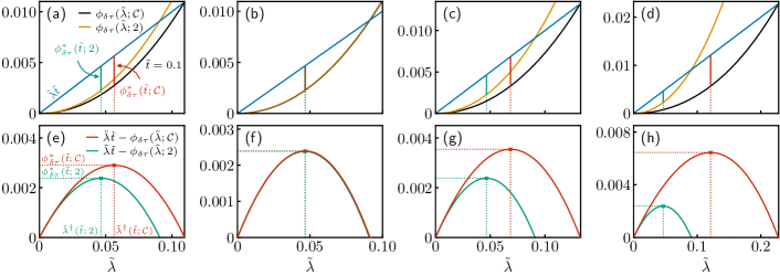
Figure S2: Illustration of the Cramér-Chernoff bounding method for the right tail with $\tilde{t}=0.1$ and parameters for spatially confined Brownian search process in dimensions $d=1$ (a,e) or $d=3$ (b,f), and discrete-state Markov jump processes for the model of calmodulin (c,d) and a 8-state toy protein (d,h). Top row depicts bounds of the cumulant generating function $\phi_{\delta\tau}(\tilde{\lambda};\mathcal{C})$ (black) and $\phi_{\delta\tau}(\tilde{\lambda};2)$ (yellow) as a function of $\tilde{\lambda}$, respectively. Bottom row shows the differences $\tilde{\lambda}\tilde{t}-\phi_{\delta\tau}(\tilde{\lambda};\mathcal{C})$ (red) and $\tilde{\lambda}\tilde{t}-\phi_{\delta\tau}(\tilde{\lambda};2)$ (green) as a function of $\tilde{\lambda}$, respectively (see also top row with $\tilde{\lambda}\tilde{t}$ in blue). The corresponding suprema are obtained at $\tilde{\lambda}^{\dagger}(\tilde{t};\mathcal{C})$ and $\tilde{\lambda}^{\dagger}(\tilde{t};2)$ (dotted lines) and define the Cramér transforms $\phi_{\delta\tau}^{*}(\tilde{t};\mathcal{C})$ and $\phi_{\delta\tau}^{*}(\tilde{t};2)$ (compare top row). For all considered models we demonstrate $\phi_{\delta\tau}(\tilde{\lambda};\mathcal{C})\leq\phi_{\delta\tau}(\tilde{\lambda};2)$ and $\phi_{\delta\tau}^{*}(\tilde{t};\mathcal{C})\geq\phi_{\delta\tau}^{*}(\tilde{t};2)$ as derived in the maintext. Note for the panels (b,f) we have $\phi_{\delta\tau}(\tilde{\lambda};\mathcal{C})\lessapprox\phi_{\delta\tau}(\tilde{\lambda};2)$ and $\phi_{\delta\tau}^{*}(\tilde{t};\mathcal{C})\gtrapprox\phi_{\delta\tau}^{*}(\tilde{t};2)$ since $\mathcal{C}=1.99\approx 2$.

S4.2 Theorem 2: Cramér-Chernoff bound for the left tail $\tau<\langle\tau\rangle$

Next we turn to the left tail, $\tau<\langle\tau\rangle$, where the corresponding moment generating function analogously reads

$$\langle{\rm e}^{\lambda(\langle\tau\rangle-\tau)}\rangle={\rm e}^{\lambda\langle\tau\rangle}\sum_{k>0}\frac{w_{k}}{1+\lambda/\mu_{k}}\leq\exp\left(\lambda\langle\tau\rangle+\sum_{k>0}\frac{{w}_{k}}{1+\lambda/\mu_{k}}-1\right)$$ (S18)

for $\lambda<\mu_{k}$. Using equivalent arguments as for the right tail above we may further write

$$\langle{\rm e}^{\lambda(\langle\tau\rangle-\tau)}\rangle \leq\exp\left(\sum_{m\geq 2}(-\lambda)^{m}\sum_{k>0}\frac{w_{k}}{\mu_{k}^{m}}\right)$$

$$=\exp\left(\lambda^{2}\frac{\langle\tau^{2}\rangle}{2}+\sum_{m>2}(-\lambda)^{m}\sum_{k>0}\frac{{w}_{k}}{\mu_{k}^{m}}\right)$$

$$\leq\exp\left(\lambda^{2}\frac{\langle\tau^{2}\rangle}{2}+\sum_{m>0}\frac{\lambda^{2m}}{\mu_{1}^{2m-2}}\sum_{k>0}\frac{{w}_{k}}{\mu_{k}^{2}}\right)=\exp\left(\lambda^{2}\frac{\langle\tau^{2}\rangle/2}{1-(\lambda/\mu_{1})^{2}}\right).$$ (S19)

Recall the definition of the cumulant generating function, $\psi_{\delta\tau}(\lambda)\equiv\ln\langle{\rm e}^{\lambda\delta\tau}\rangle$, such that Eq. (S19) directly yields

$$\psi_{\delta\tau}(\lambda)\leq\frac{\lambda^{2}}{2}\frac{\langle\tau^{2}\rangle}{1-(\lambda/\mu_{1})^{2}}=\frac{\tilde{\lambda}^{2}}{2}\frac{\mathcal{C}}{1-\tilde{\lambda}^{2}}\equiv\phi_{\delta\tau}(\tilde{\lambda};\mathcal{C})$$ (S20)

which completes the derivation of the lower expression in Eq. (6) of the Letter. Note that for the left tail we have $\delta\tau=\langle\tau\rangle-\tau$ and we again let $\tilde{t}\equiv\mu_{1}t$, $\tilde{\lambda}\equiv\lambda/\mu_{1}$, and $\mathcal{C}\equiv\mu_{1}^{2}\langle\tau^{2}\rangle$. In the case of general initial conditions $p_{0}(x_{0})\neq\tilde{p}_{\rm eq}(x_{0})$ we must simply again replace $\mathcal{C}\to 2\sum_{i}w_{i}\mathbbm{1}_{w_{i}>0}(\mu_{1}/\mu_{i})^{2}$ (see Lemma 2).

Analogous to the right tail we next compute the Cramér transform of Eq. (S20), i.e.,

$$\phi_{\delta\tau}^{*}(\tilde{t};\mathcal{C})\equiv\sup_{\tilde{\lambda}\in[0,1)}[\tilde{\lambda}\tilde{t}-\phi_{\delta\tau}(\tilde{\lambda};\mathcal{C})]=\sup_{\tilde{\lambda}\in[0,1)}\left[\tilde{\lambda}\tilde{t}-\frac{\tilde{\lambda}^{2}}{2}\frac{\mathcal{C}}{1-\tilde{\lambda}^{2}}\right],$$ (S21)

where we find the optimal value $\tilde{\lambda}^{\dagger}(\tilde{t};\mathcal{C})$ to be determined by the transcendental quartic, $\tilde{\lambda}^{\dagger}(\tilde{t}):(1-\tilde{\lambda}^{2})^{2}-\mathcal{C}_{\tilde{t}}\tilde{\lambda}=0$ with $\mathcal{C}_{\tilde{t}}\equiv\mathcal{C}/\tilde{t}$, which we solve according to the method of Descartes. First, we re-arrange the quartic as $\tilde{\lambda}^{4}-2\tilde{\lambda}^{2}-\mathcal{C}_{\tilde{t}}\tilde{\lambda}+1=0$ and make the factorization ansatz

$$(\tilde{\lambda}^{2}-y_{\tilde{t}}\tilde{\lambda}^{2}+w_{\tilde{t}})(\tilde{\lambda}^{2}+y_{\tilde{t}}\tilde{\lambda}^{2}+z_{\tilde{t}})=0$$

$$w_{\tilde{t}}+z_{\tilde{t}}-y_{\tilde{t}}^{2}=-2$$

$$y_{\tilde{t}}(w_{\tilde{t}}-z_{\tilde{t}})=-\mathcal{C}_{\tilde{t}}$$

$$z_{\tilde{t}}w_{\tilde{t}}=1.$$ (S22)

The system of equations (S22) is solved by

$$w_{\tilde{t}}(y_{\tilde{t}}) =(y_{\tilde{t}}^{2}-2-\mathcal{C}_{\tilde{t}}/y_{\tilde{t}})/2,$$

$$\quad z_{\tilde{t}}(y_{\tilde{t}}) =(y_{\tilde{t}}^{2}-2+\mathcal{C}_{\tilde{t}}/y_{\tilde{t}})/2,$$ (S23)

where $y_{\tilde{t}}^{2}\equiv Y_{\tilde{t}}$ is the solution of the cubic $Y_{\tilde{t}}^{3}-4Y_{\tilde{t}}^{2}-\mathcal{C}_{\tilde{t}}^{2}=0$. Moreover, since the discriminant $\mathrm{D}$ is strictly negative, i.e. $\mathrm{D}=-2^{8}\mathcal{C}_{\tilde{t}}^{2}-3^{3}\mathcal{C}_{\tilde{t}}^{4}<0$, the qubic has only one real root. The corresponding depressed qubic reads $\tilde{t}^{3}-2^{4}/3\tilde{t}-(2^{7}/3^{3}+\mathcal{C}_{\tilde{t}}^{2})=0$ with $\tilde{t}Y_{\tilde{t}}-4/3$. Let $p=-2^{4}/3<0$ and $q=-(2^{7}/3^{3}+\mathcal{C}_{\tilde{t}}^{2})<0$ then $2^{2}p^{3}+3^{3}q^{2}=-2^{12}/3^{3}+3^{3}(2^{7}/3^{3}+\mathcal{C}_{\tilde{t}}^{2})^{2}>0$ for any $\tilde{t}\geq 0$. We can express the unique real root as

$$y_{\tilde{t}}^{2}=\frac{4}{3}\left\{1+2\cosh\left[\frac{1}{3}{\rm arcosh}\left(1+\frac{3^{3}\mathcal{C}_{\tilde{t}}^{2}}{2^{7}}\right)\right]\right\}$$ (S24)

and $y=\pm\sqrt{y^{2}}$ with $y^{2}$ from Eq. (S24) can now be plugged into Eqs. (S23) to obtain $w_{\tilde{t}}(y)$ and $z_{\tilde{t}}(y)$ that are required to solve the pair of quadratic equations (S22). The four roots of the transcendental quartic are hence given by

$$\tilde{\lambda}_{1}(\tilde{t}) =\frac{y_{\tilde{t}}}{2}\left(1+\sqrt{1-4w_{\tilde{t}}(y_{\tilde{t}})/y_{\tilde{t}}^{2}}\right),$$

$$\tilde{\lambda}_{2}(\tilde{t}) =\frac{y_{\tilde{t}}}{2}\left(1-\sqrt{1-4w_{\tilde{t}}(y_{\tilde{t}})/y_{\tilde{t}}^{2}}\right),$$

$$\tilde{\lambda}_{3}(\tilde{t}) =-\frac{y_{\tilde{t}}}{2}\left(1-\sqrt{1-4z_{\tilde{t}}(y_{\tilde{t}})/y_{\tilde{t}}^{2}}\right),$$

$$\tilde{\lambda}_{4}(\tilde{t}) =-\frac{y_{\tilde{t}}}{2}\left(1+\sqrt{1-4z_{\tilde{t}}(y_{\tilde{t}})/y_{\tilde{t}}^{2}}\right).$$ (S25)

Moreover, we find $w_{\tilde{t}}(y_{\tilde{t}})/y_{\tilde{t}}^{2}=(1-2/y_{\tilde{t}}^{2}-\mathcal{C}_{\tilde{t}}/y_{\tilde{t}}^{3})/2$ and $z_{\tilde{t}}(y_{\tilde{t}})/y_{\tilde{t}}^{2}=(1-2/y_{\tilde{t}}^{2}+\mathcal{C}_{\tilde{t}}/y_{\tilde{t}}^{3})/2$. Since $y_{\tilde{t}}>0$ while $\tilde{\lambda}\in[0,1)$, $\tilde{\lambda}_{2},\tilde{\lambda}_{3}$ in Eq. (S25) are excluded automatically (note also that the square root in $\tilde{\lambda}_{2},\tilde{\lambda}_{3}$ becomes complex for $\tilde{t}\to\infty$). We also have $\lim_{\tilde{t}\to\infty}y_{\tilde{t}}^{2}=4$ and $\lim_{\tilde{t}\to\infty}w_{\tilde{t}}(y_{\tilde{t}})=1$ such that $\lim_{\tilde{t}\to\infty}\tilde{\lambda}_{1}=\tilde{\lambda}_{2}=1$. Conversely, we find that $\lim_{\tilde{t}\to 0}\tilde{t}^{2/3}y_{\tilde{t}}^{2}=\mathcal{C}^{2/3}=\lim_{\tilde{t}\to 0}\tilde{t}^{2/3}\mathcal{C}_{\tilde{t}}/y_{\tilde{t}}$ such that $\lim_{\tilde{t}\to 0}w_{\tilde{t}}(y_{\tilde{t}})=-1$ while $\lim_{\tilde{t}\to 0}w_{\tilde{t}}(y_{\tilde{t}})y_{\tilde{t}}^{2}=-{\mathcal{C}_{\tilde{t}}}^{2/3}=0$. Therefore, $\lim_{\tilde{t}\to 0}\tilde{\lambda}_{1}=y_{\tilde{t}}\to\infty$ whereas $\lim_{\tilde{t}\to 0}\tilde{\lambda}_{2}(\tilde{t})=y_{\tilde{t}}\times 0/2\searrow 0$. We recall that $\tilde{\lambda}\in[0,1)$ which therefore excludes $\tilde{\lambda}_{1}(\tilde{t})$ and identifies $\tilde{\lambda}^{\dagger}(\tilde{t})=\tilde{\lambda}_{2}(\tilde{t})$ as the supremum. Finally, we introduce the auxiliary functions

$$g(u)\equiv\frac{2}{\sqrt{3}}\left\{1+2\cosh\left[\frac{1}{3}{\rm arcosh}\left(1+\frac{3^{3}}{2^{7}u^{2}}\right)\right]\right\}^{1/2}\quad\text{and}\quad\Lambda(u)\equiv\frac{1}{2}\left[g(u)-\sqrt{4+2/g(u)u-g(u)^{2}}\right],$$ (S26)

as well as

$$h_{-}(u)\equiv\Lambda(u)u-\frac{1}{2}\frac{\Lambda(u)^{2}}{1-\Lambda(u)^{2}}$$ (S27)

which allows us to obtain and write the Cramér transform as

$$\phi_{\delta\tau}^{*}(\tilde{t};\mathcal{C})=\mathcal{C}h_{-}(\tilde{t}/\mathcal{C})=\mathcal{C}h_{-}(\mu_{1}t/\mathcal{C}),\quad 0\leq t\leq\langle\tau\rangle.$$ (S28)

In the last step we use Chernoff’s inequality to obtain the bound $\mathbbm{P}(\delta\overline{\tau}_{n}\geq t)\leq{\rm e}^{-n\phi^{*}_{\delta\tau}(t;\mathcal{C})}\equiv\mathcal{U}^{-}_{n}(t;\mathcal{C})$ for $0\leq t\leq\langle\tau\rangle$ which completes the proof of Theorem 2 and hence the derivation of the lower expression in Eq. (7) of the Letter.

Figure S3: Illustration of the Cramér-Chernoff bounding method for the left tail with $\tilde{t}=0.1$ and parameters for spatially confined Brownian search process in dimensions $d=1$ (a,e) or $d=3$ (b,f), and discrete-state Markov jump processes for the model of calmodulin (c,d) and a 8-state toy protein (d,h). Top row depicts bounds of the cumulant generating function $\phi_{\delta\tau}(\tilde{\lambda};\mathcal{C})$ (black) and $\phi_{\delta\tau}(\tilde{\lambda};2)$ (yellow) as a function of $\tilde{\lambda}$, respectively. Bottom row shows the differences $\tilde{\lambda}\tilde{t}-\phi_{\delta\tau}(\tilde{\lambda};\mathcal{C})$ (red) and $\tilde{\lambda}\tilde{t}-\phi_{\delta\tau}(\tilde{\lambda};2)$ (green) as a function of $\tilde{\lambda}$, respectively (see also top row with $\tilde{\lambda}\tilde{t}$ in blue). The corresponding suprema are obtained at $\tilde{\lambda}^{\dagger}(\tilde{t};\mathcal{C})$ and $\tilde{\lambda}^{\dagger}(\tilde{t};2)$ (dotted lines) and define the Cramér transforms $\phi_{\delta\tau}^{*}(\tilde{t};\mathcal{C})$ and $\phi_{\delta\tau}^{*}(\tilde{t};2)$ (compare top row). For all considered models we demonstrate $\phi_{\delta\tau}(\tilde{\lambda};\mathcal{C})\leq\phi_{\delta\tau}(\tilde{\lambda};2)$ and $\phi_{\delta\tau}^{*}(\tilde{t};\mathcal{C})\geq\phi_{\delta\tau}^{*}(\tilde{t};2)$ as derived in the maintext. Note for the panels (b,f) we have $\phi_{\delta\tau}(\tilde{\lambda};\mathcal{C})\lessapprox\phi_{\delta\tau}(\tilde{\lambda};2)$ and $\phi_{\delta\tau}^{*}(\tilde{t};\mathcal{C})\gtrapprox\phi_{\delta\tau}^{*}(\tilde{t};2)$ since $\mathcal{C}=1.99\approx 2$.

S4.3 Behavior of upper bounds $\mathcal{U}^{\pm}_{n}(t)$ for large sample sizes

Here, we present some further remarks about the limit of large sample sizes. Asymptotically as $n\to\infty$, $\mathcal{U}^{\pm}_{n}(t)$ is substantial only for $\tilde{t}/\mathcal{C}\ll 1$. For the right tail bound $h_{+}(u)$ we immediately find that for $u\ll 1$ we can Taylor expand $\sqrt{1+2u}=1+u-u^{2}/2+\mathcal{O}(u^{3})$. Consequently we directly obtain $h_{+}(u)=u^{2}/2-\mathcal{O}(u^{3})$, i.e., the upper tail is sub-Gaussian for small deviations and will converge to a Gaussian as $n\to\infty$. For the left tail we furthermore have ${\rm arcosh}(1+x)=\ln(1+x+\sqrt{x(x+2)})$ and thus $\lim_{x\to\infty}{\rm arcosh}(1+x)=\ln(2x)-1/(2x)^{2}$. As a result it follows that $\frac{1}{3}\lim_{u\to 0}{\rm arcosh}(1+3^{3}/2^{7}u^{2})\simeq\frac{1}{3}\ln(3^{3}/2^{6}u^{2})=\ln(3/4u^{2/3})-u^{4}2^{12}/3^{7}$ and thus

$$\lim_{u\to 0}g(u) \simeq\frac{2}{\sqrt{3}}\{1+2\cosh\ln(3/4u^{2/3})\}^{1/2}=\frac{2}{\sqrt{3}}[1+3/4u^{2/3}]^{1/2}$$ (S29)

$$=u^{-1/3}[1+4u^{2/3}/3]^{1/2}=u^{-1/3}[1+2u^{2/3}/3+\mathcal{O}(u^{4/3})]=u^{-1/3}+\frac{2}{3}u^{1/3}+\mathcal{O}(u).$$ (S30)

A lengthy but straightforward calculation subsequently reveals that $\lim_{u\to 0}\Lambda(u)=u-\mathcal{O}(u^{3})$ such that

$$\lim_{u\to 0}\frac{\Lambda(u)^{2}}{1-\Lambda(u)^{2}}\simeq\frac{u^{2}}{1-u^{2}}=u^{2}+\mathcal{O}(u^{4}).$$ (S31)

We therefore have that $\lim_{u\to 0}h_{-}(u)=u^{2}/2-\mathcal{O}(u^{4})$, i.e., both tails are sub-Gaussian for $\tilde{t}/\mathcal{C}\ll 1$ with $\mathcal{C}\equiv\mu_{1}^{2}\langle\tau^{2}\rangle$.

S4.4 Proof of bounds on $\mathcal{C}$ and model-free concentration inequalities

Notably, system details only enter the Cramér transforms (S17) and (S28) (and consequently upper bounds on the deviation probability due to Chernoff’s inequality) in the form of a system-specific constant $\mathcal{C}\equiv\mu_{1}^{2}\langle\tau^{2}\rangle$. Note that here we only allow for equilibrium initial conditions. Recalling that the moments of the first-passage time $\tau$ are expressed as $\langle\tau^{m}\rangle=m!\sum_{k>0}w_{k}/\mu_{k}^{m}$ allows us to write

$$0\leq 2\frac{w_{1}}{\mu_{1}^{2}}\leq\langle\tau^{2}\rangle=2\sum_{k>0}\frac{w_{k}}{\mu_{k}^{2}}\leq 2\sum_{k>0}\frac{w_{k}}{\mu_{1}^{2}}=\frac{2}{\mu_{1}^{2}}$$ (S32)

where we have used that $w_{k}$ are non-negative, normalized, and $\mu_{1}\leq\mu_{k>1}$. Consequently, by Eq. (S32), we immediately find that the system-constant itself is bounded $0\leq 2w_{1}\leq\mathcal{C}\leq 2$. Note that analogous considerations can be used to more generally obtain $0\leq m!w_{1}\leq\mu_{1}^{m}\langle\tau^{m}\rangle\leq m!$ for the $m$-th moment, i.e., for $m=1$ we find the chain of inequalities $0\leq w_{1}\leq\mu_{1}\langle\tau\rangle\leq 1$.

The fact that $\mathcal{C}\in(0,2]$ can now be further leveraged to arrive at the model-free bounds (Eq. (11) in the Letter) which require no information about the underlying system. Recall the upper bounds of the cumulant generating function $\phi_{\delta\tau}(\tilde{\lambda};\mathcal{C})$ and their corresponding Cramér transform $\phi_{\delta\tau}^{*}(\tilde{t};\mathcal{C})$, i.e.,

$$\phi_{\delta\tau}(\tilde{\lambda};\mathcal{C})=\begin{dcases}\frac{\tilde{\lambda}^{2}}{2}\frac{\mathcal{C}}{1-\tilde{\lambda}}&\tau\geq\langle\tau\rangle\\ \frac{\tilde{\lambda}^{2}}{2}\frac{\mathcal{C}}{1-\tilde{\lambda}^{2}}&\tau<\langle\tau\rangle,\end{dcases}\qquad\text{and}\qquad\phi_{\delta\tau}^{*}(\tilde{t};\mathcal{C})=\begin{dcases}\mathcal{C}h_{+}(\tilde{t}/\mathcal{C})&\tau\geq\langle\tau\rangle\\ \mathcal{C}h_{-}(\tilde{t}/\mathcal{C})&\tau<\langle\tau\rangle.\end{dcases}$$ (S33)

Since $\phi_{\delta\tau}(\tilde{\lambda};\mathcal{C})$ is monotonically increasing in $\mathcal{C}$ it follows that $\phi_{\delta\tau}(\tilde{\lambda};\mathcal{C})\leq\phi_{\delta\tau}(\tilde{\lambda};2)$, $\forall\tilde{\lambda}\in[0,1)$ (see Figs S2 and S3 top row). By definition of $\phi_{\delta\tau}^{*}(\tilde{t};\mathcal{C})\equiv\sup_{\tilde{\lambda}\in[0,1)}(\tilde{\lambda}\tilde{t}-\phi_{\delta\tau}(\tilde{\lambda};\mathcal{C}))$ this bound in turn implies that $\phi_{\delta\tau}^{*}(\tilde{t};\mathcal{C})\geq\phi_{\delta\tau}^{*}(\tilde{t};2)$ (compare Figs. S2 and S3 bottom row). With Chernoff’s inequality we moreover arrive at $\mathbbm{P}(\delta\overline{\tau}_{n}\geq t)\leq{\rm e}^{-n\phi^{*}_{\delta\tau}(t;\mathcal{C})}\leq{\rm e}^{-n\phi^{*}_{\delta\tau}(t;2)}$ and hence $\mathcal{U}^{\pm}_{n}(t;\mathcal{C})\leq\mathcal{U}^{\pm}_{n}(t;2)$ which completes the derivation of Eq. (11) in the Letter.

S5 Model systems and details on numerical methods

In the Letter we exemplify our results by considering a Brownian molecular search process in dimensions $d=1$ and $d=3$, as well as discrete-state Markov-jump models of protein folding for a 8-state toy protein and the experimentally inferred model of calmodulin (compare Fig. 1b-d). In this section we present further details on the model systems and their numerical treatment.

S5.1 Continuous-time discrete-state Markov jump process

As illustrative discrete-state continuous-time Markov-jump models of protein folding we consider a simple 8-state toy protein [11, 38] and further use the experimentally inferred folding network of the cellular calcium sensor protein calmodulin [42]. Since we consider equilibrium initial conditions, proteins start from an initial state drawn from the equilibrium density $\tilde{p}_{\rm eq}(x_{0})$—note that the tilde denotes that the absorbing target is excluded—from which they search the native state $a$ (here $a=(1,1,1)$ for the 8-state model and $a=F_{1234}$ for calmodulin; cf. Fig. 1b-d). Arrows in the networks denote possible transitions, e.g. a transition from state $i$ to state $j$ that occurs with the corresponding rate $L_{ji}$. We consider reversible dynamics, i.e., the resulting transition matrix $\hat{L}$ of the relaxation process satisfies detailed balance $p_{\rm eq,\textit{j}}/p_{\rm eq,\textit{i}}=L_{ji}/L_{ij}=\exp(F_{i}-F_{j})$ and transitions rates are connected to the free energy of the states $F_{i}$ [43].

We recall that the first-passage time density $\wp_{a}(t)$ can be evaluated by using the spectral representation (S1). To this end we set up the modified transition matrix, adopting in this section the Dirac bra-ket notation, $\hat{L}_{a}=\hat{L}-|a\rangle\langle a|$ where $|a\rangle\equiv(0,\ldots,0,1,0,\ldots)^{\intercal}$ defines a vector with all entries zero expect at the $a$-th position of the absorbing state where it equals one. This effectively removes all transitions that correspond to jumps leaving the absorbing state $a$. Next, we carry out an eigendecomposition of $\hat{L}_{a}$ and determine the eigenvalues $\mu_{k}$, right eigenvectors $|\phi^{\rm R}\rangle$, and left eigenvectors $\langle\phi^{\rm L}|$. We subsequently use obtained eigenmodes to compute the first-passage weights $w_{k}(x_{0})=-\langle a|\phi_{k}^{\rm R}\rangle\langle\phi_{k}^{\rm L}|x_{0}\rangle$ (see [37, 38]), and recall that $\mu_{k}$ and $w_{k}$ determine the moments according to $\langle\tau^{m}\rangle=m!\sum_{k>0}w_{k}/\mu_{k}^{m}$. Corresponding relevant parameters of the Markov jump models are listed in Tab. 1. Next we give further details on how matching transition rates are constructed.

Table 1: Parameters for the Markov jump models for the 8-state toy protein and the inferred model of calmodulin. Listed are values for the first-passage eigenvalues $\mu_{k}$, first-passage weights $w_{k}$, and the first $\langle\tau\rangle$ and second moment $\langle\tau^{2}\rangle$.

Model	$\mu_{1}$	$w_{1}$	$\mu_{2}$	$w_{2}$	$\mu_{3}$	$w_{3}$	$\mu_{4}$	$w_{4}$	$\mu_{5}$	$w_{5}$	$\mu_{6}$	$w_{6}$	$\mu_{7}$	$w_{7}$	$\langle\tau\rangle$	$\langle\tau^{2}\rangle$
Toy protein	0.976	0.337	6.148	0.009	1.551	0.583	4.203	0.001	4.396	0.0001	6.233	0.060	12.834	0.010	0.385	0.713
Calmodulin	0.469	0.651	3.763	0.349	19.097	9.98E-5	143.749	2.42E-9	1581.629	1.52E-6	–	–	–	–	1.479	5.958

S5.1.1 Transitions rates of the 8-state toy protein model

For the 8-state toy protein model we randomly generate a free energy level $F_{i}$ for each state $i\in\{1,2,3,4,5,6,7,8\}$ with $F_{i}$ uniformly distributed within the interval $0\leq F_{i}\leq 10$. Transition rates that satisfy detailed balance are then obtained using the ansatz

$$k_{i\to j}\equiv L_{ji}=\exp(\Delta F_{i}/2)\qquad\text{and}\qquad k_{j\to i}\equiv L_{ij}=\exp(-\Delta F_{i}/2),$$ (S34)

where $\Delta F_{i}\equiv F_{i}-F_{j}$ and thus $\ln(L_{ji}/L_{ij})=\Delta F_{i}=F_{i}-F_{j}$. Obtained individual transition rates are listed in Tab. 2.

Table 2: Transition rates for the 8-state toy protein model obtained via the ansatz described in the main text.

transition	rate $k_{i\to j}$	transition	rate $k_{i\to j}$	transition	rate $k_{i\to j}$	transition	rate $k_{i\to j}$
$1\to 2$	1.878	$2\to 5$	2.648	$3\to 7$	4.549	$5\to 8$	0.106
$2\to 1$	5.327	$5\to 2$	3.421	$7\to 3$	1.00994	$8\to 5$	124.477
$1\to 3$	0.00463	$2\to 6$	0.527	$4\to 6$	0.358	$6\to 8$	0.712
$3\to 1$	0.507	$6\to 2$	36.0577	$6\to 4$	36.457	$8\to 6$	15.794
$1\to 4$	0.326	$3\to 5$	1.109	$4\to 7$	0.523	$7\to 8$	0.322
$4\to 1$	0.623	$5\to 3$	0.0371	$7\to 4$	6.670	$8\to 7$	56.998

S5.1.2 Transitions rates of the calmodulin protein model

In the experimental setup a constant external force $f$, a so-called pretension, is applied to the calmodulin protein via optical tweezers [42]. Folding and unfolding processes are observed at different pretensions ranging from $6\,\text{pN}$ to $13\,\text{pN}$ and corresponding force-dependent transition rates $k_{i\to j}(f)=L_{ji}(f)$ between two conformational states $i$ and $j$ are measured. Note that $i,j\in\{\text{Unfold},F_{12},F_{123},F_{23},F_{34},F_{1234}\}$ and we further map states according to $\text{Unfold}\leftrightarrow 1$, $F_{12}\leftrightarrow 2$, $F_{123}\leftrightarrow 3$, $F_{23}\leftrightarrow 4$, $F_{34}\leftrightarrow 5$, and $F_{1234}\leftrightarrow 6$ for convenience. For our purposes we choose, without loss of generality, a pretension of $f=9\,\text{pN}$ and obtain the corresponding measured transitions rates from Fig. S8 in the Supplementary Material of [42]. Clearly, experimental transitions rates are accompanied with measurement uncertainties which is reflected in slight “deviations” from a mathematically precise definition of detailed balance. To mitigate this issue, and to ensure that transition rates precisely obey detailed balance $k_{i\to j}p_{\rm eq,\textit{i}}=k_{j\to i}p_{\rm eq,\textit{j}}$, we further have to slightly adjust the rates.

First, we compute the invariant density $p_{\rm eq}$ from the experimental rates and obtain a corresponding free energy level $F_{i}=-\ln(p_{\rm eq,\textit{i}})$. Next, we use the ansatz (S34), i.e., $L_{ji}=A_{i}\exp(\Delta F_{i}/2)$ and $L_{ij}=A_{i}\exp(-\Delta F_{i}/2)$ where we introduce a constant $A_{i}$. Finally, $A_{i}$’s are chosen such that resulting transition rates fall within experimental error bars in Ref. [42]. Obtained transition rates are listed in Table 3.

Table 3: Transition rates of the Markov jump model for the calmodulin protein. Rates are extracted from the Supplemental Material of Ref. [42] and modified such that they obey detailed balance precisely according to the maintext.

transition	rate $k_{i\to j}$	transition	rate $k_{i\to j}$	transition	rate $k_{i\to j}$
$1\to 2$	5.997	$1\to 4$	13.439	$1\to 5$	15.330
$2\to 1$	0.774	$4\to 1$	127.968	$5\to 1$	0.121
$5\to 6$	3.749	$2\to 3$	1514.820	$2\to 6$	13.441
$6\to 5$	13.326	$3\to 2$	53.0661	$6\to 2$	2.922

S5.2 Spatially confined Brownian molecular search process

We also test our theory for Markov processes on a continuous state-space. More precisely, we consider the spatially confined diffusive search of a Brownian particle in a $d$-dimensional unit sphere with a reflecting boundary at $R=1$ and a perfectly absorbing spherical target of radius $0<a<1$, here $a=0.1$, in the center (compare Fig. 1b). The closest distance of the particle to the surface of the absorbing sphere at time $t$ is a confined Bessel process (see e.g. [44, 45, 38]) which time evolution obeys the Itô equation

$$dx_{t}=(d-1)x_{t}^{-1}dt+\sqrt{2}dW_{t},$$ (S35)

where $dW_{t}$ is the increment of a Wiener process (i.e. Gaussian white noise) with $\langle dW_{t}\rangle=0$ and $\langle dW_{t}dW_{t^{\prime}}\rangle=\delta(t-t^{\prime})dt$, and we have set, without loss of generality, $D=1$. The general case with any $0<D<\infty$ and a sphere of radius $R$ is covered by expressing time in units of $R^{2}/D$.

For $d=1$ Eq. (S35) reduces to a $1$ dimensional Brownian motion which has the equilibrium first-passage weights

$$w_{k}^{\rm eq}=\frac{2}{\pi^{2}}\frac{1-\sin\left[(k-1)\pi\right]}{(k-1/2)^{2}}$$ (S36)

and matching first-passage eigenvalues are obtained as $\mu_{k}=\pi^{2}(k-1/2)^{2}$. Moreover, for $d=3$ the first-passage time probability density of the Bessel process can be evaluated exactly and has the equilibrium weights

$$w_{k}^{\rm eq}=\frac{2}{\mu_{k}}\frac{3a^{2}}{1-a^{3}}\frac{\tan[(1-a)\sqrt{\mu_{k}}]+\frac{1}{\sqrt{\mu_{k}}}}{(1-a)\tan[(1-a)\sqrt{\mu_{k}}]-\frac{a}{\sqrt{\mu_{k}}}},$$ (S37)

with the first-passage eigenvalues $\mu_{k}$ being the solutions of the transcendental equation $\sqrt{\mu_{k}}=\tan([1-a]\sqrt{\mu_{k}})$ that can be solved analytically using Newton’s series [38]. Relevant parameters for the spatially confined Brownian search process with $a=0.1$ are listed in Tab. LABEL:SM_Tab_Bessel.

Note that the mean for $d=3$ and arbitrary $x_{0}$ can be obtained directly [46] as $\langle\tau_{a}(x_{0})\rangle=[1/a-1/x+a^{2}/2-x^{2}/2]/3$ which integrated over all starting positions, i.e. equilibrium initial conditions, gives the global mean first-passage time

$$\langle\tau_{a}^{\rm eq}\rangle=\left[\frac{4\pi}{3}(1-a^{3})\right]^{-1}\int_{a}^{1}\frac{4\pi}{3}\left[\frac{1}{a}-\frac{1}{x}+\frac{a^{2}}{2}-\frac{x^{2}}{2}\right]dx=\frac{1}{1-a^{3}}\left[\frac{1-a^{3}}{3a}-\frac{1-a^{2}}{2}+\frac{a^{2}(1-a^{3})}{6}-\frac{1-a^{5}}{10}\right].$$ (S38)

Table 4: Parameters for the spatially confined Brownian molecular search process in dimensions $1$ and $3$. Listed are values for the first $5$ first-passage eigenvalues $\mu_{k}$, first-passage weights $w_{k}$, and the first $\langle\tau\rangle$ and second moment $\langle\tau^{2}\rangle$, respectively .

Model	$\mu_{1}$	$w_{1}$	$\mu_{2}$	$w_{2}$	$\mu_{3}$	$w_{3}$	$\mu_{4}$	$w_{4}$	$\mu_{5}$	$w_{5}$	$\langle\tau\rangle$	$\langle\tau^{2}\rangle$
1D Brownian motion	2.467	0.811	22.207	0.0901	61.685	0.0324	120.903	0.0165	199.859	0.01001	0.333	0.267
3D Bessel process	0.363	0.994	25.174	0.00277	73.926	9.163E-4	147.037	4.573E-4	244.516	2.742E-4	2.739	15.09

S5.3 Statistics of first-passage times $\tau$, the sample mean $\overline{\tau}_{n}$, maximum $\tau^{+}_{n}$, and minimum $\tau^{-}_{n}$

Finally we provide some further details on the sampling method used to obtain the statistics of (i) the first-passage time $\tau$, (ii) the sample-mean $\overline{\tau}_{n}\equiv\sum_{i}\tau_{i}/n$, and (iii) the expected maximal and minimal deviation from the mean $\langle\tau^{\pm}_{n}-\langle\tau\rangle\rangle$ for a sample with a fixed number $n$ of independent realizations for all considered models.

We recall that after determining the first-passage eigenvalues $\mu_{k}$ and first-passage weights $w_{k}$, the first-passage time density $\wp_{a}(t)$ (S1) and survival probability $S_{a}(t)$ (S2) are fully characterized. To now sample the random variable $\tau$, i.e. individual realizations of the first-passage process, we employ the so-called inversion sampling method [47]. This method allows us to generate independent samples of $\tau$ from $\wp_{a}(t)$ given its cumulative distribution function (CDF) which is directly related to the survival probability according to $1-S_{a}(t)$. Note that for discrete-state dynamics the number of states $M$ is finite, i.e. $k=1,\ldots,M$, and therefore Eq. (S2) (and hence the CDF) is a finite sum. In contrast, for continuous-state dynamics we formally have $M=\infty$, meaning that sums are here not finite. For the following numerical evaluation of the spatially confined Brownian search process we therefore truncate the sum after $M=1000$ terms. The first-passage time densities $\wp_{a}(t)$ obtained via inversion sampling (symbols) for all considered models are shown in Fig. S4a-d and corroborated by the corresponding analytical result (S1) (dashed black line).

For Fig. 2a-d in the Letter empirical probabilities that ${\overline{\tau}_{n}-\langle\tau\rangle}$ lies within a desired range of $\pm$ 10% of the longest first-passage time scale $\mu_{1}^{-1}$, $\mathbbm{P}(\mu_{1}[\overline{\tau}_{n}-\langle\tau\rangle]\in[-0.1,0.1])$, are computed using statistics of the sample mean $\overline{\tau}_{n}$ by fixing $n$, i.e., the number of individual realizations the average is taken over. In particular, we have $n\in\{1,2,3,5,10,20,30,40,50,75,100,150,200,300,400,500\}$. Subsequently, for each individual fixed $n$ the sample mean $\overline{\tau}_{n}$ itself is sampled a total of $N=10^{6}$ times. That is, we first draw $n$ first-passage times $\tau$, compute $\overline{\tau}_{n}$ by averaging over the drawn $n$ realizations, and finally repeat this step $N=10^{6}$ times to obtain statistics of $\overline{\tau}_{n}$ for all $n$ values introduced above. Probability densities of the sample mean are shown in Fig. S4e-h for $n\in\{3,5,10,20\}$ and all model systems. Corresponding true mean first-passage times $\langle\tau\rangle$ are highlighted in grey.

In Fig. 2e-h of the Letter the probabilities to deviate more than $t$ in either direction, $\mathbbm{P}(\pm[\overline{\tau}_{n}-\langle\tau\rangle]\geq t)$, are computed from analogous statistics of the sample mean $\overline{\tau}_{n}$. Since we also consider empirical probabilities for rare events with large deviations (i.e. large $\mu_{1}t$) we however require substantially more statistics of $\overline{\tau}_{n}$. To this end we now have $N=10^{7}$ for $n\in\{1,3\}$ and $N=10^{11}$ for $n\in\{5,10,20\}$. In addition it should be further noted that we re-scale obtained probabilities according to $\mathbbm{P}^{1/n}$. To compute an empirical deviation probability where e.g. $\mathbbm{P}^{1/20}=0.1$ one would be thus required to sample rare events that occur with a probability of $\simeq 10^{-20}$.

In Fig. 3a of the Letter each data point corresponds to the relative error $\mu_{1}(\overline{\tau}_{n}-\langle\tau\rangle)$ (note that $\mu_{1}$ and $\langle\tau\rangle$ are different for each model) where the sample mean $\overline{\tau}_{n}$ is again obtained by first fixing $n$ and then sampling $n$ first-passage times $\tau$ according to the inversion sampling method and subsequently taking the average.

In Fig. 3d-e in the Letter and Figs. S6 and S7 below we show the expected deviation of the maximum $\tau^{+}_{n}$ and minimum $\tau^{-}_{n}$ in a sample of $n$ realizations from the mean first-passage time $\langle\tau\rangle$ as a function of $\mu_{1}\langle\tau\rangle$. To sample values over the entire range of possible values $\mu_{1}\langle\tau\rangle\in[0,1]$ we generate $10000$ random folding landscapes for the Markov jump process network of Calmodulin and the 8-state toy protein model, respectively. Each data point shown corresponds to one particular realization of the Markov jump process for the given network topology where transitions rates obeying detailed balance are constructed using the methods described in Sec. S5.1. The free energy levels $F_{i}$ are now uniformly distributed within the interval $0\leq F_{i}\leq 20$. For each random realization of a folding landscape (i.e., data point) we draw a fixed number of independent first-passage times $n\in\{3,5,10,20\}$ using inversion sampling to determine the minimum $\tau^{-}_{n}$ and maximum $\tau^{+}_{n}$, receptively. To compute the associated averages $\langle\tau^{\pm}_{n}\rangle$ we acquire minimal and maximal $\tau^{\pm}_{n}$’s for a total of $10^{7}$ independent draws of $n$ realizations for each of the $10000$ respective random folding landscapes. The same procedure is applied to the confined diffusion process where for $d=3$ we vary the target radius $a\in[0.05,0.95]$. Note that in the case of $d=1$ we have no parameter to vary, i.e., there is only one data point.

Figure S4: Inversion sampling of first-passage statistics for a confined Brownian search process in dimensions (a,e) $d=1$ and (b,f) $d=3$, and discrete-state Markov jump processes for (c,d) the calmodulin network and (d,h) a 8-state toy protein. (a-d) First-passage time density $\wp_{a}(t)$ obtained using inversion sampling (symbols) and analytical result as black dashed lines. (e-h) Empirical probability density of the sample mean $\overline{\tau}_{n}$ for different $n$ values. True mean first-passage times $\langle\tau\rangle$ are shown in grey.

S6 Uncertainty quantification with confidence intervals

In this section we extend the discussion and present some further details on the confidence intervals introduced in the Letter. Our derived upper bounds $\mathcal{U}^{\pm}_{n}(t)$ can be applied to construct non-asymptotic performance guarantees such as confidence intervals. In particular, they can be employed to bound the probability that $\delta\overline{\tau}_{n}\equiv\overline{\tau}_{n}-\langle\tau\rangle$ is found to be in some interval $[-t^{-}_{\alpha_{-}},t^{+}_{\alpha_{+}}]$, i.e.,

$$\mathbbm{P}(\delta\overline{\tau}_{n}\in[-t^{-}_{\alpha_{-}},t^{+}_{\alpha_{+}}]) =\mathbbm{P}(-t^{-}_{\alpha_{-}}\leq\delta\overline{\tau}_{n}\leq t^{+}_{\alpha_{+}})$$

$$=\mathbbm{P}(\delta\overline{\tau}_{n}\geq-t^{-}_{\alpha_{-}}\cap\delta\overline{\tau}_{n}\leq t^{+}_{\alpha_{+}})$$

$$\geq 1-\mathbbm{P}(\delta\overline{\tau}_{n}\leq-t^{-}_{\alpha_{-}})-\mathbbm{P}(\delta\overline{\tau}_{n}\geq t^{+}_{\alpha_{+}})$$

$$\geq 1-\underbrace{\mathcal{U}^{-}_{n}(t^{-}_{\alpha_{-}})}_{\equiv\alpha_{-}}-\underbrace{\mathcal{U}^{+}_{n}(t^{+}_{\alpha_{+}})}_{\equiv\alpha_{+}}.$$ (S39)

In passing from the second to the third line we have applied Boole’s second inequality, and from the third to forth line we use bounds (7) of the Letter. In the last line we additionally introduced acceptable right and left tail error probabilities $\alpha_{\pm}$. The implicit interval $[-t^{-}_{\alpha_{-}},t^{+}_{\alpha_{+}}]$ therefore defines a confidence interval at a confidence level of $1-\alpha$ with $\alpha\equiv\alpha_{+}+\alpha_{-}$, and $\alpha_{+}+\alpha_{-}<1$. In general the choice of the confidence interval for a fixed probability $1-\alpha$ is not unique. Some common options in the literature (see e.g. [48, 3]), all having the same confidence level, are listed below.

• One common choice are so-called central intervals (blue lines in Fig. S5) which correspond to equal tail probabilities $\alpha_{+}=\alpha_{-}=\alpha/2$ for the complementary intervals $[-\langle\tau\rangle,-t^{-}_{\alpha_{-}}]$ and $[t^{+}_{\alpha_{+}},\infty)$. Notably, we remark that central confidence intervals do not generally imply that $t^{+}_{\alpha_{+}}$ and $t^{-}_{\alpha_{-}}$ are equidistant from another, i.e., $t^{+}_{\alpha_{+}}\neq t^{-}_{\alpha_{-}}$.

• As an alternative one could likewise choose $t^{+}_{\alpha_{+}}=t^{-}_{\alpha_{-}}\equiv\Delta t/2$, which subsequently leads to the symmetric interval $[-\Delta t/2,\Delta t/2]$ with total length $\Delta t$ (see red lines in Fig. S5) . Analogously, a symmetric interval does not necessarily imply that the corresponding tail probabilities are equal, i.e., in general $\alpha_{+}\neq\alpha_{-}$.

• Both considerations above lead to two-sided intervals. However, another possible choice includes the fully asymmetric intervals $[-\langle\tau\rangle,t^{+}_{\alpha_{+}}]$ and $[-t^{-}_{\alpha_{-}},\infty)$, i.e., one-sided intervals with a corresponding confidence level $1-\alpha_{+}$ (for the upper limit $t^{+}_{\alpha_{+}}$) and $1-\alpha_{-}$ (for the lower limit $t^{-}_{\alpha_{-}}$), respectively,

  $$\mathbbm{P}(\pm\delta\overline{\tau}_{n}\leq t^{\pm}_{\alpha_{\pm}})\geq 1-\alpha_{\pm}.$$ (S40)

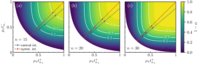
Figure S5: Contour plot of different choices of possible two-sided confidence intervals $[-\mu_{1}t^{-}_{\alpha_{-}},\mu_{1}t^{+}_{\alpha_{+}}]$ for a fixed confidence level $\alpha$ and (a) $n=15$, (b) $n=20$, (c) $n=30$. Contour lines for $\alpha\in\{0.1,0.3,0.5\}$ are depicted in white. Specific choices of central and symmetric are shown in blue and red, respectively, and we let $\mathcal{C}=1$ for all panels.

Confidence intervals are practically useful as they answer questions such as e.g.:

How many realizations are required to achieve a desired accuracy with a specified probability?
Or: For a given number of realizations a desired accuracy is achieved with at least what probability?

In the case of symmetric confidence intervals $t^{+}_{\alpha_{+}}=t^{-}_{\alpha_{-}}$ (see Fig. S5 red lines) the interval endpoints are implicitly defined via the last line of Eq. (S39) which is easily solved using standard root-finding procedures like the bi-section method [49]. The same holds true for other interval choices, however, when specifying the error probabilities $\alpha_{\pm}$ directly—as done for e.g. two-sided central intervals ($\alpha_{\pm}=\alpha/2$) or one-sided intervals—it suffices to solve Eq. (S40) with the respective $\alpha_{\pm}$. Hereby, the lower confidence limit $t^{-}_{\alpha_{-}}$ is again easily obtained using standard root-finding methods. Notably, the upper confidence limit $t^{+}_{\alpha_{+}}$ can now be solved analytically. To show this we consider $\mathcal{U}_{n}^{+}(t^{+}_{\alpha_{+}};\mathcal{C})=\alpha_{+}$, i.e., we identify the $t^{+}_{\alpha_{+}}$ that solves

$$0=-n\mathcal{C}h_{+}(\mu_{1}t^{+}_{\alpha_{+}}/\mathcal{C})-\ln(\alpha_{+}).$$ (S41)

The roots are identified as

$$t_{1}=-\frac{\ln{\left(\alpha_{+}\right)}}{\mu_{1}n}-\frac{\sqrt{2}\sqrt{-\ln{\left(\alpha_{+}\right)}}}{\mu_{1}\sqrt{n/\mathcal{C}}}\qquad\text{and}\qquad t_{2}=-\frac{\ln{\left(\alpha_{+}\right)}}{\mu_{1}n}+\frac{\sqrt{2}\sqrt{-\ln{\left(\alpha_{+}\right)}}}{\mu_{1}\sqrt{n/\mathcal{C}}},$$ (S42)

and we identify $t^{+}_{\alpha_{+}}=t_{2}$ as the relevant solution. Having obtained an explicit expression for $t^{+}_{\alpha_{+}}$ further allows us to re-insert it into the left-hand side of Eq. (S40), i.e., we find that with a probability of at least $1-\alpha_{+}$

$$\delta\overline{\tau}_{n}\leq-\frac{\ln{\left(\alpha_{+}\right)}}{\mu_{1}n}+\frac{\sqrt{2}\sqrt{-\ln{\left(\alpha_{+}\right)}}}{\mu_{1}\sqrt{n/\mathcal{C}}}.$$ (S43)

The required number of realizations $n^{*}$ to ensure with a probability of at least $1-\alpha$ that $\delta\overline{\tau}_{n}$ is found within some interval $[-t^{-}_{\alpha_{-}},t^{+}_{\alpha_{+}}]$ (e.g. symmetric interval in Fig. 3b) is analogous identified according to Eq. (13) in the Letter

$$\mathcal{U}_{n^{*}}(t^{+}_{\alpha_{+}};\mathcal{C})+\mathcal{U}_{n^{*}}(t^{-}_{\alpha_{-}};\mathcal{C})=\alpha,$$ (S44)

which once again is readily solved via e.g. the bisection method. Moreover, in the case of one-sided intervals one immediately finds the corresponding analytical expression

$$n^{*}\geq-\frac{\ln(\alpha_{\pm})}{\mathcal{C}h_{\pm}(\mu_{1}t/\mathcal{C})},$$ (S45)

where $n^{*}$ denotes the required number to ensure that $\pm\delta\overline{\tau}_{n}\leq t$ with at least $1-\alpha_{\pm}$.

S7 Controlling uncertainty of first-passage times when $\langle\tau\rangle$ is an insufficient statistic

Note that whenever $\mu_{1}\langle\tau\rangle$ substantially differs from 1, or essentially equivalently $\mathcal{C}$ becomes substantially smaller than 2, many time-scales enter the problem and $\wp(t)$ tends to largely differ from an exponential. In turn, $\langle\tau\rangle$ a priori becomes an insufficient statistic. However, as we prove below the expected range of inferred $\tau$ in general, and thus even in cases when $\langle\tau\rangle$ is an insufficient statistic, turns out to be sharply bounded from above and below by functions of $\mu_{1}\langle\tau\rangle$ only. We therefore ultimately seek for bounds on $\mu_{1}(\langle\tau^{\pm}_{n}-\langle\tau\rangle)$ as a function of $\mu_{1}\langle\tau\rangle$. Therefore, even when $\langle\tau\rangle$ is an a priori insufficient statistic it is useful and insightful to infer the empirical first-passage time $\overline{\tau}_{n}$ and control its uncertainty, as it in turn sets sharp upper bounds on the range of inferred first passage times.

S8 Proof of bounds on extreme deviations from $\langle\tau\rangle$

In this section we prove lower ($\underline{\mathcal{M}}_{n}^{\pm}$) and upper ($\macc@depth\char 1\relax\frozen@everymath{\macc@group}\macc@set@skewchar\macc@nested@a 111{\mathcal{M}}^{\pm}_{n}$) bounds on the expected deviation of the maximum and minimum from the mean in a sample of $n$ i.i.d. realizations of $\tau$. That is, we consider the average $\langle m_{n}^{\pm}\rangle$ of the random quantity $m_{n}^{\pm}\equiv\tau^{\pm}_{n}-\langle\tau\rangle$ where $\tau^{+}_{n}\equiv\max_{i\in[1,n]}\tau_{i}$ and $\tau^{-}_{n}\equiv\min_{i\in[1,n]}\tau_{i}$, respectively. Note that here from we drop the subscript $a$ in the survival probability $S_{a}(t)\rightarrow S(t)$ for ease of notation.

Let $g_{n}^{\pm}(t)\equiv\frac{d}{dt}\mathbbm{P}(\tau^{\pm}_{n}\leq t)=-\frac{d}{dt}\mathbbm{P}(\tau^{\pm}_{n}>t)$ denote the probability density of $\tau^{\pm}_{n}$. Since we consider positive random variables $\tau_{i}\geq 0$ we have

$$\langle\tau^{\pm}_{n}\rangle=\int_{0}^{\infty}tg^{\pm}_{n}(t)dt=\lim_{c\to\infty}\int_{0}^{c}t\left(-\frac{d}{dt}\mathbbm{P}(\tau^{\pm}_{n}>t)\right)dt\overset{\rm P.I.}{=}\lim_{c\to\infty}\left[-t\mathbbm{P}(\tau^{\pm}_{n}>t)|_{0}^{c}+\int_{0}^{c}\mathbbm{P}(\tau^{\pm}_{n}>t)dt\right],$$ (S46)

where in the last step we performed a partial integration. Because $\mathbbm{P}(\tau\leq 0)=0$ (while in general $\wp(0)\geq 0$), we may further write

$$t\mathbbm{P}(\tau^{\pm}_{n}>t)\Big{|}_{0}^{c}=t(1-\mathbbm{P}(\tau^{\pm}_{n}\leq t))\Big{|}_{0}^{c}=c\mathbbm{P}(\tau^{\pm}_{n}>c)=c\int_{c}^{\infty}g^{\pm}_{n}(t)dt\leq\int_{c}^{\infty}tg^{\pm}_{n}(t)dt.$$ (S47)

Now, since $\int_{0}^{\infty}tg^{\pm}_{n}(t)\leq\infty,\forall n<\infty$, we have $\lim_{c\to\infty}\int_{c}^{\infty}tg^{\pm}_{n}(t)dt=0$ and in turn

$$\langle\tau^{\pm}_{n}\rangle=\int_{0}^{\infty}\mathbbm{P}(\tau^{\pm}_{n}>t)dt.$$ (S48)

In addition we have $\mathbbm{P}(\tau^{+}_{n}>t)=1-\mathbbm{P}(\tau^{+}_{n}\leq t)=1-\mathbbm{P}(\tau\leq t)^{n}=1-(1-S(t))^{n}$, as well as $\mathbbm{P}(\tau^{-}_{n}>t)=\mathbbm{P}(\tau>t)^{n}=S(t)^{n}$, since $\tau_{i}$’s are i.i.d. [see Eq. (S8)]. Therefore, according to Eq. (S48), we find

$$\langle\tau^{+}_{n}\rangle=\int_{0}^{\infty}[1-(1-S(t))^{n}]dt=\int_{0}^{\infty}\left(1-\left[1-\sum_{k>0}w_{k}{\rm e}^{-\mu_{k}t}\right]^{n}\right)dt$$ (S49)

$$\langle\tau^{-}_{n}\rangle=\int_{0}^{\infty}S(t)^{n}dt=\int_{0}^{\infty}\left[\sum_{k>0}w_{k}{\rm e}^{-\mu_{k}t}\right]^{n}dt,$$ (S50)

where in the last step we used the spectral representation of $S(t)$ [Eq. (S2)].

S8.1 Proof of upper bound on $\langle m_{n}^{+}\rangle$

We now prove the upper bound on the expected maximal deviation from the mean in sample of $n$ realizations and we therefore examine $\langle m_{n}^{+}\rangle$ at any given fixed value of $\mu_{1}\langle\tau\rangle$.

Because the first-passage density at equilibrium $\wp(t)$ is monotonically decaying with $t$ and normalized (i.e. all $w_{k}\geq 0$ and $\sum_{k}w_{k}=1$; see Eq. (S6)), the maximum $\langle\tau_{n}^{+}\rangle$ will obviously be maximized at fixed $\mu_{1}\langle\tau\rangle$ when $w_{1}$—the weight of the longest first-passage time-scale—is maximal (see Eq. (S49)).

As a first step we therefore consider how the constraint $\mu_{1}\langle\tau\rangle={\rm const.}$ (note that $\mu_{1}\langle\tau\rangle\in(0,1]$) affects the first-passage spectrum $\{w_{k},\mu_{k}\}$, i.e.

$$\mu_{1}\langle\tau\rangle=w_{1}+\sum_{k\geq 2}w_{k}\frac{\mu_{1}}{\mu_{k}}={\rm const.},$$ (S51)

which consequently implies, since all terms are positive,

$$\sup\{w_{1}:\mu_{1}\langle\tau\rangle={\rm const.}\}=\mu_{1}\langle\tau\rangle,$$ (S52)

and in turn implies that a spectral gap $\frac{\mu_{1}}{\mu_{k}}\to 0$ for all $k>1$ maximizes $w_{1}$. Eq. (S52) therefore implies

$$\sup_{\{\mu_{i},w_{i}\}|\mu_{1}\langle\tau\rangle={\rm const.}}\lim_{t\to\infty}S(t)=\mu_{1}\langle\tau\rangle{\rm e}^{-\mu_{1}t},$$ (S53)

such that we may use the maximizing ansatz

$$S_{\rm max}(t)=\lim_{\varepsilon\to 0}(1-\mu_{1}\langle\tau\rangle){\rm e}^{-t/\varepsilon}+\mu_{1}\langle\tau\rangle{\rm e}^{-\mu_{1}t},$$ (S54)

where the first term embodies the spectral gap and is defined as a distribution. With the above ansatz $\langle\tau^{+}_{n}\rangle$ is maximal (and $\langle\tau^{-}_{n}\rangle$ is minimal; see Sec. S8.4 for the corresponding lower bound) under the constraint $\mu_{1}\langle\tau\rangle={\rm const.}$. We thus continue with Eq. (S54) to prove the upper bound on $\langle\tau^{+}_{n}\rangle$. Note that in the following calculation we omit $\lim_{\varepsilon\to 0}$ for the moment and later explicitly state when we take the limit. First we may write,

$$S_{\rm max}(t)^{m}=\left[(1-\mu_{1}\langle\tau\rangle){\rm e}^{-t/\varepsilon}+-\mu_{1}\langle\tau\rangle{\rm e}^{-\mu_{1}t}\right]^{m}=\sum_{l=0}^{m}\binom{m}{l}(1-\mu_{1}\langle\tau\rangle)^{(m-l)}{\rm e}^{(m-l)t/\varepsilon}(\mu_{1}\langle\tau\rangle)^{l}{\rm e}^{-\mu_{1}lt}.$$ (S55)

Furthermore, according to the binomial theorem $(1-S(t))^{n}=\sum_{k=1}^{n}(-1)^{k}\binom{n}{k}S(t)^{n}$ and using Eq. (S55) we find

$$(1-S_{\rm max}(t))^{n}=\sum_{k=0}^{n}\binom{n}{k}(-1)^{k}\sum_{l=0}^{k}\binom{k}{l}(1-\mu_{1}\langle\tau\rangle)^{k-l}{\rm e}^{-(k-l)t/\varepsilon},(\mu_{1}\langle\tau\rangle)^{l}{\rm e}^{-\mu lt}$$ (S56)

and therefore also

$$1-(1-S_{\rm max}(t))^{n}=-\sum_{k=1}^{n}\binom{n}{k}(-1)^{k}\sum_{l=0}^{k}\binom{k}{l}(1-\mu_{1}\langle\tau\rangle)^{k-l}{\rm e}^{-(k-l)t/\varepsilon}(\mu_{1}\langle\tau\rangle)^{l}{\rm e}^{-\mu lt}.$$ (S57)

We recall that the ansatz Eq. (S54) maximizes $\langle\tau^{+}_{n}\rangle$, that is, it yields the upper bound [compare Eq. (S50)]

$$\langle\tau^{+}_{n}\rangle\leq\sum_{k=1}^{n}\binom{n}{k}(-1)^{k+1}\sum_{l=0}^{k}\binom{k}{l}(1-\mu_{1}\langle\tau\rangle)^{k-l}(\mu_{1}\langle\tau\rangle)^{l}\int_{0}^{\infty}{\rm e}^{-(\mu_{1}l+(k-l)/\varepsilon)t}dt.$$ (S58)

Performing the integral and afterward taking the limit $\varepsilon\to 0$ yields

$$\lim_{\varepsilon\to 0}\int_{0}^{\infty}{\rm e}^{-(\mu_{1}l+(k-l)/\varepsilon)t}dt=\lim_{\varepsilon\to 0}\frac{1}{\frac{k-l}{\varepsilon}+\mu_{1}l}=\frac{1}{\mu_{1}l}\delta_{kl},$$ (S59)

where $\delta_{kl}$ is the Kronecker delta. Therefore it follows that

$$\langle\tau^{+}_{n}\rangle\leq\frac{1}{\mu_{1}}\sum_{k=1}^{n}\binom{n}{k}(-1)^{k+1}\frac{(\mu_{1}\langle\tau\rangle)^{k}}{k},$$ (S60)

such that we arrive at the inequality

$$\langle m_{n}^{+}\rangle\equiv\langle\tau^{+}_{n}\rangle-\langle\tau\rangle\leq\frac{1}{\mu_{1}}\sum_{k=1}^{n}\binom{n}{k}(-1)^{k+1}\frac{(\mu_{1}\langle\tau\rangle)^{k}}{k}-\langle\tau\rangle\equiv\macc@depth\char 1\relax\frozen@everymath{\macc@group}\macc@set@skewchar\macc@nested@a 111{\mathcal{M}}_{n}^{+},$$ (S61)

which completes the proof of the upper bound $\macc@depth\char 1\relax\frozen@everymath{\macc@group}\macc@set@skewchar\macc@nested@a 111{\mathcal{M}}_{n}^{+}$ in Eq. (14) in the Letter. We remark that announced bounds are saturated (i.e., the inequality becomes an equality) in systems with the above stated spectral gap. The validity and sharpness of the upper bound (solid lines) is illustrated for different model systems and several values of $n$ in Fig. S6.

S8.2 Proof of lower bound on $\langle m_{n}^{+}\rangle$

To prove a lower bound on the expected maximal deviation from the mean $\langle m_{n}^{+}\rangle$ we first consider the smallest $k$ for which the corresponding weight $w_{k}$ is strictly positive, that is, ${k_{+}}\equiv{\rm arg\,min}_{k}w_{k}>0$. The relations $\langle\tau\rangle=\sum_{k\geq 1}w_{k}/\mu_{k}$ and $\sum_{k\geq 1}w_{k}=1$ imply that

$$\frac{w_{k_{+}}}{\mu_{k_{+}}}\leq\langle\tau\rangle\leq\frac{1}{\mu_{k_{+}}},$$ (S62)

which alongside $w_{k}\geq 0$ implies the inequalities

$$S(t)\geq w_{k_{+}}{\rm e}^{-\mu_{k_{+}}t}\quad\Rightarrow\quad\mathbbm{P}(\tau^{+}_{n}\geq t)\geq 1-(1-w_{k_{+}}{\rm e}^{-\mu_{k_{+}}t})^{n},$$ (S63)

where in the last step we used the relation before Eq. (S49). The integral (S49) may now be solved recursively. To do so we define $\delta_{j}\equiv\langle\tau^{+}_{j}\rangle-\langle\tau^{+}_{j-1}\rangle$ such that $\langle\tau^{+}_{n}\rangle=\sum_{j=1}^{n}\delta_{j}$. Then we have

$$\delta_{j}=\int_{0}^{\infty}(1-S(t))^{j-1}S(t)dt.$$ (S64)

Using the above lower bound, the recursion relation in terms of $\delta_{j}$ now reads

$$\delta_{j}\geq\int_{0}^{\infty}(1-w_{k_{+}}{\rm e}^{-\mu_{k_{+}}t})^{j-1}w_{k_{+}}{\rm e}^{-\mu_{k_{+}}t}dt.$$ (S65)

The integral can now be readily solved via the substitution $u=1-w_{k_{+}}{\rm e}^{-\mu_{k_{+}}t}$ with $dt=\frac{{\rm e}^{-\mu_{k_{+}}t}}{w_{k_{+}}\mu_{k_{+}}}du$ such that we obtain

$$\delta_{j}\geq\int_{0}^{1}\frac{u^{j-1}}{\mu_{k_{+}}}du=\frac{1}{j\mu_{k_{+}}}.$$ (S66)

Since $\langle\tau^{+}_{n}\rangle=\sum_{j=1}^{n}\delta_{j}$ with $\delta_{1}=\langle\tau\rangle$, and by Eq. (S62) it holds that $1/\mu_{k_{+}}\geq\langle\tau\rangle$, we obtain the lower bound

$$\langle m_{n}^{+}\rangle\equiv\langle\tau^{+}_{n}\rangle-\langle\tau\rangle\geq\frac{1}{\mu_{k_{+}}}\sum_{k=2}^{n}\frac{1}{k}\geq\langle\tau\rangle\sum_{k=2}^{n}\frac{1}{k}\equiv\underline{\mathcal{M}}_{n}^{+},$$ (S67)

which completes the proof of $\underline{\mathcal{M}}_{n}^{+}$ in Eq. (14) of the Letter. The validity and sharpness of the lower bound (dashed lines) is illustrated for different model systems and fixed $n$ values in Fig. S6. Saturation occurs when $w_{k_{+}}\to 1$.

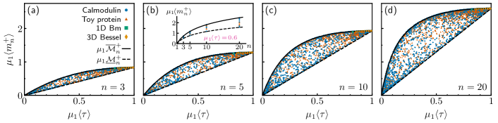
Figure S6: Expected maximal deviation from the mean, $\langle m_{n}^{+}\rangle=\langle\tau^{+}_{n}\rangle-\langle\tau\rangle$, in a sample of (a) $n=3$, (b) $n=5$, (c) $n=10$, and (d) $n=20$ independent realizations as a function of $\mu_{1}\langle\tau\rangle$. Averages are computed over $10^{7}$ draws of fixed $n$ samples and each data point corresponds to a randomly parameterized model of the calmodulin (blue) and toy protein model (red) as discussed in Sec. S5.3. Yellow points correspond to the 3D Bessel process with $a\in[0.05,0.95]$ (see Sec. S5.2) and 1D Brownian motion is shown in green. Lower bounds (dashed) and upper bounds (solid) are displayed in black, respectively. (b) The inset shows bounds and numerical data as a function of sample size $n$ for fixed $\mu_{1}\langle\tau\rangle=0.6$.

S8.3 Proof of upper bound on $\langle m_{n}^{-}\rangle$

Here, we prove the upper bound on the expected deviation of the minimum from the mean in a sample of $n$ i.i.d. realizations, i.e., an upper bound on $\langle m_{n}^{-}\rangle$. According to Eq. (S50) we have

$$\langle\tau^{-}_{n}\rangle=\int_{0}^{\infty}\mathbbm{P}(\tau^{-}_{n}\geq t)dt=\int_{0}^{\infty}S(t)^{n}dt=\int_{0}^{\infty}\left(\sum_{k}w_{k}{\rm e}^{-\mu_{k}t}\right)^{n}dt\leq\int_{0}^{\infty}\sum_{k}w_{k}{\rm e}^{-n\mu_{k}t}dt,$$ (S68)

where the last inequality follows by Jensen’s inequality since $x^{n}$ is a convex function $\forall n\geq 1,x\geq 0$. After integration of the remaining sum of exponentials we immediately find

$$\langle\tau^{-}_{n}\rangle\leq\int_{0}^{\infty}\sum_{k}w_{k}{\rm e}^{-n\mu_{k}t}dt=\sum_{k}w_{k}\frac{1}{\mu_{k}n}=\frac{\langle\tau\rangle}{n},$$ (S69)

since $\langle\tau\rangle=\sum_{k}\frac{w_{k}}{\mu_{k}}$. Consequently, we arrive at the inequality

$$\langle m_{n}^{-}\rangle=\langle\tau^{-}_{n}\rangle-\langle\tau\rangle\leq\langle\tau\rangle\left[\frac{1}{n}-1\right]\equiv\macc@depth\char 1\relax\frozen@everymath{\macc@group}\macc@set@skewchar\macc@nested@a 111{\mathcal{M}}^{-}_{n},$$ (S70)

which proves the upper bound in the second line of Eq. (14) in the Letter. Saturation occurs when $w_{k}\to 1$ for some $k$ or for degenerate systems with identical first-passage eigenvalues $\mu_{i}=\mu$, $\forall i$ for some $\mu>0$. For an illustration of the validity and sharpness of the bound for different model systems compare Fig. S7 where $\macc@depth\char 1\relax\frozen@everymath{\macc@group}\macc@set@skewchar\macc@nested@a 111{\mathcal{M}}^{-}_{n}$ is depicted as the solid black line.

S8.4 Proof of lower bound on $\langle m_{n}^{-}\rangle$

To prove the lower bound on the expected deviation of the minimum from the mean $\langle\tau^{-}_{n}\rangle$ we use an analogous reasoning as in Sec. S8.1. Recall that the ansatz (S54) (by the same argument as in Sec. S8.1) now minimizes $\langle\tau^{-}_{n}\rangle$ at fixed $\mu_{1}\langle\tau\rangle$ and gives

$$S_{\rm max}(t)^{n}=\sum_{k=1}^{n}\binom{n}{k}(1-\mu_{1}\langle\tau\rangle)^{n-k}{\rm e}^{-(n-k)t/\varepsilon}(\mu_{1}\langle\tau\rangle)^{k}{\rm e}^{-\mu_{1}kt},$$ (S71)

where we again omit, for the moment, $\lim_{\varepsilon\to 0}$ to be taken later. Consequently, we have

$$\langle\tau^{-}_{n}\rangle\geq\int_{0}^{\infty}\sum_{k=1}^{n}\binom{n}{k}(1-\mu_{1}\langle\tau\rangle)^{n-k}(\mu_{1}\langle\tau\rangle)^{k}{\rm e}^{-(\mu_{1}k+(n-k)/\varepsilon)t}dt.$$ (S72)

Again performing the integral and afterward taking the limit $\varepsilon\to 0$ (compare Eq. (S59)) yields

$$\langle\tau^{-}_{n}\rangle\geq\sum_{k=1}^{n}\binom{n}{k}(1-\mu_{1}\langle\tau\rangle)^{n-k}(\mu_{1}\langle\tau\rangle)^{k}\delta_{nk}=\frac{(\mu_{1}\langle\tau\rangle)^{n}}{\mu_{1}n},$$ (S73)

and we arrive at the inequality

$$\langle m_{n}^{-}\rangle\equiv\langle\tau^{-}_{n}\rangle-\langle\tau\rangle\geq\frac{(\mu_{1}\langle\tau\rangle)^{n}}{\mu_{1}n}-\langle\tau\rangle=\langle\tau\rangle\left[\frac{(\mu_{1}\langle\tau\rangle)^{n-1}}{n}-1\right]\equiv\underline{\mathcal{M}}_{n}^{-},$$ (S74)

which completes the proof of the announced lower bound $\underline{\mathcal{M}}_{n}^{-}$ in Eq. (14) in the Letter. We note that the bounds are saturated (i.e., the inequality becomes an equality) in systems with the above stated spectral gap (see Sec. S8.1). Finally, we remark that the upper bound $\macc@depth\char 1\relax\frozen@everymath{\macc@group}\macc@set@skewchar\macc@nested@a 111{\mathcal{M}}_{n}^{-}$ (S70) and lower bound $\underline{\mathcal{M}}_{n}^{-}$ (S74) approach the value $-\langle\tau\rangle$ from above or below, respectively, as $n\to\infty$, implying that $\lim_{n\to\infty}\langle\tau^{-}_{n}\rangle=0$, as expected. As can be seen in Fig. S7d already for $n=20$ we have $\macc@depth\char 1\relax\frozen@everymath{\macc@group}\macc@set@skewchar\macc@nested@a 111{\mathcal{M}}_{n}^{-}\to\underline{\mathcal{M}}_{n}^{-}\approx-\langle\tau\rangle$.

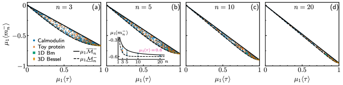
Figure S7: Expected deviation of the minimum from the mean, $\langle m_{n}^{-}\rangle=\langle\tau^{-}_{n}\rangle-\langle\tau\rangle$, in a sample of (a) $n=3$, (b) $n=5$, (c) $n=10$, and (d) $n=20$ independent realizations as a function of $\mu_{1}\langle\tau\rangle$. Averages are computed over $10^{7}$ draws of fixed $n$ samples and each data point corresponds to a randomly parameterized model of the calmodulin (blue) and toy protein model (red) as discussed in Sec. S5.3. Yellow points correspond to the 3D Bessel process with $a\in[0.05,0.95]$ (see Sec. S5.2). Lower bounds (dashed) and upper bounds (solid) are displayed in black, respectively. (b) The inset shows bounds and numerical data as a function of sample-size $n$ for fixed $\mu_{1}\langle\tau\rangle=0.6$.

References

Redner [2001]S. Redner, A Guide to First-Passage
Processes (Cambridge University Press, 2001).
Metzler et al. [2014]R. Metzler, S. Redner, and G. Oshanin, First-Passage Phenomena and their
Applications, Vol. 35 (World
Scientific, 2014).
Thorneywork et al. [2020]A. L. Thorneywork, J. Gladrow, Y. Qing,
M. Rico-Pasto, F. Ritort, H. Bayley, A. B. Kolomeisky, and U. F. Keyser, Sci. Adv. 6, 1 (2020).
Hartich and Godec [2019b]D. Hartich and A. Godec, Reaction kinetics in the few-encounter limit, in Chemical Kinetics (World
Scientific, 2019) Chap. 11, pp. 265–283.
Dougherty et al. [2002]D. B. Dougherty, I. Lyubinetsky, E. D. Williams, M. Constantin, C. Dasgupta, and S. Sarma, Phys. Rev. Lett. 89, 136102 (2002).
Constantin et al. [2003]M. Constantin, S. D. Sarma, C. Dasgupta,
O. Bondarchuk, D. B. Dougherty, and E. D. Williams, Phys. Rev. Lett. 91, 086103 (2003).
Dougherty et al. [2005]D. B. Dougherty, C. Tao,
O. Bondarchuk, W. G. Cullen, E. D. Williams, M. Constantin, C. Dasgupta, and S. D. Sarma, Phys. Rev. E 71, 021602 (2005).
Singh et al. [2019]S. Singh, P. Menczel,
D. S. Golubev, I. M. Khaymovich, J. T. Peltonen, C. Flindt, K. Saito, É. Roldán, and J. P. Pekola, Phys. Rev. Lett. 122, 230602 (2019).
Bowman et al. [2013]G. R. Bowman, V. S. Pande, and F. Noé, An Introduction to Markov State
Models and their Application to Long Timescale Molecular Simulation, Vol. 797 (Springer Science &
Business Media, 2013).
Grossfield and Zuckerman [2009]A. Grossfield and D. M. Zuckerman, Annu. Rep. Comput. Chem. 5, 23 (2009).
Grossfield et al. [2018]A. Grossfield, P. N. Patrone, D. R. Roe,
A. J. Schultz, D. W. Siderius, and D. M. Zuckerman, Living J. Comp. Mol. Sci. 1 (2018).
Note [1]Resampling methods like bootstrapping assume the data to be
representative of the inferred statistic, which is not necessarily the case
for small , possibly even when is large but finite for broad
distributions.
Prinz et al. [2011a]J.-H. Prinz, H. Wu, M. Sarich, B. Keller, M. Senne, M. Held, J. D. Chodera, C. Schütte, and F. Noé, J. Chem. Phys. 134, 174105 (2011a).
Note [5]See Supplemental Material at […] for further details,
mathematical proofs, and generalizations to arbitrary initial conditions
, as well as Refs. [49, 45, 44, 39, 43, 48].
Boucheron et al. [2013]S. Boucheron, G. Lugosi, and P. Massart, Concentration Inequalities: A
Nonasymptotic Theory of Independence (Oxford
University Press, 2013).
Note [3]Precisely, we require that satisfies the
Poincaré inequality, i.e. .
Note [4]The relaxation eigenvalue problem reads with and [154].
Noé et al. [2019]F. Noé, S. Olsson,
J. Köhler, and H. Wu, Science 365 (2019).
Braun et al. [2019]E. Braun, J. Gilmer,
H. B. Mayes, D. L. Mobley, J. I. Monroe, S. Prasad, and D. M. Zuckerman, Living J. Comp. Mol. Sci. 1, 1 (2019).
Note [6]When is discrete the integral is replaced by a sum
over states excluding the target.
Note [7] and are differentiable, convex, non-negative,
and non-decreasing functions in . The optimization is thus carried
out as where solves . The computation for follows analogously.
Note [8]Ref. [163] contains an error; the Proof of Lemma
2.3 is only valid in the regime , but the Lemma
may be shown to hold in the claimed regime [Santiago].
Note [9]However, can get arbitrary close to 0 in principle,
rendering the lower bound trivial.
Wackerly et al. [2014]D. Wackerly, W. Mendenhall, and R. L. Scheaffer, Mathematical
Statistics with Applications (Cengage Learning, 2014).
Meeker et al. [2017]W. Q. Meeker, G. J. Hahn, and L. A. Escobar, Statistical Intervals: A Guide for
Practitioners and Researchers, Vol. 541 (John Wiley & Sons, 2017).
Gardiner [2004]C. W. Gardiner, Handbook of Stochastic
Methods for Physics, Chemistry and the Natural Sciences, 3rd ed., Springer Series in Synergetics,
Vol. 13 (Springer-Verlag, Berlin, 2004).
Cowan [1998]G. Cowan, Statistical Data
Analysis (Oxford University Press, 1998).
Burden et al. [2015]R. L. Burden, J. D. Faires, and A. M. Burden, Numerical Analysis (Cengage Learning, 2015).
Supplementary Material for:

References

Gelman et al. [1995]A. Gelman, J. B. Carlin,
H. S. Stern, and D. B. Rubin, Bayesian Data Analysis (Chapman and Hall/CRC, 1995).
Brazzale et al. [2007]A. R. Brazzale, A. C. Davison, N. Reid, et al., Applied Asymptotics: Case
Studies in Small-Sample Statistics, Vol. 23 (Cambridge University Press, 2007).
Kaplan [2014]D. Kaplan, Bayesian Statistics for
the Social Sciences (Guilford Publications, 2014).
McElreath [2020]R. McElreath, Statistical
Rethinking: A Bayesian Course with Examples in R and Stan (Chapman and Hall/CRC, 2020).
Tavakoli et al. [2017]M. Tavakoli, J. N. Taylor, C.-B. Li,
T. Komatsuzaki, and S. Pressé, in Advances in Chemical Physics (John
Wiley & Sons, Inc., 2017) pp. 205–305.
Bowman et al. [2013]G. R. Bowman, V. S. Pande, and F. Noé, An Introduction to Markov State
Models and their Application to Long Timescale Molecular Simulation, Vol. 797 (Springer Science &
Business Media, 2013).
Prinz et al. [2011]J.-H. Prinz, H. Wu, M. Sarich, B. Keller, M. Senne, M. Held, J. D. Chodera, C. Schütte, and F. Noé, J. Chem. Phys. 134, 174105 (2011).
Ghosal and Van der
Vaart [2017]S. Ghosal and A. Van der
Vaart, Fundamentals of
Nonparametric Bayesian Inference, Vol. 44 (Cambridge University Press, 2017).
Gardiner [2004]C. W. Gardiner, Handbook of Stochastic
Methods for Physics, Chemistry and the Natural Sciences, 3rd ed., Springer Series in Synergetics,
Vol. 13 (Springer-Verlag, Berlin, 2004).
Stigler et al. [2011]J. Stigler, F. Ziegler,
A. Gieseke, J. C. M. Gebhardt, and M. Rief, Science 334, 512 (2011).