Verse: A Python library for reasoning about multi-agent hybrid system scenarios

Abstract

We present the Verse library with the aim of making hybrid system verification more usable for multi-agent scenarios. In Verse, decision making agents move in a map and interact with each other through sensors. The decision logic for each agent is written in a subset of Python and the continuous dynamics is given by a black-box simulator. Multiple agents can be instantiated and they can be ported to different maps for creating scenarios. Verse provides functions for simulating and verifying such scenarios using existing reachability analysis algorithms. We illustrate several capabilities and use cases of the library with heterogeneous agents, incremental verification, different sensor models, and the flexibility of plugging in different subroutines for post computations.

1 Introduction

Hybrid system verification tools have been used to analyze linear models with thousands of continuous dimensions [6, 7, 3] and nonlinear models inspired by industrial applications [7, 12]. Chen and Sankaranarayanan provide a survey of the state of the art [10]. Despite the large potential user base, current usage of this technology remains concentrated within the formal methods community. We conjecture that usability is one of the key barriers. Most hybrid verification tools [16, 29, 9, 6, 3] require the input model to be written in a tool-specific language. Tools like C2E2 [13] attempt to translate a subclass of models from the popular Simulink/Stateflow framework, but the language-barrier goes deeper than syntax. The verification algorithms are based on variants of the hybrid automaton [4, 20, 23] which require the discrete states (or modes) to be spelled out explicitly as a graph, with guards and resets labeling the edges.

In contrast, the code for simulating a multi-agent scenario would be written in an expressive programming language. Each agent will have a decision logic and some continuous dynamics. A complex scenario would be composed by putting together a collection of agents; it may use a map which brings additional structure and constraints to the agent’s decisions and interactions. Describing or translating such scenarios for hybrid verification is a far cry from the capabilities of current tools.

In this paper, we present Verse , a Python library that aims to make hybrid technologies more usable for multi-agent scenarios. An agent’s decision logic is written in an expressive subset of Python (See Fig. 2). This program can access the relevant features of the map and parts of the states of the other agents. The continuous dynamics of an agent has to be supplied as a black-box simulation function. Multiple agents with different dynamics and different decision logics are instantiated to create a Verse scenario.

Verse provides functions for performing systematic simulation and verification of such scenarios through reachability analysis. An agent’s decision logic can allow nondeterministic choices. If multiple Python if conditions are satisfied at a given state, then both branches are explored. For example, Fig. 1(center) shows simulations in which the red drone on track T1 nears the blue and nondeterministically switches to tracks T0 and T2. Similarly, the verify function propagates uncertainty in the initial states through branches. Safety requirements written with assert can be checked via reachability analysis. While the functions for traversal and ${post}$ computation are based on known algorithms, new ones can be implemented and the library vastly simplifies specification of hybrid multi-agent scenarios.

The key concept that makes the above functionalities tractable and specifications expressive is the map abstraction. A Verse map defines a set of tracks that agents can follow. While a map may have infinitely many tracks, they fall in a finite number of track modes. For example, in Fig. 1 each layer in the map is assigned to a track mode (T0-2) and the tracks between each pair of layers are also assigned to a track mode (M10, M01 etc.). Further, when an agent makes a decision and changes its internal mode (called tactical mode, which is different from the track mode), for example from Normal to MoveUp, the map object determines the new track mode for the agent. For an agent on track T1, its new track mode will be M10. This map abstraction allows portability of an agent’s decision logic across different maps as long as they have the same interface or track modes. It makes Verse suited for multi-agent scenarios, arising in motion control [19], air-traffic management [14], and the study of tactical collision avoidance [26].

In summary, the main contributions of this paper are: (1) an expressive framework for specifying and simulating multi-agent hybrid scenarios on interesting maps (Section 3), (2) a library of powerful functions for building verification algorithms based on reachability analysis (Section 5), and (3) illustrations of several capabilities and use cases of the library with heterogeneous agents, incremental verification, different sensor models, and the flexibility of plugging in different subroutines for post computations (Section 6).

Related work.

There are a number of powerful tools for creating, simulating, and testing complex multi-agent scenarios [17, 34, 8, 27]. For instance, Scenic [17] uses a probabilistic programming language for guided sampling, simulations, and falsification, Flow [34] integrates the SUMO [25] traffic simulator for reinforcement learning, AAM-GYM [8] can generate and simulate scenarios for testing AI algorithms in advanced air mobility, and GRAIC [27] has been used for testing racing controllers in dynamic environments. While the models created in these tools can be very flexible and expressive, they are not readily amenable to formal verification.

Interactive theorem provers have been used for modeling and verification of multi-agent, distributed and hybrid systems [15, 18, 24, 35]. Most notably KeYmeraX [18] uses quantified differential dynamic logic for specifying multi-agent scenarios and supports speculative proof search and user defined tactics. Isabelle/HOL [15], PVS [24], and Maude [35] have also been used for limited classes of hybrid systems. These approaches require significant levels of user expertise to interact with.

This work is closest to the tool presented in [31], which also supports multiple agents and reachability analysis. However, Verse significantly improves usability by allowing (a) Python for the decision logics and (b) complex maps. The theoretical ideas of Sibai et al. [30, 31], in exploiting symmetries and caching are complementary to our contributions and could indeed be incorporated to improve the verification algorithms in Verse.

2 Overview of Verse

We will highlight the key features of Verse with an example. Consider two drones flying along three parallel figure-eight tracks that are vertically separated in space (shown by black lines in Fig. 1). Each drone has a simple collision avoidance logic: if it gets too close to another drone on the same track, then it switches to either the track above or the one below. A drone on T1 has both choices. Verse enables creation, simulation, and verification of such scenarios using Python, and provides a collection of powerful functions for building new analysis algorithms for such scenarios.

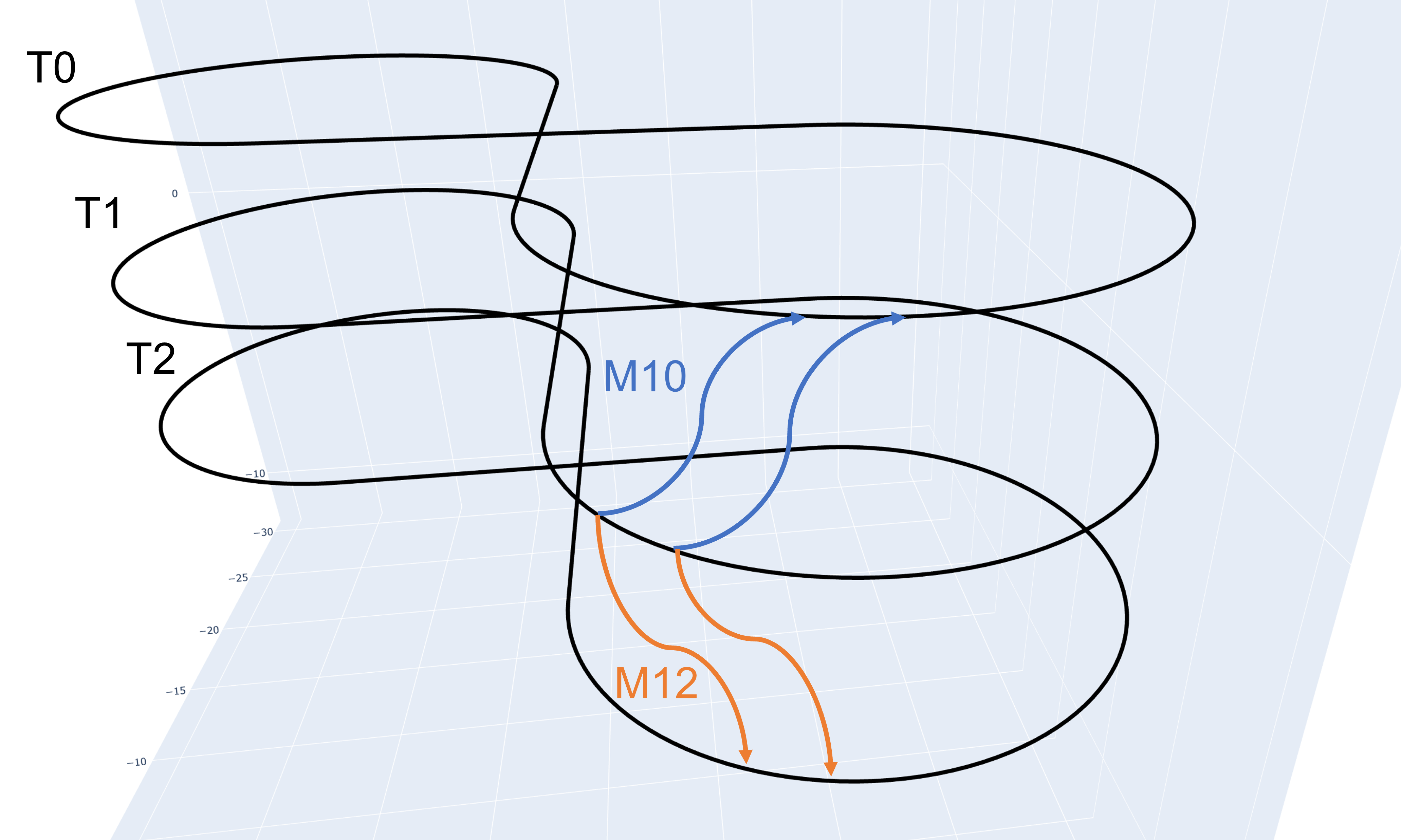
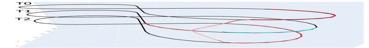
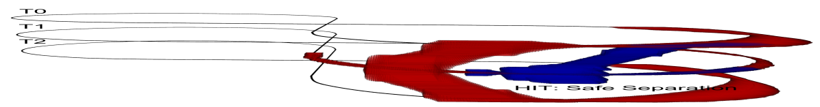
Figure 1: Left: A 3-d figure-8 map with example track mode labels. Center: Simulation of a red drone nearing the blue drone on T1 and nondeterministically moving to T0 or T2. Both branches are computed by Verse’s simulate function. Right: Computed reachable sets of the two drones cover more possibilities: both drones are allowed to switch tracks when they get close. All four branches are explored by Verse and one is found to violate safety.

Creating scenarios.

Agents like the drones in this example are described by a simulator and a decision logic. The decision logic has to be written in an expressive subset of Python (see code in Fig. 2 and Appendix 0.B for more details). The decision logic for an ego agent takes as input its current state and the (observable) states of the other agents, and updates the discrete state or the mode of the ego agent. It may also update the continuous state of the ego agent. The mode of an agent, as we shall see later in Section 3.2, has two parts—a tactical mode corresponding to agent’s decision or discrete state, and a track mode that is determined by the map. Using the any and all functions, the agent’s decision logic can quantify over other agents in the scene. For example, in lines 41-43 of Fig. 2 an agent updates its tactical mode to begin a track change if there is any agent near it.

Verse will parse this decision logic to internally construct the transition graph of the hybrid model with guards and resets. The simulator can be written in any language and is treated as a black-box. For the examples discussed in this paper, the simulators are also written in Python. Safety requirements can be specified using assert statements (see Fig. 5).

⬇

from enum import Enum, auto

import copy

class TacticalMode(Enum):

Normal = auto()

MoveUp = auto()

MoveDown = auto()

class TrackMode(Enum):

T0 = auto()

T1 = auto()

T2 = auto()

M01 = auto()

M10 = auto()

M12 = auto()

M21 = auto()

class State:

x:float

y:float

z:float

vx:float

vy:float

vz:float

tactical_mode: TacticalMode

track_mode: TrackMode

def __init__(self, x, y, z, vx, vy, vz, tactical_mode, track_mode):

pass

def is_close(ego, other):

res = ego.x-other.x>-5 and ego.x-other.x<5 and \

ego.x-other.x<-4 and ego.x-other.x>4 and \

ego.y-other.y>-5 and ego.y-other.y<5 and \

ego.y-other.y<-4 and ego.y-other.y>4

return res

def decisionLogic(ego: State, others: List[State], track_map):

next = copy.deepcopy(ego)

if ego.tactical_mode == TacticalMode.Normal:

if any((is_close(ego, other) and ego.track_mode==other.track_mode) for other in others):

next.tactical_mode = TacticalMode.MoveDown

next.track_mode = track_map.h(ego.track_mode, ego.tactical_mode, TacticalMode.MoveDown)

if any((is_close(ego, other) and ego.track_mode==other.track_mode) for other in others):

next.tactical_mode = TacticalMode.MoveUp

# …

if ego.tactical_mode == TacticalMode.MoveUp:

if in_interval(track_map.altitude(ego.track_mode)-ego.z, -1, 1):

next.tactical_mode = TacticalMode.Normal

next.track_mode = track_map.h(ego.track_mode, ego.tactical_mode, TacticalMode.Normal)

# …

return next

if ego.tactical_mode == TacticalMode.MoveUp:

if track_map.altitude(ego.track_mode)-ego.z>-1 and track_map.altitude(ego.track_mode)-ego.z<1:

next.tactical_mode = TacticalMode.Normal

next.track_mode = track_map.h(ego.track_mode, ego.tactical_mode, TacticalMode.Normal)

if ego.tactical_mode == TacticalMode.MoveDown:

if track_map.altitude(ego.track_mode)-ego.z>-1 and track_map.altitude(ego.track_mode)-ego.z<1:

next.tactical_mode = TacticalMode.Normal

next.track_mode = track_map.h(ego.track_mode, ego.tactical_mode, TacticalMode.Normal)

return next

Figure 2: Decision Logic Code Snippet from drone$\_$controller.py.

Maps and sensors.

The map of a scenario specifies the tracks that the agents can follow. Besides creating from scratch, Verse provides functions that automatically generates map objects from OpenDRIVE [5] files. The sensor function defines which variables from an agent are visible to other agents. The default sensor function allows all agents to see all variables; we discuss how the sensor function can be modified to include bounded noise in Section 6.1. A map, a sensor and a collection of (compatible) agents together define a scenario object (Fig. 3). In the first few lines the drone agents are created, initialized, and added to the scenario object. A scenario can have heterogeneous agents with different decision logics.

⬇

from audioop import tomono

from quadrotor_agent import QuadrotorAgent

from verse import Scenario

# from verse.plotter.plotter2D import *

from verse.plotter.plotter3D_new import *

from verse.map.example_map.simple_map_3d import SimpleMap1, SimpleMap2, SimpleMap3, SimpleMap4

from verse.sensor.example_sensor.quadrotor_sensor import QuadrotorSensor

import os

import json

import plotly.graph_objects as go

from enum import Enum, auto

from gen_json import write_json, read_json

import pyvista as pv

from verse.plotter.plotter3D import *

class CraftMode(Enum):

Normal = auto()

Switch_Down = auto()

Switch_Up = auto()

Switch_Left = auto()

Switch_Right = auto()

class LaneMode(Enum):

Lane0 = auto()

Lane1 = auto()

Lane2 = auto()

if __name__ == "__main__":

scenario = Scenario()

drone_red = DroneAgent(’drone_red’, file_name=’drone_controller.py’)

drone_red.set_initial([init_l_1, init_u_1],(CraftMode.Normal, TrackMode.T1))

scenario.add_agent(drone_red)

drone_blue = DroneAgent(’drone_blue’, file_name=’drone_controller.py’)

scenario.add_agent(drone_blue)

# …

scenario.set_map(M6())

scenario.set_sensor(BaseSensor())

# …

#traces = scenario.simulate(40, time_step)

traces = scenario.verify(40, time_step)

fig = pv.Plotter()

fig = plot3dReachtube(traces, ’Agent1’, 1, 2, 3, ax = fig, color = ’r’)

fig = plot3dReachtube(traces, ’Agent2’, 1, 2, 3, ax = fig, color = ’b’)

# …

fig.show()

Figure 3: Scenario Specification File Snippet

Simulation and reachability.

Once a scenario is defined, Verse’s simulate function can generate simulation(s) of the system, which can be stored and plotted. As shown earlier in Fig. 1, a simulation from a single initial state explores all possible branches that can be generated by the decision logics of the interacting agents, upto a specified time horizon. Verse can verify the safety assertions of a scenario with the verify function. It computes the over-approximations of the reachable sets for each agent, and checks these against the predicates defined by the assertions. Fig. 1 visualizes the result of such a computation performed using the verify function. In this example, the safety condition is violated when the blue drone moves downward to avoid the red drone. The other branches of the scenario are proved to be safe. The simulate and verify functions save a copy of the resulting execution tree, which can be loaded and traversed to analyze the sequences modes and states that leads to safety violations.

Building advanced functions.

Verse library provides powerful functions to implement advanced verification algorithms. Section 5.2 explains how users can modify the basic reachability algorithm to save computing time in repeated verification of similar scenarios using caching and incremental verification. Verse also makes it convenient to plug in different reachability subroutines. The experiments in Section 6.1 show how the sensor can be useful when modeling realistic inputs to the controllers and Section 6.3 describes verification when dynamics have uncertainty.

3 Scenarios in Verse

A scenario in Verse is specified by a map, a collection of agents in that map, and a sensor function that defines the part of each agent that is visible to other agents. We describe these components below and in Section 4 we will discuss how they formally define a hybrid system.

3.1 Tracks, modes, and maps

A workspace ${W}$ is an Euclidean space in which the agents reside (For example, a compact subset of ${\mathbb{R}}^{2}$ or ${\mathbb{R}}^{3}$). An agent’s continuous dynamics makes it roughly follow certain continuous curves in ${W}$, called tracks, and occasionally the agent’s decision logic changes the track. Formally, a track is simply a continuous function ${\omega}:[0,1]\rightarrow{W}$, but not all such functions are valid tracks. A map $\mathcal{M}$ defines the set of tracks ${\Omega}_{\mathcal{M}}$ it permits. In a highway map, some tracks will be aligned along the lanes while others will correspond to merges and exits.

We assume that an agent’s decision logic does not depend on exactly which of the infinitely many tracks it is following, but instead, it depends only on which type of track it is following or the track mode. In the example in Section 2, the track modes are T0, T1, M01, etc. Every (blue) track for transitioning from point on T0 to the corresponding point on T1 has track mode M01. A map has a finite set of track modes ${L}_{\mathcal{M}}$, a labeling function ${V}_{\mathcal{M}}:{\Omega}_{\mathcal{M}}\rightarrow{L}_{\mathcal{M}}$ that gives the track mode for a track. It also has a mapping ${g}_{\mathcal{M}}:{W}\times{L}_{\mathcal{M}}\rightarrow{\Omega}_{\mathcal{M}}$ that gives a specific track from a track mode and a specific position in the workspace.

Finally, a Verse agent’s decision logic can change its internal mode or tactical mode (E.g., Normal to MoveUp). When an agent changes its tactical mode, it may also update the track it is following and this is encoded in another function: ${h}_{\mathcal{M}}:{L}_{\mathcal{M}}\times{P}\times{P}\rightarrow{L}_{\mathcal{M}}$ which takes the current track mode, the current and the next tactical mode, and generates the new track mode the agent should follow. For example, when the tactical mode of a drone changes from Normal to MoveUP while it is on T1, this map function ${h}_{\mathcal{M}}(\texttt{T1},\texttt{Normal},\texttt{MoveUp})=\texttt{M10}$ informs that the agent should follow a track with mode M10. These sets and functions together define a Verse map object $\mathcal{M}=\langle{L}_{\mathcal{M}},{V}_{\mathcal{M}},{g}_{\mathcal{M}},{h}_{\mathcal{M}}\rangle$. We will drop the subscript $\mathcal{M}$, when the map being used is clear from context.

3.2 Agents

A Verse agent is defined by modes and continuous state variables, a decision logic that defines (possibly nondeterministic) discrete transitions, and a flow function that defines continuous evolution. An agent $\mathcal{A}$ is compatible with a map $\mathcal{M}$ if the agent’s tactical modes ${P}$ are a subset of the allowed input tactical modes for ${h}$. This makes it possible to instantiate the same agent on different compatible maps. The mode space for an agent instantiated on map $\mathcal{M}$ is the set ${D}={L}\times{P}$, where ${L}$ is the set of track modes in $\mathcal{M}$ and ${P}$ is the set of tactical modes of the agent. The continuous state space is ${X}={W}\times{Z}$, where ${W}$ is the workspace (of $\mathcal{M}$) and ${Z}$ is the space of other continuous state variables. The (full) state space is the Cartesian product ${Y}={X}\times{D}$. In the two-drone example in Section 2, the continuous states variables $px,py,pz,vx,vy,vz$ are the positions and velocities along the three axes of the workspace. The modes are $\langle\texttt{Normal},\texttt{T1}\rangle$, $\langle\texttt{MoveUp},\texttt{M10}\rangle$, etc.

An agent $\mathcal{A}$ in map $\mathcal{M}$ with $k-1$ other agents is defined by a tuple $\mathcal{A}=\langle{Y},{Y}^{0},{G},{R},{F}\rangle$, where ${Y}$ is the state space, ${Y}^{0}\subseteq{Y}$ is the set of initial states. The guard ${G}$ and reset ${R}$ functions jointly define the discrete transitions. For a pair of modes ${d},{d}^{\prime}\in{D},$ ${G}({d},{d}^{\prime})\subseteq{X}^{k}$ defines the condition under which a transition from ${d}$ to ${d}^{\prime}$ is enabled. The ${R}({d},{d}^{\prime}):{X}^{k}\rightarrow{X}$ function specifies how the continuous states of the agent are updated when the mode switch happens. Both of these functions take as input the sensed continuous states of all the other $k-1$ agents in the scenario. Details about the sensor which transmits state information across agents is discussed in Section 3.3. The ${G}$ and the ${R}$ functions are actually not defined separately, but are extracted by the Verse parser from a block of structured Python code as shown in Fig. 2. The discrete states in the if condition and the assignments define the source and destination of discrete transition. The if conditions involving continuous states define the guard for the transitions and the assignments of continuous states define the reset. Expressions with any and all functions are unrolled to disjunctions and conjunctions according to the number of agents $k$.

For example, Lines 47-50 define transitions $\langle\texttt{MoveUp},\texttt{M10}\rangle$ to $\langle\texttt{Normal},\texttt{T0}\rangle$ and $\langle\texttt{MoveUp},\texttt{M21}\rangle$ to $\langle\texttt{Normal},\texttt{T1}\rangle$. The change of track mode is given by the ${h}$ function. The guard for this transition comes from the if condition at Line 48. For example, ${G}(\langle\texttt{MoveUp},\texttt{M10}\rangle,\langle\texttt{Normal},\texttt{T0}\rangle)=\{{x}\mid-1<\texttt{T0}.pz-{x}.pz<1\}$ for ${x}\in{X}$. Here continuous states remain unchanged after transition.

The final component of the agent is the flow function ${F}:{X}\times{D}\times{\mathbb{R}}^{\geq 0}\rightarrow{X}$ which defines the continuous time evolution of the continuous state. For any initial condition $\langle{x}^{0},{d}^{0}\rangle\in Y$, $F({x}^{0},{d}^{0})(\cdot)$ gives the continuous state of the agent as a function of time. In this paper, we use $F$ as a black-box function (see footnote 2).

3.3 Sensors and scenarios

For a scenario with $k$ agents, a sensor function $\mathcal{S}:{Y}^{k}\rightarrow{Y}^{k}$ defines the continuous observables as a function of the continuous state. For simplifying exposition, in this paper we assume that observables have the same type as the continuous state $Y$, and that each agent $i$ is observed by all other agents identically. This simple, overtly transparent sensor model, still allows us to write realistic agents that only use information about nearby agents. In a highway scenario, the observable part of agent $j$ to another agent $i$ may be the relative distance $y_{j}=x_{j}-x_{i}$, and vice versa, which can be computed as a function of the continuous state variables $x_{j}$ and $x_{i}$. A different sensor function which gives nondeterministic noisy observations, appears in Section 6.1.

A Verse scenario ${SC}$ is defined by (a) a map $\mathcal{M}$, (b) a collection of $k$ agent instances $\{\mathcal{A}_{1}...\mathcal{A}_{k}\}$ that are compatible with $\mathcal{M}$, and (c) a sensor $\mathcal{S}$ for the $k$ agents. Since all the agents are instantiated on the same compatible map $\mathcal{M}$, they share the same workspace. Currently, we require agents to have identical state spaces, i.e., ${Y}_{i}={Y}_{j}$, but they can have different decision logics and different continuous dynamics.

4 Verse scenario to hybrid verification

In this section, we define the underlying hybrid system ${H}({SC})$, that a Verse scenario ${SC}$ specifies. The verification questions that Verse is equipped to answer are stated in terms of the behaviors or executions of ${H}({SC})$. Verse’s notion of a hybrid automaton is close to that in Definition 5 of [12]. As usual, the automaton has discrete and continuous states and discrete transitions defined by guards and resets. The only uncommon aspect in [12] is that the continuous flows may be defined by a black-box simulator functions, instead of white-box analytical models (see footnote 2).

Given a scenario with $k$ agents ${SC}=\langle\mathcal{M},\{\mathcal{A}_{1},...\mathcal{A}_{k}\},\mathcal{S},{P}\rangle$, the corresponding hybrid automaton ${H}({SC})=\langle\textbf{X},\textbf{X}^{0},\textbf{D},\textbf{D}^{0},\textbf{G},\textbf{R},\textbf{TL}\rangle$, where

1. $\textbf{X}:=\prod_{i}{X}_{i}$ is the continuous state space. An element $\textbf{x}\in\textbf{X}$ is called a state. $\textbf{X}^{0}:=\prod_{i}{X}_{i}^{0}\subseteq\textbf{X}$ is the set of initial continuous states.

2. $\textbf{D}:=\prod_{i}{D}_{i}$ is the mode space. An element $\textbf{d}\in\textbf{D}$ is called a mode. $\textbf{D}^{0}:=\prod_{i}{D}_{i}^{0}\subseteq\textbf{D}$ is the finite set of initial modes.

3. For a mode pair $\textbf{d},\textbf{d}^{\prime}\in\textbf{D}$, $\textbf{G}(\textbf{d},\textbf{d}^{\prime})\subseteq\textbf{X}$ defines the continuous states from which a transition from d to $\textbf{d}^{\prime}$ is enabled. A state $\textbf{x}\in\textbf{G}(\textbf{d},\textbf{d}^{\prime})$ iff there exists an agent $i\in\{1,...,k\}$, such that $\textbf{x}_{i}\in{G}_{i}(\textbf{d}_{i},\textbf{d}_{i}^{\prime})$ and $\textbf{d}_{j}=\textbf{d}_{j}^{\prime}$ for $j\neq i$.

4. For a mode pair $\textbf{d},\textbf{d}^{\prime}\in\textbf{D}$, $\textbf{R}(\textbf{d},\textbf{d}^{\prime}):\textbf{X}\rightarrow\textbf{X}$ defines the change of continuous states after a transition from d to $\textbf{d}^{\prime}$. For a continuous state $\textbf{x}\in\textbf{X}$, $\textbf{R}(\textbf{d},\textbf{d}^{\prime})(\textbf{x})={R}_{i}(\textbf{d}_{i},\textbf{d}_{i}^{\prime})(\textbf{x})\text{ if }\textbf{x}\in{G}_{i}(\textbf{d}_{i},\textbf{d}_{i}^{\prime})$, otherwise $=\textbf{x}_{i}$.

5. TL is a set of pairs $\langle\xi,\textbf{d}\rangle$, where the trajectory $\xi:[0,T]\rightarrow\textbf{X}$ describes the evolution of continuous states in mode $\textbf{d}\in\textbf{D}$. Given $\textbf{d}\in\textbf{D},\textbf{x}^{0}\in\textbf{X}$, $\xi$ should satisfy $\forall t\in{\mathbb{R}}^{\geq 0},\xi_{i}(t)=F_{i}(\textbf{x}^{0}_{i},\textbf{d}_{i})(t)$.

Proposition 1

If a scenario with $k$ agents ${SC}=\langle\mathcal{M},\{\mathcal{A}_{1},...,\mathcal{A}_{k}\},\mathcal{S},{P}\rangle$, satisfies the following: (1) map and the agents are compatible, (2) all agents have identical sets of states and modes, ${Y}_{i}={Y}_{j}$, and (3) agent states match the input type of $\mathcal{S}$, then ${H}({SC})$ is a valid hybrid system.

We denote by $\xi.fstate$, $\xi.lstate$, and $\xi.ltime$ the initial state $\xi(0)$, the last state $\xi(T)$, and $\xi.ltime=T$. For a sampling parameter $\delta>0$ and a length $m$, a $\delta$-execution of a hybrid automaton ${H}={H}({SC})$ is a sequence of $m$ labeled trajectories ${\alpha}:=\langle\xi^{0},\textbf{d}^{0}\rangle,...,\langle\xi^{m-1},\textbf{d}^{m-1}\rangle$, such that (1) $\xi^{0}.fstate\in\textbf{X}^{0},\textbf{d}^{0}\in\textbf{D}^{0}$, (2) For each $i\in\{1,...,m-1\}$, $\xi_{i}.lstate\in\textbf{G}(\textbf{d}^{i},\textbf{d}^{i+1})$ and $\xi^{i+1}.fstate=\textbf{R}(\textbf{d}^{i},\textbf{d}^{i+1})(\xi^{i}.lstate)$, and (3) For each $i\in\{1,...,m-1\}$, $\xi^{i}.ltime=\delta$ for $i\neq m-1$ and $\xi^{i}.ltime\leq\delta$ for $i=m-1$.

We define the first and last state of an execution ${\alpha}=\langle\xi^{0},\textbf{d}^{0}\rangle,...,\langle\xi^{m-1},\textbf{d}^{m-1}\rangle$ as ${\alpha}.fstate=\xi^{0}.fstate$, ${\alpha}.lstate=\xi^{m-1}.lstate$ and the first and last mode as ${\alpha}.fmode=\textbf{d}^{0}$ and ${\alpha}.lmode=\textbf{d}^{m-1}$. The set of reachable states is defined by ${Reach_{{H}}}:=\{{\alpha}.lstate\mid{\alpha}\text{ is an execution of }{H}\}$. In addition, we denote the reachable states in a specific mode $\textbf{d}\in\textbf{V}$ as ${Reach_{{H}}}(\textbf{d})$ and ${Reach_{{H}}}(T)$ to be the set of reachable states at time $T$. Similarly, denoting the unsafe states for mode d as $\textbf{U}(\textbf{d})$, the safety verification problem for ${H}$ can be solved by checking whether $\forall\textbf{d}\in\textbf{D}$, ${Reach_{{H}}}(\textbf{d})\cap\textbf{U}(\textbf{d})=\emptyset$. Next, we discuss Verse functions for verification via reachability.

5 Building verification algorithms in Verse

The Verse library comes with several built-in verification algorithms, and it provides functions that users can be use to implement powerful new algorithms. We first describe the basic building blocks and in Sections 5.2 and 6.2 we discuss more advanced use cases and algorithms.

5.1 Reachability analysis

Consider a scenario ${SC}$ with $k$ agents and the corresponding hybrid automaton ${H}({SC})$. For a pair of modes, $\textbf{d},\textbf{d}^{\prime}$ the standard discrete ${post}_{\textbf{d},\textbf{d}^{\prime}}:\textbf{X}\rightarrow\textbf{X}$ and continuous ${post}_{\textbf{d},\delta}:\textbf{X}\rightarrow\textbf{X}$ operators are defined as follows: For any state $\textbf{x},\textbf{x}^{\prime}\in\textbf{X}$, ${post}_{\textbf{d},\textbf{d}^{\prime}}(\textbf{x})=\textbf{x}^{\prime}$ iff $\textbf{x}\in\textbf{G}(\textbf{d},\textbf{d}^{\prime})$ and $\textbf{x}^{\prime}=\textbf{R}(\textbf{d},\textbf{d}^{\prime})(\textbf{x})$; and, ${post}_{\textbf{d},\delta}(\textbf{x})=\textbf{x}^{\prime}$ iff $\forall i\in{1,...,k}$, $\textbf{x}_{i}^{\prime}={F}_{i}(\textbf{x}_{i},\textbf{d}_{i},\delta)$. These operators are also lifted to sets of states in the usual way. Verse provides postCont to compute ${post}_{\textbf{d},\delta}$ and postDisc to compute ${post}_{\textbf{d},\textbf{d}^{\prime}}$. Instead of computing the exact post, postCont and postDisc compute over-approximations using improved implementations of the algorithms in [12]. Verse’s verify function implements a reachability analysis algorithm using these post operators (Algorithm 1). This algorithm constructs an execution tree ${Tree}=\langle{V},{E}\rangle$ up to depth $m$ in breadth first order. Each vertex $\langle\textbf{S},\textbf{d}\rangle\in{V}$ is a pair of a set of states and a mode. The root is $\langle\textbf{X}^{0},\textbf{d}^{0}\rangle$. There is an edge from $\langle\textbf{S},\textbf{d}\rangle$ to $\langle\textbf{S}^{\prime},\textbf{d}^{\prime}\rangle$, iff $\textbf{S}^{\prime}={post}_{\textbf{d}^{\prime},\delta}({post}_{\textbf{d},\textbf{d}^{\prime}}(\textbf{S}))$.

Algorithm 1

1:function verify($\langle\textbf{X}^{0},\textbf{d}^{0}\rangle,{H},{m},\delta$)

2:   $root\leftarrow\langle\textbf{X}^{0},\textbf{d}^{0}\rangle$

3:   $depth\leftarrow 0$

4:   $queue\leftarrow[\langle\langle\textbf{X}^{0},\textbf{d}^{0}\rangle,depth\rangle]$

5:   while $queue\neq\emptyset$ and $depth\leq{m}$ do

6:      $\langle{\langle\textbf{S},\textbf{d}\rangle},depth\rangle\leftarrow queue.\texttt{dequeue}()$

7:      for $\textbf{d}^{\prime}$, s.t. $\textbf{G}(\textbf{d},\textbf{d}^{\prime})$ do

8:         if $\textbf{S}\cap\textbf{G}(\textbf{d},\textbf{d}^{\prime})\neq\emptyset$ then

9:            ${\langle\textbf{S}^{\prime},\textbf{d}^{\prime}\rangle}\leftarrow\langle\texttt{postCont}(\texttt{postDisc}(\textbf{S},\textbf{d},\textbf{d}^{\prime}),\textbf{d}^{\prime},\delta),\textbf{d}^{\prime}\rangle$;

10:            ${\langle\textbf{S},\textbf{d}\rangle}.\texttt{addChild}(\langle\textbf{S}^{\prime},\textbf{d}^{\prime}\rangle)$

11:            $queue.\texttt{add}(\langle{\langle\textbf{S}^{\prime},\textbf{d}^{\prime}\rangle},depth+1\rangle)$                   

12:   return $root$

Proposition 2

For hybrid automaton ${H}={H}({SC})$, let ${Tree}=\langle{V},{E}\rangle$ be the execution tree with depth $T$ constructed by verify, then for each level $t\in\{0,...,T\}$, ${Reach_{{H}}}(\delta t)=V(t)$, where ${V}(t)$ is the union of the states in the vertices at depth $t$.

Proposition 2 holds when the post computations are exact. However, typically, we rely on techniques that compute the over-approximations of the actual post, in which, ${V}(t)$ over-approximates ${Reach_{{H}}}(\delta t)$. Currently, Verse implements only bounded time reachability, however, basic unbounded time analysis with fixed-point checks could be added following [12, 30].

5.2 Incremental Verification

During the design-analysis process, users perform many simulation and verification runs on slightly tweaked scenarios. Can we do better than starting each verification run from scratch? In Verse, we have implemented an incremental analysis algorithm that improves the performance of simulate and verify by reusing data from previous verification runs. This algorithm also illustrates how Verse can be used to implement different algorithms.

Consider two hybrid automata ${H}_{i}={H}({SC}_{i}),$ $i\in\{1,2\}$ that only differ in the discrete transitions. That is, (1) $\textbf{X}_{2}=\textbf{X}_{1}$, (2) $\textbf{D}_{2}=\textbf{D}_{1}$, and (3) $\textbf{TL}_{2}=\textbf{TL}_{1}$, while the initial conditions, the guards, and the resets are slightly different. ${SC}_{1}$ and ${SC}_{2}$ have the same sensors, maps, and agent flow functions. Let ${Tree}_{1}=\langle{V}_{1},{E}_{1}\rangle$ and ${Tree}_{2}=\langle{V}_{2},{E}_{2}\rangle$ be the execution trees for ${H}_{1}$ and ${H}_{2}$. Our idea of incremental verification is to reuse some of the computations in constructing the tree for ${H}_{1}$ in computing the same for ${H}_{2}$.

Recall that in verify, expanding each vertex $\langle\textbf{S}_{1},\textbf{d}_{1}\rangle$ of ${Tree}_{1}$ with a possible mode involves a guard check, a computation of ${post}_{\textbf{d},\textbf{d}^{\prime}}$, and ${post}_{\textbf{d},\delta}$. The verifyInc algorithm avoids performing these computations while constructing ${Tree}_{2}$ by reusing those computations from ${Tree}_{1}$, if possible. To this end, verifyInc is endowed with two caches: ${C_{g}}$ stores information about discrete transitions and ${C_{f}}$ stores information about continuous flows. The key to ${C_{g}}$ is a vertex $\langle\textbf{S}_{2},\textbf{d}_{2}\rangle\in{V}_{2}$, a guard $\textbf{G}_{2}(\textbf{d}_{2},\textbf{d}_{2}^{\prime})$ and a reset $\textbf{R}_{2}(\textbf{d}_{2},\textbf{d}_{2}^{\prime})$ for a mode pair. The retrieved data from ${C_{g}}$ will be a pair $\langle s,v^{\prime}\rangle$ where $s\in\{{\texttt{sat}},{\texttt{unsat}},{\texttt{unknown}}\}$ is the guard checking result for $\textbf{S}_{2}$ and $\textbf{G}_{2}(\textbf{d},\textbf{d}^{\prime})$ and $v^{\prime}=\langle{post}_{\textbf{d},\textbf{d}^{\prime}}(\textbf{S}_{2}),\textbf{d}^{\prime}\rangle$ is the vertex after applying post. A cache hit can happen if there exists an entry in the cache with key match exactly with $\langle\langle\textbf{S}_{2},\textbf{d}_{2}\rangle,\textbf{G}_{2}(\textbf{d}_{2},\textbf{d}_{2}^{\prime}),\textbf{R}_{2}(\textbf{d}_{2},\textbf{d}_{2}^{\prime})\rangle$. If $\langle{\langle\textbf{S}_{2},\textbf{d}_{2}\rangle},\textbf{G}_{2}(\textbf{d}_{2},\textbf{d}_{2}^{\prime}),\textbf{R}_{2}(\textbf{d}_{2},\textbf{d}_{2}^{\prime})\rangle\in{C_{g}}$ and $s={\texttt{sat}}$, then we know from ${C_{g}}$ that $\textbf{S}_{2}$ satisfies $\textbf{G}_{2}(\textbf{d}_{2},\textbf{d}_{2}^{\prime})$ and the post of S can be retrieved from the cache $v^{\prime}=\langle{post}_{\textbf{d},\textbf{d}^{\prime}}(\textbf{S}_{2}),\textbf{d}_{2}^{\prime}\rangle$. If $\langle{\langle\textbf{S}_{2},\textbf{d}_{2}\rangle},\textbf{G}_{2}(\textbf{d}_{2},\textbf{d}_{2}^{\prime}),\textbf{R}_{2}(\textbf{d}_{2},\textbf{d}_{2}^{\prime})\rangle\in{C_{g}}$ but $s={\texttt{unsat}}$, then $\textbf{S}_{2}$ does not satisfy the guard $\textbf{G}_{2}(\textbf{d}_{2},\textbf{d}_{2}^{\prime})$ and $v^{\prime}=\texttt{none}$. If $\langle{\langle\textbf{S}_{2},\textbf{d}_{2}\rangle},\textbf{G}_{2}(\textbf{d}_{2},\textbf{d}_{2}^{\prime}),\textbf{R}_{2}(\textbf{d}_{2},\textbf{d}_{2}^{\prime})\rangle\notin{C_{g}}$, then $s={\texttt{unknown}}$, $v^{\prime}=\texttt{none}$ and the guard checking and post computation from $\textbf{S}_{2}$ will need to happen afresh for ${H}_{2}$.

The second cache constructed is ${C_{f}}$. The key to the cache will be a vertex $\langle\textbf{S},\textbf{d}\rangle$. A cache hit can happen if there exist an entry in the cache $\langle\textbf{S}^{\prime},\textbf{d}^{\prime}\rangle$ such that $\textbf{S}\subseteq\textbf{S}^{\prime}$ and $\textbf{d}=\textbf{d}^{\prime}$ and the retrieved value from the cache will be $\textbf{S}^{\prime\prime}={post}_{\textbf{d},\delta}(\textbf{S}^{\prime})\supseteq{post}_{\textbf{d},\delta}(\textbf{S})$.

Similar to verify, for each vertex in the tree, verifyInc expands all possible mode transitions (Line 10).The full algorithm is shown in Algorithm 2 for completeness and we skip the detailed description owing to space limitations. verifyInc checks ${C_{g}}$ or ${C_{f}}$ before every ${post}$ computation to retrieve and reuse computations when possible. The caches can save information from any number of previous executions, so verifyInc can be even more efficient than verify when running many consecutive verification runs.

Proposition 3

Given the caches ${C_{g}}$ and ${C_{f}}$ constructed while constructing ${Tree}_{1}$ for ${H}_{1}$, the tree ${Tree}_{2}$ constructed by verifyInc is sound. That is

$${Reach_{{H}_{2}}}(\delta t)\subseteq{V}_{2}(t),\forall t\in\{0,...,T\}$$

Proof

The proof relies on verifyInc’s design ensuring that the cache data is always an over approximation of the actual post computations. Consider ${C_{g}}$ and ${C_{f}}$ constructed while constructing ${Tree}_{1}$ and the tree growth algorithm verifyInc from a vertex $\langle\textbf{S}_{2},\textbf{d}_{2}\rangle\in{Tree}_{2}$ for tree for ${H}_{2}$. When no cache hit happens, verifyInc works exactly the same as verify. If $\langle\langle\textbf{S}_{2},\textbf{d}_{2}\rangle,\textbf{G}_{2}(\textbf{d}_{2},\textbf{d}_{2}^{\prime}),\\ \textbf{R}_{2}(\textbf{d}_{2},{\textbf{d}_{2}}^{\prime})\rangle\in{C_{g}}$, there exists an entry in ${C_{g}}$ with key $\langle\langle\textbf{S}_{1},\textbf{d}_{1}\rangle,\textbf{G}_{1}(\textbf{d}_{1},{\textbf{d}_{1}}^{\prime}),\\ \textbf{R}_{1}(\textbf{d}_{1},{\textbf{d}_{1}}^{\prime})\rangle$ from ${Tree}_{1}$ that matches exactly with it and the output from cache will be $v^{\prime}=\langle{post}_{\textbf{d},\textbf{d}^{\prime}}(\textbf{S}_{1}),{\textbf{d}_{1}}^{\prime}\rangle=\langle{post}_{\textbf{d},\textbf{d}^{\prime}}(\textbf{S}_{2}),{\textbf{d}_{2}}^{\prime}\rangle$. Similarly for ${C_{f}}$, given $\langle\textbf{S}_{2},\textbf{d}_{2}\rangle$, a cache hit can happen only when there exists an entry $\langle\textbf{S}_{1},\textbf{d}_{1}\rangle$ in cache such that $\textbf{d}_{1}=\textbf{d}_{2}$ and $\textbf{S}_{1}\supseteq\textbf{S}_{2}$. Therefore, the output from cache will be ${post}_{\textbf{d},\delta}(\textbf{S}_{1})\supseteq{post}_{\textbf{d},\delta}(\textbf{S}_{2})$.

Algorithm 2

1:Global ${C_{g}}$, ${C_{f}}$

2:function flowCache(${\langle\textbf{S},\textbf{d}\rangle}$)

3:   if $\langle\textbf{S},\textbf{d}\rangle\notin{C_{f}}$ then ${C_{f}}(\langle\textbf{S},\textbf{d}\rangle)\leftarrow\texttt{postCont}(\textbf{S},\textbf{d},\delta)$    

4:   return $\langle{C_{f}}(\langle\textbf{S},\textbf{d}\rangle),\textbf{d}\rangle$

5:function verifyInc($\langle\textbf{X}^{0},\textbf{d}^{0}\rangle,{H},{m}$)

6:   $root\leftarrow\langle\textbf{X}^{0},\textbf{d}^{0}\rangle$; $depth\leftarrow 0$

7:   $queue\leftarrow[\langle\textbf{X}^{0},\textbf{d}^{0},depth\rangle]$

8:   while $queue\neq\emptyset$ and $depth\leq{m}$ do

9:      $\langle{\langle\textbf{S},\textbf{d}\rangle},depth\rangle\leftarrow queue.\texttt{dequeue}()$

10:      for $\textbf{d}^{\prime}$, s.t. $\textbf{G}(\textbf{d},\textbf{d}^{\prime})$ do

11:         $\langle s,{\langle\textbf{S}^{\prime},\textbf{d}^{\prime}\rangle}\rangle\leftarrow{C_{g}}({\langle\textbf{S},\textbf{d}\rangle},\textbf{G}(\textbf{d},\textbf{d}^{\prime}),\textbf{R}(\textbf{d},\textbf{d}^{\prime}))$ $\triangleright$ Read ${C_{g}}$

12:         if $s\neq{\texttt{unsat}}$ then $\triangleright$ if $s={\texttt{unsat}}$ then continue to next $\textbf{d}^{\prime}$

13:            if s=unknown then

14:               if $\textbf{S}\cap\textbf{G}(\textbf{d},\textbf{d}^{\prime})\neq\emptyset$ then

15:                  ${\langle\textbf{S}^{\prime},\textbf{d}^{\prime}\rangle}\leftarrow\langle\texttt{postDisc}(\textbf{S},\textbf{d},\textbf{d}^{\prime}),\textbf{d}^{\prime}\rangle$

16:                  ${C_{g}}(\langle{\langle\textbf{S},\textbf{d}\rangle},\textbf{G}(\textbf{d},\textbf{d}^{\prime}),\textbf{R}(\textbf{d},\textbf{d}^{\prime})\rangle)\leftarrow\langle{\texttt{sat}},{\langle\textbf{S}^{\prime},\textbf{d}^{\prime}\rangle}\rangle$ $\triangleright$ Record in ${C_{g}}$

17:               else

18:                  ${C_{g}}(\langle{\langle\textbf{S},\textbf{d}\rangle},\textbf{G}(\textbf{d},\textbf{d}^{\prime}),\textbf{R}(\textbf{d},\textbf{d}^{\prime})\rangle)\leftarrow\langle{\texttt{unsat}},\texttt{none}\rangle$ $\triangleright$ Record in ${C_{g}}$

19:                  continue                            

20:            ${\langle\textbf{S}^{\prime\prime},\textbf{d}^{\prime\prime}\rangle}\leftarrow{\texttt{flowCache}}({\langle\textbf{S}^{\prime},\textbf{d}^{\prime}\rangle})$

21:            ${\langle\textbf{S},\textbf{d}\rangle}.\texttt{addChild}({\langle\textbf{S}^{\prime\prime},\textbf{d}^{\prime\prime}\rangle})$

22:            $queue.\texttt{add}(\langle{\langle\textbf{S}^{\prime\prime},\textbf{d}^{\prime\prime}\rangle},depth+1\rangle)$                   

23:   return root

6 Experimental Evaluation

We evaluate key features and algorithms in Verse through examples. We consider two types of agents: a 4-d ground vehicle with bicycle dynamics and the Stanley controller [21] and a 6-d drone with a NN-controller [22]. Each of these agents can be fitted with one of two types of decision logic: (1) a collision avoidance logic (CA) by which the agent switches to a different available track when it nears another agent on its own track, and (2) a simpler non-player vehicle logic (NPV) by which the agent does not react to other agents (and just follows its own track at constant speed). We denote the car agent with CA logic as agent C-CA, drone with NPV as D-NPV, and so on. We use four 2-d maps ($\mathcal{M}1$-$4$) and two 3-d maps $\mathcal{M}5$-$6$. $\mathcal{M}1$ and $\mathcal{M}2$ have $3$ and $5$ parallel straight tracks, respectively. $\mathcal{M}3$ has $3$ parallel tracks with circular curve. $\mathcal{M}4$ is imported from OpenDRIVE. $\mathcal{M}6$ is the figure-8 map used in Section 2.

6.1 Evaluation of core features

Safety analysis with multiple drones in a 3-d map.

The first example is a scenario with two drones—D-CA agent (red) and D-NPV agent (blue)—in map $\mathcal{M}5$. The safety assertion requires agents to always separate by at least 1m. Fig. 4 (left) shows the computed reachable set, its projection on $x$-position, and on $z$ position. Since the agents are separated in space-time, the scenario is verified safe. These plots are generated using Verse’s plotting functions.

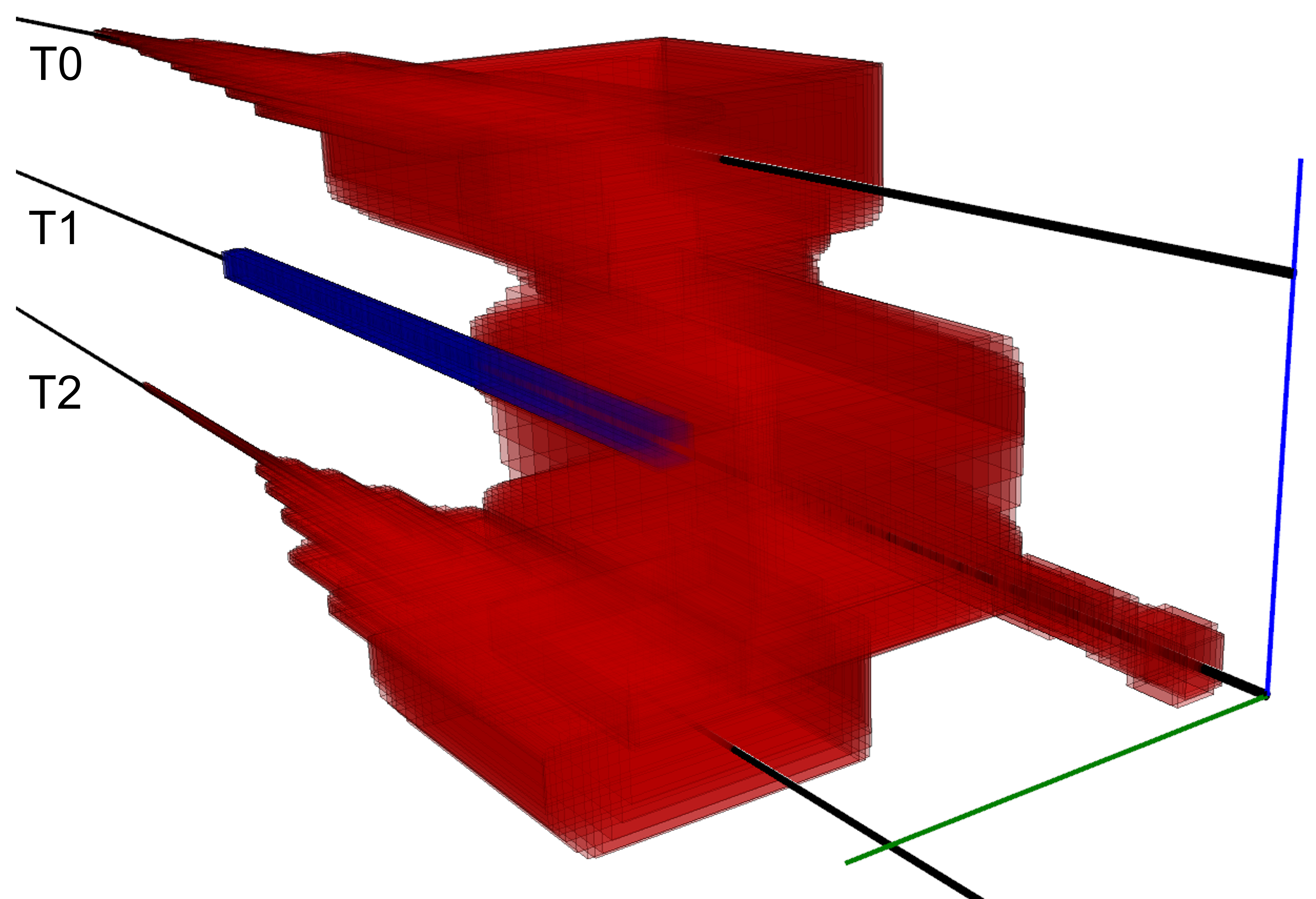
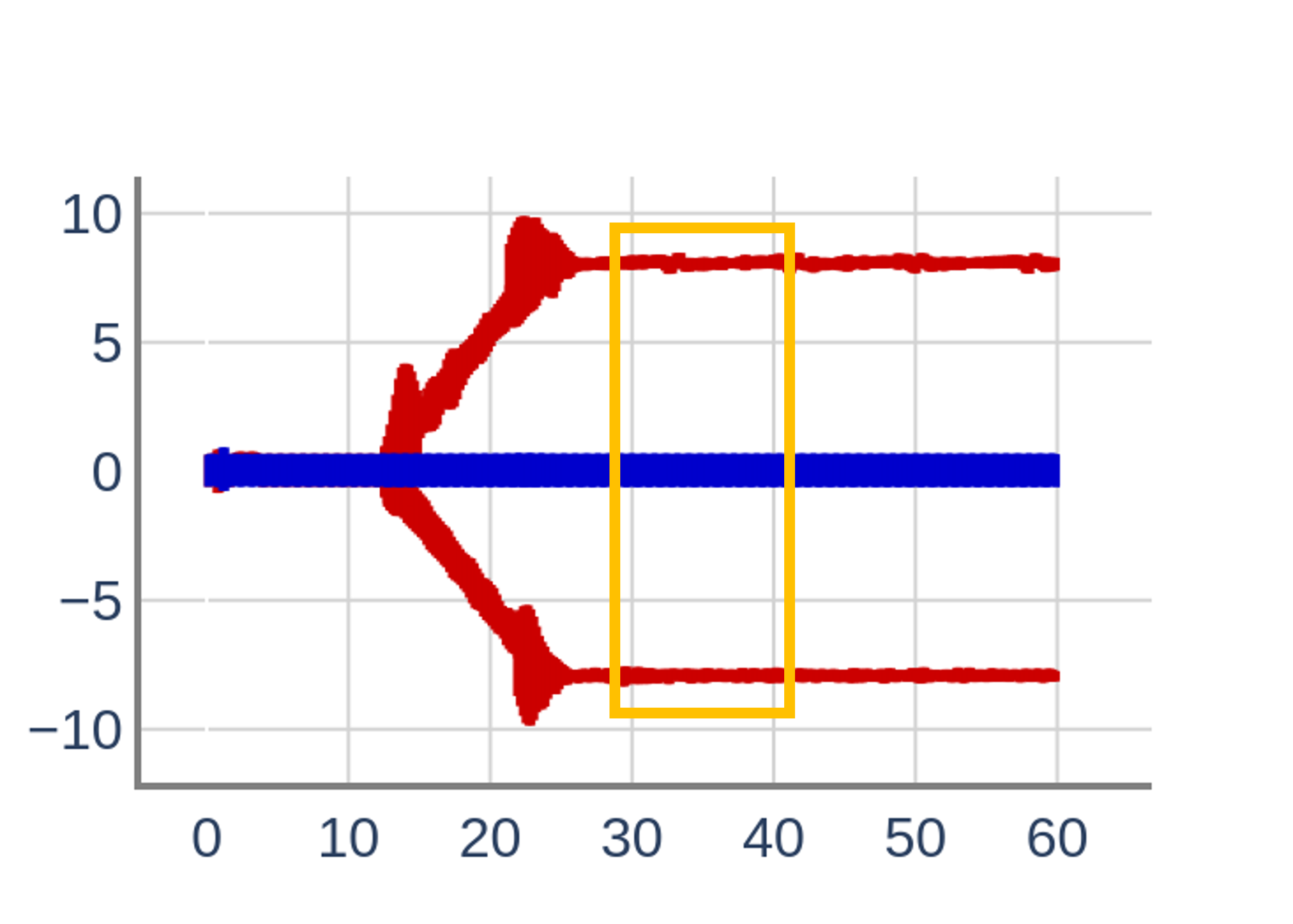
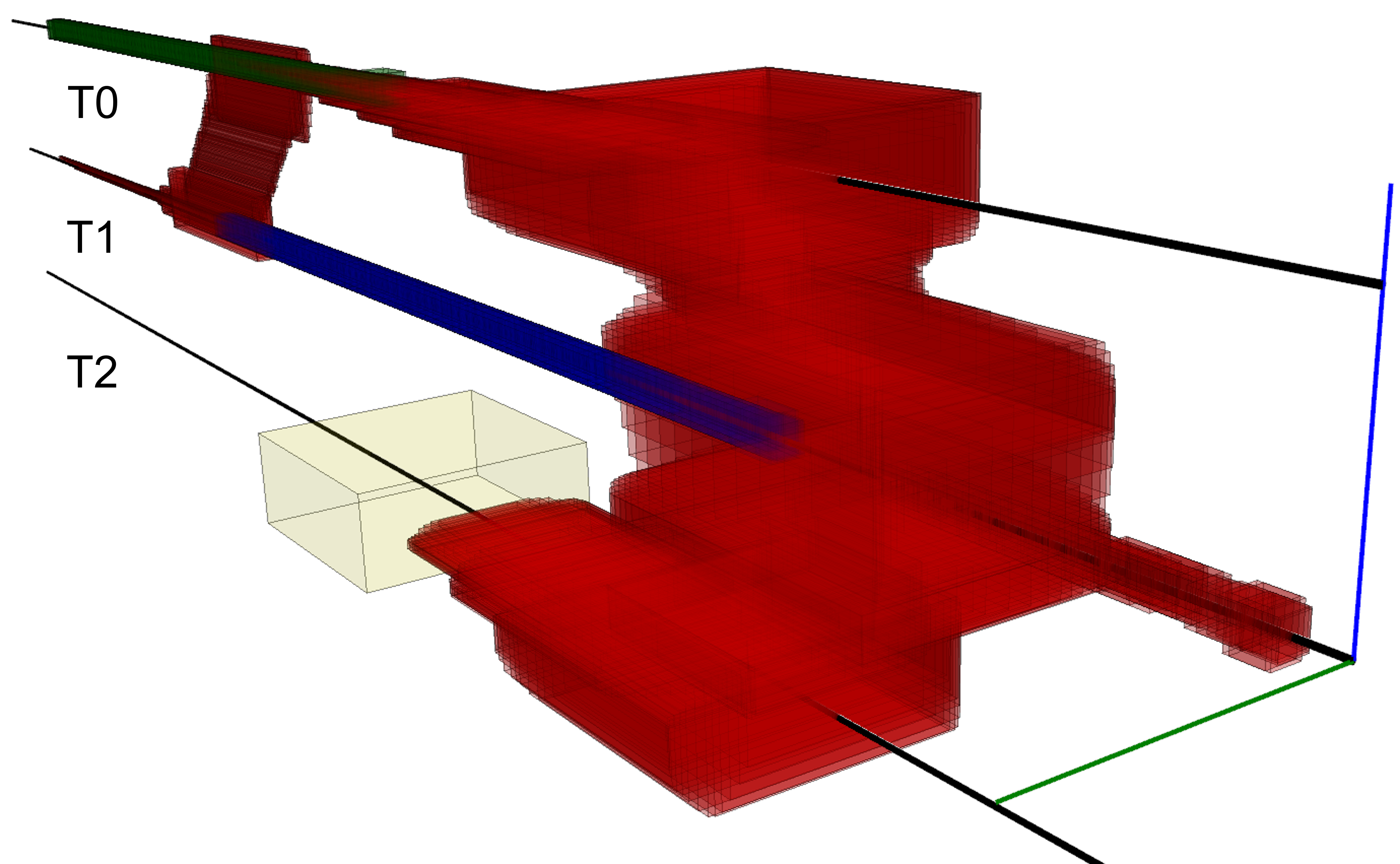
Figure 4: Left to right: (1) Computed reachtubes for a 2-drone scenario; (2) same reachtube projected on x-dimension, and (3) on z-dimension. Since there is no overlap in space-time, no collision. (4) Reachtube for a 3-drone scenario, the red drone violates the safety condition by entering the unsafe region after moving downward.

Checking multiple safety assertions.

Verse supports multiple safety assertions specified using assert statements. For example, the user can specify unsafe regions (Line 77-80) or check safe separation between agents (Line 81-83) as shown in Fig. 5. We extend the two-drone scenario described in the previous paragraph by adding a second D-NPV and both safety assertions. The result is shown in the rightmost Fig. 4. In this scenario, D-CA violates the safety property by entering the unsafe region after moving downward to avoid collision. The behavior of D-CA after moving upward is not influenced. There’s no violation of safe separation between agents in this scenario. Verse allow users to extract set of reachable states and mode transitions that leads to a safety violation.

⬇

from enum import Enum, auto

import copy

from typing import List

class CraftMode(Enum):

Normal = auto()

MoveUp = auto()

MoveDown = auto()

class TrackMode(Enum):

T0 = auto()

T1 = auto()

T2 = auto()

M01 = auto()

M10 = auto()

M12 = auto()

M21 = auto()

class State:

x: float

y: float

z: float

vx: float

vy: float

vz: float

craft_mode: CraftMode

track_mode: TrackMode

def __init__(self, x, y, z, vx, vy, vz, craft_mode, track_mode):

pass

def safe_seperation(ego, other):

res = ego.x-other.x < 1 and ego.x-other.x >-1 and \

ego.y-other.y < 1 and ego.y-other.y > -1 and \

ego.z-other.z < 1 and ego.z-other.z > -1

return res

def is_close(ego, other):

res = ((other.x - ego.x < 10 and other.x-ego.x > 8) or\

(other.y-ego.y < 10 and other.y-ego.y > 8) or\

(other.z-ego.z < 10 and other.z-ego.z > 8))

return res

def controller(ego: State, others: List[State], lane_map):

next = copy.deepcopy(ego)

if ego.craft_mode == CraftMode.Normal:

if any((is_close(ego, other) and ego.track_mode == other.track_mode) for other in others):

if lane_map.h_exist(ego.track_mode, ego.craft_mode, CraftMode.MoveUp):

next.craft_mode = CraftMode.MoveUp

next.track_mode = lane_map.h(

ego.track_mode, ego.craft_mode, CraftMode.MoveUp)

if lane_map.h_exist(ego.track_mode, ego.craft_mode, CraftMode.MoveDown):

next.craft_mode = CraftMode.MoveDown

next.track_mode = lane_map.h(

ego.track_mode, ego.craft_mode, CraftMode.MoveDown)

if ego.craft_mode == CraftMode.MoveUp:

if lane_map.altitude(ego.track_mode)-ego.z > -1 and lane_map.altitude(ego.track_mode)-ego.z < 1:

next.craft_mode = CraftMode.Normal

if lane_map.h_exist(ego.track_mode, ego.craft_mode, CraftMode.Normal):

next.track_mode = lane_map.h(

ego.track_mode, ego.craft_mode, CraftMode.Normal)

if ego.craft_mode == CraftMode.MoveDown:

if lane_map.altitude(ego.track_mode)-ego.z > -1 and lane_map.altitude(ego.track_mode)-ego.z < 1:

next.craft_mode = CraftMode.Normal

if lane_map.h_exist(ego.track_mode, ego.craft_mode, CraftMode.Normal):

next.track_mode = lane_map.h(

ego.track_mode, ego.craft_mode, CraftMode.Normal)

assert not (ego.x > 40 and ego.x<50 and\

ego.y>-5 and ego.y<5 and ego.z > -10 and ego.z<-6), "Unsafe Region"

assert not any(ego.x-other.x < 1 and ego.x-other.x >-1 and \

ego.y-other.y < 1 and ego.y-other.y > -1 and \

ego.z-other.z < 1 and ego.z-other.z > -1 \

for other in others), "Safe Separation"

return next

Figure 5: Safety assertions for three drone scenario.

Changing maps.

Verse allows users to easily create scenarios with different maps and port agents across compatible maps. We start with a scenario with one C-CA agent (red) and two C-NPV agents (blue, green) in $\mathcal{M}1$. The safety assertion is that the vehicles should be at least 1m apart in both $x$ and $y$-dimensions. Fig. 6 (left) shows the verification result and safety is not violated. However, if we switch to map $\mathcal{M}3$ by changing one line in the scenario definition, a reachability analysis shows that a safety violation can happen after C-CA merges left Fig. 6 (center). In addition, Verse allows importing map from OpenDRIVE [5] format, which enables users to easily create scenarios with interesting maps. An example is shown in Fig. 8 in Appendix.

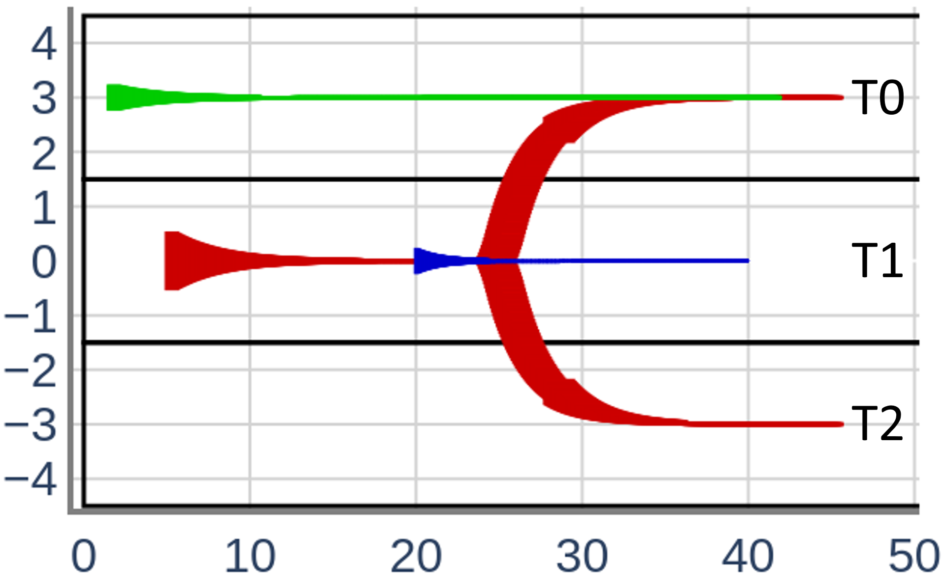
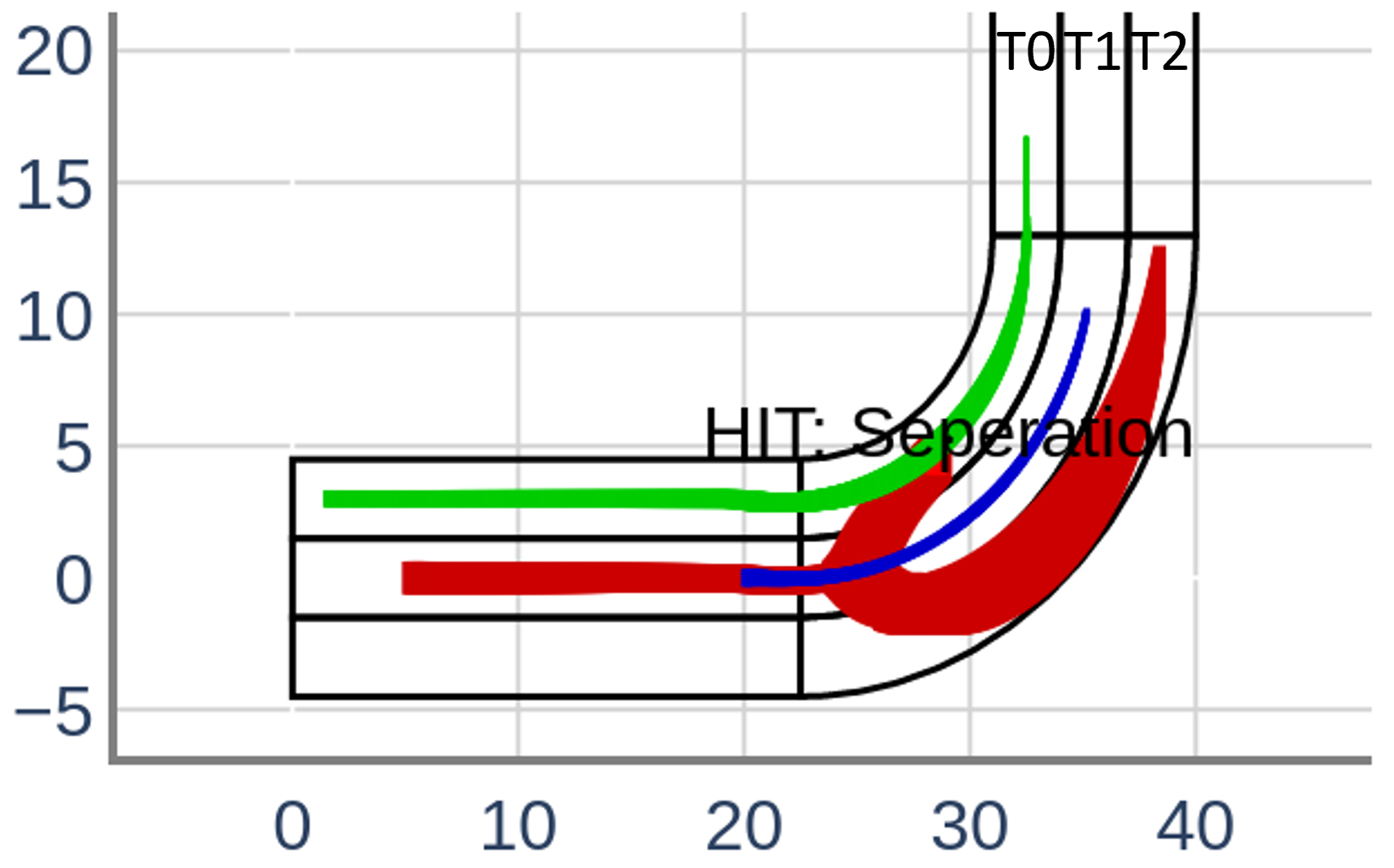
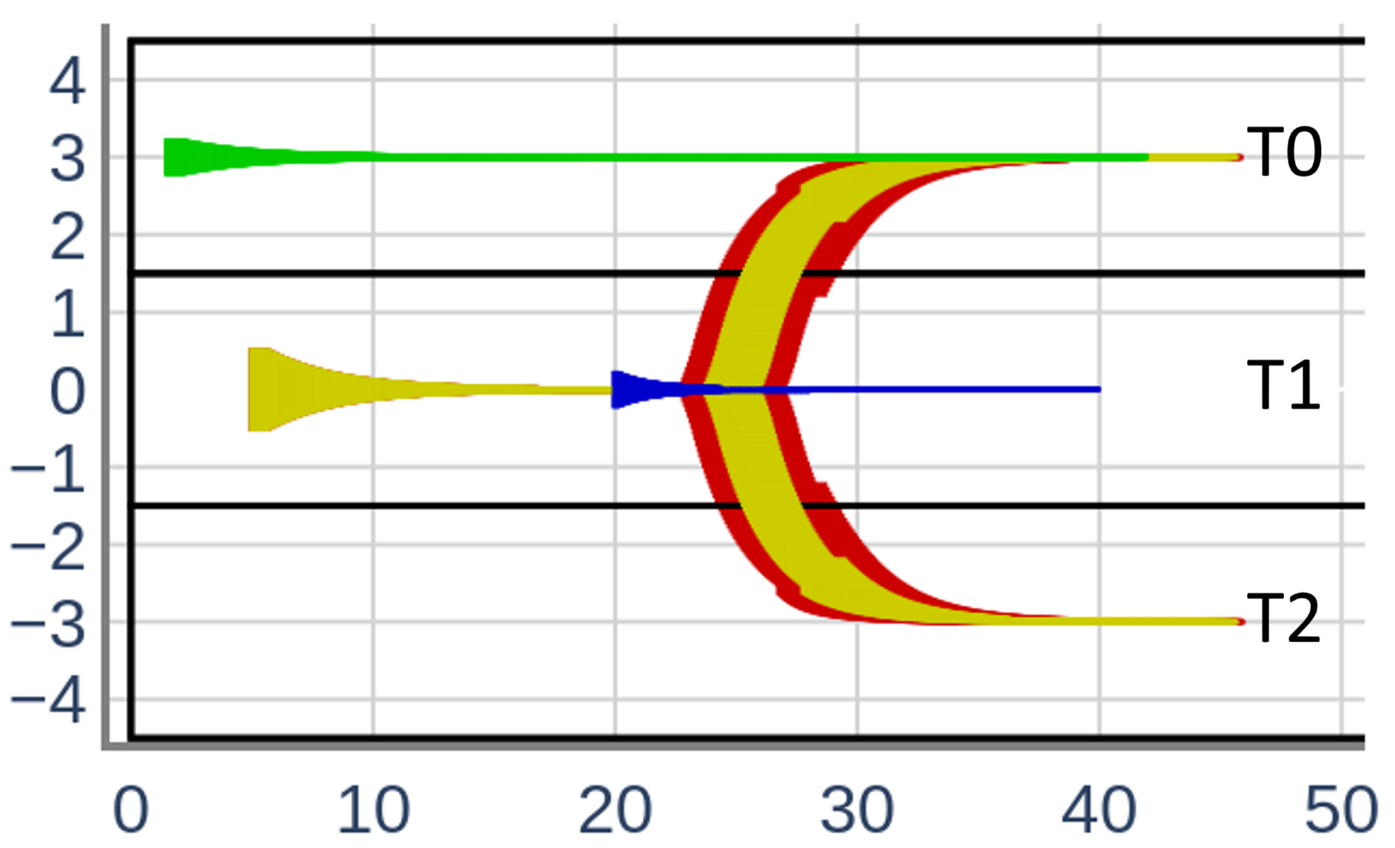
Figure 6: Left: running the three car scenario on map with parallel straight lanes. Center: same scenario with a curved map. Right: same scenario with a noisy sensor.

Adding noisy sensors.

Verse supports the ability to verify scenarios with different sensor functions. For example, the user can create a noisy sensor function that mimics a realistic sensor with bounded noise. Such sensor functions are easily added to the scenario using the set_sensor Verse library function.

Fig. 6 shows exactly the same three-car scenario as in the previous paragraph but with a noisy sensor, which adds $\pm 0.5m$ noise to the perceived position of all other vehicles. Since the sensed values of other agents only impacts the checking of the guards (and hence the transitions) of the ego agent, Verse internally bloats the reachable set of positions for the other agents by $\pm 0.5$ while checking guards. Compared with the behavior of the same agent with no sensor noise (shown in yellow in Fig 6 (right)), the sensor noise enlarges the region over which the transition can happen, which results in enlarged reachtubes for the red agent.

Plugging in different reachability engines.

With a little effort, Verse allows users to plug-in different reachability tools for the postCont computation. The user will need to modify the interface of the reachability tool so that given a set of initial states, a mode, and a non negative value $\delta$, the reachability tool can output the set of reachable states over a $\delta$-period represented by a set of timed hyperrectangles. Currently, Verse implements computing postCont using DryVR [12], NeuReach [33] and Mixed Monotone Decomposition [11]. A scenario with two car agents in map $\mathcal{M}1$ verified using NeuReach and DryVR is shown in Fig. 9 in the Appendix.

Table 1 summarizes the running time of verifying all the examples in this section on a standard Intel Core i7-11700K @ 3.60GHz CPU desktop. As expected, the running times increase with the number of discrete mode transition. However, for complicated scenario with $7$ agents and $37$ transitions, the verification can still finish in under $6$ mins, which suggests some level of scalability. The choice of reachability engine can also impact running time. For the same scenario in rows 2,3 and 10,11, Verse with NeuReach as the reachability engine takes more time than using DryVR as the reachability engine.

Table 1: Runtime for verifying examples in Section 6.1. Columns are: number of agents (#$\mathcal{A}$), agent type ($\mathcal{A}$), map used (Map), reachability engine used (postCont), sensor type (Noisy $\mathcal{S}$), number of mode transitions #TR, and the total run time (Run time).

#$\mathcal{A}$	$\mathcal{A}$	Map	postCont	Noisy $\mathcal{S}$	#Tr	Run time (s)
2	Q	$\mathcal{M}6$	DryVR	No	8	55.9
2	Q	$\mathcal{M}5$	DryVR	No	5	18.7
2	Q	$\mathcal{M}5$	NeuReach	No	5	1071.2
3	Q	$\mathcal{M}5$	DryVR	No	7	39.6
7	C	$\mathcal{M}2$	DryVR	No	37	322.7
3	C	$\mathcal{M}1$	DryVR	No	5	23.4
3	C	$\mathcal{M}3$	DryVR	No	4	34.7
3	C	$\mathcal{M}4$	DryVR	No	7	118.3
3	C	$\mathcal{M}1$	DryVR	Yes	5	29.4
2	C	$\mathcal{M}1$	DryVR	No	5	21.6
2	C	$\mathcal{M}1$	NeuReach	No	5	914.9

6.2 Incremental Verification

The incremental verification algorithm verifyInc is evaluated by repeatedly verifying (and simulating) scenarios with slight modifications. In this example, the scenario contains 3 C-CA agents and 5 C-NPV agents in map $\mathcal{M}2$. The simulation and verification results for the scenario are shown in Fig. 12 in Appendix 0.C. The running time for simulation is 19.96s and that for verification is 470.01s. We show the results for 3 experiments for both simulation and verification, which corresponds to the 3 rows in each section of Table 2. In the repeat experiments, we perform analysis twice on the same scenarios (${H}_{2}={H}_{1}$), which shows the most favorable benefits of incremental verification. In the change init and change ctlr experiments, we respectively change the initial conditions and the decision logic for one of the C-CA agents between the 2 experiment runs. We perform each of these experiments with incremental verification turned off and on, which corresponds to the verify and verifyInc columns.

From the experimental results we can see that verifyInc indeed reduces the time needed for simulation and verification. This time reduction is also correlated with the similarity between the scenarios, with the repeat experiment being able to achieve an almost 10x speedup, while changing the initial conditions leads to almost no benefit.

Table 2: Experimental results for the Incremental Verification algorithm. The table shows the number of mode transition (#Tr), run-times in seconds (run time), the memory usage of Verse in megabytes (memory), the size of ${C_{g}}$ and ${C_{f}}$ in megabytes (cache size), and the hit rate of the caches (hit rate).

			verify		verifyInc
		#Tr	run time	memory	Run time	memory	cache size	hit rate
Simulation	repeat	45	12.18	431	1.05	435	3.83	83.33%
	change init	24	10.17	431	9.3	436	4.07	75.91%
	change ctlr	45	11.45	429	5.98	438	4.38	78.19%
Verification	repeat	105	450.89	498	55.34	482	3.23	76.79%
	change init	49	365.91	485	349.68	498	3.7	73.21%
	change ctlr	93	421.65	498	230.12	490	4.0	73.44%

6.3 White-box uncertain continuous dynamics

Verse provides an implementation of postCont using algorithms from [1, 2, 11] which is applicable to agents with white-box uncertain continuous dynamics. Given a white-box dynamical system defined by a differential equation $\dot{x}=f(x,w)$, where the state $x\in\mathcal{X}\subseteq{\mathbb{R}}^{n}$ and the bounded disturbance input $w\in[w_{l},w_{u}]$. The idea of the approach in [11] is to find a decomposition function $d()$ which can then be used to define an augmented system:

$$\begin{bmatrix}\dot{x}_{l}\\ \dot{x}_{u}\end{bmatrix}=\begin{bmatrix}d(x_{l},w_{l},x_{u},w_{u})\\ d(x_{u},w_{u},x_{l},w_{l})\end{bmatrix},$$

such that the reachable set of the original noisy system at time $T$, from any initial set $\mathcal{X}_{0}=[\underline{x},\overline{x}]\subseteq\mathcal{X}$ is contained in $[{x_{l}}(T),{x_{u}}(T)]$. The latter can be computed by simulating the decomposed system from the singleton initial state $\langle x_{l}=\underline{x},x_{u}=\overline{x}\rangle$. Verse currently requires users to provide the decomposition function $d()$ to handle systems with uncertainty in dynamics. Consider an example system and the corresponding manually derived decomposition function: $$\begin{split}&\dot{x}_{1}=x_{1}(1.1+w_{1}-x_{1}-0.1x_{2})\\ &\dot{x}_{2}=x_{2}(4+w_{2}-3x_{1}-x_{2})\end{split}$$ $$d(x,\hat{x},w,\hat{w})=\begin{bmatrix}x_{1}(1.1+w_{1}-x_{1}-0.1\hat{x}_{2})\\ x_{2}(4+w_{2}-3\hat{x}_{1}-x_{2})\end{bmatrix}$$

With $x_{1},x_{2}\in[0.3,2]$ and $w_{1},w_{2}\in[-0.1,0.1]$. Verse can automatically construct the augmented system and compute the reachable states for that system (Sample results are shown in Fig. 10 of Appendix 0.C).

7 Conclusions and future directions

In this paper, we presented the new open source Verse library for broadening applications of hybrid system verification technologies to scenarios involving multiple interacting decision-making agents. Verse allows users to create agents with decision logics expressed in Python, scenarios with different types of agents, and it provides functions for performing systematic simulation and verification through reachability analysis. Verse maps can be imported from a standard open format, and they allow agents to be ported across different compatible maps, offering flexibility in creating scenarios. The agent decision logics allow non-deterministic decision making and the reachability functions can propagate the uncertainty in the initial condition through all decision branches. The safety requirements written using assert statements enable various safety conditions. The incremental verification algorithm in Verse enables the user to rapidly verify and improve their decision logic. We illustrate useful capabilities and use cases of Verse through various examples.

There are several exciting future directions for and around Verse. Verse currently assumes all agents interact with each other only through the sensor in the scenario and all agents share the same sensor. This restriction could be relaxed to have different types of asymmetric sensors. In incremental verification (and simulation), our verifyInc merely opens the door for a invention that exploit small changes in maps and continuous dynamics. Functions for constructing and systematically sampling scenarios could be developed. Functions for post-computation for white-box models by building connections with existing tools [3, 9, 13] would be a natural next step. Those approaches could obviously utilize the symmetry property of agent dynamics as in [30, 32], but beyond that, new types of symmetry reductions should be possibile by exploiting the map geometry.

Appendix 0.A Example Maps

The figure for maps used in the examples in Section 6 are shown in Fig. 7.

(a) $\mathcal{M}1$

(b) $\mathcal{M}2$

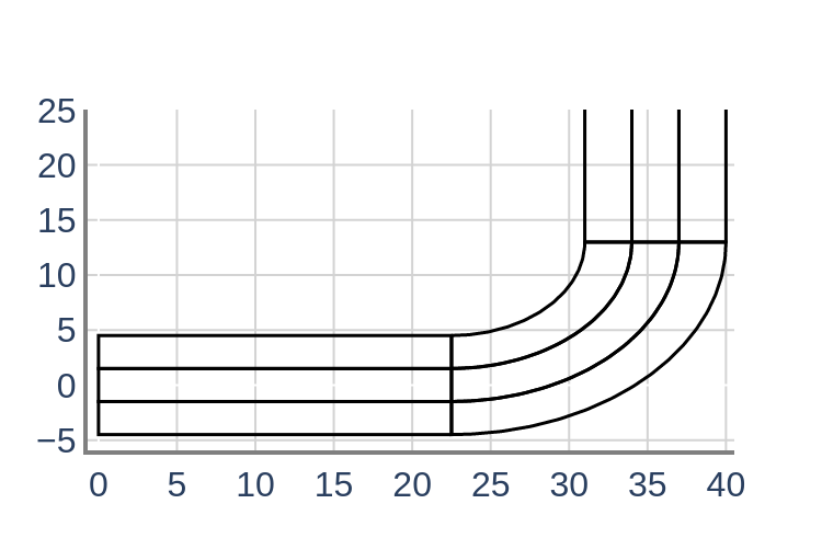
(c) $\mathcal{M}3$

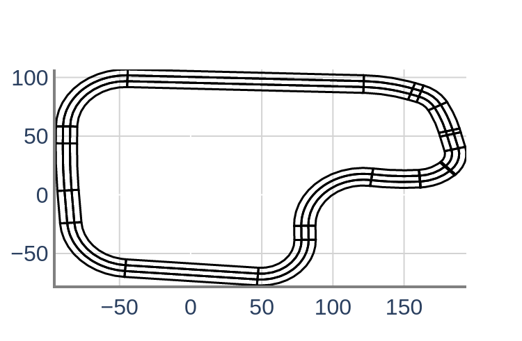
(d) $\mathcal{M}4$

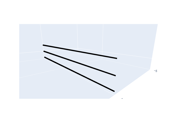
(e) $\mathcal{M}5$

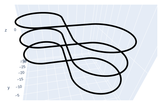
(f) $\mathcal{M}6$

Figure 7: Maps in examples

Appendix 0.B Grammar for Decision Logic Code

This is the subset of the Python grammar [28] that Verse support for coding the decision logic of agents. Some details about operator precedence are not given here. Currently, the supported OPERATOR include logic operators (and, or, and not), comparison operators (<=, <, ==, !=, >, and >=), and arithmetic operators (+, -, * and /).

⬇

expression:

| expression OPERATOR expression

| ’lambda’ parameters ’:’ expression

| literal

| dotted_name tuple

literal:

| [’-’] NUMBER

| STRING+

| ’None’ | ’True’ | ’False’

| tuple | group | genexp

expressions: ’,’.expression*

tuple: ’(’ expressions ’)’

group: ’(’ expression ’)’

genexp: ’(’ expression for_if_clauses+ ’)’

for_if_clause: ’for’ IDENT ’in’ expression (’if’ expression )*

function_def: ’def’ IDENT ’(’ [params] ’)’ [’->’ expression ] ’:’ block

params: (maybe_typed_name ’,’)* maybe_typed_name?

maybe_typed_name: IDENT [’:’ (expression | STRING)]

block:

| NEWLINE INDENT statements DEDENT

| simple_stmts

statements: statement+

statement: compound_stmt | simple_stmts

statement_newline: compound_stmt NEWLINE | simple_stmts | NEWLINE | EOF

compound_stmt: function_def | if_stmt | class_def

simple_stmts: ’;’.simple_stmt+ [’;’] NEWLINE

simple_stmt: assignment | return_stmt | assert_stmt | if_stmt

assignment: IDENT ’=’ expression

return_stmt: ’return’ [expression]

assert_stmt: ’assert’ expression [’,’ expression ]

if_stmt: ’if’ expression ’:’ block [else_block]

else_block: ’else’ ’:’ block

dotted_as_names: ’,’.dotted_as_name+

dotted_as_name: dotted_name [’as’ NAME ]

dotted_name: dotted_name ’.’ NAME | NAME

\par

Appendix 0.C Additional Examples

The verification result for a 3-car scenario with a map imported from OpenDRIVE format is shown in Fig. 8.

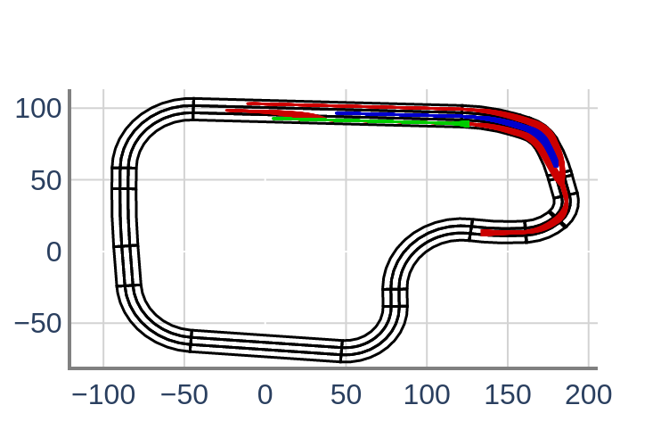
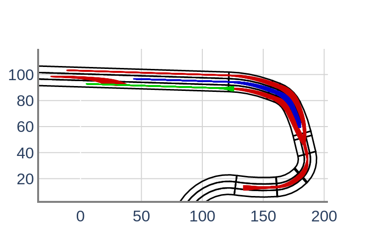
Figure 8: Picture showing verification result for a scenario with map imported from OpenDRIVE format.

The verification result with postCont computed by NeuReach and DryVR is shown in Fig. 9.

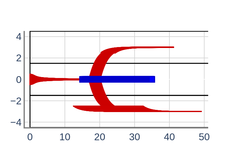
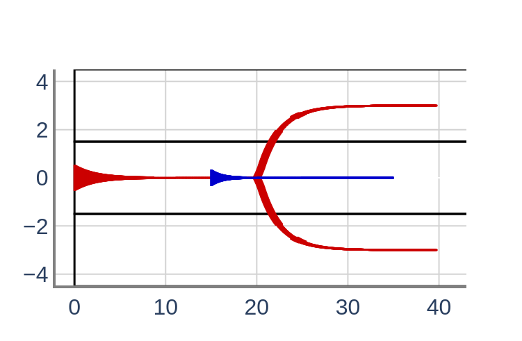
Figure 9: Picture on the left showing scenario with postCont computed by NueReach. Picture on the right showing same scenario with postCont computed by DryVR.

The ploted reachtube for $x_{1}$ and $x_{2}$ for system with uncertain dynamics in Section 6.3 is shown in Fig. 10.

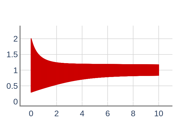
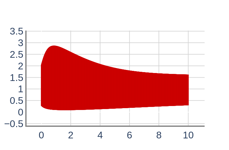
Figure 10: Reachtube plot for $x_{1}$ (left) and $x_{2}$ (right) for the example system.

The reachtube plot for the 7-car scenario described in row 5 of Table 1 is shown in Fig. 11.

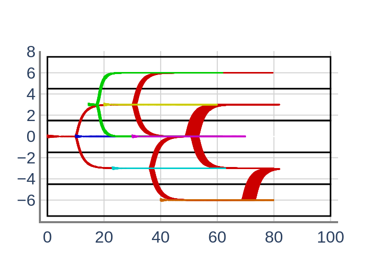
Figure 11: Reachtube plot for 7-car scenario

The simulation and verification result for the baseline 8-car system used for experimenting incremental verification in Section 6.2 is shown in Fig. 12

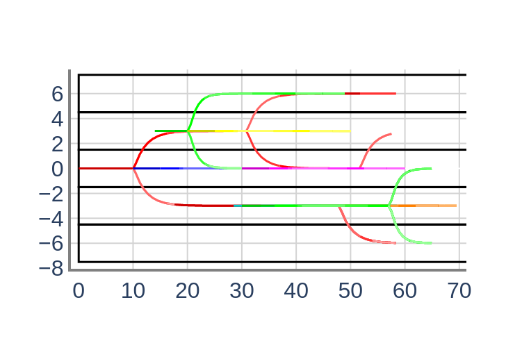
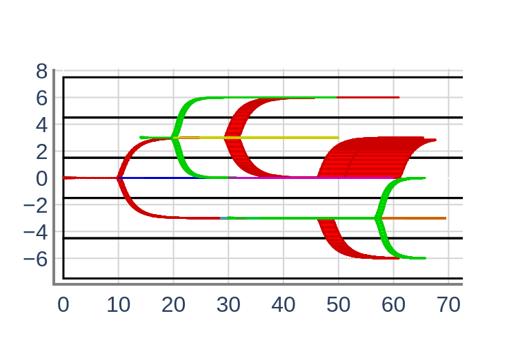
Figure 12: Simulation (left) and reachtube plot (right) for scenario in incremental verification experiment.

The baseline scenario for the incremental verification experiments is specified in Fig. 13 for simulation and in Fig. 14 for verification. In the change init experiment, the initial condition for car7 is changed to [[50, -3, 0, 0.5], [50, -3, 0, 0.5]]. In the change ctlr experiment, the controller for car8 is changed so that it switches tracks if there is another car less than 4.5 meters in front of it instead of 5 meters.

Figure 13: The scenario specification for the simulation baseline in the incremental verification experiments

⬇

scenario = Scenario()

controller_file = ’…’

car1 = CarAgent(’car1’, file_name=controller_file)

car1.set_initial([[0, 0, 0, 1.0], [0, 0, 0, 1.0]], (TacticalMode.Normal, TrackMode.T1))

scenario.add_agent(car1)

car2 = NPCAgent(’car2’)

car2.set_initial([[10, 0, 0, 0.5], [10, 0, 0, 0.5]], (TacticalMode.Normal, TrackMode.T1))

scenario.add_agent(car2)

car3 = CarAgent(’car3’, file_name=controller_file)

car3.set_initial([[14, 3, 0, 0.6], [14, 3, 0, 0.6]], (TacticalMode.Normal, TrackMode.T0))

scenario.add_agent(car3)

car4 = NPCAgent(’car4’)

car4.set_initial([[20, 3, 0, 0.5], [20, 3, 0, 0.5]], (TacticalMode.Normal, TrackMode.T0))

scenario.add_agent(car4)

car5 = NPCAgent(’car5’)

car5.set_initial([[30, 0, 0, 0.5], [30, 0, 0, 0.5]], (TacticalMode.Normal, TrackMode.T1))

scenario.add_agent(car5)

car6 = NPCAgent(’car6’)

car6.set_initial([[28.5, -3, 0, 0.5], [28.5, -3, 0, 0.5]], (TacticalMode.Normal, TrackMode.T2))

scenario.add_agent(car6)

car7 = NPCAgent(’car7’)

car7.set_initial([[39.5, -3, 0, 0.5], [39.5, -3, 0, 0.5]], (TacticalMode.Normal, TrackMode.T2))

scenario.add_agent(car7)

car8 = CarAgent(’car8’, file_name=controller_file)

car8.set_initial([[30, -3, 0, 0.6], [30, -3, 0, 0.6]], (TacticalMode.Normal, TrackMode.T2))

scenario.add_agent(car8)

Figure 14: The scenario specification for the verification baseline in the incremental verification experiments

⬇

scenario = Scenario()

controller_file = ’…’

car1 = CarAgent(’car1’, file_name=controller_file)

car1.set_initial([[0, -0.05, 0, 1.0], [0, 0.05, 0, 1.0]], (TacticalMode.Normal, TrackMode.T1))

scenario.add_agent(car1)

car2 = NPCAgent(’car2’)

car2.set_initial([[10, 0, 0, 0.5], [10, 0, 0, 0.5]], (TacticalMode.Normal, TrackMode.T1))

scenario.add_agent(car2)

car3 = CarAgent(’car3’, file_name=controller_file)

car3.set_initial([[14, 2.95, 0, 0.6], [14, 3.05, 0, 0.6]], (TacticalMode.Normal, TrackMode.T0))

scenario.add_agent(car3)

car4 = NPCAgent(’car4’)

car4.set_initial([[20, 3, 0, 0.5], [20, 3, 0, 0.5]], (TacticalMode.Normal, TrackMode.T0))

scenario.add_agent(car4)

car5 = NPCAgent(’car5’)

car5.set_initial([[30, 0, 0, 0.5], [30, 0, 0, 0.5]], (TacticalMode.Normal, TrackMode.T1))

scenario.add_agent(car5)

car6 = NPCAgent(’car6’)

car6.set_initial([[28.5, -3, 0, 0.5], [28.5, -3, 0, 0.5]], (TacticalMode.Normal, TrackMode.T2))

scenario.add_agent(car6)

car7 = NPCAgent(’car7’)

car7.set_initial([[39.5, -3, 0, 0.5], [39.5, -3, 0, 0.5]], (TacticalMode.Normal, TrackMode.T2))

scenario.add_agent(car7)

car8 = CarAgent(’car8’, file_name=controller_file)

car8.set_initial([[30, -3.05, 0, 0.6], [30, -2.95, 0, 0.6]], (TacticalMode.Normal, TrackMode.T2))

scenario.add_agent(car8)

The simulation and verification result for the 8-car system after changing initial condition is shown in Fig. 15. The agent with changed controller is marked with the red box in the plot.

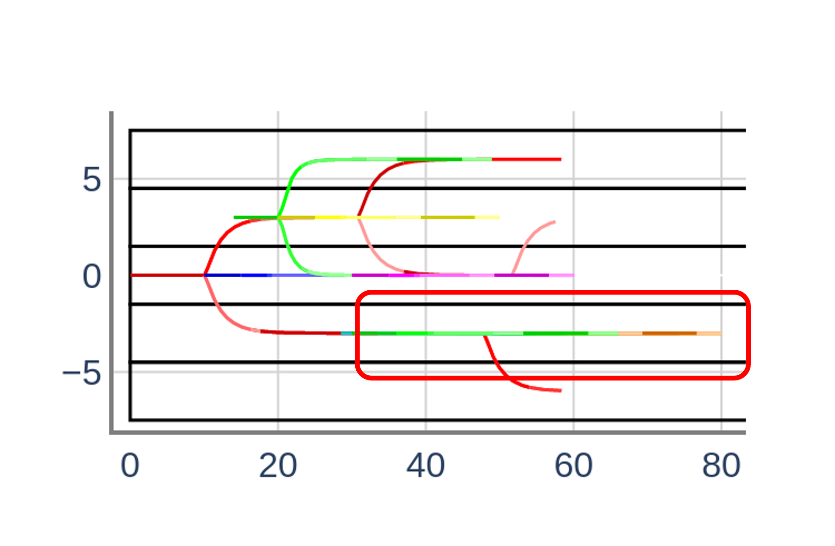
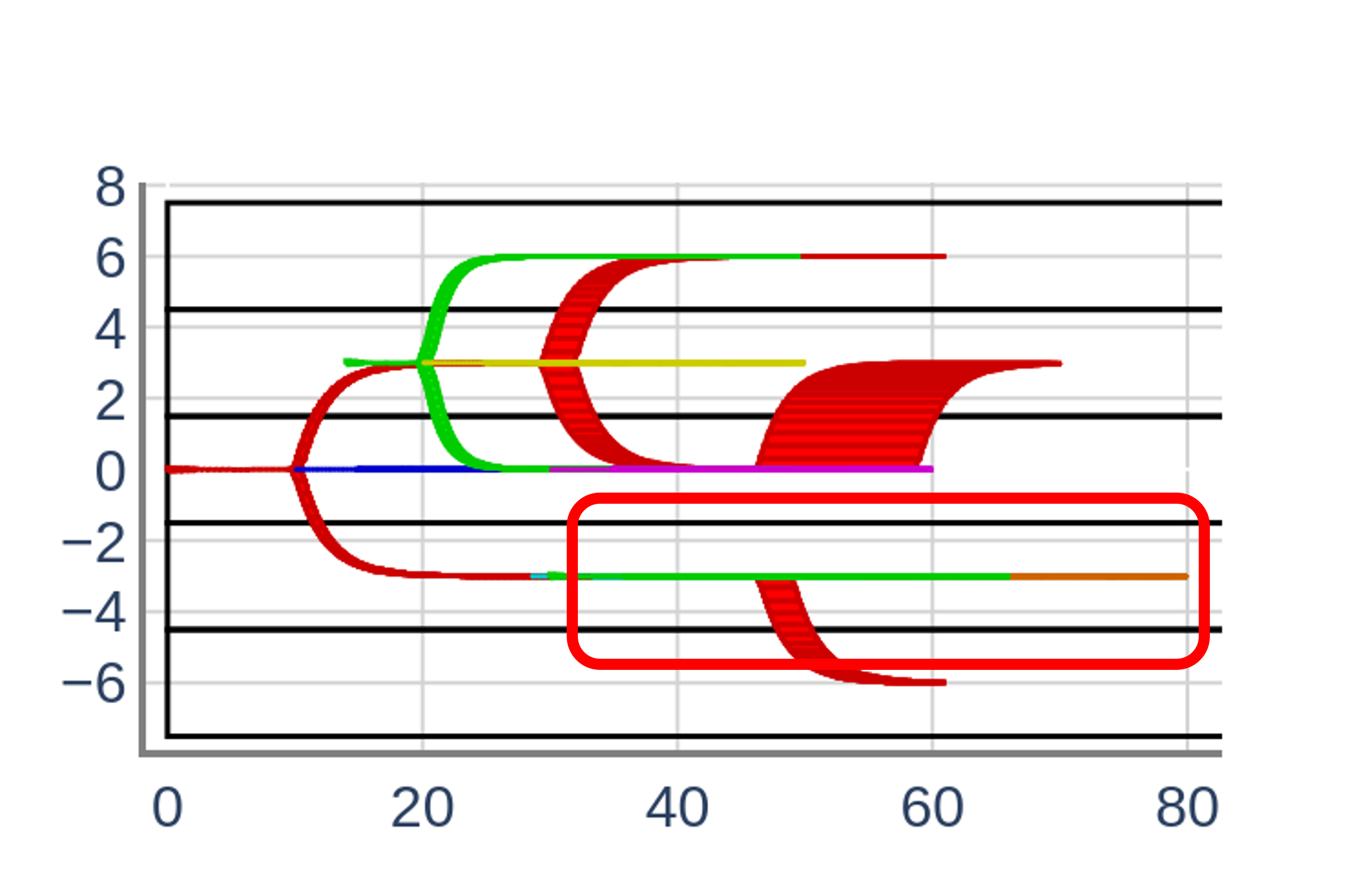
Figure 15: Simulation (left) and reachtube plot (right) for scenario after changing initial condition in incremental verification experiment.

The simulation and verification result for the 8-car system after changing controller is shown in Fig. 16. The agent with changed controller is marked with the red box in the plot.

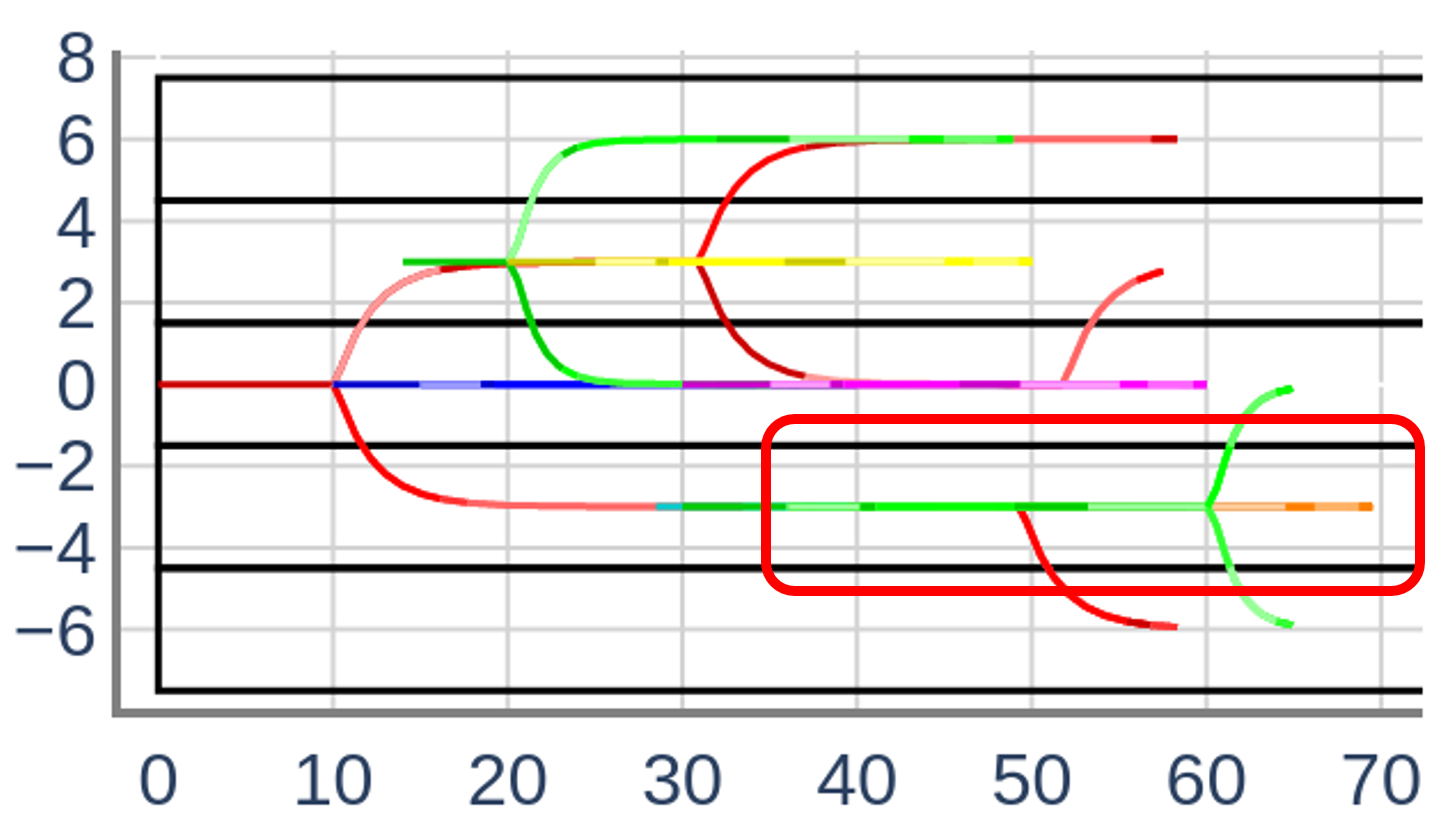
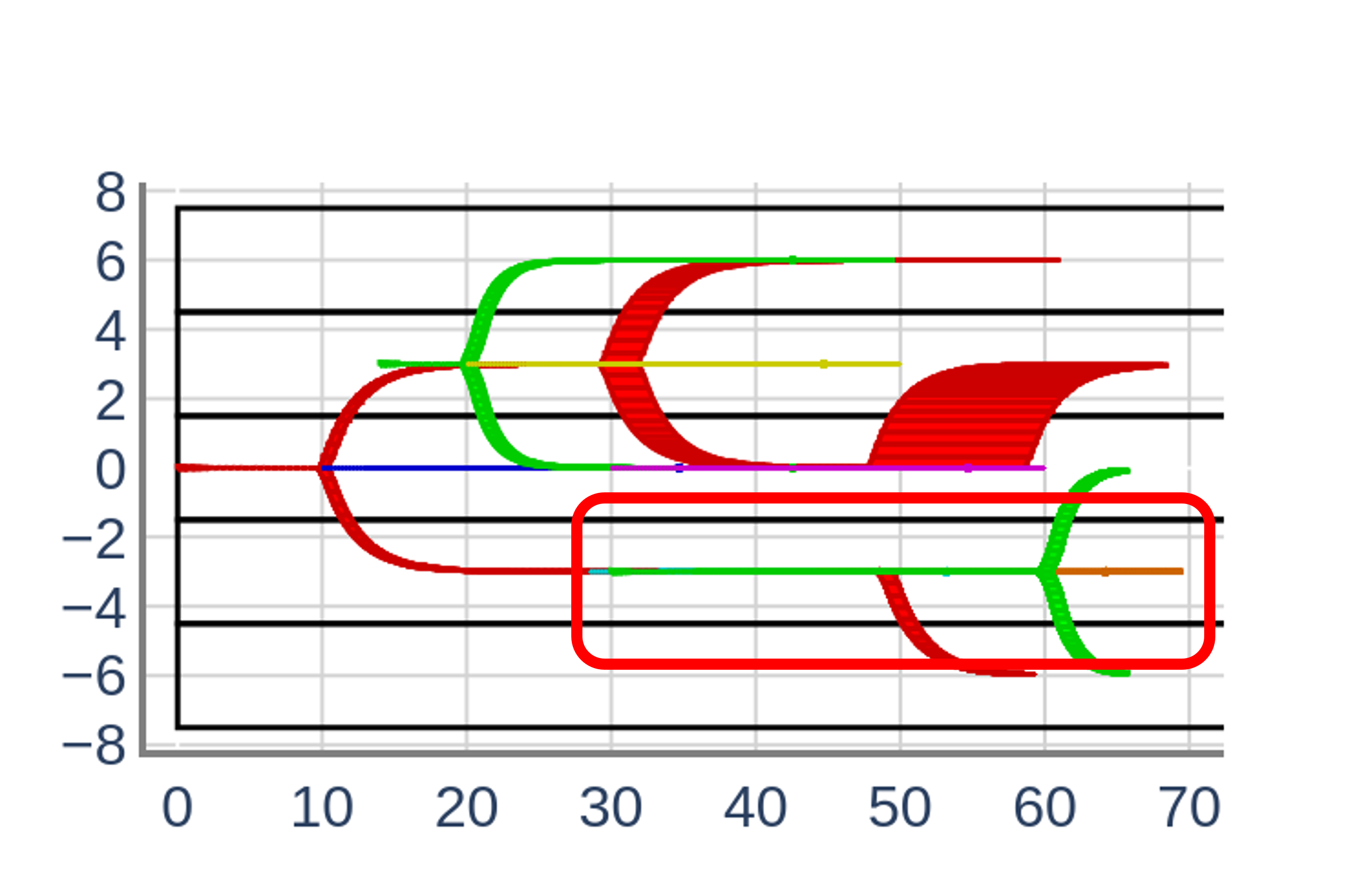
Figure 16: Simulation (left) and reachtube plot (right) for scenario after changing controller in incremental verification experiment.

References

- [1] Abate, M.: Mixed Monotonicity for Efficient Reachability with Applications to Robust Safe Autonomy. Ph.D. thesis, Georgia Institute of Technology (2020)
- [2] Abate, M., Coogan, S.: Computing robustly forward invariant sets for mixed-monotone systems. In: 2020 59th IEEE Conference on Decision and Control (CDC). pp. 4553–4559 (2020)
- [3] Althoff, M.: An introduction to CORA 2015. In: Proc. of the Workshop on Applied Verification for Continuous and Hybrid Systems (2015)
- [4] Alur, R., Courcoubetis, C., Halbwachs, N., Henzinger, T.A., Ho, P.H., Nicollin, X., Olivero, A., Sifakis, J., Yovine, S.: The algorithmic analysis of hybrid systems. Theoretical Computer Science 138(1), 3–34 (1995)
- [5] Association for Standardization of Automation and Measuring Systems (ASAM): Open dynamic road information for vehicle environment (Aug 2021), https://www.asam.net/standards/detail/opendrive/
- [6] Bak, S., Duggirala, P.S.: Hylaa: A tool for computing simulation-equivalent reachability for linear systems. In: Proceedings of the 20th International Conference on Hybrid Systems: Computation and Control. pp. 173–178. ACM (2017)
- [7] Bak, S., Tran, H.D., Johnson, T.T.: Numerical verification of affine systems with up to a billion dimensions. In: Proceedings of the 22nd ACM International Conference on Hybrid Systems: Computation and Control. p. 23–32. HSCC ’19, Association for Computing Machinery, New York, NY, USA (2019)
- [8] Brittain, M., Alvarez, L.E., Breeden, K., Jessen, I.: AAM-Gym: Artificial intelligence testbed for advanced air mobility (2022)
- [9] Chen, X., Ábrahám, E., Sankaranarayanan, S.: Flow*: An analyzer for non-linear hybrid systems. In: Computer Aided Verification (CAV). pp. 258–263. Springer (2013)
- [10] Chen, X., Sankaranarayanan, S.: Reachability analysis for cyber-physical systems: Are we there yet? In: Deshmukh, J.V., Havelund, K., Perez, I. (eds.) NASA Formal Methods. pp. 109–130. Springer, Cham (2022)
- [11] Coogan, S.: Mixed monotonicity for reachability and safety in dynamical systems. In: 2020 59th IEEE Conference on Decision and Control (CDC). pp. 5074–5085 (2020)
- [12] Fan, C., Qi, B., Mitra, S., Viswanathan, M.: Dryvr: Data-driven verification and compositional reasoning for automotive systems. In: Majumdar, R., Kunčak, V. (eds.) Computer Aided Verification (CAV). pp. 441–461. Springer, Cham (2017)
- [13] Fan, C., Qi, B., Mitra, S., Viswanathan, M., Duggirala, P.S.: Automatic reachability analysis for nonlinear hybrid models with C2E2. In: Computer Aided Verification (CAV). pp. 531–538 (2016)
- [14] Federal Aviation Administration: Unmanned Aircraft System Traffic Management (UTM) Concept of Operations Version 2.0 (Mar 2020)
- [15] Foster, S., Huerta y Munive, J.J., Gleirscher, M., Struth, G.: Hybrid systems verification with Isabelle/HOL: Simpler syntax, better models, faster proofs. In: Huisman, M., Păsăreanu, C., Zhan, N. (eds.) Formal Methods. pp. 367–386. Springer, Cham (2021)
- [16] Frehse, G., Guernic, C.L., Donzé, A., Cotton, S., Ray, R., Lebeltel, O., Ripado, R., Girard, A., Dang, T., Maler, O.: SpaceEx: Scalable verification of hybrid systems. In: Computer Aided Verification (CAV). pp. 379–395 (2011)
- [17] Fremont, D.J., Dreossi, T., Ghosh, S., Yue, X., Sangiovanni-Vincentelli, A.L., Seshia, S.A.: Scenic: A language for scenario specification and scene generation. In: Proceedings of the 40th ACM SIGPLAN Conference on Programming Language Design and Implementation. p. 63–78. PLDI 2019, Association for Computing Machinery, New York, NY, USA (2019)
- [18] Fulton, N., Mitsch, S., Quesel, J.D., Völp, M., Platzer, A.: KeYmaera X: An axiomatic tactical theorem prover for hybrid systems. In: Felty, A.P., Middeldorp, A. (eds.) Automated Deduction - CADE-25. pp. 527–538. Springer, Cham (2015)
- [19] Goldenberg, D.K., Lin, J., Morse, A.S.: Towards mobility as a network control primitive. In: MobiHoc ’04: Proceedings of the 5th ACM international symposium on Mobile ad hoc networking and computing. pp. 163–174. ACM Press (2004)
- [20] Henzinger, T.A., Kopke, P.W., Puri, A., Varaiya, P.: What’s decidable about hybrid automata? Journal of Computer and System Sciences 57(1), 94–124 (1998)
- [21] Hoffmann, G.M., Tomlin, C.J., Montemerlo, M., Thrun, S.: Autonomous automobile trajectory tracking for off-road driving: Controller design, experimental validation and racing. In: 2007 American Control Conference. pp. 2296–2301 (2007)
- [22] Ivanov, R., Weimer, J., Alur, R., Pappas, G.J., Lee, I.: Verisig: verifying safety properties of hybrid systems with neural network controllers. In: Proceedings of the 22nd ACM International Conference on Hybrid Systems: Computation and Control. pp. 169–178 (2019)
- [23] Kaynar, D.K., Lynch, N., Segala, R., Vaandrager, F.: The Theory of Timed I/O Automata. Synthesis Lectures on Computer Science, Morgan Claypool (November 2005), also available as Technical Report MIT-LCS-TR-917, MIT
- [24] Lim, H., Kaynar, D., Lynch, N., Mitra, S.: Translating timed I/O automata specifications for theorem proving in PVS. In: Proceedings of Formal Modelling and Analysis of Timed Systems (FORMATS’05). No. 3829 in LNCS, Springer, Uppsala, Sweden (September 2005)
- [25] Lopez, P.A., Behrisch, M., Bieker-Walz, L., Erdmann, J., Flötteröd, Y.P., Hilbrich, R., Lücken, L., Rummel, J., Wagner, P., Wießner, E.: Microscopic traffic simulation using SUMO. In: The 21st IEEE International Conference on Intelligent Transportation Systems. IEEE (2018)
- [26] Manfredi, G., Jestin, Y.: An introduction to ACAS Xu and the challenges ahead. In: 2016 IEEE/AIAA 35th Digital Avionics Systems Conference (DASC). pp. 1–9. IEEE (2016)
- [27] Minghao Jiang and Zexiang Liu and Kristina Miller and Dawei Sun and Arnab Datta and Yixuan Jia and Sayan Mitra and Necmiye Ozay: Graic: A simulator framework for autonomous racing. https://popgri.github.io/Race/ (2021)
- [28] Python Software Foundation: Python full grammar specification (Oct 2022)
- [29] Ray, R., Gurung, A., Das, B., Bartocci, E., Bogomolov, S., Grosu, R.: Xspeed: Accelerating reachability analysis on multi-core processors. In: Piterman, N. (ed.) Hardware and Software: Verification and Testing. pp. 3–18. Springer, Cham (2015)
- [30] Sibai, H., Li, Y., Mitra, S.: SceneChecker: Boosting scenario verification using symmetry abstractions (2021)
- [31] Sibai, H., Mokhlesi, N., Fan, C., Mitra, S.: Multi-agent safety verification using symmetry transformations. In: Biere, A., Parker, D. (eds.) Tools and Algorithms for the Construction and Analysis of Systems. pp. 173–190. Springer, Cham (2020)
- [32] Sibai, H., Mokhlesi, N., Mitra, S.: Using symmetry transformations in equivariant dynamical systems for their safety verification. In: Chen, Y.F., Cheng, C.H., Esparza, J. (eds.) Automated Technology for Verification and Analysis. pp. 98–114. Springer, Cham (2019)
- [33] Sun, D., Mitra, S.: Neureach: Learning reachability functions from simulations. In: Tools and Algorithms for the Construction and Analysis of Systems - 28th International Conference, TACAS 2022, Held as Part of the European Joint Conferences on Theory and Practice of Software, ETAPS 2022, Munich, Germany, April 2-7, 2022, Proceedings, Part I. pp. 322–337 (2022)
- [34] Wu, C., Kreidieh, A., Parvate, K., Vinitsky, E., Bayen, A.M.: Flow: Architecture and benchmarking for reinforcement learning in traffic control. ArXiv abs/1710.05465 (2017)
- [35] Ölveczky, P.C., Meseguer, J.: Specification of real-time and hybrid systems in rewriting logic. Theoretical Computer Science 285(2), 359–405 (2002), rewriting Logic and its Applications