Baechi: Fast Device Placement of Machine Learning Graphs

Abstract.

Machine Learning graphs (or models) can be challenging or impossible to train when either devices have limited memory, or models are large. To split the model across devices, learning-based approaches are still popular. While these result in model placements that train fast on data (i.e., low step times), learning-based model-parallelism is time-consuming, taking many hours or days to create a placement plan of operators on devices. We present the Baechi system, the first to adopt an algorithmic approach to the placement problem for running machine learning training graphs on small clusters of memory-constrained devices. We integrate our implementation of Baechi into two popular open-source learning frameworks: TensorFlow and PyTorch. Our experimental results using GPUs show that: (i) Baechi generates placement plans $654\times$–$206$K $\times$ faster than state-of-the-art learning-based approaches, and (ii) Baechi-placed model’s step (training) time is comparable to expert placements in PyTorch, and only up to 6.2% worse than expert placements in TensorFlow. We prove mathematically that our two algorithms are within a constant factor of the optimal. Our work shows that compared to learning-based approaches, algorithmic approaches can face different challenges for adaptation to Machine learning systems, but also they offer proven bounds, and significant performance benefits.

Introduction

Distributed Machine Learning frameworks use more than one device in order to train large models and allow for larger training sets. This has led to multiple open-source systems, including TensorFlow (Abadi et al., 2016), PyTorch (Paszke et al., 2019), MXNet (Chen et al., 2015), Theano (Theano Development Team, 2016), Caffe (Jia et al., 2014), CNTK (Seide and Agarwal, 2016), and others (Kraska et al., 2013; Sparks et al., 2013; Xing et al., 2015). Many of these systems use data parallelism, wherein each device (GPU) runs the entire model, and multiple items are inputted and trained in parallel across devices.

Yet, the increasing size of Machine Learning (ML) models and scale of training datasets is quickly outpacing available GPU memory. For instance the vanilla implementation of a 1000-layer deep residual network required 48 GB memory (Chen et al., 2016), which is much larger than the amount of RAM available on a typical COTS (Commercial Off-the-Shelf) device. Even after further optimizations to reduce memory cost, the ML model still required 7 GB memory, making it impossible to run an entire model on a single device with limited memory, as well as prohibitively expensive on public clouds like AWS (Amazon, 2022b), Google Cloud (Google, 2022), and Azure (Microsoft, 2022).

At the same time, today, ML training is gravitating towards being run among small collections of memory-constrained devices. These include small groups of cheap devices like edge devices (for scenarios arising from Internet of Things and Cyberphysical systems), Unmanned Aerial Vehicles (UAVs or drones), and to some extent even mobile devices. For instance, real-time requirements (Mahdavinejad et al., 2018; Zeydan et al., 2016), privacy needs (Bonawitz et al., 2017, 2019), or budgetary constraints, necessitate training only using nearby or in-house devices with limited resources.

These two trends—increasing model graph sizes and growing prevalence of puny devices being used to train the model graph—together cause scenarios wherein a single device is insufficient and results in an Out of Memory (or OOM) exception. For example, we found that the Google Neural Machine Translation (GNMT) (Wu et al., 2016) model OOMs on a 4 GB GPU even with conservative parameters: batch size 128, 4 512-unit long short-term memory (LSTM) layers, 30K vocabulary, and sequence length 50.

This problem is traditionally solved by adopting model parallelism, wherein the ML model graph is split across multiple devices. Today, a popular way to accomplish model parallelism in industry is to use learning-based approaches to generate the placement of operators on devices, most commonly by using Reinforcement Learning (RL) or variants. Significant in this space are works from Google (Mirhoseini et al., 2017, 2018) and the Placeto system (Addanki et al., 2019). A learning-based approach learns iteratively (via RL) and adjusts the placement on the target cluster, with the goal of minimizing execution time for each training step in the placed model, i.e., its step time.

While learning-based approaches achieve step times around those obtained by expert placements, they can unfortunately take an inordinately long time to generate their placement plans. For instance, using one state-of-the-art learning-based approach (Addanki et al., 2019), NMT models require 94,000 steps during the learning-based placement, and even with a conservatively low estimate of runtime per learning step of 2.63 seconds, the total placement time would come to 68.67 hours. One might possibly apply parallelization techniques (Jia et al., 2019, 2018; Wang et al., 2019a) to the learning model being used to perform placement, in order to speed it up, but the total incurred resource costs would stay just as high—hence, parallelization is orthogonal to our discussion.

Such long waits are cumbersome and even prohibitive at model development time, when the software developer needs to make many quick and ad-hoc deployments (Addanki et al., 2019). In fact, studies of analytics clusters reveal that most analytics job runs tend to be short (Wang et al., 2019b; Chen et al., 2012). For instance, the step time for a typical model graph (e.g., NMT or Inception-V3), to train on a single data batch, is O(seconds) on a typical GPU. Overwhelming this time with learning-based placement times which span hours, significantly inhibits the developer’s agility.

Additionally, a learning-based placement run works only for a target cluster and a given model graph with fixed hyperparameters (e.g., batch size, learning rate, etc.). If the model graph were to be transitioned to a different cluster with different GPU specs, the learning has to be repeated all over again, incurring the high overhead. Consider a developer who is trying to find the right batch size for a target cluster. This process of exploration is iterative, and every hyperparameter value trial needs a new run of the learning-based technique, making the overall undertaking slow.

For the model development process to be agile, nimble, and at the same time coherent with future real deployments, what is needed is a new class of placement techniques for model parallelism, that: i) are significantly faster in placement than learning-based approaches, and yet ii) achieve fast step times in the placed model.

This paper is the first to adopt a traditional algorithmic approach for the placement of ML models on memory-constrained clusters. Subsequent to our initial work (Jeon et al., 2020), a few other authors have published algorithmic or dynamic programming-based ideas for model placement, however these are either : i) standalone and not integrated into open-source systems (Tarnawski et al., 2020), ii) or they are aimed at only placing specific models like transformers (Li et al., 2021), (Shoeybi et al., 2019), or iii) they are at best comparable in performance to ours (Hafeez et al., 2021). Orthogonal to model parallelism is pipeline parallelism (Harlap et al., 2018),(Huang et al., 2019),(Fan et al., 2021),(Yang et al., 2021)—our paper does not explore the latter, in order to keep our discussion focused on the benefits of algorithmic approaches over learning approaches.

The contributions of this paper are:

• We adapt classical literature from parallel job scheduling to propose two memory-constrained algorithms, called m-SCT (memory-constrained Small Communication Times) and m-ETF (memory-constrained Earliest Task First). We also present m-TOPO (memory-constrained TOPO-logical order), a strawman. We focus on the static version of the problem.

• We prove that under certain assumptions, both m-ETF and m-SCT steps time is within a constant factor of the optimal.

• We present the Baechi system (Korean for placement, pronounced “Bay-Chee”). Baechi incorporates m-SCT/m-ETF into both TensorFlow as well as PyTorch. Our exposition focuses on the multiple design decisions that were needed in Baechi to derive performance out of the algorithmic underpinnings.

• We present tailored integration of Baechi with both TensorFlow and PyTorch to address the different programming abstractions and architecture in these two frameworks.

• We present experimental results from a real deployment on a small cluster of GPUs, using both TensorFlow and PyTorch which show that Baechi generates placement plans in time $654\times$–$206$K $\times$ faster than today’s learning-based approaches, and yet the placed model’s step time (training time) is either faster than or, at worst, only up to 6.2% higher, compared to expert-based placements.

New Algorithms for Memory-Constrained Placement

This section presents the problem formulation and our three placement techniques. For each technique, we first discuss the classical approach (not memory-aware), and then our adapted memory-constrained algorithm. Where applicable, we prove optimality.

Our three approaches are: 1) a placer based on topological sorting (TOPO) 2) a placer based on Earliest Task First (ETF), and 3) a placer based on Small Communication Time (SCT).

Problem Formulation

Given $n$ devices (GPUs), each with memory size $M$, and a Machine Learning (ML) graph $G$ that is a DAG (Directed Acyclic Graph) of operators, the device placement problem is to place nodes of $G$ (operators) on the devices so that the makespan is minimized. Makespan, equivalent to step time, is traditionally defined as the total execution time to train on one input mini-batch (i.e., unit of training data). Table 1 summarizes key terms used throughout the paper. When discussing classical algorithms, we use the classical terms “tasks” instead of operators.

If one assumes devices have infinite (sufficient) memory, scheduling with communication delay is a well-studied theoretical problem. The problem is NP-hard even when under the simplest of assumptions (Hoogeveen et al., 1994), such as infinite number of devices and unit times for computation and communication (UET-UCT).

Out of the three best-performing solutions to the infinite memory problem, we choose the two that map best to ML graphs: 1) Earliest Task First or ETF  (Veltman et al., 1990; Hwang et al., 1989), and 2) Small Communication Time or SCT (Hanen and Munier, 1995). SCT is provably close to optimal when the ratio of maximum communication time between any two tasks to minimum computation time for any task is $\leq 1$.

We excluded a third solution, UET-UCT (Munier and König, 1997), since it assumes unit computation and communication times, but ML graphs have heterogeneous operators.

Table 1. Terms and Notations. Used in the Paper.

$G$	Machine Learning graph to be placed (Classical: Dependency graph of tasks to be placed)
$m$	Number of operators (or tasks) in $G$
$n$	Number of devices in a cluster
$M$	Memory available per device
$d_{i}$	Size of memory required by operator (task) $i$
$k_{i}$	Computation time of operator (task) $T_{i}$
$c_{ij}$	Communication time of the output of operator $T_{i}$
$\rho$	Ratio between maximum operator-to-operator (task-to-task) communication time and minimum per-operator (per-task) computation time
SCT assumption	Small communication time assumption: Ratio between maximum operator-to-operator (task-to-task) communication time and minimum per-operator (per-task) computation time is $\leq 1$
makespan	Training time for one data mini-batch, i.e., runtime for executing a ML graph on one input mini-batch

m-TOPO: Topological Sort Placer

Background: Topological Sort (Not Memory-Aware). Topological sort (Kahn, 1962) is a linear ordering of vertices in a DAG, such that for each directed edge $u\rightarrow v$, $u$ appears before $v$ in the linear ordering.

New Memory-Constrained Version (m-TOPO). Our modified version, called m-TOPO, works as follows. It calculates the maximum load-balanced memory that will be used per device, by dividing total required memory by number of devices, and then accounting for outlier operators. Concretely, this per-device cap is $Cap=(\sum_{i\in[m]}d_{i}/n+\max_{i\in[m]}d_{i})$. Then m-TOPO works iteratively, and assigns operators to devices in increasing order of device ID. For the current device, m-TOPO places operators until the device memory usage reaches $Cap$. At that point, m-TOPO moves on to the next device ID, and so on. At runtime, m-TOPO executes the operators at a device in the topologically sorted order

m-ETF: Earliest Task First Placer

Background: ETF (Not Memory-Aware). ETF (Hwang et al., 1989) maintains two lists: a sorted task list $T$ containing unscheduled tasks, and a device list $P$. In $T$, tasks are sorted by earliest schedulable time. The earliest schedulable time of task $i$ is the latest finish time of $i$’s parents in the DAG, plus time for their data to reach $i$. In $P$, each device is associated with its earliest available time, i.e., last finish time of its assigned tasks (so far).

ETF iteratively: i) places the head of the task queue $T$ at that device from $P$ which has the earliest available time, ii) then updates the earliest available time of that device to be the completion time of the placed task, and iii) updates earliest schedulable time of that task’s dependencies in queue $T$ (if applicable).

The earliest schedulable time of task $j$ on device $p$ is the later of two times: (i) device $p$’s earliest available time ($free(p))$, and (ii) all predecessor tasks of $j$ have completed and have communicated their data to $j$. More formally, let: a) $\Gamma^{-}(j)$ be the set of $j$’s predecessors; b) for $i$: start time is $s_{i}$, computation time is $k_{i}$; c) $x_{ip}=0$ when task $i$ is on device $p$, otherwise $x_{ip}=1$; d) commmunication time from task $i$ to $j$ is $c_{ij}$. Then, the earliest schedulable time of task $j$ across all devices is:

(1) $$\min_{p\in P}\Big{[}\max\big{(}free(p),\max_{i\in\Gamma^{-}(j)}(s_{i}+k_{i}+c_{ij}x_{ip})\big{)}\Big{]}.$$

Under the SCT assumption (Table 1), ETF’s makespan was shown (Hwang et al., 1989) to have an approximation ratio of $(2+\rho-\frac{1}{m})$ within optimal, where $\rho$ is the ratio of the maximum communication time to minimum computation time, and $m$ is the number of devices. This approximation ratio approaches 3 when $\rho$ approaches 1 and $m\gg 1$.

New Memory-Constrained Version (m-ETF).

Our new modified algorithm, called m-ETF, maintains a queue $Q$ of operator-device pairs $(i,p)$ for all unscheduled operators and all devices. Elements $(i,p)$ in $Q$ are sorted in increasing order of the earliest schedulable time for operator $i$ on device $p$. This earliest schedulable time takes into account dependent parents of $i$ as well as the earliest time that device $p$ is available, given operators already scheduled at $p$. The reader will notice that m-ETF’s modified queue can also be used for ETF–the key reason to use $(i,p)$ pairs is for m-ETF to do fast searches, since the earliest available device(s) may have insufficient memory.

m-ETF iteratively looks at the head of the queue. If the head element $(i,p)$ is not schedulable because device $p$’s leftover memory is insufficient, then the head is removed. If the head is schedulable, then operator $i$ is assigned to start on device $p$ at that earliest time, and we: i) update $p$’s earliest available time to be the completion time of $i$, and ii) update $i$’s child operators’ earliest schedulable times in queue $Q$ (if applicable).

m-SCT: Small Communication Time Placer

Background: SCT (Not Memory-Aware). The classical SCT algorithm (Hanen and Munier, 1995) first develops a solution assuming an infinite number of available devices, and then specializes for a finite number of devices. We elaborate details, as they are relevant to our memory-constrained version.

Classical SCT: Infinite Number of Devices. SCT uses integer linear programming (ILP). The key idea is to find the favorite child of a given task $i$, and prioritize its scheduling on the same device as task $i$. For a task $i$, denote its favorite child as $f(i)$.

The original ILP specification from (Hanen and Munier, 1995) solves for variables $x_{ij}\in\{0,1\}$, where $x_{ij}=0$ if and only if $j$ is $i$’s favorite child.

For completeness, we provide this full ILP specification below (Hanen and Munier, 1995) (Section 3.2 in that paper). Below, the machine learning graph is $G=(V,E)$; and $i,j$ refer to operators.

(2) $$\left\{\begin{array}[]{ll}\min{w^{\infty}}&\mbox{Minimize makespan.}\\ \forall i\rightarrow j\in E(G),\ x_{ij}\in\{0,1\}&x_{ij}=0\mbox{ when $j$ is $i$'s favorite child.}\\ \forall i\in V(G),\ s_{i}\geq 0&\mbox{All tasks start after time=0.}\\ \forall i\in V(G),\ s_{i}+k_{i}\leq w^{\infty}&\mbox{All tasks should complete before makespan.}\\ \forall i\rightarrow j\in E(G),\ s_{i}+k_{i}+c_{ij}x_{ij}\leq s_{j}&\mbox{Given edge }i\rightarrow j\mbox{, then $j$must start after $i$ completes.}\\ &\mbox{If on different devices, communication cost should be added.}\\ \forall i\in V(G),\displaystyle\sum_{j\in\Gamma^{+}(i)}x_{ij}\geq|\Gamma^{+}(i)|-1&\begin{array}[]{@{}ll}\mbox{Every task has at most one favorite child.}\end{array}\\ \forall i\in V(G),\displaystyle\sum_{j\in\Gamma^{-}(i)}x_{ji}\geq|\Gamma^{-}(i)|-1&\begin{array}[]{@{}ll}\mbox{Every task is the favorite child of at most one predecessor.}\\ \end{array}\end{array}\right.$$

We modify the above as follows. We allow $x_{ij}$ to take any real value between $0$ and $1$, thus making the ILP a relaxed LP. This can be solved in polynomial time using the interior point method (Karmarkar, 1984). Then the SCT algorithm simply rounds the LP solution $x_{ij}$ to be $1$ if $x_{ij}\geq 0.1$, setting it to $0$ otherwise. $x_{ij}$ can be used to determine the favorite child of each task: $j$ is $i$’s favorite child if and only if after rounding, $x_{ij}=0$.

This infinite device algorithm’s makespan was shown (Hanen and Munier, 1995) to achieve an approximation ratio $\frac{2+2\rho}{2+\rho}$ within optimal, where $\rho$ is the ratio of the maximum communication time to the minimum computation time.

We note that the ILP has a meaningful LP relaxation if and only if: (i) infinite number of devices are available, and (ii) the SCT assumption is satisfied, i.e., the ratio of the maximum inter-task communication time to the minimum task computation time is $\leq 1$. Nevertheless, even if this assumption were not true for an ML graph and devices, we show later that SCT can still be attractive.

Classical SCT: Extension to Finite Number of Devices.

For a finite number of devices, SCT schedules tasks similar to ETF (Hwang et al., 1989), but: a) prefers placing the favorite child of a task $i$ on the same devices as $i$ (each task has at most one favorite child, and at most one favorite parent), and b) prioritizes urgent tasks, i.e., a task that can begin right away on any device.

It was proved that SCT’s makespan has an approximation ratio of $(\frac{4+3\rho}{2+\rho}-\frac{2+2\rho}{m(2+\rho)})$ within optimal (Hanen and Munier, 1995), which is strictly better than ETF’s (Section 2.3). For instance, when $\rho$ approaches 1 and $m\gg 1$, then SCT is within $\frac{7}{3}$ of optimal while ETF is 3 times worse than optimal.

New Memory-Constrained Version (m-SCT). Our proposed memory-constrained algorithm, called m-SCT, works as follows. First, m-SCT determines scheduling priority and selects devices in the same way as the finite case SCT algorithm just described. Second, when a device $p$ runs out of available memory, m-SCT excludes $p$ from future operator placements.

In spite of the seemingly small difference, Figure 1 shows that m-SCT can succeed where SCT fails. SCT achieves a makespan of 8 time units with infinite memory but OOMs for finite memory. With finite memory, m-SCT succeeds and increases makespan to only 9 time units.

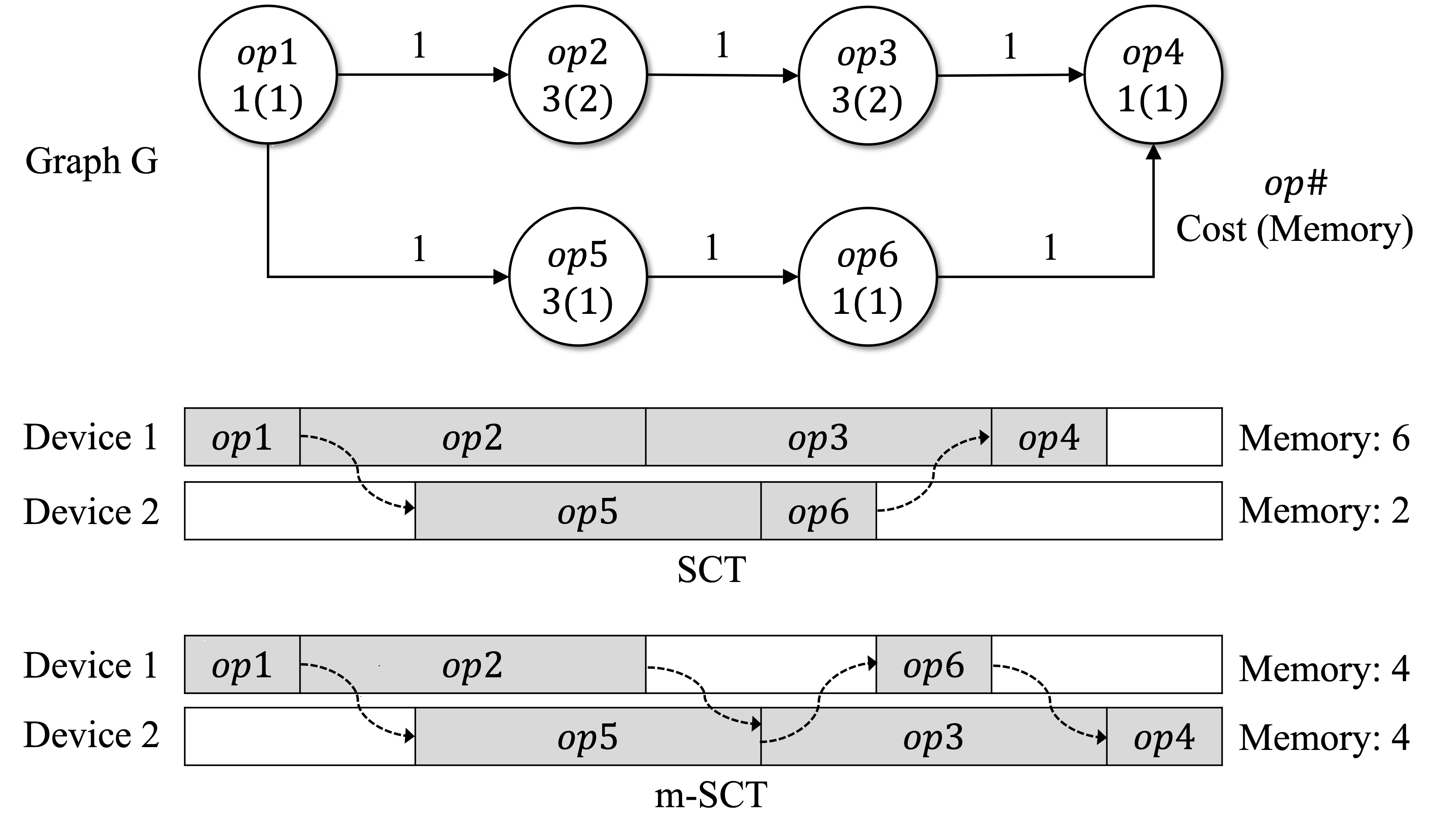
Figure 1. Classical SCT vs. m-SCT. When per-device memory is limited to 4 memory units, SCT OOMs but m-SCT succeeds. m-SCT’s training time (makespan) is only slightly higher (9) than SCT with infinite memory (8). Dashed arrows show data transfers.

Optimality of m-ETF and m-SCT

Classical ETF and SCT were originally proposed to schedule a DAG of tasks on $n$ processors. The original work (Hanen and Munier, 1995; Hwang et al., 1989) derived upper bounds on the makespan achieved by them. Processor memory was not considered in that original formulation, and infinite memory was assumed.

On the contrary, in ML model training, each device has a memory constraint. Impact of memory on scheduling is further pronounced due to the persistent memory that each task requires. Consequently, the schedules obtained by m-SCT/m-ETF can differ significantly from the SCT/ETF schedules (i.e., without memory constraint)—Fig. 1 shows an example. It is not clear how much worse m-SCT/m-ETF makespan is, compared to the optimal. Thus we derive upper bound on makespan of both m-ETF and m-SCT by extending the proofs in (Hwang et al., 1989) and (Hanen and Munier, 1995) to the memory constrained case. We show that m-SCT/m-ETF makespans are within a constant factor of the optimal makespan.

Because the proofs for optimality of m-ETF and m-SCT are involved, we show them in Appendix A and Appendix B respectively. We summarize our results and approach here:
Result 1: The completion time of m-ETF under realistic communication cost and limited memory, is within a known factor of the optimal schedule possible under zero communication cost but with infinite memory.
Result 2: The completion time of m-SCT under realistic communication cost and limited memory, is within a known factor of the optimal schedule under infinite memory.
Intuitively, our derived upper bounds are proportional to the ratio $\frac{n}{r}$,where $n$ is the total number of devices available, and $r$ is the number of devices out of $n$ that still have spare memory after all the tasks have been placed in a way that “fills up” memory device by device. Note that $\frac{n}{r}>1$, otherwise the problem is unsolvable. Intuitively, a smaller $\frac{n}{r}$ (i.e., larger $r$) indicates looser memory constraint and thus better makespan. As $\frac{n}{r}$ approaches 1, m-SCT’s solution (respectively m-ETF’s) starts to approach that of SCT (respectively ETF).

Baechi Design

This section describes how we implement Baechi in a way that works modularly with TensorFlow (Abadi et al., 2016) as well as PyTorch (Paszke et al., 2019), two popular open-source learning platforms originally developed by Alphabet and Meta respectively.

At a high level—for both target systems, Baechi first creates a computation graph of the input model, where each node is annotated with its memory requirements and time to complete. This graph is then fed to the chosen algorithm (Section 2’s m-SCT, m-ETF, or m-TOPO) to generate the placement. Finally, training is automatically executed with the given placement and without requiring the developer to modify the code for the model.

However, because of two key differences in abstractions and architectures between TensorFlow and PyTorch, Baechi’s design for each is slightly different. First, the “nodes” in the computation graph are operators in TensorFlow while in PyTorch they are modules. The former are fine-grained mathematical operations on tensors, while the latter are coarser structures similar to classes in object-oriented languages. Second, in TensorFlow a model is a static graph of operators, while in PyTorch, the computation graph is constructed only during the forward run. Because of foreknowledge of the graph, TensorFlow can automatically insert rendezvous operators (Tensorflow, 2022) for cross-device communication. However, PyTorch does not automatically insert these essential cross-device communication primitives. It requires PyTorch developers to write explicit code that moves tensors across devices during execution. A side benefit of our work is the automatic generation of these communication primitives.

In the remainder of this paper, we refer to the integration of Baechi into TensorFlow as Baechi-TF, and Baechi’s integration into PyTorch as Baechi-PY.

Next, we describe our techniques and optimizations for Baechi-TF in Section 3.1, and then additional changes and differences required for Baechi-PY design in Section 3.2.

Design of Baechi-TF

To work with TensorFlow, Baechi needs to address four challenges:

1) Satisfying TensorFlow’s colocation constraints, 2) Minimizing Data Transfer via Co-Placement, 3) Optimizations to reduce the number of operators to be placed, and 4) Accommodating Sequential and Parallel Communications. Baechi solves these using a mix of both new ideas (Sections 3.1.1,3.1.3,3.1.4) and ideas similar to past work (Sections 3.1.2,3.1.3).

Working Example. We use Figure 3 as a working example throughout this section. It is a simplified TensorFlow graph for linear regression training with stochastic gradient descent (SGD).

TensorFlow Colocation Constraints

The first challenge arises from the fact that TensorFlow (TF) requires certain operators to be colocated. For instance, TensorFlow offers a variable operator, tf.Variable, which is used to store persistent state such as an ML model parameter. The assignment and read operators of a variable are implemented as separate operators in TensorFlow, but need to be placed on the same device as the variable operator. TensorFlow represents this placement requirement as a colocation group involving all these operators. E.g., in Figure 3 there are two colocation groups: one containing Weight and ApplyGrad, and another containing Step and UpdateStep.

Baechi’s initial placement (using the algorithms of Section 2) ignores colocation requirements. Our first attempt was to post-adjust placement, i.e., to “adjust” the device placement, which was generated ignoring colocation, by “moving” operators from one device to another, in order to satisfy TF’s colocation constraints. We explored multiple post-adjustment approaches including: i) preferring the device on which the compute-dominant operator in the group is placed, ii) preferring the device on which the memory-dominant operator in the group is placed, and iii) preferring the device on which a majority of operators in the group are placed. We found all these three approaches produced inconsistent performance gains, some giving step times up to 406% worse than the expert. We concluded that post-adjusting was not a feasible design pathway.

Baechi’s novel contribution is to co-adjust placement, using colocation constraint-based grouping while creating the schedule. (In comparison, e.g., ColocRL (Mirhoseini et al., 2017) groups before placement.) Concretely, whenever Baechi places the first operator from a given colocation group, all other operators in that group are immediately placed on that same device. Baechi tracks the available memory on each device given its assigned operators. If the device cannot hold the entire colocation group, then Baechi moves to the algorithm’s next device choice. We found this approach the most effective in practice, and it is thus the default setting in Baechi.

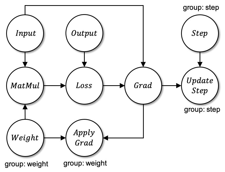
Figure 2. Working Example. ML Graph for Linear Regression.

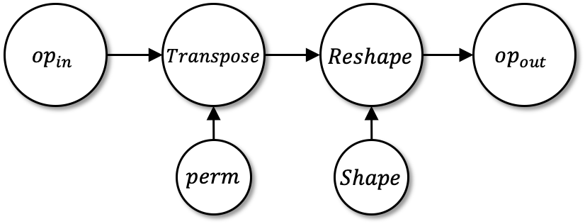
Figure 3. Co-Placement. Subgraph of tf.tensordot Generating Data Transfers by m-ETF.

Co-Placement Optimization

Different from TensorFlow’s colocation constraints (Section 3.1.1), Baechi further prefers to do co-placement of certain operators. This is aimed at minimizing data transfer overheads. Common instances include: (i) groups of communicating operators whose computation times are much shorter than their communication times, and (ii) matched forward and backward (gradient-calculating) operators.

Figure 3 shows an example for case (i). This subgraph generated by tf.tensordot API is a frequent pattern occurring inside TensorFlow graphs. The subgraph permutes the dimensions of $\texttt{op}_{\texttt{in}}$ output according to the perm’s output (Transpose) and then changes the tensor shape by Shape’s output (Reshape).

When m-ETF places this subgraph on a cluster of 3 devices, it places $\texttt{op}_{\texttt{in}}$, perm, and Shape on different devices. Computation costs for perm and Shape are very short (because they process predefined values), whereas subsequent communication times are much larger. Thus, m-ETF’s initial placement results in a high execution time.

Baechi’s co-placement heuristic works as follows. If the output of an operator is only used by its next operator, we place both operators on the same device. This is akin to similar heuristics used in ColocRL (Mirhoseini et al., 2017). In Figure 3,

Baechi’s co-placement optimization places all of the operators on one device, avoiding any data transfers among the operators.

For case (ii), to calculate gradients in the ML model, TensorFlow generates a backward operator for each forward operator. Baechi co-places each backward operator on the same device as its respectively-matched forward operator.

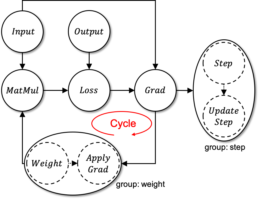
(a)

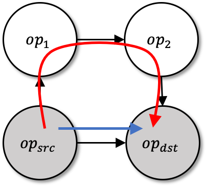
(b)

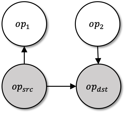
(c)

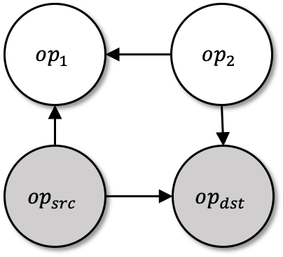
(d)

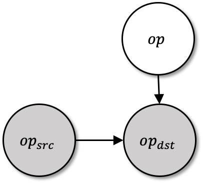
(e)

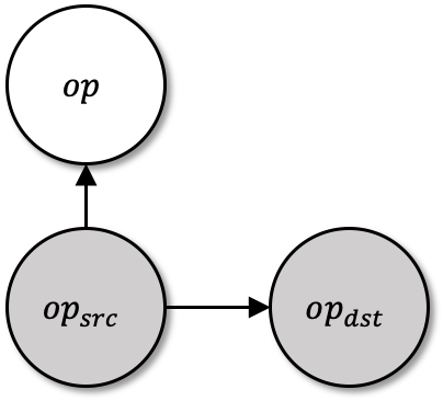
(f)

Figure 4. Operator Fusion Without Creating Cycles. (a) shows a fused ML Graph Example. When $op_{src}$ and $op_{dst}$ are fused, some scenarios create a cycle (b), while others do not (c, d, e, f). Baechi fuses operators in a subset of “safe” cases, particularly (e, f).

Upon placing the first operator in a colocation group, Baechi uses both the co-placement heuristic and the colocation constraints (Section 3.1.1) to determine which other operators to also place on the same device. Co-placement not only minimizes communication overheads but also speeds up the placement time by reducing the overhead of calculating schedulable times on devices.

Operator Count Minimization

Placement time can be decreased by reducing the number of operators/groups to be placed. We do this via two additional methods:
i) Operator Fusion: Fusing operators that are directly connected and in the same co-placement group; and
ii) Forward-Operator-Based Placement: Placing operators by only considering the forward operators.

Operator Fusion. Baechi fuses operators using either the colocation constraints (Section 3.1.1) or co-placement optimizations (Section 3.1.2). This is new and different from TensorFlow’s fusion of operations. One challenge that appears here is that this may introduce cycles in the graph, violating the DAG required by our algorithms.

Figure 4(a) shows an example resulting from Figure 3—a cycle is created when Step and UpdateStep are fused into a new meta-operator, and Weight and ApplyGrad are fused.

Consider two nodes–source and destination–with an edge from source to destination. Merging source and destination creates a cycle if and only if there is at least one additional path from source to destination, other than the direct edge. Note that there cannot be a reverse destination to source path as this means the original graph would have had a cycle.

In Figure 4(b), fusing $\texttt{op}_{\texttt{src}}$ and $\texttt{op}_{\texttt{dst}}$ creates a cycle. Unfortunately, we found that pre-checking existence of such additional paths before fusing two operators is unscalable, because the model graph is massive.

Instead, Baechi realizes that a necessary condition for an additional path to exist is that the source has an out-degree at least 2 and the destination has an in-degree at least 2 (otherwise there wouldn’t be additional paths). Thus Baechi uses a conservative approach wherein it fuses two operators only if the negation is true, i.e., either the source has an out-degree of at most 1, or the destination has an in-degree of at most 1 (Figures 4(e), 4(f)). This fusion rule misses a few fusions (Figures 4(c), 4(d)) but it catches common patterns we observed, like Figure 4(e).

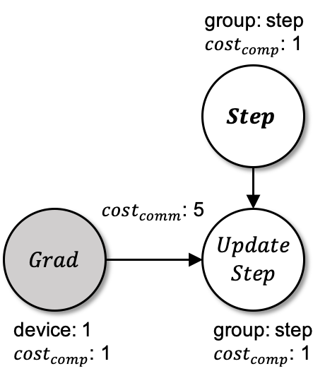
(a)

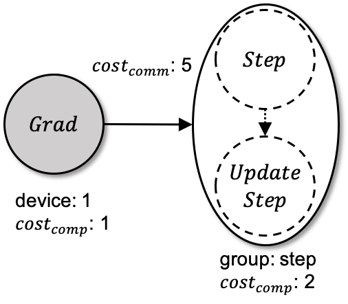
(b)

Figure 5. Operator Fusion. Avoiding Data Transfer Example. (a) Before Fusion. (b) After Fusion.

Forward-Operator-Based Placement. When memory is sufficient (i.e., one device could run the entire model), Baechi considers only forward operators for placement and thereafter co-places each corresponding backward (gradient) operators on the same respective device as their forward counterparts. This is a commonly-used technique (Mirhoseini et al., 2017; Addanki et al., 2019). This significantly cuts placement time. When device memory is insufficient, Baechi runs the placement algorithms using both forward and backward operators, forcing corresponding pairs to be co-placed using the heuristic of Section 3.1.2.

Example: Benefits of Fusion. Figure 5(a) shows the placement of a subgraph of Figure 3 on two devices. Baechi first places Grad on device-1. Baechi places the next operator, Step on the idle device-2, and colocates (due to TF constraints) UpdateStep on device-2. This creates communication between the devices. Assuming operators’ compute costs are 1, and communication cost between Grad and UpdateStep is 5, this results in an execution time of 7 time units.

On the other hand, Figure 5(b) shows that Baechi merges Step and UpdateStep with operator fusion. Since this meta-operator’s schedulable time on device-1 is earlier than on device-2 due to communication overhead, Baechi places it on device-1. Fusion lowers total execution time to 3 time units.

Loops in the Original Model Graph. Different from the cycles discussed above, some network graphs consist of loops, e.g., RNNs. We use the unrolled ML graph (Allen and Cocke, 1972) to turn the graph into a DAG, and then apply Baechi’s techniques.

Sequential vs. Parallel Communication

Our algorithms from Sections 2.3 and 2.4 assume that each operator can send data simultaneously to its children. Baechi also proposes a new way to deal with environments involving constrained networks (including our deployment in Section 5), where data transfer is sequential. For networks that limit each device to do at most one transfer at a time (out or in), Baechi assumes communication queues at devices. Concretely, when a data transfer between two devices is requested, Baechi assumes the request is put into the respective devices’ communication queues and processed sequentially at both ends. During placement, Baechi calculates the wait time at the communication queues and adds it to the earliest schedulable time computed for the operator. Specifically the queue wait time is added to equation (1) in Section 2.3. Otherwise, normal m-SCT/m-ETF apply, as described earlier.

Design of Baechi-PY

We remind the reader that unlike TensorFlow’s fine-grained operators and known communication graph, PyTorch: (i) has coarser modules, and (ii) requires the programmer to explicitly program cross-device communication.

Concretely—first, PyTorch models are built by composing different modules. The model is not natively available as a graph unlike TensorFlow. To feed the model to Baechi’s algorithms, Section 3.2.1 describes how we construct a graph by using PyTorch’s Autograd (Paszke et al., 2019) which tracks the flow of tensors among the modules of the model. Second, the primitive .to() API provided by PyTorch for developers to program communication is inefficient and manual. To address this, Section 3.2.2 presents our communication protocol to handle cross-device transfers efficiently and automatically.

Baechi-PyTorch Graph

Developers build PyTorch models by composing modules, i.e, classes inherited from PyTorch’s nn.Module. Each module contains its tensor parameters (e.g., weights of a linear layer) and a forward() method, which defines how the module modifies the input. By default Baechi treats modules as the nodes of the graph in Baechi-PY. Placing a module on a device means moving all its parameters to the device before beginning the training. During the training, our communication protocol (next Section 3.2.2) ensures that the input to that module is also moved to the same device. Subsequently the forward() operation of the module will be invoked at runtime, and it will be executed on the assigned device. A model may also include operations not defined as PyTorch modules. For instance, arithmetic operations like scaling (e.g: x=x/2). But these operations usually do not have any associated parameters that must be assigned to a device by Baechi-PY. Hence we exclude them from the graph during the placement planning. By default, this associated operation will be executed on the device of the input tensor, i.e., x’s device in this case.

Baechi-PY constructs the model’s graph in two steps. First we obtain all modules that constitute the model and co-place modules occurring in common design patterns. Second we obtain the edges of the graph by tracking the flow of tensors using PyTorch’s Autograd (Paszke et al., 2019). This approach is similar to PipeDream (Harlap et al., 2018).

Co-placement: Treating modules as nodes, we observed it is common for models to contain specific subgraphs (of modules) that occur as common design patterns throughout the model graph. Baechi-PY groups such subgraphs into a single node—this is called co-placement (unlike Baechi-TF’s co-location constraints in Section 3.1, this co-placement is a performance optimization in PyTorch). For instance in Inception models, the subgraph (Conv2d)$\rightarrow$ (Batch Norm) $\rightarrow$ (inplace ReLU) occurs commonly, and Baechi-PY groups each occurrence as one node in the computation graph. This co-placement allows Baechi-PY to avoid communication of tensors along the two edges of this subgraph. An additional benefit of co-placement is that it significantly reduces the size of the computation graph, thus making Baechi’s algorithms (Section 2) run faster. For instance, co-placement reduces the number of nodes in Inception-V3 PyTorch by 60%, from 325 to 133. By default, Baechi-PY uses the most atomic modules, i.e., not further divisible, e.g., 2D Convolution module (Conv2d). If the developer wishes, they can programmatically specify which modules Baechi-PY should be co-placed and treated as individual nodes.

Building the graph: Next, Baechi obtains edges between the nodes. To do this, we run a training step of the model with dummy data. (We run 20 such dummy training steps, also helping us profile memory usage and computation times of all the nodes.) During the forward run, we annotate each intermediate output tensor with the node that generated it. Meanwhile, PyTorch’s Autograd automatically fills in the gradient function (grad_fn) for each tensor created. Further, each such grad_fn has a list of grad_fn of tensors used as inputs in creating this tensor. Autograd stores this list to perform back-propagation later. We use this information that traces the tensor gradient functions, along with our tensor to node annotation, to construct a dependency graph among modules of the model.

It is possible that some gradient functions may include operations not related to any module, e.g., Autograd-specific operations such as SelectBackward or gradients of arithmetic operations. But since these operations do not need a device placement, they are removed to obtain the dependency graph only between nodes of the model (they are added back in after the model is placed) .

Communication Protocol

PyTorch provides native support for synchronous communication, which can be inefficient. If asynchronous data transfer is used, the developer is required to carefully insert synchronizations to ensure correctness.

We design a general communication protocol for cross-device communication that is efficient and automated, thus relieving the developer from specifying manual configurations. We do so by leveraging CUDA streams, an abstraction that allows overlapping multiple sequences of operations in a GPU (Nvidia, 2022).

To move a tensor T to $GPU_{0}$, PyTorch provides an API T.to(0). To ensure correctness, .to() conservatively blocks both sending and receiving devices until all the operations submitted to both devices so far are completed. This can be avoided by leveraging the abstraction of CUDA streams (Nvidia, 2022), in order to overlap communication with computation. A CUDA stream in a GPU is a FIFO queue of operations that will be sequentially executed on the GPU. By default, all operations submitted to a GPU are placed on a single stream. To perform two operations in parallel, they must be placed on two separate streams on the GPU. Accordingly, on each GPU, Baechi-PY defines one compute stream and multiple communication streams. The compute stream queues the computations corresponding to the modules placed on the GPU, while the communication streams concurrently move the relevant tensors across the devices.

However, CUDA streams need to be programmed carefully to specify synchronization points that obey dependencies in the model graph. We use CUDA Events provided by the runtime API (PyTorch, 2022a) to synchronize the independent streams.

None of the existing ways of using CUDA streams in PyTorch fits our needs. Concretely—first, in PyTorch-Distributed (Li et al., 2020) and PipeDream (Harlap et al., 2018), training steps proceed in stages, each working on a different batch of data. All tensors generated in a given stage are transferred to the next device at the end of the stage. This pattern, where all communication happens synchronously only after all computations are complete requires few, if any, synchronizations. In contrast, Nimble (Kwon et al., 2020), deals with multiple parallel streams working on the same batch of data, like in Model Parallelism. Compute and communication events may asynchronously occur at any time and it requires synchronizations to preserve data dependencies. However, Nimble is a single-GPU system.

In Baechi-PY, we use a greedy-wait strategy. Concretely, first we greedily push out the output of a node, as soon as it is computed, to the devices of its children nodes. Second, before starting the compute operation, a child node must wait for all its incoming input stream or if the input has already been transferred it must pull the copy of the inputs on its devices. We implement our greedy-wait communication protocol as a wrapper around the forward() function of each node.

1

2

3for each parent of the node in graph do

4      (node’s compute_stream) wait for (rx_stream from parent’s device);

5     

6      end for

7     On node’s compute_stream:

8        input_local = local copies of input on node’s device;

9        output = forward_operation(input_local);

10      for each child of the node in graph do

11           (tx_stream to child’s device) wait for (node_compute_stream);

12          

13           end for

14          for each child of the node in graph do

15                Using (node’s tx-rx_stream pair to child’s device ):

16                  send output to child;

17               

18                end for

return output

Algorithm 1 Communication protocol built around each node’s forward(input)

Algorithm 1 shows the complete communication protocol, and we describe it in detail. Before we start the training, for a given node and its child node on a different device, we create two streams - a tx-stream on the node’s device and a rx-stream on the child node’s device. Only one such stream pair is sufficient for a child device, even if multiple children nodes are on that device. So if a node on $GPU_{0}$ has two children, one on $GPU_{1}$ and another on $GPU_{2}$, then for that node we create one tx-rx stream pair each to $GPU_{1}$ and $GPU_{2}$. We do this for every node and for every device any of its child nodes reside in.

Each device’s compute stream queues the computations of nodes assigned to that device. When a node reaches the head of the compute stream of its device, the compute stream is made to wait for all the rx-streams to that device from all the parent nodes (line 2). The rx-streams carry a copy of the output tensors of the parent nodes to the device of the current node. Once all rx-streams have completed the transfer, these tensors are passed as inputs to the actual forward computation of the node (lines 4-6). All the tx-streams egressing from this node are made to wait for the compute stream to finish the computation (lines 7-9). The tx-stream carries the outputs of the node to the child node’s device and the corresponding rx-stream on the child node’s device receives it. As soon as the output is ready, it is asynchronously sent to all the child devices through the tx-streams and received asynchronously at the child devices through their respective rx-streams (lines 10-12). The compute stream can move to the next node assigned to it while the tx-streams are transferring out the output. Similarly, the compute streams on child devices are not interrupted by incoming tensors on their rx-streams. Note that the output is sent to a child device only once even if multiple children reside on that child device. The tx-rx streams serve as synchronization points in addition to overlapping communication and computation.

Our m-ETF and m-SCT algorithms from Sections 2.3 and 2.4 assume that each node can send data simultaneously to its children. Our protocol mimics this communication with multiple outgoing tx-streams transferring the tensors to child devices in parallel. While such overlapping tx-streams from a device may slightly increase the communication times in each of the streams, we observed that the associated effect on step time is small. Also as long as we facilitate and synchronize the forward run correctly, PyTorch’s Autograd (Paszke et al., 2019) ensures that the back-propagation correctly executes in the reverse order of the forward sequence. It automatically manages input-output dependencies and synchronizations in the reversed order.

Implementation

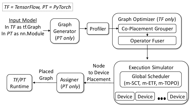
Figure 6. Baechi System Architecture

In order to integrate modularly with TensorFlow (TF) (Abadi et al., 2016) v1.12 and PyTorch v1.9 (Paszke et al., 2019), Baechi adopts the architecture shown in Figure 6. Baechi executes the following steps: 1) its Graph Generator and Profiler constructs the graph annotated with each node’s time and memory requirements, 2) Baechi’s Graph Optimizer for TensorFlow uses the design of Section 3.1 to account for TF colocation constraints, and applies co-placement and operator fusion, 3) Baechi’s Execution Simulator (ES) (Section 4.2) executes our algorithms (m-TOPO, m-ETF, or m-SCT) and generates the placement (in TensorFlow a ready-to-use placed graph is output), and 4) the Assigner for PyTorch (Section 4.3) modifies the model to allow execution according to the generated placement. The placed graph can then be used in the training script as the drop-in replacement for the single-GPU model, in both TensorFlow and PyTorch. Next we describe each of the components in detail.

Graph Generator, Profiler and Optimizer

In Baechi-TF, the model is already given as a static graph. The Profiler then measures and annotates each node with its time and memory requirements. Baechi parses this annotated graph and generates an equivalent intermediate NetworkX (Schult, 2008) graph. The NetworkX format allows Baechi to both store operator execution metadata (computation and communication times, memory needed, etc.), and to easily manipulate the graph (e.g., fuse operators). Then, in case of Baechi-TF, we additionally apply the co-placement and operator fusion optimizations (Sections 3.1.2, 3.1.3) to the graph.

In Baechi-PY, the Graph Generator constructs the graph corresponding to the input model as per Section 3.2.1.

For communication time, we use a linear model proportional to data size. Concretely, we implemented a microbenchmark tool to measure communication times for various data sizes, and generated a communication cost function through linear regression.

Profiler:

The Profiler measures computation times and memory requirements of each node in the graph. In Baechi-TF, we use the standard TensorFlow profiling tool to obtain computation time and memory allocation for each operator. TensorFlow profiler returns allocation information for temporary, permanent, and output tensor memory. The temporary memory is allocated at the beginning of an operation and deallocated when the operation finishes. The permanent memory is allocated and used over the entire execution, e.g., to store persistent states such as weights. For Baechi-PY we build a simple profiler, akin to that in (Harlap et al., 2018), for measuring time using hooks (PyTorch, 2022b), and for measuring memory .

Baechi-PY Profiler Memory Estimation

In PyTorch, GPU Memory required to hold all the tensors is reserved once during the first training step and reused in subsequent steps. To model the memory usage pattern, we categorize each node’s memory as consisting of 5 components:

1. Parameters memory: Memory occupied by parameters of the node;

2. Output Memory: forward output of the node;

3. Parameter gradient: gradients of parameters of the node;

4. Upstream gradient: gradient of output of the node;

5. Memory temporarily used in computing the output/gradient.

Memory	Inference	Training
Permanent	(a)	(a) + (b) + (c)
Temporary	(b) + (e)	(e) + (d)

Table 2. Memory Consumption in PyTorch

Table 2 summarizes how these five metrics are used in training and inference, and whether they are used as temporary memory or permanent memory. We describe each term. During the training phase, each node requires memory to store: (a) its parameters, (b) the node’s forward output tensors, and (c) parameters’ gradient information. In PyTorch, memory to store parameter gradient information is acquired once in the beginning of training and permanently held until the end of training. Similarly, output tensors ((b)) are treated as permanent memory since during each forward run, outputs of all nodes must be stored. They are required later during back-propagation. In contrast during the inference phase (forward only runs), output of a node is temporary since it is immediately released after being consumed by the subsequent node. During back-propagation in training, memory is also required to hold the gradient of output of the node ((d)). This is a temporary requirement since this memory is released after the output gradient has been used to compute the node’s parameter gradients and its input gradient. Nodes may also require temporary memory while performing these computations ((e)). For example, in computing the parameter gradients, a temporary matrix is used to store all the gradients and then the node’s parameter gradients are updated at once. For in-place nodes like the in-place ReLU, (b) is set to 0 since no new output tensor is generated ((a) and (c) are also 0 incase of ReLU since it has no associated parameters).

Execution Simulator

Baechi’s Execution Simulator (ES) executes the algorithms on the profiled graph and generates the placement. The ES takes as input the NetworkX operator graph, the number of GPUs and the memory capacity of each of them. The output is the graph in which all operators are assigned to devices. We describe the common parts of the ES across both Baechi-TF and Baechi-PY, explicitly pointing out differences as necessary.

Our initial attempt was in fact to try re-purposing TensorFlow ’s (existing) simulator, but using that required us to assume operators were already placed, zero communication cost, and no caching—these were inapplicable to Baechi. Motivated by this, we designed Baechi’s new ES uniquely for memory-constrained placement.

The ES consists of: a) a global scheduler, and b) simulated devices (with specs identical to deployment). The global scheduler maintains a single queue with operators that are ready to run. The scheduler extracts operators from its queue and applies our scheduling algorithms (m-TOPO, m-ETF, m-SCT) to place them on devices.

In ES, each device has two FIFO queues, one for operators and one for data transfer. This allows data transfer to overlap with operator execution. When a device receives a tensor from another device, it caches the tensor to avoid duplicate data transfer.

Dynamic Memory Allocation.

Calculating a device’s memory usage as the sum total of all its assigned operators (assigned over the entire duration) clearly overestimates memory. For example in TensorFlow, Inception-V3 with batch size 32 can execute using 4 GB even though its operators’ memory needs add up to 22 GB.

In generating the placements, the ES calculates memory in a way that parallels how the frameworks manage memory. Concretely Baechi’s ES tracks an estimate of memory usage during its placement. When an operator executes on a device, the device allocates temporary memory, and separate memory for its output tensors. The temporary memory is deallocated when the operator finishes. There are minor differences in the ES for TensorFlow and PyTorch. TensorFlow uses separate operators for forward and backward computation. The output memory of an operator is deallocated after all its successors finish. In PyTorch, the forward and backward computation runs in a single module. The output memory of a module is held until its backward computation is completed. The output memory is treated as a part of the permanent memory as explained in the previous Section 4.1. If a device’s memory becomes full, the device can be removed–this never happens in practice as usually a device has at least a few bytes left.

Note that in Baechi-TF, memory is reserved for a colocation group at device $p$ when the first operator is placed on $p$ (Section 3.1.1). The reserved memory is deallocated when all the operators in the group finish.

Linear Programming Solver. To solve the SCT LP problem, we use the interior point method (Boyd and Vandenberghe, 2004). This is preferable over other solvers such as simplex (Bartels and Golub, 1969) as it guarantees polynomial execution time (Tomlin, 1989). Concretely, we use the primal dual interior-point solver via Mosek optimization (Andersen and Andersen, 2000), which has a run time complexity of $O(n^{3.5}L)$, where $L$ is the maximum number of bits in the LP input, and $n$ is the number of variables.

Assigner in Baechi-PY

Once the mapping of graph nodes to devices is decided, the Assigner contains the mechanism to initialize the assignment. The Assigner for TensorFlow merely changes the device attribute of the nodes. The Assigner for PyTorch requires multiple steps—it needs to: i) move nodes’ parameters to the assigned devices, ii) send output tensors from a node to devices of child nodes at the device boundaries, and iii) avoid naive use of .to() for cross-device communication as this leads to inflated step times owing to unnecessary blocking of the devices (see Section 3.2.2).

Baechi-PY’s Assigner enables this process by automatically adding wrappers around the forward() methods of the nodes. The wrapper transparently handles the communication and caching of the tensors using the communication protocol in Section 3.2.2. This way, the developer does not need to make any changes to the input model code written for a single-GPU execution. The output of the Assigner is a model assignment that can be used as a drop-in in any existing training script.

Miscellaneous Issues

We discuss a few key miscellaneous aspects.

LP Modifications. The ILP solutions (Section 2.4) resulted in more than one favorite child (or parent) being selected for certain nodes. In Baechi we lowered the rounding threshold from 0.5 to below 0.2. This eliminated all violations, and avoided nodes from having multiple favorite children. (We use threshold = 0.1 in practice.)

Ignoring Bootstrap Steps in Profiling. 1) In a training run of a model graph, step times are initially high due to TensorFlow bootstrapping. We estimate step times in steady state, after a few iterations have passed. 2) Some TensorFlow operators are implemented with multiple GPU kernels. When profiling these operators, we include multiple kernel executions, in order to avoid underestimation. This is similar to TensorFlow’s cost model (Abadi et al., 2016).

Reordering Layers in PyTorch. Dynamic line-by-line execution in PyTorch means that the modules’ forward() functions will be called in the order in which they appear in the code rather than in the topological order followed by Baechi’ ES (Sec. 4.2). We reorder the actual execution of modules’ computations on GPUs by launching a thread when a module’s forward() is called. The thread waits until its topological parent (according to the ES) has submitted the computation task to the GPU and only then submits its task. However, such reordering does not give a noticeable advantage over just executing the code order since the two orders do not differ significantly in most cases.

Evaluation

Our evaluation answers the following six questions:
1. How fast is Baechi’s placement time, i.e., how quickly do our algorithms find placements? (Section 5.2)
2. How fast are the step times of the placement generated by Baechi, i.e., training time per step of the placed model? (Section 5.3)
3. How do the step times for Baechi compare to single GPU and expert placements? (Section 5.3)
4. How do the Baechi’s step times change when there is insufficient memory per GPU? (Section 5.4)
5. How much is the benefit due to Baechi’s optimizations from Sections 3.1.2, 3.1.3 and 3.2.2? (Section 5.5)
6. Are algorithmic approaches preferable over RL approaches for model parallelism? (all subsections).

Experimental Settings

We use two popular ML benchmarks for each framework: A) for TensorFlow, we use Inception-V3 and Google Neural Machine Translation System (GNMT), and B) for PyTorch, we use Inception-V3 and a Transformer model. The former choice is because: i) Inception-V3 and GNMT are respectively considered the best representatives of vision and Natural Language Processing (NLP) models, and ii) past work (Addanki et al., 2019; Mirhoseini et al., 2017, 2018) used Inception-V3 and NMT (GNMT is a more complex version), thus allowing us to compare. For PyTorch we replace GNMT with Transformer as the former is implemented using the LSTM module (PyTorch, 2022c), making the (latter) Transformer a more complex and generalized version. We describe the three benchmark configurations in detail below:

Inception-V3 Benchmark Configuration. Inception-V3 (Szegedy et al., 2016) is a convolutional neural network architecture that is widely used for image classification. This model is composed of multiple blocks called Inception modules. The Inception modules consist of branches of convolutional and pooling operators. To train the model, we use RMSProp (Hinton et al., 2012) and batch sizes of both 32 and 64.

GNMT Benchmark Configuration. Google Neural Machine Translation System (GNMT) (Wu et al., 2016) is a language model for automated translation. GNMT consists of: encoder and decoder modules, each a stack of recurrent neural networks (RNNs); and the attention module to process long sequences effectively. We use 4 long short-term memory (LSTM) layers of the encoder and the decoder layers with residual connections, and the Bahdanau attention mechanism (Bahdanau et al., 2015). We use the LSTM hidden size of 512, the vocabulary size of 30,000, the unrolled RNNs with the sequence length of 40 and 50, and the batch size of 128 and 256. Baechi-TF applies the co-placement optimization to LSTM cell operators and also to attention operators.

Compared to Inception-V3, GNMT has fewer barriers (sync points) inside its model graph, indicating that GNMT has a higher potential to benefit from Baechi-TF’s parallel placements.

Transformer Benchmark Configuration. Transformers are a versatile family of models used in vision as well as language. Like Neural Machine Translation (NMT), Transformers have an encoder-attention-decoder architecture. But while NMT processes one word at a time, Transformers use multi-head attention modules that process the entire sequence at once. In PyTorch, we implement an attention operation in the traditional way (GitHub, 2022)—as one large matrix multiplication and hence as a single module. For concreteness, we use the base Transformer model from (Vaswani et al., 2017) (without weight sharing) with a vocabulary size of 30,000, sequence length of 50 and batch sizes of 64, and 128.

Machine Setup. All experiments are run on our local server that has 4 NVIDIA GTX 2080 GPUs, with 8 GB per-GPU memory (the machine also has an Intel i9-7960X CPU, but this is not used to execute operators). GPUs are connected to CPUs via PCIe 3.0 x16 (we do not use NVLink (NVIDIA, 2022)). All data transfers go through the host memory (no P2P communication among GPUs). This results in a slow IO bus, and we believe this high ratio of communication overhead to computation overhead is representative of realistic scenarios like the kinds outlined in Section 1. We place all GPU-supported operators only on GPUs.

Approach to Comparison. To quantify the benefits of using an algorithmic approach to model parallelism over a Reinforcement Learning (RL) approach for model parallelism, we compare Baechi to the best RL-based model parallelism techniques: (Addanki et al., 2019; Mirhoseini et al., 2017, 2018). Directly running these other systems was complicated by lack of uniform availability of working code—Placeto’s code (Addanki et al., 2019) missed key optimizations; ColocRL (Mirhoseini et al., 2017) is proprietary; only HierarchicalRL’s code (Mirhoseini et al., 2018) was available, but it was slow and generated inefficient placements. E.g., For GNMT, HierarchicalRL took 12 hours+ to run placement (batch size 128, length 50) and the resultant step time was much higher than expert’s, contrary to HierarchicalRL paper’s claims. Essentially, direct comparison would be unfair to these other papers without knowing the exact hyperparameters they used to achieve their “best” performance. In light of this, our comparison gives the benefit of doubt to, and uses the best performance from, these learning-based placement papers. All the above papers compared step times to experts, and we do too. We do not compare to other algorithmic techniques for model parallelism (listed in Section 1) because of either: their standalone nature (Tarnawski et al., 2020) (making a TensorFlow/PyTorch comparison unfair), or their limitation to Transformers (Li et al., 2021; Shoeybi et al., 2019), or because they are already shown to be comparable to our performance (Hafeez et al., 2021). This also keeps our evaluation focused on comparing algorithmic approaches to RL approaches for model parallelism.

Model	HierarchicalRL (Mirhoseini et al., 2018)	Placeto (Addanki et al., 2019)	Baechi (m-SCT)
Inception-V3	11 hrs 50 mins	1 hr 49 mins	1-10 seconds
NMT (GNMT)	1 day 21 hrs 14 mins	2 days 20 hrs 40 mins	1.2-48 seconds
Transformer	N/A	N/A	1-3 seconds

Table 3. Placement Time. Time to Generate a Placement for our target machine with 4 GPUs.

Placement Time

Table 3 shows both: 1) measured placement times of Baechi, and 2) calculated placement times for two learning-based techniques, namely: HierarchicalRL (Mirhoseini et al., 2018) and Placeto (Addanki et al., 2019). The numbers for HierarchicalRL and Placeto are normalized quantities, both derived from numbers reported in Addanki et al. (Addanki et al., 2019). For these two systems, we multiply the fastest step time among its reported placements, by the number of placement samples. For instance, HierarchicalRL’s (Mirhoseini et al., 2018) Inception-V3 placement training time is derived as a product of the reported final step time (1.19 s) and the number of samples (35,800), giving 42,602 s, or 11 hrs 50 mins.

Hence, the numbers for these learning-based placers are their best-case performance. In comparison, we use the worst-case placement times from Baechi, specifically from m-SCT which took the longest to generate a placement. Note that all times in Table 3 exclude time to profile the graph, as profiling is a common baseline encountered by all the three approaches shown. We find the profiling time to be low: about 10–12 s total for Inception-V3 and GNMT in Baechi-TF, and about 11–14 s for Inception-V3 and Transformer in Baechi-PY. For instance, in Baechi-TF, this breaks down as 2-4 s for warmup execution, 1–3 s for graph execution for profiles, and less an 1 s for parsing profile results.

Table 3 shows that Baechi places ML models orders of magnitude faster than the learning-based approaches. For Inception-V3, Baechi reduces placement time, from 1.8–11.8 hours (using existing techniques (Mirhoseini et al., 2018; Addanki et al., 2019)), to under 10 s in both Baechi-TF and Baechi-PY. Thus Baechi is $654\times$–$42.6$K$\times$ faster at placing Inception-V3. For GNMT, Baechi-TF reduces placement time from several days to under 48 s. Thus Baechi is $3392\times$–$206$K$\times$ faster at placing GNMT. For Transformer, Baechi-PY places it under 3 s. Because HierarchicalRL and Placeto (Addanki et al., 2019; Mirhoseini et al., 2018) did not include Transformers in their evaluation, the corresponding entries are marked as not available in Table 3.

Overall, Baechi is $654\times$–$206$K$\times$ faster at placement compared to today’s learning-based approaches (Addanki et al., 2019; Mirhoseini et al., 2018).

Placement with Sufficient Memory

We next evaluate the effectiveness of the generated placement by measuring the step time of the placed model, i.e., its time to execute 1 training step on an input data batch. Step time is a key metric as completion time on a training set is directly proportional to step time. We first explore the scenario when each GPU has sufficient memory to run the entire model. We compare against both: i) step time on a single GPU, which might be fast because it avoids the overheads of communication, and ii) an expert-based placement scheme for placement on multiple GPUs.

The expert is a manual process and we do it as follows. For GNMT in TensorFlow, we use the technique of Wu et al. (Wu et al., 2016). Each LSTM layer in the encoder and decoder modules are placed on different GPUs. The embedding layer is placed on the same GPU as the first LSTM layer. The output projection layer is placed on the same GPU as the last decoder LSTM layer. For Inception-V3 in both TensorFlow and PyTorch, the expert is the single GPU placement, similar to HierarchicalRL (Mirhoseini et al., 2018).

For the Transformer model in PyTorch we use the common practice of putting the encoder on one device and the decoder on another device (Face, 2022).

								Speedup over
								Single GPU		Expert (4 GPUs)
	Model	Batch Size	Single GPU	Expert	m-TOPO	m-ETF	m-SCT	m-ETF	m-SCT	m-ETF	m-SCT
	Inception-V3	32	0.269	0.269	0.286	0.269	0.269	0.00% (1 GPU Expert)
		64	0.491	0.491	0.521	0.491	0.491	0.00% (1 GPU Expert)
	GNMT (length: 40)	128	0.251	0.214	0.265	0.224	0.212	12.1%	18.4%	-4.5%	0.9%
		256	0.474	0.376	0.481	0.354	0.369	33.9%	28.5%	6.2%	1.9%
	GNMT (length: 50)	128	0.319	0.259	0.348	0.264	0.267	20.9%	19.5%	-1.9%	-3.0%
TensorFlow		256	0.618	0.484	0.609	0.502	0.516	23.1%	19.8%	-3.6%	-6.2%
	Inception-V3	32	0.240	0.240	0.274	0.241	0.241	0.00% (1 GPU Expert)
		64	0.461	0.461	0.537	0.465	0.462	0.00% (1 GPU Expert)
	Transformer (length: 50)	64	0.249	0.257	0.262	0.242	0.244	2.9%	2.0%	6.2%	5.3%
PyTorch		128	0.465	0.462	0.466	0.451	0.453	3.0%	2.6%	2.4%	2.0%

Table 4. Baechi with Sufficient Memory. Average Step Times (Training) in seconds of Placed Model Graphs, and Speedup over Single GPU and Expert Placements. 4 GPUs (unless otherwise mentioned).

m-ETF, m-SCT –VS.– Single GPU, Expert. Table 4 shows the step times for the three algorithms in Baechi–namely m-TOPO, m-ETF, and m-SCT—as well as the single GPU and expert. We show numbers for 2 batch sizes in each model, and 2 sequence lengths in GNMT. We observe that for Inception-V3: 1) in TensorFlow, m-ETF and m-SCT find the same device placements as the expert, i.e., place all operators in a single GPU. 2) In PyTorch m-ETF and m-SCT placements use three and two GPUs respectively, but have the same step time as 1-GPU expert. 3) Compared to the expert, m-TOPO step time’s is higher by 6.1–6.3% in Baechi-TF and by 14–17% in Baechi-PY for Inception-V3. This occurs because m-TOPO splits the neural network between the Inception blocks, and hence the next inception block(s) are unable to run until the previous block(s) finish.

In TensorFlow GNMT, first, compared to single GPU placement, m-ETF’s placements have step times that are 12.1–33.9% faster. The step time speedups for m-SCT over single GPU are between 18.4–28.5%. These observations show that Baechi’s m-ETF and m-SCT are able to extract benefits of parallelism in spite of communication overheads. Second, in GNMT, compared to the expert, m-ETF is between 4.5% slower and 6.2% faster in step times. Compared to the expert, m-SCT is between 6.2% slower and 1.9% faster.

In PyTorch Transformer, m-SCT and m-ETF placements are 2.0-6.0% faster than single-GPU and expert placements. They place only the decoder’s embedding and first multi-head attention layer on a separate device. Since this computation is independent of the encoder, m-SCT and m-ETF exploit the parallelism in the model. The rest of the decoder requires output of the encoder and is hence placed on the same device as the encoder (in contrast to the expert) to minimize communication.

These observations show that Baechi’s m-ETF and m-SCT are able to generate placements with step times in the same ballpark as the expert, while taking significantly less time to create a placement than the manual expert which takes minutes to hours.

m-TOPO. Table 4 also shows that, Baechi-TF’s m-TOPO is significantly slower than m-ETF and m-SCT. m-TOPO’s step times are 5.8%–26.4% slower than m-ETF and 5.8%–23.3% slower than m-SCT. After analysing m-TOPO we found that it places most of the encoder’s LSTM layers at the first two GPUs, and most of the decoder LSTM layers at the other two GPUs. However, this parallelization is offset negatively by the high data transfers between the kernel weight and the LSTM cell operators for LSTM layers. Similarly, with Transformer in Baechi-PY, m-TOPO’s step time is 3.3%–8.2% slower than m-ETF and m-SCT. Essentially m-TOPO fails to exploit the parallelism between the encoder and the decoder.

m-SCT vs. m-ETF. Theoretical analysis in (Hanen and Munier, 1995) shows SCT beating ETF and one would expect the same with m-SCT and m-ETF. In practice, the reverse is true—Table 4 shows that m-ETF’s step times are faster than m-SCT’s for 5 out of 6 settings in Baechi-TF (it is slower only under sequence length 40, batch size 128), and faster or equal in 3 out of all 4 settings in Baechi-PY (it is slower only under Inception-V3, batch size 64).

This behavior of m-SCT is because of two reasons. First, SCT’s optimality proof relies on the assumption that the minimum operator computation time is larger than or equal to the maximum communication time. This does not hold in our experimental machine—a 4 B GPU-GPU transfer takes 50–200 ms while, in TensorFlow, many operators execute within 1 ms, and 67% of Inception-V3’s operators take under 50 ms. The m-SCT LP model (Section 2.4) assumes parallel data transfers from an operator to all its children. Our experimental machine only allows sequential transfers (Section 3.1.4). Overall, m-SCT and m-ETF are comparable in practice, with m-ETF having a slight edge in both placement time and step time.

Table 5. Baechi with Insufficient Memory. Average Step Times (Training) in seconds of Placed Model Graphs (Parentheses show Slowdown compared to Sufficient Memory for the same algorithm).

	Model	Batch Size	Memory Fraction	Single GPU	Expert	m-TOPO	m-ETF	m-SCT
	Inception-V3	32	0.3	OOM	OOM	0.690 (58.6%)	0.312 (13.8%)	0.292 (7.9%)
TensorFlow	GNMT	32	0.3	OOM	0.221 (3.2%)	0.272 (2.6%)	0.230 (2.6%)	0.212 (0.0%)
	Inception-V3	32	0.3	OOM	OOM	0.275 (0.0%)	0.250 (3.7%)	0.254 (5.4%)
	Inception-V3	64	0.4	OOM	OOM	0.537 (0.0%)	0.527 (13.3%)	0.535 (16.1%)
PyTorch	Transformer	64	0.3	OOM	0.257	0.262 (0.0%)	0.240 (0.0%)	0.241 (0.0%)

Placement with Insufficient Memory

Next, we limit per-GPU memory to a fraction of maximum available memory on the GPUs. Table 5 shows results for: 1) Baechi TensorFlow with memory limited to 30%, i.e., from 8 GB down to 2.4 GB, for: Inception-V3 with batch size of 32, and GNMT with batch size of 128 and sequence length 40; and 2) Baechi PyTorch: memory limited to 30% (Inception-V3 with batch size of 32, Transformer with batch size 64) and 40% memory limit (Inception-V3 with batch size 64).

A few notes follow on configuration changes in the experiments with Baechi-TF. For GNMT, co-placement (Section 3.1.2) remains enabled and we use the same configuration as Section 5.3. For Inception-V3 we disable co-placement as otherwise it generated a massive operator group, causing an Out of Memory error (OOM). Disabling co-placement increases the number of operators to be placed from 2,620 to 7,077, and placement time from 1 s to 10.3 s. No configuration changes were required for Baechi-PY experiments.

Effect on Step Time. Table 5 shows that the single GPU placer always suffers an OOM (Out of Memory) error. The expert placer OOMs for Inception-V3 (in both TensorFlow and PyTorch), but succeeds for TensorFlow GNMT and PyTorch Transformer. In comparison, all three variants of Baechi (m-TOPO, m-ETF, m-SCT) succeed in placing under insufficient memory under all five settings.

For Inception-V3 in both Baechi-TF and Baechi-PY, only Baechi succeeds in placement. Compared to the sufficient memory cases (Table 4), m-ETF and m-SCT provide step times that are only 13.8% and 7.9% worse in Baechi-TF and, 13.3% and 16.1% worse in Baechi-PY respectively. m-TOPO in TensorFlow degrades by 58.6% because of its disabled co-placement, which ballooned communication along the graph’s critical path. In PyTorch there is no change in m-TOPO since the algorithm does not depend on the maximum limit as long as it is more than m-TOPO’s per device cap.

For GNMT and Transformer, the overheads of all three Baechi algorithms and the expert are small (shown as % numbers within parentheses), meaning that with insufficient memory Baechi is nearly as fast as when memory is sufficient.

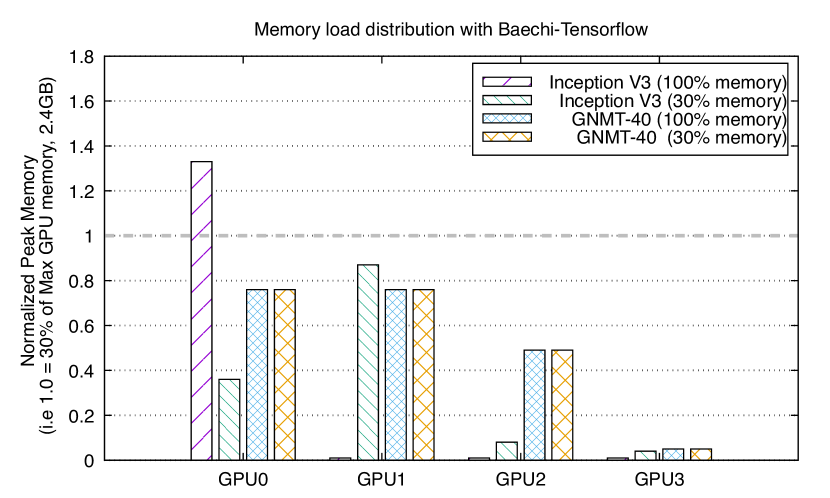
(a)

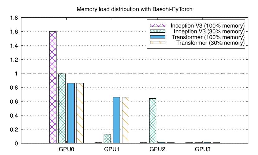
(b)

Figure 7. Baechi Load Balance of Memory Usage using m-SCT. Dashed line is memory limit for each GPU (normalized). Note that 1.0 on y axis corresponds to 30% of the max GPU memory (i.e. 2.4 GB in a 8 GB GPU)

Load Distribution. Figure 7 shows the peak memory usage, normalized to the memory limit for each GPU (insufficient memory case) for Baechi-TF and Baechi-PY. In both Baechi-TF and Baechi-PY, for Inception-V3,

with a 30% memory cap, a single GPU does not suffice, and that m-SCT relies on a mix of multiple GPUs. In particular, 2 of the 4 GPUs appear to be used more. This is because Inception-V3 has more barriers (sync points) than GNMT in TensorFlow, limiting Inception-V3’s ability to parallelize effectively.

For TensorFlow GNMT and PyTorch Transformer, Baechi’s m-SCT is able to load-balance more evenly (than Inception-V3) across the GPUs, even when memory is sufficient. In fact, for both these cases we found that m-SCT generates an identical placement in both cases with sufficient and with insufficient memory. This fact is also true for the expert, m-TOPO, and m-ETF. However specifically in case of GNMT with Baechi-TF, their step times are 2.6–3.2% higher than the sufficient memory cases (Table 4).This slowdown is because of TensorFlow runtime memory optimizations. Concretely, when the memory usage approaches its limit, the TensorFlow runtime resorts to certain memory optimizations to decrease peak memory usage. For the expert placement, peak memory usage for one GPU device decreases from 2 GB (83% of the memory limit) to 1.45 GB and thus the number of memory operations increases 6% under insufficient memory. These memory optimizations do not kick in for m-SCT, making it faster than the expert.

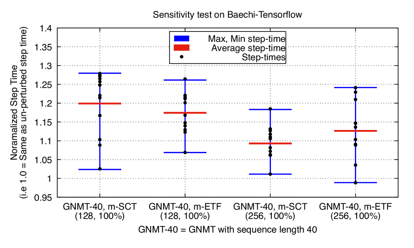
(a)

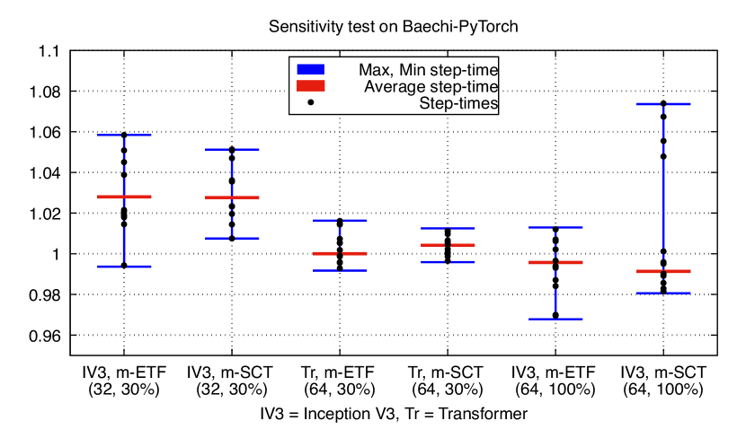
(b)

Figure 8. Baechi Sensitivity to Profiling Errors. All computation and communication times are perturbed randomly by up to 20% and the step time for placement generated by Baechi is measured. Values in X-axis parentheses are (Batch Size, Memory Fraction Available)

Profile Sensitivity. To measure Baechi’s sensitivity to profiling errors, we perform runs where in each run all computation and communication profiles are randomly and independently perturbed by up to $\pm$20%. This should account for errors in our time measurements as well as small speed differences between the device used to profile the model and devices where the model actually runs. Figure 8 shows the perturbation in step-times of the resulting placements, w.r.t. to step-time without any perturbation of the profiles. Compared to the unperturbed step times, the step times with perturbed profiles remain within a fraction of 0.99$\times$ to 1.3$\times$ in Baechi-TF, and between 0.97$\times$ and 1.08$\times$ times in Baechi-PY Thus we conclude that m-SCT and m-ETF are resilient to reasonable levels of errors in profiled values.

Benefit of Baechi Optimizations

Benefit of Baechi-TF Optimizations.

Table 6 shows the benefit from the combined optimizations of Section 3.1.2 and 3.1.3 in Baechi-TF. We use Inception-V3 with batch size 32 and GNMT with batch size of 128. We use the m-SCT variant of Baechi. The experimental setup has 4 GPUs with sufficient memory.

Table 6. Benefits of Baechi-TF Optimizations (Section 3.1.1). Number of Operators to be Placed, Placement Times in seconds, and Average Step Times in seconds. m-SCT.

Model	Un-Optimized			Optimized
	Num. Ops	Placement (seconds)	Step (seconds)	Num. Ops	Placement (seconds)	Step (seconds)
Inception-V3	6884	68.0	0.302	17	0.9	0.269
GNMT (length: 40)	18050	275.1	0.580	542	1.2	0.212
GNMT (length: 50)	22340	406.1	0.793	706	2.4	0.267

Table 7. Benefits of communication protocol in Baechi-PY (Section 3.2.2). Step times in seconds without and with the protocol

Model	Algorithm	Without Protocol	With Protocol	% Change
Inception V3 (32, 30% memory)	m-ETF	0.252	0.250	0.0%
	m-SCT	0.268	0.254	5.5%
Inception V3 (64, 40% memory)	m-ETF	0.551	0.528	4.3%
	m-SCT	0.550	0.535	2.8%
Transformer (64, 100% memory)	m-ETF	0.246	0.242	0.0%
	m-SCT	0.246	0.244	0.0%

Overall, we observe that Baechi-TF’s combined optimizations achieve 75.6$\times$–229.3$\times$ speedup in placement times, and 1.1$\times$–3.0$\times$ speedup in step times. We discuss a few interesting aspects. Operator fusion (Section 3.1.3) reduces both number of operators to be placed and thus also placement time. Forward-operator-based placement (Section 5) significantly speeds up placement. Concretely the latter optimization reduces the number of operators to be placed 2.7$\times$ for Inception-V3 and 6.5$\times$–7.0$\times$ for GNMT. This accelerates the placement times 13.7$\times$ for Inception-V3 and 20.2$\times$–31.4$\times$ for GNMT.

Co-placement (Section 3.1.2) is efficient because it clusters operators. This reduces step times. While co-placement does not change the operator count to be placed, it decreases placement time by reducing the overhead of calculating schedulable times.

Benefit of Baechi-PY Communication Protocol.

To evaluate the communication protocol in Baechi-PY (Section 3.2.2), we create a baseline plain wrapper. In it, each node transfers the inputs from devices of its parent (if different from module’s device) by simply using blocking calls to .to() instead of using streams. Table 7 shows the comparison of step times. Baechi-PY’s communication protocol gives up to 5.5% benefit with Inception-V3, and very little benefit under Transformer. This is because, in PyTorch, both these models have a strong linear spine, which creates fewer opportunities for parallelism.

Discussion and Limitations

Algorithmic Approaches vs Learning-based Approaches.

When we first implemented m-ETF and m-SCT, the placed models had very high step times because communication-intensive operators violated the SCT assumption (Table 1). We whittled away at this with a persistent effort at systems design and optimizations (outlined in Section 3.1), which played a major role in bringing the step times down. Although our exploration was efficient and we cycled new techniques and optimizations on a weekly basis, it took 1 person-year of effort to converge to what now appears in this paper for Baechi-TF, and an additional 1 person-year for Baechi-PY. This is indicative of the difficulties associated with implementing scheduling algorithms on today’s open-source ML systems (and in a sense shows why existing learning-based approaches are so attractive!). Nevertheless, our results show that the benefits of algorithmic design were worth the exploratory pain.

Our experience also indicates reasons why developers (and companies!) often choose to “jump” so quickly towards using learning-based (including RL-based) solutions for scheduling problems: fast time to design (optimization of parameters and hyperparameters can be often be done as a rote task, rather than a creative task), and hence fast time to production. However, this comes at the expense of latter pain points in generalizing learning-based approaches to different architectures and models (in comparison, Baechi runs as-is, given an arbitrary model and a machine profile), as well as the high times to generate a placement using learning-based approaches, which becomes a bottleneck in the exploratory design phase when the developer is iteratively building and revising their model. We conclude that learning-based techniques (for any problem) should not be built in isolation from, or in lieu of, algorithmic-based approaches—but rather hand-in-hand with them.

Limitations of Baechi-TF. The peak memory usage of TensorFlow is highly dependent on the execution order of operators (Ahn et al., 2020). So Baechi would benefit most if the framework (TensorFlow or PyTorch) faithfully executed operators in the same order as specified by Baechi’s ES. For Baechi-PY we enforce this via the “Reordering Problem” (Section 4.4). For TensorFlow while we do not enforce this ordering, and we observed in several runs of Baechi-TF that TensorFlow deviated from this order, yet memory caps were not violated for m-SCT and m-ETF in Baechi-TF runs. It is possible that if memory caps were tightened further (than 30%, compared to our experiments), engineering may be required for Baechi-TF to force TensorFlow to follow the ES execution order.

Limitations of Baechi-PY.

(i) Correctness issues with in-place operations: Inplace operations may lead to race conditions and incorrectness. Concretely, select modules in PyTorch can be made to modify the input tensors in-place, e.g., ReLU with in-place flag set. Baechi-PY’s communication protocol (in Section 3.2.2) uses an independent tx stream to move out the tensors from a device. If the subsequent module in the compute stream is in-place, it may modify the tensor while it is being transferred out. This may lead to an incorrect tensor. While we did not encounter such a cases in evaluation, a simple fix is to turn off the in-place feature for the module in question. This may however increase the memory consumption.

(ii) Weight sharing in Transformers: Currently the Assigner (Section 4.3) does not support cases where weights are shared across multiple modules in the model (e.g., Transformers with embedder weight sharing (Vaswani et al., 2017)).

(iii) Model code modifications: Some operations like concatenate and add, which take multiple inputs, must be defined as PyTorch modules. Only then can the Assigner ensure that tensors being concatenated or added are on the same device. In most cases, this is a few lines of code change. For instance, in Inception-V3, concatenate is used 7 times and add is used only once.

Related work

Data Parallelism (DP). Data parallelism (a.k.a. DP) refers to training the same model replicas with multiple partitioned data in parallel. This is motivated by increasing sizes of datasets. MALT (Li et al., 2015) is a fault-tolerant, network-cost effective solution for data parallel ML. Another common data parallelism framework is NESL (Bergstrom and Reppy, 2012), a first-order functional language that enables developers to put irregular-parallel program in parallel devices. OptiML (Sujeeth et al., 2011) is a domain-specific language (DSL). Most major ML frameworks offer support for data parallelism (Chen et al., 2015; Abadi et al., 2016; Paszke et al., 2019). While DP typically replicates the model on each device, ZeRO (Rajbhandari et al., 2020) eliminates this redundancy and reduces memory consumption in DP. DP is orthogonal to model parallelism, and therefore DP techniques can be integrated into Baechi.

Model Parallelism. Compared to data parallelism, relatively fewer solutions exist for model parallelism. DistBelief (Dean et al., 2012) and STRADS (Kim et al., 2016) require the user to manually specify device placement, while the systems in (Krizhevsky, 2014; Le, 2013) do not generalize to arbitrary ML models.

As discussed in Section 1, reinforcement-learning based approaches have been popular lately to perform placement for model parallelism, including work from Google (Mirhoseini et al., 2017, 2018) and the Placeto system (Addanki et al., 2019). ColocRL (Mirhoseini et al., 2017) trains a sequence-to-sequence model by RL to generate placements of manually grouped subsets of TensorFlow operators. HierarchicalRL (Mirhoseini et al., 2018) substitutes the human intervention for grouping operators with an ML model and jointly trains the ML models for operator grouping and device placements. Placeto (Addanki et al., 2019) proposes an approach that transfers learned device placement models to new ML models in order to minimize training times for the new model placements.

The original version of our paper (Jeon et al., 2020) both inspired follow-up work (Hafeez et al., 2021), and also had parallel work (Tarnawski et al., 2020), on algorithmic approaches to model parallelism. However (Tarnawski et al., 2020) is standalone, meaning that it is not integrated with TensorFlow or PyTorch, making a fair comparison with Baechi difficult. Pesto (Hafeez et al., 2021) presents direct comparisons with Baechi (Baechi-TF)—the most important metric of placement times are similar for Pesto and Baechi, with small improvements for step time. Thus for practical purposes we consider Pesto to be comparable in performance to Baechi.

Works like PipeDream (Harlap et al., 2018), GPipe (Huang et al., 2019), DAPPLE (Fan et al., 2021), PipeMare (Yang et al., 2021) introduce and optimize various aspects of Pipeline Parallelism. In Pipeline Parallelism, the model is usually vertically split into contiguous stages. Amazon Sagemaker recently introduced automating Model and Pipeline Parallelism on their platform recently, though their code is proprietary(Amazon, 2022a; Karakus et al., 2021). Techniques for pipeline parallelism can be integrated orthogonally into Baechi.

Model Parallelism for large language models. Recent progress on very large language models like GPT (Brown et al., 2020a, b) have given rise to works that focus specifically on Model Parallelism for such models like Megatron-LM (Shoeybi et al., 2019) and TeraPipe (Li et al., 2021). However, these systems focus narrowly on Transformer models. Alpa (Zheng et al., 2022) combines intra and inter-operator parallelism. The inter-operator parallelism is limited to vertical splits and will not, for instance, place multiple parallel branches of a model on different devices, thus making it different from model parallelism.

Classical Parallel Scheduling. Classical parallel scheduling, e.g., ETF (Hwang et al., 1989) and SCT (Hanen and Munier, 1995), has been widely used in task scheduling on multiple computers. ETF and SCT are used as baselines by many subsequent works (Eyraud-Dubois et al., 2015; Hu et al., 2010; Möhring et al., 1996; Veltman et al., 1990; Yang and Gerasoulis, 1994). None of these address memory constraints and a finite number of devices. For instance, Eyraud-Dubois et al. (Eyraud-Dubois et al., 2015) investigate the execution of tree-shaped task graphs using multiple processors, but without always obeying memory restrictions.

TensorFlow Graph Optimizations. Existing techniques (TensorFlow Community, 2022a, b) work only after the graph has been placed—e.g., to improve operations’ performance—and thus are inapplicable. E.g., Running Grappler (TensorFlow’s graph optimizer) generates an optimized graph protobuf, but it is unusable as it lacks certain metadata. Baechi’s targeted problem is harder as we have to both optimize the graph and do placement.

Conclusions

We have proposed algorithmic solutions to model parallelism, useful in scenarios where devices are memory-constrained or neural networks are massive. Among our three algorithms (m-ETF, m-TOPO, m-SCT), the m-SCT algorithm is provably within a constant factor of the optimal achievable training time. We have implemented these algorithms into our new Baechi system, as two systems Baechi-TF and Baechi-PY which are respectively usable in a modular manner with TensorFlow and PyTorch.

Experimental results showed that, across TensorFlow and PyTorch, our approaches reduce placement time by a factor of between $654\times$–$206000\times$ compared to today’s state-of-the-art placement approaches which are learning-based, while increasing step time (makespan) by only up to 6.2% compared to expert placers. When memory is constrained further, while single GPU and expert placers suffer OOM errors, Baechi’s algorithms, especially m-SCT and m-ETF, were able to place successfully. Compared to sufficient memory the step times suffered an increase of only up to 13.8% in TensorFlow and 16.1% in PyTorch. Further, Baechi-TF’s optimizations help reduce placement time by $75.6\times$–$229.3\times$, and step time by $1.1\times$–$3.0\times$. We also conclude that m-SCT and m-ETF perform comparably, with m-ETF having a slight edge for slower networks.

The original version of our paper (Jeon et al., 2020) inspired follow-up work (Hafeez et al., 2021) along with parallel work (Tarnawski et al., 2020), on algorithmic approaches to model parallelism. Together, this new generation of algorithms for model parallelism offers the promise of speed, generalizability, predictability, and analyzability. These will be invaluable as learning models, both training and inference, move closer to edge devices and human-facing devices.

Code. Baechi’s code is openly available at the following link:
http://dprg.cs.uiuc.edu/downloads.php

Appendix A Optimality Analysis for m-ETF

We now derive an upper bound on the makespan of graph $G$ running on $n$ memory-constrained devices according to a placement generated by m-ETF. A bound for ETF (with no memory constraint on the devices) was obtained in (Hwang et al., 1989). We extend it to the case where the devices have finite memory. For any given $p$ devices, let $\omega_{\textrm{m-etf}}^{p}$ be the m-ETF makespan and $\omega_{\textrm{opt}}^{p}$ be the optimal makespan achieved using devices with infinte memory and zero device-to-device communication costs.

Theorem 1.

The makespan of m-ETF, $\omega_{\textrm{m-etf}}^{n}$ is at most $(2+\rho)\omega_{\textrm{opt}}^{R}$, where $R$ is an integer $<n$ (computed in equation 11).

Proof.

Let $K=\displaystyle\frac{n\cdot M}{\sum_{i=1}^{m}d_{i}}$, where for any operator (task) $i$ in $G$, $d_{i}$ is the size of memory required by $i$. Intuitively, $K$ is the ratio of the total memory available from all devices to the total memory required by the model. Thus $K>1$, and for practical purposes we can assume that $K$ is sufficiently larger than 1. At each step, m-ETF greedily matches a ready task to an available device. Specifically, a device is said to be available if there is neither a task currently running nor has been scheduled to run on that device. A task is said to be ready if all of its predecessors have completed. Let $I$ and $A$ be the set of available devices and ready tasks at a given step respectively. When a task completes, $I$ is updated to include the recently free device and all of the task’s children that are ready are added to $A$.

At each such step, a device $d$ is said to be memory-sufficient (MS) if the remaining free memory on $d$ is greater than the memory requirement of each task in $A$. If $d$ has insufficient memory for even a single task in $A$, we say $d$ is not MS thereafter. It is removed from $I$ and is not considered for any further placement.

The time $(0,\omega_{\textrm{m-etf}})$ can be partitioned into two distinct sets. Set $\mathcal{A}$ containing the time-periods when all the MS devices (in that time-period) are busy and set $\mathcal{B}$ when at least one MS is idle. Suppose $\mathcal{B}$ is the disjoint union of intervals $(b_{li},b_{ri})$ i.e,

$$\mathcal{B}=(b_{l1},b_{r1})\cup(b_{l2},b_{r2})\cup\dots\cup(b_{lq},b_{rq})$$

where $b_{l1}<b_{r1}<b_{l2}<b_{r2}\dots<b_{lq}<b_{rq}$.

Lemma 0 (Theorem 3.2 in (Hwang et al., 1989)).

We can find a chain of tasks,

$$X:T_{l}\rightarrow T_{l-1}\rightarrow\dots\rightarrow T_{1}$$

such that

$$\sum_{i=1}^{q}(b_{r1}-b_{l1})\leq\sum_{j=1}^{l}t(T_{j})+\sum_{j=1}^{l-1}c_{j(j+1)}$$

That is, the total time period of $\mathcal{B}$ will be covered by computation and communication times along the chain $X$. We will denote $\sum_{j=1}^{l-1}c_{j(j+1)}$ by $C_{X}$. For proof, we refer the reader to Theorem 3.2 in (Hwang et al., 1989).

Let $r$ be the number of devices that remain MS until the end of m-ETF (i.e at time $\omega_{\textrm{m-etf}}$). With $K>1$, we will have $r>=1$. Let $\hat{\mathcal{B}}$ be the set of all time-periods when atleast one of these $r$ devices is idle. Note that $\hat{\mathcal{B}}\subseteq\mathcal{B}$, thus the chain $X$ from Lemma will cover $\hat{\mathcal{B}}$ as well. Thus we have:

(3) $$\sum_{r}t(\phi_{i})\;\leq\;r\times\sum_{T_{j}\in X}t(T_{j})\>+\>r\times C_{X}$$

where $\phi_{i}$ is the set of times when the device $d_{i}$ is idle in $(0,\omega_{\textrm{m-etf}})$ and $t(T)$ is computation time of task $T$.

Let $\omega_{\textrm{opt}}^{p}$ be the optimal makespan on $p$ devices with no memory limits and no communication costs. Since the makespan on any number of devices is at least as large as a chain in the graph, we have

(4) $$\omega_{\textrm{opt}}^{r}\;\geq\;\sum_{X}t(T_{j})\dots(i),\qquad\omega_{\textrm{opt}}^{n}\;\geq\;\sum_{X}t(T_{j})\dots(ii)$$

Also, the net computation time of $G$ can be bounded as:

(5) $$\sum_{T_{j}\in G}t(T_{j})\;\leq\;r\times\omega_{\textrm{opt}}^{r}\dots(i),\qquad\sum_{T_{j}\in G}t(T_{j})\;\leq\;n\times\omega_{\textrm{opt}}^{n}\dots(ii)$$

Now we bound the m-ETF makespan. Consider the $r$ devices, their idle time and the jobs running on them:

(6) $$\omega_{\textrm{m-etf}}^{n}\; =\;\frac{1}{r}\left(\sum_{r}t(T_{j})+\sum_{r}t(\phi_{i})\right)$$

(7) $$\leq\;\frac{1}{r}\left(\sum_{G}t(T_{j})+\sum_{r}t(\phi_{i})\right)$$

Using 3, 4(i) and 5(i),

$$\omega_{\textrm{m-etf}}^{n}\; \leq\;\frac{1}{r}\left(2r\times\omega_{\textrm{opt}}^{r}+r\times C_{X}\right)=\;2\omega_{\textrm{opt}}^{r}+C_{X}$$

Similarly, using 3, 4(ii) and 5(ii),

$$\omega_{\textrm{m-etf}}^{n}\; \leq\;\frac{1}{r}\left((n+r)\times\omega_{\textrm{opt}}^{n}+r\times C_{X}\right)=\;\left(\frac{n+r}{r}\right)\omega_{\textrm{opt}}^{n}+C_{X}$$

Note that $r$ will vary depending on the exact topological order considered for the m-ETF. So we define $R$ as the minimum $r$ across all possible topological ordering of the graph. Thus we have,

(8) $$\omega_{\textrm{m-etf}}^{n}\;\leq\;\min\left(2\omega_{\textrm{opt}}^{R},\;\left(\frac{n+R}{R}\right)\omega_{\textrm{opt}}^{n}\right)+C_{X}$$

Further, with $\rho$ as the ratio between maximum communication ttime and minimum computation time, we have $C_{X}\leq\rho\omega_{\textrm{opt}}^{n}$ (also $C_{X}\leq\rho\omega_{\textrm{opt}}^{R}$ )

Thus we have,

(9) $$\boxed{\omega_{\textrm{m-etf}}^{n}\;\leq\;\left(1+\frac{n}{R}+\rho\right)\omega_{\textrm{opt}}^{n}}$$

Alternatively, using the bound with $\omega_{\textrm{opt}}^{R}$,

(10) $$\boxed{\omega_{\textrm{m-etf}}^{n}\;\leq\;(2+\rho)\omega_{\textrm{opt}}^{R}}$$

Here we note that bound in Equation 10 is of the same form as the original bound on ETF given in (Hwang et al., 1989), where $R$ replaces $n$. Thus the makespan of m-ETF, like ETF, is within a constant factor of the optimal

Finally, $R$ can be computed as follows. Let the largest memory requirement of any task in $G$ be $J\times M$. Since the devices become non-MS when they can not place any of the available task in A , a memory of only $(1-J)M$ is use-able at each device in the worst case. Thus by greedily filling in the tasks onto devices, we get:

$$R\;\geq\;n-\left(\frac{\sum_{i=1}^{m}d_{i}}{(1-J)M}\right)\;=\;n-\frac{n}{(1-J)K}$$

Rounding it up, we have,

(11) $$R\;=\;\left\lceil n\left(1-\frac{1}{(1-J)K}\right)\right\rceil$$

∎

Appendix B Optimality Analysis of m-SCT

We now formally prove that m-SCT’s approximation ratio to optimal is an additive constant away from SCT’s approximation ratio. Since SCT itself was known to be within a constant factor of optimal (Hanen and Munier, 1995), our result means that m-SCT is also within a constant factor of optimal. Recall that we assume $\rho$ - the ration of maximum communication time to minimum computation time (defined in Table: 1) - is less than 1.

We will use similar notation to our analysis for m-ETF. Let $K=\displaystyle\frac{n\cdot M}{\sum_{i=1}^{m}d_{i}}$, where for any operator (task) $i$ in $G$, $d_{i}$ is the size of memory required by $i$. We will define $J$ as the ratio between largest memory requirement from a single task and $M$. Formally, $J=\max_{i\in[m]}\frac{d_{i}}{M}$.

Let $s_{i}$ be the start time of task $i$ in m-SCT, and $s_{i}^{\infty}$ be the start time of task i in the infinite device SCT algorithm. Let $u_{j}$ be the time where a task $j$ becomes urgent, which is exactly the earliest time when task $j$ can start on any device. Formally, $u_{j}=max_{i\rightarrow j\in E(G)}s_{i}+p_{i}+c_{ij}$.

Similar to m-ETF, we will say a device $d$ is memory sufficient (abbreviated as MS) at time $T$ if and only if remaining free memory on $d$ is greater than the memory requirement of each task in $A$. Finally, we will use $r$ to denote the number of devices that are MS throughout the scheduling process.

We will now analyse the approximation ratio of m-SCT with three steps. First we will show that not many tasks are impacted by devices going out of memory. Next we will show that any MS device must be idle only for a limited time. Our proof for this step follows a similar outline to the proof of Theorem 3 in (Hanen and Munier, 1995), but our proof is significantly shorter due to a condensed case analysis. Finally, we will bound the makespace of m-SCT by summing up the idle and busy time on MS devices.

Lemma 1.

There are at most $n-r$ task pairs $(i,j)$ such that $j$ is $i$’s favourite child, however when $j$ is scheduled, the device $d$ where $i$ is scheduled on does not have sufficient memory for task $j$.

Proof.

Since $i$ is scheduled on device $d$, $d$ must be memory sufficient when $i$ is scheduled, but is no longer memory sufficient sometime after $i$ is scheduled (since $d$ does not have sufficient memory for task $j$). Since there are in total $n$ devices and $r$ devices are always memory sufficient throughout m-SCT, there must only be $n-r$ events where a device transition from being memory sufficient to not memory sufficient. ∎

Lemma 2 (Variant of Lemma 6 in (Hanen and Munier, 1995)).

Given two time units $s^{\prime}\leq s$ such that $s-s^{\prime}\leq c_{max}$, let $i$ be a task such that $s_{i}\leq s^{\prime}\leq s_{i}+k_{i}+c_{max}$, then any busy or awake device at $s^{\prime}$ is free for at most $\max(s^{\prime}-s_{i},c_{max})$ time during $[s_{i},s]$.

Proof.

1. If a device $d$ is busy at $s^{\prime}$. Let task $a$ be the task that is running at time $s^{\prime}$. There are two possibilities:

   • If task $a$ started before $s_{i}$, then device $d$ is busy for at least $s^{\prime}-s_{i}$ time, thus free for at most $s-s^{\prime}\leq c_{max}$ time.

   • On the other hand, if task $a$ started at some time $s^{*}$ where $s_{i}\leq s^{*}\leq s^{\prime}$, then either task $a$ is still being executed at $s$, or task $a$ has completed at $s$. In the first case device $d$ is free for at most $s^{*}-s_{i}\leq s^{\prime}-s_{i}$ time. In the second case device $d$ is busy for at least $k_{a}\geq c_{max}\geq s-s^{\prime}$ time, and thus is free for at most $s-s_{i}-(s-s^{\prime})=s^{\prime}-s_{i}$ time.

   We conclude that device $d$ must be busy for at least $\min\{s^{\prime}-s_{i},s-s^{\prime}\}$ time during $[s_{i},s]$.

2. If a device is awake at $s^{\prime}$, let $a$ be the last task on $d$ before $s^{\prime}$ and let $s^{*}$ be when $a$ finishes. Then we know by the nature of our algorithm that some task $b$ will start on $d$ no later than $s^{*}+c_{max}$. Since $s-s^{\prime}\leq c_{max}$, we know that $b$ is not yet finished at time $s$. Therefore either task $a$ starts after $s_{i}$ (which means the device is busy for at least $k_{a}\geq c_{max}$ time and free for at most $s-s_{i}-c_{max}\leq s^{\prime}-s_{i}$ time), or the device is vacant for at most $c_{max}$ time.

∎

Lemma 3.

Assume that task $j$’s favourite parent $i^{*}$’s device is MS during time period $[s_{i},s_{j}]$. Then there exists a predecessor $i$ of $j$ such that the total amount of idle time during $[s_{i},s_{j}]$ on any device $d$ that is MS throughout the period is at most $s_{j}^{\infty}-s_{i}^{\infty}$.

Proof.

Note that since task $j$’s favourite predecessor $i^{*}$’s device is MS during $[s_{i},s_{j}]$, it is possible to schedule $j$ on the same device as $i^{*}$. This fact will be used in the case analysis.

Let $i$ be a predecessor of $j$ such that $s_{i}+k_{i}+c_{ij}$ is maximized (namely, $u_{j}=s_{i}+k_{i}+c_{ij}$). Notice also that after $j$ becomes urgent at $u_{j}$ and before $j$ is scheduled, all memory sufficient devices must be busy (otherwise $j$ would have been scheduled on a device). Hence for any $T<s_{j}$, the total vacant time for an MS device during $[T,s_{j}]$ is equal to its total vacant time during $[T,u_{j}]$. Now we will discuss three different scenarios and prove that in each scenario, an MS device is vacant for at most $s_{j}^{\infty}-s_{i}^{\infty}$ time during $[s_{i},s_{j}]$.

1. When $j$ is not the favorite child of $i$, we know that in the infinite device SCT algorithm, $i$ and $j$ are scheduled on different devices. Hence $s_{j}^{\infty}\geq s_{i}^{\infty}+k_{i}+c_{ij}$. On the other hand, in m-SCT, after $j$ becomes urgent ($j$ becomes urgent at time $s_{i}+k_{i}+c_{ij}$) and before $j$ is scheduled, any MS device must be busy. Therefore the amount of vacant time on each MS device during $[s_{i},s_{j}]$ must be at most $k_{i}+c_{ij}$.

2. When $j$ is the favorite child of $i$, but $i$’s device is not awake when task $i$ ends, we know that the time $j$ can be ready on $i$’s device is the same as $j$’s urgent time, which means there is another task $w$ such that $s_{w}+k_{w}+c_{wj}=s_{i}+k_{i}+c_{ij}$, but $j$ is not $w$’s favorite child. We can now use exactly the same argument as in the first case to prove that vacant time on any MS device during $[s_{i},s_{j}]$ must be at most $k_{i}+c_{ij}$.

3. When $j$ is the favorite child of $i$, and $i$’s device is awake when task $i$ ends. Denote the time $j$ becomes ready on $i$’s device as $ready(j)$, there must exist some $j$’s predecessor $y\neq i$ such that $s_{y}+k_{y}+c_{yj}=ready(j)$. Since $i$’s device is awake when task $i$ ends, task $j$ will be scheduled on $i$’s device if it is still idle by $ready(j)$. Hence a task $w$ (which is either $j$ or an urgent task) has to be scheduled on the device of $i$ at or before $ready(j)$. We will now consider the predecessor successor pair $(y,j)$, and prove that during $[s_{y},u_{j}]$ the vacant time on any MS machine is at most $s_{j}^{\infty}-s_{y}^{\infty}$.

   • If $w=j$, note that $j$ is not $y$’s favorite child. Hence in the infinite device SCT, $j$ and $y$ are not on the same device. We hence conclude that $s_{j}-s_{y}=ready(j)-s_{y}=k_{y}+c_{yj}\leq s_{j}^{\infty}-s_{y}^{\infty}$.

   • If $w\neq j$, then $w$ must be urgent (the only tasks that are allowed to be scheduled on an awake machine is the favorite child and urgent tasks). Hence at the start time of $w$, it must be the case that all MS devices are either busy or awake (because if there is a free MS device, k would have been scheduled on it). By Lemma 2, any busy or awake device at the start time of $w$ can only be vacant for at most $max(s_{w}-s_{y},c_{max})$ time during $[s_{y},u_{j}]$. Now we will upper bound $max(s_{w}-s_{y},c_{max})$ using the facts 1) $w$ happens before $ready(j)$, but after task $i$ is completed (namely, after $s_{i}+k_{i}$) and 2) $ready(j)-s_{y}\geq k_{y}\geq c_{max}$.

     $$max(s_{w}-s_{y},c_{max})\leq max(ready(j)-s_{y},c_{max})=ready(j)-s_{y}.$$

     Since in the infinite device SCT, $j$ and $y$ are not on the same device, we now conclude that the total vacant time on an MS device must be at most $ready(j)-s_{y}=k_{y}+c_{yj}\leq s_{j}^{\infty}-s_{y}^{\infty}$.

∎

Lemma 4.

Assume that task $j$’s favourite parent $i^{*}$’s device is not MS during time period $[s_{i},s_{j}]$. Then there exists a predecessor $i$ of $j$ such that the total amount of idle time during $[s_{i},s_{j}]$ on any device $d$ that is MS throughout the period is at most $s_{j}^{\infty}-s_{i}^{\infty}+c_{ij}$.

Proof.

As argued in Lemma 3, any MS device must be busy after $u_{j}$. Let $i$ be a predecessor of $j$ such that $s_{i}+k_{i}+c_{ij}$ is maximized (namely, $u_{j}=s_{i}+k_{i}+c_{ij}$). Then $u_{j}-s_{i}=k_{i}+c_{ij}\leq s_{j}^{\infty}-s_{i}^{\infty}+c_{ij}$ (because even with infinite number of devices, task $i$ must be fully executed before task $j$ starts). ∎

Let $R$ be the minimum $r$ across all possible graph configurations with memory availability parameter $K$. We will use $\omega_{\textrm{m-sct}}^{p}$ and $\omega_{\textrm{sct}}^{p}$ to denote the makespan of m-SCT (with memory limit) and SCT (without memory limit) with $p$ devices respectively. Analogously, we will use $\omega_{\textrm{m-opt}}^{p}$ and $\omega_{\textrm{opt}}^{p}$ be the optimal makespan on $p$ devices with memory limit and with no memory limit respectively. We will use $\alpha$ to denote the approximation of the infinite device SCT (against the optimal makespan with infinite devices).

Theorem 5.

The makespan of m-SCT is at most $(\frac{p}{R}+\alpha)\cdot\omega_{\textrm{opt}}^{p}+\frac{(n-R)}{R}\cdot c_{max}$ for any $p$.

Proof.

Let $D_{MS}$ be the set of all devices that are MS throughout the m-SCT algorithm. We know that $|D_{MS}|=r$. It is clear that the total amount of computation time spent on devices in $D_{MS}$ is at most the sum of computational time for all tasks, which is at most $\omega_{\textrm{opt}}^{r}\cdot r$.

Now we will count the amount of time a device $d\in D_{MS}$ is idle. WLOG, let $T_{1}$ be the task that finishes last in m-SCT and let $T_{l}\rightarrow T_{l-1}\rightarrow\cdots\rightarrow T_{1}$ be the chain of task in $G$ ending at $T_{1}$ such that $T_{l}$ is a source. Before the start time $s_{l}$ of $T_{l}$, all MS devices must be busy, because $T_{l}$ is urgent from time $0$ and would have been scheduled on a device as soon as it becomes idle. Let $n_{d}$ be the number of task pairs $(i,j)$ such that $i$ is $j$’s favourite parent but $i$’s parent is not MS when task $j$ starts. By Lemma 1, 3 and 4 we know that during $[s_{l},\omega_{\textrm{m-sct}}^{p}]=[s_{l},s_{1}+k_{1}]$ ($s_{1}$, $k_{1}$ are the start time and computation time of $T_{1}$ respectively) , the amount of time $d$ is idle is at most

$$\left\lparen\sum_{j=1}^{l-1}\left\lparen s_{j}^{\infty}-s_{j+1}^{\infty}\right\rparen\right\rparen+n_{d}\cdot c_{max}\leq\omega_{\textrm{sct}}^{\infty}+n_{d}\cdot c_{max}.$$

Summing these all up for all devices in $D_{MS}$ we get that the total idle time across all devices in $D_{MS}$ is at most

$$r\cdot\omega_{\textrm{sct}}^{\infty}+(n-r)\cdot c_{max}.$$

We now conclude that

$$r\cdot\omega_{\textrm{m-sct}}^{p} \leq r\cdot\omega_{\textrm{opt}}^{r}+r\cdot\omega_{\textrm{sct}}^{\infty}+(n-r)\cdot c_{max}$$

$$\Rightarrow\omega_{\textrm{m-sct}}^{p} \leq\omega_{\textrm{opt}}^{r}+\omega_{\textrm{sct}}^{\infty}+\frac{n-r}{r}\cdot c_{max}$$

$$\leq\omega_{\textrm{opt}}^{r}+\alpha\cdot\omega_{\textrm{opt}}^{\infty}+\frac{n-r}{r}\cdot c_{max}$$

$$\leq\omega_{\textrm{opt}}^{R}+\alpha\cdot\omega_{\textrm{opt}}^{\infty}+\frac{n-R}{R}\cdot c_{max}\quad\text{(because $R\leq r$)}.$$

Lastly, observe that (without memory limit), the optimal makespan with $R$ devices is at most $\frac{p}{R}$ times the optimal makespan with $p$ devices. Also, $\omega_{\textrm{opt}}^{\infty}\leq\omega_{\textrm{opt}}^{R}$. Hence $\omega_{\textrm{m-sct}}^{n}\leq(\frac{p}{R}+\alpha)\cdot\omega_{\textrm{opt}}^{p}+\frac{(n-R)}{R}\cdot c_{max}$. One could minimize the RHS over all $p$ to get the best upper bound. ∎

Using the same analysis as for m-ETF, we know that

$$R\;=\;\left\lceil n\left(1-\frac{1}{(1-J)K}\right)\right\rceil.$$