PDE constrained shape optimisation with first-order and Newton-type methods in the $W^{1,\infty}$ topology

Abstract

We present a general shape optimisation framework based on the method of mappings in the $W^{1,\infty}$ topology. We propose steepest descent and Newton-like minimisation algorithms for the numerical solution of the respective shape optimisation problems. Our work is built upon previous work of the authors in Deckelnick, Herbert, and Hinze, ESAIM: COCV 28 (2022), where a $W^{1,\infty}$ framework for star-shaped domains is proposed. To illustrate our approach we present a selection of PDE constrained shape optimisation problems and compare our findings to results from so far classical Hilbert space methods and recent $p$-approximations.

1 Introduction

This work considers the use of vector-valued Lipschitz continuous functions in the task of optimising shapes. The use of Lipschitz functions for shape optimisations is not necessarily new, having appeared in [DHH22] in a limited setting of star-shaped domains. While it may be possible to formulate many problems in a star-shaped setting, it lacks the natural formulation which is useful to practitioners, therefore making uptake in the community less likely. Recent work which aimed to approximate this Lipschitz approach used a $p$-Laplacian. Of course one is interested in the limit $p\to\infty$, however it can prove troublesome to utilise significantly large $p$ in computation. Our approach will not require the use of degenerate elliptic operators, but remain appropriate for the implementation by practitioners and will appear in upcoming work. This article will not concern itself with an extensive analysis of the convergence of the proposed algorithms, but will focus on the ease of implementation and examples. A particular novelty which we consider is the use of second order data in this Lipschitz setting for which we demonstrate an effective algorithm for its implementation in this shape context. An analysis for a model problem with a first order method is presented within [DHH23]. The second order method we present, or some variety of it would be very interesting to analyse.

We are interested in the numerical solutions of a number of shape optimisation problems

$$\min\mathcal{J}(\Omega),\,\Omega\in\mathcal{S},$$ (1)

where $\mathcal{S}$ is a collection of admissible domains. This collection and the functional $\mathcal{J}$ will vary depending on the application. To find, at least local, minima of this problem, we will consider a descent method. By this, we mean that, given $\Omega\in\mathcal{S}$, we seek $V^{*}\colon\mathbb{R}^{n}\to\mathbb{R}^{n}$ such that $\mathcal{J}^{\prime}(\Omega)[V^{*}]<0$ and set $\Omega_{\rm new}=({\rm id}+\alpha V^{*})(\Omega)$ for some suitably chosen $\alpha>0$. To ensure that the map $\operatorname{id}+\alpha V^{*}$ is a homeomorphism, it is sufficient to restrict to $\alpha$ to be small enough that $\alpha|DV^{*}|<1$ a.e., where, $|\cdot|$ is pointwise the spectral (operator) norm. While it is sufficient to take any sub-multiplicative norm, the spectral norm is convenient as it relates the Lipschitz and $W^{1,\infty}$ semi-norms.

In the literature, it is common to seek $V^{*}$ in a Hilbert space $H$ which represents the negative gradient i.e.

$$(V^{*},\eta)_{H}=(-\nabla_{H}\mathcal{J}(\Omega),\eta)_{H}:=-\mathcal{J}^{\prime}(\Omega)[\eta]$$ (2)

for all $\eta\in H$, or equivalently, one might seek

$$V^{*}\in\operatorname*{arg\,min}\left\{\frac{1}{2}\|V\|_{H}^{2}+\mathcal{J}^{\prime}(\Omega)[V]:V\in H\right\}.$$ (3)

A crucial issue in this context is the regularity of the solution $V^{*}$ to problem (3), which strongly depends on the regularity of the current domain $\Omega$ as well as the choice of $H$. It for example is not clear whether $\operatorname{id}+\alpha V^{*}$ defines a Lipschitz transformation for many frequent choices of $H$. In order to avoid these issues it was suggested in [DHH22] to work directly in the space $W^{1,\infty}(\Omega,\mathbb{R}^{d})$ and to consider the following problem

$$V^{*}\in\operatorname*{arg\,min}\left\{\mathcal{J}^{\prime}(\Omega)[V]:V\in W^{1,\infty}(\Omega,\mathbb{R}^{d}),|DV|\leq 1\mbox{ a.e. in }\Omega\right\}.$$ (4)

In [DHH22] this idea was analysed and implemented for shape optimisation problems involving star-shaped domains. It is the purpose of this paper to extend this approach to more general domains including the use of Newton–type methods.

Literature

There continues to be rapid development in the mathematical and numerical analysis of shape optimisation. The seminal works of Delfour and Zolésio [DZ11], Sokolowski and Zolésio, and the recent overview by Allaire, Dapogny, and Jouve [ADJ21] and the comprehensive bibliographies within provide an extensive overview of the topic of shape optimisation. The analysis, both mathematical and numerical, of shape optimisation problems has an extensive history, see e.g. [Bel+97, GM94, MS76, Sim80]. While computational power has increased in recent years, it has encouraged further development of shape optimisation [SSW15, SSW16, SW17], particularly fluid dynamical applications [Ben+15, Fis+17, Gar+15, Gar+18, RCP16, HUU20, HSU21, Küh+19, Sch+13]. Many articles have considered different choices of inner products on Hilbert spaces. A variety of choices are presented in [HPS15]. One particularly interesting example is [ISW18] which uses a penalty to weakly enforce the Cauchy-Riemann equations however it only appears applicable in two dimensions. Another category of interesting choices are reproducing kernel Hilbert spaces [ES18], which for certain kernels, one may provide an explicit shape gradient. While in a Hilbertian setting, the work [OS21] considers non-smooth terms to ensure that a mesh does not become degenerate. Some methods very much target having a particularly good mesh, a particular example is the so-called pre-shape calculus [LS21a, LS21].

The utilisation of Banach spaces for shape optimisation is gathering attention. To the best of our knowledge this was introduced in [DHH22] and considered $W^{1,\infty}$ perturbations for a star-shaped setting. The direction of steepest descent in a star-shaped setting has been linked to optimal transport [Her23]. The star-shaped setting is frequently exploited [EHS07, BCS21] to allow for a deeper analysis at the expense of generality. A $p$-approximation to the infinity problem (4) is utilised in [Mül+21] to optimise a fluid dynamic problem using a $p$-Laplace relaxation. Such a fluid problem is frequently discussed in shape optimisation as it is known [Pir74] that, for Stokes flow, the optimal shape should have a tip. In [Mül+21], experiments demonstrate that the $p$-method will form a tip as opposed to in more classical Hilbertian methods. The article [Mül+22] develops upon [Mül+21] to consider the computational scalability of a method closely related to a $p$-Laplace relaxation of (4).

Higher order methods are also of interest and will be considered in this work; second order methods have been considered in [SS23], utilising a so-called linear version of the second shape derivative.

Outline

We begin in Section 2 by outlining some necessary definitions and results for shape optimisation, mentioning the Lagrange approach from optimisation to write down first and second derivatives and providing examples which we will consider. We then move onto a discussion about the discretisation of the infinity method in Section 4. Section 5 then provides numerical experiments of the previously described numerical experiments using the novel $W^{1,\infty}$ method we discuss.

2 Shape derivatives and Lagrangian calculus

2.1 Preliminaries

In what follows we denote by $D\subset\mathbb{R}^{d}$ a convex hold-all domain. We consider the shape optimisation problem

$$\min\mathcal{J}(\Omega),\,\Omega\in\mathcal{S},$$ (5)

where $\mathcal{S}$ is a collection of admissible domains such that $\Omega\Subset D$ for all $\Omega\in\mathcal{S}$. Here, we use the symbol $\Subset$ to denote compactly contained. It is not difficult to see that $\operatorname{id}+V$ is a bi-Lipschitz transformation from $D$ to $D$ provided that $V\in W_{0}^{1,\infty}(D,\mathbb{R}^{d})$ with $\|DV\|_{L^{\infty}}<1$. Assuming that $(\operatorname{id}+V)(\Omega)\in\mathcal{S}$ for such $V$ we say that $\mathcal{J}$ is shape differentiable at $\Omega$ if (cf. [ADJ21, Definition 4.1]) $V\mapsto\mathcal{J}\bigl{(}(\operatorname{id}+V)(\Omega)\bigr{)}$ is Fréchet–differentiable at $V=0$ as a mapping from $W_{0}^{1,\infty}(D,\mathbb{R}^{d})$ into $\mathbb{R}$. An update step in a descent algorithm based on the Fréchet derivative of $\mathcal{J}$ will then seek a direction $V\in W_{0}^{1,\infty}(D,\mathbb{R}^{d})$ such that $\mathcal{J}^{\prime}(\Omega)[V]<0$. In order to determine the direction of steepest descent we are led to the problem of finding $V^{*}\in W_{0}^{1,\infty}(D,\mathbb{R}^{d})$ with

$$V^{*}\in\operatorname*{arg\,min}\left\{\mathcal{J}^{\prime}(\Omega)[V]:V\in W_{0}^{1,\infty}(D,\mathbb{R}^{d}),|DV|\leq 1\mbox{ a.e. in }D\right\}.$$ (6)

Let us note that we are including the hold-all domain within this minimisation problem for the determination of a direction of steepest descent, along with a Dirichlet boundary condition on the boundary of the hold-all domain. Note that the fact that $D$ is convex ensures that $V$ is a Lipschitz continuous function with Lipschitz constant $1$. Using the direction (6) within a descent algorithm hence requires the solution of a highly nontrivial constrained minimisation problem which can be approximated at the discrete level with the help of an alternating direction method of multipliers (ADMM).

The above approach will lead to a first order method. If $\mathcal{J}$ is twice shape differentiable, it is worthwhile considering a Newton–type approach as well. This can be achieved by replacing the minimisation problem (6) by

$$\min\left\{\frac{t}{2}\mathcal{J}^{\prime\prime}(\Omega)[V,V]+\mathcal{J}^{\prime}(\Omega)[V]:V\in W_{0}^{1,\infty}(D;\mathbb{R}^{d}),\,|DV|\leq 1\mbox{ a.e. in }D\right\},$$ (7)

where $t>0$ may be interpreted as a damping factor. Here, the evaluation of $\mathcal{J}^{\prime\prime}(\Omega)$ is by no means straightforward and we will use the Lagrangian calculus described in the next subsection to carry out the calculations for the class of problems that we are interested in. Our motivation for the formulation of (7) is the following approximation: for $t\in(-1,1)$ and $V\in W_{0}^{1,\infty}(D;\mathbb{R}^{d})$ with $|DV|\leq 1$ a.e. in $D$ it holds that

$$\mathcal{J}((\operatorname{id}+tV)(\Omega))=\mathcal{J}(\Omega)+t\mathcal{J}^{\prime}(\Omega)[V]+\frac{t^{2}}{2}\mathcal{J}^{\prime\prime}(\Omega)[V,V]+\mbox{higher order terms}.$$ (8)

Throwing away these higher order terms and minimising over the admissible $V$, we recover (7).

Under appropriate conditions, one may show the existence of solutions of (6) and (7), the approach being similar to results presented in [PWF18] and [DHH22]. In Theorem 1 we verify the existence of solutions with some reasonable assumptions. In a discrete setting, the assumptions given for the continuous case are trivially satisfied.

2.2 Lagrangian framework for PDE–constrained optimisation

For the ease of exposition, let us consider a shape functional of the form

$$\mathcal{J}(\Omega)=\int_{\Omega}j(\cdot,y_{\Omega})\,{\rm d}x,$$ (9)

where $j\colon D\times\mathbb{R}\rightarrow\mathbb{R}$ is assumed to be sufficiently smooth and $y_{\Omega}$ denotes the solution of a PDE posed in $\Omega$. Let us note that one may also consider the gradient of the solution in the functional $\mathcal{J}$ which follows very similarly, but adds a layer of complexity to the already large formulae. We shall adapt the Lagrangian framework developed in Sections 1.6.4 and 1.6.5 of [Hin+08] in order to compute $\mathcal{J}^{\prime}(\hat{\Omega})$ and $\mathcal{J}^{\prime\prime}(\hat{\Omega})$ at a fixed domain $\hat{\Omega}\Subset D$. The main aspect of the Lagriangian method is to, in effect, decouple the state, $y_{\Omega}$, from, in the setting we consider, the shape, $\Omega$. Denoting by $B$ a small open neighbourhood of $0$ in $W_{0}^{1,\infty}(D,\mathbb{R}^{d})$ we associate with $V\in B$ the perturbed domain $\Omega_{V}:=(\operatorname{id}+V)(\hat{\Omega})$. By transforming to $\hat{\Omega}$ we find that, for the choice made in (9), $\mathcal{J}(\Omega_{V})=J(V,y_{\Omega_{V}}\circ(\operatorname{id}+V))$, where

$$J(V,y):=\int_{\hat{\Omega}}j(\operatorname{id}+V,y)\det(\operatorname{I}+DV)\,{\rm d}\hat{x},$$ (10)

and we note that $|\det(\operatorname{I}+DV)|=\det(\operatorname{I}+DV)$ if $|DV|$ is sufficiently small. The derivatives of this choice of $J$ may be found in Appendix A.1. In order to incorporate the PDE constraint we let $y=y_{\Omega_{V}}\circ(\operatorname{id}+V)$ and suppose that $y_{\Omega_{V}}$ solves the given PDE problem on $\Omega_{V}$ if and only if $e(V,y)=0$ for some mapping $e\colon B\times X\rightarrow Z$. Here, $X$, $Z$ are suitable function spaces on $\hat{\Omega}$ and we assume in what follows that $e_{y}(0,\hat{y})\colon X\rightarrow Z$ is invertible, where $\hat{y}=y_{\hat{\Omega}}$. After choosing $B$ smaller if necessary to apply an Implicit Function Theorem, there exists for every $V\in B$ a unique $y=y(V)\in X$ such that $e(V,y(V))=0$, so that we may write

$$\mathcal{J}(\Omega_{V})=J(V,y(V))$$

where, in the context of optimal control, the map $V\mapsto\mathcal{J}(\Omega_{V})$ takes the role of a reduced cost functional. In order to calculate the derivatives of $\mathcal{J}$ it is convenient to introduce the Lagrange functional $L\colon X\times B\times Z^{*}\to\mathbb{R}$

$$L(y,V,p)={J(V,y)}+\langle p,e(V,y)\rangle,$$ (11)

so that

$$\mathcal{J}(\Omega_{V})=L(y(V),V,p)\quad\mbox{ for any }p\in Z^{*}.$$

If we denote by $p(V)$ the solution of $L_{y}(y(V),V,p(V))=0$, one immediately obtains that

$$\mathcal{J}^{\prime}(\hat{\Omega})[V]=L_{V}(\hat{y},0,\hat{p})[V],$$ (12)

where $\hat{p}=p(0)$. In a similar way one finds for the second derivative

$$\mathcal{J}^{\prime\prime}(\hat{\Omega})[V,W] = L_{yy}(\hat{y},0,\hat{p})[y^{\prime}(0)[V],y^{\prime}(0)[W]]+L_{yV}(\hat{y},0,\hat{p})[V,y^{\prime}(0)[W]]$$

$$+L_{Vy}(\hat{y},0,\hat{p})[y^{\prime}(0)[V],W]+L_{VV}(\hat{y},0,\hat{p})[V,W],$$

where $y^{\prime}(0)[V]$ is the derivative of $W\mapsto y(W)$ at $W=0$ in direction $V\in W^{1,\infty}_{0}(D,\mathbb{R}^{d})$, which satisfies

$$\langle p,e_{y}(0,\hat{y})[y^{\prime}(0)[V]]\rangle=-\langle p,e_{V}(0,\hat{y})[V]\rangle,\quad\mbox{ for all }p\in Z^{*}.$$ (13)

For the implementation of the Newton-like method in (7), it is necessary to evaluate $\mathcal{J}^{\prime\prime}(\hat{\Omega})[V,W]$ many times. In order to carry out the corresponding calculations as efficiently as possible we would like to avoid the frequent evaluation of $y^{\prime}(0)[W]$. To do, let us write

$$\mathcal{J}^{\prime\prime}(\hat{\Omega})[V,W]=\langle h_{1},y^{\prime}(0)[W]\rangle+\langle h_{2},W\rangle,$$

where

$$\langle h_{1},y\rangle = L_{yy}(\hat{y},0,\hat{p})[y^{\prime}(0)[V],y]+L_{yV}(\hat{y},0,\hat{p})[V,y],$$

$$\langle h_{2},W\rangle = L_{Vy}(\hat{y},0,\hat{p})[y^{\prime}(0)[V],W]+L_{VV}(\hat{y},0,\hat{p})[V,W].$$

We then first define $g\in Z^{*}$ as the solution of

$$\langle g,e_{y}(0,\hat{y})[y]\rangle=\langle h_{1},y\rangle\quad\forall y\in X$$ (14)

and then set

$$\langle h_{3},W\rangle=-\langle g,e_{V}(0,\hat{y})[W]\rangle,\quad W\in W_{0}^{1,\infty}(D,\mathbb{R}^{d}).$$

This gives

$$\mathcal{J}^{\prime\prime}(\hat{\Omega})[V,W] = \langle h_{1},y^{\prime}(0)[W]\rangle+\langle h_{2},W\rangle=\langle g,e_{y}(0,\hat{y})[y^{\prime}(0)[W]]\rangle+\langle h_{2},W\rangle$$

$$= -\langle g,e_{V}(0,\hat{y})[W]\rangle+\langle h_{2},W\rangle=\langle h_{2}+h_{3},W\rangle.$$

The evaluation of $\mathcal{J}^{\prime\prime}(\hat{\Omega})[V,\cdot]$ hence essentially requires the solutions of (13) and of the adjoint problem (14).

2.3 Existence of descent-like directions

Now it is demonstrated how to construct the first and second derivatives, we demonstrate the well-posedness of the problem given in (7). The result is very similar to those which appear in [PWF18] and [DHH22]

Theorem 1.

Given $t\geq 0$, suppose that the maps

$$V\mapsto \mathcal{J}^{\prime}(\Omega)[V]\mbox{ and}$$ (15)

$$V\mapsto t\mathcal{J}^{\prime\prime}(\Omega)[V,V]$$ (16)

are weak-$*$ lower-semi-continuous, then there exists

$$V^{*}\in\operatorname*{arg\,min}\left\{\frac{t}{2}\mathcal{J}^{\prime\prime}(\hat{\Omega})[V,V]+\mathcal{J}^{\prime}(\hat{\Omega})[V]:V\in W^{1,\infty}_{0}(D;\mathbb{R}^{d}),\,|DV|\leq 1\right\}.$$ (17)

Proof.

Consider a sequence $\{V_{n}\}_{n=1}^{\infty}\subset\{V\in W^{1,\infty}_{0}(D;\mathbb{R}^{d}):|DV|\leq 1\}$ such that

$$\frac{t}{2}\mathcal{J}^{\prime\prime}(\hat{\Omega})[V_{n},V_{n}]+\mathcal{J}^{\prime}(\hat{\Omega})[V_{n}]\searrow\\ \searrow\inf\left\{\frac{t}{2}\mathcal{J}^{\prime\prime}(\hat{\Omega})[V,V]+\mathcal{J}^{\prime}(\hat{\Omega})[V]:V\in W^{1,\infty}_{0}(D;\mathbb{R}^{d}),\,|DV|\leq 1\right\}\mbox{ as }n\nearrow\infty.$$ (18)

It holds that $V_{n}$ is bounded, hence there is a weak-$*$ convergent subsequence, say $\{V_{n_{k}}\}_{k=1}^{\infty}$, and limit $V^{*}\in W^{1,\infty}_{0}(D;\mathbb{R}^{d})$ such that $|DV_{h}^{*}|\leq 1$ a.e. in $D$ and $V_{n_{k}}\overset{*}{\rightharpoonup}V^{*}$ in $W^{1,\infty}_{0}(D;\mathbb{R}^{d})$. Furthermore, by the assumed weak-$*$ lower-semi-continuity of $t\mathcal{J}^{\prime\prime}(\hat{\Omega})[V,V]$ and $\mathcal{J}^{\prime}(\hat{\Omega})[V]$, we have that $V^{*}$ is a minimiser. ∎

Let us briefly discuss the assumptions above. The condition that $V\mapsto\mathcal{J}^{\prime}(\Omega)[V]$ is weak-$*$ lower-semi-continuous is typically verified in practice by observing that there is $g_{0}\in L^{1}(\Omega;\mathbb{R}^{d})$ and $g_{1}\in L^{1}(\Omega;\mathbb{R}^{d\times d})$ such that

$$\mathcal{J}^{\prime}(\Omega)[V]=\int_{\Omega}\left(g_{0}\cdot V+g_{1}:DV\right){\rm d}x,$$ (19)

which provides weak-$*$ continuity. The second condition is more tricky. As we have seen in Section 2.2 that the construction of the second derivative is non-trivial, as such the condition is less easy to explicitly check. However it is the case that, if the mapping $V\mapsto\mathcal{J}^{\prime\prime}(\Omega)[V,V]$ non-negative, then it holds that it is weak-$*$ lower semi-continuous. This certainly depends on the shape optimisation problem at hand. However it is perhaps not too unreasonable to assume that, near a minimiser, the second derivative of the energy is non-negative.

3 Example shape optimisation problems

Here, we now discuss a few example shape optimisation problems.

3.1 Poisson problem

As a first PDE constraint we here consider the Poisson problem. We set $X=H^{1}_{0}(\hat{\Omega})$ and $Z=X^{*}$. Since we are in a reflexive setting, we use the canonical injection and identify $Z^{*}$ with $X$. By $y_{\Omega}$ we denote the solution of

$$-\Delta y_{\Omega}=F\mbox{ in }{\Omega},\quad y_{\Omega}=0\mbox{ on }\partial{\Omega}$$ (20)

for a given $F\in L^{2}(D)$. In particular, we find that $y_{\Omega_{V}}\circ(\operatorname{id}+V)$ is a solution of $e(V,y)=0$ where $e\colon B\times H^{1}_{0}(\hat{\Omega})\rightarrow H^{-1}(\hat{\Omega})$ is given by

$$\langle e(V,y),p\rangle=\int_{\hat{\Omega}}\left(A(V)\nabla y\cdot\nabla p-F\circ(\operatorname{id}+V)p\right)\det(\operatorname{I}+DV)\,{\rm d}\hat{x},\quad p\in H^{1}_{0}(\hat{\Omega}),$$ (21)

and $A(V):=(\operatorname{I}+DV)^{-1}(\operatorname{I}+DV)^{-T}$. Derivatives of the map $e$ may be found in Appendix A.2.1. With the Lagrange functional

$$L(V,y,p)=\int_{\hat{\Omega}}j(\operatorname{id}+V,y)\det(\operatorname{I}+DV)\,{\rm d}\hat{x}+\langle e(V,y),p\rangle$$

we deduce from (12) the well–known formula

$$\mathcal{J}^{\prime}(\hat{\Omega})[V] = L_{V}(\hat{y},0,\hat{p})[V]$$

$$= \int_{\hat{\Omega}}\left(j(\cdot,\hat{y})\operatorname{div}V+j_{x}(\cdot,\hat{y})\cdot V+\mathcal{A}[V]\nabla\hat{y}\cdot\nabla\hat{p}-\hat{p}\operatorname{div}(FV)\right)d\hat{x},$$

where

$$\mathcal{A}[V]:=\operatorname{I}\operatorname{div}V-DV-DV^{T},$$ (23)

$\hat{y}\in H^{1}_{0}(\hat{\Omega})$ satisfies $e(0,\hat{y})=0$, and the adjoint $\hat{p}\in H^{1}_{0}(\hat{\Omega})$ satisfies $L_{y}(\hat{y},0,\hat{p})=0$, i.e.

$$\int_{\hat{\Omega}}\nabla\hat{p}\cdot\nabla\eta\,{\rm d}\hat{x}=-\int_{\hat{\Omega}}j_{y}(\cdot,\hat{y})\eta\,{\rm d}\hat{x}\quad\mbox{ for all }\eta\in H^{1}_{0}(\hat{\Omega}).$$ (24)

3.2 Bi-Laplace-type equation

Let us next consider the minimsation of $\mathcal{J}$ as in (9) subject to the linear PDE of fourth order

$$\Delta^{2}y_{\Omega}=F\mbox{ in }\Omega,\quad y_{\Omega}=\Delta y_{\Omega}=0\mbox{ on }\partial\Omega.$$ (25)

If the boundary of $\Omega$ is sufficiently regular the above problem can be split into two second order Poisson problems by introducing $-\Delta y_{\Omega}$ as an additional variable. Let us note that this splitting is analytically useful to ensure that the shape derivative exists in the sense of [ADJ21, Definition 4.1], due to the fourth order nature of the problem. Let us comment that this need not be necessary since the shape differentiability, particularly boundedness in Lipschitz functions, with a fourth order constraint was demonstrated in [EH22] in a surface context, while [Las17] shows this for a fourth order eigenvalue problem.

On the fixed domain, we set $X=\left(H^{1}_{0}(\hat{\Omega})\right)^{2}$ and $Z=X^{*}$. Again we will use the canonical injection to identify $Z^{*}$ with $X$. Posing the split formulation of (25) on $\Omega_{V}$ and transforming it back onto $\hat{\Omega}$ in the same way as above we write the map $e$ which represents the PDE constraint as,

$$\langle e(V,y),p\rangle = \int_{\hat{\Omega}}\bigl{(}A(V)\nabla y_{1}\cdot\nabla p_{2}-y_{2}p_{2}\bigr{)}\det(\operatorname{I}+DV)\,{\rm d}\hat{x}$$ (26)

$$+\int_{\hat{\Omega}}\bigl{(}A(V)\nabla y_{2}\cdot\nabla p_{1}-F\circ(\operatorname{id}+V)p_{1}\bigr{)}\det(\operatorname{I}+DV)\,{\rm d}\hat{x},$$

for all $y=(y_{1},y_{2}),p=(p_{1},p_{2})\in\left(H_{0}^{1}(\hat{\Omega})\right)^{2}$. Derivatives of the map $e$ may be found in Appendix A.2.2. Similar to (3.1) we obtain for the shape derivative

$$\mathcal{J}^{\prime}(\hat{\Omega})[V] = \int_{\hat{\Omega}}\left(j(\cdot,\hat{y}_{1})\operatorname{div}V+j_{x}(\cdot,\hat{y}_{1})\cdot V+\mathcal{A}[V]\nabla\hat{y}_{1}\cdot\nabla\hat{p}_{2}-\hat{y}_{2}\hat{p}_{2}\operatorname{div}V\right)\,{\rm d}\hat{x}$$ (27)

$$+\int_{\hat{\Omega}}\left(\mathcal{A}[V]\nabla\hat{y}_{2}\cdot\nabla\hat{p}_{1}-\operatorname{div}(FV)\hat{p}_{1}\right)\,{\rm d}\hat{x},$$

where $\hat{y}=(\hat{y}_{1},\hat{y}_{2})\in\left(H^{1}_{0}(\hat{\Omega})\right)^{2}$ satisfies $e(0,\hat{y})=0$ and the adjoint $\hat{p}=(\hat{p}_{1},\hat{p}_{2})\in(H^{1}_{0}(\hat{\Omega}))^{2}$ satisfies

$$\int_{\hat{\Omega}}\nabla\hat{p}_{2}\cdot\nabla\eta_{1}\,{\rm d}\hat{x} =-\int_{\hat{\Omega}}j_{y}(\cdot,\hat{y}_{1})\eta_{1}\,{\rm d}\hat{x}\quad\forall\eta_{1}\in H^{1}_{0}(\hat{\Omega}),$$ (28)

$$\int_{\hat{\Omega}}\nabla\hat{p}_{1}\cdot\nabla\eta_{2}\,{\rm d}\hat{x} =\int_{\hat{\Omega}}\hat{p}_{2}\eta_{2}\,{\rm d}\hat{x}\quad\forall\eta_{2}\in H^{1}_{0}(\hat{\Omega}).$$ (29)

3.3 Optimisation of the first eigenvalue for the Laplacian

Our aim is to apply the above Lagrangian framework also for the optimisation of the first Dirichlet eigenvalue of the Laplacian, i.e.

$$\mathcal{J}(\Omega)=\lambda_{1}(\Omega),$$ (30)

where $\lambda_{1}(\Omega)$ is defined by

$$\lambda_{1}(\Omega):=\inf\left\{\int_{\Omega}|\nabla z|^{2}\,{\rm d}x:z\in H^{1}_{0}(\Omega),\,\int_{\Omega}z^{2}\,{\rm d}x=1\right\}.$$ (31)

With the notation of Section 2.2 we again fix a $\hat{\Omega}\Subset D$ which we now assume to be connected and set $\Omega_{V}=(\operatorname{id}+V)(\hat{\Omega})$. We transform the eigenvalue relation

$$-\Delta z_{\Omega_{V}}=\lambda z_{\Omega_{V}}\mbox{ in }\Omega_{V},\quad z_{\Omega_{V}}=0\mbox{ on }\partial\Omega_{V}$$

together with the condition $\int_{\Omega_{V}}z_{\Omega_{V}}^{2}{\rm d}x=1$ onto $\hat{\Omega}$ and write it in the form $e(V,y)=0$, where $e\colon B\times X\rightarrow Z$, with $X=H^{1}_{0}(\hat{\Omega})\times\mathbb{R},Z=X^{*}$, and

$$\langle e(V,y),p\rangle = \int_{\hat{\Omega}}\left(A(V)\nabla z\cdot\nabla q-\lambda zq\right)\,\det(\operatorname{I}+DV)\,{\rm d}\hat{x}$$ (32)

$$+\mu\left(1-\int_{\hat{\Omega}}z^{2}\,\det(\operatorname{I}+DV)\,{\rm d}\hat{x}\right),$$

for $y=(z,\lambda),p=(q,\mu)\in H^{1}_{0}(\hat{\Omega})\times\mathbb{R}$. Derivatives of the map $e$ may be found in Appendix A.2.3. Let $\hat{z}\in H^{1}_{0}(\hat{\Omega})$ be an eigenfunction to the first Dirichlet eigenvalue $\hat{\lambda}$ with $\int_{\hat{\Omega}}\hat{z}^{2}\,{\rm d}x=1$. Then we have for all $p=(q,\mu)\in H^{1}_{0}(\hat{\Omega})\times\mathbb{R}$

$$\langle e_{V}(0,\hat{y})[V],p\rangle= \int_{\hat{\Omega}}\left(\mathcal{A}[V]\nabla\hat{z}\cdot\nabla q-\hat{\lambda}\operatorname{div}V\hat{z}q-\mu\operatorname{div}V\hat{z}^{2}\right)\,{\rm d}\hat{x},$$ (33)

$$\langle e_{y}(0,\hat{y})[(\eta,\tilde{\eta})],p\rangle= \int_{\hat{\Omega}}\left(\nabla\eta\cdot\nabla q-\hat{\lambda}\eta q-\tilde{\eta}\hat{z}q-2\mu\hat{z}\eta\right)\,{\rm d}\hat{x},$$ (34)

where $\hat{y}=(\hat{z},\hat{\lambda})$. Since $\hat{\lambda}$ is simple, cf. $\hat{\Omega}$ is connected and $\hat{\lambda}$ is the first Dirichlet eigenvalue [Gil+77, Theorem 8.38], it can be shown that $e_{y}(0,\hat{y})\colon H^{1}_{0}(\hat{\Omega})\times\mathbb{R}\rightarrow H^{-1}(\hat{\Omega})\times\mathbb{R}$ is invertible. Thus we can write for $V\in B$

$$\mathcal{J}(\Omega_{V})=J(V,y(V)),\quad\mbox{ where }J(V,(z,\lambda))=\lambda.$$

The Lagrange functional is given by $L(y,V,p)=\lambda+\langle e(V,y),p\rangle$ so that we derive with the help of (3.1)

$$\mathcal{J}^{\prime}(\hat{\Omega})[V]=L_{V}(\hat{y},0,\hat{p})[V]=\langle e_{V}(0,\hat{y})V,\hat{p}\rangle.$$ (35)

The adjoint $\hat{p}=(\hat{q},\hat{\mu})$ is given by the relation $L_{y}(\hat{y},0,\hat{p})=0$, i.e.

$$\tilde{\eta}+\int_{\hat{\Omega}}\left(\nabla\eta\cdot\nabla\hat{q}-\hat{\lambda}\eta\hat{q}-\tilde{\eta}\hat{z}\hat{q}-2\hat{\mu}\hat{z}\eta\right){\rm d}\hat{x}=0\quad\forall(\eta,\tilde{\eta})\in H^{1}_{0}(\hat{\Omega})\times\mathbb{R}.$$

We infer that $\int_{\hat{\Omega}}\hat{z}\hat{q}\,d\hat{x}=1$ as well as

$$\int_{\hat{\Omega}}\left(\nabla\eta\cdot\nabla\hat{q}-\hat{\lambda}\eta\hat{q}\right){\rm d}\hat{x}=2\hat{\mu}\int_{\hat{\Omega}}\hat{z}\eta\,{\rm d}\hat{x}\quad\forall\eta\in H^{1}_{0}(\hat{\Omega}).$$

Choosing $\eta=\hat{z}$ we deduce that $\hat{\mu}=0$, so that $\hat{q}$ is an eigenfunction for the eigenvalue $\hat{\lambda}$. Since $\hat{\lambda}$ is simple and $\int_{\hat{\Omega}}\hat{z}\hat{q}\,{\rm d}\hat{x}=1$ we infer that $\hat{q}=\hat{z}$ and hence by (35) that (cf. [Hen06, HP18])

$$\lambda_{1}^{\prime}(\hat{\Omega})[V]=\int_{\hat{\Omega}}\left(\mathcal{A}[V]\nabla\hat{z}\cdot\nabla\hat{z}-\hat{\lambda}\operatorname{div}V\hat{z}^{2}\right){\rm d}\hat{x}.$$ (36)

It is known that the first eigenvalue scales with volume, as such we are interested in fixing the volume of $\Omega$. While it is known that the minimiser of the first eigenvalue is a ball, the methodology is interesting and can be applied to more complicated eigenvalue problems.

4 Discretisation

Our aim is to formulate a descent algorithm which produces in each step a polygonal domain and which replaces a possible PDE constraint with a corresponding finite element approximation. To begin, let $\mathcal{T}_{h}^{0}$ be a triangulation of the hold–all domain $D$. We look for discrete directions of descent in the finite element spaces

$$\mathcal{V}_{h}^{n}:=\left\{V_{h}\in C^{0}(\overline{D};\mathbb{R}^{d}):V_{h}|_{T}\in P^{1}(T;\mathbb{R}^{d}),\,\forall T\in\mathcal{T}_{h}^{n},\,V_{h}=0\mbox{ on }\partial D\right\},$$ (37)

where $P^{1}(T;\mathbb{R}^{d})$ denotes polynomials of degree at most one on $T$ with values in $\mathbb{R}^{d}$ and $\mathcal{T}_{h}^{n}$ is to be determined for $n\geq 1$. With a polygonal initial domain, $\Omega_{0}$ which is a union of the triangles in the triangulation $\mathcal{T}_{h}^{0}$, we will set $\Omega_{n+1}=(\operatorname{id}+t_{n}V_{n})(\Omega_{n})$ for $n\geq 1$, where $t_{n}\in(0,1)$ is a step size and we will shortly explain how to choose $V_{n}\in\mathcal{V}_{h}^{n}$. As well as updating the domain, the triangulation will also be updated, $\mathcal{T}^{n+1}_{h}=\{(\operatorname{id}+t_{n}V_{n})(T):T\in\mathcal{T}_{h}^{n}\}$. By the choice of $\mathcal{V}_{h}^{n}$ and the fact that $V_{n}$ will satisfy $|DV_{n}|\leq 1$, it holds that the updated mesh will be admissible since $t_{n}\in(0,1)$.

4.1 Choice of descent direction

Let $n\geq 0$ be fixed and let us denote the polygonal domain $\hat{\Omega}=\Omega_{n}\Subset D$ which is a union of triangles in $\mathcal{T}_{h}^{n}$. For simplicity we will henceforth neglect the dependence on $n$. Given $t\geq 0$, we aim to find $V_{h}^{*}\in\mathcal{V}_{h}$ such that

$$V_{h}^{*} \in \operatorname*{arg\,min}\left\{\frac{t}{2}\mathcal{J}^{\prime\prime}(\hat{\Omega})_{h}[V_{h},V_{h}]\mathcal{J}^{\prime}(\hat{\Omega})_{h}[V_{h}]:V_{h}\in\mathcal{V}_{h},|DV_{h}|\leq 1\mbox{ a.e. in }D\right\}$$

$$= \operatorname*{arg\,min}\left\{\int_{D}\phi(DV_{h}){\rm d}x+\frac{t}{2}\mathcal{J}^{\prime\prime}(\hat{\Omega})_{h}[V_{h},V_{h}]+\mathcal{J}^{\prime}(\hat{\Omega})_{h}[V_{h}]:V_{h}\in\mathcal{V}_{h}\right\}.$$

In this setting, $\mathcal{J}^{\prime}(\hat{\Omega})_{h}$ and $\mathcal{J}^{\prime\prime}(\hat{\Omega})_{h}$ are suitable approximations of $\mathcal{J}^{\prime}(\hat{\Omega})$ and $\mathcal{J}^{\prime\prime}(\hat{\Omega})$ respectively. The function $\phi$ is given by

$$\phi(A):=\begin{cases}0,&|A|\leq 1,\\ \infty,&|A|>1.\end{cases}$$ (38)

The approximations of the shape derivatives of $\mathcal{J}(\Omega)$ may be given in many forms, it may not be the case that one wishes to take the shape derivative of the discrete energy, one may prefer to do some post-processing. This leads to discussions of order of discretisation and optimisation which we do not wish to include here.

Let us now state that there exists a solution. The proof of which is almost identical to that of Theorem 1.

Theorem 2.

Given fixed $h>0$ and $t\geq 0$, there exists

$$V_{h}^{*}\in\operatorname*{arg\,min}\left\{\frac{t}{2}\mathcal{J}^{\prime\prime}(\hat{\Omega})_{h}[V_{h},V_{h}]+\mathcal{J}^{\prime}(\hat{\Omega})_{h}[V_{h}]:V_{h}\in\mathcal{V}_{h},\,|DV_{h}|\leq 1\right\}.$$ (39)

Unlike before, we did not need to make conditions on $\mathcal{J}^{\prime}(\hat{\Omega})_{h}$ or $\mathcal{J}^{\prime\prime}(\hat{\Omega})_{h}$, this is due to the finite dimensional nature ensures that the existence of a strongly convergengent subsequence of an infimising sequence.

Let us comment that the question of in what way and with which estimates does $V_{h}^{*}$ converge as $h\to 0$ is open. In [Bar21], a problem similar to the case $t=0$ is considered. Using discontinuous elements, the author was able to provide estimates on the energy. Let us note that this lack of estimate is not expected to be prohibitive to an initial analysis of our proposed algorithm.

In order to find the function $V_{h}^{*}$, we use an alternating direction method of multipliers (ADMM) approach in order to solve the above problem. To do so, we set

$$\mathcal{Q}_{h}:=\left\{q_{h}\in L^{2}(D;\mathbb{R}^{d\times d}):q_{h}|_{T}\in P^{0}(T;\mathbb{R}^{d\times d}),\,\forall T\in\mathcal{T}_{h}\right\}$$ (40)

and consider for a given $\tau>0$ the functional $\mathcal{L}_{\tau}\colon\mathcal{V}_{h}\times\mathcal{Q}_{h}\times\mathcal{Q}_{h}\rightarrow\mathbb{R}$ with

$$\begin{split}\mathcal{L}_{\tau}(V_{h},q_{h};\lambda_{h}):=&\int_{D}\left(\phi(q_{h})+\lambda_{h}:(DV_{h}-q_{h})\right){\rm d}x+\frac{\tau}{2}\|DV_{h}-q_{h}\|_{L^{2}(D;\mathbb{R}^{d\times d})}^{2}\\ &+\frac{t}{2}\mathcal{J}^{\prime\prime}(\hat{\Omega})_{h}[V_{h},V_{h}]+\mathcal{J}^{\prime}(\hat{\Omega})_{h}[V_{h}].\end{split}$$ (41)

The idea of ADMM is to alternatively minimise $\mathcal{L}_{\tau}$ over $q_{h}$ and $V_{h}$, then perform an update to $\lambda_{h}$ and repeat this until a certain quantity is small. More precisely, the algorithm has the following form:

Algorithm 3.

0. Choose $V^{0}_{h}$ and $\lambda^{0}_{h}$ such that $\mathcal{J}^{\prime}(\hat{\Omega})_{h}[V^{0}_{h}]<\infty$
1. Set $R=\infty$, $j=1$
While $R>tol$:
2. Find $q^{j}_{h}\in\operatorname*{arg\,min}\{\mathcal{L}_{\tau}(V^{j-1}_{h},q_{h};\lambda^{j-1}_{h}):q_{h}\in\mathcal{Q}_{h},|q_{h}|\leq 1\}$
3. Find $V^{j}_{h}\in\operatorname*{arg\,min}\{\mathcal{L}_{\tau}(V_{h},q^{j}_{h};\lambda^{j-1}_{h}):V_{h}\in\mathcal{V}_{h}\}$
4. Set $\lambda^{j}_{h}=\lambda^{j-1}_{h}+\tau(DV^{j}_{h}-q^{j}_{h})$
5. Set $R=\left(\|\lambda^{j}_{h}-\lambda^{j-1}_{h}\|_{L^{2}(D;\mathbb{R}^{d\times d})}^{2}+\tau^{2}\|DV^{j}_{h}-DV^{j-1}_{h}\|_{L^{2}(D;\mathbb{R}^{d\times d})}^{2}\right)^{\frac{1}{2}}$
6. Update j = j+1

Let us also mention [BM20] which considers more general ADMM methods with variable $\tau$. Particularly, in our experiments we make use of such an algorithm with variable $\tau$, namely [BM20, Algorithm 3.19].

In a finite dimensional setting, since we have the existence of minimisers, c.f. Theorem 2, it is almost immediate that Algorithm 3 converges. It is necessary to check the sign of $\mathcal{J}^{\prime\prime}(\Omega)_{h}$; in the locality of a minimiser, one might expect that it is non-negative.

Theorem 4 (ADMM converges).

Suppose that $t\in[0,1)$ and $t\mathcal{J}^{\prime\prime}(\hat{\Omega})_{h}$ is a non-negative operator, then it holds that Algorithm 3 converges.

This follows from [HY15]. The assumption that $t\mathcal{J}^{\prime\prime}(\Omega)_{h}$ is non-negative is made in order to ensure the appropriate functional is convex, which is a sufficient condition for the convergence of ADMM.

4.2 Evaluation of $\mathcal{J}^{\prime}(\hat{\Omega})_{h}$

4.2.1 PDE–constrained shape optimisation

Let us formulate suitable approximations of the shape derivatives derived in 2.2. Given the polygonal domain $\hat{\Omega}$ we denote by $\mathbb{S}_{h}(\hat{\Omega})$ the space of linear finite elements on $\hat{\Omega}$ (resolved by a subtriangulation of $\mathcal{T}_{h}$) which vanish on $\partial\hat{\Omega}$. If the constraint is given by (20) we set

$$\mathcal{J}^{\prime}(\hat{\Omega})_{h}[V_{h}]=\int_{\hat{\Omega}}\left(j(\cdot,\hat{y}_{h})\operatorname{div}V_{h}+j_{x}(\cdot,\hat{y}_{h})\cdot V_{h}+\mathcal{A}[V_{h}]\nabla\hat{y}_{h}\cdot\nabla\hat{p}_{h}-\hat{p}_{h}\operatorname{div}(FV_{h})\right){\rm d}\hat{x},$$ (42)

for $V_{h}\in\mathcal{V}_{h}$, where $\hat{y}_{h},\hat{p}_{h}\in\mathbb{S}_{h}(\hat{\Omega})$ satisfy

$$\begin{split}\int_{\hat{\Omega}}\nabla\hat{y}_{h}\cdot\nabla\eta_{h}\,{\rm d}\hat{x}=&\int_{\hat{\Omega}}F\eta_{h}\,{\rm d}\hat{x}\quad\forall\eta_{h}\in\mathbb{S}_{h}(\hat{\Omega}),\\ \int_{\hat{\Omega}}\nabla\hat{p}_{h}\cdot\nabla\eta_{h}\,{\rm d}\hat{x}=&-\int_{\hat{\Omega}}j_{y}(\cdot,\hat{y}_{h})\eta_{h}\,{\rm d}\hat{x}\quad\forall\eta_{h}\in\mathbb{S}_{h}(\hat{\Omega}).\end{split}$$ (43)

On the other hand, if the constraint is given by (25) then we let

$$\begin{split}\mathcal{J}^{\prime}(\hat{\Omega})_{h}[V_{h}]=&\int_{\hat{\Omega}}\left(j(\cdot,\hat{y}_{h,1})\operatorname{div}V_{h}+j_{x}(\cdot,\hat{y}_{h,1})\cdot V_{h}+\mathcal{A}[V]\nabla\hat{y}_{h,1}\cdot\nabla\hat{p}_{h,2}-\hat{y}_{h,2}\hat{p}_{h,2}\operatorname{div}V_{h}\right)\,{\rm d}\hat{x}\\ &+\int_{\hat{\Omega}}\left(\mathcal{A}[V_{h}]\nabla\hat{y}_{h,2}\cdot\nabla\hat{p}_{h,1}-\operatorname{div}(V_{h}F)\hat{p}_{h,1}\right)\,{\rm d}\hat{x},\end{split}$$ (44)

for $V_{h}\in\mathcal{V}_{h}$. Here, $\hat{y}_{h}=(\hat{y}_{h,1},\hat{y}_{h,2})\in(\mathbb{S}_{h}(\hat{\Omega}))^{2}$ satisfies

$$\int_{\hat{\Omega}}\nabla\hat{y}_{h,1}\cdot\nabla\eta_{h}\,{\rm d}\hat{x} =\int_{\hat{\Omega}}\hat{y}_{h,2}\eta_{h}\,{\rm d}\hat{x}\quad\forall\eta_{h}\in\mathbb{S}_{h}(\hat{\Omega}),$$ (45)

$$\int_{\hat{\Omega}}\nabla\hat{y}_{h,2}\cdot\nabla\eta_{h}\,{\rm d}\hat{x} =\int_{\hat{\Omega}}F\eta_{h}\,{\rm d}\hat{x}\quad\forall\eta_{h}\in\mathbb{S}_{h}(\hat{\Omega})$$ (46)

while $\hat{p}_{h}=(\hat{p}_{h,1},\hat{p}_{h,2})\in(\mathbb{S}_{h}(\hat{\Omega}))^{2}$ satisfies

$$\int_{\hat{\Omega}}\nabla\hat{p}_{h,2}\cdot\nabla\eta_{h}\,{\rm d}\hat{x} =-\int_{\hat{\Omega}}j_{y}(\cdot,y_{h,1})\eta_{h}\,{\rm d}\hat{x}\quad\forall\eta_{h}\in\mathbb{S}_{h}(\hat{\Omega}),$$ (47)

$$\int_{\hat{\Omega}}\nabla\hat{p}_{h,1}\cdot\nabla\eta_{h}\,{\rm d}\hat{x} =\int_{\hat{\Omega}}\hat{p}_{h,2}\eta_{h}\,{\rm d}\hat{x}\quad\forall\eta_{h}\in\mathbb{S}_{h}(\hat{\Omega}).$$ (48)

4.2.2 Optimisation of the first eigenvalue for the Laplacian

For a given polygonal domain we determine $\hat{z}_{h}\in\mathbb{S}_{h}(\hat{\Omega})$ and $\hat{\lambda}_{h}>0$ such that $\int_{\hat{\Omega}}\hat{y}_{h}^{2}\,{\rm d}x=1$ and

$$\hat{\lambda}_{h}=\inf\left\{\int_{\hat{\Omega}}|\nabla\hat{z}_{h}|^{2}\,{\rm d}\hat{x}:\hat{z}_{h}\in\mathbb{S}_{h}(\hat{\Omega}),\,\int_{\hat{\Omega}}\hat{z}_{h}^{2}\,{\rm d}\hat{x}=1\right\}=\int_{\hat{\Omega}}|\nabla\hat{z}_{h}|^{2}\,{\rm d}\hat{x}.$$

Supposing that the eigenvalue $\lambda_{h}$ is simple we let, recalling (36)

$$\mathcal{J}^{\prime}(\hat{\Omega})_{h}[V_{h}]=\int_{\hat{\Omega}}\left(\mathcal{A}[V_{h}]\nabla\hat{z}_{h}\cdot\nabla\hat{z}_{h}-\hat{\lambda}_{h}\hat{z}_{h}^{2}\operatorname{div}V_{h}\right)\,{\rm d}\hat{x}\mbox{ for }V_{h}\in\mathcal{V}_{h}.$$ (49)

5 Numerical experiments

We now provide numerical experiments for the applications we have described. In the integrals for the energy we use quadrature of order 2, while for the shape derivatives, we are using the order which is automatically decided by the software.
As mentioned above we will solve the state and adjoint PDEs with a finite element approximation. The finite element approximation is performed with DUNE [Bas+21], making particular use of the DUNE Python bindings [DNK20, DN18]. We consider a construction of update direction using four different approaches. Our approaches will be:

• The direction of steepest descent method using the $W^{1,\infty}$-topology, constructed with an adaptive ADMM method, as mentioned after Algorithm 3. This will be referred to as $p=\infty$.

• A Newton-type direction, which will be a discrete minimiser of (7) for a given $t>0$, referred to as the Newton method. Much like the $p=\infty$ case above, this will be constructed with an adaptive ADMM method.

• To compare against existing approaches, for $p=2,4$, we will consider the minimiser of $\mathcal{V}_{h}\ni V_{h}\mapsto\mathcal{J}^{\prime}(\Omega)_{h}+\frac{1}{p}\int_{D}|DV_{h}|^{p}{\rm d}x$. In the case that $p=2$, this is seen to coincide with the discrete case of (3) with $H=H^{1}_{0}(D;\mathbb{R}^{d})$ with the Dirichlet inner product. We will refer to these cases by their $p$ value.

The discrete functions produced by the $p=2$ and $p=4$ methods will be normalised so that they have a $W^{1,\infty}(D;\mathbb{R}^{d})$ semi-norm of $1$. This normalisation is performed so that we need not check whether the mesh has overlapped. For each of the experiments, we will set the hold-all domain to be the box $D=(-2,2)^{2}$. With these directions, we will move the vertices of our mesh according to an Armijo step rule. We will stop after 20 shape updates have been made. In most cases the domain has become close to stationary at this point and the Armijio step-size has become rather small.

The energy along the iterations will be plotted. In the case that the minimiser is known, the origin will be offset by the known value, when the minimiser is not known, the origin will be offset by the smallest value attained in the experiment.

5.1 Minimisation without a PDE constraint

Here we will consider that there is no PDE constraint, so that the map $e$ need not be included. We comment that the no PDE example may be derived as an example from the following Section 5.2 where one chooses right hand side data $F=0$ so that the state constraint guarantees $y=0$.

For this experiment, the main contributions to the error is that induced by the quadrature rules when calculating the energy and the shape derivative, as well as the direction of descent with the chosen method.

5.1.1 No PDE experiment 1

For this problem, we consider

$$j(x,y)=-Z(x)$$ (50)

where

$$Z(x)=\begin{cases}\cos(0.5\pi x_{1})\cos(0.5\pi x_{2})&|x_{1}|\mbox{ and }|x_{2}|\leq 1,\\ \frac{\pi}{4}(1-x_{1}^{2})&|x_{1}|>1\mbox{ and }|x_{2}|<1,\\ \frac{\pi}{4}(1-x_{2}^{2})&|x_{1}|<1\mbox{ and }|x_{2}|>1,\\ \frac{\pi}{4}(2-x_{1}^{2}-x_{2}^{2})&\mbox{otherwise}.\end{cases}$$ (51)

For the Newton direction we take $t=0.0625$. One expects the square $(-1,1)^{2}$ to be a minimiser of $\mathcal{J}$. It holds that $\mathcal{J}\left((-1,1)^{2}\right)=-\frac{16}{\pi^{2}}$. We start with the initial domain $(-1.5,-1)\times(-1,1)$. The triangulation of the domain and hold-all is displayed in Figure 1(a). In Figure 1(b), the energy of shapes along the minimising sequences we produce are given.

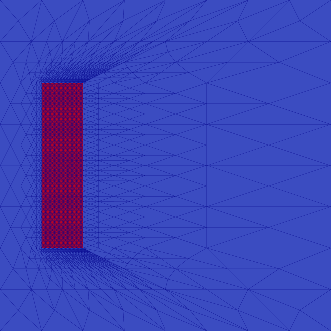
(a) Initial domain for the first No PDE experiment in Section 5.1.1, with $(-1.5,-1)\times(-1,1)$ in red and the hold-all, $(-2,2)^{2}$ in blue.

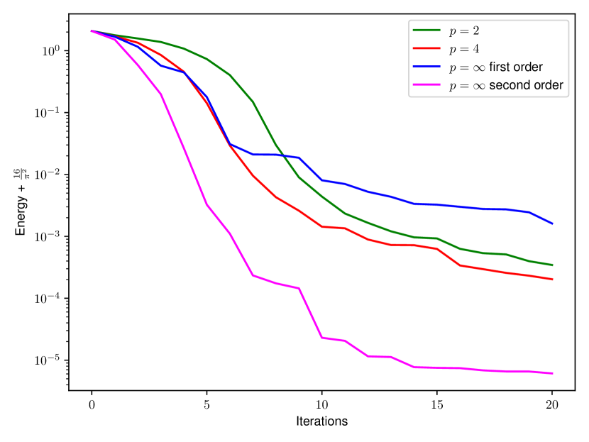
(b) Graph of the energy for the iterates in the first No PDE experiment in Section 5.1.1. It is seen that the Newton-type method is energetically performing the best while the first order infinity method appears to struggle compared to the traditional $p=2$ method.

Figure 1: Initial mesh and graph of the energy for the experiment in Section 5.1.1.

In Figure 2, the meshes of the final domains $\Omega$ for each of the methods are given.

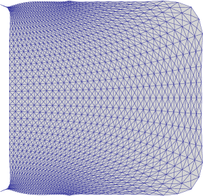
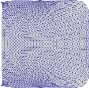
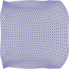
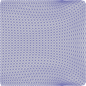
Figure 2: The meshes of $\Omega$ for the final domains produced in the first No PDE experiment in Section 5.1.1: top left to bottom, $p=2,4,\infty$ and second order. Due to symmetry of the result, we show only a half of each mesh. It is seen that none of the methods correctly captures the corners which are expected from the minimising shape. This is unsurprising as there is not a particularly large influence of the energy around the corners, where $Z$ is quite close to zero. The Newton-type method is the closest to forming corners.

5.1.2 No PDE experiment 2

For this problem, we consider

$$j(x,y)=\frac{1}{2}Z(x)^{2}$$ (52)

where for given $\epsilon>0$,

$$Z(x)=\sqrt{(x_{1}+x_{2})^{2}+\epsilon}+\sqrt{(x_{1}-x_{2})^{2}+\epsilon}$$ (53)

is a smooth approximation to $|x_{1}+x_{2}|+|x_{1}-x_{2}|$. For the Newton direction we take $t=0.125$. A very similar experiment with the non-smooth energy was considered in [DHH22]. This smooth approximation is used because we intend to employ the Newton method for which it would be useful to have (weak) second derivatives of $Z$. Without any constraint, we know that the theoretical minimiser is degenerate, a measure zero set. To avoid this, we will fix the area to be constrained equal to $4$. We expect this to have minimiser close to the square $(-1,1)^{2}$ which, for $\epsilon=0$, has energy $4$. Our directions of descent will only preserve the area constraint in a linear sense by restricting to $V$ with $\int_{\Omega}\operatorname{div}V=0$. We will perform a projection step to fix the area after each update.

We take $\epsilon=10^{-4}$ and start with an approximation of a ball of radius $\frac{2}{\sqrt{\pi}}$ at the origin. The triangulation of the domain and hold-all is displayed in Figure 3(a). In Figure 3(b), the energy of shapes along the minimising sequences we produce are given.

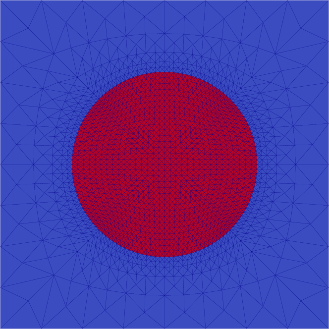
(a) Initial domain for the second No PDE experiment in Section 5.1.2, an approximation of the ball of radius $\frac{2}{\sqrt{\pi}}$ at the origin, is in red and the hold-all, $(-2,2)^{2}$ in blue.

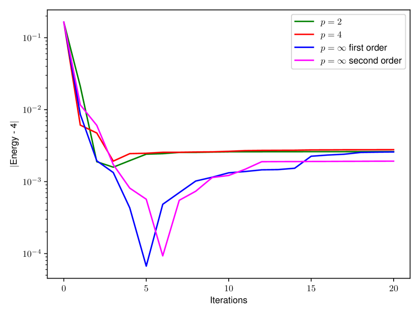
(b) Graph of the energy for the iterates in the second No PDE experiment in Section 5.1.2. Let us note that the bumps in the graphs are due to the absolute value we are using. It is seen that the Newton method has the closest energy.

Figure 3: Initial mesh and graph of the energy for the experiment in Section 5.1.2.

In Figure 4, the meshes for the final domains $\Omega$ for each of the methods are given.

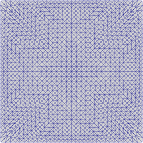
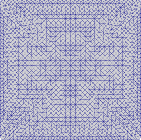
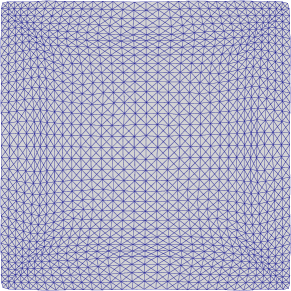
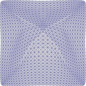
Figure 4: The meshes of $\Omega$ for the final domains produced in the second No PDE experiment in Section 5.1.2: left to right, $p=2,4,\infty$ and second order. Due to symmetry of the result, we show only a half of each mesh. Generally, the first order methods provide a rather good approximation of the expected minimising shape of a square with $p=\infty$ having the most regular triangles around the corners. The Newton method does not quite form the corners we expect.

5.2 A Poisson problem

5.2.1 Poisson experiment 1

For our first experiment we consider $j(x,y)=y$ and $F(x)=2.5(x_{1}+0.5-x_{2}^{2})^{2}+x_{1}^{2}+x_{2}^{2}-1$. This has appeared in [Etl+20, HL21], for example, as a benchmark for the comparisons of shape optimisation algorithms. For the Newton direction we take $t=0.125$. The minimising shape is not explicitly known, however it appears to be a shape not so dissimilar to a kidney. Similarly, the energy of a minimiser is not known.

We start with an approximation of an ellipse with semiaxes $\frac{2}{\sqrt{\pi}}$ and $\frac{1}{\sqrt{\pi}}$ centred at the origin. The triangulation of the domain and hold-all is displayed in Figure 5(a). In Figure 5(b), the energy of shapes along the minimising sequences we produce are given.

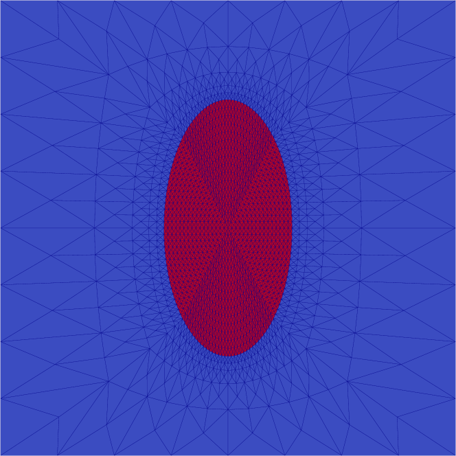
(a) Initial domain for the first Poisson experiment in Section 5.2.1, an approximation of the ellipse with semiaxes $\frac{2}{\sqrt{\pi}}$ and $\frac{1}{\sqrt{\pi}}$ at the origin, is in red and the hold-all, $(-2,2)^{2}$ in blue.

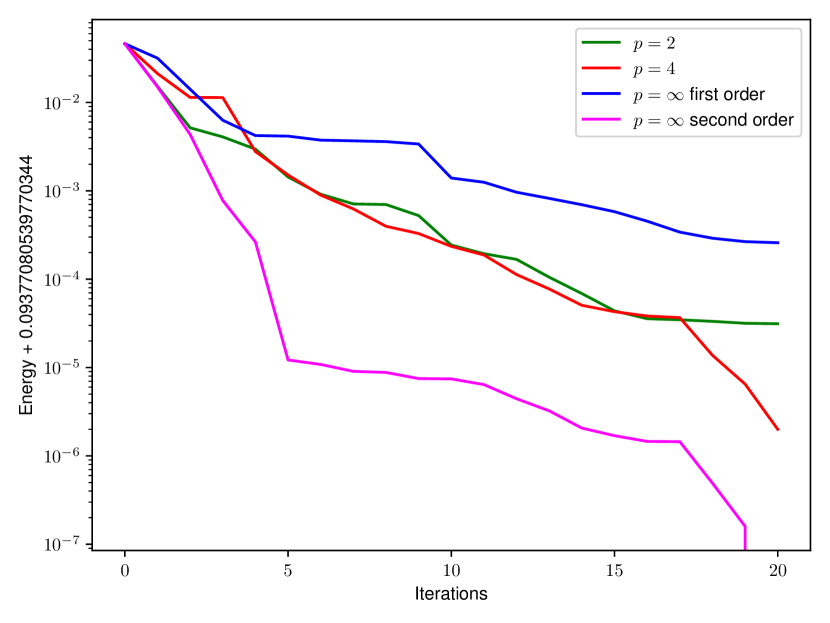
(b) Graph of the energy for the iterates in the first Poisson experiment in Section 5.2.1. We see that $p=\infty$ does not perform as well as the traditional $p=2$ method. The Newton method performs well energetically.

Figure 5: Initial mesh and graph of the energy for the experiment in Section 5.2.1.

In Figure 6, the meshes for the final domains $\Omega$ for each of the methods are given.

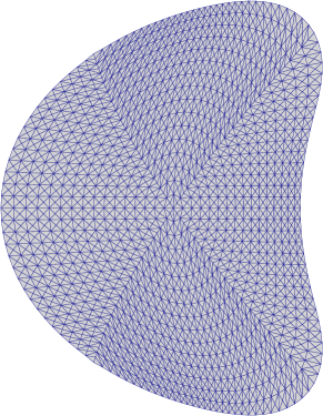
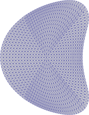
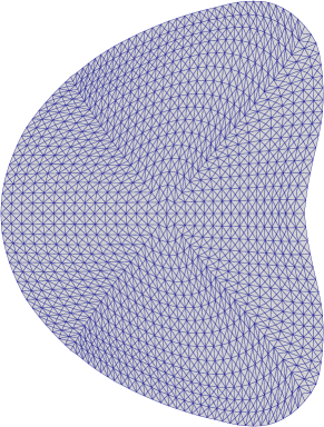
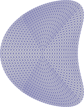
Figure 6: The meshes of $\Omega$ for the final domains produced in the first Poisson experiment in Section 5.2.1: top left to bottom, $p=2,4,\infty$ and second order. Due to symmetry of the result, we show only a half of each mesh. We see that all of the shapes are rather similar, with the $p=\infty$ being a slight outlier. The triangles for both $p=\infty$ and the Newton method appear to be more regularly spaced at the boundary.

5.2.2 Poisson experiment 2

For this experiment we consider $j(x,y)=\frac{1}{2}(y-y_{d}(x))^{2}$ where $y_{d}(x)=\frac{4}{\pi}-|x|^{2}$ and $F=1$. Let us note that $-\Delta y_{d}=4F$. For the Newton direction we take $t=0.125$. This experiment will be equipped with an area constraint that the domain has fixed area $4$ - we will use the same linear constraint on the update direction and projection as in Section 5.1.2. In this setting, we expect the minimiser to be given by the ball of radius $\frac{2}{\sqrt{\pi}}$ at the origin which has energy $\frac{6}{\pi^{2}}$.

We start with the square $(-1,1)^{2}$. The triangulation of the domain and hold-all is displayed in Figure 7(a). In Figure 7(b), the energy of shapes along the minimising sequences we produce are given.

(a) Initial domain for the second Poisson experiment in Section 5.2.2, $(-1,1)^{2}$ is in red and the hold-all, $(-2,2)^{2}$ in blue.

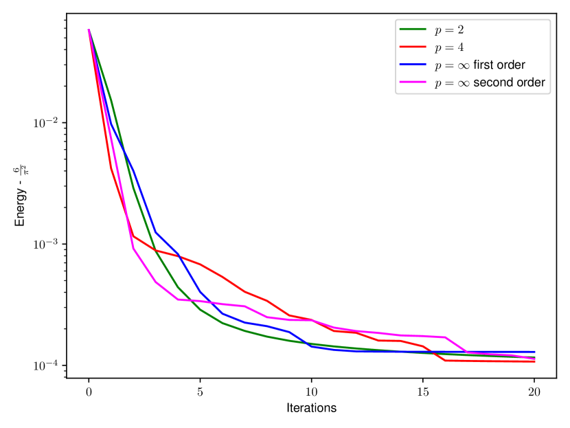
(b) Graph of the energy for the iterates in the second Poisson experiment in Section 5.2.2. We see that all the methods give roughly the same energy.

Figure 7: Initial mesh and graph of the energy for the experiment in Secetion 5.2.2.

In Figure 8, the meshes for the final domains $\Omega$ for each of the methods are given.

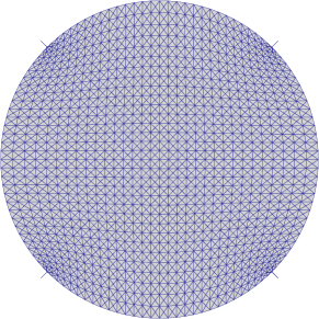
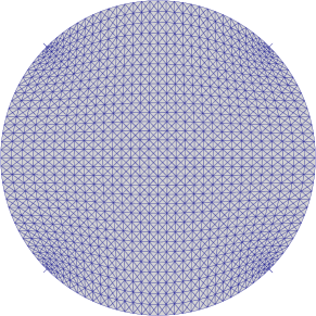
Figure 8: The meshes of $\Omega$ for the final domains produced in the second Poisson experiment in Section 5.2.2: top left to bottom, $p=2,4,\infty$ and second order. Due to symmetry of the result, we show only a quarter of each mesh. We see that both $p=2$ and $p=4$ have very degenerate elements where the corners of the original domain were. Both $p=\infty$ and Newton methods do not have these degenerate triangles. We notice that the triangles which previously made up the corners of the original domain are rather regular in the Newton method. For $p=\infty$, there are many triangles which have obtuse angles.

It is worth noting that when larger values of $t$ were taken during testing, the Newton-type method struggled to perform well. With the Newton method, once the shape was sufficiently close to a ball, the directions generated by ADMM would rotate the almost-ball by large angles which caused large deformations of the mesh in the hold-all.

5.3 A coupled Poisson problem

For this experiment we will consider $j(x,y)=\frac{1}{2}(y_{1}-y_{d}(x))^{2}$ where $y_{d}(x)=0.05+(1-x_{1}^{2})^{3}(1-x_{2}^{2})^{3}$ and $F(x)=\Delta^{2}\left((1-x_{1}^{2})^{3}(1-x_{2}^{2})^{3}\right)$. For the Newton direction we take $t=0.0625$. This experiment will be equipped with an area constraint that the domain has fixed area $4$ - we will use the same linear constraint on the update direction and projection as in Section 5.1.2. One would expect the minimiser to be relatively close to the square $(-1,1)^{2}$ which should have energy $0.005$.

We start with the square $(-1,1)^{2}$. The triangulation of the domain and hold-all is displayed in Figure 9(a). In Figure 9(b), the energy of shapes along the minimising sequences we produce are given.

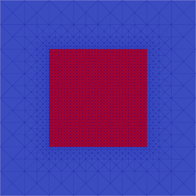
(a) Initial domain for the coupled Poisson experiment in Section 5.3, $(-1,1)^{2}$ is in red and the hold-all, $(-2,2)^{2}$ in blue.

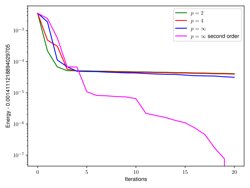
(b) Graph of the energy for the iterates in the coupled Poisson experiment in Section 5.3. We see that $p=\infty$ outperforms the finite $p$ experiments, but the Newton method is energetically performing the best.

Figure 9: Initial mesh and graph of the energy for the experiment in Section 5.3.

In Figure 10, the meshes for the final domains $\Omega$ for each of the methods are given.

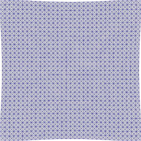
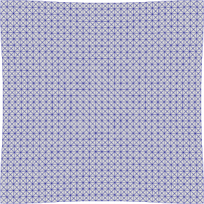
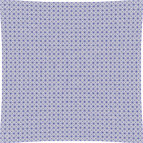
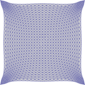
Figure 10: The meshes of $\Omega$ for the final domains produced in the coupled Poisson experiment in Section 5.3: top left to bottom, $p=2,4,\infty$ and second order. Due to symmetry of the result, we show only a quarter of each mesh. To the eye, the first order methods are all seemingly the same. The Newton method appears to have found a more pronounced shape than the others.

5.4 Optimisation of the first eigenvalue for the Laplacian

We use the function eigs from the module sparse.linalg in scipy [Vir+20] to find pairs $(v_{h},\lambda_{h})\in\mathbb{R}^{N_{h}}\times\mathbb{R}$ such that $B_{h}v_{h}=\lambda_{h}M_{h}v_{h}$, where $B_{h}\in\mathbb{R}^{N_{h}\times N_{h}}$ is the stiffness matrix and $M_{h}\in\mathbb{R}^{N_{h}\times N_{h}}$ is the mass matrix. This experiment will be equipped with an area constraint that the domain has fixed area $4$ - we will use the same linear constraint on the update direction and projection as in Section 5.1.2. For the Newton direction we take $t=0.125$. In this setting, the minimiser is known to be the ball of radius $\frac{2}{\sqrt{\pi}}$ which has $\lambda_{1}(B_{\frac{2}{\sqrt{\pi}}})=\beta_{0,1}^{2}\frac{\pi}{4}\approx 4.54210$, where $\beta_{0,1}$ is the first zero of the $0^{th}$ Bessel function.

We start with the square $(-1,1)^{2}$. The triangulation of the domain and hold-all is displayed in Figure 11(a). In Figure 11(b), the energy of shapes along the minimising sequences we produce are given.

(a) Initial domain for the Eigenvalue experiment in Section 5.4, $(-1,1)^{2}$ is in red and the hold-all, $(-2,2)^{2}$ in blue.

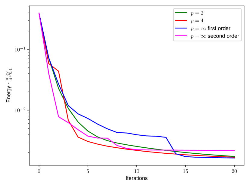
(b) Graph of the energy for the iterates in the Eigenvalue experiment in Section 5.4. We see that all the methods are performing roughly the same.

Figure 11: Initial mesh and graph of the energy for the experiment in Section 5.4.

In Figure 12, the meshes for the final domains $\Omega$ for each of the methods are given.

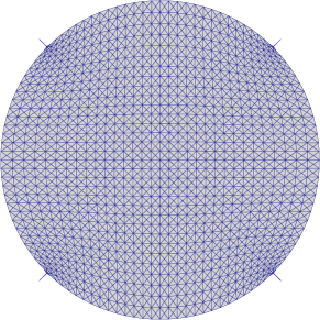
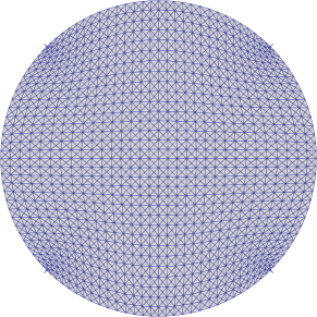
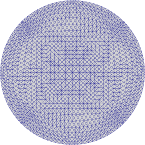
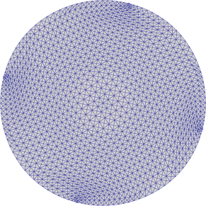
Figure 12: The meshes of $\Omega$ for the final domains produced in the Eigenvalue experiment in Section 5.4: top left to bottom, $p=2,4,\infty$ and second order. Due to symmetry of the result, we show only a quarter of each mesh. We see that spikes appear for $p=2$ and $p=4$ where the corners were for the original shape. The mesh for $p=\infty$ appears rather regular. We comment that the Newton method has lead to the mesh rotating when compared to its original orientation.

Let us further elaborate on Figure 12, particularly the mesh produced by the infinity method. We note that the mesh in the centre for the infinity method appears less regular than the other methods. This appears to occur due to a somewhat undesirable approximation of the shape derivative, which should be concentrated at the boundary. The undesirable approximation is due to the FEM approximation giving interior contributions to the shape derivatives, so-called spurious contributions, in the limit of the mesh becoming infinitely fine this should disappear. Investigation suggests that these are more apparent in the infinity method but disappear when using shape derivatives with only boundary contributions. This sort of expert knowledge is often exploited in the literature and appeared in e.g. [SSW16] to ’delete’ contributions to the shape derivative from nodes on the interior.

Conclusion

In this work we have introduced two new frameworks in which to perform shape optimisation. These methods are more applicable to physical scenarios than the previous works involving $W^{1,\infty}$ as they are not restricted to star-shaped domains. While our examples had star-shaped final domains, our framework allows for more general shapes and is more readily applicable to industrial problems. From the experiments, it was seen that our introduced first order method did not necessarily perform well energetically, however the meshes the method produced are regular. The second order method we introduced performs well both energetically and in terms of the regularity of the mesh, a downside however is the need to tune the damping parameter $t$.

Appendix A Calculations for the second shape derivatives

Here we collect the derivatives of $J$ and $e$ for the examples in Section 5. These derivatives are particularly useful for the calculation of the second shape derivative. All of the maps and functions we consider are sufficiently smooth that we may exchange the order of differentiation. It will be convenient to define

$$\mathbb{D}[V,W]:=\left(\operatorname{div}(V)\operatorname{div}(W)-\operatorname{Tr}(DVDW)\right).$$

A.1 Derivatives for the energy functionals

Let us consider $J$ as in (10), that is $J(V,y):=\int_{\hat{\Omega}}j(\operatorname{id}+V,y)\det(\operatorname{I}+DV)$ for some fixed $\hat{\Omega}\Subset D$. When $j$ is twice differentiable, it holds that

$$J_{V}(0,y)[V]= \int_{\hat{\Omega}}\operatorname{div}Vj(\cdot,y)+j_{x}(\cdot,y)\cdot V,\quad J_{y}(0,y)[\eta]=\int_{\hat{\Omega}}j_{y}(\cdot,y)\,\eta,$$

$$J_{yV}(0,y)[\eta,V]= \int_{\hat{\Omega}}\operatorname{div}Vj_{y}(\cdot,y)\,\eta+j_{yx}(\cdot,y)\cdot V\eta,\quad J_{yy}(0,y)[\eta,\xi]=\int_{\hat{\Omega}}j_{yy}(\cdot,y)\eta\xi,$$

$$J_{VV}(0,y)[V,W]= \int_{\hat{\Omega}}\mathbb{D}[V,W]j(\cdot,y)+\operatorname{div}Vj_{x}(\cdot,y)\cdot W+\operatorname{div}Wj_{x}(\cdot,y)\cdot V+j_{xx}(\cdot,y)V\cdot W.$$

A.2 Derivatives for PDE constraints

Here, we collect the derivatives for the maps $e$ which appear in Sections 5.2, 5.3, and 3.3. Recall that we define $A(V):=(\operatorname{I}+DV)^{-1}(\operatorname{I}+DV)^{-T}$ and $\mathcal{A}[V]:=\operatorname{I}\operatorname{div}V-DV-DV^{T}$. We furthermore define

$$\mathbb{A}[V,W]:= \mathbb{D}[V,W]\operatorname{I}-\operatorname{div}(V)DW-\operatorname{div}(V)DW^{T}$$

$$-\operatorname{div}(W)DV+\left(DWDV+DVDW\right)+DVDW^{T}$$

$$-\operatorname{div}(W)DV^{T}+DWDV^{T}+(DWDV+DVDW)^{T}.$$

A.2.1 Derivatives for the Poisson Problem

In the case that

$$\langle e(V,y),p\rangle=\int_{\hat{\Omega}}\left(A(V)\nabla y\cdot\nabla p-F\circ(\operatorname{id}+V)p\right)\,\det(\operatorname{I}+DV)$$

as in Section 5.2, then it holds that

$$\langle e_{V}(0,y)[V],p\rangle= \int_{\hat{\Omega}}\mathcal{A}[V]\nabla y\cdot\nabla p-\operatorname{div}(VF)p,\quad\langle e_{y}(0,y)[\eta],p\rangle=\int_{\hat{\Omega}}\nabla\eta\cdot\nabla p,$$

$$\langle e_{yV}(0,y)[\eta,V],p\rangle= \int_{\hat{\Omega}}\mathcal{A}[V]\nabla\eta\cdot\nabla p,\quad\langle e_{yy}(0,y)[\eta,\xi],p\rangle=0,$$

$$\langle e_{VV}(0,y)[V,W],p\rangle= \int_{\hat{\Omega}}\mathbb{A}[V,W]\nabla y\cdot\nabla p-\mathbb{D}[V,W]Fp-\operatorname{div}(V)pW\cdot\nabla F$$

$$-\operatorname{div}(W)pV\cdot\nabla F-W\otimes V:pD^{2}F.$$

A.2.2 Derivatives for the coupled Poisson Problem

In the case that

$$\begin{split}\langle e(V,y),p\rangle=&\int_{\hat{\Omega}}\left(A(V)\nabla y_{1}\cdot\nabla p_{2}-y_{2}p_{2}\right)\det(\operatorname{I}+DV)\\ &+\left(A(V)\nabla y_{2}\cdot\nabla p_{1}-p_{1}F\circ(\operatorname{id}+V)\right)\det(\operatorname{I}+DV),\end{split}$$

as in Section 5.3, it holds that

$$\langle e_{V}(0,y)[V],p\rangle= \int_{\hat{\Omega}}\mathcal{A}[V]\nabla y_{1}\cdot\nabla p_{2}-\operatorname{div}Vy_{2}p_{2}+\mathcal{A}[V]\nabla y_{2}\cdot\nabla p_{1}-\operatorname{div}(VF)p_{1},$$

$$\langle e_{y}(0,y)[\eta],p\rangle= \int_{\hat{\Omega}}\nabla\eta_{1}\cdot\nabla p_{2}-\eta_{2}p_{2}+\nabla\eta_{2}\cdot\nabla p_{1},$$

$$\langle e_{yV}(0,y)[\eta,V],p\rangle= \int_{\hat{\Omega}}\mathcal{A}[V]\nabla\eta_{1}\cdot\nabla p_{2}-\operatorname{div}V\eta_{2}p_{1}+\mathcal{A}[V]\nabla\eta_{2}\cdot\nabla p_{2},$$

$$\langle e_{yy}(0,y)[\eta,\xi],p\rangle= 0,$$

$$\langle e_{VV}(0,y)[V,W],p\rangle= \int_{\hat{\Omega}}\mathbb{A}[V,W]\nabla y_{1}\cdot\nabla p_{2}-\mathbb{D}[V,W]y_{2}p_{2}$$

$$+\mathbb{A}[V,W]\nabla y_{2}\cdot\nabla p_{1}-\mathbb{D}[V,W]Fp_{1}$$

$$-\operatorname{div}(V)W\cdot\nabla Fp_{1}-\operatorname{div}(W)V\cdot\nabla Fp_{1}-W\otimes V:D^{2}Fp_{1}.$$

A.2.3 Derivatives for the Eigenvalue Problem

In the case that

$$\begin{split}\langle e(V,(z,\lambda)),(q,\mu)\rangle=&\int_{\hat{\Omega}}\left(A(V)\nabla z\cdot\nabla q-\lambda zq\right)\det(\operatorname{I}+DV)\\ &+\mu\left(1-\int_{\hat{\Omega}}\det(\operatorname{I}+DV)z^{2}\right),\end{split}$$

as in section 3.3, it holds that

$$\langle e_{V}(0,(z,\lambda))[V],(q,\mu)\rangle= \int_{\hat{\Omega}}\mathcal{A}[V]\nabla z\cdot\nabla q-\lambda\operatorname{div}Vzq-\mu\operatorname{div}Vz^{2},$$

$$\langle e_{y}(0,(z,\lambda))[(\eta,\tilde{\eta})],(q,\mu)\rangle= \int_{\hat{\Omega}}\nabla\eta\cdot\nabla q-\lambda\eta q-\tilde{\eta}zq-\mu z\eta,$$

$$\langle e_{Vy}(0,(z,\lambda))[V,(\eta,\tilde{\eta})],(q,\mu)\rangle= \int_{\hat{\Omega}}\mathcal{A}[V]\nabla q\cdot\nabla\eta-\operatorname{div}V\lambda\eta q-\operatorname{div}V\tilde{\eta}zq$$

$$-2\mu\int_{\hat{\Omega}}\operatorname{div}Vz\eta,$$

$$\langle e_{yy}(0,(z,\lambda))[(\eta,\tilde{\eta}),(\zeta,\tilde{\zeta)}],(q,\mu)\rangle= \int_{\hat{\Omega}}-\tilde{\zeta}\eta q-\tilde{\eta}\zeta q-\mu\zeta\eta,$$

$$\langle e_{VV}(0,(z,\lambda))[V,W],(q,\mu)\rangle= \int_{\hat{\Omega}}\mathbb{A}[V,W]\nabla z\cdot\nabla q-\mathbb{D}[V,W]\left(\lambda zq-\mu z^{2}\right).$$

For the energy, $J(V,(z,\lambda))=\lambda$, it is clear that only the derivative in the second component is non-vanishing and one has that

$$J_{y}(0,(z,\lambda)[(\eta,\tilde{\eta})]= \tilde{\eta}.$$

References

- [ADJ21] Grégoire Allaire, Charles Dapogny and François Jouve “Shape and topology optimization” In Differential Geometric Partial Differential Equations: Part II 22, Handbook of Numerical Analysis Amsterdam, Netherlands: Elsevier, 2021, pp. 3–124
- [BM20] S. Bartels and M. Milicevic “Efficient iterative solution of finite element discretized nonsmooth minimization problems” In Comput. Math. Appl. 80.5, 2020, pp. 588–603 DOI: 10.1016/j.camwa.2020.04.026
- [Bar21] Sören Bartels “Nonconforming discretizations of convex minimization problems and precise relations to mixed methods” In Computers & Mathematics with Applications 93, 2021, pp. 214–229 DOI: https://doi.org/10.1016/j.camwa.2021.04.014
- [Bas+21] Peter Bastian et al. “The Dune framework: Basic concepts and recent developments” Development and Application of Open-source Software for Problems with Numerical PDEs In Computers & Mathematics with Applications 81, 2021, pp. 75–112 DOI: https://doi.org/10.1016/j.camwa.2020.06.007
- [Bel+97] Juan Antonio Bello, Enrique Fernández-Cara, Jérôme Lemoine and Jacques Simon “The Differentiability of the Drag with Respect to the Variations of a Lipschitz Domain in a Navier–Stokes Flow” In SIAM Journal on Control and Optimization 35.2, 1997, pp. 626–640 DOI: 10.1137/S0363012994278213
- [Ben+15] Jean-David Benamou et al. “Iterative Bregman Projections for Regularized Transportation Problems” In SIAM Journal on Scientific Computing 37.2, 2015, pp. A1111–A1138 DOI: 10.1137/141000439
- [BCS21] A. Boulkhemair, A. Chakib and A Sadik “On a shape derivative formula for a family of star-shaped domains” In HAL preprint, hal-02084874, 2021 URL: https://hal.archives-ouvertes.fr/hal-02084874
- [DHH22] Klaus Deckelnick, Philip J. Herbert and Michael Hinze “A novel approach to shape optimisation with Lipschitz domains” In ESAIM: COCV 28, 2022, pp. 2 DOI: 10.1051/cocv/2021108
- [DHH23] Klaus Deckelnick, Philip J. Herbert and Michael Hinze “Convergence of a steepest descent algorithm in shape optimisation using functions” In arXiv preprint arXiv:2310.15078, 2023
- [DN18] Andreas Dedner and Martin Nolte “The Dune Python Module” In arXiv preprint 1807.05252, 2018 ARXIV ̵PREPRINT ̵ARXIV:1807.05252: 1807.05252
- [DNK20] Andreas Dedner, Martin Nolte and Robert Klöfkorn “Python Bindings for the DUNE-FEM module” Zenodoo, 2020 DOI: 10.5281/zenodo.3706994
- [DZ11] M.C. Delfour and J.P. Zolesio “Shapes and Geometries: Metrics, Analysis, Differential Calculus, and Optimization, Second Edition”, Advances in Design and Control Society for IndustrialApplied Mathematics (SIAM, 3600 Market Street, Floor 6, Philadelphia, PA 19104), 2011 URL: https://books.google.co.uk/books?id=fjjvX9a9cxUC
- [ES18] Martin Eigel and Kevin Sturm “Reproducing kernel Hilbert spaces and variable metric algorithms in PDE-constrained shape optimization” In Optimization Methods and Software 33.2 Taylor & Francis, 2018, pp. 268–296
- [EH22] Charles M Elliott and Philip J Herbert “A formula for membrane mediated point particle interactions on near spherical biomembranes” In Interfaces and Free Boundaries 24.1, 2022, pp. 1–34
- [EHS07] Karsten Eppler, Helmut Harbrecht and Reinhold Schneider “On convergence in elliptic shape optimization” In SIAM Journal on Control and Optimization 46.1 SIAM, 2007, pp. 61–83
- [Etl+20] Tommy Etling, Roland Herzog, Estefanı́a Loayza and Gerd Wachsmuth “First and Second Order Shape Optimization Based on Restricted Mesh Deformations” In SIAM Journal on Scientific Computing 42.2, 2020, pp. A1200–A1225 DOI: 10.1137/19M1241465
- [Fis+17] Michael Fischer, Florian Lindemann, Michael Ulbrich and Stefan Ulbrich “Fréchet Differentiability of Unsteady Incompressible Navier–Stokes Flow with Respect to Domain Variations of Low Regularity by Using a General Analytical Framework” In SIAM Journal on Control and Optimization 55.5 SIAM, 2017, pp. 3226–3257
- [Gar+15] H. Garcke, C. Hecht, M. Hinze and C. Kahle “Numerical approximation of phase field based shape and topology optimization for fluids” In SIAM J. Sci. Comput. 37, 2015, pp. A1846–A1871
- [Gar+18] H. Garcke, M. Hinze, C. Kahle and K.F. Lam “A phase field approach to shape optimization in Navier- Stokes flow with integral state constraints” In Adv. Comput. Math. 44, 2018, pp. 1345–1383
- [Gil+77] David Gilbarg, Neil S Trudinger, David Gilbarg and NS Trudinger “Elliptic partial differential equations of second order” Springer, 1977
- [GM94] Ph Guillaume and M Masmoudi “Computation of high order derivatives in optimal shape design” In Numerische Mathematik 67.2 Springer, 1994, pp. 231–250
- [HSU21] J Haubner, Martin Siebenborn and Michael Ulbrich “A continuous perspective on shape optimization via domain transformations” In SIAM Journal on Scientific Computing 43.3 SIAM, 2021, pp. A1997–A2018
- [HUU20] Johannes Haubner, Michael Ulbrich and Stefan Ulbrich “Analysis of shape optimization problems for unsteady fluid-structure interaction” In Inverse Problems 36, 2020, pp. 1–38
- [HY15] Bingsheng He and Xiaoming Yuan “On non-ergodic convergence rate of Douglas–Rachford alternating direction method of multipliers” In Numerische Mathematik 130, 2015 DOI: 10.1007/s00211-014-0673-6
- [Hen06] Antoine Henrot “Extremum problems for eigenvalues of elliptic operators” Springer Science & Business Media, 2006
- [HP18] Antoine Henrot and Michel Pierre “Shape Variation and Optimization: A Geometrical Analysis”, EMS tracts in mathematics European Mathematical Society, 2018 URL: https://books.google.co.uk/books?id=%5C_fCqswEACAAJ
- [Her23] Philip J. Herbert “Shape Optimisation in : A connection between the steepest descent and Optimal Transport” In arXiv preprint arXiv:2301.07994, 2023
- [HL21] Roland Herzog and Estefanı́a Loayza-Romero “A Discretize-Then-Optimize Approach to PDE-Constrained Shape Optimization” In arXiv preprint arXiv:2109.00076, 2021
- [Hin+08] Michael Hinze, René Pinnau, Michael Ulbrich and Stefan Ulbrich “Optimization with PDE constraints” Springer Science & Business Media, 2008
- [HPS15] Ralf Hiptmair, Alberto Paganini and Sahar Sargheini “Comparison of approximate shape gradients” In BIT Numerical Mathematics 55.2 Springer, 2015, pp. 459–485
- [ISW18] José A Iglesias, Kevin Sturm and Florian Wechsung “Two-dimensional shape optimization with nearly conformal transformations” In SIAM Journal on Scientific Computing 40.6 SIAM, 2018, pp. A3807–A3830
- [Küh+19] N. Kühl, P.M. Müller, M. Hinze and T. Rung “Decoupling of Control and Force Objective in Adjoint-Based Fluid Dynamic Shape Optimization” In AIAA Journal 57, 2019, pp. 4110
- [Las17] Monika Laskawy “Optimality conditions of the first eigenvalue of a fourth order Steklov problem” In Communications on Pure and Applied Analysis 16.5, 2017, pp. 1843–1859 DOI: 10.3934/cpaa.2017089
- [LS21] Daniel Luft and Volker Schulz “Pre-shape calculus and its application to mesh quality optimization” In Control and Cybernetics 50.3, 2021, pp. 263–301 DOI: doi:10.2478/candc-2021-0019
- [LS21a] Daniel Luft and Volker Schulz “Simultaneous shape and mesh quality optimization using pre-shape calculus.” In Control & Cybernetics 50.4, 2021
- [Mül+21] Peter Marvin Müller et al. “A Novel -Harmonic Descent Approach Applied to Fluid Dynamic Shape Optimization” In Structural and Multidisciplinary Optimization, 2021
- [Mül+22] Peter Marvin Müller, Jose Pinzon, Thomas Rung and Martin Siebenborn “A Scalable Algorithm for Shape Optimization with Geometric Constraints in Banach Spaces” In arXiv preprint arXiv:2205.01912, 2022
- [MS76] François Murat and Jacques Simon “Etude de problemes d’optimal design” In Optimization Techniques Modeling and Optimization in the Service of Man Part 2 Berlin, Heidelberg: Springer Berlin Heidelberg, 1976, pp. 54–62
- [OS21] Sofiya Onyshkevych and Martin Siebenborn “Mesh quality preserving shape optimization using nonlinear extension operators” In Journal of Optimization Theory and Applications 189.1 Springer, 2021, pp. 291–316
- [PWF18] Alberto Paganini, Florian Wechsung and Patrick E Farrell “Higher-order moving mesh methods for PDE-constrained shape optimization” In SIAM Journal on Scientific Computing 40.4 SIAM, 2018, pp. A2356–A2382
- [Pir74] O. Pironneau “On optimum design in fluid mechanics” In Journal of Fluid Mechanics 64.1 Cambridge University Press, 1974, pp. 97–110 DOI: 10.1017/S0022112074002023
- [RCP16] Antoine Rolet, Marco Cuturi and Gabriel Peyré “Fast dictionary learning with a smoothed Wasserstein loss” In Artificial Intelligence and Statistics, 2016, pp. 630–638 PMLR
- [Sch+13] S. Schmidt, C. Ilic, V. Schulz and N. Gauger “Three dimensional large scale aerodynamic shape optimization based on the shape calculus” In AIAA Journal 51, 2013, pp. 2615–2627
- [SS23] Stephan Schmidt and Volker H. Schulz “A Linear View on Shape Optimization” In SIAM Journal on Control and Optimization 61.4, 2023, pp. 2358–2378 DOI: 10.1137/22M1488910
- [SSW15] Volker Schulz, Martin Siebenborn and Katrin Welker “PDE constrained shape optimization as optimization on shape manifolds” In Geometric Science of Information 9389, Lecture Notes in Computer Science New York: Springer, 2015, pp. 499–508
- [SSW16] Volker Schulz, Martin Siebenborn and Katrin Welker “Efficient PDE constrained shape optimization based on Steklov-Poincaré type metrics” In Siam J. Optim. 26, 2016, pp. 2800–2819
- [SW17] M. Siebenborn and K. Welker “Algorithmic Aspects of Multigrid Methods for Optimization in Shape Spaces” In Siam J. Sci. Comput. 39.6, 2017, pp. B1156–B1177
- [Sim80] Jacques Simon “Differentiation with respect to the domain in boundary value problems” In Numerical Functional Analysis and Optimization 2.7-8 Taylor & Francis, 1980, pp. 649–687
- [Vir+20] Pauli Virtanen et al. “SciPy 1.0: Fundamental Algorithms for Scientific Computing in Python” In Nature Methods 17, 2020, pp. 261–272 DOI: 10.1038/s41592-019-0686-2