State-constrained Optimization Problems under Uncertainty: A Tensor Train Approach

Abstract.

We propose an algorithm to solve optimization problems constrained by partial (ordinary) differential equations under uncertainty, with almost sure constraints on the state variable. To alleviate the computational burden of high-dimensional random variables, we approximate all random fields by the tensor-train decomposition. To enable efficient tensor-train approximation of the state constraints, the latter are handled using the Moreau-Yosida penalty, with an additional smoothing of the positive part (plus/ReLU) function by a softplus function. We derive theoretical bounds on the constraint violation in terms of the Moreau-Yosida regularization parameter and smoothing width of the softplus function. This result also proposes a practical recipe for selecting these two parameters. When the optimization problem is strongly convex, we establish strong convergence of the regularized solution to the optimal control. We develop a second order Newton type method with a fast matrix-free action of the approximate Hessian to solve the smoothed Moreau-Yosida problem. This algorithm is tested on benchmark elliptic problems with random coefficients, optimization problems constrained by random elliptic variational inequalities, and a real-world epidemiological model with 20 random variables. These examples demonstrate mild (at most polynomial) scaling with respect to the dimension and regularization parameters.

1. Introduction

Over last two decades optimization problems constrained by physical laws, such as partial (ordinary) differential equations (PDEs/ODEs), have emerged as a prominent research area. This is fueled by many applications in science and engineering, such as controlling pathogen propagation in built environment [26, 25], shape and topology optimization [36, 28], optimal strategies to predict shutdowns due to pandemics [11]. The optimization variables consist of state $(y)$ and control/design $(u)$. However, often due to noisy measurements and ambiguous models due to incomplete physics, the underlying physical laws contain uncertainty. This has led to significant theoretical and algorithmic developments in the area of optimization problems constrained by physical laws under uncertainty. See for instance [23, 4, 14, 3] and the references therein. These papers focus on problems with control constraints.

The literature on state-constrained optimization problems under uncertainty is scarce. For instance, [12, 17] use probability constraints, and [15, 13, 16] consider almost surely type constraints. It is well-known that even in the deterministic setting, the state constrained problems are highly challenging. One of the fundamental difficulties is that the state constraints are imposed in the sense of continuous functions. As a result, the Lagrange multipliers corresponding to those constraints are Radon measures that exhibit low regularity [6]. The situation is much more delicate in the stochastic setting. We refer to the aforementioned references for a detailed discussion on this topic. Motivated by the deterministic setting, [13] introduces a Moreau-Yosida based approximation scheme to solve the state-constrained optimization problems when the PDE constraints are given by an elliptic equation with random coefficients. Further extensions of this work are considered in [1, 16]. However, all of these papers approximate expectations of random fields by Monte-Carlo-type methods, which may converge slowly.

In [3], we introduced an algorithm (TTRISK) based on the tensor train (TT) decomposition [30] to solve risk-averse optimization problems with control constraints, and the conditional value-at-risk (CVaR) [32] risk measure. We demonstrated that the extra computational cost due to the uncertainty can scale proportionally to $\mathrm{error}^{-0.5}$ when the TT approximation is used, in contrast to a $\mathrm{error}^{-2}$ scaling of Monte Carlo quadratures. In the current paper, we continue this program and develop a TT based algorithm for state-constrained optimization problems. For simplicity of presentation, we only consider the risk-neutral setting, i.e., the objective function is given by the expected value of a quantity of interest. Similarly to [13, 16], we tackle the state constrains using Moreau-Yosida based relaxation with a softplus smoothing. The main contributions of this paper are listed next:

1. We consider an $\varepsilon$-softplus regularization of the positive part function $(\cdot)_{+}=\max\{\cdot,0\}$ and derive a probabilistic estimate of state constraint violation in terms of Moreau-Yosida regularization parameter $\gamma$ and $\varepsilon$. In particular, we show that selecting $\varepsilon\propto\gamma^{-1/2}$ ensures the convergence of the constraint violation with a rate $\gamma^{-1/2}$. This result is motivated by [13, Prop. 2]. Notice that the $\varepsilon$-smoothing is carried out because the irregular function $(\cdot)_{+}$ may lack an efficient TT decomposition.

2. When the optimization problem is strongly convex, we establish strong convergence of the regularized solution to the optimal control. Our final results can be seen as generalizations of the results in deterministic setting.

3. We derive a second order Newton type method to solve the regularized problem with a fast matrix-free action of the approximate Hessian.

4. We test the proposed method on elliptic equations in one and two physical dimensions and random coefficients, as well as an ODE example (motivated by a realistic application) with 20 random variables, and show that the algorithm is free from the curse of dimensionality.

5. The proposed approach has been also successfully applied to an example where the PDE constraint is given by an elliptic variational inequality.

Outline: The remainder of the paper is organized as follows. In Section 2, we provide a rigorous mathematical formulation of the problem under consideration. Section 3 is devoted to the Moreau-Yosida approximation, derivation of the second order Newton method and approximation error estimates due to the Moreau-Yosida approximation. In Section 4, we provide a brief description of the TT format. This is followed by practical aspects of Moreau-Yosida approximations in Section 5. Finally, in Section 6, we provide a series of numerical experiments. At first, we consider an optimization problem with an elliptic PDE in one spatial dimension as constraints. This is followed by a two-dimensional case. After these benchmarks, an optimization problem with an elliptic variational inequality as constraint is considered in Section 6.3. The numerical experiments conclude with a realistic ODE example for designing optimal lockdown strategies in Section 6.4.

2. Problem Formulation

Let $(\Omega,\mathcal{F},\mathbb{P})$ denote a complete probability space, where $\Omega$ represents the sample space, $\mathcal{F}$ is the Borel $\sigma$-algebra of events on the power set of $\Omega$, and $\mathbb{P}\mathrel{\mathop{\mathchar 58\relax}}\Omega\rightarrow[0,1]$ is an appropriate probability measure. We denote by $\mathbb{E}[\cdot]$ the expectation with respect to $\mathbb{P}$. Let $\mathcal{U}$ be a real deterministic reflexive Banach space of optimization variables (control or design) defined on an open, bounded and connected set $D\subset\mathbb{R}^{n}$ with Lipschitz boundary. We denote by $\|\cdot\|_{\mathcal{U}}$ the norm on $\mathcal{U}$, and the duality pairing between $\mathcal{U}$ and $\mathcal{U}^{*}$ as $\langle\cdot,\cdot\rangle_{\mathcal{U}^{*},\mathcal{U}}$. Let $\mathcal{Y}=L^{2}(\Omega,\mathcal{F},\mathbb{P};\mathcal{\hat{Y}})$ and $\mathcal{Z}=L^{2}(\Omega,\mathcal{F},\mathbb{P};\mathcal{\hat{Z}})$ be Bochner spaces of random fields, based on deterministic Banach spaces $\mathcal{\hat{Y}}\hookrightarrow L^{2}(D)\hookrightarrow\mathcal{\hat{Y}}^{*}$ and $\mathcal{\hat{Z}}$, with corresponding norms and duality pairings

$$\|y\|_{\mathcal{Y}}^{2}=\mathbb{E}[\|y(\omega)\|_{\mathcal{\hat{Y}}}^{2}],\qquad\langle y,v\rangle_{\mathcal{Y}^{*},\mathcal{Y}}=\mathbb{E}\left[\langle y(\omega),v(\omega)\rangle_{\mathcal{\hat{Y}}^{*},\mathcal{\hat{Y}}}\right],$$

and similarly for $\mathcal{Z}$. Let $\mathcal{U}_{ad}\subseteq\mathcal{U}$ be a closed convex nonempty subset and let $c\mathrel{\mathop{\mathchar 58\relax}}\mathcal{Y}\times\mathcal{U}_{ad}\times\Omega\rightarrow\mathcal{Z}$ denote, e.g., a partial differential operator, then consider the equality constraint

$$c(y,u;\omega)=0,\quad\mbox{in }\mathcal{Z},\quad\mbox{a.s. }\omega\in\Omega,$$

where a.s. indicates “almost surely” with respect to the probability measure $\mathbb{P}$.

In this paper, we consider the optimization problems of the form

$$\min_{y,u}\mathcal{R}[J(y,u;\omega)]$$ (2.1)

$$\mbox{s.t}\;\;\;c(y,u;\omega) = 0,\quad\mbox{in}\;\mathcal{Z},\quad\mbox{a.s. }\omega\in\Omega,$$ (2.2)

where $\mathcal{R}$ represents the risk measure and $\mathcal{R}[J(y,u;\omega)]$ is a deterministic cost function. More precisely, we will focus on the so-called risk-neutral formulation; that is, $\mathcal{R}$ is simply the expectation, denoted by $\mathbb{E}$. We are particularly interested in the case in which the state variable $y$ is constrained by a random variable:

$$y\leq y_{\max}(\omega)\quad\mbox{a.s.},$$ (2.3)

where we assume that $y_{\max}\in\mathcal{Y}$.

In what follows, we discuss the Moreau-Yosida approximation for (2.1)-(2.3) and derive a Newton type method. Throughout the paper, without explicitly stating, we will make use of the following assumption.

Assumption 2.1 (unique forward solution).

There exists an injective operator $S(\omega)\mathrel{\mathop{\mathchar 58\relax}}\mathcal{U}_{ad}\rightarrow\mathcal{Y}$ (maybe nonlinear) such that $c(S(\omega)u,u;\omega)=0$ $\forall u\in\mathcal{U}_{ad}$ a.s.

This allows us to define the reduced-space cost function

$$j(u)\mathrel{\mathop{\mathchar 58\relax}}=\mathcal{R}[J(S(\omega)u,u;\omega)].$$ (2.4)

The resulting reduced optimization problem is given by

$$\begin{aligned} &\min_{u\in\mathcal{U}_{ad}}j(u)\\ &\mbox{s.t}\;\;\;y\leq y_{\max}(\omega)\quad\mbox{a.s.}\end{aligned}$$ (2.5)

3. Smoothed Moreau-Yosida approximation

Solving (2.5) with state constraints involve computation of the indicator function of an active set and/or Lagrange multiplier as a random field that is nonnegative on a complicated high-dimensional domain. This may be difficult for many function approximation methods, especially for tensor decompositions that are considered in this paper. We tackle this difficulty by first turning the constrained optimization problem (2.5) into an unconstrained optimization problem with the Moreau-Yosida penalty, and further by smoothing the indicator function in the penalty term.

The classical Moreau-Yosida problem reads, with $\gamma\geq 0$ denoting the regularization parameter,

$$\min_{u\in\mathcal{U}_{ad}}j^{\gamma}(u),\quad\mbox{where}\quad j^{\gamma}(u)\mathrel{\mathop{\mathchar 58\relax}}=j(u)+\frac{\gamma}{2}\mathbb{E}\left[\left\|(Su-y_{\max}(\xi))_{+}\right\|^{2}_{L^{2}(D)}\right],$$ (3.1)

where the so-called positive part or ReLU function $(\cdot)_{+}$ reads $(s)_{+}=s$ if $s\geq 0$ and $0,$ otherwise. Here, we have removed the need to optimize the Lagrange multiplier (corresponding to the inequality constraints) over the nonnegative cone, but the function approximation of a nonsmooth high-dimensional random field $(Su-y_{\max}(\xi))_{+}$ (and derivatives thereof) may be still inefficient.

For this reason, we replace the ReLU function in the penalty term by a smoothed version. In this paper, we use the softplus function

$$g_{\varepsilon}(s)=\varepsilon\cdot\log(1+\exp(s/\varepsilon))\in C^{\infty}(\mathbb{R}),\qquad g_{0}(s)=\lim_{\varepsilon\rightarrow 0}g_{\varepsilon}(x)=(s)_{+},$$ (3.2)

although other (e.g. piecewise polynomial) functions are also possible [24, 1]. Now, the cost function becomes

$$j^{\gamma,\varepsilon}(u)\mathrel{\mathop{\mathchar 58\relax}}=j(u)+\frac{\gamma}{2}\mathbb{E}\left[\left\|g_{\varepsilon}(Su-y_{\max})\right\|^{2}_{L^{2}(D)}\right].$$ (3.3)

3.1. Discretization and Derivatives of the Cost

In practice, the operator $S$ involves the solution of a differential equation, which needs to be discretized (using e.g. Finite Element methods and/or time integration schemes). For a given mesh parameter $h>0$, we introduce the discretized (maybe nonlinear) operator $\mathbf{S}_{h}(\omega)\mathrel{\mathop{\mathchar 58\relax}}\mathcal{U}_{ad}\rightarrow\mathbb{R}^{n_{y}}$, where $n_{y}$ is the total number of degrees of freedom in the discrete solution. We denote the induced Bochner space $\mathcal{Y}_{h}\cong L^{2}_{h}(\Omega,D)\mathrel{\mathop{\mathchar 58\relax}}=L^{2}(\Omega,\mathcal{F},\mathbb{P};\mathbb{R}^{n_{y}})$. The $L^{2}$-norm can be written as an expectation of a vector quadratic form,

$$\|\mathbf{y}\|^{2}_{L^{2}_{h}(\Omega,D)}=\mathbb{E}\left[\mathbf{y}(\omega)^{\top}\mathbf{M}\mathbf{y}(\omega)\right],\qquad\forall\mathbf{y}\in L^{2}_{h}(\Omega,D),$$

where $\mathbf{M}=\mathbf{M}^{\top}>0\in\mathbb{R}^{n_{y}\times n_{y}}$ is a mass matrix. The discretized problem cost is denoted by $j^{h}(u)\approx j(u)$, and the discretized constraint is $\mathbf{y}_{\max}^{h}\in\mathcal{Y}_{h}$. Now, the semi-discretized Moreau-Yosida cost function (3.3) becomes

$$j^{\gamma,\varepsilon,h}(u)\mathrel{\mathop{\mathchar 58\relax}}=j^{h}(u)+\frac{\gamma}{2}\mathbb{E}\left[\|g_{\varepsilon}(\mathbf{S}_{h}u-\mathbf{y}_{\max}^{h})\|_{\mathbf{M}}^{2}\right].$$ (3.4)

To derive a Newton type method, we compute the expressions of gradient and Hessian:

$$\nabla_{u}j^{\gamma,\varepsilon,h} =\nabla_{u}j^{h}+\gamma\mathbb{E}\left[\mathbf{S}_{h}^{*}\cdot\mathrm{diag}(g^{\prime}_{\varepsilon}(\mathbf{S}_{h}u-\mathbf{y}_{\max}^{h}))\cdot\mathbf{M}g_{\varepsilon}(\mathbf{S}_{h}u-\mathbf{y}_{\max}^{h})\right],$$ (3.5)

$$\nabla_{uu}j^{\gamma,\varepsilon,h} =\nabla^{2}_{uu}j^{h}+\gamma\mathbb{E}\left[\mathbf{S}_{h}^{*}\cdot\mathrm{diag}(g^{\prime}_{\varepsilon})\mathbf{M}\mathrm{diag}(g^{\prime}_{\varepsilon})\cdot\mathbf{S}_{h}^{\prime}\right]$$ (3.6)

$$+\gamma\mathbb{E}\left[\mathbf{S}_{h}^{*}\cdot(\mathrm{tendiag}(g^{\prime\prime}_{\varepsilon})\times_{3}(\mathbf{M}g_{\varepsilon}))\cdot\mathbf{S}_{h}^{\prime}\right]$$ (3.7)

$$+\gamma\mathbb{E}\left[\nabla_{u}\mathbf{S}_{h}^{*}\times_{3}(\mathrm{diag}(g^{\prime}_{\varepsilon}(\mathbf{S}_{h}u-\mathbf{y}_{\max}^{h}))\cdot\mathbf{M}g_{\varepsilon}(\mathbf{S}_{h}u-\mathbf{y}_{\max}^{h}))\right],$$ (3.8)

where $\mathrm{tendiag}(\cdot)$ is producing a $3$-dimensional tensor out of vector by putting the vector elements along the diagonal, and zero elements otherwise, and $\times_{3}$ is the tensor-vector contraction product over the $3$d mode of the tensor. If $\mathbf{S}_{h}$ is a nonlinear operator, $\mathbf{S}_{h}^{\prime}=\nabla_{u}\mathbf{S}_{h}(u)$ denotes the gradient of an image of $u$, and $\mathbf{S}_{h}^{*}$ is the adjoint of $\mathbf{S}_{h}^{\prime}$.

3.2. Matrix-free Fixed Point Gauss-Newton Hessian

The exact assembly of all terms of the Hessian (3.6)–(3.8) can be too computationally expensive, since this involves dense tensor-valued random fields (such as $\nabla_{u}\mathbf{S}_{h}^{*}$). To simplify the computations, we can firstly omit the terms (3.7) and (3.8) which contain order-3 tensors. Secondly, we can replace the exact expectation by a fixed-point evaluation. Rewriting (2.1) using Assumption 2.1 we can define $J(u;\omega)=J(S(\omega)u,u;\omega)$ and its discretized version $J^{h}(u;\omega)=J(\mathbf{S}_{h}(\omega)u,u;\omega)$. The Hessian of $j^{h}$ can then be written as

$$\nabla_{uu}^{2}j^{h}=\mathbb{E}\left[\nabla_{uu}^{2}J^{h}(u;\omega)\right].$$

For practical computations, it is convenient to parametrize all random fields with independent identically distributed (i.i.d.) random variables with a known probability density function. Those variables can then be sampled independently, and an expectation can be computed simply by quadrature. Therefore, we will use the following assumption.

Assumption 3.1 (finite noise).

There exists a $d$-dimensional random vector $\xi(\omega)\in\mathbb{R}^{d}$ with a product probability density function $\pi(\xi)=\pi(\xi_{1})\cdots\pi(\xi_{d}),$ such that any random field $y\in\mathcal{Y}$ can be expressed as a function of $\xi$, $y(\omega)=y(\xi(\omega))$ a.s., and

$$\mathbb{E}[y]=\int_{\mathbb{R}^{d}}y(\xi)\pi(\xi)d\xi.$$

In particular, the vector $\xi$ can often be derived from a parametrization of the forward solution operator $\mathbf{S}_{h}(\omega)=\mathbf{S}_{h}(\xi(\omega))$, and/or the constraint $\mathbf{y}_{\max}^{h}(\omega)=\mathbf{y}_{\max}^{h}(\xi(\omega))$.

Example 3.2.

Let $y=S(\nu(\omega))u$ be the resolution of an elliptic PDE

$$-\nabla(\kappa(x;\nu(\omega))\nabla y)=u,$$

where the diffusivity

$$\kappa(x;\nu(\omega))=\kappa_{0}(x)+\sum_{k=1}^{p}\psi_{k}(x)\nu_{k}(\omega)$$

and the constraint

$$y_{\max}(x;\eta(\omega))=y_{0}(x)+\sum_{k=1}^{q}\phi_{k}(x)\eta_{k}(\omega)$$

are given by Karhunen-Loeve expansions (see e.g., [27]), where $\nu$ and $\eta$ are independent random variables. Then, we can define $\xi=(\nu_{1},\ldots,\nu_{p},\eta_{1},\ldots,\eta_{q})$.

Now we can replace $\nabla_{uu}^{2}j^{h}=\mathbb{E}[\nabla_{uu}^{2}J^{h}(u;\xi)]$ by

$$\tilde{\nabla}_{uu}^{2}j^{h}=\nabla_{uu}^{2}J^{h}(u;\mathbb{E}[\xi]).$$

This is exact if $\nabla_{uu}^{2}J^{h}$ is linear in $\xi$, but we can take it as an approximation in the general case too. Now to apply $\tilde{\nabla}_{uu}^{2}j^{h}$ to a vector we just need to apply one deterministic $\nabla_{uu}^{2}J^{h}(u;\mathbb{E}[\xi])$, which involves solving one forward, one adjoint, and two linear sensitivity (of state and adjoint) deterministic problems in the most general setting [4, Ch. 1, Algo. 2].

Similarly we approximate the second term in (3.6) by

$$\gamma\mathbf{S}_{h}^{*}(\xi_{*})\mathbf{M}\mathbf{S}_{h}^{\prime}(\xi_{*}),$$

where

$$\xi_{*}=\frac{\mathbb{E}\left[\xi\cdot\mathbf{1}^{\top}g^{\prime}_{\varepsilon}(\mathbf{S}_{h}u-\mathbf{y}_{\max}^{h}(\xi))\right]}{\mathbb{E}\left[\mathbf{1}^{\top}g^{\prime}_{\varepsilon}(\mathbf{S}_{h}u-\mathbf{y}_{\max}^{h}(\xi))\right]}$$

is the mean of the random variable with respect to the probability density $\pi_{g^{\prime}}\propto\pi\cdot(\mathbf{1}^{\top}g^{\prime}_{\varepsilon}(\mathbf{S}_{h}u-\mathbf{y}_{\max}^{h}))$, and $\mathbf{1}\in\mathbb{R}^{n_{y}}$ is the constant vector, averaging the spatial components. Note that $\mathbf{1}^{\top}g^{\prime}_{\varepsilon}(\mathbf{S}_{h}u-\mathbf{y}_{\max}^{h})$ is a nonnegative function bounded by $n_{y}$, so $\pi\mathbf{1}^{\top}g^{\prime}_{\varepsilon}(\mathbf{S}_{h}u-\mathbf{y}_{\max}^{h})$ is nonnegative and normalizable, and $\pi_{g^{\prime}}$ is indeed a probability density.

Finally, we obtain a deterministic approximate Hessian

$$\mathbf{\tilde{H}}=\nabla_{uu}^{2}J^{h}(u;\mathbb{E}[\xi])+\gamma\mathbf{S}_{h}^{*}(\xi_{*})\mathbf{M}\mathbf{S}_{h}^{\prime}(\xi_{*}),$$ (3.9)

which can be applied to a vector by solving 2 forward, 2 adjoint, and 2 sensitivity problems.

3.3. Probability of the Constraint Violation

In the rest of this section, we prove certain properties about the quality of the solution of the smoothed problem (3.3) with respect to the constraint, and the exact solution of (2.1)–(2.3). This needs a few properties of the softplus smoothing function.

Lemma 3.3.

For any $\varepsilon\geq 0,$ the softplus function (3.2) satifies: $g_{\varepsilon}(s)\geq(s)_{+}$ for any $s\in\mathbb{R}$, $g_{\varepsilon}^{\prime}(s)\geq 0.5$ for $s\geq 0$, and $g_{\varepsilon}^{\prime}(s)\leq 0.5$ for $s\leq 0$.

Proof.

Using the monotonicity of the logarithm,

$$g_{\varepsilon}(s)=\varepsilon\log\left(1+\exp(s/\varepsilon)\right)\geq\left\{\begin{array}[]{ll}\varepsilon\log\left(\exp(s/\varepsilon)\right)=s=(s)_{+},&s\geq 0,\\ 0=(s)_{+},&s<0.\end{array}\right.$$

The remaining inequalities follow simply from the monotonicity of the sigmoid function $g_{\varepsilon}^{\prime}(s)=1/(1+\exp(-s/\varepsilon))$ and that $g_{\varepsilon}^{\prime}(0)=0.5.$ ∎

Theorem 3.4.

Let $u_{\gamma,\varepsilon}$ be a minimizer of (3.3), and assume that $j(u)\geq 0$ for any $u\in\mathcal{U}_{ad}$. Then for any $\delta>0$, we have

$$\mathbb{P}\left[\|(S(\omega)u_{\gamma,\varepsilon}-y_{\max}(\omega))_{+}\|_{L^{2}(D)}^{2}>\delta\right]\leq\frac{C_{1}+C_{2}\gamma\varepsilon^{2}}{\gamma\delta},$$

where $C_{1}=2j(u_{*})$, $C_{2}=\log^{2}2\cdot\|1\|^{2}_{L^{2}(D)}$, and $u_{*}$ is a minimizer of (2.1)–(2.3).

Remark 3.5.

This motivates the condition $\varepsilon\lesssim 1/\sqrt{\gamma}$ to overcome the effect of smoothing.

Proof.

Using Markov’s inequality, we obtain

$$\mathbb{P}\left[\|(Su_{\gamma,\varepsilon}-y_{\max}(\omega))_{+}\|_{L^{2}(D)}^{2}>\delta\right]\leq\frac{\mathbb{E}\left[\left\|(Su_{\gamma,\varepsilon}-y_{\max}(\omega))_{+}\right\|_{L^{2}(D)}^{2}\right]}{\delta}\leq\frac{\mathbb{E}\left[\left\|g_{\varepsilon}(Su_{\gamma,\varepsilon}-y_{\max}(\omega))\right\|_{L^{2}(D)}^{2}\right]}{\delta},$$

where in the second inequality we used Lemma 3.3. Since $u_{\gamma,\varepsilon}$ minimizes (3.3), it holds

$$j(u_{\gamma,\varepsilon})+\frac{\gamma}{2}\mathbb{E}[\|g_{\varepsilon}(Su_{\gamma,\varepsilon}-y_{\max}(\omega))\|_{L^{2}(D)}^{2}]\leq j(u_{*})+\frac{\gamma}{2}\mathbb{E}[\|g_{\varepsilon}(Su_{*}-y_{\max}(\omega))\|_{L^{2}(D)}^{2}]$$

for any $u_{*}\in\mathcal{U}_{ad}$ such as the minimizer of (2.1) constrained to (2.3). Dividing by $\gamma/2$ and neglecting $j(u_{\gamma,\varepsilon})\geq 0$, we get

$$\mathbb{E}[\|g_{\varepsilon}(Su_{\gamma,\varepsilon}-y_{\max}(\omega))\|_{L^{2}(D)}^{2}]\leq\frac{C_{1}}{\gamma}+\mathbb{E}[\|g_{\varepsilon}(Su_{*}-y_{\max}(\omega))\|_{L^{2}(D)}^{2}].$$

For the latter term, (2.3) implies $Su_{*}-y_{\max}(\omega)\leq 0$ a.s., and due to monotonicity of $g_{\varepsilon}$,

$$g_{\varepsilon}(Su_{*}-y_{\max}(\omega))\leq g_{\varepsilon}(0)=\varepsilon\cdot\log 2\qquad\mbox{a.s.}$$

Taking this upper bound out of the expectation and norm, we obtain

$$\mathbb{E}[\|g_{\varepsilon}(Su_{\gamma,\varepsilon}-y_{\max}(\omega))\|_{L^{2}(D)}^{2}]\leq\frac{C_{1}}{\gamma}+\varepsilon^{2}\cdot\log^{2}2\cdot\mathbb{E}[\|1\|_{L^{2}(D)}^{2}]=\frac{C_{1}}{\gamma}+\varepsilon^{2}\cdot\log^{2}2\cdot\|1\|_{L^{2}(D)}^{2},$$ (3.10)

and the estimate on probability follows by the Markov’s inequality. ∎

3.4. Strong Convergence with Strongly Convex Cost

To prove the strong convergence of the minimizer of (3.3) to the minimizer of (2.1)–(2.3) we need further assumptions on the cost and smoothing functions.

Assumption 3.6 (Bounded derivative of the cost).

There exists $L<\infty$ such that

$$\|j^{\prime}(u)\|_{\mathcal{U}^{*}}\leq L\qquad\forall u\in\mathcal{U}_{ad}.$$

Assumption 3.7 ($\alpha$-strong convexity of the cost).

There exists $\alpha>0$ such that

$$\langle j^{\prime}(u)-j^{\prime}(v),u-v\rangle_{\mathcal{U}^{*},\mathcal{U}}\geq\alpha\|u-v\|^{2}_{\mathcal{U}},\qquad\forall u,v\in\mathcal{U}_{ad}.$$

Assumption 3.8 (Smoothing function).

The smoothing function $g_{\varepsilon}$ possesses the following properties

$$\begin{aligned} g^{\prime}_{\varepsilon}(s)&\geq 0.5,\quad g_{\varepsilon}(s)\geq s,&\mbox{for}\quad s&\geq 0,\\ g^{\prime}_{\varepsilon}(s)&\leq 0.5,&\mbox{for}\quad s&\leq 0,\end{aligned}$$ (3.11)

and either:

$$g_{\varepsilon}(s)s\geq-\eta_{max}(\varepsilon),\quad\mbox{for}\quad s\leq 0,$$ (3.12)

or, for any random field $y(\omega)\in\mathcal{Y}$ such that $y(\omega)\leq 0$ a.s.,

$$\langle y,g_{\varepsilon}(y)\rangle_{\mathcal{Y}^{*},\mathcal{Y}}\geq-\eta_{int}(\varepsilon),$$ (3.13)

where $\eta_{max}(\varepsilon),\eta_{int}(\varepsilon)\geq 0$, $\forall\varepsilon>0$, $\eta_{max}(\varepsilon),\eta_{int}(\varepsilon)\rightarrow 0$ as $\varepsilon\rightarrow 0$.

Notice that all the conditions in (3.11) are satisfied by the softplus function (3.2) (see Lemma 3.3). We only need to check (3.12) or alternatively (3.13).

Conjecture 3.9.

Our numerical experiments demonstrate that for the softplus function (3.2) it holds $\eta_{max}(\varepsilon)=\mathcal{O}(\varepsilon^{2})$ and $\eta_{int}(\varepsilon)=\mathcal{O}(\varepsilon^{3})$, although we are only able to prove the latter estimate under specific conditions (Lemma 3.11 and Theorem 3.12).

Now we are able to prove the strong convergence of the smoothed optimal control.

Theorem 3.10.

Under Assumptions 2.1 and 3.6–3.8, linear operator $S$, and $\varepsilon=\varepsilon_{\gamma}$ dependent on $\gamma$ in such a way that

$$\gamma\min\{\eta_{max}(\varepsilon_{\gamma}),\eta_{int}(\varepsilon_{\gamma})\}\rightarrow 0,\quad\mbox{as}\quad\gamma\rightarrow\infty,$$

and $\langle f,f\rangle_{\mathcal{Y}^{*},\mathcal{Y}}=\|f\|^{2}_{L^{2}(\Omega,D)}$ for any $f\in\mathcal{Y}$, the minimizer $u_{\gamma}$ of (3.3) converges to the solution $u_{*}$ of the exact problem (2.1)–(2.3),

$$\alpha\|u_{\gamma}-u_{*}\|^{2}_{\mathcal{U}}+\frac{\gamma}{2}\|(Su_{\gamma}-y_{\max})_{+}\|^{2}_{L^{2}(\Omega,D)}\rightarrow 0,\qquad\gamma\rightarrow\infty.$$

Proof.

The optimality condition for the smoothed problem, $\langle\nabla_{u}j^{\gamma,\varepsilon}(u_{\gamma}),v-u_{\gamma}\rangle_{\mathcal{U}^{*},\mathcal{U}}\geq 0$, $\forall v\in\mathcal{U}_{ad}$, can be expanded by introducing an auxiliary variable $\lambda_{\gamma}$ to match the gradient of the Moreau-Yosida term:

$$\langle j^{\prime}(u_{\gamma})+S^{*}\lambda_{\gamma},v-u_{\gamma}\rangle_{\mathcal{U}^{*},\mathcal{U}} \geq 0,$$ (3.14)

$$\gamma g^{\prime}_{\varepsilon}(Su_{\gamma}-y_{\max})g_{\varepsilon}(Su_{\gamma}-y_{\max}) =\lambda_{\gamma}.$$ (3.15)

In turn, the KKT conditions for the original problem read

$$\langle j^{\prime}(u_{*})+S^{*}\lambda_{*},v-u_{*}\rangle_{\mathcal{U}^{*},\mathcal{U}} \geq 0 \forall v\in\mathcal{U}_{ad}$$ (3.16)

$$\lambda_{*} \geq 0$$

$$Su_{*}-y_{\max} \leq 0$$

$$\langle\lambda_{*},Su_{*}-y_{\max}\rangle_{\mathcal{Y}^{*},\mathcal{Y}} =0.$$ (3.17)

Adding (3.16) with $v=u_{\gamma}$ to (3.14) with $v=u_{*}$, and casting $S^{*}$ onto another side of the duality pairing, we get

$$0 \geq\langle j^{\prime}(u_{\gamma})+S^{*}\lambda_{\gamma}-j^{\prime}(u_{*})-S^{*}\lambda_{*},u_{\gamma}-u_{*}\rangle_{\mathcal{U}^{*},\mathcal{U}}$$

$$=\langle j^{\prime}(u_{\gamma})-j^{\prime}(u_{*}),u_{\gamma}-u_{*}\rangle_{\mathcal{U}^{*},\mathcal{U}}+\langle\lambda_{\gamma},Su_{\gamma}-Su_{*}\rangle_{\mathcal{Y}^{*},\mathcal{Y}}+\langle j^{\prime}(u_{*}),u_{\gamma}-u_{*}\rangle_{\mathcal{U}^{*},\mathcal{U}}.$$ (3.18)

Due to the strong convexity, (3.18), and Assumption 3.6 we arrive at

$$\alpha\|u_{\gamma}-u_{*}\|^{2}_{\mathcal{U}}+\langle\lambda_{\gamma},Su_{\gamma}-Su_{*}\rangle_{\mathcal{Y}^{*},\mathcal{Y}} \leq\langle j^{\prime}(u_{*}),u_{*}-u_{\gamma}\rangle_{\mathcal{U}^{*},\mathcal{U}}\leq\|j^{\prime}(u_{*})\|_{\mathcal{U}^{*}}\|u_{*}-u_{\gamma}\|_{\mathcal{U}}.$$ (3.19)

The second term on the left hand side can be bounded as follows. Using the fact that $y_{\max}-Su_{*}\geq 0$ a.s. and the definition of $\lambda_{\gamma}$, we obtain that

$$\langle\lambda_{\gamma},Su_{\gamma}-Su_{*}\rangle_{\mathcal{Y}^{*},\mathcal{Y}} =\langle\lambda_{\gamma},(Su_{\gamma}-y_{\max})+(y_{\max}-Su_{*})\rangle_{\mathcal{Y}^{*},\mathcal{Y}}$$

$$\geq\langle\lambda_{\gamma},Su_{\gamma}-y_{\max}\rangle_{\mathcal{Y}^{*},\mathcal{Y}}$$

$$=\gamma\langle g^{\prime}_{\varepsilon}(Su_{\gamma}-y_{\max})g_{\varepsilon}(Su_{\gamma}-y_{\max}),Su_{\gamma}-y_{\max}\rangle_{\mathcal{Y}^{*},\mathcal{Y}}$$

$$=\gamma\langle g^{\prime}_{\varepsilon}(Su_{\gamma}-y_{\max})(Su_{\gamma}-y_{\max}),g_{\varepsilon}(Su_{\gamma}-y_{\max})\rangle_{\mathcal{Y}^{*},\mathcal{Y}}$$

$$=\gamma\langle g^{\prime}_{\varepsilon}(Su_{\gamma}-y_{\max})(Su_{\gamma}-y_{\max})_{+},g_{\varepsilon}(Su_{\gamma}-y_{\max})\rangle_{\mathcal{Y}^{*},\mathcal{Y}}$$

$$\quad+\gamma\langle g^{\prime}_{\varepsilon}(Su_{\gamma}-y_{\max})(Su_{\gamma}-y_{\max})_{-},g_{\varepsilon}(Su_{\gamma}-y_{\max})\rangle_{\mathcal{Y}^{*},\mathcal{Y}},$$ (3.20)

where we have split $Su_{\gamma}-y_{\max}$ into positive and negative parts, with $(s)_{-}=\min(s,0)$ denoting the negative part. Next using Assumption 3.8 in (3.20), we readily obtain that

$$\langle\lambda_{\gamma},Su_{\gamma}-Su_{*}\rangle_{\mathcal{Y}^{*},\mathcal{Y}} \geq\gamma\langle 0.5(Su_{\gamma}-y_{\max})_{+},(Su_{\gamma}-y_{\max})_{+}\rangle_{\mathcal{Y}^{*},\mathcal{Y}}$$

$$\quad+\gamma\langle 0.5(Su_{\gamma}-y_{\max})_{-},g_{\varepsilon}(Su_{\gamma}-y_{\max})\rangle_{\mathcal{Y}^{*},\mathcal{Y}}$$ (3.21)

$$\geq\gamma\left[0.5\|(Su_{\gamma}-y_{\max})_{+}\|^{2}_{L^{2}(\Omega,D)}-0.5\eta_{int}(\varepsilon)\right].$$ (3.22)

Alternatively, we can bound (3.21) using (3.12) to arrive at

$$\langle\lambda_{\gamma},Su_{\gamma}-Su_{*}\rangle_{\mathcal{Y}^{*},\mathcal{Y}}\geq\gamma\left[0.5\|(Su_{\gamma}-y_{\max})_{+}\|^{2}_{L^{2}(\Omega,D)}-0.5\eta_{max}(\varepsilon)\|1\|^{2}_{L^{2}(\Omega,D)}\right].$$

In either case, (3.19) implies that $u_{\gamma}$ is bounded in $\mathcal{U}_{ad}$. Therefore, there exists a weakly converging subsequence $u_{\gamma}\rightharpoonup\hat{u}$ in $\mathcal{U}$ as $\gamma\rightarrow\infty$. Since, $\mathcal{U}_{ad}$ is closed convex, therefore $\hat{u}\in\mathcal{U}_{ad}$. If $\varepsilon=\varepsilon_{\gamma}\rightarrow 0$ as $\gamma\rightarrow\infty$, Assumption 3.8 (for both $\eta_{max}$ and $\eta_{int}$) implies that $0.5\gamma\|(Su_{\gamma}-y_{\max})_{+}\|^{2}_{L^{2}(\Omega,D)}$ is bounded, which means $\|(Su_{\gamma}-y_{\max})_{+}\|^{2}_{L^{2}(\Omega,D)}\rightarrow 0$ as $\gamma\rightarrow\infty$. Since $S$ is injective and linear, $\|(Su_{\gamma}-y_{\max})_{+}\|^{2}_{L^{2}(\Omega,D)}$ is continuous and convex, hence [38, Theorem 2.12]:

$$0=\liminf_{\gamma\rightarrow\infty}\|(Su_{\gamma}-y_{\max})_{+}\|^{2}_{L^{2}(\Omega,D)}\geq\|(S\hat{u}-y_{\max})_{+}\|^{2}_{L^{2}(\Omega,D)}.$$

Since $D$ is a connected domain of positive measure, this yields $|(S\hat{u}-y_{\max})_{+}|=0$, that is, $S\hat{u}\leq y_{\max}$ a.s. Adding again (3.16) and (3.14) and using strong convexity of $j$, but keeping both $\lambda_{\gamma}$ and $\lambda_{*}$, we get

$$\alpha\|u_{\gamma}-u_{*}\|^{2}_{\mathcal{U}} \leq\langle\lambda_{*}-\lambda_{\gamma},Su_{\gamma}-Su_{*}\rangle_{\mathcal{Y}^{*},\mathcal{Y}}$$ (3.23)

$$\leq\langle\lambda_{*},(Su_{\gamma}-y_{\max})+(y_{\max}-Su_{*})\rangle_{\mathcal{Y}^{*},\mathcal{Y}}$$ (3.24)

$$-\frac{\gamma}{2}\|(Su_{\gamma}-y_{\max})_{+}\|^{2}_{L^{2}(\Omega,D)}+\frac{\gamma}{2}\min\{\|1\|^{2}_{L^{2}(\Omega,D)}\eta_{\max}(\varepsilon_{\gamma}),\eta_{int}(\varepsilon_{\gamma})\},$$ (3.25)

where we used (3.22) with the negative sign. If $\gamma\eta_{max}(\varepsilon_{\gamma})\rightarrow 0$ or $\gamma\eta_{int}(\varepsilon_{\gamma})\rightarrow 0$, then

$$0\leq\lim_{\gamma\rightarrow\infty}[\alpha\|u_{\gamma}-u_{*}\|^{2}_{\mathcal{U}}]\leq\lim_{\gamma\rightarrow\infty}\langle\lambda_{*},Su_{\gamma}-y_{\max}\rangle_{\mathcal{Y}^{*},\mathcal{Y}}=\langle\underbrace{\lambda_{*}}_{\geq 0},\underbrace{S\hat{u}-y_{\max}}_{\leq 0}\rangle_{\mathcal{Y}^{*},\mathcal{Y}}\leq 0$$ (3.26)

due to (3.17), so $u_{\gamma}\rightarrow u_{*}$, thereby completing the proof of the theorem. ∎

Lemma 3.11.

For the softplus function (3.2) it holds for any $\varepsilon\geq 0$:

$$\int_{-\infty}^{0}sg_{\varepsilon}(s)ds\geq-\varepsilon^{3}.$$

Proof.

The proof uses elementary calculus and is given in Appendix A. ∎

In order to search for a rate of convergence, we establish the following result:

Theorem 3.12.

Suppose Assumptions 2.1, 3.1 and 3.6–3.8 hold, $\mathcal{\hat{Y}}$ is a space of scalar functions, the operator $S$ is linear, and $|\partial(Su-y_{\max})/\partial\xi_{1}|\geq c>0$ a.s. $\forall u\in\mathcal{U}_{ad}$. Suppose that $\langle f,g\rangle_{\mathcal{\hat{Y}}^{*},\mathcal{\hat{Y}}}=\int_{D}f(x)g(x)dx$ $\forall f,g\in\mathcal{\hat{Y}}$, and $\max_{\xi_{1}\in\mathbb{R}}\pi(\xi_{1})=P<\infty$. Let $\varepsilon=\varepsilon_{0}/\sqrt{\gamma}$ with any $\varepsilon_{0}>0$. Then the minimizer $u_{\gamma}$ of (3.3) converges to the solution $u_{*}$ of the exact problem (2.1)–(2.3), and

$$\|u_{\gamma}-u_{*}\|_{\mathcal{U}}^{2}\leq C\varepsilon_{0}^{3}\gamma^{-1/2}+\frac{1}{\alpha}\langle\lambda_{*},Su_{\gamma}-y_{\max}\rangle_{\mathcal{Y}^{*},\mathcal{Y}}\rightarrow 0,\qquad\gamma\rightarrow\infty,$$

where $C>0$ is independent of $\gamma$ and $\varepsilon_{0}$.

Remark 3.13.

For the classical Moreau-Yosida penalty with $\varepsilon_{0}=0$, we recover existing convergence estimates [21, 2] that depend only on $\langle\lambda_{*},Su_{\gamma}-y_{\max}\rangle_{\mathcal{Y}^{*},\mathcal{Y}}$. This term converges to $0$ as shown in (3.26), but the rate of this convergence can be estimated only if bounds on $\|\lambda_{*}\|_{L^{2}(\Omega,D)}$ or $\|Su_{\gamma}-y_{\max}\|_{\mathcal{Y}}$ can be established from other sources, such as the discretization of $\mathcal{Y}$ [21, Theorem 3.7].

Proof.

We aim at refining the estimate (3.22). Specifically, we need to lower-bound $\langle(Su_{\gamma}-y_{\max})_{-},g_{\varepsilon}(Su_{\gamma}-y_{\max})\rangle_{\mathcal{Y}^{*},\mathcal{Y}}$, where $(y)_{-}=\min(y,0)$. For brevity, let $f(x,\xi)=Su_{\gamma}-y_{\max}(x,\xi)$. Using the particular form of duality pairing and Assumption 3.1, we can write

$$\langle(Su_{\gamma}-y_{\max})_{-},g_{\varepsilon}(Su_{\gamma}-y_{\max})\rangle_{\mathcal{Y}^{*},\mathcal{Y}} =\int_{\mathbb{R}^{d}}\int_{D}(f)_{-}g_{\varepsilon}(f)dx\pi(\xi_{1})\cdots\pi(\xi_{d})d\xi$$

$$=\int_{D}\int_{f(x,\xi)\leq 0}fg_{\varepsilon}(f)\pi(\xi_{1})\cdots\pi(\xi_{d})d\xi dx.$$ (3.27)

Introduce a change of variables

$$\begin{bmatrix}\xi_{1}\\ \xi_{2}\\ \vdots\\ \xi_{d}\end{bmatrix}\rightarrow\begin{bmatrix}f(x,\xi)\\ \xi_{2}\\ \vdots\\ \xi_{d}\end{bmatrix}$$

with the Jacobian

$$J\mathrel{\mathop{\mathchar 58\relax}}=\left|\det\begin{bmatrix}\frac{\partial f}{\partial\xi_{1}}&\frac{\partial f}{\partial\xi_{2}}&\cdots&\frac{\partial f}{\partial\xi_{d}}\\ 0&1&\cdots&0\\ &&\ddots&\\ 0&\cdots&0&1\end{bmatrix}\right|=\left|\frac{\partial f}{\partial\xi_{1}}\right|\geq c>0.$$

Now we can express (3.27) using univariate integration,

$$\langle(Su_{\gamma}-y_{\max})_{-},g_{\varepsilon}(Su_{\gamma}-y_{\max})\rangle_{\mathcal{Y}^{*},\mathcal{Y}} =\int_{D}\int_{\min f}^{0}\int_{\mathbb{R}^{d-1}}fg_{\varepsilon}(f)J^{-1}\pi(\xi_{1}(f))\cdots\pi(\xi_{d})d\xi_{2}\cdots d\xi_{d}dfdx$$

$$\geq\int_{D}\int_{-\infty}^{0}fg_{\varepsilon}(f)\frac{1}{c}Pdfdx$$

$$\geq-|D|P\frac{1}{c}\varepsilon^{3},$$

where in the second line we used that the expression under the integral is nonpositive, and $\int\pi(x_{2})dx_{2}=\cdots=\int\pi(x_{d})dx_{d}=1$, and in the third line we used Lemma 3.11.

Now we can replace (3.22) as follows:

$$\langle\lambda_{\gamma},Su_{\gamma}-Su_{*}\rangle_{\mathcal{Y}^{*},\mathcal{Y}} \geq\gamma\left[0.5\|(Su_{\gamma}-y_{\max})_{+}\|^{2}_{L^{2}(\Omega,D)}-0.5|D|P\frac{1}{c}\varepsilon^{3}\right].$$

Proceeding as in Theorem 3.10, we replace (3.25) by

$$\alpha\|u_{\gamma}-u_{*}\|^{2}_{\mathcal{U}}\leq\langle\lambda_{*},Su_{\gamma}-y_{\max}\rangle_{\mathcal{Y}^{*},\mathcal{Y}}+\frac{\gamma}{2}|D|P\frac{1}{c}\varepsilon^{3}.$$

Setting $\varepsilon=\varepsilon_{0}/\sqrt{\gamma}$, we obtain that

$$\|u_{\gamma}-u_{*}\|_{\mathcal{U}}^{2}\leq\frac{1}{\alpha}\langle\lambda_{*},Su_{\gamma}-y_{\max}\rangle_{\mathcal{Y}^{*},\mathcal{Y}}+\underbrace{\frac{|D|P}{2c\alpha}}_{C}\frac{\varepsilon_{0}^{3}}{\gamma^{1/2}}.$$

Thus the proof is complete. ∎

Remark 3.14.

This theorem can be generalized to vector-valued functions straightforwardly. Indeed, if $f_{i}(x,\xi)$ denotes the $i$th component of a vector function, the duality pairing (3.27) reads

$$\langle(f)_{-},g_{\varepsilon}(f)\rangle_{\mathcal{Y}^{*},\mathcal{Y}} =\int_{\mathbb{R}^{d}}\int_{D}\sum_{i}(f_{i})_{-}g_{\varepsilon}(f_{i})dx\pi(\xi)d\xi=\sum_{i}\int_{D}\int_{f_{i}(x,\xi)\leq 0}f_{i}g_{\varepsilon}(f_{i})\pi(\xi)d\xi dx,$$

and $\xi_{1}$ can be changed to $f_{i}$ for each term of the sum over $i$.

The assumption of a lower bound of the Jacobian is practical. The Karhunen-Loeve expansion as in Example 3.2 is normally derived as the eigenvalue expansion of the covariance function of e.g. $\kappa$. By the Perron-Frobenius theorem, $\psi_{1}(x)=\partial\kappa/\partial\xi_{1}>0$. Further, $\partial y/\partial\kappa\neq 0$ due to ellipticity. Hence $\partial(Su)/\partial\xi_{1}\neq 0$ whenever either $u$ or boundary conditions or source term are nonzero. The remaining assumptions of Thm. 3.12 are also reasonable for practical solutions of regularized optimization problems. A convenient observation is that $\varepsilon=\varepsilon_{0}/\sqrt{\gamma}$ is the sufficient condition on the law of decay of the smoothing parameter for both Theorems 3.4 and 3.12.

4. Tensor-Train decomposition

Throughout this section, we use Assumption 3.1. Recall that the bottleneck is the computation of the expectation in e.g. gradient (3.5). While it may be possible to use a Monte Carlo quadrature, its convergence is usually slow, which may make estimates of small values of the gradient near the optimum particularly inaccurate. In this section, we describe the Tensor-Train (TT) decomposition as a function approximation technique that allows fast computation of the expectation. The original TT decomposition [30] was proposed for tensors (such as tensors of expansion coefficients), and the functional TT (FTT) decomposition [5, 19] has extended this idea to multivariate functions.

Let us introduce a basis $\{\ell_{i}(\xi_{k})\}_{i=1}^{n_{\xi}}$ in each random variable $\xi_{k}$, $k=1,\ldots,d$, and a quadrature with nodes $Z=\{z_{j}\}$ and weights $\{w_{j}\}$ which is exact on this basis,

$$\mathbb{E}[\ell_{i}]=\sum_{j=1}^{n_{\xi}}w_{j}\ell_{i}(z_{j}).$$

For example, we can take Lagrange interpolation polynomials built upon a Gaussian quadrature, or orthogonal polynomials up to degree $n_{\xi}-1$ together with the roots of the degree-$n_{\xi}$ polynomial, or Fourier modes and the rectangular quadrature with the number of nodes corresponding to the highest frequency. Then we can approximate any random field $y\in\mathcal{Y}$ in the tensor product basis,

$$y(\xi)\approx\sum_{i_{1}=1}^{n_{\xi}}\cdots\sum_{i_{d}=1}^{n_{\xi}}\mathbf{Y}_{i_{1},\ldots,i_{d}}\ell_{i_{1}}(\xi_{1})\cdots\ell_{i_{d}}(\xi_{d}).$$

Note that the expansion coefficients $\mathbf{Y}$ form a tensor of $n_{\xi}^{d}$ entries, which is impossible to store directly if $d$ is large. The TT decomposition aims to factorize this tensor further to a product of tensors of manageable size.

Definition 4.1.

A tensor $\mathbf{Y}\in\mathbb{R}^{n_{\xi}\times\cdots\times n_{\xi}}$ is said to be approximated by the TT decomposition with a relative approximation error $\epsilon$ if there exist 3-dimensional tensors $\mathbf{Y}^{(k)}\in\mathbb{R}^{r_{k-1}\times n_{\xi}\times r_{k}}$, $k=1,\ldots,d$, such that

$$\mathbf{\tilde{Y}}_{i_{1},\ldots,i_{d}}\mathrel{\mathop{\mathchar 58\relax}}=\sum_{s_{0},\ldots,s_{d}=1}^{r_{0},\ldots,r_{d}}\mathbf{Y}^{{(1)}}_{s_{0},i_{1},s_{1}}\mathbf{Y}^{{(2)}}_{s_{1},i_{2},s_{2}}\cdots\mathbf{Y}^{{(d)}}_{s_{d-1},i_{d},s_{d}},$$ (4.1)

and $\|\mathbf{Y}-\mathbf{\tilde{Y}}\|_{F}=\epsilon\|\mathbf{Y}\|_{F}$. The factors $\mathbf{Y}^{(k)}$ are called TT cores, and the ranges of summation indices $r_{0},\ldots,r_{d}\in\mathbb{N}$ are called TT ranks. Note that without loss of generality we can let $r_{0}=r_{d}=1$.

Plugging in the basis and redistributing the summations we obtain the FTT approximation

$$\tilde{y}(\xi)\mathrel{\mathop{\mathchar 58\relax}}=\sum_{s_{0},\ldots,s_{d}=1}^{r_{0},\ldots,r_{d}}y^{{(1)}}_{s_{0},s_{1}}(\xi_{1})y^{{(2)}}_{s_{1},s_{2}}(\xi_{2})\cdots y^{{(d)}}_{s_{d-1},s_{d}}(\xi_{d}),$$

where

$$y^{(k)}_{s_{k-1},s_{k}}(\xi_{k})=\sum_{i=1}^{n_{\xi}}\mathbf{Y}^{{(k)}}_{s_{k-1},i,s_{k}}\ell_{i}(\xi_{k}),\quad k=1,\ldots,d.$$

Smooth [35], weakly correlated [33] or certainly structured [20] functions have been shown to induce rapidly converging TT approximations.

Given the TT decomposition, its expectation can be computed by first integrating each TT core, and then multiplying the TT cores one by one. Let

$$\mathbf{V}^{(k)}_{s_{k-1},s_{k}}=\sum_{j=1}^{n_{\xi}}w_{j}y^{(k)}_{s_{k-1},s_{k}}(z_{j})=\sum_{i,j=1}^{n_{\xi}}w_{j}\mathbf{L}_{i,j}\mathbf{Y}^{(k)}_{s_{k-1},i,s_{k}},\quad\mbox{where}\quad\mathbf{L}_{i,j}=\ell_{i}(z_{j}).$$ (4.2)

Now we multiply the matrices $\mathbf{V}^{(k)}\in\mathbb{R}^{r_{k-1}\times r_{k}}$ in order:

$$\mathbb{E}[\tilde{y}]=\left(\left(\left(\mathbf{V}^{(1)}\mathbf{V}^{(2)}\right)\mathbf{V}^{(3)}\right)\cdots\mathbf{V}^{(d)}\right).$$ (4.3)

Note that each step in (4.3) is a product of $1\times r_{k-1}$ vector by $r_{k-1}\times r_{k}$ matrix. In turn, the univariate quadrature (4.2) requires $n_{\xi}^{2}r_{k-1}r_{k}$ floating point operations if the Vandermonde matrix $\mathbf{L}$ is dense, and $n_{\xi}r_{k-1}r_{k}$ if it’s sparse, for example, if Lagrange polynomials are used. Introducing $r\mathrel{\mathop{\mathchar 58\relax}}=\max_{k}r_{k}$, we conclude that the expectation of a TT decomposition can be computed with a complexity $\mathcal{O}(dr^{2})$ which is linear in the dimension.

To compute a TT approximation, we employ the TT-Cross algorithm [31]. We start with an empirical risk minimization problem

$$\min_{\mathbf{Y}^{(1)},\ldots,\mathbf{Y}^{(d)}}\sum_{j=1}^{N}\left(\tilde{y}(\xi^{j})-y(\xi^{j})\right)^{2},$$

where $\Xi=\{\xi^{j}\}$ is a certain set of samples. To avoid minimization over all $\mathbf{Y}^{(1)},\ldots,\mathbf{Y}^{(d)}$ simultaneously (which is non-convex), we switch to an alternating direction approach: iterate over $k=1,\ldots,d$, solving in each step

$$\min_{\mathbf{Y}^{(k)}}\sum_{j=1}^{N}\left(\tilde{y}(\xi^{j})-y(\xi^{j})\right)^{2}.$$ (4.4)

This problem can be solved by linear normal equations. Indeed, introduce a matrix $\mathbf{Y}_{\neq k}\in\mathbb{R}^{N\times(r_{k-1}n_{\xi}r_{k})}$ with elements

$$(\mathbf{Y}_{\neq k})_{j,t}=\sum_{s_{0},\ldots,s_{k-2}}y^{(1)}_{s_{0},s_{1}}(\xi_{1}^{j})\cdots y^{(k-1)}_{s_{k-2},s_{k-1}}(\xi_{k-1}^{j})\ell_{i}(\xi_{k}^{j})\sum_{s_{k+1},\ldots,s_{d}}y^{(k+1)}_{s_{k},s_{k+1}}(\xi_{k+1}^{j})\cdots y^{(d)}_{s_{d-1},s_{d}}(\xi_{d}^{j}),$$

where $t=(s_{k-1}-1)n_{\xi}r_{k}+(i-1)r_{k}+s_{k}$, and a vector $\mathbf{y}^{(k)}\in\mathbb{R}^{r_{k-1}n_{\xi}r_{k}}$ with elements $\mathbf{y}^{(k)}_{t}=\mathbf{Y}^{(k)}_{s_{k-1},i,s_{k}}$. Now $\tilde{y}(\Xi)=\mathbf{Y}_{\neq k}\mathbf{y}^{(k)}$, and (4.4) is minimized by

$$\mathbf{y}^{(k)}=(\mathbf{Y}_{\neq k}^{\top}\mathbf{Y}_{\neq k})^{-1}(\mathbf{Y}_{\neq k}^{\top}y(\Xi)).$$ (4.5)

To both select “good” sample set $\Xi$ and simplify the assembly of $\mathbf{Y}_{\neq k}$, we restrict the set to have the Cartesian form

$$\Xi=\Xi_{<k}\times Z\times\Xi_{>k},$$

where $\Xi_{<k}=\{(\xi_{1},\ldots,\xi_{k-1})\}$, $\Xi_{>k}=\{(\xi_{k+1},\ldots,\xi_{d})\}$ with nestedness conditions

$$(\xi_{1},\ldots,\xi_{k-1},\xi_{k})\in\Xi_{<k+1} \Rightarrow(\xi_{1},\ldots,\xi_{k-1})\in\Xi_{<k},$$

$$(\xi_{k},\xi_{k+1},\ldots,\xi_{d})\in\Xi_{>k-1} \Rightarrow(\xi_{k+1},\ldots,\xi_{d})\in\Xi_{>k}.$$

This makes

$$\mathbf{Y}_{\neq k}=\mathbf{Y}_{<k}\otimes\mathbf{L}\otimes\mathbf{Y}_{>k},$$

where

$$(\mathbf{Y}_{<k})_{j,s} =\sum_{s_{0},\ldots,s_{k-2}}y^{(1)}_{s_{0},s_{1}}(\xi_{1}^{j})\cdots y^{(k-1)}_{s_{k-2},s}(\xi_{k-1}^{j}), (\xi_{1}^{j},\ldots,\xi_{k-1}^{j})\in\Xi_{<k},$$

$$(\mathbf{Y}_{>k})_{j,s} =\sum_{s_{k+1},\ldots,s_{d}}y^{(k+1)}_{s,s_{k+1}}(\xi_{k+1}^{j})\cdots y^{(d)}_{s_{d-1},s_{d}}(\xi_{d}^{j}), (\xi_{k+1}^{j},\ldots,\xi_{d}^{j})\in\Xi_{>k}.$$

Moreover, $\mathbf{Y}_{<k+1}$ and $\mathbf{Y}_{>k-1}$ are submatrices of

$$\mathbf{Y}_{\leq k}\mathrel{\mathop{\mathchar 58\relax}}=\begin{bmatrix}\mathbf{Y}_{<k}y^{(k)}(z_{1})\\ \vdots\\ \mathbf{Y}_{<k}y^{(k)}(z_{n_{\xi}})\end{bmatrix}\quad\mbox{and}\quad\mathbf{Y}_{\geq k}\mathrel{\mathop{\mathchar 58\relax}}=\begin{bmatrix}y^{(k)}(z_{1})\mathbf{Y}_{>k}&\cdots&y^{(k)}(z_{n_{\xi}})\mathbf{Y}_{>k}\end{bmatrix},$$ (4.6)

respectively. This allows us to build the sampling sets by selecting $r_{k}$ rows of $\mathbf{Y}_{\leq k}$ (resp. columns of $\mathbf{Y}_{\geq k}$) by the maximum volume principle [18], which needs only $\mathcal{O}(n_{\xi}r^{3})$ floating point operations per single matrix $\mathbf{Y}_{\leq k}$ or $\mathbf{Y}_{\geq k}$. The $r_{k}$ indices of e.g. rows of $\mathbf{Y}_{\leq k}$ constituting the maximum volume submatrix $\mathbf{Y}_{<k}$ are also indices of the $r_{k}$ tuples in $\Xi_{<k}\times Z$ constituting the next “left” set $\Xi_{<k+1}$. The “right” set $\Xi_{>k-1}$ is constructed analogously. This closes the recursion and allows us to carry out the alternating iteration in either direction, $k=1,\ldots,d$ or $k=d,\ldots,1$. By this construction, the cardinality of $\Xi_{<k+1}$ and $\Xi_{>k-1}$ is $r_{k}$. Hence, the cardinality of $\Xi$ is $r_{k-1}n_{\xi}r_{k}$, and one full iteration of the TT-Cross algorithm needs $\mathcal{O}(dn_{\xi}r^{2})$ samples of $y$.

One drawback of the “naive” TT-Cross algorithm outlines above is that the TT ranks are fixed. To adapt them to a desired error tolerance, several modifications have been proposed: merge $\xi_{k},\xi_{k+1}$ into one variable, optimize the corresponding larger TT core, and separate it into two actual TT cores using truncated singular value decomposition (SVD) [34] or matrix adaptive cross approximation [8]; oversample $\Xi_{<k}$ or $\Xi_{>k}$ with random or error-targeting points [10]; oversample the selection of submatrices from (4.6) by using the rectangular maximum volume principle [29].

However, in this paper we can pursue a somewhat more natural regression approach [7]. We will always need to approximate a vector function, where different components correspond to different degrees of freedom of an ODE or a PDE solution, or different components of a gradient. Since the procedure to evaluate $y$ is now taking two arguments ($\xi$ and, say, $m=1,\ldots,M$ indexing extra degrees of freedom), we can replace the normal equations (4.5) by

$$\mathbf{y}^{(k)}(m)=(\mathbf{Y}_{\neq k}^{\top}\mathbf{Y}_{\neq k})^{-1}(\mathbf{Y}_{\neq k}^{\top}y(\Xi,m)),$$

which can be reshaped into a 4-dimensional tensor $\mathbf{\hat{Y}}^{(k)}\in\mathbb{R}^{r_{k-1}\times n_{\xi}\times r_{k}\times M}$ with elements $\mathbf{\hat{Y}}^{(k)}_{s_{k-1},i,s_{k},m}=\mathbf{y}^{(k)}_{t}(m)$. To compute the usual 3-dimensional TT core, we can use a simple Principal Component Analysis (PCA), which selects $\hat{r}$ slices $\mathbf{Y}^{(k)}_{s_{k-1},i,1},\ldots,\mathbf{Y}^{(k)}_{s_{k-1},i,\hat{r}}$ with the minimal $\hat{r}$ such that

$$\min_{\mathbf{W}}\sum_{s_{k-1},i,s_{k},m}\left(\sum_{s=1}^{\hat{r}}\mathbf{Y}^{(k)}_{s_{k-1},i,s}\mathbf{W}_{s,s_{k},m}-\mathbf{\hat{Y}}^{(k)}_{s_{k-1},i,s_{k},m}\right)^{2}\leq\mathrm{tol}^{2}\cdot\|\mathbf{\hat{Y}}^{(k)}\|_{F}^{2}.$$

Note that this problem is solved easily by the truncated SVD, where the new TT rank $\hat{r}$ can be chosen anywhere between $1$ and $\min\{r_{k-1}n_{\xi},r_{k}M\}$ to satisfy the error tolerance $\mathrm{tol}$. After replacing $r_{k}$ with $\hat{r}$, the TT-Cross iteration $k=1,\ldots,d$ can proceed as previously. In the last step ($k=d$), the PCA step is omitted, and we obtain the so-called block TT decomposition [9], which in the functional form reads

$$\tilde{y}(\xi,m)=\sum_{s_{0},\ldots,s_{d}}y^{(1)}_{s_{0},s_{1}}(\xi_{1})\cdots y^{(d-1)}_{s_{d-2},s_{d-1}}(\xi_{d-1})\hat{y}^{(d)}_{s_{d-1},s_{d}}(\xi_{d},m).$$

The “backward” iteration $k=d,\ldots,1$ can be generalized similarly.

5. Practical computation of the smoothed Moreau-Yosida optimization

To compute the gradient of the cost function (3.5), we need to approximate the function under the expectation,

$$\mathbf{G}^{\varepsilon,h}_{u}(\xi)\mathrel{\mathop{\mathchar 58\relax}}=\mathbf{S}_{h}(\xi)^{*}\cdot\mathrm{diag}(g^{\prime}_{\varepsilon}(\mathbf{S}_{h}(\xi)u-\mathbf{y}_{\max}^{h}(\xi)))\cdot\mathbf{M}g_{\varepsilon}(\mathbf{S}_{h}(\xi)u-\mathbf{y}_{\max}^{h}(\xi)),$$ (5.1)

using the TT-Cross, followed by taking the expectation of the TT decomposition This can be performed in two ways. To begin with, we can apply the TT-Cross algorithm to approximate directly $\mathbf{G}^{\varepsilon,h}_{u}(\xi)$. For each sample $\xi^{j}\in\Xi$, one needs to solve one forward problem to compute $\mathbf{S}_{h}(\xi^{j})u$, and one adjoint problem to apply $\mathbf{S}_{h}(\xi^{j})^{*}$ to the rest of the function. Recall that the TT-Cross needs $\mathcal{O}(dn_{\xi}r^{2})$ samples, hence $\mathcal{O}(dn_{\xi}r^{2})$ solutions of the forward, adjoint and sensitivity problems. However, the maximal TT rank $r$ of the softplus and sigmoid functions typically grows proportional to $1/\varepsilon$. When the solution of the forward and adjoint problem is expensive (for example, in the PDE-constrained optimization), this may result in an excessive computational complexity.

Alternatively, we can first compute TT approximations $\mathbf{\tilde{y}}(\xi)\approx\mathbf{S}_{h}(\xi)u$ and $\mathbf{\tilde{S}}_{h}(\xi)^{*}\approx\mathbf{S}_{h}(\xi)^{*}$, followed by TT approximations $\mathbf{\tilde{g}}_{\varepsilon}(\xi)\mathrel{\mathop{\mathchar 58\relax}}\approx g_{\varepsilon}(\mathbf{\tilde{y}}(\xi)-\mathbf{y}_{\max}^{h}(\xi))$, $\mathbf{\tilde{g}^{\prime}}_{\varepsilon}(\xi)\mathrel{\mathop{\mathchar 58\relax}}\approx g^{\prime}_{\varepsilon}(\mathbf{\tilde{y}}(\xi)-\mathbf{y}_{\max}^{h}(\xi))$, and finally $\mathbf{\tilde{G}}^{\varepsilon,h}_{u}(\xi)\approx\mathbf{\tilde{S}}_{h}(\xi)^{*}\mathrm{diag}(\mathbf{\tilde{g}^{\prime}}_{\varepsilon}(\xi))\mathbf{\tilde{g}}_{\varepsilon}(\xi)$ using the approximate solution $\mathbf{\tilde{y}}(\xi)$, which does not require the solution of the PDE anymore. The bottleneck now is the approximation of the matrix-valued function $\mathbf{S}_{h}(\xi)^{*}\in\mathbb{R}^{n_{u}\times n_{y}}$. If both $n_{y}$ and $n_{u}$ are large (for example, in a case of a distributed control), the computation of $\mathbf{S}_{h}(\xi)^{*}$ for each sample of $\xi$ requires assembling this large dense matrix, equivalent to the solution of the adjoint problem with $n_{u}$ right hand sides. Nevertheless, the tensor approximation of $\mathbf{S}_{h}(\xi)^{*}$ converges usually much faster (e.g. exponentially) compared to the approximation of $\mathbf{G}^{\varepsilon,h}_{u}(\xi)$ directly, hence the TT approximation of $\mathbf{S}_{h}(\xi)^{*}$ may need much smaller TT ranks compared to the TT approximation of $\mathbf{G}^{\varepsilon,h}_{u}(\xi)$. In turn, the TT-Cross applied to $\mathbf{S}_{h}(\xi)^{*}$ requires much fewer solutions of the forward problem. For a moderate $n_{u}$ this makes it faster to precompute $\mathbf{\tilde{y}}(\xi)$ and $\mathbf{\tilde{S}}_{h}(\xi)^{*}$. The entire pseudocode of the smoothed Moreau-Yosida optimization is listed in Algorithm 1.

Algorithm 1 Inexact projected Newton optimization with smoothed a.s. constraints

1:Procedures to compute $\mathbf{S}_{h}u,j^{h}(u),\nabla_{u}j^{h}(u)$, constraint $\mathbf{y}_{\max}^{h}$, initial and maximal Moreau-Yosida parameters $\gamma_{0},\gamma_{*},$ initial smoothing parameter $\varepsilon_{0}$, initial control $u_{0}$, approximation and stopping tolerance $\mathrm{tol}$, maximal number of iterations $L$, Armijo tuning parameter $\theta\in(0,1)$, minimal step size $\delta_{\min}\in(0,1)$.

2:Optimized control $u_{\gamma_{*},h}$.

3:Set iteration number $\ell=0$, step size $\delta=1$, $u_{-1}=u_{0}$.

4:while $\ell<L$ and $\delta>\delta_{\min}$ and $\|u_{\ell}-u_{\ell-1}\|_{\mathcal{U}}>\mathrm{tol}\cdot\|u_{\ell}\|_{\mathcal{U}}$ or $\ell=0$ or $\gamma_{\ell}<\gamma_{*}$ do

5:     Set $\varepsilon=\varepsilon_{0}/\sqrt{\gamma_{\ell}}$.

6:     Approximate $\mathbf{\tilde{G}}^{\varepsilon,h}_{u_{\ell}}(\xi)\approx\mathbf{G}^{\varepsilon,h}_{u_{\ell}}(\xi)$ as shown in (5.1) using TT-Cross up to tolerance $\mathrm{tol}$.

7:     Approximate $\mathbf{\tilde{g}^{\prime}}_{\varepsilon}(\xi)\approx g^{\prime}_{\varepsilon}(\mathbf{S}_{h}(\xi)u_{\ell}-\mathbf{y}_{\max}^{h}(\xi))$ using TT-Cross up to tolerance $\mathrm{tol}$.

8:     Compute the gradient $\nabla_{u}j^{\gamma_{\ell},\varepsilon,h}=\nabla_{u}j^{h}(u_{\ell})+\gamma_{\ell}\mathbb{E}[\mathbf{\tilde{G}}^{\varepsilon,h}_{u_{\ell}}(\xi)]$

9:     Compute the anchor point $\xi_{*}=\mathbb{E}[\xi\cdot\mathbf{1}^{\top}\mathbf{\tilde{g}^{\prime}}_{\varepsilon}(\xi)]/\mathbb{E}[\mathbf{1}^{\top}\mathbf{\tilde{g}^{\prime}}_{\varepsilon}(\xi)]$.

10:     Compute the Newton direction $v=-\mathbf{\tilde{H}}^{-1}\nabla_{u}j^{\gamma_{\ell},\varepsilon,h}$ using (3.9).

11:     Set step size $\delta=1$.

12:     while $j^{h}(\mathcal{P}_{\mathcal{U}_{ad}}(u_{\ell}+\delta v))>j^{h}(u_{\ell})+\delta\theta\langle v,\nabla_{u}j^{\gamma_{\ell},\varepsilon,h}\rangle_{\mathcal{U}^{*},\mathcal{U}}$ and $\delta>\delta_{\min}$ do

13:         Set $\delta=\delta/2$.

14:     end while

15:     Set $u_{\ell+1}=\mathcal{P}_{\mathcal{U}_{ad}}(u_{\ell}+\delta v)$.

16:     Set $\gamma_{\ell+1}=\min\{2\gamma_{\ell},\gamma_{*}\}.$

17:     Set $\ell=\ell+1$.

18:end while

19:return $u_{\gamma_{*},h}=u_{\ell}$.

6. Numerical examples

We start with $\gamma_{0}=1$ and double $\gamma_{\ell+1}=2\gamma_{\ell}$ in the course of the Newton iterations until a desired value of $\gamma_{*}$ is reached. According to Theorem 3.4, we choose $\varepsilon_{\ell}=0.5/\sqrt{\gamma_{\ell}}$. The iteration is stopped when $\gamma_{L}$ has reached the maximal desired value $\gamma_{*}$, and the step size has become smaller than $\delta_{\min}=10^{-3}$. We always take a zero control as the initial guess $u_{0}$, and $\theta=10^{-4}$. All computations are carried out in MATLAB 2020b on a Intel Xeon E5-2640 v4 CPU, using TT-Toolbox (https://github.com/oseledets/TT-Toolbox).

6.1. One-dimensional Elliptic PDE

We consider an elliptic PDE example from [22, 13]. Here, a misfit functional

$$j(u)=\frac{1}{2}\mathbb{E}\left[\|y(u,\omega,x)-y_{d}(x)\|_{L^{2}(D)}^{2}\right]+\frac{\alpha}{2}\|u(x)\|_{L^{2}(D)}^{2}$$

is optimized subject to the stochastic PDE constraint

$$\begin{aligned} \nu(\omega)\Delta y(u,\omega,x)&=g(\omega,x)+u(x),&(\omega,x)&\in\Omega\times D,\\ \nu(\omega)&=10^{\xi_{1}(\omega)-2},&g(\omega,x)&=\frac{\xi_{2}(\omega)}{100},\\ y|_{x=0}&=-1-\frac{\xi_{3}(\omega)}{1000},&y|_{x=1}&=-\frac{2+\xi_{4}(\omega)}{1000}\end{aligned}$$ (6.1)

where $D=(0,1)$, and $\xi(\omega)=(\xi_{1}(\omega),\ldots,\xi_{4}(\omega))\sim\mathcal{U}(-1,1)^{4}$ is uniformly distributed. We take the desired state $y_{d}(x)=-\sin(50x/\pi)$ and the regularization parameter $\alpha=10^{-2}$. Moreover, we add the constraints

$$y(u,\omega,x)\leq y_{\max}\equiv 0\mbox{\quad a.s., \quad and \quad}-0.75\leq u(x)\leq 0.75\quad\mbox{a.e}.$$

We discretize (6.1) in the spatial coordinate $x$ using linear finite elements on a uniform grid with $n_{y}$ interior points, and in each random variable $\xi_{i}(\omega)$ using $n_{\xi}$ Gauss-Legendre quadrature nodes on $(-1,1)$. Note that we exclude the boundary points $x=0$ and $x=1$ due to the Dirichlet boundary conditions. This spatial discretization is used for both $y$ and $u$.

Firstly, we study precomputation of the surrogate solution $\mathbf{\tilde{y}}(\xi)$ and adjoint operator $\mathbf{\tilde{S}}_{h}^{*}(\xi)$. We fix $n_{y}=63$, $n_{\xi}=65$, the TT approximation tolerance $10^{-7}$ and the final Moreau-Yosida regularization parameter $\gamma_{*}=1000$. The direct computation of the TT approximation of (5.1) requires $995$ seconds of the CPU time due to the maximal TT rank of $87$. In contrast, $\mathbf{\tilde{S}}_{h}^{*}$ has the maximal TT rank of $8$, and the computation of $\mathbf{\tilde{S}}_{h}^{*}$ requires only $64$ seconds despite a larger $n_{y}\times n_{y}$ TT core carrying the spatial variables. Using the surrogates $\mathbf{\tilde{y}}$ and $\mathbf{\tilde{S}}_{h}^{*}$, the remaining computation of $\nabla_{u}j^{\gamma,\varepsilon,h}$ can be completed in less than $15$ seconds. The relative difference between the two approximations of $\nabla_{u}j^{\gamma,\varepsilon,h}$ is below the TT approximation tolerance. This shows that the surrogate forward solution can significantly speed up Algorithm 1 without degrading its convergence, so we use it in all remaining experiments in this subsection.

Figure 1. Left: control signals $u_{\gamma_{*}}(x)$ for different $\gamma_{*}$. Right: mean (solid lines) and 95% confidence interval (shaded area, for $\gamma_{*}=3000$ only) of the state $y(u_{\gamma_{*}},\omega,x)$.

In Figure 1 we show the solutions (control and state) for varying final Moreau-Yosida penalty parameter $\gamma_{*}$, fixing $n_{y}=63$, $n_{\xi}=129$ and the TT approximation tolerance of $10^{-6}$. We see that the solution converges with increasing $\gamma_{*}$, and larger $\gamma_{*}$ yields a smaller probability of the constraint violation, albeit at a larger misfit cost $j(u)$, as shown in Figure 2. In particular, $\gamma_{*}>300$ gives a solution with less than $1\%$ of the constraint violation, such that the empirical $95\%$ confidence interval computed using $1000$ samples of the converged field $y(u_{\gamma_{*}})$ (see Fig. 1, right) is entirely within the constraint.

Figure 2. Left: probability of the constraint violation, $\mathbb{P}(y(u_{\gamma_{*}},\omega,x)>0)$. Right: total final cost $j(u_{\gamma^{*}})$.

Figure 3. Relative $L^{2}$-norm difference from $y$ and $u$ to the reference solutions with $\gamma_{*}=10^{4}$ with fixed $n_{\xi}=257$, $n_{y}=63$ (left), $n_{\xi}=129$ with fixed $\gamma_{*}=100$, $n_{y}=63$ (middle) and $n_{y}=511$ with fixed $\gamma_{*}=100$, $n_{\xi}=25$ (right).

Finally, we study the convergence in the approximation parameters more systematically in Figure 3. In each plot we fix two out of three parameters: the final Moreau-Yosida penalty $\gamma_{*}$, the number of discretization points in the random variables $n_{\xi}$, and the number of discretization points in space $n_{y}$. In addition, we fix the TT approximation threshold to $10^{-8}$ to reduce its influence. We observe a convergence in line with the $\gamma_{*}^{-1/2}$ rate of Theorem 3.4, exponential in $n_{\xi}$ (which is often the case for a polynomial approximation of smooth functions [37]) until the tensor approximation error is hit, and between first and second order in $n_{y}$, which seems to be an interplay of the discretization consistency of the linear finite elements (second order) and box constraints (first order).

6.2. Two-dimensional elliptic PDE

Now consider a two-dimensional extension of the previous problem,

$$\nu(\omega)\Delta y(u,\omega,x) =g(\omega,x)+u(x), (\omega,x) \in\Omega\times D,$$ (6.2)

$$y|_{x_{1}=0} =b_{1}(\omega)(1-x_{2})+b_{2}(\omega)x_{2}, y|_{x_{2}=1} =b_{2}(\omega)(1-x_{1})+b_{3}(\omega)x_{1}$$ (6.3)

$$y|_{x_{1}=1} =b_{4}(\omega)(1-x_{2})+b_{3}(\omega)x_{2}, y|_{x_{2}=0} =b_{1}(\omega)(1-x_{1})+b_{4}(\omega)x_{1},$$ (6.4)

$$\nu(\omega) =10^{\xi_{1}(\omega)-2}, g(\omega,x) =\frac{\xi_{2}(\omega)}{100},$$ (6.5)

$$b_{1}(\omega) =-1-\frac{\xi_{3}(\omega)}{1000}, b_{2}(\omega) =-\frac{2+\xi_{4}(\omega)}{1000},$$ (6.6)

$$b_{3}(\omega) =-1-\frac{\xi_{5}(\omega)}{1000}, b_{4}(\omega) =-\frac{2+\xi_{6}(\omega)}{1000},$$ (6.7)

where $D=(0,1)^{2}$, and $\xi(\omega)=(\xi_{1}(\omega),\ldots,\xi_{6}(\omega))\sim\mathcal{U}(-1,1)^{6}$ is uniformly distributed. We optimize the regularized misfit functional

$$j(u)=\frac{1}{2}\mathbb{E}\left[\|y(u,\omega,x)-y_{d}(x)\|_{L^{2}(D)}^{2}\right]+\frac{\alpha}{2}\|u(x)\|_{L^{2}(D)}^{2}$$

with the desired state $y_{d}(x)=-\sin(50x_{1}/\pi)\cos(50x_{2}/\pi)$ and the regularization parameter $\alpha=10^{-2}$, subject to constraints

$$y(u,\omega,x)\leq y_{\max}\equiv 0\mbox{\quad a.s., \quad and \quad}-0.75\leq u(x)\leq 0.75\quad\mbox{a.e}.$$

We smooth the almost sure constraint by the Moreau-Yosida method with the ultimate penalty parameter $\gamma_{*}=10^{2}$.

We discretize both $y$ and $u$ in (6.2) using bilinear finite elements on a $n_{y}\times n_{y}$ rectangular grid. For the two-dimensional problem, the operator $\mathbf{\tilde{S}}_{h}^{*}$ is a dense matrix of size $n_{y}^{2}\times n_{y}^{2}$, which we are unable to precompute. Therefore, we use the TT-Cross to approximate $\mathbf{G}_{u}^{\varepsilon,h}(\xi)$ directly.

In Figure 4 we show the optimal control, mean and standard deviation of the solution for $n_{y}=63$ and $n_{\xi}=17$. We see that the mean solution reflects the desired state subject to the constraints. The final cost $j(u_{\gamma_{*}})$ is about $0.222634$, and the probability of the constraint violation is $0.0139223$. The Newton method took $L=37$ iterations to converge, the maximal TT rank of $\mathbf{\tilde{y}}(\xi)$ was $10$ which was the same in all iterations, the maximal rank of $g^{\prime}_{\varepsilon}(\mathbf{\tilde{y}}-\mathbf{y}^{h}_{\max})$ was $300$, attained at the iteration after reaching $\gamma_{*}$ (iteration $9$), and the maximal rank of $\mathbf{\tilde{G}}_{u}^{\varepsilon,h}(\xi)$ was $56$ (in the final iterations). The computation took about a day of CPU time. However, these TT ranks are comparable to those in the one-dimensional example. This shows that the proposed technique can be also applied to a high-dimensional physical space, including complex domains and non-uniform grids, since the TT structure is independent of the spatial discretization.

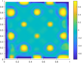
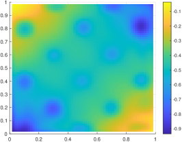
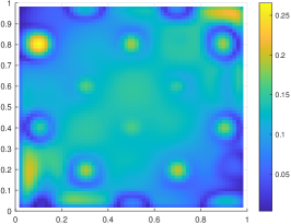
Figure 4. Left: control signal $u_{\gamma_{*}}(x)$. Middle: mean $\mathbb{E}[y(u_{\gamma_{*}},\omega,x)]$. Right: standard deviation $\sqrt{\mathbb{E}[(y(u_{\gamma_{*}},\omega,x)-\mathbb{E}[y(u_{\gamma_{*}},\omega,x)])^{2}]}$.

6.3. Variational inequality constraints

In this section we minimize the regularized misfit

$$j(u)=\frac{1}{2}\mathbb{E}[\|y(u,\omega,x)-y_{d}(x)\|_{L^{2}(D)}^{2}]+\frac{1}{2}\|u(x)\|_{L^{2}(D)}^{2}$$ (6.8)

subject to a random elliptic variational inequality (VI) constraint,

$$y(u,\omega,x)\leq 0\mathrel{\mathop{\mathchar 58\relax}}\quad\langle A(\omega)y(u,\omega,x)-f(\omega,x)-B(\omega,x)u,y(u,\omega,x)-v\rangle\leq 0,\quad\forall v\mathrel{\mathop{\mathchar 58\relax}}v\leq 0.$$ (6.9)

We use Example 5.1 from [1] (with the reversed sign of $y$), where $D=(0,1)^{2}$, $A=-\Delta$, $B=\mathrm{Id}$, and deterministic functions constructing the desired state:

$$\hat{y}(x) =\begin{cases}160(x_{1}^{3}-x_{1}^{2}+0.25x_{1})(x_{2}^{3}-x_{2}^{2}+0.25x_{2})&\mbox{in }(0,0.5)^{2},\\ 0,&\mbox{otherwise},\end{cases}$$

$$\hat{\zeta}(x) =\max(0,-2|x_{1}-0.8|-2|x_{1}x_{2}-0.3|+0.5),$$

$$y_{d}(x) =-\hat{y}-\hat{\zeta}+\Delta\hat{y}.$$

In contrast, the right hand side depends on the random variables,

$$f(\xi(\omega),x) =\Delta\hat{y}+\hat{y}+\hat{\zeta}+b(\xi(\omega),x),$$

$$b(\xi(\omega),x) =\begin{cases}\sum_{i=1}^{d}\sqrt{\lambda_{i}}\phi_{i}(x)\xi_{i}(\omega),&\mbox{in }(0,0.5)\times(0,1),\\ 0,&\mbox{otherwise}.\end{cases}$$

The Karhunen-Loeve expansion in $b(\xi,x)$ is an affine-uniform random field, with $\xi_{i}(\omega)\sim\mathcal{U}(-1,1)$, $\phi_{i}(x)=2\cos(\pi jx_{2})\cos(\pi kx_{1})$ and $\lambda_{i}=\frac{1}{100}\exp(-\frac{\pi}{4}(j^{2}+k^{2}))$, where the pairs $(j,k)$, $j,k=1,2,\ldots,$ are permuted such that $\lambda_{1}\geq\lambda_{2}\geq\cdots$.

The VI (6.9) is replaced by the penalized problem

$$Ay+\frac{1}{\varepsilon}g_{\varepsilon}(y)=f(\xi,x)+Bu,$$ (6.10)

so we minimize (6.8) with $y(u,\xi,x)$ plugged in from (6.10). The latter equation is solved via the Newton method, initialized with $y=0$ as the initial guess, and stopped when the relative difference between two consecutive iterations of $y$ falls below $10^{-12}$. The problem is discretized in $x$ via the piecewise bilinear finite elements on a uniform $n_{y}\times n_{y}$ grid with cell size $h=1/(n_{y}+1)$. The homogeneous Dirichlet boundary conditions $y=0$ on $\partial D$ allow us to store only interior grid points. This gives us a discrete problem of minimizing

$$j^{h}(\mathbf{u})=\frac{1}{2}\mathbb{E}[\|\mathbf{y}(\mathbf{u},\xi)-\mathbf{y}_{d}\|_{\mathbf{M}_{h}}^{2}]+\frac{1}{2}\|\mathbf{u}\|_{\mathbf{M}_{h}}^{2}$$ (6.11)

subject to

$$\mathbf{A}_{h}\mathbf{y}+\frac{1}{\varepsilon}g_{\varepsilon}(\mathbf{y})=\mathbf{f}(\xi)+\mathbf{u},$$ (6.12)

where $\mathbf{A}_{h},\mathbf{M}_{h}\in\mathbb{R}^{n_{y}^{2}\times n_{y}^{2}}$ are the stiffness and mass matrices, respectively.

The state part of the cost

$$j_{y}(\mathbf{u},\xi)=\frac{1}{2}\|\mathbf{y}(\mathbf{u},\xi)-\mathbf{y}_{d}\|_{\mathbf{M}_{h}}^{2}$$

and its gradient

$$\nabla_{u}j_{y}(\mathbf{u},\xi)=\mathbf{S}_{h}^{*}(\xi)\mathbf{M}_{h}(\mathbf{y}(\mathbf{u},\xi)-\mathbf{y}_{d})$$

are approximated by the TT-Cross (as functions of $\xi$), which allows one to compute the expectation of $\tilde{j}_{y}(\mathbf{u},\xi)\approx j_{y}(\mathbf{u},\xi)$ and $\nabla_{u}\tilde{j}_{y}(\mathbf{u},\xi)\approx\nabla_{u}j_{y}(\mathbf{u},\xi)$ easily. The forward model (6.12) is solved at each evaluation of $\xi$ in the TT-Cross. However, to avoid excessive computations, the Hessian of (6.11) is approximated by that anchored at the mean point $\xi=0$:

$$\nabla_{uu}j^{h}(\mathbf{u})\approx\mathbf{\tilde{H}}\mathrel{\mathop{\mathchar 58\relax}}=\mathbf{S}_{h}^{*}(0)\mathbf{M}_{h}\mathbf{S}_{h}^{\prime}(0)+\mathbf{M}_{h}.$$

The Newton system $\mathbf{\tilde{H}}^{-1}\nabla_{u}j^{h}$ is solved iteratively by using the CG method, since the matrix-vector product with $\mathbf{\tilde{H}}$ requires the solution of only one forward and one adjoint problem,

$$\mathbf{S}_{h}^{*}\cdot\mathbf{v}=\mathbf{S}_{h}^{\prime}\cdot\mathbf{v}=\left(\mathbf{A}_{h}+\mathrm{diag}\left(\frac{1}{\varepsilon}g_{\varepsilon}^{\prime}(\mathbf{y})\right)\right)^{-1}\mathbf{v},\quad\forall\mathbf{v}\in\mathbb{R}^{n_{y}^{2}}.$$ (6.13)

In Table 1 we vary the dimension of the random variable $d$, the number of quadrature points in each random variable $n_{\xi}$, and the approximation tolerance in the TT-Cross (tol). The spatial grid size is fixed to $n_{y}=31$, which is comparable with the resolution in [1], and the smoothing parameter $\varepsilon=10^{-6}$. As a reference solution $\mathbf{u}_{*}$, we take the control computed with $d=20$, $n_{\xi}=5$ and $\mbox{tol}=10^{-4}$. We see that the control and the cost can be approximated quite accurately even with a very low order of the polynomial approximation in $\xi$. It also seems unnecessary to keep $20$ terms in the Karhunen-Loeve expansion.

The computation complexity is dominated by the solutions of the forward and adjoint problems. The article [1] reports a “# PDE solves” in a path-following stochastic variance reduced gradient method solving (6.8)–(6.9). We believe this indicates the number of the complete solutions of the PDE (6.12). However, each solution of (6.12) to the increment tolerance $10^{-12}$ requires 23–25 Newton iterations, each of which requires the linear system solution of the form (6.13), Moreover, the anchored outer Hessian $\mathbf{\tilde{H}}$ requires two extra linear solves. Therefore, in Table 1, we show both the number of PDE solutions till convergence, $N_{pde}$, and the number of all linear system solutions $N_{lin}$, occurred during the optimization of (6.11) till the relative increment of $\mathbf{u}$ falls below the TT-Cross tolerance. In addition, we report the maximal TT ranks of the state cost gradient and the state itself. Note that assembly of the full state is not needed during the optimization of (6.11) – only certain samples of $\mathbf{y}(\mathbf{u},\xi)$ are needed in the TT-Cross approximation of $\nabla_{u}j^{h}$. To save the computing time, the TT tensor of the entire state is computed only after the optimization of $\mathbf{u}$ has converged.

Table 1. Cost, error in the control, number of solutions of $n_{y}^{2}\times n_{y}^{2}$ linear system as in (6.13), number of complete forward PDE solutions (6.12), and the TT ranks of the cost gradient and forward solution.

$d$	$n_{\xi}$	tol	$j^{h}(\mathbf{u})$	$\frac{\|\mathbf{u}-\mathbf{u}_{*}\|_{\mathbf{M}_{h}}}{\|\mathbf{u}_{*}\|_{\mathbf{M}_{h}}}$	$N_{lin}$	$N_{pde}$	$r(\nabla_{u}\tilde{j}_{y})$	$r(\mathbf{\tilde{y}})$
10	5	$10^{-4}$	1.261333069	1.1473e-06	1070007	44584	85	316
20	3	$10^{-3}$	1.261333069	2.9012e-05	46312	1976	7	29
20	3	$10^{-4}$	1.261333069	4.2713e-06	433134	18153	56	183
20	5	$10^{-4}$	1.261333069	—	1840467	76243	102	402

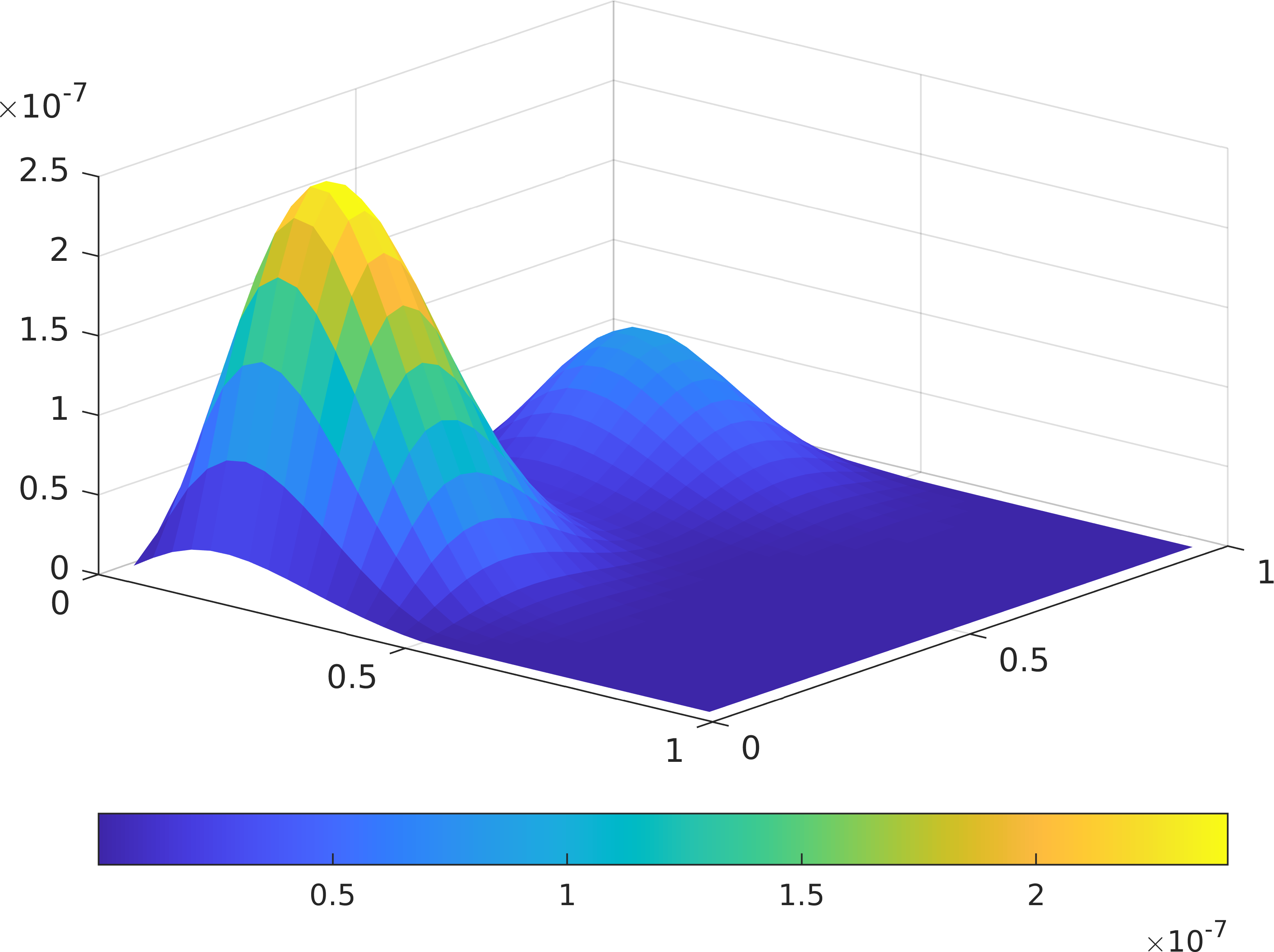
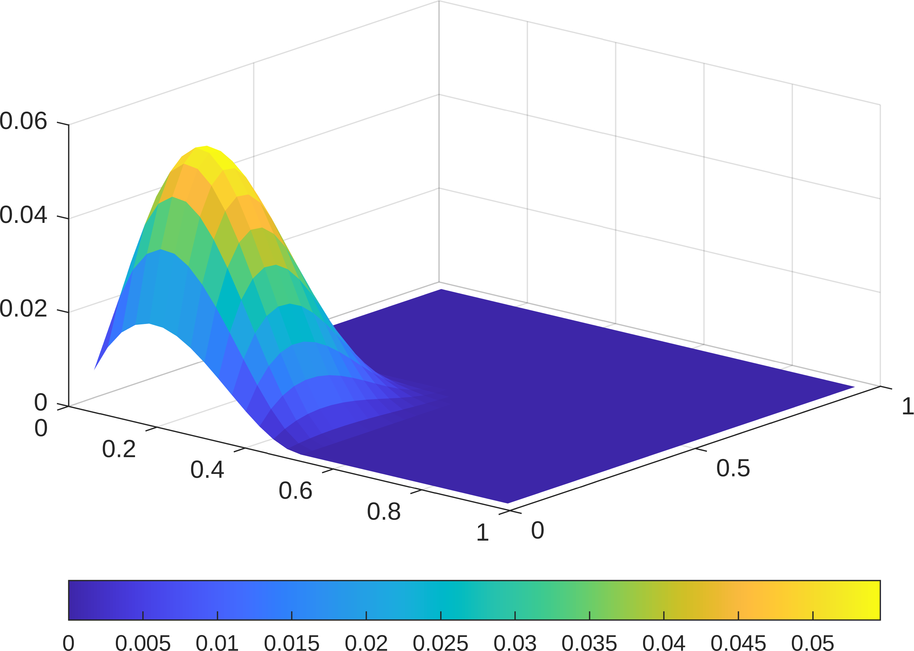
Figure 5. Left: mean optimised state $\mathbb{E}[-y]$ with $d=20,$ $n_{\xi}=3$ and $\mbox{tol}=10^{-3}$. Middle: variance of the optimized state $\mathbb{E}[(y-\mathbb{E}[y])^{2}]$. Right: optimised control $u$.

In Figure 5 we show the mean optimized forward state and the control. The results coincide qualitatively with those in [1]. If we consider the computational cost necessary to compute the optimal control only, we can notice that $N_{pde}$ is significantly lower than the 291808 PDE solves in the stochastic variance reduced gradient method of [1].

6.4. SEIR ODE model

Now consider a slightly simplified version of the epidemiological ODE model used for the propagation of COVID-19 in the UK using the data from March-May 2020 [11]. This is a compartmental differential equation model with the following compartments.

• Susceptible ($S$).

• Exposed ($E$), but not yet infectious.

• Infected SubClinical type 1 ($I^{SC1}$): may require hospitalization in the future.

• Infected SubClinical type 2 ($I^{SC2}$): will recover without hospitalization.

• Infected Clinical type 1 ($I^{C1}$): individuals in the hospital who may decease.

• Infected Clinical type 2 ($I^{C2}$): individuals in the hospital who will recover.

• Recovered ($R$) and immune to reinfections.

• Deceased ($D$).

In turn, each of these compartments are split into 5 further sub-compartments corresponding to age bands: 0-19, 20-39, 40-59, 60-79 and 80+. The number of individuals in each compartment is denoted by the name of the compartment and age band index, For example, $S_{i}$ denotes the number of susceptible individuals in the $i$th age band ($i=1,\ldots,5$), $E_{i}$ denotes the number of exposed individuals in the $i$th age band, and so on. Variables corresponding to different age bands but same compartment are collected into vectors, $S=(S_{1},\ldots,S_{5})$, $E=(E_{1},\ldots,E_{5})$ and so on.

Some of the variables introduced above are coupled to others only one way, and can be removed from the actual simulations. First, when the number of infected individuals is small compared to the population size (which is typically the case in the early stages of the epidemic), the relative variation of $S$ is small. Hence, $S$ can be taken constant instead of solving an ODE on it. Similarly, none of the variables depend on $R$ and $D$, so they can be excluded from a coupled system of ODEs too, and computed separately after the solution of the ODEs. With these considerations in mind, the forward model reads as follows:

$$\frac{d}{dt}\begin{bmatrix}E\\ I^{SC1}\\ I^{SC2}\\ I^{C1}\\ I^{C2}\end{bmatrix} -\begin{bmatrix}-\kappa\mathtt{I}&A_{u}&A_{u}&0&0\\ \kappa\cdot\mathrm{diag}(\rho)&-\eta_{C}\mathtt{I}&0&0&0\\ \kappa\cdot\mathrm{diag}(1-\rho)&0&-\eta_{R}\mathtt{I}&0&0\\ 0&\eta_{C}\cdot\mathrm{diag}(\rho^{\prime})&0&-\nu\mathtt{I}&0\\ 0&\eta_{C}\cdot\mathrm{diag}(1-\rho^{\prime})&0&0&-\eta_{R,C}\mathtt{I}\end{bmatrix}\begin{bmatrix}E\\ I^{SC1}\\ I^{SC2}\\ I^{C1}\\ I^{C2}\end{bmatrix}=0.$$ (6.14)

Here $\mathtt{I}\in\mathbb{R}^{5\times 5}$ is the identity matrix and $\mathrm{diag}(\cdot)$ produces a diagonal matrix from a vector. The control is defined in terms of the intensity of lockdown measures, and affects the susceptible-infected interaction matrix $A_{u}=\chi\cdot\mathrm{diag}(S)\cdot C_{u}\cdot\mathrm{diag}(\frac{1}{N})$, where

$$C_{u}=\mathrm{diag}(c^{home})C^{home}+\mathrm{diag}(c^{work}_{u})C^{work}+\mathrm{diag}(c^{school}_{u})C^{school}+\mathrm{diag}(c^{other}_{u})C^{other}$$ (6.15)

is the matrix of contact intensities between the age compartments. The total contact intensity is a sum of pre-pandemic contact intensity matrices in the four setting $C^{home},C^{work},C^{school}$ and $C^{other}$, multiplied by the reduction factors $c^{home},c^{work}_{u},c^{school}_{u}$ and $c^{other}_{u}$ due to the lockdown measures. Since home contacts cannot be controlled, $c^{home}=(1,\ldots,1)$, but the remaining factors vary proportionally to the lockdown control applied from day 17 onwards,

$$c^{\mu}_{u}(t)=\left\{\begin{array}[]{ll}(1,1,1,1,1)^{\top},&t<17,\\ (c_{123}(1-u^{\mu}(t)),c_{123}(1-u^{\mu}(t)),c_{123}(1-u^{\mu}(t)),c_{4},c_{5})^{\top},&17\leq t\leq 90,\\ (c_{123}(1-u^{\mu}(90)),c_{123}(1-u^{\mu}(90)),c_{123}(1-u^{\mu}(90)),c_{4},c_{5})^{\top},&t>90,\end{array}\right.$$ (6.16)

where $\mu\in\{work,school,other\}$, $u^{\mu}$ are the intensities of lockdown measures applied to each setting $\mu$, and $c_{123},c_{4},c_{5}$ are the initial contact intensities in the corresponding age groups. Note that the control will be optimized only on the time interval $[17,90]$. Before day 17 the contact intensities are not reduced (no lockdown). From day 90 onwards we continue applying the last value of the control.

In addition, the model depends on the following parameters:

• $\chi$: probability of $S$–$I^{SC}$ interactions.

• $\kappa=1/d_{L}$: average rate of an Exposed individual becoming SubClinical. It is inversely proportional to the average number of days $d_{L}$ an individual stays in the Exposed state.

• $\eta_{C}=1/d_{C}$: average rate of a SubClinical individual becoming Clinical. Similarly, $d_{C}$ is the average time spent in the SubClinical state.

• $\eta_{R}=1/d_{R}$: rate of recovery from $I^{SC2}$.

• $\eta_{R,C}=1/d_{R,C}$: rate of recovery from $I^{C2}$.

• $\nu=1/d_{D}$: rate of decease in the $I^{C1}$ state.

• $\rho=(\rho_{1},\ldots,\rho_{5})^{\top}\in\mathbb{R}^{5}$: correction coefficients of the Exposed $\rightarrow$ SubClinical 1 transition rate for different age bands.

• $\rho^{\prime}=(\rho^{\prime}_{1},\ldots,\rho^{\prime}_{5})^{\top}\in\mathbb{R}^{5}$: correction coefficients of the SubClinical $\rightarrow$ Clinical 1 transition.

• $N=(N_{1},\ldots,N_{5})^{\top}\in\mathbb{R}^{5}$: total number of individuals in each age group.

• $N^{0}$: total number of infected individuals on day 0.

• $N^{in}=(0.1,0.4,0.35,0.1,0.05)^{\top}N^{0}$: age partition of the initial number of infected individuals.

The ODE (6.14) is initialized by setting

$$E(0)=\frac{N^{in}}{3},\quad I^{SC1}(0)=\frac{2}{3}\mathrm{diag}(\rho)N^{in},\quad I^{SC2}(0)=\frac{2}{3}\mathrm{diag}(1-\rho)N^{in},\quad I^{C1}(0)=I^{C2}(0)=0.$$

The population sizes $S=N$ are taken from the Office for National Statistics, mid 2018 estimate.

However, none of the model parameters above are known beforehand. In [11], those were treated as random variables, and their distributions were estimated from observed numbers of infections and hospitalizations during the first $90$ days using Approximate Bayesian Computation (ABC). In general, these variables are correlated through the posterior distribution, sampling from which is a daunting problem. Here, we replace the joint ABC posterior distribution by independent uniform distributions with a scaled posterior standard deviation centered around the posterior mean:

$$\chi \sim\mathcal{U}(0.13-0.03\sigma,0.13+0.03\sigma), d_{L} \sim\mathcal{U}(1.57-0.42\sigma,1.57+0.42\sigma),$$ (6.17)

$$d_{C} \sim\mathcal{U}(2.12-0.80\sigma,2.12+0.80\sigma), d_{R} \sim\mathcal{U}(1.54-0.40\sigma,1.54+0.40\sigma),$$

$$d_{R,C} \sim\mathcal{U}(12.08-1.51\sigma,12.08+1.51\sigma), d_{D} \sim\mathcal{U}(5.54-2.19\sigma,5.54+2.19\sigma),$$

$$\rho_{1} \sim\mathcal{U}(0.06-0.03\sigma,0.06+0.03\sigma), \rho_{2} \sim\mathcal{U}(0.05-0.03\sigma,0.05+0.03\sigma),$$

$$\rho_{3} \sim\mathcal{U}(0.08-0.04\sigma,0.08+0.04\sigma), \rho_{4} \sim\mathcal{U}(0.54-0.22\sigma,0.54+0.22\sigma),$$

$$\rho_{5} \sim\mathcal{U}(0.79-0.14\sigma,0.79+0.14\sigma), \rho^{\prime}_{1} \sim\mathcal{U}(0.26-0.23\sigma,0.26+0.23\sigma),$$

$$\rho^{\prime}_{2} \sim\mathcal{U}(0.28-0.25\sigma,0.28+0.25\sigma), \rho^{\prime}_{3} \sim\mathcal{U}(0.33-0.27\sigma,0.33+0.27\sigma),$$

$$\rho^{\prime}_{4} \sim\mathcal{U}(0.26-0.11\sigma,0.26+0.11\sigma), \rho^{\prime}_{5} \sim\mathcal{U}(0.80-0.13\sigma,0.80+0.13\sigma),$$

$$N^{0} \sim\mathcal{U}(276-133\sigma,276+133\sigma), c_{123} \sim\mathcal{U}(0.63-0.21\sigma,0.63+0.21\sigma),$$

$$c_{4} \sim\mathcal{U}(0.57-0.23\sigma,0.57+0.23\sigma), c_{5} \sim\mathcal{U}(0.71-0.23\sigma,0.71+0.23\sigma).$$

Here, $\sigma$ is the standard deviation scaling parameter, taken to be $0.03$ in our experiment. This distribution behaves qualitatively similar to the posterior distribution in the vicinity of the posterior mean. It provides sufficient randomness to benchmark the constrained optimization method, while admitting independent sampling and gridding, needed for the TT approximations. That is, (6.17) form a random vector

$$\xi=(\chi,d_{L},d_{C},d_{R},d_{R,C},d_{D},\rho_{1},\rho_{2},\rho_{3},\rho_{4},\rho_{5},\rho^{\prime}_{1},\rho^{\prime}_{2},\rho^{\prime}_{3},\rho^{\prime}_{4},\rho^{\prime}_{5},N^{0},c_{123},c_{4},c_{5})$$

of $d=20$ independent random variables, the state vector is

$$y(\xi,t)=(E_{1},\ldots,E_{5},~{}I^{SC1}_{1},\ldots,I^{SC1}_{5},~{}I^{SC2}_{1},\ldots,I^{SC2}_{5},~{}I^{C1}_{1},\ldots,I^{C1}_{5},~{}I^{C2}_{1},\ldots,I^{C2}_{5}),$$

and the ODE (6.14) constitutes the forward problem.

For the inverse problem, we use the total number of deceased patients as the cost function. The rate of decease is proportional to the number of Clinical type 1 individuals, so the total number of deceased individuals can be computed as

$$D(\xi,t)=\nu\int_{0}^{t}I^{C1}(\xi,s)ds.$$ (6.18)

To regularize the problem, we add also the norm of the control $u(t)=(u^{work}(t),u^{school}(t),u^{other}(t))$. Thus, the total cost function reads

$$j(u)=\frac{1}{2}\mathbb{E}[D(\xi,T)]+\frac{\alpha}{2}\int_{17}^{90}\|u(t)\|_{2}^{2}dt,$$ (6.19)

where $T=100$ is the final simulation time, and $\alpha$ is the regularization parameter, which we set to $100$ in our experiment. Note that the norm of the control is taken only over the time interval $[17,90]$ where the control varies.

We introduce the following constraints. Firstly, we limit the control components to the intervals $u^{work}\in[0,0.69]$, $u^{school}\in[0,0.9]$ and $u^{other}\in[0,0.59]$. Next, we constrain the $\mathcal{R}$ number at the end of the variable control interval, $\mathcal{R}(\xi,90)\leq 1$. In our model, the $\mathcal{R}$ number can be computed as $\mathcal{R}(\xi,t)=\lambda_{\max}(K),$ where

$$K=-\begin{bmatrix}0&A_{u}&A_{u}&0&0\\ 0&0&0&0&0\\ 0&0&0&0&0\\ 0&0&0&0&0\\ 0&0&0&0&0\\ \end{bmatrix}\begin{bmatrix}-\kappa\mathtt{I}&0&0&0&0\\ \kappa\cdot\mathrm{diag}(\rho)&-\eta_{C}\mathtt{I}&0&0&0\\ \kappa\cdot\mathrm{diag}(1-\rho)&0&-\eta_{R}\mathtt{I}&0&0\\ 0&\eta_{C}\cdot\mathrm{diag}(\rho^{\prime})&0&-\nu\mathtt{I}&0\\ 0&\eta_{C}\cdot\mathrm{diag}(1-\rho^{\prime})&0&0&-\eta_{R,C}\mathtt{I}\end{bmatrix}^{-1},$$

and $\lambda_{\max}$ denotes the maximal in modulus eigenvalue. Recall that $\mathcal{R}<1$ implies that the epidemic decays, while $\mathcal{R}>1$ corresponds to an expanding epidemic. The full smoothed Moreau-Yosida cost function becomes

$$j^{\gamma,\varepsilon}(u)=\frac{1}{2}\mathbb{E}[D(\xi,T)]+\frac{\alpha}{2}\int_{17}^{90}\|u(t)\|_{2}^{2}dt+\frac{\gamma}{2}\mathbb{E}\left[\left|g_{\varepsilon}(\mathcal{R}(\xi,90)-1)\right|^{2}\right].$$ (6.20)

Since the control is applied nonlinearly in the model, computation of derivatives of the cost function (6.20) is complicated. Thus, instead of the Newton method, we use the projected gradient descent method, where the gradient of (6.20) is calculated using finite differencing with anisotropic step sizes $10^{-6}\cdot\max(|u|,0.1)$. The ODE (6.14) is solved using an implicit Euler method with a time step $0.1$. In this experiment, we use a fixed Moreau-Yosida parameter $\gamma=5\cdot 10^{5}$ in all iterations, and the smoothing width is chosen as $\varepsilon=50/\sqrt{\gamma}$. The iteration is stopped when the cost value does not decrease in two consecutive iterations. Each random variable (6.17) is discretized with $n=3$ Gauss-Legendre quadrature nodes, and the TT approximations are carried out with a relative error tolerance of $10^{-2}$. The control $u(t)$ is discretized using $7$ Gauss-Legendre nodes on $[17,90]$ with a Lagrangian interpolation in between.

Figure 6. Top: optimized $I^{C}=I^{C1}+I^{C2}$, mean (blue circles) and 95% confidence interval (shaded area). Bottom: optimized control signals. Left: unconstrained optimization, Right: optimization constrained with $\mathcal{R}(\xi,90)\leq 1$ a.s. approximated with $\gamma=5\cdot 10^{5}$. Black dashed lines indicate the end of the optimization time horizon $t=90$.

In Figure 6, we compare optimizations without constraining $\mathcal{R}(\xi,90)$ (left), and with the a.s. constraint (right) as described above. We plot the time evolution of the mean and confidence interval of the total number of hospitalized individuals, $I^{C}(t)=I^{C1}(t)+I^{C2}(t)$. The unconstrained scenario is a finite horizon optimization problem, which drives the control to near zero values at the end of the controllable time interval, $t=90$, due to the zero terminal condition on the adjoint state. Naturally, this leads to infection growing again for $t>90$, since we extrapolate these small values of the control from $t=90$ onwards.

In contrast, if we constrain the $\mathcal{R}$ number at the end of the optimization interval to be below $1$ almost surely, this drives the control to higher values again. If we extrapolate these control values beyond the optimization window, the epidemic continues decaying, albeit with a slightly larger uncertainty. This indicates that almost sure constraints can suggest a more resilient control in risk-critical applications.

Appendix A Proof of Lemma 3.11

Introduce a new variable $t=\exp(s/\varepsilon)$, then

$$\int_{-\infty}^{0}s\log(1+\exp(s/\varepsilon))ds =\int_{0}^{1}\frac{\varepsilon\log(t)\log(1+t)}{t/\varepsilon}dt$$

$$=\varepsilon^{2}\int_{0}^{1}\log(t)\log(t+1)d\log(t)$$

$$=\frac{\varepsilon^{2}}{2}\left.(\log(t))^{2}\log(t+1)\right|_{0}^{1}-\frac{\varepsilon^{2}}{2}\int_{0}^{1}(\log(t))^{2}d\log(t+1).$$

The first term is zero at $t=1$, and at $t=0$ we can use that $0\leq\log(t+1)\leq t$ for $0\leq t<1$ and $\lim_{t\rightarrow 0}(\log(t))^{2}\log(t+1)\leq\lim_{t\rightarrow 0}(\log(t))^{2}t=0.$ For the second term, we proceed as follows,

$$\int_{-\infty}^{0}s\log(1+\exp(s/\varepsilon))ds =-\frac{\varepsilon^{2}}{2}\int_{0}^{1}\frac{(\log(t))^{2}}{t+1}dt$$

$$\geq-\frac{\varepsilon^{2}}{2}\int_{0}^{1}(\log(t))^{2}dt$$

$$=-\frac{\varepsilon^{2}}{2}\underbrace{\left.t(\log(t))^{2}\right|_{0}^{1}}_{0}+\varepsilon^{2}\int_{0}^{1}\log(t)dt$$

$$=\varepsilon^{2}\left.t\log t\right|_{0}^{1}-\varepsilon^{2}\int_{0}^{1}dt=-\varepsilon^{2}.$$

The proof is completed by recalling that $sg_{\varepsilon}(s)=\varepsilon\cdot s\log(1+\exp(s/\varepsilon))$.

References

- [1] A. Alphonse, C. Geiersbach, M. Hintermüller, and T. M. Surowiec. Risk-averse optimal control of random elliptic variational inequalities. arXiv preprint 2210.03425, 2022.
- [2] H. Antil, T.S. Brown, D. Verma, and M. Warma. Optimal control of fractional PDEs with state and control constraints. Pure Appl. Funct. Anal., 7(5):1533–1560, 2022.
- [3] H. Antil, S. Dolgov, and A. Onwunta. Ttrisk: Tensor train decomposition algorithm for risk averse optimization. Numerical Linear Algebra with Applications, n/a(n/a):e2481.
- [4] H. Antil, D.P. Kouri, M.-D. Lacasse, and D. Ridzal, editors. Frontiers in PDE-constrained optimization, volume 163 of The IMA Volumes in Mathematics and its Applications. Springer, New York, 2018. Papers based on the workshop held at the Institute for Mathematics and its Applications, Minneapolis, MN, June 6–10, 2016.
- [5] D. Bigoni, A. P. Engsig-Karup, and Y. M. Marzouk. Spectral tensor-train decomposition. SIAM J. Sci. Comput., 38(4):A2405–A2439, 2016.
- [6] E. Casas. Control of an elliptic problem with pointwise state constraints. SIAM J. Control Optim., 24(6):1309–1318, 1986.
- [7] S. Dolgov, B. N. Khoromskij, A. Litvinenko, and H. G. Matthies. Polynomial Chaos Expansion of random coefficients and the solution of stochastic partial differential equations in the Tensor Train format. SIAM J. Uncertainty Quantification, 3(1):1109–1135, 2015.
- [8] S. Dolgov and D. Savostyanov. Parallel cross interpolation for high–precision calculation of high–dimensional integrals. Comput. Phys. Commun., 246:106869, 2020.
- [9] S. V. Dolgov, B. N. Khoromskij, I. V. Oseledets, and D. V. Savostyanov. Computation of extreme eigenvalues in higher dimensions using block tensor train format. Comput. Phys. Commun., 185(4):1207–1216, 2014.
- [10] S. V. Dolgov and D. V. Savostyanov. Alternating minimal energy methods for linear systems in higher dimensions. SIAM Journal on Scientific Computing, 36(5):A2248–A2271, 2014.
- [11] R. Dutta, S. N. Gomes, D. Kalise, and L. Pacchiardi. Using mobility data in the design of optimal lockdown strategies for the COVID-19 pandemic. PLoS Comput. Biol., 17(8):1–25, 2021.
- [12] M. H. Farshbaf-Shaker, R. Henrion, and D. Hömberg. Properties of chance constraints in infinite dimensions with an application to PDE constrained optimization. Set-Valued Var. Anal., 26(4):821–841, 2018.
- [13] D.B. Gahururu, M. Hintermüller, and T.M. Surowiec. Risk-neutral pde-constrained generalized nash equilibrium problems. Mathematical Programming, 2022.
- [14] S. Garreis, T. M. Surowiec, and M. Ulbrich. An interior-point approach for solving risk-averse PDE-constrained optimization problems with coherent risk measures. SIAM J. Optim., 31(1):1–29, 2021.
- [15] C. Geiersbach and W. Wollner. Optimality conditions for convex stochastic optimization problems in Banach spaces with almost sure state constraints. SIAM J. Optim., 31(4):2455–2480, 2021.
- [16] Caroline Geiersbach and Michael Hintermüller. Optimality Conditions and Moreau–Yosida Regularization for Almost Sure State Constraints. ESAIM Control Optim. Calc. Var., 28:Paper No. 80, 36, 2022.
- [17] A. Geletu, A. Hoffmann, P. Schmidt, and P. Li. Chance constrained optimization of elliptic PDE systems with a smoothing convex approximation. ESAIM Control Optim. Calc. Var., 26:Paper No. 70, 28, 2020.
- [18] S. A. Goreinov, I. V. Oseledets, D. V. Savostyanov, E. E. Tyrtyshnikov, and N. L. Zamarashkin. How to find a good submatrix. In V. Olshevsky and E. Tyrtyshnikov, editors, Matrix Methods: Theory, Algorithms, Applications, pages 247–256. World Scientific, Hackensack, NY, 2010.
- [19] A. Gorodetsky, S. Karaman, and Y. Marzouk. A continuous analogue of the tensor-train decomposition. Comput. Methods Appl. Mech. Engrg., 347:59–84, 2019.
- [20] W. Hackbusch and B. N. Khoromskij. Low-rank Kronecker-product approximation to multi-dimensional nonlocal operators. I. Separable approximation of multi-variate functions. Computing, 76(3-4):177–202, 2006.
- [21] M. Hintermüller and M. Hinze. Moreau-Yosida regularization in state constrained elliptic control problems: Error estimates and parameter adjustment. SIAM Journal on Numerical Analysis, 47(3):1666–1683, 2009.
- [22] M. Hoffhues, W. Römisch, and T. M. Surowiec. On quantitative stability in infinite-dimensional optimization under uncertainty. Optimization Letters, 15(8):2733–2756, 2021.
- [23] D. P. Kouri and T. M. Surowiec. Risk-averse PDE-constrained optimization using the conditional value-at-risk. SIAM J. Optim., 26(1):365–396, 2016.
- [24] K. Kunisch and D. Wachsmuth. Sufficient optimality conditions and semi-smooth Newton methods for optimal control of stationary variational inequalities. ESAIM Control Optim. Calc. Var., 18(2):520–547, 2012.
- [25] R. Löhner, H. Antil, S. Idelsohn, and E. Oñate. Detailed simulation of viral propagation in the built environment. Comput. Mech., 66(5):1093–1107, 2020.
- [26] R. Löhner, H. Antil, A. Srinivasan, S Idelsohn, and E. Oñate. High-fidelity simulation of pathogen propagation, transmission and mitigation in the built environment. Archives of Computational Methods in Engineering, pages 1–26, 2021.
- [27] G. J. Lord, C. E. Powell, and T. Shardlow. An Introduction to Computational Stochastic PDEs. West Nyack: Cambridge University Press, 2014.
- [28] K. Maute. Topology optimization under uncertainty. In Topology optimization in structural and continuum mechanics, pages 457–471. Springer, 2014.
- [29] A. Yu. Mikhalev and I. V. Oseledets. Rectangular maximum–volume submatrices and their applications. Linear Algebra Appl., 538:187–211, 2018.
- [30] I. V. Oseledets. Tensor train decomposition. SIAM J. Sci. Comp., 33(5):2295 – 2317, 2011.
- [31] I. V. Oseledets and E. E. Tyrtyshnikov. TT-cross approximation for multidimensional arrays. Linear Algebra Appl., 432(1):70–88, 2010.
- [32] R. T. Rockafellar and S. Uryasev. Optimization of conditional value-at-risk. The Journal of Risk, 2:21 – 41, 2000.
- [33] P. B. Rohrbach, S. Dolgov, L. Grasedyck, and R. Scheichl. Rank bounds for approximating Gaussian densities in the Tensor-Train format. SIAM/ASA Journal on Uncertainty Quantification, 10(3):1191–1224, 2022.
- [34] D. V. Savostyanov and I. V. Oseledets. Fast adaptive interpolation of multi-dimensional arrays in tensor train format. In Proceedings of 7th International Workshop on Multidimensional Systems (nDS). IEEE, 2011.
- [35] R. Schneider and A. Uschmajew. Approximation rates for the hierarchical tensor format in periodic Sobolev spaces. J. Complexity, 2013.
- [36] J. Sokołowski and J. P. Zolésio. Introduction to shape optimization, volume 16 of Springer Series in Computational Mathematics. Springer-Verlag, Berlin, 1992. Shape sensitivity analysis.
- [37] L. N. Trefethen. Spectral methods in MATLAB. SIAM, Philadelphia, 2000.
- [38] F. Tröltzsch. Optimal Control of Partial Differential Equations: Theory, Methods and Applications. American Mathematical Society, 2010.