STORM-GAN: Spatio-Temporal Meta-GAN for Cross-City Estimation of Human Mobility Responses to COVID-19

Abstract

Human mobility estimation is crucial during the COVID-19 pandemic due to its significant guidance for policymakers to make non-pharmaceutical interventions. While deep learning approaches outperform conventional estimation techniques on tasks with abundant training data, the continuously evolving pandemic poses a significant challenge to solving this problem due to data nonstationarity, limited observations, and complex social contexts. Prior works on mobility estimation either focus on a single city or lack the ability to model the spatio-temporal dependencies across cities and time periods. To address these issues, we make the first attempt to tackle the cross-city human mobility estimation problem through a deep meta-generative framework. We propose a Spatio-Temporal Meta-Generative Adversarial Network (STORM-GAN) model that estimates dynamic human mobility responses under a set of social and policy conditions related to COVID-19. Facilitated by a novel spatio-temporal task-based graph (STTG) embedding, STORM-GAN is capable of learning shared knowledge from a spatio-temporal distribution of estimation tasks and quickly adapting to new cities and time periods with limited training samples. The STTG embedding component is designed to capture the similarities among cities to mitigate cross-task heterogeneity. Experimental results on real-world data show that the proposed approach can greatly improve estimation performance and outperform baselines.

I Introduction

Evolving developments (e.g., spread, mutation, vaccination) around the COVID-19 pandemic have continued to pressure policymakers to come up with effective and changing policies that can protect public health while avoiding breakdowns of economics, and maintain the support of essential needs in daily lives. To mitigate this dilemma, staged reopening to avoid infections caused by eased social distancing policies have been implemented. As a result, estimation on dynamic human mobility responses to the pandemic condition and policies remains a crucial task in policymaking.

Due to the asynchronous spread of the disease, it is particularly hard for cities in the early stage of an outbreak or wave (e.g., the Omicron variant) to estimate future human mobility responses under unprecedented severity levels or unseen policies as there is very limited historical data. To address this issue, it is crucial for such cities to be able to leverage other cities’ past experiences and knowledge for its own estimation. To this end, mobility response estimation methods that can leverage cross-city knowledge to achieve promising results are urgently needed.

In this paper, we make the first attempt to solve the cross-city human mobility responses estimation problem: Given a set of inputs on contextual (e.g., population, point-of-interest POI counts), epidemic (e.g., COVID-19 cases), policy (e.g., stay-at-home orders) conditions and corresponding human mobility responses measures (e.g., POI visit counts, home dwell time) from multiple cities, we aim to learn a model, which can quickly adapt to previously unseen cities and time periods, and estimate human mobility response dynamics under any projected conditions.

Challenges. The cross-city human mobility response estimation problem has three major challenges. First, human mobility responses depend on many complex social-physical factors which are unknown or uncertain. For example, responses can be affected by people’s willingness in cooperating with policies, decisions from service providers (e.g, whether a restaurant will open or allow dine-in options), changes in public transportation, supply, and many more [1]. Second, human mobility responses often have spatio-temporal non-stationarity. For example, the contribution of different factors in mobility tends to vary from region to region due to cultural and economic differences, and can quickly evolve over time. Such spatial and temporal nonstationarity greatly limits the availability of training data for each estimation task, making it difficult to leverage the approximation power of data-driven approaches. Third, there also exist complex spatial and temporal dependencies across different estimation tasks, i.e., cities and time periods, which need to be explicitly considered for robust parameter sharing. For example, cities may share similar mobility dynamic patterns based on their spatial adjacency (e.g., distances, travel connections such as airlines), and their stages in the pandemic.

Related Work. Many recent efforts have attempted to use machine learning methods for spatio-temporal estimation tasks. For example, [2] uses a conditional generative adversarial network (cGAN) to estimate traffic volume. Similarly, a recent work [3] proposed a COVID-GAN for human mobility estimation, where policies (e.g., school closure) are used as constraints to help improve estimation results. However, both of them only consider estimation in a single city, without modeling the spatial and temporal dependencies across cities or stages. Therefore, they lack the ability to quickly adapt to unseen cities. In addition, COVID-GAN is a purely spatial model, which does not explicitly model the dynamics of human mobility responses over time. A POI embedding transfer learning approach is proposed [4] to predict urban traffic from one city to another city. This approach adapts model parameters without using meta-learning method. In recent years, many meta-learning approaches have been proposed to solve the few-shot learning problem [5, 6], where the training samples are limited for new tasks. However, few of them are designed for spatio-temporal tasks. Among the exceptions, [7] uses a model-based meta-learning approach with a variational autoencoder structure to generate traffic volume. Another traffic prediction work [6] combines the attention mechanism and CNNs, and uses functionality zones to group cities into tasks before applying the model-agnostic meta-learning (MAML [8]) framework. However, this model is designed with no time-based tasks, which is insufficient to model the continued and dynamic changes in our problem. Moreover, it does not model and utilize the spatio-temporal dependencies and correlations across different tasks.

Proposed Work. To address the limitations of prior works, we formulate the problem as a meta-learning-based conditional data generation problem, where each task of the meta-learning framework is to estimate a time-series of human mobility response maps for a specific city during a specific time period under designated conditions. As a solution, we design a Spatio-TempORal (conditional) Meta-Generative Adversarial Network (STORM-GAN). Building on top of a conditional GAN (cGAN) model [9], the STORM-GAN model learns to generate spatio-temporal mobility dynamics in different cities under a set of geographic, epidemic, social and other factors. It utilizes a meta-learning paradigm to learn a general model initialization from a distribution of tasks (i.e., mobility estimation for each city over a time period) for fast adaption to new spatio-tempral tasks (e.g., new cities, future projection). To explicitly model the spatio-temporal relationships across tasks, we propose a Spatio-Temporal Task-based Graph (STTG) embedding method for better model generalization and adaptation, which further improves STORM-GAN’s performance. Overall, the contributions of this paper are as follows:

• We formulate the cross-city human mobility response estimation problem as a spatio-temporal meta-learning-based data generation problem. To the best of our knowledge, this is the first attempt to estimate human mobility through a deep meta-generative framework. The proposed novel meta-generative framework models the uncertainty, spatial and temporal patterns simultaneously.

• Specifically, we propose a COVID-19 spatio-temporal task-based graph, which is embedded into the framework to explicitly model spatio-temporal dependency among different tasks, further improving the learning of the shared-knowledge.

• We perform various experiments on real-world datasets to evaluate the performance of the proposed approach under different scenarios, and the results show that STORM-GAN can greatly improve mobility response estimation compared to other candidate approaches. We have released our code and the sample data in a temporary GitHub link.

II Problem Statement

This section introduces a set of basic concepts about our data modeling, and then provides a formal problem statement. The overall solution framework is shown in Fig. 1.

II-A Basic Concepts

Definition 1.

Spatial grid S is a grid-discretization of a spatial field (e.g., a city), where each grid cell $\textbf{s}_{i}$ represents an equally-sized squared area. Given S, the location of any POI can be mapped into a grid cell. For simplicity, in this work we choose the grid cells to be $1km\times 1km$.

Definition 2.

Temporal period T is a temporal period (e.g., a 7-day window) containing equal-length slots (e.g., a day), denoted as $T=\left\{t_{1},t_{2},...,t_{n}\right\}$, where each slot $t$ represents the finest temporal resolution of the data.

Definition 3.

Mobility related conditions: All conditions that will influence human mobility responses are mobility related conditions including contextual conditions (e.g., population, household income), epidemic conditions (e.g., COVID-19 confirmed cases and deaths), and policy conditions (e.g., strict stay-at-home or shelter-in-place orders). We denote a list of k conditions as $\textbf{F}=\left\{f_{1},f_{2},...,f_{k}\right\}$. For a grid cell ${s}$, we denote $f^{s,t}$ as all the conditions of ${s}$ in time slot ${t}$.

Definition 4.

Human mobility responses: The human mobility responses M is a two-dimensional tensor, representing the total number of visits to POIs (e.g., grocery stores, hardware stores, restaurants, gas stations) in each grid cell ${s}$ for time slot ${t}$.

Note here we use POI visit counts simply as an example to demonstrate the solution framework. Other mobility measures (e.g., median home dwell time) can also be used with our model. The choice of the measure is not the focus of this paper.

Definition 5.

Generator G: A deep neural network model that is used to generate a series of human mobility response maps $\textbf{M}^{\prime}_{G}$ given a set of conditions.

Definition 6.

Discriminator D: A deep neural network model that outputs a probability $p_{real}$ at which a map of human mobility responses is classified as from real-world rather than from a generator ${G}$.

Definition 7.

Spatio-temporal mobility estimation tasks: A task $\mathit{\mathcal{T}_{i}}$ consists of a series of pairs $\left(\mathbf{M}^{t},\mathbf{F}^{t}\right)$ for a few consecutive time periods ${T}$ (e.g., 5 weeks) in a partitioned area S (e.g., $10\times 10$ grids of a city). Each sample is a 4D tensor with size $l\times l\times k\times|T|$, where $l\times l$ is the size of the spatial window, and ${k}$ is the number of conditions. Each $\mathit{\mathcal{T}_{i}}$ is divided into a training set $\mathit{\mathcal{D}_{i}^{train}}$ and a testing set $\mathit{\mathcal{D}_{i}^{test}}$.

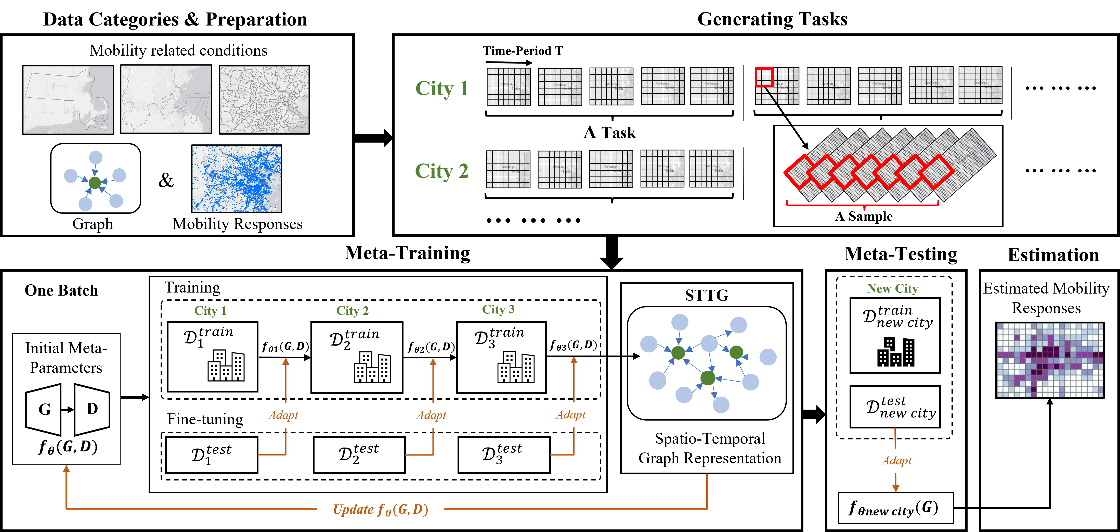
Figure 1: Overall framework.

II-B Problem Definition

We construct the tasks (Def. 7) by a spatio-temporal partition of all conditions F and mobility responses M. Each spatio-temporal task $\mathcal{T}_{i}$ contains data from the grid $S$ of a single city for $w$ consecutive time periods $\{T_{1},...,T_{w}\}$, and tasks are mutually exclusively (i.e., no overlap along the temporal dimension). Each data sample in a task contains a time-series of length $|T|$ with any start time (but the time-span of a sample must be completely within the span of a task).

Inputs:

• A time-series of conditions $\{\textbf{F}^{t-|T|+1},...,\textbf{F}^{t}\}$ for each data sample in training tasks;

• Mobility response $\textbf{M}^{t}$ for each sample in training tasks;

Outputs:

• A generator G to generate/estimate mobility responses;

• A meta-initialization $\theta$ for G for fast adaptation to training and new testing tasks.

Objective:

• Minimize average generation error on new testing tasks.

In this work, given a series of tasks sampled from multiple cities (e.g., Boston and NYC), we train a meta-generative model. When a new city (e.g., Houston) comes in with a small training set, we quickly fine-tune the meta-model parameters to obtain a tailored model for the new city to generate its mobility responses.

III Methodology

In this section, we present the details of STORM-GAN. We first present the architecture of the proposed spatio-temporal meta-generative model. Then, we show the details of meta-parameter updates in STROM-GAN. The model architecture is shown in Fig. 2.

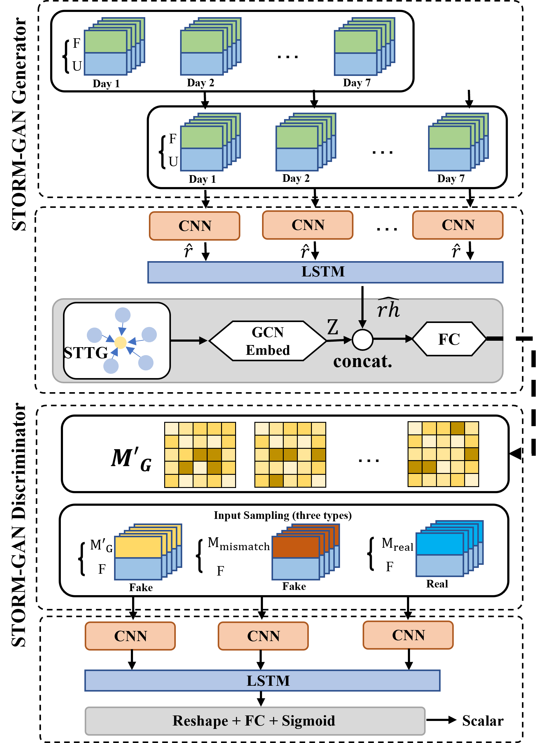
Figure 2: STORM-GAN architecture.

III-A STORM-GAN with Spatio-Temporal Task-based graph-embedding.

We now provide details for the three components in our proposed spatio-temporal meta-generative model: spatio-temporal generator, discriminator and spatio-temporal task-based graph embedding.

III-A1 Spatio-Temporal Generator

The spatio-temporal generator aims to generate human mobility responses while capturing the spatial patterns and temporal dependencies. The utilization of GAN structure allows known factors be learned as conditions and unknown factors be represented by latent noise which help the model to express these uncertainties (i.e., mobility response estimations may have some degree of variations). As shown in Fig. 2, the generator uses a stack of CNN and LSTM elements where CNN captures local spatial patterns and maintains the spatial representation (e.g., neighbor relationships), and LSTM is able to capture temporal trends in a given sequence. The generator takes a condition tensor $\textbf{F}\in\mathbb{R}^{l\times l\times k\times|T|}$ (we skip the batch dimension here for simplicity) and a latent code tensor $\textbf{U}\in\mathbb{R}^{l\times l\times u\times|T|}$, where $k$ is the number of conditions (e.g., policy, COVID statistics and contextual conditions), $u$ is the dimension of the noise vector for modeling the uncertainties, and $|T|$ is the length of a time period.

In the generator, denote the CNN output as $\hat{r}\in\mathbb{R}^{d\times|T|}$, where $d$ is the number of output features. Next, to capture temporal patterns and trends, $\hat{r}$ is fed into a LSTM layer, where the memory vector is concatenated to $\hat{r}$. Then, the output from the last timestamp of the LSTM layer $\hat{rh}$ will be concatenated with the graph embedding, and further passes through a fully connected layer to generate the final output. This $\hat{rh}$ is not yet the estimated mobility response $\textbf{M}^{\prime}_{G}$. For more robust estimation, the spatio-temporal generator additionally uses a proposed spatio-temporal task-based graph embedding to characterize task-level spatio-temporal features and potential dependency across multiple cities and their mobility patterns, as discussed in the next section.

III-A2 Spatio-Temporal Task-based Graph (STTG) Embedding

In real-world scenarios, spatial meta-learning tasks may have a very diverse distribution. For example, in our problem, tasks sampled from multiple cities can have significantly different human mobility patterns due to different urban contexts. Meanwhile, there may also exist underlying dependencies among cities due to traffic connections, geo-socio similarities, etc. Such spatial distribution of tasks, if properly utilized, would greatly enhance the performance of the learned meta-learning model.

To better model heterogeneity and dependency across spatio-temporal tasks, we propose a novel spatio-temporal task-based graph (STTG) to incorporate such information and facilitate the learning of transferable knowledge from related tasks. In the following part, we will first introduce the construction rules of STTG, and then discuss STTG-based embedding learning.

The STTG in our proposed STORM-GAN framework is a directed weighted graph $\mathcal{G}\left(\mathcal{V},\mathcal{E}\right)$, where nodes represent the spatial locations of tasks (e.g., cities) and edges (and weights) represent the relevance among spatial locations. The graph is attributed, meaning that the nodes are associated with attributes $f(\nu_{i})$ to describe the characteristics of each spatial location in the task space.

STTG can be defined in various ways depending on the underlying analysis goal and the network data used. In our particular application, we define each node $\nu_{i}$ as a major metropolitan area in the U.S, which contains features $f(\nu_{i})$ of the city such as the current stage of the pandemic. Each edge $e_{ij}$ connecting cities $\nu_{i}$ and $\nu_{j}$ indicates that there is geo-socio similarity between $\nu_{i}$ and $\nu_{j}$ in the pandemic, where the edge weight represents the strengths of such similarity. Depending on how “similarity” is measured, we can define the edge and weights differently. Examples of such measures may include the infection spreading between cities [10], correlation between cities’ mobility patterns, etc.

In this paper, we present two examples of STTG construction cases, although other definitions can be used with our method as well. In the first case, we define the edges and their weights based on physical reachability, i.e., the number of direct flights and driving distance between cities, with the assumptions that the COVID spreading is tightly related to traveling and that cities with stronger transportation connections tend to have more relevance in COVID situation. In the second case, we define the edges based on the similarity of historical mobility pattern distribution measured by the Kullback–Leibler (KL) divergence[11] between cities. We provide details on the STTG construction in Sec. IV-D, and show effectiveness in Sec. IV-E.

Next, we use the built STTG in the meta-training phase to help learn more useful knowledge across tasks. As Fig. 2 shows, during the training on generator, we first sample a task-specific 1-hop subgraph H for the corresponding node (a city) on the STTG. Then, we obtain a sub-graph embedding using Variational Graph Autoencoder (VGAE) which consists of Graph Convolution Neural network (GCNs) [12] by solving:

$$f(\textbf{X}^{L},A)=\alpha(\hat{D}^{-\frac{1}{2}}\hat{A}\hat{D}^{-\frac{1}{2}}\textbf{X}^{L-1}W^{L-1}),$$ (1)

where $A$ is the adjacency matrix, ${\hat{A}=A+I}$, ${I}$ is the identity matrix, ${\hat{D}}$ is the diagonal node degree matrix of ${\hat{A}}$, $\alpha(\cdot)$ is a activation function (e.g., ReLU), $X$ is the feature matrix of each node from the graph, and ${W}^{L-1}$ is a weight matrix for the ${L-1}^{th}$ layer. The encoder takes $A$ and $X$ as inputs and generates the latent variable $\mathcal{Z}$ as output. The decoder reconstructs a adjacency matrix defined by the inner product between latent variable $\mathcal{Z}$.

The graph feature representation $\mathcal{Z}$ is concatenated with the output $\hat{rh}$ (Fig. 2), and flows through a final fully connected layer in the spatio-temporal generator to achieve $\textbf{M}^{\prime}_{G}$. The new STTG and GCN-based embedding, being part of the generation process, will also help the meta-learner to incorporate the similarity and dependency among tasks.

III-A3 Spatio-Temporal Discriminator

Fig. 2 shows the structure of the discriminator, which takes a tensor of size $\mathbb{R}^{l\times l\times(k+1)\times|T|}$, where $k$ is the number of conditions (same as that for generator) and the added one dimension is for the mobility response layer.

To create training data for “fake” or “real” labels, the input tensors are created in three ways: (1) generated mobility $\textbf{M}^{\prime}_{G}$ concatenated with conditions; (2) real mobility $\textbf{M}_{real}$ concatenated with corresponding conditions; (3) conditions concatenated with mismatched real mobility $\textbf{M}_{mismatch}$. Only samples from the second combination are labeled “real”. Using these inputs, the discriminator learns to determine whether an input is “real” or “fake”.

STORM-GAN training on a single city is performed through adversarial configuration between the generator and discriminator. A min-max objective function is used to train ${G}$ and ${D}$ jointly by solving:

$$\small\begin{split}\mathcal{L}_{G,D}=\text{E}_{\textbf{M}\sim P_{data}}[\log D(\textbf{M},\textbf{F})]\\ +\,\text{E}_{\textbf{U}\sim P_{U}}[\log(1-D(G(\textbf{F},\textbf{U},{STTG}),\textbf{M}))]\end{split}$$ (2)

where $\mathcal{L}_{G,D}$ is the binary cross-entropy loss.

III-B STORM-GAN Training and Testing

III-B1 MAML-based Outer Loop Updates

As defined in Sec. I, our goal is to learn the shared knowledge or initialization across tasks drawn from multiple cities. To transfer the structural knowledge from graph and spatio-temporal knowledge from mobility data in multiple cities, we adopt the model-agnostic meta-learning (MAML) framework to learn the meta parameter $\theta_{D}$ and $\theta_{G}$, specifically in our case for all spatio-temporal tasks. The learned initialization is expected to contain common knowledge that can be fast-adapted to new tasks. With MAML, we sample a batch of tasks in each step, where each task $\mathcal{T}_{i}$ consists of (F, M) and their corresponding one-hop subgraph in STTG. The general optimization formulation is as follows. Given a set of tasks $\left\{\mathcal{T}_{1},\mathcal{T}_{2},...\right\}$ drawn from a task distribution $\mathit{p\left(\mathcal{T}\right)}$, where each task $\mathit{\mathcal{T}_{i}}\sim p(\mathcal{T})$ consists of a training and a test set $\{\mathit{\mathcal{D}_{i}^{train}},\mathit{\mathcal{D}_{i}^{test}}\}$, we optimize the $G$ and $D$ with parameters $\theta_{G}$ and $\theta_{D}$ to minimize the expected empirical loss across all tasks during meta-training. The meta-update rules are given by:

$$\theta_{D}=\theta_{D}-\beta\nabla_{\theta_{D}}\mathcal{L}_{G,D}(f_{\theta^{\prime}_{D}})$$ (3)

$$\theta_{G}=\theta_{G}-\beta\nabla_{\theta_{G}}\mathcal{L}_{G,D}(f_{\theta^{\prime}_{G}})$$ (4)

where $\beta$ is the learning rate for meta-update, and $\theta^{\prime}_{G}$ and $\theta^{\prime}_{D}$ represent temporary task-specific parameters. Following the recommendation in [8], we use the first-order MAML for meta-weight update.

III-B2 STORM-GAN Inner Loop Updates

The detailed meta-training procedure is shown in Alg. 1. The training of discriminator uses the three types of combinations: ($\textbf{M}^{\prime}_{G}$, F), ($\textbf{M}_{real}$, F) and ($\textbf{M}_{mismatch}$, F). Denote $\alpha$ as the learning rate of discriminator, $\theta^{\prime}_{D}$ as the parameters of discriminator, the loss function and the update rule of $D$ are shown in Eq. (5) and Eq. (6), respectively.

$$f_{D}= -\frac{1}{m}\sum_{i=1}^{m}\bigg{(}\log(1-D((\textbf{M}^{\prime}_{G})^{i},\textbf{F}^{i}))+\log(D(\textbf{M}^{i}_{real},\textbf{F}^{i}))$$ (5)

$$+\log(1-D(\textbf{M}^{i}_{mismatch},\textbf{F}^{i}))\bigg{)}$$

$$\small\theta^{\prime}_{D}=\theta^{\prime}_{D}-\alpha\nabla f_{D}(\theta^{\prime}_{D})$$ (6)

where $m$ is the total number of samples in a batch, and index $i$ refers to the $i^{th}$ sample. Denote $\theta^{\prime}_{G}$ as the parameters in $G$, we have the loss function and update rule of $G$ as:

$$f_{G} =\frac{1}{m}\sum_{i=1}^{m}\bigg{(}\log(1-D((\textbf{M}^{\prime}_{G})^{i},\textbf{F}^{i}))\bigg{)}$$ (7)

$$=\frac{1}{m}\sum_{i=1}^{m}\bigg{(}\log(1-D(G(\textbf{F}_{i},\textbf{U}_{i},{STTG}),\textbf{F}^{i}))\bigg{)}$$

$$\small\theta^{\prime}_{G}=\theta^{\prime}_{G}+\alpha\nabla f_{G}(\theta^{\prime}_{G})$$ (8)

III-B3 STORM-GAN Adaptation on New Tasks

During the model adaptation phase (e.g., updating the optimal initialization for a new task from a new city), we first copy $\theta_{G}$ and $\theta_{D}$ from the meta-training phase as the initialization for fast-adaptation, and then use training samples from the new task to perform STORM-GAN for updating the meta-parameter $\theta_{D}$ and $\theta_{G}$. Finally, the updated model outputs the estimated mobility using testing samples. The tasks used for meta-testing adaptation are held out from meta-training.

0:   

$\bullet$ Set of training cities $\textbf{T}_{\text{train}}$; set of testing cities $\textbf{T}_{\text{test}}$

$\bullet$ Conditions F, mobility $\textbf{M}_{\text{real}}$, a STTG $\mathcal{G}$

$\bullet$ Inner learning rate $\alpha$; outer learning rate $\beta$; number of epochs $epoch$

0:  $\theta_{G}$, $\theta_{G}$, estimated mobility $M^{\prime}_{G}$ for $\textbf{T}_{\text{test}}$

{# Meta-learning on training cities}

1:  G = initG(); D = initD()

2:  Randomly initialize meta $\theta_{G}$, $\theta_{G}$

3:  for $e$ = 1 to $epoch$ do

4:     Sample a batch of $\mathcal{T}$ from $\textbf{T}_{\text{train}}$

5:     Sample the subgragh H of $\mathcal{T}$ from $\mathcal{G}$

6:     for $\mathcal{T}_{i}$ in $\{\textbf{F},\textbf{M}_{\text{real}},$H$\}$ do

7:        Sample a set of disjoint $\mathit{\mathcal{D}_{i}^{train}}$, $\mathit{\mathcal{D}_{i}^{test}}$

8:        Generate graph embedding E of H

9:        $\textbf{M}^{\prime}_{G}$ = G(F, E, $rand$($P_{\textbf{U}}$))

10:        Update D using $\mathit{\mathcal{D}_{i}^{train}}$ by Eqs. (5) and (6)

11:        Update G using $\mathit{\mathcal{D}_{i}^{train}}$ by Eqs. (7) and (8)

12:        Evaluate estimation loss using $\mathit{\mathcal{D}_{i}^{test}}$ by Eq. (2)

13:     end for

14:     Update $\theta_{D}$ and $\theta_{G}$ by Eq. (3) and Eq. (4)

15:  end for

16:  Return $\theta_{G}$, $\theta_{D}$

{# Fast-adaptation on testing cities}

17:  Sample batch of testing tasks $\mathcal{T}$ from $\textbf{T}_{\text{test}}$

18:  for $\mathcal{T}_{i}$ in $\{\textbf{F},\textbf{M}_{\text{real}},$H$\}$ do

19:     Sample a disjoint $\mathit{\mathcal{D}_{i}^{train}}$, $\mathit{\mathcal{D}_{i}^{test}}$ from $\textbf{T}_{\text{test}}$

20:     Generate graph embedding E of H

21:     Copy $\theta_{G}$, $\theta_{D}$

22:     Evaluate performance by Eq. (2) using $\mathit{\mathcal{D}_{i}^{train}}$

23:     Update G through Eqs. (7) and (8)

24:     Estimate $\textbf{M}^{\prime}_{G}$ using updated G and $\mathit{\mathcal{D}_{i}^{test}}$

25:  end for

Algorithm 1 STORM-GAN Training and Testing

IV Evaluation

IV-A Dataset Description

Data Sources. We elaborate four types of data as described in Def. 3 & Def. 4 (pandemic, contextual, policy, and mobility). They are collected from Centers for Disease Control and Prevention [13], Census Bureau [14], the date of disease prevention policies were collected from the corresponding city government website news, and SafeGraph [15], respectively. SafeGraph provides free access to data for academic purposes with upon request and all the other data are publicly available.

Data Granularity. The original POI dataset from SafeGraph is obtained by collecting the location from cell phone records with latitude and longitude information. Then, the location information is used to determine the visits to POIs [15]. The POI visit counts data is in point data format. Fig. 3 illustrates the discretization of one city, where we sum the total POI visit counts that fall into each grid cell, and use this aggregated visit counts value to represents the human mobility responses of each grid cell.

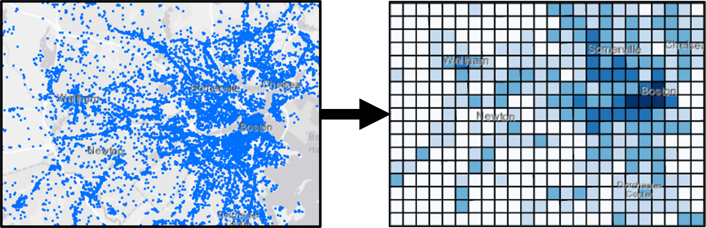
Figure 3: POI visit counts data pre-processing.

Data Pre-processing. To construct the list of conditions for our input, for each grid cell, we preprocess data collected from different sources with different geographic units. We first adopt a commonly used space-partitioning method to segment each spatial domain into grid cells of size of 1km $\times$ 1km, and segment all mobility related conditions using the same grid cells. Then, each spatial region (or unit spatial window) we used to create a data sample is a $10\times 10$ spatial window on the grid. For each grid cell, the value of human mobility response is the total number of POI visit counts in a day. Note that some conditions are re-scaled during this process. For example, population and median household income data are collected at the census tract level, and we linearly re-scaled the data using the corresponding area ratios between the area of the original census tract polygon and the proposed $10\times 10$ grid cells. Similarly, COVID-19 statistics and policy data are collected at the county level. We assign each grid cell with the corresponding data on which county it belongs.

Training Data Description. We collect the mobility related datasets from six cities. The dataset spans over six cities in different states located from the west coast, midwest to the east coast (i.e., Boston, Chicago, Houston, Iowa City, Los Angeles, and NYC). The list of cities also covers regions from large metropolitan areas to less populous places. Detailed statistics of these datasets (e.g., number of POIs, number of cells covered for each city) are listed in Table I and Table II. The duration of data is from 02/24/2020 to 10/25/2020, covering 35 weeks in total. As discussed in Methodology section, the data is segmented into a spatio-temporal distribution of tasks, where each task contains one single city for five consecutive weeks (no mutual overlaps among tasks). The candidate methods are trained on five cities (meta-training) with one left out as the new city for meta-testing. Adaptation on test cities is performed with data samples from the most recent two weeks (out of 35 weeks in total). Overall, we have 35 spatio-temporal estimation tasks in total. For methods with meta-learning, 80% of data in each task is used for meta-training, and the rest for testing (Def. 7).

TABLE I: Detailed data statistics.

City	Time Span (M/D/Y)	POIs	Size
Boston	02/24/2020 -10/25/2020 35 Weeks	26054	37 $\times$ 48
NYC		133520	58 $\times$ 72
LA		86721	52 $\times$ 64
Chicago		47356	50 $\times$ 40
Houston		37315	50 $\times$ 60
Iowa City		1401	20 $\times$ 32

TABLE II: Average number of POI visit counts per grid cell

City	Boston	NYC	LA	Chicago	Houston	Iowa City
POI Counts	28	64	52	30	24	6

IV-B Evaluation Metrics

We evaluate the performance of STORM-GAN by using the following measures: mean absolute error (MAE) and rooted mean square error (RMSE).

$$\small\begin{split}MAE=\frac{1}{n}\sum_{i=0}^{n}\left|M_{G}-\hat{M_{G}}\right|\end{split}$$ (9)

$$\small\begin{split}RMSE=\sqrt{\frac{1}{n}\sum_{i=1}^{n}\left(M_{G}-\hat{M_{G}}\right)^{2}}\end{split}$$ (10)

where $M_{G}$ is the real mobility response and $\hat{M_{G}}$ is the generated mobility response values by candidate approach. Since model generates the spatial unit windows multiple times for each grid cell during estimation, the outputs of generator are averaged before comparing with the ground truth.

To evaluate the model performance of learning the data distribution, we calculate the KL divergence to indicate the similarity between the learned human mobility responses distribution $\hat{\textbf{P}}$ and real human mobility responses distribution P on different bin sizes. The KL divergence is defined as follow:

$$\begin{split}\mathbf{D_{K}{}_{L}}(P||\hat{P})=\sum_{i=1}^{N}P(M^{\prime}_{G})log(\frac{P(M^{\prime}_{G})}{\hat{P}({M}_{real})})\end{split}$$ (11)

IV-C Baseline Methods

We compare our proposed method with the following baseline methods, and fine-tune each method using Houston and Iowa City as testing cities respectively.

• HA: Historical Average. The average of human mobility responses calculated using observed values from the same location in the past two weeks (same weekday).

• Spatial smoothing with neighborhood regions [16]. This method uses the mobility response values in a local $3\times 3$ window to compute a mean as the estimated value. The values for smoothing are from the same weekday in the most recent week.

• Ridge [17]. We use ridge regression with the same input features and mobility responses.

• cGAN [2]. A conditional GAN where the generator and discriminator use three fully-connected layers (no layer structure to learn spatial or temporal patterns).

• COVID-GAN [3]: COVID-GAN has the same structure as the above cGAN, and it adds a correction layer, which is used to add constraints based on policy to refine the results.

• MAML-DAWSON [5]: An optimization-based meta-learning approach using MAML. As DAWSON originally works on music generation tasks, we modify its inner structure with a regression-focused conditional GAN.

• MetaST [6]: MetaST fuses CNN, LSTM and attention mechanism to predict urban traffic volume through MAML framework.

IV-D STTG Construction Examples

In this section, we provide two different STTG construction scenarios to evaluate the effectiveness of graph embedding in human mobility estimation.

Scenario 1 (S1). We assume that cities of similar sizes, socio-economic environment, and land-use design may share similar human mobility pattern that could help the estimation of new cities. To build the graph $\mathcal{G}_{s1}\left(\mathcal{V},\mathcal{E}\right)$, we enumerate major metropolitan cities from every region in U.S., and define each city as a node $\nu_{i}$. Next, we extract human mobility maps for all the cities from a same date, and calculate the pairwise distribution similarity score between cities using KL-divergence. The KL-divergence indicates the strength of human mobility correlation. Each edge is added if the correlation is $\leqq$ 0.5, and is weighted by the correlation. $\mathcal{G}_{s1}$ contains 55 nodes and 682 edges. Node attribute store the outbreak stage of COVID-19. Each stage value is in $\{1,2,3\}$, where a smaller value means earlier in COVID-19 outbreak. The stage value is assigned based on the month when an exponential growth is first appeared.

Scenario 2 (S2). Intuitively, urban environment increases the chance of infection as people move around and interact with others and the environment. As a hub for migration and travel, urban areas may quickly spread infections to nearby places through short-distance travel, and to major cities through connection flights.

To construct ${S2}$, similar to ${S1}$, we enumerate major metropolitan areas in U.S, and define a graph $\mathcal{G}_{s2}\left(\mathcal{V},\mathcal{E}\right)$ to represent the relationships of these cities. We divide the nodes $\mathcal{V}$ into two categories: the hub nodes $\mathcal{V}^{h}$ are major cities with more than 100 airlines; the second-tier nodes $\mathcal{V}^{s}$ are cities with more than 35 but less than 100 airlines. Moreover, each directed edge $\nu_{i}\to\nu_{j}\in\mathcal{E}$ is added if its two nodes are: (1) both major cities that have direct flights; or (2) within a spatial proximity threshold (500 km in this paper). Our graph contains 69 nodes and 776 edges.

The graph is then weighted by spatio-temporal attributes associated with nodes and edges. Edge attributes contain the number of directed flights between the cities and their geographic distance. Node attributes store the sum of flights from connected edges as well as the outbreak stage of COVID-19 which is the same as scenario 1. Fig. 4 shows an illustration example of our ${S2}$ which is a 1-hop subgraph for Kansas City, a second-tier city by the above-mentioned classification. Major cities that have direct flights to Kansas City (e.g., Denver, Atlanta, Minneapolis) and second-tier cities (e.g., Oklahoma, Omaha) within the spatial proximity threshold are shown on the subgraph.

We use both of the two STTG definitions with our STORM-GAN (namely, STORM-GAN($S1$) and STORM-GAN($S2$)) to evaluate its performance in the next subsection.

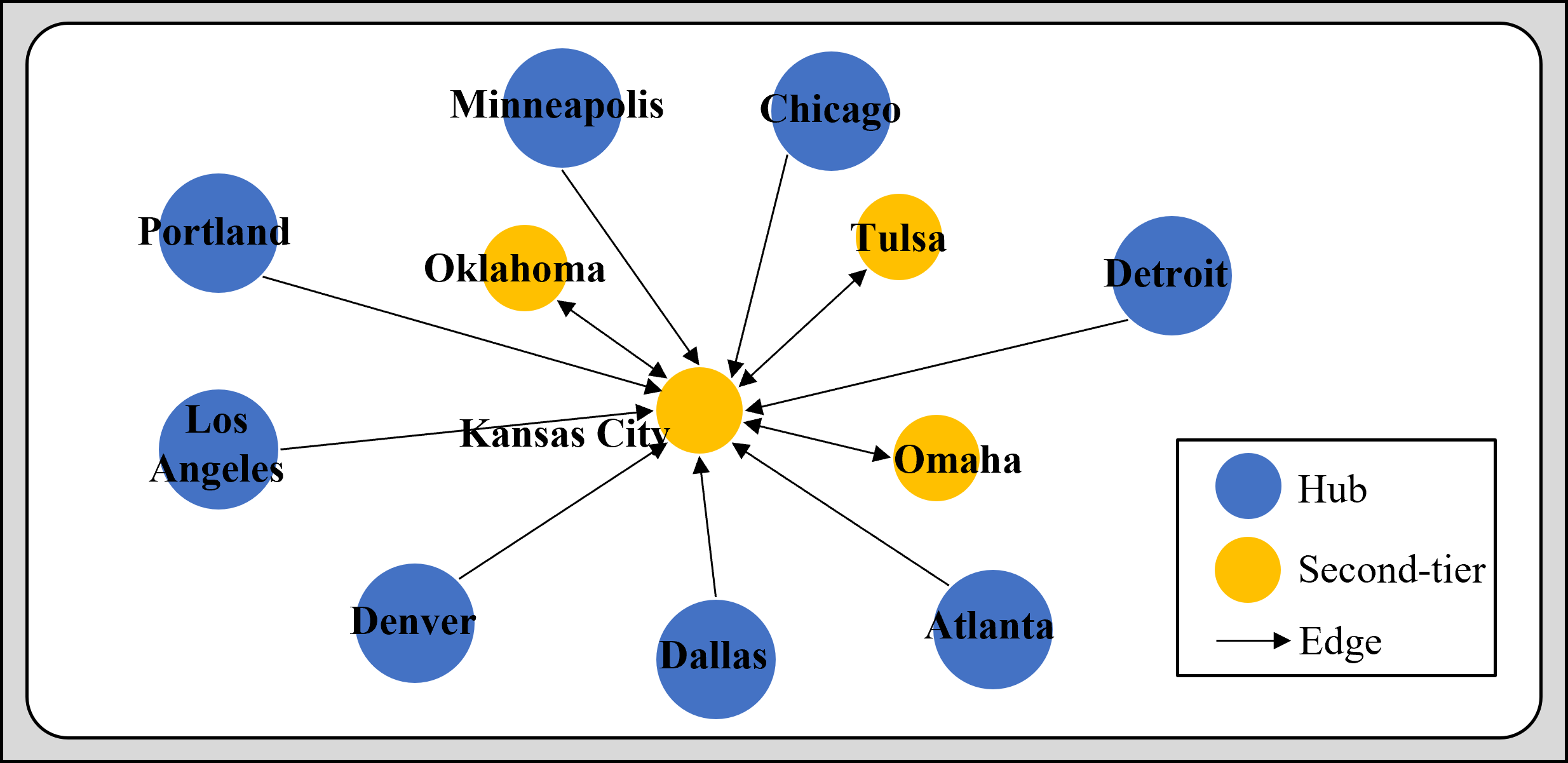
Figure 4: Subgraph of a node in STTG S2.

IV-E Estimation Quality Evaluation

The benefit of meta-learning is that the model can quickly update the model parameters, and generate good results on a new task by seeing a small fraction of new data. During the adaptation phase, we evaluate the performance of the candidate methods on the two test cities (i.e., Houston and Iowa City) using their last two weeks (Monday to Sunday) of data. The length of a time period we use is 7-day since human mobility pattern is influenced by strong weekly periodicity. For each testing city and week, we use 2 consecutive weeks of data ahead of the week for adaptation, and then use the parameters to generate the next 7-day (one week) human mobility responses.

TABLE III: Human mobility responses estimation by candidate methods for Houston

	RMSE							MAE
Model	Mon	Tues	Wed	Thu	Fri	Sat	Sun	Mon	Tues	Wed	Thu	Fri	Sat	Sun
HA	194.8	193.2	193.5	196.3	193.6	194.5	195.1	81.2	80.9	80.4	80.8	79.6	81.3	81.2
Smoothing	150.9	168.1	169.2	177.1	187.3	202.4	162.1	82.3	90.2	90.4	94.6	100.1	99.8	104.2
cGAN	278.2	283.4	284.6	279.5	286.3	286.1	286.2	118.7	122.4	125.3	120.6	128.3	130.6	129.3
Ridge	189.4	192.1	182.3	181.5	187.3	188.6	195.7	95.8	99.5	101.9	95.3	99.4	98.1	95.2
COVID-GAN	171.5	175.6	174.3	172.2	176.4	171.8	170.6	75.1	80.1	73.2	77.1	80.5	81.7	82.8
MAML-DAWSON	169.5	169.7	166.1	168.9	164.6	166.7	168.1	68.3	67.4	70.3	69.4	68.2	75.5	78.2
MetaST	170.2	171.4	173.8	170.6	169.5	170.3	169.4	72.8	76.1	71.5	74.2	72.9	80.2	81.3
STROM-GAN (${S1}$)	151.2	150.5	149.3	162.9	163.9	164.2	167.2	66.7	66.4	64.7	63.1	70.4	71.8	72.2
STORM-GAN (${S2}$)	145.1	142.6	141.9	141.6	152.5	156.7	160.2	61.7	60.4	59.3	53.8	58.4	64.2	67.2

TABLE IV: Human mobility responses estimation by candidate methods for Iowa City

	RMSE							MAE
Model	Mon	Tues	Wed	Thu	Fri	Sat	Sun	Mon	Tues	Wed	Thu	Fri	Sat	Sun
HA	22.2	23.1	21.3	24.2	22.3	25.2	26.5	13.4	13.1	15.2	12.6	14.2	16.1	13.2
Smoothing	18.4	16.3	18.6	21.7	18.3	19.2	19.5	11.2	10.3	10.6	9.1	11.6	9.2	11.6
cGAN	34.3	33.7	34.8	36.5	32.8	31.2	34.4	21.1	19.5	21.3	18.7	17.8	19.9	20.3
Ridge	20.6	22.3	21.1	20.5	19.8	19.2	20.1	12.4	11.6	13.3	13.6	12.2	13.5	12.2
COVID-GAN	17.1	17.3	16.6	16.3	15.2	14.3	15.6	11.3	10.7	13.1	12.3	14.7	13.8	13.3
MAML-DAWSON	16.5	17.6	17.7	15.2	15.3	13.6	13.4	10.3	11.6	10.1	9.5	8.1	10.9	9.2
MetaST	17.1	17.4	17.8	17.6	16.5	16.3	16.1	10.8	10.6	10.4	10.5	9.9	10.1	9.7
STROM-GAN (${S1}$)	15.8	16.2	16.1	15.8	15.9	15.4	14.3	8.9	9.6	9.9	10.2	9.1	9.3	9.3
STORM-GAN (${S2}$)	14.1	15.6	14.9	14.4	14.2	13.6	13.3	8.2	7.4	9.1	8.3	7.8	9.1	8.5

Performance comparison of proposed STORM-GAN and other candidate methods. Tables III and IV show the results of the candidate methods obtained using Houston and Iowa City as the testing city, respectively. We apply $S1$ and $S2$ graph construction scenarios on STROM-GAN, respectively. The evaluation results show that both STORM-GAN scenarios overall achieve the lowest RMSE and MAE for each day in the week, with major improvements from 91.7$\%$ to 17.6$\%$. It is interesting to observe that historical average and spatial smoothing methods perform better than the basic cGAN, which to some degree shows the spatio-temporal auto-correlation effects. However, these methods can mainly estimate a rough base but are limited in capturing complex spatio-temporal relationships between features and mobility responses. Comparing to COVID-GAN and MAML-DAWSON, our model outperforms COVID-GAN by 20.5% (RMSE) and 23.5% (MAE) on average, and MAML-DAWSON by 15.1% (RMSE) and 23.4% (MSE). The results show that the design of spatio-temporal architecture (i.e., CNN and LSTM substructures and the STTG graph) and meta-learning adaptation can significantly improve the solution quality. Furthermore, our model achieves 14.7% (RMSE) and 15.2% (MSE) better than MetaST, demonstrating that task-based graph embedding can contribute to model performance by learning the inter-task similarities. We evaluate the model performance on less populous areas using Iowa City as testing city, the POI numbers and city size of Iowa City are significantly smaller than large metropolitan areas according to Tables I and II. As Table IV shows, the improvements are relatively smaller due to smaller number of POI visit counts in less populated city. However, both STORM-GAN scenarios still achieve the lowest errors in all of the testing days.

We calculate the KL-divergence using results from Houston and Iowa City (Fig. 5). The X-axis represents the number of equal-size bins used to discretize the value needed for the computation, and the Y-axis shows the KL divergence values. A lower KL divergence value means the result better matches the real distribution. As shown in Fig. 5, STORM-GAN achieves lowest KL-divergence compare to the baseline methods consistently for all numbers of bins.

Impact of STTG choice: Our results show that both of the two STTG constructed can significantly improve the performance of STORM-GAN in Houston and Iowa City. This proves that the spatio-temporal task-graph embedding design is effective and robust, rather than tailored for a specific STTG definition. Between the two choices, $S2$ generally achieves better performance as it uses more information that are directly related to the spreading of COVID-19.

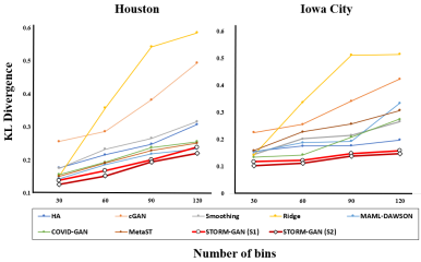
Figure 5: Kullback-Leibler divergence.

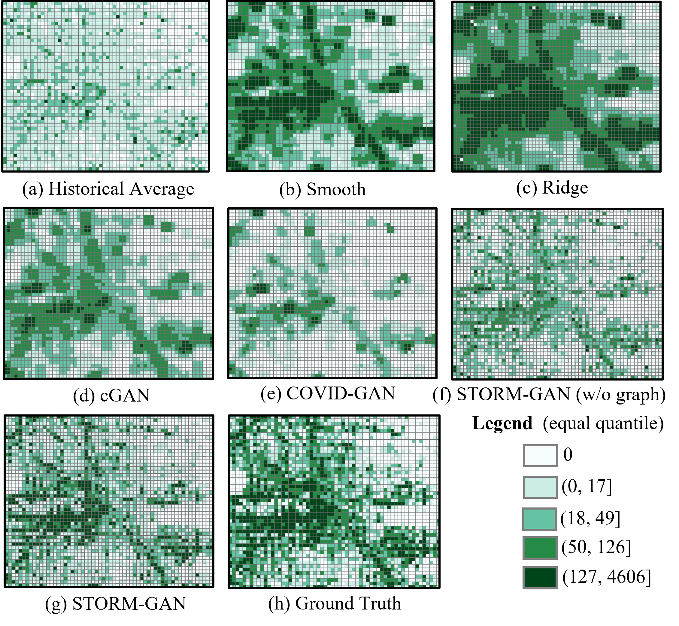
Figure 6: Mobility estimation results of the Houston study area.

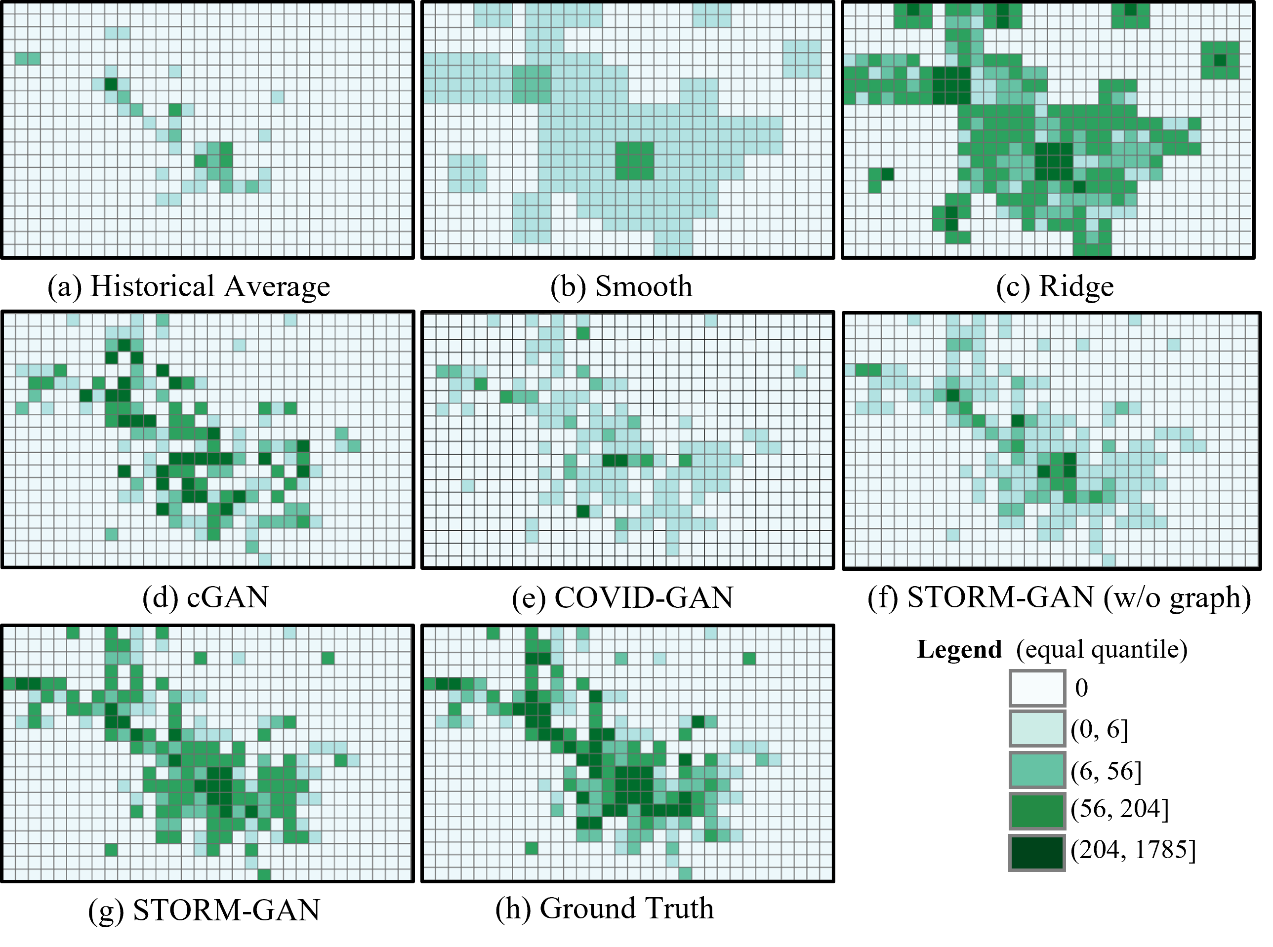
Figure 7: Mobility estimation results of the Iowa City study area.

Ablation Study. We study the effect of different components proposed in our method using Houston as the testing city on one day (Monday).

• Base: Baseline conditional GAN.

• Base + Spatial (S): Equivalent to COVID-GAN, which has a correction layer to add policy constraints, but purely a spatial model.

• Base + Spatio-Temporal (ST) + Meta: Proposed STORM-GAN with spatio-temporal meta-learning, but without the STTG graph.

• Base + ST + Meta + Graph(S2): Complete STORM-GAN.

TABLE V: Comparison among STORM-GAN variations

Method	RMSE	MAE
Base	202.2	80.6
Base + S	171.5	75.1
Base + ST + Meta	149.8	67.6
Base + ST + Meta + Graph (${S2}$)	145.1	61.7

Table V shows the estimation performance of STORM-GAN and its variants. First, the base + spatial (S) achieves a lower RMSE and MAE (a reduction of 15.3% and 15.2%, respectively) compared to cGAN, showing the effectiveness of the correction layer from COVID-GAN. Next, we can see that the addition of spatio-temporal meta-learning further reduces RMSE and MAE by 12.7% and 10%, respectively. This result demonstrates that CNN, LSTM and meta-learning can better capture the complex spatio-temporal relationships across multiple cities. Finally, the complete STROM-GAN achieves the lowest RMSE and MAE with the sptaio-temporal task-based graph.

Visualization. We compare the solution quality of seven candidate approaches through map visualization. Fig. 6 and Fig. 7 (a) to (f) show the results of baseline methods, and (g), (h) show the STORM-GAN (${S2}$) and ground truth. The results show the full Houston and Iowa City study areas for a day in the data. Here STORM-GAN generates fine-scale mobility values that are closer to the ground truth. As we can see, the mobility pattern generated by the STORM-GAN can capture the spatial pattern of human mobility responses better than other baselines. The reason may be that similar functionality zones at different cities may have similar mobility patterns. The meta-learning framework successfully learns this shared knowledge from training tasks. Moreover, the utilization of CNN and LSTM helps capture the spatio-temporal correlation from region to region.

V Other Related Work

Deep Learning for Spatio-Temporal Prediction. There have been many deep learning based techniques developed for spatiotemporal data. For example, LSTM were widely used in traffic accident prediction [18] due to its capability in capturing spatio-temporal correlation and thus provide good prediction results. Geospatial object mapping [19], taxi driver behavior imitation [20], taxi demand [21], travel time estimation [22], etc, they all combine the deep learning model with spatio-temporal perspective in their model design and obtain good performance. Most of these techniques typically are stationary predictors (i.e., same result from two runs on same data) rather than generative models, and they do not consider the unknown factors in prediction, and their performance relies on large data sets. Besides, they do not leverage domain knowledge based constraints to assist learning (e.g., cGAN [3, 2]).

Meta-Learning. Meta-learning learns new tasks quickly and effectively with a few examples. Existing optimization-based meta-learning algorithms such as MAML [8] and Reptile [23] rely on optimization through gradient descent, and both are compatible with any model. Recently, the idea of optimization-based meta-learning has been applied to many domains including classification and reinforcement learning. However, there only are a few work address the spatial and temporal problems simultaneously. In traffic prediction, a recent work [7] focuses on knowledge transfer in a single city, which only deals with temporal tasks with no spatial-based tasks. [24] proposes a transfer learning framework for traffic prediction through learning region matching function. Another work [6] which is based on multiple cities does not consider temporal patterns and dynamic scenarios.

Mobility Estimation. There have been many studies [1, 25, 26] exploring the interplay between human mobility responses, social distancing policies, and transmission dynamics in response to the COVID-19 pandemic. A US mobility change map was created in [25] to increase risk awareness of the public and to visualize dynamic changes in mobility as COVID-19 situation and policy evolves. These studies are timely in showing the important role played by mobility in the spread of COVID-19, but they do not address the challenges in real-world mobility estimation/simulation (e.g., effects of unknown, uncertain, and random factors), and they analyze the mobility changes in city or country scale. A study [27] simulated the human mobility which allows policymakers to inspect mobility changes under different policies. But this approach utilizes a traditional epidemiological model, and does not transfer the simulation from city to city by shared knowledge. However, these studies have not explored the potential use of deep learning based generative models and meta-learning to assist the estimation.

VI Conclusions

We made the first attempt to tackle the human mobility estimation problem through a spatio-temporal meta-generative framework. Specifically, we proposed a STORM-GAN model to capture complex spatio-temporal patterns using a set of social and policy conditions related to COVID-19. We also proposed a novel spatio-temporal task-based graph (STTG) to represent the spatio-temporal relationships among cities, with a graph convolution network to learn embeddings of its subgraph for cross-task learning enhancements. Finally, STORM-GAN utilized the meta-learning paradigm to learn shared-knowledge from a spatio-temporal distribution of estimation tasks and can quickly adapt to new tasks (e.g., new cities). The experiment results showed that our proposed approach can significantly improve the estimation performance compared to baselines. The model can assist policymakers to better understand the dynamic mobility pattern changes under different social and policy conditions, and can potentially be leveraged to inform decisions in resource allocation and provisioning, event planning, response management, etc.

References

- [1] M. U. Kraemer, C.-H. Yang, B. Gutierrez, C.-H. Wu, B. Klein, D. M. Pigott, L. Du Plessis, N. R. Faria, R. Li, W. P. Hanage et al., “The effect of human mobility and control measures on the covid-19 epidemic in china,” Science, vol. 368, no. 6490, pp. 493–497, 2020.
- [2] Y. Zhang, Y. Li, X. Zhou, X. Kong, and J. Luo, “Trafficgan: Off-deployment traffic estimation with traffic generative adversarial networks,” in 2019 IEEE International Conference on Data Mining (ICDM). IEEE, 2019, pp. 1474–1479.
- [3] H. Bao, X. Zhou, Y. Zhang, Y. Li, and Y. Xie, “Covid-gan: Estimating human mobility responses to covid-19 pandemic through spatio-temporal conditional generative adversarial networks,” in Proceedings of the 28th International Conference on Advances in Geographic Information Systems, ser. SIGSPATIAL ’20. New York, NY, USA: Association for Computing Machinery, 2020, p. 273–282. [Online]. Available: https://doi.org/10.1145/3397536.3422261
- [4] R. Jiang, X. Song, Z. Fan, T. Xia, Z. Wang, Q. Chen, Z. Cai, and R. Shibasaki, “Transfer urban human mobility via poi embedding over multiple cities,” ACM Transactions on Data Science, vol. 2, no. 1, pp. 1–26, 2021.
- [5] W. Liang, Z. Liu, and C. Liu, “Dawson: A domain adaptive few shot generation framework,” arXiv preprint arXiv:2001.00576, 2020.
- [6] H. Yao, Y. Liu, Y. Wei, X. Tang, and Z. Li, “Learning from multiple cities: A meta-learning approach for spatial-temporal prediction,” in The World Wide Web Conference, 2019, pp. 2181–2191.
- [7] Y. Zhang, Y. Li, X. Zhou, and J. Luo, “cst-ml: Continuous spatial-temporal meta-learning for traffic dynamics prediction,” in 2020 IEEE International Conference on Data Mining (ICDM). IEEE, 2020, pp. 1418–1423.
- [8] C. Finn, K. Xu, and S. Levine, “Probabilistic model-agnostic meta-learning,” Advances in neural information processing systems, vol. 31, 2018.
- [9] Y. Jiang, H. Chen, M. Loew, and H. Ko, “Covid-19 ct image synthesis with a conditional generative adversarial network,” IEEE Journal of Biomedical and Health Informatics, vol. 25, no. 2, pp. 441–452, 2020.
- [10] Y. Kang, S. Gao, Y. Liang, M. Li, J. Rao, and J. Kruse, “Multiscale dynamic human mobility flow dataset in the us during the covid-19 epidemic,” Scientific data, vol. 7, no. 1, pp. 1–13, 2020.
- [11] S. Kullback, Information theory and statistics. Courier Corporation, 1997.
- [12] M. Chen, Z. Wei, Z. Huang, B. Ding, and Y. Li, “Simple and deep graph convolutional networks,” in International Conference on Machine Learning. PMLR, 2020, pp. 1725–1735.
- [13] “Centers for disease control and prevention,” https://www.cdc.gov/, 2020.
- [14] “American community survey (acs),” https://www.census.gov/programs-surveys/acs, 2020.
- [15] “Safegraph,” https://www.safegraph.com/, 2020.
- [16] A. Getis, “A history of the concept of spatial autocorrelation: A geographer’s perspective,” Geographical analysis, vol. 40, no. 3, pp. 297–309, 2008.
- [17] R. W. Hoerl, “Ridge regression: a historical context,” Technometrics, vol. 62, no. 4, pp. 420–425, 2020.
- [18] Z. Yuan, X. Zhou, and T. Yang, “Hetero-convlstm: A deep learning approach to traffic accident prediction on heterogeneous spatio-temporal data,” in Proceedings of the 24th ACM SIGKDD International Conference on Knowledge Discovery & Data Mining, 2018, pp. 984–992.
- [19] Y. Xie, H. Bao, S. Shekhar, and J. Knight, “A timber framework for mining urban tree inventories using remote sensing datasets,” in 2018 IEEE International Conference on Data Mining (ICDM). IEEE, 2018, pp. 1344–1349.
- [20] X. Zhang, Y. Li, X. Zhou, and J. Luo, “Unveiling taxi drivers’ strategies via cgail: Conditional generative adversarial imitation learning,” in 2019 IEEE International Conference on Data Mining (ICDM). IEEE, 2019, pp. 1480–1485.
- [21] C. Zhang, F. Zhu, Y. Lv, P. Ye, and F.-Y. Wang, “Mlrnn: Taxi demand prediction based on multi-level deep learning and regional heterogeneity analysis,” IEEE Transactions on Intelligent Transportation Systems, 2021.
- [22] S. Xu, R. Zhang, W. Cheng, and J. Xu, “Mtlm: a multi-task learning model for travel time estimation,” GeoInformatica, pp. 1–17, 2020.
- [23] A. Nichol and J. Schulman, “Reptile: a scalable metalearning algorithm,” arXiv preprint arXiv:1803.02999, vol. 2, no. 3, p. 4, 2018.
- [24] L. Wang, X. Geng, X. Ma, F. Liu, and Q. Yang, “Cross-city transfer learning for deep spatio-temporal prediction,” arXiv preprint arXiv:1802.00386, 2018.
- [25] S. Gao, J. Rao, Y. Kang, Y. Liang, and J. Kruse, “Mapping county-level mobility pattern changes in the united states in response to covid-19,” SIGSPATIAL Special, vol. 12, no. 1, pp. 16–26, 2020.
- [26] M. Chinazzi, J. T. Davis, M. Ajelli, C. Gioannini, M. Litvinova, S. Merler, A. P. y Piontti, K. Mu, L. Rossi, K. Sun et al., “The effect of travel restrictions on the spread of the 2019 novel coronavirus (covid-19) outbreak,” Science, vol. 368, no. 6489, pp. 395–400, 2020.
- [27] S. Chang, M. L. Wilson, B. Lewis, Z. Mehrab, K. K. Dudakiya, E. Pierson, P. W. Koh, J. Gerardin, B. Redbird, D. Grusky et al., “Supporting covid-19 policy response with large-scale mobility-based modeling,” in Proceedings of the 27th ACM SIGKDD Conference on Knowledge Discovery & Data Mining, 2021, pp. 2632–2642.