Superconductivity in type II layered Weyl semi-metals

Abstract

Novel ”quasi two dimensional” typically layered (semi) metals offer a unique opportunity to control the density and even the topology of the electronic matter. In intercalated $MoTe_{2}$ type II Weyl semi - metal the tilt of the dispersion relation cones is so large that topologically of the Fermi surface is distinct from a more conventional type I. Superconductivity observed recently in this compound [Zhang et al, 2D Materials 9, 045027 (2022)] demonstrated two puzzling phenomena: the gate voltage has no impact on critical temperature, $T_{c},$ in wide range of density, while it is very sensitive to the inter - layer distance. The phonon theory of pairing in a layered Weyl material including the effects of Coulomb repulsion is constructed and explains the above two features in $MoTe_{2}$.  The first feature turns out to be a general one for any type II topological material, while the second reflects properties of the intercalated materials affecting the Coulomb screening.

I Introduction.

The 3D and 2D topological quantum materials, such as topological insulators and Weyl semi - metals (WSM), attracted much interests due to their rich physics and promising prospects for application in electronic and spinotronic devices. The band structure in the so called type I WSM like grapheneKatsnelson , is characterized by appearance linear dispersion relation (cones around several Dirac points) due to the band inversion. This is qualitatively distinct from conventional metals, semi - metals or semiconductors, in which bands are typically parabolic. In type-II WSM Soluyanov , the cones have such a strong tilt, $\kappa$, so that they exhibit a nearly flat band and the Fermi surface ”encircles” the Brillouin zone, Fig.1b, Fig.1c. It is topologically distinct from conventional ”pockets”, see Fig.1a. This in turn leads to exotic electronic properties different from both the those in both the conventional and in the type I WSM. Examples include the collapse of the Landau level spectrum in magnetoresistance Yu , and novel quantum oscillations Brien .

The type II topology of the Fermi surface was achieved in particular in transition metal dichalcogenides Wang . Very recently$MoTe_{2}$ layers intercalated by ionic liquid cations were studiedZhang22 . The tilt value was estimated to as high as $\kappa=1.3$ that places it firmly within the type II WSM class. The measurements included the Hall effect and the resistivity at low temperatures demonstrating appearance of superconductivity. They discovered two intriguing facts that are currently under discussion. First changing the gate voltage (chemical potential) surprisingly has no impact on critical temperature, $T_{c}$, in wide range of density of the electron gas. Second $T_{c}$ turned out to be very sensitive to the inter - layer distance $d$: it increases from $10.5A$ to $11.7A$, while the critical temperature jumps from $4.2K$ to $7K$. In the present paper we propose a theoretical explanation of these observations based on appropriate generalization of the conventional superconductivity theory applied to these materials.

Although early on unconventional mechanisms of superconductivity in WSM have been considered, accumulated experimental evidence points towards the conventional phonon mediated one DasSarma ; FuBerg ; frontiers . In  the previous paperRosenstein17 and a related workZyuzin a continuum theory of conventional superconductivity in WSM was developed. Magnetic response in the superconducting state was calculatedZyuzin Rosenstein18 . The model was too ”mesoscopic” to describe the type II phase since the global topology of the Brillouin zone was beyond the scope of the continuum approach. Therefore we go beyond the continuum model in the present paper by modeling a type II layered WSM using a tight binding approach. The in-plane electron liquid model is similarl to that of graphene oxideJian12 and other 2D WSM. It possesses a chiral symmetry between two Brave sublattices for all values of the tilt parameter $\kappa$, but lacks hexagonal symmetry. The second necessary additional feature is inclusion of Coulomb repulsion.

It turns out that the screened Coulomb repulsion significantly opposes the phonon mediated pairing. Consequently a detailed RPA theory of screening in a layered materialElliasson is applied. We calculate the superconducting critical temperature taking into consideration the modification of the Coulomb interaction due to the dielectric constant of intercalator material and the inter-layered spacing $d$. The Gorkov equations for the two sublattices system are solved without resorting to the mesoscopic approach. Moreover since screening of Coulomb repulsion plays a much more profound role in quasi 2D materials the pseudo-potential simplification developed by McMillanMcMillan is not valid.

Rest of the paper is organized as follows. In Section II the microscopic model of the layered WSM is described. The RPA calculation of both the intra- and inter - layer screening is presented. In Section III the Gorkov equations for the optical phonon mediated intra- layer pairing for a multiband system including the Coulomb repulsion is derived and solved numerically. In Section IV the phonon theory of pairing including the Coulomb repulsion for a layered material is applied to recent extensive experiments on $MoTe_{2}$. The effect of intercalation and density on superconductivity is studied. This explains the both remarkable features of $T_{c}$ observedZhang22 in $MoTe_{2}$. The last Section contains conclusions and discussion.

Figure 1: Two distict topologies of the Fermi surface in 2D. Topology of the 2D Brillouin zone is that of the surface of 3D torroid. On the left the “conventional” type I pocket is shown. In the ceter and on the right the type II topology is shown schematically. The filled states are in blue and envelop the torus. Despite the large difference in density of the two the Fermi surface properties like density of states are the same.

II A ”generic” lattice model of layered Weyl semi-metals

II.1 Intra- layer hopping

A great variety of tight binding models were used to describe Weyl (Dirac) semimetals in 2D. Historically the first was graphene (type I, $\kappa=0$) , in which electrons hope between the neighboring cites of the honeycomb lattice. We restrict the discussion to systems with the minimal two cones of opposite chirality and negligible spin orbit coupling. The two Dirac cones appear in graphene at $K$ and $K^{\prime}$ crystallographic points in BZ. Upon modification (more complicated molecules like graphene oxide, stress, intercalation) the hexagonal symmetry is lost, however a discrete chiral symmetry between two sublattices, denoted by $I=A,B$, ensures the WSM. The tilted type I and even type II (for which typically $\kappa>1$) crystals can be described by the same Hamiltonian with the tilt term added. This 2D model is extended to a layered system with inter - layer distance $d$. Physically the 2D WSM layers are separated by a dielectric material with inter - layer hopping neglected, so that they are coupled electromagnetically onlyElliasson .

The lateral atomic coordinates are still considered on the honeycomb lattice are $\mathbf{r}_{\mathbf{n}}=n_{1}\mathbf{a}_{1}+n_{2}\mathbf{a}_{2}$, where lattice vectors are:

$$\mathbf{a}_{1}=\frac{a}{2}\left(1,\sqrt{3}\right);\text{ }\mathbf{a}_{2}=\frac{a}{2}\left(1,-\sqrt{3}\right)\text{,}$$ (1)

despite the fact that hopping energies are different for jumps between nearest neighbors. Each site has three neighbors separated by $\mathbf{\delta}_{1}=\frac{1}{3}\left(\mathbf{a}_{1}-\mathbf{a}_{2}\right),\mathbf{\delta}_{2}=-\frac{1}{3}\left(2\mathbf{a}_{1}+\mathbf{a}_{2}\right)$ and $\mathbf{\delta}_{3}=\frac{1}{3}\left(\mathbf{a}_{1}+2\mathbf{a}_{2}\right)$, in different directions. The length of the lattice vectors $a$ will be taken as the length unit and we set $\hbar=1$. The hopping Hamiltonian including the tilt term isGoerbig ; Jian12 :

$$K=\frac{\sqrt{3}}{4}\sum\nolimits_{\mathbf{n}l}\left\{\gamma\left(\psi_{\mathbf{n}l}^{sA\dagger}\psi_{\mathbf{r}_{\mathbf{n}}+\mathbf{\delta}_{1},l}^{sB}+\psi_{\mathbf{n}l}^{sA\dagger}\psi_{\mathbf{r}_{\mathbf{n}}+\mathbf{\delta}_{2},l}^{sB}+t\psi_{\mathbf{n}l}^{sA\dagger}\psi_{\mathbf{r}_{\mathbf{n}}+\mathbf{\delta}_{3},l}^{sB}\right)+\mathrm{h.c.}-\kappa\psi_{\mathbf{n}l}^{sI\dagger}\psi_{\mathbf{r}_{\mathbf{n}}+\mathbf{a}_{1},l}^{sI}-\mu n_{\mathbf{n},l}\right\}\text{.}$$ (2)

Here an integer $l$ labels the layers. Operator $\psi_{\mathbf{n}l}^{sA\dagger}$ is the creation operators with spin $s=\uparrow,\downarrow$, while the density operator is defined as $n_{\mathbf{n}l}=\psi_{\mathbf{n}l}^{sI\dagger}\psi_{\mathbf{n}l}^{sI}$. The chemical potential is $\mu$, while $\gamma$ is the hopping energy for two neighbors at $\mathbf{\delta}_{1},\mathbf{\delta}_{2}$ . Since the the system does not possesses hexagonal symmetry (only the chiral one), the third jump has the different hoppingJian12 $t\gamma$. Dimensionless parameter $\kappa$ determines the tilt of the Dirac cones along the $\mathbf{a}_{1}$directionGoerbig . In the 2D Fourier space, $\psi_{\mathbf{n}l}^{sA}=N_{s}^{-2}\sum\nolimits_{\mathbf{k}}\psi_{\mathbf{k}l}^{sA}e^{-i\mathbf{k\cdot r}_{n}}$, one obtains for Hamiltonian

(for finite discrete reciprocal lattice $N_{s}\times N_{s}$):

$$K=N_{s}^{-2}\sum\nolimits_{\mathbf{k}l}\psi_{\mathbf{k}l}^{s\dagger}M_{\mathbf{k}}\psi_{\mathbf{k}l}^{s}.$$ (3)

Here $\mathbf{k}=\frac{k_{1}}{N_{s}}\mathbf{b}_{1}+\frac{k_{2}}{N_{s}}\mathbf{b}_{2}$ (reciprocal lattice vectors are given in Appendix A) and matrix $M_{\mathbf{k}}=d_{x}\sigma_{x}+d_{y}\sigma_{y}+d_{0}I$ in terms of Pauli matrices has components:

$$d_{x} = \frac{2t}{\sqrt{3}}\cos\left[\frac{2\pi}{3N_{s}}\left(k_{1}-k_{2}\right)\right]+\frac{4}{\sqrt{3}}\cos\left[\frac{\pi}{N_{s}}\left(k_{1}+k_{2}\right)\right]\cos\left[-\frac{\pi}{3N_{s}}\left(k_{1}-k_{2}\right)\right];$$ (4)

$$d_{y} = -\frac{2t}{\sqrt{3}}\sin\left[\frac{2\pi}{3N_{s}}\left(k_{1}-k_{2}\right)\right]+\frac{4}{\sqrt{3}}\cos\left[\frac{\pi}{N_{s}}\left(k_{1}+k_{2}\right)\right]\sin\left[\frac{\pi}{3N_{s}}\left(k_{1}-k_{2}\right)\right];$$

$$d_{0} = \frac{2}{\sqrt{3}}\left\{-\kappa\cos\left[\frac{2\pi}{N_{s}}k_{1}\right]-\mu\right\}\text{.}$$

Using $\gamma$ as our energy unit from now on, the free electrons part of the Matsubara action for Grassmanian fields $\psi_{\mathbf{k}ln}^{\ast sI}$ is:

$$S^{e}=\frac{1}{T}\sum\nolimits_{\mathbf{k}ln}\psi_{\mathbf{k}ln}^{\ast sI}\left\{\left(-i\omega_{n}+d_{\mathbf{k}}^{0}\right)\delta^{IJ}+\sigma_{i}^{IJ}d_{\mathbf{k}}^{i}\right\}\psi_{\mathbf{k}ln}^{sJ}\text{.}$$ (5)

where $\omega_{n}=\pi T\left(2n+1\right)$ is the Matsubara frequency. The Green Function of free electrons has the matrix form

$$g_{\mathbf{k}n}=\left\{\left(-i\omega_{n}+d_{\mathbf{k}}^{0}\right)I+\sigma_{i}d_{\mathbf{k}}^{i}\right\}^{-1}=\frac{\left(-i\omega_{n}+d_{\mathbf{k}}^{0}\right)I-\sigma_{i}d_{\mathbf{k}}^{i}}{\left(i\omega_{n}-d_{\mathbf{k}}^{0}\right)^{2}-d_{\mathbf{k}}^{x2}-d_{\mathbf{k}}^{y2}}\text{.}$$ (6)

Now we turn to the spectrum of this model.

Figure 2: The topological phase diagram of the Weyl semimetal at large tilt parameter ($\kappa=1.3$). Chemical potential (in units of $\gamma=500$ meV) is marked on each contour. The electron type I topology at low values of $\mu$ undergoes transition to the type II at $\mu=\mu_{c}^{1}=0.8$ meV. At yet larger $\mu>\mu_{c}^{2}=1.35$. the Fermi surface becomes again type I. This time the excitations are hole rather than electrons.

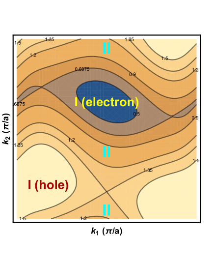
Figure 3: Dispersion relation of WSM with $\kappa=1.3$. The blue plane corresponds to chemical potentia l$\mu=0.8$ eV so that the Fermi surface has the type II topology.

II.2 The range of the topological type II phase at large $\kappa$

The spectrum of Hamiltonian of Eqs.(4) consists of two branches. The upper branch for $\mu=0.9eV$ is given in Fig. 2. The lower branch for a reasonable choice of parameters appropriate to $MoTe_{2}$ is significantly below the Fermi surface and is not plotted. Blue regions represent the filled electron states. One observes a ”river” from one boundary to the other of the Brillouin zone (in coordinates $k_{1}$ and $k_{2}$, in terms of the original $k_{x},k_{y}$ it is a rhomb) characteristic to type II Fermi surface. Topologically this is akin to Fig.1b.

In Fig. 3 the Fermi surfaces in a wide range of densities $n=7.\times 10^{13}-4.5\times 10^{14}cm^{-2}$ are given. Topologically they separate into three phases. At chemical potentials below $\mu_{c}^{1}=0.796$ $eV$, corresponding to densities $n<n_{c}^{1}=8.\times 10^{13}$ $cm^{-2}$ , the Fermi surface consists of one compact electron pocket similar to Fig.1a, so that the electronic matter is of the (”customary”) topological type I. The density is determined from the (nearly linear) relation between the chemical potential and density given in Fig. 4 (blue line, scale on the right). In the range $\mu_{c}^{1}<\mu<\mu_{c}^{2}=1.35eV$ the Fermi surface consists of two banks of a ”river” (blue color represents filled electron states) in Fig.2 and can be viewed topologically as in Fig.1b and Fig1c. The second critical density is $n_{c}^{2}=3.6\times 10^{14}$ $cm^{-2}$. In this range the shape of both pieces of the Fermi surface largely does not depend on the density that is proportional to the area of the blue part of the surface.

To make this purely topological observation quantitative, we present in Fig. 4 (green line, scale on the left) the density of states (DOS) as a function of chemical potential. One observes that it nearly constant away from the two topological I to II transitions where it peaks.

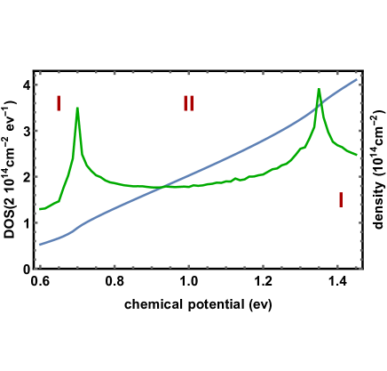
Figure 4: Electron density and DOS as function of the chemical potential $\mu$.of WSM with $\kappa=1.3$. DOS has cusps at both I to II transitions. Between the transitions it is nearly constant in the range of densities from $1.1\times 10^{14}/cm^{2}$ to $4.\times 10^{14}/cm^{2}$.

II.3 Coulomb repulsion

The electron-electron repulsion in the layered WSM can be presented in the form,

$$V=\frac{e^{2}}{2}\sum\nolimits_{\mathbf{n}l\mathbf{n}^{\prime}l^{\prime}}n_{\mathbf{n}l}v_{\mathbf{n-n}^{\prime},l-l^{\prime}}^{C}n_{\mathbf{n}^{\prime}l^{\prime}}=\frac{e^{2}}{2N_{s}^{2}}\sum\nolimits_{\mathbf{q}ll^{\prime}}n_{\mathbf{q}l}n_{-\mathbf{q}l^{\prime}}v_{\mathbf{q,}l-l^{\prime}}^{C}\text{,}$$ (7)

where $v_{\mathbf{n-n}^{\prime},l-l^{\prime}}^{C}$ is the ”bare” Coulomb interaction between electrons with Fourier transform $v_{\mathbf{q},l-l^{\prime}}^{C}=v_{\mathbf{q}}^{2D}e^{-dq\left|l-l^{\prime}\right|}$, $v_{\mathbf{q}}^{2D}=2\pi e^{2}/q\epsilon$. Here $\epsilon$ is the dielectric constant of the intercalator material

The long range Coulomb interaction is effectively taken into account using the RPA approximation.

III Screening in layered WSM.

The screening in the layered system can be conveniently partitioned into the screening within each layer described by the polarization function $\Pi_{\mathbf{q}n}$ and electrostatic coupling to carriers in other layers. We start with the former.

III.1 Polarization function of the electron gas in Layered WSM

In a simple Fermi theory of the electron gas in normal state with Coulomb interaction between the electrons in RPA approximation the Matsubara polarization is calculated as a simple minus ”fish” diagram Elliasson in the form:

$$\Pi_{\mathbf{q}n}=-\left(-2T\text{Tr}\sum\nolimits_{\mathbf{p}m}g_{\mathbf{p}m}g_{\mathbf{p+q},m+n}\right)\text{.}$$ (8)

Using the GF of Eq.(6), one obtain:

$$\Pi_{\mathbf{q}n}=4T\sum\nolimits_{\mathbf{p}m}\frac{\left(i\omega_{m}+A\right)\left(i\omega_{m}+B\right)+C}{\left[\left(i\omega_{m}+A\right)^{2}-\alpha^{2}\right]\left[\left(i\omega_{m}+B\right)^{2}-\beta^{2}\right]}\text{,}$$ (9)

where

$$A = -d_{\mathbf{p}}^{0};B=i\omega_{n}-d_{\mathbf{p+q}}^{0};\text{ \ \ }C=d_{\mathbf{p}}^{x}d_{\mathbf{p+q}}^{x}+d_{\mathbf{p}}^{y}d_{\mathbf{p+q}}^{y};$$ (10)

$$\alpha^{2} = d_{\mathbf{p}}^{x2}+d_{\mathbf{p}}^{y2};\text{ \ \ }\beta^{2}=d_{\mathbf{p+q}}^{x2}+d_{\mathbf{p+q}}^{y2}\text{.}$$

Performing summation over $m$, one obtains:

$$\Pi_{\mathbf{q}n}=-\sum\nolimits_{\mathbf{p}}\left\{\begin{array}[]{c}\frac{\alpha^{2}-\alpha(A-B)+C}{\alpha\left[\left(A-B-\alpha\right)^{2}-\beta^{2}\right]}\tanh\frac{\alpha-A}{2T}+\frac{a^{2}+\alpha(A-B)+C}{\alpha\left[\left(A-B+\alpha\right)^{2}-\beta^{2}\right]}\tanh\frac{\alpha+A}{2T}\\ +\frac{\beta^{2}+\beta\left(A-B\right)+C}{\beta\left[\left(A-B+\beta\right)^{2}-\alpha^{2}\right]}\tanh\frac{\beta-B}{2T}+\frac{\beta^{2}-\beta\left(A-B\right)+C}{\beta\left[\left(A-B-\beta\right)^{2}-\alpha^{2}\right]}\tanh\frac{\beta+B}{2T}\end{array}\right\}\text{.}$$ (11)

Now we turn to screening due to other layers.

III.2 Screening in a layered system

Coulomb repulsion between electrons in different layers $l$ and $l^{\prime}$ within the RPA approximation is determined by the following integral equation:

$$V_{\mathbf{q,}l-l^{\prime}\mathbf{,}n}^{RPA}=v_{\mathbf{q},l-l^{\prime}}^{C}+\Pi_{\mathbf{q}n}\sum\nolimits_{l^{\prime\prime}}v_{\mathbf{q},l-l^{\prime\prime}}^{C}V_{\mathbf{q},l^{\prime\prime}-l^{\prime}\mathbf{,}n}^{RPA}\text{.}$$ (12)

The polarization function $\Pi_{\mathbf{q}n}$ in 2D was calculated in the previous subsection. This set of equations is decoupled by the Fourier transform in the $z$ direction,

$$V_{\mathbf{q,}q_{z},n}^{RPA}=\frac{v_{\mathbf{q},q_{z}}^{C}}{1-\Pi_{\mathbf{q}n}v_{\mathbf{q},q_{z}}^{C}}\text{ , \ }$$ (13)

where

$$v_{\mathbf{q},q_{z}}^{C}=\sum\nolimits_{l}v_{\mathbf{q}}^{2D}e^{iq_{z}l-qd\left|l\right|}=v_{\mathbf{q}}^{2D}\frac{\sinh\left[qd\right]}{\cosh\left[qd\right]-\cos\left[dq_{z}\right]}\text{.}$$ (14)

The screened interaction in a single layer therefore is is given by the inverse Fourier transform Elliasson :

$$V_{\mathbf{q,}l-l^{\prime},n}^{RPA}=\frac{d}{2\pi}\int_{q_{z}=-\pi/d}^{\pi/d}e^{iq_{z}d\left(l-l^{\prime}\right)}\frac{v_{\mathbf{q},q_{z}}^{C}}{1-\Pi_{\mathbf{q}n}v_{\mathbf{q},q_{z}}^{C}}\text{.}$$ (15)

Considering screened Coulomb potential at the same layer $l=l^{\prime},\$the integration gives,

$$V_{\mathbf{q}n}^{RPA}=\frac{v_{\mathbf{q}}^{2D}\sinh\left[qd\right]}{\sqrt{b_{\mathbf{q}n}^{2}-1}}\text{,}$$ (16)

where $b_{\mathbf{q}n}=\cosh\left[dq\right]-v_{\mathbf{q}}^{2D}\Pi_{\mathbf{q}n}\sinh\left[dq\right]$. This formula is reliable only away from plasmon region $b_{\mathbf{q}n}>1$. It turns out that to properly describe superconductivity, one can simplify the calculation at low temperature by considering the static limit $\Pi_{\mathbf{q}n}\simeq\Pi_{\mathbf{q}0}$. Consequently the potential becomes static: $V_{\mathbf{q}}^{RPA}\equiv V_{\mathbf{q},n=0}^{RPA}$.

IV Superconductivity

Superconductivity in WSM is caused by a conventional phonon pairing. The leading mode is an optical phonon mode assumed to be dispersionless. with energy $\Omega$. The effective electron-electron attraction due to the electron - phonon attraction opposed by Coulomb repulsion (pseudo - potential) mechanism creates pairing below $T_{c}$. Further we assume the singlet $s$-channel electron-phonon interaction and neglect the inter-layers electrons pairing.  In order to describe superconductivity, one should ”integrate out” the phonon and the spin fluctuations degrees of freedom to calculate the effective electron - electron interaction. We start with the phonons. The Matsubara action for effective electron-electron interaction via in-plane phonons and direct Coulomb repulsion calculated in the previous Section. It important to note that unlike in metal superconductors where a simplified pseudo - potential approach due to McMillan and other McMillan , in 2D and layered WSM, one have to resort to a more microscopic approach.

IV.1 Effective attraction due to phonon exchange opposed by the effective Coulomb repulsion

The free and the interaction parts of the effective electron action (”integrating phonons”+RPA Coulomb interaction) in the quasi - momentum - Matzubara frequency representation, $S=S^{e}+S^{int}$,

$$S^{int}=\frac{1}{2T}\sum\nolimits_{\mathbf{q}ll^{\prime}mm^{\prime}}n_{\mathbf{q}ln}\left(\delta_{ll^{\prime}}V_{\mathbf{q,}m-m^{\prime}}^{ph}+V_{\mathbf{q},l-l^{\prime}}^{RPA}\right)n_{-\mathbf{q},-l^{\prime},-n^{\prime}}\text{.}$$ (17)

Here $n_{\mathbf{q}ln}=\sum\nolimits_{\mathbf{p}}\psi_{\mathbf{p}ln}^{\ast sI}\psi_{\mathbf{q-p,}l,n}^{sI}$ the Fourier transform of the electron density and $S^{e}$ was defined in Eq.(5). The effective electron - electron coupling due to phonons is:

$$\text{ \ }V_{\mathbf{q}m}^{ph}=-\left(\frac{\sqrt{3}}{2}\right)^{2}\frac{g^{2}\Omega}{\omega_{m}^{b2}+\Omega^{2}}\text{,}$$ (18)

where the bosonic frequencies are $\omega_{m}^{b}=2\pi mT$.

IV.2 Gorkov Green’s functions and the s-wave gap equations

Normal and anomalous (Matsubara) intra - layer Gorkov Green’s functions are defined by expectation value of the fields, $\left\langle\psi_{\mathbf{k}nl}^{Is}\psi_{\mathbf{k}nl}^{\ast s^{\prime}J}\right\rangle=\delta^{ss^{\prime}}G_{\mathbf{k}n}^{IJ}$ and $\left\langle\psi_{\mathbf{k}nl}^{Is}\psi_{-\mathbf{k,-}n,l}^{Js^{\prime}}\right\rangle=\varepsilon^{ss^{\prime}}F_{\mathbf{k}n}^{IJ}$, while the gap function is

$$\Delta_{\mathbf{q}n}^{IJ}=\sum\nolimits_{\mathbf{p}m}V_{\mathbf{q-p,}n-m}F_{\mathbf{p}m}^{IJ},$$ (19)

where $V_{\mathbf{q}n}=V_{\mathbf{q}n}^{ph}+V_{\mathbf{q}n}^{RPA}$ is a sublattice scalar. The gap equations in the sublattice matrix form are derived from Gorkov equations in Appendix B:

$$\Delta_{\mathbf{q}n}=-\sum\nolimits_{\mathbf{p}m}V_{\mathbf{q-p,}n-m}g_{\mathbf{p}m}\left\{I+\Delta_{\mathbf{p}m}g_{-\mathbf{p},-m}^{t}\Delta_{-\mathbf{p},-m}^{\ast}g_{\mathbf{p}m}\right\}^{-1}\Delta_{\mathbf{p}m}g_{-\mathbf{p},-m}^{t}\text{.}$$ (20)

In numerical simulation the gap equation was solved iteratively. Relatively large space cutoff $N_{s}=256$ is required. The frequency cutoff $N_{t}=128$ was required due to low temperatures approached. Typically $15-25$ iterations were required. The parameters used were $\Omega=16meV$. The electron - phonon coupling $g=20meV$. Now we turn to results concentrating on two puzzling experimental results of ref.Zhang22 .

IV.3 Independence of $T_{c}$ on density in topological type II phase

In Fig.5 the critical temperature for various values of density are plotted.

The blue points are for dielectric constantZhang22 , $\varepsilon=16$, describing the intercalated imidazole cations $[C_{2}MIm]$ dc . The inter - layer distance was kept at $d=10.5A$.

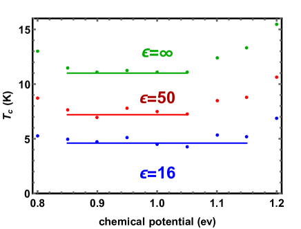
Figure 5: Critical temperature of transition to superconducting state in type II layered WSM is shown as function of chemical potential (can be translated into carrier density via Fig.4). Three values of dielectric constant of the intercalant for fixed interlayer distance are shown. Parameters of the electron gas are the same as in previous figures.

The significance and generatiozation of the observation are discussed below.

IV.4 Increase of $T_{c}$ with  dielectric constant of intercalator materials

The main idea of the paper is that the difference in $T_{c}$ between different intercalators is attributed not to small variations in the inter - layer spacing $d$, but rather to large differences in the dielectric constant of the intercalating materials due to its effect on the screening. In experiment of ref.Zhang22 the imidazole cations $[C_{2}MIm]^{+}$ (1- ethyl - 3 - methyl - imidazolium) are short moleculesdc have $\epsilon=16$, while $[C_{6}MIm]^{+}$ (1- hexy l - 3 - methy l - imidazolium) are long moleculesdc2 with a larger value $\epsilon\simeq 50$. The inter - layer distance $d$ is slightly dependent intercalators changing from $10.5\mathring{A}$ to $11.7\mathring{A}$ . The blue points in Fig 5 describe a material with dielectric constant $\varepsilon=16$ should. This is contrasteddc2 with the $\varepsilon=50$ material, see the red point. Neglecting the Coulomb repulsion, see the green points, critical temperature (a much simpler calculation of $T_{c}$ in this case similar to that in ref.Rosenstein17 is needed in this case) becomes yet higher. This demonstrate the importance of the Coulomb repulsion in a quasi 2D system. Superconductivity is weaker for monolayer on substrate since both air and substrate have smaller dielectric constants and hence weaker screen the Coulomb repulsion.

V Discussion and conclusion

To summarize we have developed a theory of superconductivity in layered type II Weyl semi-metals that properly takes into account the Coulomb repulsion. The generalization goes beyond the simplistic pseudo - potential approach due to McMillanMcMillan and others and depends essentially on the intercalating material. The theory allows to explain the two puzzling phenomena observed recently in layered intercalated $MoTe_{2}$ WSW compound Zhang22

The first experimental observation is that the gate voltage (changes in the chemical potential or equivalently in density) has no impact on critical temperature $T_{c}$. For the 3D density range $8.\times 10^{20}cm^{-3}-3.6\times 10^{21}cm^{-3}$ the temperature changes within $5\%$. For the intercalating material $[C_{2}MIm]^{+}$ with inter - layer distance $d=10.5A$ the 2D density range translates into $8.4\times 10^{13}cm^{-2}-3.8\times 10^{14}cm^{-2}$ wth slightly larger spacings $d=11.7A$ shown in Figs 2-5. This feature is explained purely topologically, see schematic Fig.1. In the type II density range the shape of both pieces of the Fermi surface (the blue - yellow boundaries in Fig1b and Fig1c) largely does not depend on the density (that is proportional to the area of the blue part of the surface) leading, see Fig. 4 to approximate independence of the density of states (DOS) $N\left(0\right)$ of chemical potential $\mu$. This feature is akin to the DOS independence on $\mu$ for a parabolic (topologically type I like in Fig.1a) band in purely 2D materials, but has completely difficult origin.

Using the somewhat naive BCS formula

$$T_{c}\simeq\Omega\text{ }e^{-N\left(0\right)g_{eff}^{2}}\text{.}$$ (21)

Here $\Omega$ is the phonon frequency and $g_{eff}$ the effective electron - phonon coupling. Assuming that both $\Omega$ and $g$ do not depend on the density one arrives at a conclusion that in the type II topological phase the critical temperature is density independent .

The second experimental observationZhang22 was that $T_{c}$ is in fact very sensitive to the intercalating material. For imidazole cations $[C_{2}MIm]^{+}$ the critical temperature is $T_{c}=4.2K$, while for $[C_{6}MIm]^{+}$ the temperature jumps to $T_{c}=6.6K$ or $6.9K$ depending on the intercalation method. The inter - layer distance $d$ is slightly dependent intercaltors increasing from $10.5\mathring{A}$ to $11.7\mathring{A}$ . Our calculation demonstrates that the difference in $T_{c}$ between different intercalators cannot be attributed to small variations in the inter - layer spacing $d$. On the contrary there are large differences in the dielectric constant of the intercalating materials. While $[C_{2}MIm]^{+}$ havedc a relatively small dielectric constant $\epsilon=16$, $[C_{6}MIm]^{+}$ is estimateddc2 in the range $\epsilon=40-60$. Our theory accounts the difference in $T_{c}$ due to changes in the screening of the Coulomb potential due to the inter - layer insulator.

VI
Acknowledgements.

This work was supported by NSC of R.O.C. Grants No. 101-2112-M-009-014-MY3.

VII

VIII Appendix A. Details of the model

The system considered in the paper is fitted for the following values of the hipping and the tilt parameter. The dimensionless tilt parameter was taken from ref.Zhang22 $\kappa=1.3$. The hopping $\gamma=500$ $meV$ and $t=2$. The calculations were performed on the discrete reciprocal lattice $k_{1},k_{2}=1,...N_{s}$ with $N_{s}=256$. Reciprocal lattice basis vectors are,

$$\mathbf{b}_{1}=2\pi\left(1,\frac{1}{\sqrt{3}}\right);\text{ \ \ \ }\mathbf{b}_{2}=2\pi\left(1,-\frac{1}{\sqrt{3}}\right),$$ (22)

so that a convenient representation is $\mathbf{k}=\frac{k_{1}}{N_{s}}\mathbf{b}_{1}+\frac{k_{2}}{N_{s}}\mathbf{b}_{2}$ with

$$k_{x}=\frac{2\pi}{N_{s}}\left(k_{1}+k_{2}\right),\text{ \ \ }k_{y}=\frac{2\pi}{\sqrt{3}N_{s}}\left(k_{1}-k_{2}\right)\text{.}$$ (23)

IX Appendix B. Derivation of the two sublattice gap equation

IX.1 Green’s functions and the s-wave Gorkov equations

We derive the Gorkov’s equations (GE) within the functional integral approachNO starting from the effective electron action for grassmanian fields $\psi^{\ast X},\psi^{Y}$.

$$S=\frac{1}{T}\left\{\psi^{\ast X}\left(G_{0}^{-1}\right)^{XY}\psi^{Y}+\frac{1}{2}\psi^{\ast Y}\psi^{Y}V^{YX}\psi^{\ast X}\psi^{X}\right\},$$ (24)

where $X,Y$ denote space coordinate, sublattices (pseudospin) and spin of the electron. Finite temperature properties of the condensate are described at temperature $T$ by the normal and the anomalous Matsubara Greens functions for spin singlet state.

The GE in functional form are:

$$\left\langle\psi^{A}\psi^{\ast B}\right\rangle\frac{\delta}{\delta\psi^{\ast C}}\left\langle\frac{\delta S}{\delta\psi^{\ast B}}\right\rangle+\left\langle\psi^{A}\psi^{B}\right\rangle\frac{\delta}{\delta\psi^{\ast C}}\left\langle\frac{\delta S}{\delta\psi^{B}}\right\rangle=0;$$ (25)

$$\left\langle\psi^{A}\psi^{\ast B}\right\rangle\frac{\delta}{\delta\psi^{C}}\left\langle\frac{\delta S}{\delta\psi^{\ast B}}\right\rangle+\left\langle\psi^{A}\psi^{B}\right\rangle\frac{\delta}{\delta\psi^{C}}\left\langle\frac{\delta S}{\delta\psi^{B}}\right\rangle=\delta^{AC}\text{.}$$ (26)

Performing the calculations and using the normal and anomalous Green functions in the form $F^{AB}=\left\langle\psi^{A}\psi^{B}\right\rangle;G^{AB}=\left\langle\psi^{A}\psi^{\ast B}\right\rangle,$

one obtains:

$$F^{AX}\left\{\left(G_{0}^{-1}\right)^{CX}-v^{XC}G^{CX}+v^{CX}G^{XX}\right\}+G^{AX}v^{XC}F^{XC}=0.$$ (27)

Skipping second and third terms in bracket in this expression and defining, superconducting gap $\Delta^{AB}=v^{AB}F^{AB}$, one rewrites as a matrix products:

$$\left(G_{0}^{-1}\right)^{CX}F^{XA}=G^{AX}\Delta^{XC}\text{.}$$ (28)

The first GE (multiplied from left by $G_{0}$) is,

$$F^{AB}=-G^{AX}G_{0}^{BY}\Delta^{XY}\text{,}$$ (29)

while the second GE similarly is:

$$G^{AB}-G^{AX}\Delta^{XY}G_{0}^{ZY}\Delta^{\ast ZU}G_{0}^{UB}=G_{0}^{AB}\text{.}$$ (30)

IX.2 Frequency-quasi-momentum and the spin-sublattice decomposition

The generalized index $A$ contains the space variables (space + Matsubara time, $a$), spin $s$ and the sublattice $I$. After performing the Fourier series with combined quasi - momentum - frequency $\alpha$:

$$F_{ab}^{s_{1}s_{2}IJ} = \epsilon^{s_{1}s_{2}}\sum\nolimits_{\alpha}e^{i\alpha\left(a-b\right)}F_{\alpha}^{IJ};\text{ \ }\Delta_{ab}^{s_{1}s_{2}IJ}=\epsilon^{s_{1}s_{2}}\sum\nolimits_{\alpha}e^{i\alpha\left(a-b\right)}\Delta_{\alpha}^{IJ};$$ (31)

$$G_{0ab}^{s_{1}s_{2}IJ} = \delta^{s_{1}s_{2}}\sum\nolimits_{\alpha}e^{i\alpha\left(a-b\right)}g_{\alpha}^{IJ};\text{ \ }V_{ab}^{s_{1}s_{2}IJ}=\sum\nolimits_{\alpha}e^{i\alpha\left(a-b\right)}v_{\alpha}\text{.}$$

Substituting spins into Eq.(29,30), one obtains in the sublattice matrix form

$$F_{\alpha} = -G_{\alpha}\Delta_{\alpha}g_{-\alpha}^{t};$$ (32)

$$G_{\alpha} = G_{0\alpha}\left\{I+\Delta_{\alpha}g_{-\alpha}^{t}\Delta_{-\alpha}^{\ast}G_{0\alpha}\right\}^{-1}\text{,}$$

Convoluting the first GE by $v_{\nu}$ one obtains:

$$\Delta_{\omega}=-\sum\nolimits_{\nu}v_{\omega-\nu}G_{\nu}\Delta_{\nu}g_{-\nu}^{t}\text{.}$$ (33)

The solution of the second GE for $G$ is:

$$G_{\alpha}=g_{\alpha}\left\{I+\Delta_{\alpha}g_{-\alpha}^{t}\Delta_{-\alpha}^{\ast}g_{\alpha}\right\}^{-1}\text{.}$$ (34)

Substituting into the first GE one obtain Eq.(20) in the text.

References

(1) Katsnelson M.I. 2012 The Physics of
Graphene, (Cambridge, Cambridge University Press).
(2) Soluyanov A. A. , Gresch D. ,Wang Z. ,Wu Q. ,Troyer M.
,Dai X. & Bernevig B. A. 2015, Nature527, 495.
(3) Yu Z.-M. , Yao Y. , and Yang S. A. 2016 Phys. Rev.
Lett. 117, 077202.
(4) O’Brien T. E. ,Diez M. , and Beenakker C. W. J. , 2016
Phys.Rev. Lett.116, 236401.
(5) Wang C. et al. 2018 Nature, 555, 231; Lin,
Z. et al. 2018 Nature, 562, 254; Huang H.,Zhou S. and
DuanW., 2016 Phys.Rev.B94 121117; Yan M. et al, Nature Comm. 2017 8, 257; Furue Y. 2021 et al Phys. Rev. B104,144510.
(6) Zhang H. , Rousuli A. ,Zhang K. ,Zhong H. ,Wu Y. ,Yu P.
,Zhou S. 2022 2D Materials 9 045027.
(7) Das Sarma S. andLi Q. 2013 Phys. Rev. B88, 081404(R);Brydon P.M.R. ,Das Sarma S. ,Hui H.-Y. and Sau J. D. 2014
Phys. Rev. B90, 184512;Li D. ,Rosenstein B. ,Shapiro B.
Ya. , andShapiro I. 2014 Phys. Rev. B 90 054517.
(8) Fu L. and Berg E. 2010 Phys. Rev. Lett.105, 097001.
(9) Zhang J.-L. et al. 2012 Front. Phys., 7, 193.
(10) Alidoust M. , Halterman K. , and Zyuzin A. A. 2017 Phys. Rev. B95, 155124.
(11) Li D. , Rosenstein B. , Shapiro B. Ya. , and Shapiro
I. 2017 Phys. Rev. B95, 094513.
(12) Shapiro B Ya , Shapiro I , Li D. and Rosenstein B.
2018 J. Phys.:Condens. Matter30 335403.
(13) Wang S. T. et al. 2012 Appl. Phys. Let. 101, 183110.
(14) Hawrylak P. , Eliasson G. , and Quinn J. J., 1988
Phys. Rev. B37 10187.
(15) Bilbro G. and McMillan L. 1976 Phys. Rev. B14 1887.
(16) Katayama S. ,Kobayashi A. ,Suzumura Y. 2006 J.
Phys. Soc. Japan75, 054705;Goerbig M. O. , Fuchs J.
-N.,Montambaux G. , Piéchon F. 2008 Phys. Rev. B78,
045415; Hirata M. et al. 2016 Nature Commun.7 12666.
(17) Beal A R and Hughes H P 1979 J. Phys. C: Solid State Phys.
12 881 .
(18) Yang L., Fishbine B. H. , Migliori A. and Pratt L.R., 2010 J.
Chem. Phys. 132 044701.
(19) Negele J.W. and Orlando H. , Quantum Many Particle
Systems, 1998 Aspen, Advanced Book Classics, Westview Press.