Wigner Gaussian dynamics: simulating the anharmonic and quantum ionic motion

Abstract

The atomic motion controls important properties of materials, such as thermal transport, phase transitions, and vibrational spectra. However, simulating the ionic dynamics is exceptionally challenging when quantum fluctuations are relevant (e.g., at low temperatures or with light atoms) and the energy landscape is anharmonic. In this work, we present the Time-Dependent Self-Consistent Harmonic Approximation (TDSCHA) [L. Monacelli and F. Mauri, Phys. Rev. B 103, 104305 (2021)] in the Wigner framework, paving the way for the efficient computation of the nuclear motion in systems with sizable quantum and thermal anharmonic fluctuations. Besides the improved numerical efficiency, the Wigner formalism unveils the classical limit of TDSCHA and provides a link with the many-body perturbation theory of Feynman diagrams.

We further extend the method to account for the non-linear couplings between phonons and photons, responsible, e.g., for a nonvanishing Raman signal in high-symmetry Raman inactive crystals, firstly discussed by Rasetti and Fermi. We benchmark the method in phase III of high-pressure hydrogen ab initio. The nonlinear photon-phonon coupling reshapes the IR spectra and explains the high-frequency shoulder of the H2 vibron observed in experiments.

The Wigner TDSCHA is computationally cheap and derived from first principles. It is unbiased by assumptions on the phonon-phonon and phonon-photon scattering and does not depend on empirical parameters. Therefore, the method can be adopted in unsupervised high-throughput calculations.

I Introduction

The burst of computational resources accomplished during the last decades unlocked the path to material design: we can synthesize in silico new materials and measure their properties before the experimental realization. High-throughput simulations are driving the discovery of new cathode materials for batteries [1], superconductor hydrides [2], and 2D materials [3], among others. However, the available toolchain for high-throughput simulation fails when anharmonicity is strong. In these cases, the harmonic approximation and perturbative approaches are inadequate. This happens in hydrides where quantum fluctuations alter the free energy landscape [4, 5], phase diagram of hydrogen-rich compounds like high-pressure ice [6, 7] and solid hydrogen [8, 9], and materials undergoing displacive phase transition like charge density wave (CDW) transition metal dichalcogenides [10, 11, 12, 13].

Lattice anharmonicity influences the vibrational spectra, the optical properties, and the conductivity of a crystal [14]. These consist in the main experimental signatures of the atomic structure and phase transitions when diffraction is not possible due to small sample size or low cross-section. Examples include solid hydrogen [15, 16], high-pressure water [17], and hydrides superconductors [18].

Furthermore, accurate simulations of the ionic motion are fundamental in quantum paraelectric perovskites like KTaO3 [19] and SrTiO3 [20], in which the ferroelectric phase transition is hindered by quantum ionic fluctuations. These materials play a crucial role in applications of nonlinear phononics [21, 22], where the anharmonic coupling between phonons induces transient structural changes and crystal-symmetry breaking upon light pumping [22, 23]. Their theoretical and computational investigation has been limited to models assuming specific patterns of phonon-phonon and phonon-photon interactions [24, 21]. Moreover, the lack of an unsupervised technique prevents the systematic and high-throughput search for better materials in nonlinear phononics.

The Time-Dependent Self-consistent Harmonic Approximation (TDSCHA) [25, 26] provides an efficient numerical solution for finite-temperature nuclear dynamics with quantum and anharmonic fluctuations beyond perturbative approaches. This method has been successfully applied to simulate Raman and IR spectra of high-pressure molecular hydrogen [15] and to characterize the quantum paraelectric transition in KTaO3 [19].

TDSCHA approximates the nuclear density matrix with the most general Gaussian. This leads to a more efficient technique than path-integral (PI) methods, where classical-like trajectories of different replicas are sampled [27, 28, 29, 30]. Instead, it shares some similarities with the Linearized Semi-Classical Initial Value Representation method (LSC-IVR) [31], in which an approximate quantum initial condition for the ionic system [32, 33, PoulsenWignerdistrSamplin, 34] is evolved subject to classical dynamics. Among all these methods, TDSCHA is the computationally most efficient for medium-sized systems (containing hundreds of ions).

However, the exceptional complexity of the original TDSCHA formulation hampers its physical interpretations, and many questions remain unanswered. For example, how does it relate to other approaches employed in quantum chemistry [31]? Which phonon scattering mechanisms is the theory able to describe? What are the limitations of its applicability? And how does the theory behave in the classical limit?

In this work, we reformulate the TDSCHA in the Wigner formalism, where the density matrix is expressed as a function of position and momentum in a quantum-phase space [35] (Sec. II). In this way, the TDSCHA equations are simplified, and the nuclear evolution is governed only by the position-momentum averages and correlators at a fixed time (Sec. III). The $\hbar$ vanishes from the propagator, thus, the initial condition determines whether the evolution is quantum or classical, and they share the same computational cost.

The TDSCHA linear response in the Wigner formalism (Sec. IV) becomes very intuitive and compact. The propagator is reformulated in terms of Feynman diagrams, establishing a simple connection with other many-body approaches like the Self-Consistent Phonon (SCP) technique [36, 37]. In Sec. V, we extend the formalism to allow for the simulation of nonlinear coupling between phonons and photons. Finally, we benchmark the theory on the IR spectrum of high-pressure hydrogen phase III (Sec. VI), where it is demonstrated that the high-frequency overtone observed in [38] is a result of the aforementioned nonlinear coupling between photons and phonons.

We start by reviewing the classical and quantum dynamics within the Wigner formalism in the next Section (II).

II Nuclear dynamics

Here, we review the Wigner formalism for the exact nuclear evolution and compare the quantum and classical dynamics of $N$ ions in a closed system. Nuclear spins and ionic exchange are neglected.

II.1 Classical nuclear evolution

In the classical limit, the nuclei behave like dimensionless particles that move according to the time-dependent Hamiltonian

$$H(t)=\sum_{a=1}^{3N}\frac{P^{2}_{a}}{2m_{a}}+V^{(\text{tot})}(\bm{R},t).$$ (1)

For brevity, we indicate with $a=(i,\alpha)$ a composite index with the atomic index $i$ and Cartesian index $\alpha$, $m_{a}=m_{i}$ is the mass of atom $i$, $\small P_{a}=P_{i,\alpha}$ is the momentum of atom $i$ along the $\alpha$ direction and $\small\bm{R}=\left(\bm{R}_{1},..,\bm{R}_{N}\right)$ represents a configuration of atomic positions. The total potential can be divided into an internal static interaction and an external time-dependent perturbation

$$V^{(\text{tot})}(\bm{R},t)=V^{(\text{BO})}(\bm{R})+V^{(\text{ext})}(\bm{R},t),$$ (2)

where $\small V^{(\text{BO})}(\bm{R})$ is the nuclear interaction mediated by the electrons within the Born-Oppenheimer approximation, i.e. the ground state electronic energy at fixed nuclear configurations. It can be evaluated as the total energy of an ab-initio calculation like density-functional theory (DFT), or an appropriately parametrized force field. $\small{V^{(\text{ext})}(\bm{R},t)}$ is the external time-dependent potential. It encodes the interaction between the probe (usually an electromagnetic field) and the ions, mediated by the electrons.

Physical properties are computed as averages over the phase-space of the corresponding observable with the time-dependent probability distribution (normalized and positive-definite) $\rho_{\text{cl}}(\bm{R},\bm{P},t)$:

$$\left\langle O\right\rangle_{\rho_{\text{cl}}}=\int d\bm{R}\int d\bm{P}O(\bm{R},\bm{P})\rho_{\text{cl}}(\bm{R},\bm{P},t).$$ (3)

In a closed system, $\rho_{\text{cl}}(\bm{R},\bm{P},t)$ evolves according to the Liouville equation

$$\frac{\partial}{\partial t}\rho_{\text{cl}}(\bm{R},\bm{P},t)+i\mathcal{L}^{\text{cl}}\rho_{\text{cl}}(\bm{R},\bm{P},t)=0.$$ (4)

The classical Liouville operator is defined as

$$i\mathcal{L}^{\text{cl}}\circ=-H(t)\overset{\leftrightarrow}{\Lambda}\circ$$ (5)

and $\overset{\leftrightarrow}{\Lambda}$ is the Poisson brackets operator.

$$\overset{\leftrightarrow}{\Lambda}=\sum_{a=1}^{3N}\left(\overset{\leftarrow}{\partialderivative{R_{a}}}\overset{\rightarrow}{\partialderivative{P_{a}}}-\overset{\leftarrow}{\partialderivative{P_{a}}}\overset{\rightarrow}{\partialderivative{R_{a}}}\right),$$ (6)

where the arrows indicate on which side the derivative is applied:

$$A\overset{\leftrightarrow}{\Lambda}B=\{A,B\}=\sum_{a=1}^{3N}\left(\partialderivative{A}{R_{a}}\partialderivative{B}{P_{a}}-\partialderivative{A}{P_{a}}\partialderivative{B}{R_{a}}\right).$$ (7)

Eq. (4) preserves the phase-space volume, which behaves as an incompressible fluid, so probability can not be created nor destroyed leading to entropy conservation.

II.2 Quantum nuclear evolution

The Wigner formalism describes the quantum nuclear evolution in terms of position and momentum degrees of freedom, in a way analogous to the classical Liouville propagation discussed in Sec. II.1. Thus, the differences between quantum and classical dynamics are clear.

The Wigner quasi-distribution [39], defined as a Fourier transform of the Von Neumann density operator $\hat{\rho}(t)$, is the quantum analogue of the classical probability distribution in the phase space. It is given by

$$\rho_{\text{w}}(\bm{R},\bm{P},t)=\int\frac{d\bm{R}^{\prime}e^{-\frac{i}{\hbar}\bm{P}\cdot\bm{R}^{\prime}}}{(2\pi\hbar)^{3N}}\bra{\bm{R}+\frac{\bm{R}^{\prime}}{2}}\hat{\rho}(t)\ket{\bm{R}-\frac{\bm{R}^{\prime}}{2}}.$$ (8)

We remark that Eq. (8) is normalized, as in the classical case, but, in general, it is not positive-definite [40], hence it can not be interpreted as a probability distribution. Still, it encodes all the information on the system.

Similarly, the Wigner expression for an operator $\hat{O}$ is defined as

$$\small O_{\text{w}}(\bm{R},\bm{P})=\int d\bm{R}^{\prime}e^{-\frac{i}{\hbar}\bm{P}\cdot\bm{R}^{\prime}}\bra{\bm{R}+\frac{\bm{R}^{\prime}}{2}}\hat{O}\ket{\bm{R}-\frac{\bm{R}^{\prime}}{2}},$$ (9)

so that quantum averages in the Wigner formalism have the same expression as the classical ones (Eq. (3)):

$$\left\langle O_{\text{w}}\right\rangle_{\rho_{\text{w}}}=\int d\bm{R}\int d\bm{P}O_{\text{w}}(\bm{R},\bm{P})\rho_{\text{w}}(\bm{R},\bm{P},t).$$ (10)

The Wigner-Liouville equation controls the time evolution of $\rho_{\text{w}}(\bm{R},\bm{P},t)$

$$\frac{\partial}{\partial t}\rho_{\text{w}}(\bm{R},\bm{P},t)+i\mathcal{L}\rho_{\text{w}}(\bm{R},\bm{P},t)=0,$$ (11)

where $i\mathcal{L}$ is unitary and contains a classical (cl) and a quantum (q) propagator:

$$i\mathcal{L}=i\mathcal{L}^{\text{cl}}+i\mathcal{L}^{\text{q}}.$$ (12)

The classical propagator $i\mathcal{L}^{\text{cl}}$ coincides with Eq. (5). On the other hand, the quantum part depends explicitly on $\hbar$:

$$\small i\mathcal{L}^{\text{q}}\circ=-\sum_{n=1}^{+\infty}\frac{(-\hbar^{2})^{n}}{2^{2n}(2n+1)!}H(t)\left(\overset{\leftrightarrow}{\Lambda}\right)^{2n+1}\circ.$$ (13)

Eq. (13) gives quantum corrections to the dynamics as odd powers of the Poisson brackets operator.

Interestingly, any quadratic potential has $i\mathcal{L}^{\text{q}}=0$, even when its coefficients are time-dependent, e.g.

$$\small H(t)=\sum_{a=1}^{3N}\frac{P^{2}_{a}}{2m_{a}}+\frac{1}{2}\sum_{ab=1}^{3N}(R-R_{0}(t))_{a}K_{0}(t)_{ab}(R-R_{0}(t))_{b}.$$ (14)

The density matrix propagates only according to $i\mathcal{L}^{\text{cl}}$, and the dynamic is independent on $\hbar$. The quantum/classical nature of the system is encoded only in the initial condition.

In the next Section, we will show that TDSCHA [25] shares the same feature since it is based on a Hamiltonian with the same form of Eq. (14), where $\bm{K}_{0}(t)$ and $\bm{R}_{0}(t)$ are evaluated self-consistently from the distribution.

III Gaussian dynamics in the Wigner framework

The TDSCHA constrains the quantum density matrix as the most general time-dependent Gaussian [25]. Since the Wigner transformation is equivalent to a Fourier transform, also the nuclear time-dependent Wigner quasi-distribution is a Gaussian

(15)

where $\mathcal{N}(t)$ is the normalization, defined such that

$$\int d\bm{R}\int d\bm{P}\widetilde{\rho}(\bm{R},\bm{P},t)=1.$$ (16)

$\bm{\mathcal{R}}(t)$, $\bm{\mathcal{P}}(t)$, $\bm{\alpha}(t)$, $\bm{\beta}(t)$, $\bm{\gamma}(t)$ are the time-dependent free parameters of the distribution. In contrast to the general Wigner distribution, Eq. (15) is positive-definite and can be interpreted as the quantum probability distribution. Thanks to the Wigner transformation, it is evident that $\widetilde{\rho}(\bm{R},\bm{P},t)$ is the multidimensional generalization of the one reported in [41] for the 1D case. The position and momentum centroids $\bm{\mathcal{R}}(t)$ and $\bm{\mathcal{P}}(t)$ are $3N$ real vectors and represent, respectively, the instantaneous average position and momentum of the ions:

$$\vspace{-0.25cm}\bm{\mathcal{R}}(t)=\left\langle\bm{R}\right\rangle_{\widetilde{\rho}(t)},\qquad\bm{\mathcal{P}}(t)=\left\langle\bm{P}\right\rangle_{\widetilde{\rho}(t)}.$$ (17)

$\bm{\alpha}(t)$, $\bm{\beta}(t)$ and $\bm{\gamma}(t)$ are $3N\times 3N$ real tensors ($\bm{\alpha}(t)$ and $\bm{\beta}(t)$ are symmetric) and represent the instantaneous position-momentum correlators:

$$\left\langle\delta\widetilde{\bm{R}}(t)\delta\widetilde{\bm{R}}(t)\right\rangle_{\widetilde{\rho}(t)}= \left(\widetilde{\bm{\alpha}}(t)-\widetilde{\bm{\gamma}}(t)\cdot\widetilde{\bm{\beta}}^{-1}(t)\cdot\widetilde{\bm{\gamma}}^{T}(t)\right)^{-1},$$ (18a)

$$\left\langle\delta\widetilde{\bm{R}}(t)\delta\widetilde{\bm{P}}(t)\right\rangle_{\widetilde{\rho}(t)}= -\left(\widetilde{\bm{\gamma}}^{T}(t)-\widetilde{\bm{\beta}}(t)\cdot\widetilde{\bm{\gamma}}^{-1}(t)\cdot\widetilde{\bm{\alpha}}(t)\right)^{-1},$$ (18b)

$$\left\langle\delta\widetilde{\bm{P}}(t)\delta\widetilde{\bm{P}}(t)\right\rangle_{\widetilde{\rho}(t)}= \left(\widetilde{\bm{\beta}}(t)-\widetilde{\bm{\gamma}}^{T}(t)\cdot\widetilde{\bm{\alpha}}^{-1}(t)\cdot\widetilde{\bm{\gamma}}(t)\right)^{-1},$$ (18c)

where $\delta\widetilde{\bm{R}}(t)=\widetilde{\bm{R}}-\widetilde{\bm{\mathcal{R}}}(t)$, $\delta\widetilde{\bm{P}}(t)=\widetilde{\bm{P}}-\widetilde{\bm{\mathcal{P}}}(t)$ and the $\widetilde{\circ}$ indicates a mass-rescaled variable like

$$\widetilde{R}_{a}=\sqrt{m_{a}}R_{a},\qquad\widetilde{P}_{a}=\frac{P_{a}}{\sqrt{m_{a}}}.$$ (19)

The detailed derivation of Eq. (18) is reported in Appendix A.

The dynamics of the Wigner distribution can be obtained by transforming the time-dependent equation of the TDSCHA in the Wigner basis. We prove in Appendix B that this is equivalent to evolve Eq. (15) with a self-consistent Wigner-Liouville equation

$$\vspace{-0.25cm}\frac{\partial}{\partial t}\widetilde{\rho}(\bm{R},\bm{P},t)+i\mathcal{L}^{\text{sc}}\widetilde{\rho}(\bm{R},\bm{P},t)=0,$$ (20)

where

$$i\mathcal{L}^{\text{sc}}\circ=-\mathcal{H}(\widetilde{\rho})\overset{\leftrightarrow}{\Lambda}\circ,$$ (21)

and $\mathcal{H}(\widetilde{\rho})$ is a quadratic time-dependent Hamiltonian that depends self-consistently on $\widetilde{\rho}(t)$:

$$\mathcal{H}(\widetilde{\rho})= \sum_{a=1}^{3N}\frac{P^{2}_{a}}{2m_{a}}+\sum_{a=1}^{3N}\delta R(t)_{a}\left\langle\frac{\partial V^{(\text{tot})}(\bm{R},t)}{\partial R_{a}}\right\rangle_{\widetilde{\rho}(t)}$$ (22)

$$+\frac{1}{2}\sum_{ab=1}^{3N}\delta R(t)_{a}\left\langle\frac{\partial^{2}V^{(\text{tot})}(\bm{R},t)}{\partial R_{a}\partial R_{b}}\right\rangle_{\widetilde{\rho}(t)}\delta R(t)_{b}.$$

Inserting the Wigner-TDSCHA distribution, Eq. (15), in Eq. (20) and substituting the expression of the propagators of Eq. (18) (details in Appendix A), we get the equations of motion

$$\frac{d}{dt}\left\langle\widetilde{\bm{R}}\right\rangle_{\widetilde{\rho}(t)}= \left\langle\widetilde{\bm{P}}\right\rangle_{\widetilde{\rho}(t)},$$ (23a)

$$\frac{d}{dt}\left\langle\widetilde{\bm{P}}\right\rangle_{\widetilde{\rho}(t)}= -\left\langle\frac{\partial V^{(\text{tot})}}{\partial\widetilde{\bm{R}}}\right\rangle_{\widetilde{\rho}(t)},$$ (23b)

$$\frac{d}{dt}\left\langle\delta\widetilde{\bm{R}}\delta\widetilde{\bm{R}}\right\rangle_{\widetilde{\rho}(t)}= \left\langle\delta\widetilde{\bm{R}}\delta\widetilde{\bm{P}}\right\rangle_{\widetilde{\rho}(t)}+\left\langle\delta\widetilde{\bm{P}}\delta\widetilde{\bm{R}}\right\rangle_{\widetilde{\rho}(t)},$$ (23c)

$$\frac{d}{dt}\left\langle\delta\widetilde{\bm{P}}\delta\widetilde{\bm{P}}\right\rangle_{\widetilde{\rho}(t)}= -\left\langle\frac{\partial^{2}V^{(\text{tot})}}{\partial\widetilde{\bm{R}}\partial\widetilde{\bm{R}}}\right\rangle_{\widetilde{\rho}(t)}\cdot\left\langle\delta\widetilde{\bm{R}}\delta\widetilde{\bm{P}}\right\rangle_{\widetilde{\rho}(t)}$$ (23d)

$$-\left\langle\delta\widetilde{\bm{P}}\delta\widetilde{\bm{R}}\right\rangle_{\widetilde{\rho}(t)}\cdot\left\langle\frac{\partial^{2}V^{(\text{tot})}}{\partial\widetilde{\bm{R}}\partial\widetilde{\bm{R}}}\right\rangle_{\widetilde{\rho}(t)},$$

$$\frac{d}{dt}\left\langle\delta\widetilde{\bm{R}}\delta\widetilde{\bm{P}}\right\rangle_{\widetilde{\rho}(t)}= \left\langle\delta\widetilde{\bm{P}}\delta\widetilde{\bm{P}}\right\rangle_{\widetilde{\rho}(t)}$$ (23e)

$$-\left\langle\delta\widetilde{\bm{R}}\delta\widetilde{\bm{R}}\right\rangle_{\widetilde{\rho}(t)}\cdot\left\langle\frac{\partial^{2}V^{(\text{tot})}}{\partial\widetilde{\bm{R}}\partial\widetilde{\bm{R}}}\right\rangle_{\widetilde{\rho}(t)},$$

where to compact the notation we drop the explicit time and position dependence.

The TDSCHA dynamics of Eq. (23) are simpler than the original derivation using the standard formalism of operators in quantum mechanics. As anticipated in Sec. II.2, Eqs (23) do not contain $\hbar$, and the dynamic is the same for quantum and classical distribution. Nevertheless, quantum features are included in the initial condition and preserved during the dynamics. The classical limit of the TDSCHA dynamics was not evident in [25], as the off-diagonal parameters of the density matrix are ill-defined as $\hbar\rightarrow 0$.

This approach is exact in the case of a time-dependent harmonic oscillator since the Wigner distribution is a Gaussian. Thanks to self-consistency, this theory goes beyond harmonic/perturbative methods. No approximations are made on the total potential itself so anharmonic effects are included in a non-perturbative way. The dynamics of Eq. (23) satisfy the conservation of energy and entropy, as expected from a closed system (see Appendix C).

III.1 Equilibrium SCHA in the Wigner formalism

A particular solution of Eq. (23) is the steady state equilibrium in absence of a time-dependent perturbation. From Eqs (23) we get

$$\left\langle\partialderivative{V^{\text{BO}}}{\widetilde{\bm{R}}}\right\rangle_{(0)}= \bm{0}$$ (24a)

$$\left\langle\widetilde{\bm{P}}\right\rangle_{(0)}= \bm{0}\qquad\left\langle\delta\widetilde{\bm{R}}\delta\widetilde{\bm{P}}\right\rangle_{(0)}=\bm{0},$$ (24b)

$$\left\langle\delta\widetilde{\bm{P}}\delta\widetilde{\bm{P}}\right\rangle_{(0)}= \left\langle\delta\widetilde{\bm{R}}\delta\widetilde{\bm{R}}\right\rangle_{(0)}\cdot\left\langle\frac{\partial^{2}V^{(\text{BO})}}{\partial\widetilde{\bm{R}}\partial\widetilde{\bm{R}}}\right\rangle_{(0)},$$ (24c)

where $(0)$ indicates that the averages are performed on $\widetilde{\rho}^{(0)}$, the equilibrium Wigner distribution that solve self-consistently Eq. (24c). Since the average momentum is zero (Eq. 24b), we take $\delta{\bm{P}}=\bm{P}$. As the mixed position-momentum correlation vanishes at equilibrium, the Wigner distribution becomes

$$\widetilde{\rho}^{(0)}(\bm{R},\bm{P})= \mathcal{N}^{(0)}\exp[-\frac{1}{2}\widetilde{\bm{P}}\cdot\left\langle\widetilde{\bm{P}}\widetilde{\bm{P}}\right\rangle_{(0)}^{-1}\cdot\widetilde{\bm{P}}$$ (25)

$$-\frac{1}{2}\delta\widetilde{\bm{R}}\cdot\left\langle\delta\widetilde{\bm{R}}\delta\widetilde{\bm{R}}\right\rangle_{(0)}^{-1}\cdot\delta\widetilde{\bm{R}}\biggl{]}$$

where $\left\langle\widetilde{\bm{P}}\widetilde{\bm{P}}\right\rangle_{(0)}$ and $\left\langle\delta\widetilde{\bm{R}}\delta\widetilde{\bm{R}}\right\rangle_{(0)}$ solve Eq. (24c). Eq. (25) is a steady-state solution of the Wigner TDSCHA equations. Among all distributions, the equilibrium one satisfy

$$\left\langle\delta\widetilde{R}_{a}\delta\widetilde{R}_{b}\right\rangle_{(0)}= \sum_{\mu=1}^{3N}\frac{\hbar(1+2n_{\mu})}{2\omega_{\mu}}e^{a}_{\mu}e^{b}_{\mu},$$ (26a)

$$\left\langle\widetilde{P}_{a}\widetilde{P}_{b}\right\rangle_{(0)}= \sum_{\mu=1}^{3N}\frac{\hbar\omega_{\mu}(1+2n_{\mu})}{2}e^{a}_{\mu}e^{b}_{\mu},$$ (26b)

where $\{\omega_{\mu}\}$ and $\{\bm{e}_{\mu}\}$ define non-interacting phonons of a generalized dynamical matrix

$$\overset{(2)}{D}_{ab}=\left\langle\frac{\partial^{2}V^{(\text{BO})}}{\partial\widetilde{R}_{a}\partial\widetilde{R}_{b}}\right\rangle_{(0)}=\sum_{\mu=1}^{3N}\omega^{2}_{\mu}e^{a}_{\mu}e^{b}_{\mu},$$ (27)

and $n_{\mu}$ is the Bose-Einstein distribution

$$n_{\mu}=\frac{1}{e^{\beta\hbar\omega_{\mu}}-1}.$$ (28)

The equilibrium solution is the one with the minimum free energy at fixed temperature, and in Appendix B we show that it coincides with the Wigner transform of the Self-Consistent Harmonic Approximation (SCHA) density matrix [42, 43, 44]. Our initial condition is constrained to be a Gaussian so we do not have to employ a sampling of the Wigner quasi-distribution [33, 32] as done in Linearized Semi-Classical Initial Value Representation methods (LSC-IVR) [45]. These approaches compute time correlation functions approximating the quantum dynamics with a classical evolution (setting $i\mathcal{L}^{\text{q}}=0$ in Eq. (12)) [31], whereas the TDSCHA evolution is justified from the quantum action principle [25].

III.1.1 Diagrammatic representation of the SCHA

We present a diagrammatic expansion of the SCHA in a quartic potential to clarify the anharmonic processes involved in the theory, and to highlight the differences between SCHA, TDSCHA, and other approaches such as Self-Consistent Phonon (SCP) [36, 37] and perturbation theory.

We define the SCHA propagator through Eq. (27).

$$\bm{\mathcal{G}}^{(0)}(\omega)^{-1}=\omega^{2}-\overset{(2)}{\bm{D}}\overset{\omega=0}{\longrightarrow}-\overset{(2)}{\bm{D}}.$$ (29)

Since the SCHA is a static theory and it is defined through $\omega=0$ quantities. Similarly, one can define the harmonic propagator as

$$\small\bm{g}^{(0)}(\omega)^{-1}=\omega^{2}-\frac{\partial^{2}V^{\text{(BO)}}}{\partial\widetilde{\bm{R}}\partial\widetilde{\bm{R}}}\biggl{|}_{\bm{R}=\bm{\mathcal{R}}_{\text{BO}}}\overset{\omega=0}{\longrightarrow}-\frac{\partial^{2}V^{\text{(BO)}}}{\partial\widetilde{\bm{R}}\partial\widetilde{\bm{R}}}\biggl{|}_{\bm{R}=\bm{\mathcal{R}}_{\text{BO}}},$$ (30)

where $\bm{\mathcal{R}}_{\text{BO}}$ is the minimum of $V^{\text{(BO)}}(\bm{R})$

$$\frac{\partial V^{\text{(BO)}}}{\partial\widetilde{\bm{R}}}\biggl{|}_{\bm{R}=\bm{\mathcal{R}}_{\text{BO}}}=\bm{0},$$ (31)

and the harmonic phonons are the eigenvalues of the second-order expansion of the BO potential around its minimum $\bm{\mathcal{R}}_{\text{BO}}$

$$\frac{\partial^{2}V^{\text{(BO)}}}{\partial\widetilde{R}_{a}\partial\widetilde{R}_{b}}\biggl{|}_{\bm{R}=\bm{\mathcal{R}}_{\text{BO}}}=\sum_{\mu=1}^{3N}\Omega^{2}_{\mu}\epsilon^{a}_{\mu}\epsilon^{b}_{\nu}.$$ (32)

In what follows we use $\bm{g}^{(0)}$ and $\bm{\mathcal{G}}^{(0)}$ to denote the static limit ($\omega=0$) of the propagators introduced in Eqs. (29), (30).

To connect the SCHA with perturbation theory, we expand the BO energy landscape $V^{\text{(BO)}}(\bm{R})$ in a Taylor series around the positions $\bm{\mathcal{R}}_{\text{BO}}$. All the SCHA equations contain averages of all BO potential derivatives

$$\left\langle\frac{\partial^{k}V^{(\text{BO})}}{\partial\widetilde{R}_{b_{1}}..\partial\widetilde{R}_{b_{k}}}\right\rangle_{(0)} =\sum_{n=0}^{\infty}\frac{1}{n!}\sum_{a_{1}..a_{n}=1}^{3N}\overset{(k+n)}{d}_{b_{1}..b_{k}a_{1}..a_{n}}$$ (33)

$$\left\langle\left(\delta\widetilde{R}+\widetilde{\delta}\right)_{a_{1}}..\left(\delta\widetilde{R}+\widetilde{\delta}\right)_{a_{n}}\right\rangle_{(0)},$$

where the anharmonic vertices in Eq. (33) are evaluated at the minimum of the BO energy landscape

$$\overset{(n)}{d}_{a_{1}a_{2}..a_{n}}=\frac{\partial^{n}V^{(\text{BO})}}{\partial\widetilde{R}_{a_{1}}\partial\widetilde{R}_{a_{2}}...\partial\widetilde{R}_{a_{n}}}\biggl{|}_{\bm{R}=\bm{\mathcal{R}}_{\text{BO}}},$$ (34)

and $\widetilde{\bm{\delta}}$ is the difference between the minimum of the BO potential and the equilibrium centroids of the SCHA

$$\widetilde{\bm{\delta}}=\bm{\widetilde{\mathcal{R}}}^{(0)}-\bm{\widetilde{\mathcal{R}}}_{\text{BO}}.$$ (35)

The SCHA distribution is a Gaussian so the averages in Eq. (33) can be evaluated analytically up to any order by means of the Wick theorem.

In a perturbative expansion, we assume that each anharmonic vertex scales as

$$\overset{(n)}{\bm{d}}\sim\mathcal{O}(\lambda^{n-2})$$ (36)

where $\lambda$ is the perturbative parameter and can be estimated as the ratio of the thermal length and the average bond distance [46, 47]. In what follows we truncate the BO potential to the fourth order, setting

$$\overset{(n)}{\bm{d}}=0\quad n\geq 5.$$ (37)

By doing this we get the SCP equations as a limit case of SCHA ones.

Substituting the Taylor expansion into the first SCHA equation, Eq. (24a), we obtain a self-consistent equation for $\widetilde{\bm{\delta}}$ that takes into account quantum and anharmonic effects on the atomic positions shift

$$\delta_{a}= \sum_{bcd=1}^{3N}\frac{g^{(0)}_{ab}}{2}\left[\left(\overset{(3)}{d}_{bcd}+\frac{1}{3}\sum_{e=1}^{3N}\overset{(4)}{d}_{bcde}\delta_{e}\right)\delta_{c}\delta_{d}\right.$$ (38)

$$\left.-\left(\overset{(3)}{d}_{bcd}+\sum_{e=1}^{3N}\overset{(4)}{d}_{bcde}\delta_{e}\right)\mathcal{G}^{(0)}(t=0^{-})_{cd}\right],$$

where, in analogy with many-body theory, $\bm{\mathcal{G}}^{(0)}(t=0^{-})$ is proportional to the SCHA position-position correlator (Eq. (23c))

$$\mathcal{G}^{(0)}(t=0^{-})_{ab}=-\left\langle(\widetilde{R}-\widetilde{\mathcal{R}}^{(0)})_{a}(\widetilde{R}-\widetilde{\mathcal{R}}^{(0)})_{b}\right\rangle_{(0)},$$ (39)

here $t=0^{-}$ is the many-body analytical continuation in time [48]. Similarly, the second SCHA equation (Eq. 27) results in a self-consistent expression for the self-energy

$${\mathcal{G}^{(0)}}^{-1}_{ab}={g^{(0)}}^{-1}_{ab}-\Pi^{(0)}_{ab},$$ (40)

$$\Pi^{(0)}_{ab}=\sum_{c=1}^{3N}\overset{(3)}{d}_{abc}\delta_{c}-\sum_{cd=1}^{3N}\frac{\overset{(4)}{d}_{abcd}}{2}\left(\mathcal{G}^{(0)}(t=0^{-})_{cd}-\delta_{c}\delta_{d}\right).$$ (41)

Self-consistent phonon (SCP) methods [36, 37] solves Eqs (38) (41) (40) by fitting the anharmonic force constants [49]. Often, Eq. (38) is ignored, and $\widetilde{\bm{\delta}}$ is assumed to be zero, which is true only if all the atomic coordinates are constrained by symmetry [50]. On the contrary, the SCHA can go beyond the SCP method including all the anharmonic vertices with $n\geq 5$ and polarization mixing effects. These effects are automatically incorporated thanks to a stochastic sampling of the potential [42]. We remark that the SCHA and SCP method are static theories: the self-energy is real and the phonons defined in Eq. (40) are non-interacting excitations with an infinite lifetime.

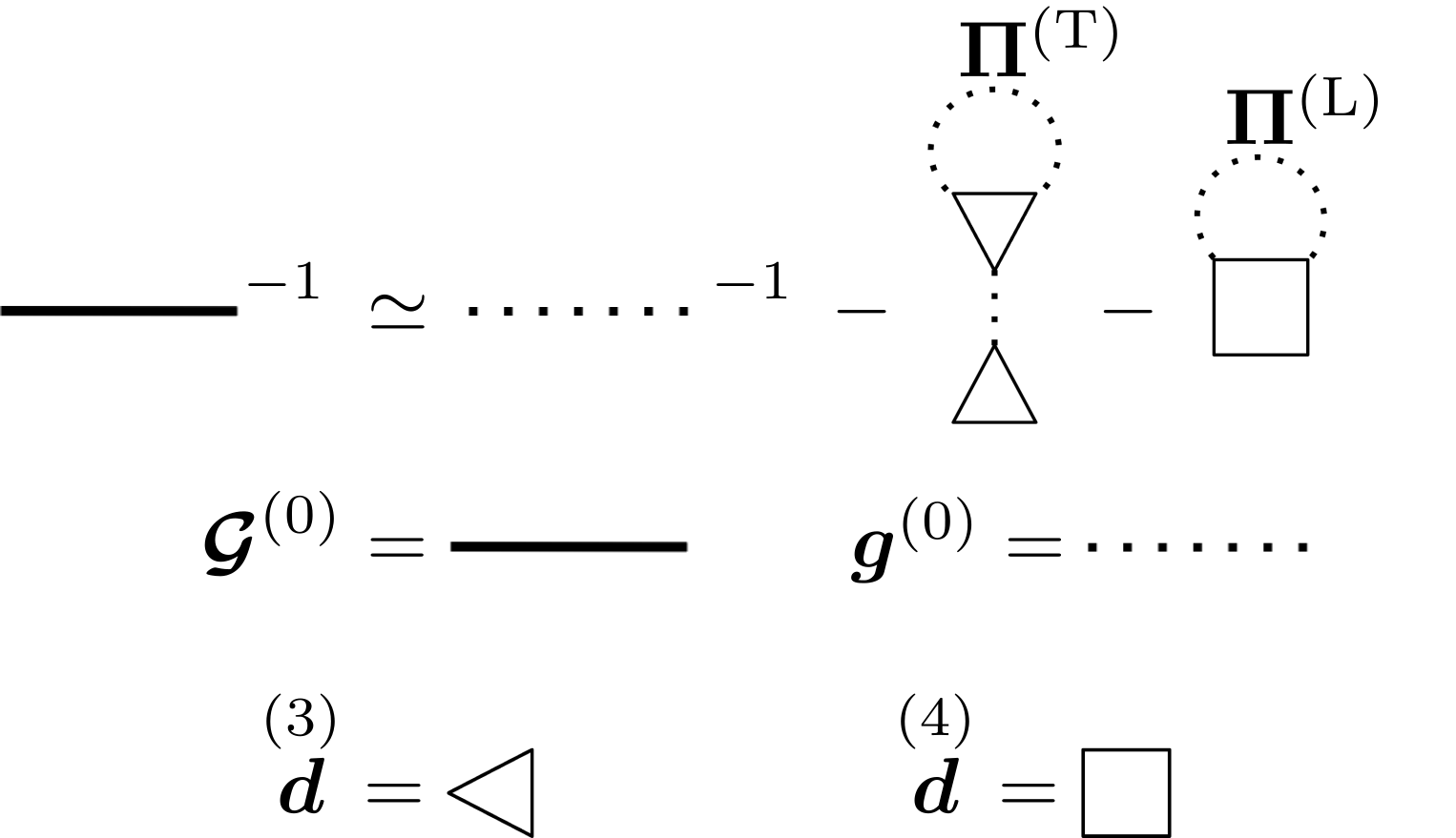
Figure 1: Diagrammatic expression for the SCHA one-phonon propagator at lowest perturbative order $\lambda^{2}$ (see Ref. [46]). The single solid line is the static SCHA propagator $\bm{\mathcal{G}}^{(0)}$ Eq. (29). The thin dotted line is the static harmonic propagator $\bm{g}^{(0)}$ Eq. (30). The scattering vertices are defined in Eq. (34) with $n=3$ (triangle) and $n=4$(square). The tadpole and loop diagram are defined in Eq. (44)

Expressing both the SCHA propagator and the position shift as a series of $\mathcal{O}(\lambda^{n})$ corrections

$$\bm{\mathcal{G}}^{(0)} ={\bm{\mathcal{G}}^{(0)}}^{\lambda=0}+{\bm{\mathcal{G}}^{(0)}}^{\lambda=1}+..\quad{\bm{\mathcal{G}}^{(0)}}^{\lambda=n}\sim\mathcal{O}(\lambda^{n})$$ (42a)

$$\widetilde{\bm{\delta}} =\widetilde{\bm{\delta}}^{\lambda=0}+\widetilde{\bm{\delta}}^{\lambda=1}+..\quad\widetilde{\bm{\delta}}^{\lambda=n}\sim\mathcal{O}(\lambda^{n})$$ (42b)

one can solve order by order in $\lambda$ Eqs (38) (41) (40) to systematically obtain all the corrections to the SCHA propagator with a cubic-quartic potential. Ref. [46] solved Eqs. (38), (41), (40) up to $\mathcal{O}(\lambda^{2})$ and showed that

$$\left(\mathcal{G}^{(0)}\right)^{-1}_{ab}\simeq\left(g^{(0)}\right)^{-1}_{ab}-\left(\Pi^{(\text{L})}_{ab}+\Pi^{(\text{T})}_{ab}\right)$$ (43)

where $\bm{\Pi}^{(\text{L})}$ and $\bm{\Pi}^{(\text{T})}$ are respectively the loop (L) and tadpole (T) diagram (cf. Fig. 1),

$$\Pi^{(\text{L})}_{ab}= -\frac{1}{2}\sum_{cd=1}^{3N}\overset{(4)}{d}_{abcd}g^{(0)}(t=0^{-})_{cd},$$ (44a)

$$\Pi^{(\text{T})}_{ab}= -\frac{1}{2}\sum_{cdef=1}^{3N}\overset{(3)}{d}_{abc}g^{(0)}_{cd}\overset{(3)}{d}_{def}g^{(0)}(t=0^{-})_{ef}\>,$$ (44b)

here $\bm{g}^{(0)}(t=0^{-})$ is the harmonic counterpart of $\bm{\mathcal{G}}^{(0)}(t=0^{-})$, Eq. (39). The loop diagram, Eq. (44a), comes from quantum/anharmonic fluctuations at fixed positions by setting $\widetilde{\bm{\delta}}=\bm{0}$ in Eq. (41). On the other hand, the tadpole diagram, Eq. (44b), comes from the renormalization of atomic positions, Eq. (38).

IV Linear response

The static SCHA corrects the bare phonon propagator with a real self-energy, thus only renormalizing the phonon frequency without introducing a finite lifetime of phonons. In this Section, we revise the fully-dynamical TDSCHA linear response within the Wigner formalism and show how new diagrams with a nonvanishing imaginary part emerge.

IV.1 Linearized equations of motion and general response function

When an external time-dependent potential is coupled to phonons without causing irreversible changes in the material, the system is in the linear response regime. This scenario is relevant, for example, when the ionic degrees of freedom are probed with electromagnetic fields (X-ray or Raman scattering and IR absorption) or with neutrons. In these cases the external perturbation $V^{(\text{ext})}(\bm{R},t)$ is in the form

$$V^{(\text{ext})}(\bm{R},t)=\mathcal{B}(\bm{R})\mathcal{V}(t).$$ (45)

In this regime, the SCHA distribution $\widetilde{\rho}^{(0)}(\bm{R})$ (see Appendix D) is perturbed by $\widetilde{\rho}^{(1)}(\bm{R},t)$

$$\widetilde{\rho}(\bm{R},t)=\widetilde{\rho}^{(0)}(\bm{R})+\widetilde{\rho}^{(1)}(\bm{R},t).$$ (46)

The probability distribution change leads to the emergence of time-dependent correction (denoted by the $(1)$) to the static correlators, Eqs (18),

$$\widetilde{\mathcal{R}}(t)_{\mu} =\widetilde{\mathcal{R}}^{(0)}_{\mu}+\widetilde{\mathcal{R}}^{(1)}_{\mu},$$ (47a)

$$\left\langle\delta\widetilde{R}_{\mu}\delta\widetilde{R}_{\nu}\right\rangle_{\widetilde{\rho}(t)} =\left\langle\delta\widetilde{R}_{\mu}\delta\widetilde{R}_{\nu}\right\rangle_{(0)}+\left\langle\delta\widetilde{R}_{\mu}\delta\widetilde{R}_{\nu}\right\rangle_{(1)},$$ (47b)

$$\left\langle\delta\widetilde{P}_{\mu}\delta\widetilde{P}_{\nu}\right\rangle_{\widetilde{\rho}(t)} =\left\langle\widetilde{P}_{\mu}\widetilde{P}_{\nu}\right\rangle_{(0)}+\left\langle\delta\widetilde{P}_{\mu}\delta\widetilde{P}_{\nu}\right\rangle_{(1)},$$ (47c)

where we express the tensors in the polarization basis $\{\bm{e}_{\mu}\}$ of Eq. (27). In Appendix E, we demonstrate that the dynamics of the average momentum $\small\widetilde{\bm{\mathcal{P}}}^{(1)}$ and of the mixed correlator $\small{\left\langle\delta\widetilde{\bm{R}}\delta\widetilde{\bm{P}}\right\rangle_{(1)}}$ can be reabsorbed in those of the variables of Eqs (47), which define unambiguously the state of the system.

The linearized equations of motion are obtained by plugging the perturbed correlators, Eqs (47), into the equations of motion, Eq. (23), and using Eq. (46) when computing averages of the total potential. This (see Appendix E for details) leads to

$$\left(\bm{\mathcal{L}}^{\prime}+\omega^{2}\right)\cdot\begin{bmatrix}\widetilde{\bm{\mathcal{R}}}^{(1)}\\ \left\langle\delta\widetilde{\bm{R}}\delta\widetilde{\bm{R}}\right\rangle_{(1)}\\ \left\langle\delta\widetilde{\bm{P}}\delta\widetilde{\bm{P}}\right\rangle_{(1)}\end{bmatrix}=\bm{p}^{\prime}\mathcal{V}(\omega),$$ (48)

which defines the linearized TDSCHA equations in frequency domain. In Eq. (48), $\omega^{2}$ comes from the Fourier transform of second-order time derivatives, and $\bm{\mathcal{L}}^{\prime}$ is the linearized Wigner-Liouville operator Eq. (21). In general, we can separate $\bm{\mathcal{L}}^{\prime}$ in two terms

$$\bm{\mathcal{L}}^{\prime}=\bm{\mathcal{L}}^{\prime\dagger}=\bm{\mathcal{L}}^{\prime}_{\text{harm}}+\bm{\mathcal{L}}^{\prime}_{\text{anh}}.$$ (49)

The harmonic part $\bm{\mathcal{L}}^{\prime}_{\text{harm}}$ describes the free evolution of the SCHA phonons defined in Eq. (27). The scattering, hence the interaction between these phonons arises from the anharmonic part $\bm{\mathcal{L}}^{\prime}_{\text{anh}}$. The perturbation vector $\bm{p}^{\prime}$ depends, in general, on equilibrium averages of first and second derivatives of $\mathcal{B}(\bm{R})$.

The external potential modifies the non-interacting equilibrium state, defined by Eq. (25). The response function encodes how the observable $\mathcal{A}(\bm{R})$ changes when the system is out of equilibrium. In the linear response regime, this modification depends only on equilibrium quantities.

The TDSCHA response function is obtained expanding $\small{\left\langle\mathcal{A}\right\rangle_{\widetilde{\rho}^{(0)}+\widetilde{\rho}^{(1)}}}$ (see Eq. (46)) in the perturbed parameters of Eqs (47) around the equilibrium value $\small{\left\langle\mathcal{A}\right\rangle_{(0)}}$. In Appendix E, we show that the first-order correction in the frequency domain is a simple scalar product in the space of the correlators (Eq. (47))

$$\left\langle\mathcal{A}\right\rangle_{(1)}(\omega)=\bm{r}^{\prime\dagger}\cdot\begin{bmatrix}\widetilde{\bm{\mathcal{R}}}^{(1)}\\ \left\langle\delta\widetilde{\bm{R}}\delta\widetilde{\bm{R}}\right\rangle_{(1)}\\ \left\langle\delta\widetilde{\bm{P}}\delta\widetilde{\bm{P}}\right\rangle_{(1)}\end{bmatrix},$$ (50)

where the response vector $\bm{r}^{\prime}$, similarly to $\bm{p}^{\prime}$, contains equilibrium averages of position-derivatives of $\mathcal{A}(\bm{R})$.

Finally, inverting the linearized equations of motion, Eq. (48), we get

$$\left\langle\mathcal{A}\right\rangle_{(1)}(\omega)=\bm{r}^{\prime\dagger}\cdot\left(\bm{\mathcal{L}}^{\prime}+\omega^{2}\right)^{-1}\cdot\bm{p}^{\prime}\mathcal{V}(\omega),$$ (51)

where $\circ^{-1}$ denotes the inverse. The general response function of an observable $\mathcal{A}(\bm{R})$ to an external perturbation $\mathcal{B}(\bm{R})$ is

$$\chi(\omega)_{\mathcal{A},\mathcal{B}}=\bm{r}^{\prime\dagger}\cdot\left(\bm{\mathcal{L}}^{\prime}+\omega^{2}\right)^{-1}\cdot\bm{p}^{\prime}.$$ (52)

This expression has the same form as the one presented in Ref. [25] where the standard description of quantum mechanics is adopted.

In Appendix F we show how to compute the general response function (Eq. (52)) with the Lanczos algorithm following the original work on TDSCHA [25]. The algorithm generates a basis in which $\bm{\mathcal{L}}^{\prime}+\omega^{2}$ is tridiagonal. As shown in Appendix F, from this form it is easy to get in one shot the response function for all values of $\omega$. The Lanczos basis is generated from $N_{\text{steps}}$ sequential applications of $\bm{\mathcal{L}}^{\prime}$ to a starting vector. Each iteration corresponds to free propagations ($\bm{\mathcal{L}}^{\prime}_{\text{harm}}$) and scattering ($\bm{\mathcal{L}}^{\prime}_{\text{anh}}$). In this way, we build the full anharmonic propagators (see next Section IV.2). In addition, we leverage the properties of the Wigner formulation that $\bm{\mathcal{L}}^{\prime}=\bm{\mathcal{L}}^{\prime\dagger}$ and that, if $\mathcal{A}=\mathcal{B}$, $\bm{p}^{\prime}=\bm{r}^{\prime}$. These features imply that a symmetric Lanczos algorithm is sufficient to compute Eq. (52), effectively speeding up the original code by a factor of two [25].

Notation	Diagram	Formula	Description	Eq.
$\mathcal{G}^{(0)}(\omega)_{\mu\nu}$		$\frac{\delta_{\mu\nu}}{\omega^{2}-\omega^{2}_{\mu}}$	Bare one-phonon SCHA propagator	(29)
${g}^{(0)}(\omega)_{\mu\nu}$		$\frac{\delta_{\mu\nu}}{\omega^{2}-\Omega^{2}_{\mu}}$	Bare perturbative one-phonon propagator	(30)
$\chi^{(0)}(\omega)_{\mu\nu\eta\lambda}$		$\chi^{(0)}_{-}(\omega)_{\mu\nu\eta\lambda}-\chi^{(0)}_{+}(\omega)_{\mu\nu\eta\lambda}$	Bare two-phonon SCHA propagator	(72)
$\chi^{(0)}_{-}(\omega)_{\mu\nu\eta\lambda}$		$\delta_{\mu\eta}\delta_{\nu\lambda}\frac{\hbar\left[\omega_{\mu}-\omega_{\nu}\right]\left[n_{\mu}-n_{\nu}\right]}{4\omega_{\mu}\omega_{\nu}[(\omega_{\mu}-\omega_{\nu})^{2}-\omega^{2}]}$	Resonant two-phonon SCHA propagator	(73a)
$\chi^{(0)}_{+}(\omega)_{\mu\nu\eta\lambda}$		$\delta_{\mu\eta}\delta_{\nu\lambda}\frac{\hbar\left[\omega_{\mu}+\omega_{\nu}\right]\left[1+n_{\mu}+n_{\nu}\right]}{4\omega_{\mu}\omega_{\nu}[(\omega_{\mu}+\omega_{\nu})^{2}-\omega^{2}]}$	Antiresonant two-phonon SCHA propagator	(73b)
$\overset{(4)}{D}_{\mu\nu\eta\lambda}$		$\left\langle\frac{\partial^{4}V^{(\text{BO})}}{\partial\widetilde{R}_{\mu}\partial\widetilde{R}_{\nu}\partial\widetilde{R}_{\eta}\partial\widetilde{R}_{\lambda}}\right\rangle_{(0)}$	Four-phonon SCHA scattering vertex	(75)
$\overset{(4)}{D}_{\mu\nu\eta\lambda}{\color[rgb]{1,1,1},}^{(0)}$		$\frac{\partial^{4}V^{\text{(BO)}}}{\partial\widetilde{R}_{\mu}\partial\widetilde{R}_{\nu}\partial\widetilde{R}_{\eta}\partial\widetilde{R}_{\lambda}}\biggl{|}_{\bm{R}=\bm{\mathcal{R}}^{(0)}}$	Perturbative four-phonon scattering vertex evaluated at the SCHA equilibrium positions	(77)
$\overset{(4)}{d}_{\mu\nu\eta\lambda}$		$\frac{\partial^{4}V^{\text{(BO)}}}{\partial\widetilde{R}_{\mu}\partial\widetilde{R}_{\nu}\partial\widetilde{R}_{\eta}\partial\widetilde{R}_{\lambda}}\biggl{|}_{\bm{R}=\bm{\mathcal{R}}_{\text{BO}}}$	Perturbative four-phonon scattering vertex	(34)
$\overset{(3)}{D}_{\mu\nu\eta}$		$\left\langle\frac{\partial^{3}V^{(\text{BO})}}{\partial\widetilde{R}_{\mu}\partial\widetilde{R}_{\nu}\partial\widetilde{R}_{\eta}}\right\rangle_{(0)}$	Three-phonon SCHA scattering vertex	(74)
$\overset{(3)}{D}_{\mu\nu\eta}{\color[rgb]{1,1,1},}^{(0)}$		$\frac{\partial^{3}V^{(\text{BO})}}{\partial\widetilde{R}_{\mu}\partial\widetilde{R}_{\nu}\partial\widetilde{R}_{\eta}}\biggl{|}_{\bm{R}=\bm{\mathcal{R}}^{(0)}}$	Perturbative three-phonon scattering vertex evaluated at SCHA equilibrium positions	(77)
$\overset{(3)}{d}_{\mu\nu\eta}$		$\frac{\partial^{3}V^{(\text{BO})}}{\partial\widetilde{R}_{\mu}\partial\widetilde{R}_{\nu}\partial\widetilde{R}_{\eta}}\biggl{|}_{\bm{R}=\bm{\mathcal{R}}_{\text{BO}}}$	Perturbative three-phonon scattering vertex	(34)

Table 1: Collection of symbols frequently used in the main text. First column: the notation used. Second column: graphical expression with indexes. Third column: mathematical definition. Fourth column: description of the symbol. Fifth column: first labeled equation where the symbol appears.

IV.2 Diagrammatic interpretation of linear response

In this Section, we provide an interpretation in terms of Feynman diagrams of Eq. (52). To do this, we introduce a new basis (see Appendix G and Appendix H for details), a linear combination of the position and momentum correlators, Eqs (47b) (47c). In this basis, the general response function (Eq. (52)) takes the form

$$\chi(\omega)_{\mathcal{A},\mathcal{B}}=\bm{r}\cdot\bm{\mathcal{L}}(\omega)^{-1}\cdot\bm{p},$$ (65)

where the response vector $\bm{r}$ and the perturbation vector $\bm{p}$ have a simple expression in terms of equilibrium averages of $\mathcal{A}(\bm{R})$ and $\mathcal{B}(\bm{R})$

$$\bm{p}=\begin{bmatrix}\left\langle\frac{\partial\mathcal{B}}{\partial\widetilde{R}_{\mu}}\right\rangle_{(0)}\\ \left\langle\frac{\partial^{2}\mathcal{B}}{\partial\widetilde{R}_{\mu}\partial\widetilde{R}_{\nu}}\right\rangle_{(0)}\\ \left\langle\frac{\partial^{2}\mathcal{B}}{\partial\widetilde{R}_{\mu}\partial\widetilde{R}_{\nu}}\right\rangle_{(0)}\end{bmatrix},\qquad\bm{r}=\begin{bmatrix}\left\langle\frac{\partial\mathcal{A}}{\partial\widetilde{R}_{\mu}}\right\rangle_{(0)}\\ \left\langle\frac{\partial^{2}\mathcal{A}}{\partial\widetilde{R}_{\mu}\partial\widetilde{R}_{\nu}}\right\rangle_{(0)}\\ \left\langle\frac{\partial^{2}\mathcal{A}}{\partial\widetilde{R}_{\mu}\partial\widetilde{R}_{\nu}}\right\rangle_{(0)}\end{bmatrix}.$$ (66)

$\bm{\mathcal{L}}(\omega)$ propagates the perturbation caused by $\bm{p}$ in the system and encodes the information on how the latter affects $\bm{r}$ which defines how the observable changes. Indeed, its multiplication by a vector representing the status of the system, as $\bm{r}$ or $\bm{p}$ (Eq. LABEL:perturbation_response_vector), gives the anharmonic scattering processes that further dress the SCHA Green’s function introducing a finite lifetime (see Section IV.3).

In this basis, $\bm{\mathcal{L}}(\omega)$ of Eq. (65) has a simple symmetric form

$$\bm{\mathcal{L}}(\omega)=\begin{bmatrix}\bm{\mathcal{G}}^{(0)}(\omega)^{-1}&-\overset{(3)}{\bm{D}}&-\overset{(3)}{\bm{D}}\\ -\overset{(3)}{\bm{D}}&\bm{\chi}^{(0)}_{-}(\omega)^{-1}-\overset{(4)}{\bm{D}}&-\overset{(4)}{\bm{D}}\\ -\overset{(3)}{\bm{D}}&-\overset{(4)}{\bm{D}}&-\bm{\chi}^{(0)}_{+}(\omega)^{-1}-\overset{(4)}{\bm{D}}\end{bmatrix},$$ (67)

$$\bm{\mathcal{L}}(\omega)=\bm{\mathcal{L}}(\omega)^{\dagger}.$$ (68)

The harmonic and anharmonic contributions to $\bm{\mathcal{L}}(\omega)$ are

$$\bm{\mathcal{L}}_{\text{harm}}(\omega)=\begin{bmatrix}\bm{\mathcal{G}}^{(0)}(\omega)^{-1}&\bm{0}&\bm{0}\\ \bm{0}&\bm{\chi}^{(0)}_{-}(\omega)^{-1}&\bm{0}\\ \bm{0}&\bm{0}&-\bm{\chi}^{(0)}_{+}(\omega)^{-1}\end{bmatrix},$$ (69)

$$\bm{\mathcal{L}}_{\text{anh}}(\omega)=\begin{bmatrix}\bm{0}&-\overset{(3)}{\bm{D}}&-\overset{(3)}{\bm{D}}\\ -\overset{(3)}{\bm{D}}&-\overset{(4)}{\bm{D}}&-\overset{(4)}{\bm{D}}\\ -\overset{(3)}{\bm{D}}&-\overset{(4)}{\bm{D}}&-\overset{(4)}{\bm{D}}\end{bmatrix}.$$ (70)

We report in Fig. 2 a graphical expression for Eq. (67). To construct a diagrammatic representation, we associate each tensor in $\bm{\mathcal{L}}(\omega)$ with a symbol that possesses a number of extremities equal to the rank of the tensor.

Figure 2: Graphical expression for Eq. (67) in terms of the free SCHA propagators (single and double solid line Eqs (71) (72)) and the third and fourth order scattering vertex (orange triangle and red square defined in Eqs (74) (75)).

The single solid line in Fig. 2 represents the equilibrium SCHA Green’s function $\bm{\mathcal{G}}^{(0)}(\omega)$

$$\mathcal{G}^{(0)}(\omega)_{\mu\nu}=\frac{\delta_{\mu\nu}}{\omega^{2}-\omega^{2}_{\mu}},$$ (71)

where $\{\omega_{\mu}\}$ are the self-consistent auxiliary frequencies defined in Eq. (27). The double single solid line in Fig. 2 is the two-phonon SCHA propagator $\bm{\chi}^{(0)}(\omega)$

$$\chi^{(0)}(\omega)_{\mu\nu\eta\lambda}=\chi^{(0)}_{-}(\omega)_{\mu\nu\eta\lambda}-\chi^{(0)}_{+}(\omega)_{\mu\nu\eta\lambda}$$ (72)

which contains a resonant $\bm{\chi}^{(0)}_{-}(\omega)$ and an anti resonant term $\bm{\chi}^{(0)}_{+}(\omega)$

$$\chi^{(0)}_{-}(\omega)_{\mu\nu\eta\lambda}= \delta_{\mu\eta}\delta_{\nu\lambda}\frac{\hbar\left[\omega_{\mu}-\omega_{\nu}\right]\left[n_{\mu}-n_{\nu}\right]}{4\omega_{\mu}\omega_{\nu}[(\omega_{\mu}-\omega_{\nu})^{2}-\omega^{2}]},$$ (73a)

$$\chi^{(0)}_{+}(\omega)_{\mu\nu\eta\lambda}= \delta_{\mu\eta}\delta_{\nu\lambda}\frac{\hbar\left[\omega_{\mu}+\omega_{\nu}\right]\left[1+n_{\mu}+n_{\nu}\right]}{4\omega_{\mu}\omega_{\nu}[(\omega_{\mu}+\omega_{\nu})^{2}-\omega^{2}]}.$$ (73b)

The anti resonant part $\bm{\chi}^{(0)}_{+}(\omega)$ describes the absorption/emission processes of a phonon pair (double solid line with both arrows in the same directions in Fig. 2) while the resonant $\bm{\chi}^{(0)}_{-}(\omega)$ the case in which one phonon is absorbed and the other one is emitted (double solid line with arrows pointing in opposite directions in Fig. 2).

The first row of Eq. (67) relates the propagation of single phonon excitation $\bm{\mathcal{G}}^{(0)}(\omega)$ to two-phonon processes $\bm{\chi}^{(0)}_{\pm}(\omega)$. This is mediated by the three-phonon scattering vertex (orange triangle of Fig. 2)

$$\overset{(3)}{D}_{\mu\nu\eta}=\left\langle\frac{\partial^{3}V^{(\text{BO})}}{\partial\widetilde{R}_{\mu}\partial\widetilde{R}_{\nu}\partial\widetilde{R}_{\eta}}\right\rangle_{(0)}.$$ (74)

The second and third rows of Eq. (67) show that double excitations interact with each other via the fourth-order scattering vertex (red square of Fig. 2)

$$\overset{(4)}{D}_{\mu\nu\eta\lambda}=\left\langle\frac{\partial^{4}V^{(\text{BO})}}{\partial\widetilde{R}_{\mu}\partial\widetilde{R}_{\nu}\partial\widetilde{R}_{\eta}\partial\widetilde{R}_{\lambda}}\right\rangle_{(0)},$$ (75)

or can decay in a single phonon via the three-phonon scattering vertex, Eq. (74). As a guide for the reader, in Table 1 we report a summary of all the symbols used.

So, by just looking at the expression of $\bm{\mathcal{L}}(\omega)$, we understand that in TDSCHA only single and double excitation are dressed by anharmonicity and that only single phonons can decay in a higher-order phonon propagation.

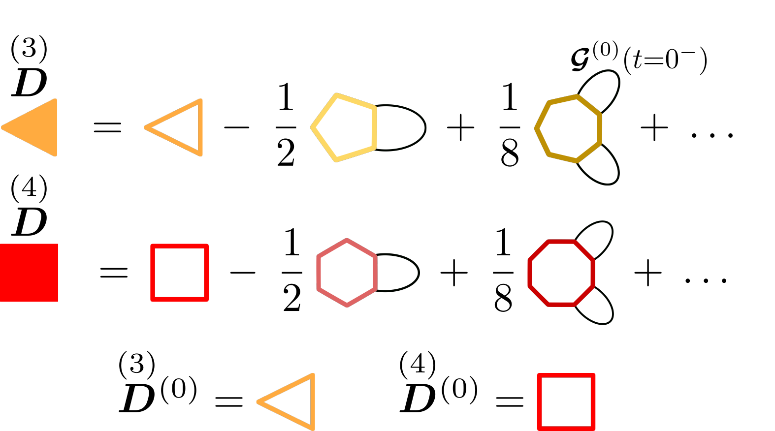
Figure 3: Diagrammatic expression for the SCHA scattering tensors Eqs (74) (75) as presented in Eqs (76). Each SCHA propagator is contracted with a higher order derivative of the anharmonic tensor Eq. (77) which are evaluated at the SCHA positions, i.e. they do not coincide with Eq. (34). These are represented as $n=3,5,7..$ and $n=4,6,8..$ regular polygons.

The scattering vertices, Eqs (74) (75), included in the dynamical response have an interesting diagrammatic expression (see also Ref. [51]). In general, they do not coincide with the derivatives of the BO potential evaluated at the equilibrium SCHA positions $\small\bm{\mathcal{R}}^{(0)}$ but they contain extra terms due to quantum-thermal fluctuations. All of these terms are included in the TDSCHA. Expanding Eqs (74) (75) in $\small\bm{R}-\small\bm{\mathcal{R}}^{(0)}$, we get the following series, as reported in Appendix I,

$$\overset{(3)}{D}_{\mu\nu\eta}= \sum_{n=0}^{+\infty}\frac{(-1)^{n}}{2^{n}n!}\sum_{\alpha_{1}..\alpha_{2n}=1}^{3N}\overset{(3+2n)}{D}_{\mu\nu\eta\alpha_{1}..\alpha_{2n-1}\alpha_{2n}}{\color[rgb]{1,1,1},}^{(0)}$$

$$\mathcal{G}^{(0)}(t=0^{-})_{\alpha_{1}\alpha_{2}}..\mathcal{G}^{(0)}(t=0^{-})_{\alpha_{2n-1}\alpha_{2n}},$$ (76a)

$$\overset{(4)}{D}_{\mu\nu\eta\lambda}= \sum_{n=0}^{+\infty}\frac{(-1)^{n}}{2^{n}n!}\sum_{\alpha_{1}..\alpha_{2n}=1}^{3N}\overset{(4+2n)}{D}_{\mu\nu\eta\lambda\alpha_{1}\alpha_{2}..\alpha_{2n-1}\alpha_{2n}}{\color[rgb]{1,1,1},}^{(0)}$$

$$\mathcal{G}^{(0)}(t=0^{-})_{\alpha_{1}\alpha_{2}}..\mathcal{G}^{(0)}(t=0^{-})_{\alpha_{2n-1}\alpha_{2n}},$$ (76b)

where the anharmonic vertices in the series are

$$\overset{(n)}{D}_{\alpha_{1}..\alpha_{n}}{\color[rgb]{1,1,1},}^{(0)}\quad=\frac{\partial^{n}V^{\text{(BO)}}}{\partial\widetilde{R}_{\alpha_{1}}..\partial\widetilde{R}_{\alpha_{n}}}\biggl{|}_{\bm{R}=\bm{\mathcal{R}}^{(0)}}.$$ (77)

These differ in general from $\overset{(n)}{\bm{d}}$, see Eq. (34), since the minimum of the Born-Oppenheimer potential $\bm{\mathcal{R}}_{\text{BO}}$ does not coincide with the SCHA centroid $\bm{\mathcal{R}}^{(0)}$. In Fig. 3 we report the diagrammatic expansion for Eqs (76). Each anharmonic tensor in Eq. (77) with $n>3,4$ has a pair of indexes contracted with a SCHA propagator $\bm{\mathcal{G}}^{(0)}(t=0^{-})$ (Eq. (77)). This indicates that quantum-thermal fluctuations result in the renormalization of the anharmonic vertices.

IV.3 Anharmonic propagators

In this Section, we discuss the TDSCHA interacting propagators. Specifically, we present two-phonon processes that have been neglected in previous works [25, 26].

In TDSCHA, the one-phonon $\mathcal{G}(\omega)_{\mu\nu}$, two-phonon $\chi(\omega)_{\mu\nu\eta\lambda}$, and the one-two phonon $\Gamma(\omega)_{\mu\eta\lambda}$ interacting propagators are obtained as response functions by setting in $\chi(\omega)_{\mathcal{A},\mathcal{B}}$ (Eq. (65))

$$\mathcal{A}_{\mathcal{G}}=\delta\widetilde{R}^{(0)}_{\mu} \mathcal{B}_{\mathcal{G}}= \delta\widetilde{R}^{(0)}_{\nu},$$ (78a)

$$\mathcal{A}_{\chi}=\frac{1}{2}\delta\widetilde{R}^{(0)}_{\mu}\delta\widetilde{R}^{(0)}_{\nu} \mathcal{B}_{\chi}= \frac{1}{2}\delta\widetilde{R}^{(0)}_{\eta}\delta\widetilde{R}^{(0)}_{\lambda},$$ (78b)

$$\mathcal{A}_{\Gamma}=\delta\widetilde{R}^{(0)}_{\mu} \mathcal{B}_{\Gamma}= \frac{1}{2}\delta\widetilde{R}^{(0)}_{\eta}\delta\widetilde{R}^{(0)}_{\lambda}.$$ (78c)

The response and perturbation vectors (see Eqs (LABEL:perturbation_response_vector)) corresponding to Eqs (78) are as follows

$$\bm{r}_{\mathcal{G}}= \begin{bmatrix}\bm{\delta}_{\mu}\\ \bm{0}\\ \bm{0}\end{bmatrix} \bm{p}_{\mathcal{G}}=\begin{bmatrix}\bm{\delta}_{\nu}\\ \bm{0}\\ \bm{0}\end{bmatrix},$$ (79a)

$$\bm{r}_{\chi}= \begin{bmatrix}\bm{0}\\ \bm{S}_{\mu\nu}\\ \bm{S}_{\mu\nu}\end{bmatrix} \bm{p}_{\chi}=\begin{bmatrix}\bm{0}\\ \bm{S}_{\eta\lambda}\\ \bm{S}_{\eta\lambda}\end{bmatrix},$$ (79b)

$$\bm{r}_{\Gamma}= \begin{bmatrix}\bm{\delta}_{\mu}\\ \bm{0}\\ \bm{0}\end{bmatrix} \bm{p}_{\Gamma}=\begin{bmatrix}\bm{0}\\ \bm{S}_{\eta\lambda}\\ \bm{S}_{\eta\lambda}\end{bmatrix},$$ (79c)

where $\bm{\delta}_{\mu}$ is a $3N$ vector with 1 in the mode index $\mu$ and zero elsewhere and $\bm{S}_{\eta\lambda}$ is a $3N\times 3N$ matrix with $1/2$ on the mode indexes $\eta$ and $\lambda$ and zeros elsewhere.

The choice of $\mathcal{A}/\mathcal{B}$, as in Eqs (78), is not arbitrary. In the non-interacting case, $\bm{\mathcal{L}}(\omega)$ is diagonal, so the response function simplifies to

$$\chi(\omega)_{\mathcal{A},\mathcal{B}}= \bm{r}_{i}\begin{bmatrix}\bm{\mathcal{G}}^{(0)}(\omega)&\bm{0}&\bm{0}\\ \bm{0}&\bm{\chi}^{(0)}_{-}(\omega)&\bm{0}\\ \bm{0}&\bm{0}&-\bm{\chi}^{(0)}_{+}(\omega)\end{bmatrix}\bm{p}_{i}$$ (80)

$$i= \mathcal{G},\mathcal{\chi},\Gamma.$$

From Eq. (80) we recover the one and two phonon free propagators (Eqs (71) (72)) and no cross terms connecting single to double excitations. These results are consistent with the standard linear response theory, in the non-interacting case, treated with the many-body formalism. This shows that Eqs (79) recover physically relevant quantities.

To get the interacting Green’s function, we plug $\bm{r}$ and $\bm{p}$ of Eqs (79) in the expression of $\chi(\omega)_{\mathcal{A},\mathcal{B}}$, Eq. (65), and we invert $\bm{\mathcal{L}}(\omega)$ following Refs [25, 52, 53] (see also Appendix G). To do this, we consider $\bm{\mathcal{L}}(\omega)$, Eq. (67), as a $3\times 3$ block-matrix (as represented in Fig. 2) where each block itself is a tensor. The same applies to $\bm{r}$ and $\bm{p}$, Eqs (LABEL:perturbation_response_vector), which are understood as $3$ components vectors. From the non-interacting case (Eq. (80)), we learn that the first component of $\bm{p}/\bm{r}$ controls the single-mode propagation while the second and third the two-phonon channel.

The inversion process mixes the matrix elements of $\bm{\mathcal{L}}(\omega)$ adding interactions to the free propagators which are expressed as diagrammatic series. The representation of Fig. 2 is a graphical aid to visualize the building blocks of these diagrams. In Appendix H we report the details of all the results presented.

In our calculations we always reduce the inversion of $\bm{\mathcal{L}}(\omega)$ to a $2\times 2$ block-matrix with the following form

$$\begin{bmatrix}\bm{A}&\bm{C}\\ \bm{C}^{\dagger}&\bm{B}\end{bmatrix}$$ (81)

which can be easily inverted (see Appendix G)

$$\small\begin{bmatrix}\bm{D}^{-1}&\quad-\bm{D}^{-1}\cdot\bm{C}\cdot\bm{B}^{-1}\\ -\bm{B}^{-1}\cdot\bm{C}^{\dagger}\cdot\bm{D}^{-1}&\quad\bm{B}^{-1}\cdot\left(\bm{1}+\bm{C}^{\dagger}\cdot\bm{D}^{-1}\cdot\bm{C}\cdot\bm{B}^{-1}\right)\end{bmatrix}$$ (82)

where $\bm{D}=\bm{A}-\bm{C}\cdot\bm{B}^{-1}\cdot\bm{C}^{\dagger}$.

First, we discuss the one-phonon propagator. Because only the first component of both $\bm{p}_{\mathcal{G}}$ and $\bm{r}_{\mathcal{G}}$, Eq. (79a), are non-zero, the response calculation is simplified. In particular, we compact the $2\times 2$ two-phonon sector of $\bm{\mathcal{L}}(\omega)$ (i.e. $\bm{\mathcal{L}}(\omega)_{ij}$ with $i,j>1$) in a $1\times 1$ block matrix. As shown in Appendix H, $\bm{\mathcal{L}}(\omega)$ is reduced to a $2\times 2$ block-matrix $\bm{\mathcal{L}}_{\text{1ph}}(\omega)$, so that the one-phonon propagator is given by

$$\bm{\mathcal{G}}(\omega)= \bm{r}_{\mathcal{G}}\cdot\bm{\mathcal{L}}(\omega)^{-1}\cdot\bm{p}_{\mathcal{G}}=\left(\bm{\mathcal{L}}_{\text{1ph}}(\omega)^{-1}\right)_{11}$$ (83)

where

$$\bm{\mathcal{L}}_{\text{1ph}}(\omega)=\begin{bmatrix}\bm{\mathcal{G}}^{(0)}(\omega)^{-1}&-\overset{(3)}{\bm{D}}\\ -\overset{(3)}{\bm{D}}&\bm{\chi}^{(0)}(\omega)^{-1}-\overset{(4)}{\bm{D}}\end{bmatrix}.$$ (84)

Note that $\left(\bm{\mathcal{L}}_{\text{1ph}}(\omega)\right)_{22}$ represents the anharmonic two-phonon channel in which single modes can decay through the three-phonon vertex, $\left(\bm{\mathcal{L}}_{\text{1ph}}(\omega)\right)_{12}$. Graphically Eq. (83) corresponds to

$$\begin{split}\includegraphics[width=34.69038pt,valign={c}]{SIMBOLI/G.png}&=\matrixquantity[\includegraphics[width=21.68231pt,valign={c}]{SIMBOLI/G0.png}^{-1}\hfil&-\includegraphics[height=14.22636pt,valign={c}]{SIMBOLI/d3.png}\\ -\scalebox{-1.0}[1.0]{\includegraphics[height=14.22636pt,valign={c}]{SIMBOLI/d3.png} }&\includegraphics[width=28.45274pt,valign={c}]{SIMBOLI/chi0.png}^{-1}-\includegraphics[height=14.22636pt,valign={c}]{SIMBOLI/d4.png}]^{-1}_{\>\>11}.\end{split}$$ (85)

In Eq. (83) we apply the general result of Eq. (82) to obtain the interacting Green’s function

$$\bm{\mathcal{G}}(\omega)=\bm{\mathcal{G}}^{(0)}(\omega)+\bm{\mathcal{G}}^{(0)}(\omega)\cdot\bm{\Pi}(\omega)\cdot\bm{\mathcal{G}}(\omega),$$ (86)

where the self-energy $\bm{\Pi}(\omega)$ coincides with the one reported in Refs [25, 26, 46]

$$\bm{\Pi}(\omega)=\overset{(3)}{\bm{D}}:\left(\bm{1}-\bm{\chi}^{(0)}(\omega):\overset{(4)}{\bm{D}}\right)^{-1}:\bm{\chi}^{(0)}(\omega):\overset{(3)}{\bm{D}},$$ (87)

here $\small{\bm{A}:\bm{B}=\sum_{\mu\nu=1}^{3N}A_{..\mu\nu}B_{\mu\nu..}}$. Our definition of the non-interacting two-phonon propagator $\bm{\chi}^{(0)}(\omega)$ (Eq. (72)) is one reported by Ref. [46] in Eq. (72) multiplied by $-1/2$ so that all the definitions are consistent.

Physical phonon frequencies and lifetimes are determined by real and imaginary parts of $\bm{\mathcal{G}}(\omega+i0^{+})$, Eq. (86), as discussed in Ref. [42]. In addition, we remark that the polarization vectors can also change when adding dynamical effects so polarization-mixing is automatically included in Eq. (86).

The bubble diagram is the lowest-order approximation for the self-energy, as described in Eq. (87), and is incorporated in many self-consistent phonon (SCP) calculations within the improved SCP (ISCP) framework [37, 54, 55, 56]. TDSCHA represents a theoretical approach that justifies this from the least action principle and provides a path to move beyond the bubble approximation.

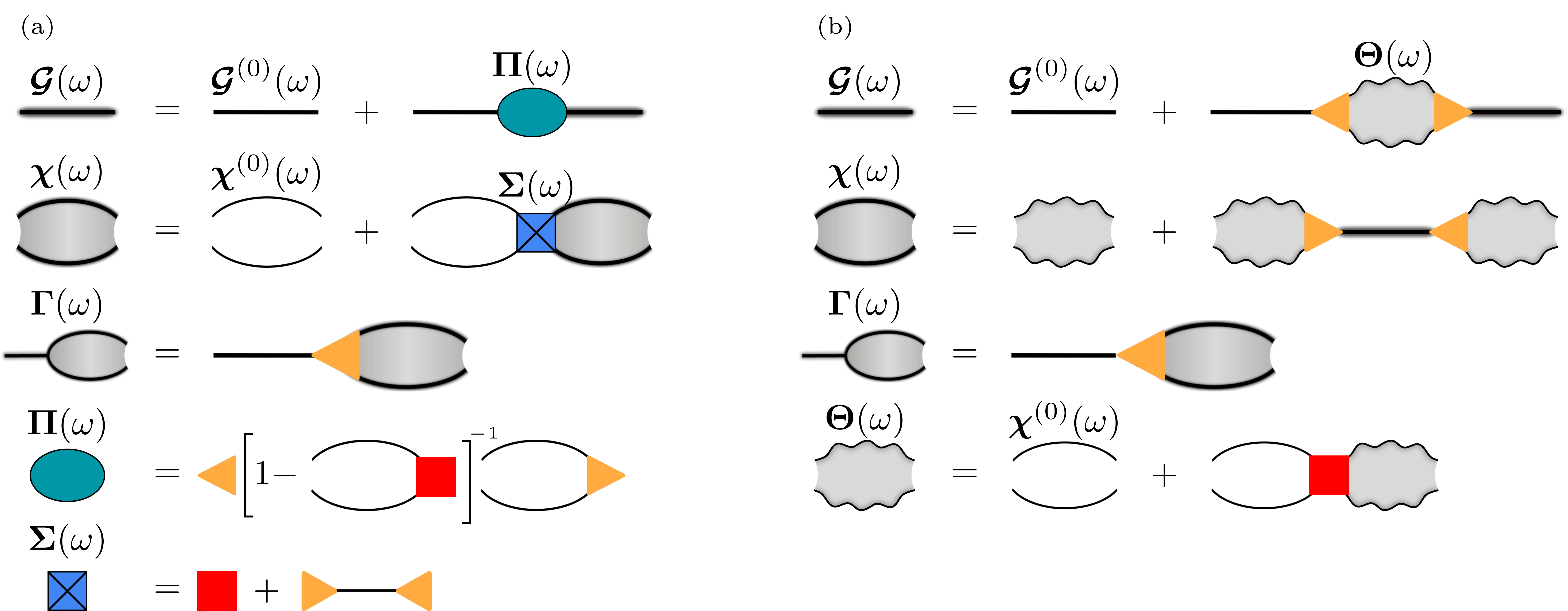
Figure 4: In a) we report the diagrammatic expression of the interacting one, two and one-two phonon Green’s functions, Eqs (86) (92) (93). In b) we show Eqs (94). Thinner solid lines represent the non-interacting SCHA propagators $\bm{\mathcal{G}}^{(0)}(\omega)$ and $\bm{\chi}^{(0)}(\omega)$, defined in Eqs (86) (92). The three/four-phonon scattering vertices are defined in Eqs (74) (75) and represented as orange triangles and red squares.

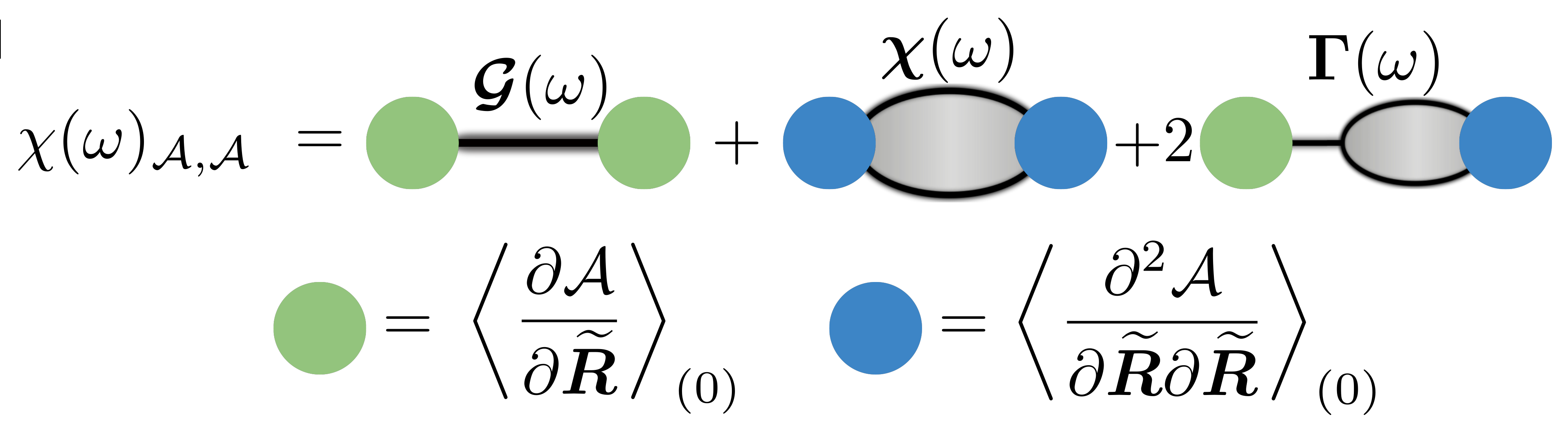
Figure 5: Diagrammatic expression of the processes included in the fully interacting response, Eq. (65), if $\mathcal{A}=\mathcal{B}$. The interacting TDSCHA Green’s functions are reported in Eqs (86) (92) (93). The green vertex is related to the first entry of $\bm{p}$/$\bm{r}$ while the blue vertex to the second and third entries of $\bm{p}$/$\bm{r}$, see Eqs. (LABEL:perturbation_response_vector).

For the two-phonon case, we proceed as before. We use the definition of $\bm{r}_{\chi}/\bm{p}_{\chi}$ (Eq. (79b)) to reabsorb the one-phonon sector of $\bm{\mathcal{L}}(\omega)$ (i.e. the row $\bm{\mathcal{L}}(\omega)_{1j}$ and column $\bm{\mathcal{L}}(\omega)_{j1}$ with $j=1,2,3$) into the two-phonon sector. So we solve

$$\bm{\chi}(\omega)=\bm{r}_{\chi}\cdot\bm{\mathcal{L}}(\omega)^{-1}\cdot\bm{p}_{\chi}=\sum_{ij}^{1,2}\left(\bm{\mathcal{L}}_{\text{2ph}}(\omega)^{-1}\right)_{ij}$$ (88)

where $\bm{\mathcal{L}}_{\text{2ph}}(\omega)$ is a $2\times 2$ block-matrix

$$\bm{\mathcal{L}}_{\text{2ph}}(\omega)=\begin{bmatrix}\bm{\chi}^{(0)}_{-}(\omega)^{-1}-\bm{\Sigma}(\omega)&-\bm{\Sigma}(\omega)\\ -\bm{\Sigma}(\omega)&-\bm{\chi}^{(0)}_{+}(\omega)^{-1}-\bm{\Sigma}(\omega)\end{bmatrix}.$$ (89)

$\bm{\Sigma}(\omega)$ is the two-phonon self-energy

$$\bm{\Sigma}(\omega)=\bm{\Sigma}(\omega)^{\dagger}=\overset{(4)}{\bm{D}}+\overset{(3)}{\bm{D}}\cdot\bm{\mathcal{G}}^{(0)}(\omega)\cdot\overset{(3)}{\bm{D}}$$ (90)

where single phonon excitations enter in $\bm{\Sigma}(\omega)$ via the three-phonon vertex.

Graphically, Eq. (88) corresponds to

$$\begin{split}\includegraphics[width=42.67912pt,keepaspectratio,valign={c}]{SIMBOLI/chi.png}&=\sum_{ij}^{1,2}\matrixquantity[\includegraphics[width=28.45274pt,keepaspectratio,valign={c}]{SIMBOLI/chi0res.png}^{-1}-\includegraphics[width=14.22636pt,keepaspectratio,valign={c}]{SIMBOLI/sigmathin.png}\hfil&-\includegraphics[width=14.22636pt,keepaspectratio,valign={c}]{SIMBOLI/sigmathin.png}\\ -\includegraphics[width=14.22636pt,keepaspectratio,valign={c}]{SIMBOLI/sigmathin.png}&-\includegraphics[width=28.45274pt,keepaspectratio,valign={c}]{SIMBOLI/chi0ares.png}^{-1}-\includegraphics[width=14.22636pt,keepaspectratio,valign={c}]{SIMBOLI/sigmathin.png}]^{-1}_{ij}\\ \bm{\Sigma}(\omega)&=\includegraphics[width=14.22636pt,keepaspectratio,valign={c}]{SIMBOLI/sigmathin.png}=\includegraphics[width=14.22636pt,keepaspectratio,valign={c}]{SIMBOLI/d4.png}+\includegraphics[height=14.22636pt,keepaspectratio,valign={c}]{SIMBOLI/manubrio.png}.\end{split}$$ (91)

Again we use Eq. (82) to invert Eq. (89) and we end up with the interacting two-phonon propagator

$$\bm{\chi}(\omega)=\bm{\chi}^{(0)}(\omega)+\bm{\chi}^{(0)}(\omega):\bm{\Sigma}(\omega):\bm{\chi}(\omega)$$ (92)

with $\bm{\Sigma}(\omega)$, Eq. (90), being the TDSCHA two-phonon self-energy. We find that, in the two-phonon propagation, there is the possibility of either decay in a single phonon through the third-order scattering vertex or in another pair through the fourth-order scattering vertex. There are no high-order decay processes.

For the mixed propagator, we proceed as before. The form of $\bm{p}_{\Gamma}/\bm{r}_{\Gamma}$ (Eq. (79c)) allows single phonon excitations to be triggered by two-phonon propagation via the three-phonon vertex, leading to a non-zero one-two phonon propagation

$$\bm{\Gamma}(\omega)=\bm{\mathcal{G}}^{(0)}(\omega)\cdot\overset{(3)}{\bm{D}}:\bm{\chi}(\omega).$$ (93)

We demonstrate that Eqs. (86) (92) are the fundamental components of the TDSCHA response. The relationship between these two propagators becomes clear when expressed in terms of the partially screened two-phonon propagator $\bm{\Theta}(\omega)=\bm{\chi}(\omega)\evaluated{}_{\overset{(3)}{\bm{D}}=0}$ in which a phonon pair propagates only through the four phonon scattering vertex. Note that $\bm{\Theta}(\omega)$ generalizes in the dynamical regime Eq. (26) of Ref. [46]. As proved in Appendix H, the new expressions for the propagators are

$$\bm{\mathcal{G}}(\omega) =\bm{\mathcal{G}}^{(0)}(\omega)+\bm{\mathcal{G}}^{(0)}(\omega)\cdot\overset{(3)}{\bm{D}}:\bm{\Theta}(\omega):\overset{(3)}{\bm{D}}\cdot\bm{\mathcal{G}}(\omega),$$ (94a)

$$\bm{\chi}(\omega) =\bm{\Theta}(\omega)+\bm{\Theta}(\omega):\overset{(3)}{\bm{D}}\cdot\bm{\mathcal{G}}(\omega)\cdot\overset{(3)}{\bm{D}}:\bm{\Theta}(\omega),$$ (94b)

$$\bm{\Theta}(\omega) =\bm{\chi}^{(0)}(\omega)+\bm{\chi}^{(0)}(\omega):\overset{(4)}{\bm{D}}:\bm{\Theta}(\omega).$$ (94c)

Now, only $\bm{\mathcal{G}}(\omega)$ and $\bm{\Theta}(\omega)$ have a Dyson form, whereas $\bm{\chi}(\omega)$ has a different structure where single and double propagations are disentangled.

Fig. 4 summarizes the diagrammatic expressions for the interacting propagators. In panel a) we report Eqs (86) (92) (93), while panel b) shows Eqs (94).

By computing all the TDSCHA interacting propagators, we gain a full comprehension of the diagrammatic expression, Fig. 5, introduced in Ref. [25] for the TDSCHA response function $\chi(\omega)_{\mathcal{A},\mathcal{A}}$ (Eq. (65)). In fact, Eq. (65) can be decomposed into the interacting propagators.

One-phonon processes $\bm{\mathcal{G}}(\omega)$ are coupled to first-order position derivatives of the perturbation, first entry of $\bm{p}$/$\bm{r}$ Eqs (LABEL:perturbation_response_vector). On the other hand, two-phonon excitations $\bm{\chi}(\omega)$ and $\bm{\Gamma}(\omega)$ are triggered by non-zero second-order position derivatives of the perturbation, second and third entries of $\bm{p}$/$\bm{r}$ Eqs. (LABEL:perturbation_response_vector).

We emphasize that the Lanczos algorithm includes the effect of the third and fourth-order scattering vertex, Eqs (74) (75), in a non-perturbative way [8] (see Appendix F). TDSCHA evolves ab-initio all the phonon modes in a given supercell without free parameters. This feature is interesting for applications in non-linear phononics where is crucial to comprehend relaxation pathways of coherent phonon oscillations [24, 57, 58, 59].

IV.3.1 Momentum Green function

In Wigner-TDSCHA, the ionic momentum is controlled directly, which was not possible in the original formulation. Here we discuss the TDSCHA momentum-momentum Green’s function $\small\bm{\mathcal{G}}_{\text{p}}(\omega)$. In our theory, this is computed setting

$$\mathcal{A}=\widetilde{P}_{\mu}\quad\mathcal{B}=\widetilde{P}_{\nu}.$$ (95)

The SCHA momentum Green’s function $\bm{\mathcal{G}}^{(0)}_{\text{p}}(\omega)$ is proportional to $\bm{\mathcal{G}}^{(0)}(\omega)$ (Eq. (86)) since the equation for position and momentum are coupled

$$i\omega\widetilde{\bm{\mathcal{P}}}(\omega)=\widetilde{\bm{\mathcal{R}}}(\omega)\longrightarrow\mathcal{G}^{(0)}_{\text{p}}(\omega)_{\mu\nu}=\omega_{\mu}^{2}\mathcal{G}^{(0)}(\omega)_{\mu\nu}.$$ (96)

The free propagators are the building blocks for the interacting theory. Hence the interacting momentum Green’s function $\bm{\mathcal{G}}_{\text{p}}(\omega)$ satisfies a perturbative expansion that is proportional to the one of $\bm{\mathcal{G}}(\omega)$ once the TDSCHA diagrams are selected, i.e. those from Eq. (86). So we have that, see Appendix J for details,

$$\bm{\mathcal{G}}_{\text{p}}(\omega)=-\bm{1}+\omega^{2}\bm{\mathcal{G}}(\omega).$$ (97)

Thus, a Lanczos calculation also provides access to the TDSCHA momentum Green’s function.

IV.4 Multiple excitations in TDSCHA

The Gaussian approximation defines a hierarchy of diagrams that is truncated at the two-phonon level. In this Section, we demonstrate that, in TDSCHA, all higher-order phonon propagators are related to the Green’s functions of Eqs (86) (92) (93).

For example, the three-phonon propagator is obtained setting in Eq. (65) a tensor-like perturbation/response functions

$$\mathcal{A}=\delta\widetilde{R}^{(0)}_{\alpha}\delta\widetilde{R}^{(0)}_{\beta}\delta\widetilde{R}^{(0)}_{\gamma}\qquad\mathcal{B}=\delta\widetilde{R}^{(0)}_{\mu}\delta\widetilde{R}^{(0)}_{\nu}\delta\widetilde{R}^{(0)}_{\eta}.$$ (98)

In this case, only the first entries of $\bm{p}/\bm{r}$, i.e. $\small\left\langle\partial\mathcal{A}/\partial\widetilde{\bm{R}}\right\rangle_{(0)}$, are non-zero. This means that in the case of Eq. (98) we have a one-phonon response, as the one obtained for $\bm{\mathcal{G}}(\omega)$ (Eq. (79a)). As computed in Appendix H, the three-phonon response is

$$\chi_{\mu\nu\eta}^{\alpha\beta\gamma}(\omega)=\mathcal{G}^{(0)}(t=0^{-})_{\beta\gamma}\mathcal{G}^{(0)}(t=0^{-})_{\nu\eta}\mathcal{G}(\omega)_{\alpha\mu}$$ (99)

$$+\text{permutations of $(\alpha\beta\gamma)$ and $(\mu\nu\eta)$}$$

and in Fig. 6 we report its diagrammatic structure. This contains the one-phonon Green’s function $\bm{\mathcal{G}}(\omega)$, Eq. (86), and a disconnected part, $\bm{\mathcal{G}}^{(0)}(t=0^{-})$ which comes from the averages $\left\langle\delta\widetilde{\bm{R}}\delta\widetilde{\bm{R}}\right\rangle_{(0)}$ (Eq. (39)) in $\small\left\langle\partial\mathcal{A}/\partial\widetilde{\bm{R}}\right\rangle_{(0)}$.

Figure 6: Diagrammatic expression for the TDSCHA interacting three-phonon Green’s function obtained as a response to a cubic perturbation, Eq. (98). In TDSCHA, the tree-phonons propagator is a disconnected diagram.

In this case, the SCHA correction, $\bm{\mathcal{G}}^{(0)}(t=0^{-})$, does not enter the phonon propagation but it dresses the interaction with the external probe. This means that if we take a scalar perturbation

$$\mathcal{A}=\mathcal{B}=\frac{1}{3}\sum_{\alpha\beta\gamma=1}^{3N}K_{\alpha\beta\gamma}\delta\widetilde{R}^{(0)}_{\alpha}\delta\widetilde{R}^{(0)}_{\beta}\delta\widetilde{R}^{(0)}_{\gamma},$$ (100)

with $K_{\alpha\beta\gamma}$ a tensor that does not depend on atomic positions, $\bm{\mathcal{G}}^{(0)}(t=0^{-})$ is contracted with $\bm{K}$.

Similarly, all the higher-order propagators, i.e. those obtained with

$$\mathcal{A}\sim\left(\delta\widetilde{R}^{(0)}\right)^{n-2}\quad\mathcal{B}\sim\left(\delta\widetilde{R}^{(0)}\right)^{m-2}\quad m,n>2,$$ (101)

give disconnected diagrams. In all these cases we will get a $\chi_{\mathcal{A},\mathcal{B}}(\omega)$ that contains only one of the TDSCHA propagators (Eqs (86) (92) (93)) along with a disconnected part that depends only on $\bm{\mathcal{G}}^{(0)}(t=0^{-})$, Eq. (39).

Figure 7: Diagrammatic expression for the Saturn diagram with a three SCHA phonon propagation (solid lines are the propagators of Eq. (71)). The red vertex is the four-phonon scattering vertex Eq. (75) which leads to three phonon excitations. This class of diagrams is missed by TDSCHA where we can not connect a single SCHA line to the four-phonon scattering vertex.

So TDSCHA can not capture processes beyond a two-phonon mechanism: the propagators of Eqs (86) (92) (93) serve as the building blocks of the response. This means that there are general rules in the symbolic inversion of $\bm{\mathcal{L}}(\omega)$ (see Eq. (67)). In Fig. 2 the solid line (one-phonon SCHA propagator of Eq. (72)) is always attached to one extremity of the orange triangle (Eq. (74)). The double solid line (two-phonon SCHA propagator Eq. (72)) is connected to two extremities either of the red square (four phonon vertex Eq. (75)) or of the orange triangle (three phonon vertex Eq. (74)).

We do not get three or more SCHA phonon resonances. One example is the ’Saturn’ diagram (Fig. 7) which is missed by our method. This diagram would correspond to a single SCHA propagator attached to the four-phonon vertex and this is not contained in TDSCHA.

Notably, the TDSCHA diagrams arise from the stationary action principle of quantum mechanics [25], ensuring that there is no double counting and that the theory is consistent. The inclusion of new scattering mechanisms, such as Fig. 7, must be approached with extreme care to avoid compromising the internal coherence and overcounting some anharmonic processes.

V Nonlinear phonon-photon coupling: Infrared and Raman

In this section, we provide an overview of the infrared (IR) and Raman response in TDSCHA, with a particular emphasis on the two-phonon effect.

IR experiments involve the absorption of infrared light by normal modes, which are associated with a variation in dipole moment and, in crystals, these are optical phonons. The IR signal is proportional to the imaginary part of the dipole-dipole response function, $\imaginary[\chi(\omega+i0^{+})_{\mathrm{p}_{\alpha},\mathrm{p}_{\beta}}]$, along two Cartesian directions $\alpha$ and $\beta$ hence

$$\mathcal{A}(\bm{R})=\mathrm{p}_{\alpha}(\bm{R}),\qquad\mathcal{B}(\bm{R})=\mathrm{p}_{\beta}(\bm{R}),$$ (102)

where the dipole $\mathrm{p}_{\alpha}$ is per unit volume.

To get the response function we need the response and perturbation vector $\bm{r}^{\prime}$ and $\bm{p}^{\prime}$ (see Section IV.1). The first component of these vectors contains equilibrium averages of the effective charges:

$$\small\left\langle\frac{\partial\mathrm{p}_{\alpha}(\bm{R})}{\partial R_{a}}\right\rangle_{(0)}=\left\langle Z^{*}(\bm{R})_{a,\alpha}\right\rangle_{(0)},$$ (103)

where $a$ is a supercell index and $\bm{Z}^{*}(\bm{R})$ is the effective charges tensor. This vertex is the coupling for one phonon process.

The second and third components of $\bm{r}^{\prime}/\bm{p}^{\prime}$ contain the first derivatives of the effective charges, the second-order dipole moment:

$$\left\langle\frac{\partial^{2}\mathrm{p}_{\alpha}(\bm{R})}{\partial R_{a}\partial R_{b}}\right\rangle_{(0)}=\left\langle\frac{\partial Z^{*}(\bm{R})_{a,\alpha}}{\partial R_{b}}\right\rangle_{(0)}.$$ (104)

A Raman process consists in the scattering of light (usually visible) by zone-center phonons that induce a change in polarizability. The Raman cross-section contains the imaginary part of polarizability-polarizability response, $\imaginary[\chi_{\alpha_{\mu\nu},\alpha_{\eta\lambda}}(\omega+i0^{+})]$, obtained with

$$\mathcal{A}(\bm{R})=\alpha(\bm{R})_{\mu\nu}\qquad\mathcal{B}(\bm{R})=\alpha(\bm{R})_{\eta\lambda},$$ (105)

where $\mu,\nu,\eta,\lambda$ are Cartesian directions. In a non-resonant Stokes Raman process phonons and photons scatter so we take into account the quantization of the electromagnetic field by multiplying $\imaginary[\chi_{\alpha_{\mu\nu},\alpha_{\eta\lambda}}(\omega+i0^{+})]$ by $1+n(\omega)$ where $n(\omega)$ is the Bose-Einstein distribution for the photons. The first component of $\bm{r}$ and $\bm{p}$ gives one-phonon processes and contains:

$$\left\langle\frac{\partial\alpha(\bm{R})_{\mu\nu}}{\partial R_{a}}\right\rangle_{(0)}=\left\langle\Xi(\bm{R})_{a,\mu\nu}\right\rangle_{(0)},$$ (106)

where $\bm{\Xi}(\bm{R})$ is the Raman tensor. As before, the other components of $\bm{r}^{\prime}$ and $\bm{p}^{\prime}$ depends on the second-order Raman polarizability:

$$\left\langle\frac{\partial^{2}\alpha(\bm{R})_{\mu\nu}}{\partial R_{a}\partial R_{b}}\right\rangle_{(0)}=\left\langle\frac{\partial\Xi(\bm{R})_{a,\mu\nu}}{\partial R_{b}}\right\rangle_{(0)}.$$ (107)

Eq. (104) and Eq. (107) trigger second-order IR/Raman processes [60, 61] exiting two phonons in the system, see Fig. 5. In principle, higher-order processes are possible, such as three-phonon etc. However, TDSCHA can not account for them as we showed that the three-phonon propagator is a disconnected diagram (see Sec. IV.4).

A two-phonon process, observable in both IR and Raman spectra, involves the scattering of photons and phonons while conserving both energy and momentum. The long-wavelength electromagnetic field can either absorb or generate two phonons. Another possibility is that one phonon is absorbed and the other one is emitted interacting with photons. This involves pairs of phonons with opposite momentum in the Brillouin zone forming a continuum signal overlapped to the sharper peaks of one phonon process.

This phenomenon is found both in harmonic and anharmonic systems. In systems like Si and Ge, which lack IR-active phonons due to inversion symmetry, two-phonon processes are essential for explaining the IR spectra [62]. Additionally, anharmonic systems such as liquid water [63] exhibit features resulting from effective charge position modulations. Two-phonon effects also play a significant role in many Raman spectra, including those of diamond and SiC [64, 65], as well as BaTiO₃ [66].

The most common approximation is

$$Z^{*}(\bm{R})_{a,\alpha}\simeq Z^{*}(\bm{\mathcal{R}}^{(0)})_{a,\alpha},$$ (108a)

$$\Xi(\bm{R})_{a,\mu\nu}\simeq\Xi(\bm{\mathcal{R}}^{(0)})_{a,\mu\nu},$$ (108b)

which suppresses all two phonon processes.

We use integration by parts and a Monte Carlo sampling, as proposed in [25], to compute all the components of $\bm{r}^{\prime}$ and $\bm{p}^{\prime}$ in an efficient and non-perturbative way using only effective charges and Raman tensor:

$$\left\langle\frac{\partial^{2}\mathrm{p}(\bm{R})_{\alpha}}{\partial\widetilde{R}_{a}\partial\widetilde{R}_{b}}\right\rangle_{(0)}=-\sum_{c=1}^{3N}\mathcal{G}^{(0)}(t=0^{-})_{ac}\left\langle\delta\widetilde{R}^{(0)}_{c}\frac{Z_{b,\alpha}(\bm{R})}{\sqrt{m_{b}}}\right\rangle_{(0)},$$ (109a)

$$\left\langle\frac{\partial^{2}\alpha(\bm{R})_{\mu\nu}}{\partial\widetilde{R}_{a}\partial\widetilde{R}_{b}}\right\rangle_{(0)}=-\sum_{c=1}^{3N}\mathcal{G}^{(0)}(t=0^{-})_{ac}\left\langle\delta\widetilde{R}^{(0)}_{c}\frac{\Xi_{b,\mu\nu}(\bm{R})}{\sqrt{m_{b}}}\right\rangle_{(0)}.$$ (109b)

We remark that TDSCHA is the only method that computes second-order Raman tensors or effective charges with full position dependence without the need for higher-order DFT response. In Appendix K we report in detail how to prepare a IR/Raman calculation.

VI Infrared spectra of high-pressure hydrogen

In this Section, we show the relevance of two phonon effects in a strongly anharmonic system such as high-pressure hydrogen phase III (C2c/24). We apply our new TDSCHA implementation on the infrared spectra of high-pressure hydrogen at $P=250$ GPa and $T=0$ K including the effect of second-order effective charges, Eq. (104). We employ $40000$ energy/forces and $2000$ effective charges calculations, on a $2\times 2\times 1$ supercell, to converge the anharmonic vertices, Eqs (74) (75), and the IR overtone. Energies, forces and effective charges were computed using the BLYP functional [67] on a $4\times 4\times 4$ k-grid (energy cutoff of $60$ Ry and $240$ Ry on the charge density) as implemented in QUANTUM ESPRESSO [68, 69], with a plane wave basis set and a norm-conserving pseudopotential from the PSEUDO DOJO library [70].

Figure 8: Infrared signal for high pressure hydrogen at $P=250$ GPa and $T=0$ K. Panel (a) reports the IR spectra obtained with the SCHA phonons of Eq. (27) without two-phonon effects. These are included at the SCHA level in panel (b). Panel (c) reports the spectra setting both $\scriptstyle{\overset{(4)}{\bm{D}},\overset{(3)}{\bm{D}}\neq\bm{0}}$ compared with the data extracted from Ref. [38] at $248$ GPa and $20$ K. The smearing $\delta$ is $30$ cm^-1.

In Figure 8 we plot the IR signal using different approximations defined as

$$\frac{1}{3}\sum_{\alpha}^{x,y,z}\imaginary\left[\chi(\omega+i\delta)_{\mathrm{p}_{\alpha},\mathrm{p}_{\alpha}}\right]$$ (110)

where $\delta$ is the smearing. In Fig. 9 we plot the IR signal as a function of the Lanczos steps.

Figure 9: Convergence of the IR signal with $\scriptstyle{\overset{(4)}{\bm{D}},\overset{(3)}{\bm{D}}\neq\bm{0}}$ as a function of the Lanczos steps. The smearing $\delta$ is $15$ cm^-1.

The convergence is achieved in $N_{\text{step}}=500$ (Fig. 9) steps which are half of those employed in Ref. [25] ($N_{\text{step}}=1000$). This is due to a more stable Lanczos algorithm thanks to the symmetry of $\bm{\mathcal{L}}(\omega)$ in the Wigner formalism.

Panel (a) and (b) of Figure 8 show the effect of adding the second-order IR effects using the non-interacting SCHA phonons. The position modulation of effective charges generates a signal between $2000$-$4000$ cm^-1 and around $5000$ cm^-1. In panels (c) of Figure 8 we add all the anharmonic interactions contained in TDSCHA. Notably, the two phonon processes at high frequency are stable after adding the anharmonic scattering of two phonons. This feature is in agreement with the overtone observed in the experiments by Goncharov et al. [38], confirming that it is a high-order IR process.

VII Conclusions

The Wigner picture simplifies the TDSCHA equations improving the physical intuition of the method. This allows us to discuss the equivalence of quantum and classical dynamics and rewrite the equations of motion in terms of position and momentum correlators.

We have established a direct relationship between the response function and the diagrammatic expression of the interacting Green’s function, which has allowed us to build a bridge to many-body perturbation theory. In the context of linear response theory, we clarified which diagrams and scattering processes are included in the method.

The TDSCHA infrared spectra of high-pressure hydrogen phase III showed that only two phonon effects explain the overtone experimentally observed in Ref. [38].

Appendix A Equations of motion

In this Appendix, we prove the Wigner-TDSCHA equations of motion Eqs (23). For compactness, we define the mass-rescaled free parameters

$$\widetilde{\alpha}(t)_{ab}=\frac{\alpha(t)_{ab}}{\sqrt{m_{a}m_{b}}}\quad\widetilde{\beta}(t)_{ab}=\sqrt{m_{a}m_{b}}\beta(t)_{ab}\quad\widetilde{\gamma}(t)_{ab}=\sqrt{\frac{m_{b}}{m_{a}}}\gamma(t)_{ab}$$ (111)

$$\widetilde{R}_{a}=\sqrt{m_{a}}R_{a}\quad\widetilde{\mathcal{R}}(t)_{a}=\sqrt{m_{a}}\mathcal{R}(t)_{a}$$

$$\widetilde{P}_{a}=\frac{P_{a}}{\sqrt{m_{a}}}\quad\widetilde{\mathcal{P}}(t)_{a}=\frac{\mathcal{P}(t)_{a}}{\sqrt{m_{a}}}$$

The equation of motion for the free parameters $\widetilde{\bm{\alpha}}(t),\widetilde{\bm{\beta}}(t),\widetilde{\bm{\gamma}}(t),\widetilde{\bm{\mathcal{R}}}(t),\widetilde{\bm{\mathcal{P}}}(t)$ are found with Eq. (20):

$$\partialderivative{\widetilde{\rho}(\bm{R},\bm{P},t)}{t}=\partialderivative{\mathcal{H}(\widetilde{\rho})}{\widetilde{\bm{R}}}\cdot\partialderivative{\widetilde{\rho}(\bm{R},\bm{P},t)}{\widetilde{\bm{P}}}-\partialderivative{\mathcal{H}(\widetilde{\rho})}{\widetilde{\bm{P}}}\cdot\partialderivative{\widetilde{\rho}(\bm{R},\bm{P},t)}{\widetilde{\bm{R}}}=$$ (112)

$$=\left(\left\langle\partialderivative{V^{(\text{tot})}}{\widetilde{\bm{R}}}\right\rangle_{\widetilde{\rho}(t)}+\delta\widetilde{\bm{R}}(t)\cdot\left\langle\partialderivative{V^{(\text{tot})}}{\widetilde{\bm{R}}}{\widetilde{\bm{R}}}\right\rangle_{\widetilde{\rho}(t)}\right)\cdot\partialderivative{\widetilde{\rho}(\bm{R},\bm{P},t)}{\widetilde{\bm{P}}}-\left(\delta\widetilde{\bm{P}}(t)+\widetilde{\bm{\mathcal{P}}}(t)\right)\cdot\partialderivative{\widetilde{\rho}(\bm{R},\bm{P},t)}{\widetilde{\bm{R}}}$$

with $\delta\widetilde{\bm{R}}(t)=\widetilde{\bm{R}}-\widetilde{\bm{\mathcal{R}}}(t)$ and $\delta\widetilde{\bm{P}}(t)=\widetilde{\bm{P}}-\widetilde{\bm{\mathcal{P}}}(t)$. The gradient of $\widetilde{\rho}(\bm{R},\bm{P},t)$, defined in Eq. (15), is

$$\partialderivative{\log\left(\widetilde{\rho}(\bm{R},\bm{P},t)\right)}{\widetilde{\bm{P}}}=-\widetilde{\bm{\beta}}(t)\cdot\delta\widetilde{\bm{P}}(t)+\widetilde{\bm{\gamma}}^{T}(t)\cdot\delta\widetilde{\bm{R}}(t),$$ (113a)

$$\partialderivative{\log\left(\widetilde{\rho}(\bm{R},\bm{P},t)\right)}{\widetilde{\bm{R}}}=-\widetilde{\bm{\alpha}}(t)\cdot\delta\widetilde{\bm{R}}(t)+\widetilde{\bm{\gamma}}(t)\cdot\delta\widetilde{\bm{P}}(t).$$ (113b)

The time derivative of $\widetilde{\rho}(\bm{R},\bm{P},t)$ gives

$$\frac{\partial\log\left(\widetilde{\rho}(\bm{R},\bm{P},t)\right)}{\partial t}=\frac{\dot{\mathcal{N}}(t)}{\mathcal{N}(t)}-\frac{1}{2}\delta\widetilde{\bm{R}}(t)\cdot\dot{\widetilde{\bm{\alpha}}}(t)\cdot\delta\widetilde{\bm{R}}(t)-\frac{1}{2}\delta\widetilde{\bm{P}}(t)\cdot\dot{\widetilde{\bm{\beta}}}(t)\cdot\delta\bm{P}(t)+\delta\widetilde{\bm{R}}(t)\cdot\dot{\widetilde{\bm{\gamma}}}(t)\cdot\delta\widetilde{\bm{P}}(t)+$$ (114)

$$+\dot{\widetilde{\bm{\mathcal{R}}}}(t)\cdot\bm{\alpha}(t)\cdot\delta\widetilde{\bm{R}}(t)+\dot{\widetilde{\bm{\mathcal{P}}}}(t)\cdot\widetilde{\bm{\beta}}(t)\cdot\delta\widetilde{\bm{P}}(t)-\dot{\widetilde{\bm{\mathcal{R}}}}(t)\cdot\widetilde{\bm{\gamma}}(t)\cdot\delta\widetilde{\bm{P}}(t)-\dot{\widetilde{\bm{\mathcal{P}}}}(t)\cdot\widetilde{\bm{\gamma}}^{T}(t)\cdot\delta\widetilde{\bm{R}}(t),$$

where $\dot{\circ}$ denotes the time derivative. With Eqs (113) and Eq. (114) the Wigner-Liouville equation Eq. (112) becomes a polynomial in $\delta\widetilde{\bm{R}}(t)$ $\delta\widetilde{\bm{P}}(t)$ then, setting to zero the coefficients, we get the equations of motion for the free parameters

$$\frac{d}{dt}\widetilde{\bm{\mathcal{R}}}(t)= \widetilde{\bm{\mathcal{P}}}(t)$$ (115a)

$$\frac{d}{dt}\widetilde{\bm{\mathcal{P}}}(t)= -\left\langle\frac{\partial V^{(\text{tot})}}{\partial\widetilde{\bm{R}}}\right\rangle_{\widetilde{\rho}(t)}$$ (115b)

$$\frac{d}{dt}\widetilde{\bm{\alpha}}(t)= -\left\langle\frac{\partial^{2}V^{(\text{tot})}}{\partial\widetilde{\bm{R}}\partial\widetilde{\bm{R}}}\right\rangle_{\widetilde{\rho}(t)}\cdot\widetilde{\bm{\gamma}}^{\dagger}(t)-\widetilde{\bm{\gamma}}(t)\cdot\left\langle\frac{\partial^{2}V^{(\text{tot})}}{\partial\widetilde{\bm{R}}\partial\widetilde{\bm{R}}}\right\rangle_{\widetilde{\rho}(t)}$$ (115c)

$$\frac{d}{dt}\widetilde{\bm{\beta}}(t)= \widetilde{\bm{\gamma}}^{\dagger}(t)+\widetilde{\bm{\gamma}}(t)$$ (115d)

$$\frac{d}{dt}\widetilde{\bm{\gamma}}(t)= \widetilde{\bm{\alpha}}(t)-\left\langle\frac{\partial^{2}V^{(\text{tot})}}{\partial\widetilde{\bm{R}}\partial\widetilde{\bm{R}}}\right\rangle_{\widetilde{\rho}(t)}\cdot\widetilde{\bm{\beta}}(t)$$ (115e)

where $\circ^{\dagger}$ denotes the hermitian conjugate of a matrix. The equations of motion for the tensors keep the distribution normalized.

The equal-time position and momentum correlators can be written in terms of $\widetilde{\bm{\alpha}}(t),\widetilde{\bm{\beta}}(t),\widetilde{\bm{\gamma}}(t)$

$$\left\langle\delta\widetilde{X}(t)_{a}\delta\widetilde{Y}(t)_{b}\right\rangle_{\widetilde{\rho}(t)}=\int d\bm{R}\int d\bm{P}\widetilde{\rho}(\bm{R},\bm{P},t)\delta\widetilde{X}(t)_{a}\delta\widetilde{Y}(t)_{b},\qquad\delta\widetilde{\bm{X}}(t),\delta\widetilde{\bm{Y}}(t)=\delta\widetilde{\bm{R}}(t),\delta\widetilde{\bm{P}}(t),$$ (116)

and using Gaussian integration we get the following expressions

$$\left\langle\delta\widetilde{\bm{R}}(t)\delta\widetilde{\bm{R}}(t)\right\rangle_{\widetilde{\rho}(t)}=\left(\widetilde{\bm{\alpha}}(t)-\widetilde{\bm{\gamma}}(t)\cdot\widetilde{\bm{\beta}}^{-1}(t)\cdot\widetilde{\bm{\gamma}}^{T}(t)\right)^{-1},$$ (117a)

$$\left\langle\delta\widetilde{\bm{R}}(t)\delta\widetilde{\bm{P}}(t)\right\rangle_{\widetilde{\rho}(t)}=\widetilde{\bm{\alpha}}^{-1}(t)\cdot\widetilde{\bm{\gamma}}(t)\cdot\left(\widetilde{\bm{\beta}}(t)-\widetilde{\bm{\gamma}}^{T}(t)\cdot\widetilde{\bm{\alpha}}^{-1}(t)\cdot\widetilde{\bm{\gamma}}(t)\right)^{-1},$$ (117b)

$$\left\langle\delta\widetilde{\bm{P}}(t)\delta\widetilde{\bm{P}}(t)\right\rangle_{\widetilde{\rho}(t)}=\left(\widetilde{\bm{\beta}}(t)-\widetilde{\bm{\gamma}}^{T}(t)\cdot\widetilde{\bm{\alpha}}^{-1}(t)\cdot\widetilde{\bm{\gamma}}(t)\right)^{-1}.$$ (117c)

Then deriving with respect to time Eqs. (117) and using the equations of motion Eqs. (115) we prove Eqs. (23).

Appendix B Equivalence with Time-Dependent Self-consistent Harmonic Approximation

In this Appendix, we show that our method is a Wigner reformulation of TDSCHA presented in [25]. We compute the matrix elements of the von Neumann density operator corresponding to the Wigner distribution, Eq. (15). To do this we need the inverse of the Wigner transformation which is defined as (see Ref. [39])

$$\hat{\rho}=\int\frac{d\bm{R}d\bm{R}^{\prime}d\bm{P}d\bm{P}^{\prime}}{(2\pi\hbar)^{3N}}\rho(\bm{R}^{\prime},\bm{P}^{\prime})\exp{-\frac{i}{\hbar}\left[\bm{P}\cdot\left(\hat{\bm{R}}-\bm{R}^{\prime}\right)+\bm{R}\cdot\left(\hat{\bm{P}}-\bm{P}^{\prime}\right)\right]},$$ (118)

where $\rho(\bm{R}^{\prime},\bm{P}^{\prime})$ is the Wigner quasi-distribution. The $\hat{\circ}$ indicates quantum operators.

Inserting the Wigner distribution of Eq. (15) in Eq. (118) we get a Gaussian integral for the density operator matrix elements

$$\bra{\bm{R}}\hat{\widetilde{\rho}}(t)\ket{\bm{R}^{\prime}}= \int d\bm{P}\exp\left(\frac{i}{\hbar}(\bm{R}-\bm{R}^{\prime})\cdot\bm{P}\right)\widetilde{\rho}\left(\frac{\bm{R}+\bm{R}^{\prime}}{2},\bm{P},t\right)$$ (119)

$$= \mathcal{N}(t)\exp\left[-\frac{1}{8}\left(\delta\bm{R}(t)+\delta\bm{R}^{\prime}(t)\right)\cdot\bm{\alpha}(t)\cdot\left(\delta\bm{R}(t)+\delta\bm{R}^{\prime}(t)\right)+\frac{i}{\hbar}(\bm{R}-\bm{R}^{\prime})\cdot\bm{\mathcal{P}}(t)\right]$$

$$\int d\bm{P}\exp\left\{-\frac{1}{2}\delta\bm{P}(t)\cdot\bm{\beta}(t)\cdot\delta\bm{P}(t)+\frac{1}{2}\left[\frac{2i}{\hbar}(\bm{R}-\bm{R}^{\prime})+(\delta\bm{R}(t)+\delta\bm{R}^{\prime}(t))\cdot\bm{\gamma}(t)\right]\cdot\delta\bm{P}(t)\right\}$$

$$= \sqrt{\det\left(\frac{\bm{\Upsilon}(t)}{2\pi}\right)}\exp\{i\bm{Q}(t)\cdot(\bm{R}-\bm{R}^{\prime})$$

$$-\left(\bm{R}-\bm{\mathcal{R}}(t)\right)\cdot\left(\frac{1}{4}\bm{\theta}(t)+i\bm{C}(t)\right)\cdot\left(\bm{R}-\bm{\mathcal{R}}(t)\right)-\left(\bm{R}^{\prime}-\bm{\mathcal{R}}(t)\right)\cdot\left(\frac{1}{4}\bm{\theta}(t)-i\bm{C}(t)\right)\cdot\left(\bm{R}^{\prime}-\bm{\mathcal{R}}(t)\right)$$

$$+\left(\bm{R}-\bm{\mathcal{R}}(t)\right)\cdot\left(\real\bm{A}(t)+i\imaginary\bm{A}(t)\right)\cdot\left(\bm{R}^{\prime}-\bm{\mathcal{R}}(t)\right)\biggl{\}}.$$

The last line of Eq. (119) is the trial density operator used in [25]. The free parameters used in [25] $\bm{Q}(t)$, $\bm{\theta}(t)$, $\bm{C}(t)$, $\real\bm{A}(t)$, $\imaginary\bm{A}(t)$ are related to the ones used in the Wigner formalism

$$\bm{Q}(t)=\frac{1}{\hbar}\bm{\mathcal{P}}(t),$$ (120a)

$$\bm{\theta}(t)=\frac{1}{2}\left(\bm{\alpha}(t)-\bm{\gamma}(t)\cdot\bm{\beta}^{-1}(t)\cdot\bm{\gamma}^{T}(t)\right)+\frac{2}{\hbar^{2}}\bm{\beta}^{-1}(t),$$ (120b)

$$\bm{C}(t)=-\frac{1}{4\hbar^{2}}\left(\bm{\beta}^{-1}(t)\cdot\bm{\gamma}^{T}(t)+\bm{\gamma}(t)\cdot\bm{\beta}^{-1}(t)\right),$$ (120c)

$$\real\bm{A}(t)=-\frac{1}{4}\left(\bm{\alpha}(t)-\bm{\gamma}(t)\cdot\bm{\beta}^{-1}(t)\cdot\bm{\gamma}^{T}(t)\right)+\frac{1}{\hbar^{2}}\bm{\beta}^{-1}(t),$$ (120d)

$$\imaginary\bm{A}(t)=\frac{1}{2\hbar}\left(\bm{\gamma}(t)\cdot\bm{\beta}^{-1}(t)-\bm{\beta}^{-1}(t)\cdot\bm{\gamma}^{T}(t)\right)$$ (120e)

$$\bm{\Upsilon}(t)=\bm{\theta}(t)-2\real\bm{A}(t)=\bm{\alpha}(t)-\bm{\gamma}(t)\cdot\bm{\beta}^{-1}(t)\cdot\bm{\gamma}^{T}(t),$$ (120f)

where $\circ^{-1}$ denotes the inverse of a matrix. The tensor $\bm{\Upsilon}(t)$ is a linear combination of $\bm{\theta}(t)$ and $\real\bm{A}(t)$. The same notation for the average position $\bm{\mathcal{R}}(t)$ is adopted. Using the relations between free parameters, Eqs (120), it is easy to prove that the equations of motion Eqs (115) are equivalent to the TDSCHA ones reported in [25].

Here, we also prove that Eq. (25) is the Wigner transform of the SCHA equilibrium density matrix $\hat{\widetilde{\rho}}^{(0)}$ [42, 25]:

$$\bra{\bm{R}}\hat{\widetilde{\rho}}^{(0)}\ket{\bm{R}^{\prime}}= \sqrt{\det\left(\frac{\bm{\Upsilon}^{(0)}}{2\pi}\right)}\exp\left[-\frac{1}{4}\sum_{ab=1}^{3N}\theta^{(0)}_{ab}(R_{a}-\mathcal{R}^{(0)}_{a})(R_{b}-\mathcal{R}^{(0)}_{b})-\frac{1}{4}\sum_{ab=1}^{3N}\theta^{(0)}_{ab}(R^{\prime}_{a}-\mathcal{R}^{(0)}_{a})(R^{\prime}_{b}-\mathcal{R}^{(0)}_{b})\right.$$ (121)

$$\left.+\sum_{ab=1}^{3N}A^{(0)}_{ab}(R_{a}-\mathcal{R}^{(0)}_{a})(R^{\prime}_{b}-\mathcal{R}^{(0)}_{b})\right]$$

with $\bm{\Upsilon}^{(0)}=\bm{\theta}^{(0)}-2\bm{A}^{(0)}$, where $\bm{\Upsilon}^{(0)}$ and $\bm{A}^{(0)}$ are defined as

$$\Upsilon^{(0)}_{ab}=\sqrt{m_{a}m_{b}}\sum_{\mu=1}^{3N}\frac{2\omega_{\mu}}{\hbar(1+2n_{\mu})}e^{a}_{\mu}e^{b}_{\mu},\qquad A^{(0)}_{ab}=\sqrt{m_{a}m_{b}}\sum_{\mu=1}^{3N}\frac{2\omega_{\mu}n_{\mu}(1+n_{\mu})}{\hbar(1+2n_{\mu})}e^{a}_{\mu}e^{b}_{\mu},$$ (122)

where ${\omega^{2}_{\mu}}$ and $\{\bm{e}_{\mu}\}$ are the auxiliary SCHA modes Eq. (27). The Wigner quasi-distribution, according to Eq. (8), is obtained in the following way

$$\widetilde{\rho}^{(0)}(\bm{R},\bm{P})= \sqrt{\det\left(\frac{\bm{\Upsilon}^{(0)}}{2\pi}\right)}\exp\left[-\frac{1}{2}\sum_{ab=1}^{3N}(R_{a}-\mathcal{R}_{a})\Upsilon^{(0)}_{ab}(R_{b}-\mathcal{R}_{b})\right]$$ (123)

$$\int\frac{d^{3N}\bm{R}^{\prime}}{(4\pi\hbar^{2})^{3N/2}}\exp\left[i\sum_{a=1}^{3N}\frac{P_{a}R^{\prime}_{a}}{\hbar}-\frac{1}{8}\sum_{ab=1}^{3N}(\theta^{(0)}_{ab}+2A^{(0)}_{ab})R^{\prime}_{a}R^{\prime}_{b}\right]$$

$$= \sqrt{\det\left(\frac{\bm{\Upsilon}^{(0)}}{2\pi}\right)}\sqrt{\det\left[\frac{1}{2\pi\hbar^{2}}\left(\bm{A}^{(0)}+\frac{1}{4}\bm{\Upsilon}^{(0)}\right)^{-1}\right]}$$

$$\exp\left[-\frac{1}{2}\sum_{ab=1}^{3N}(R_{a}-\mathcal{R}^{(0)}_{a})\Upsilon^{(0)}_{ab}(R_{b}-\mathcal{R}^{(0)}_{b})-\frac{1}{2}\sum_{ab=1}^{3N}P_{a}\left(\hbar^{2}\bm{A}^{(0)}+\frac{\hbar^{2}}{4}\bm{\Upsilon}^{(0)}\right)^{-1}_{ab}P_{b}\right].$$

The final result is a positive-definite Gaussian Wigner distribution which coincides with Eq. (25)

$$\widetilde{\rho}^{(0)}(\bm{R},\bm{P})=\sqrt{\det\left(\frac{\bm{\alpha}^{(0)}}{2\pi}\right)\det\left(\frac{\bm{\beta}^{(0)}}{2\pi}\right)}\exp\left[-\frac{1}{2}\sum_{ab=1}^{3N}(R_{a}-\mathcal{R}^{(0)}_{a})\alpha^{(0)}_{ab}(R_{b}-\mathcal{R}^{(0)}_{b})-\frac{1}{2}\sum_{ab=1}^{3N}P_{a}\beta^{(0)}_{ab}P_{b}\right],$$ (124)

once we recognize that

$$\left\langle\delta\bm{R}\delta\bm{R}\right\rangle_{(0)}={\bm{\alpha}^{(0)}}^{-1}={\bm{\Upsilon}^{(0)}}^{-1},$$ (125)

and

$$\left\langle\bm{P}\bm{P}\right\rangle_{(0)}={\bm{\beta}^{(0)}}^{-1}=\hbar^{2}\left(\bm{A}^{(0)}+\frac{1}{4}\bm{\Upsilon}^{(0)}\right),$$ (126)

where the equilibrium correlators are defined in Eqs (26).

Appendix C Energy conservation

In this Appendix, we show that the TDSCHA equations of motion Eqs (23) satisfy the energy conservation principle. The Wigner quantum time-dependent Hamiltonian has the same form as the classical one

$$H(t)=\sum_{a=1}^{3N}\frac{P^{2}_{a}}{2m_{a}}+V^{(\text{BO})}(\bm{R})+V^{(\text{ext})}(\bm{R},t).$$ (127)

We compute the total time-derivative of $\left\langle H(t)\right\rangle_{\widetilde{\rho}(t)}$ where $\widetilde{\rho}(t)$ is defined in Eq. (15):

$$\derivative{\left\langle H(t)\right\rangle_{\widetilde{\rho}(t)}}{t}=\frac{d}{dt}\left\{\sum_{a=1}^{3N}\frac{1}{2}\left[\left\langle\delta\widetilde{P}(t)_{a}\delta\widetilde{P}(t)_{a}\right\rangle_{\widetilde{\rho}(t)}+\widetilde{\mathcal{P}}(t)_{a}^{2}\right]+\left\langle V^{(\text{tot})}\right\rangle_{\widetilde{\rho}(t)}\right\}.$$ (128)

The time derivative of the kinetic energy gives:

$$\frac{d}{dt}\sum_{a=1}^{3N}\frac{1}{2}\left[\left\langle\delta\widetilde{P}(t)_{a}\delta\widetilde{P}(t)_{a}\right\rangle_{\widetilde{\rho}(t)}+\widetilde{\mathcal{P}}(t)_{a}^{2}\right]=\frac{1}{2}\sum_{a=1}^{3N}\derivative{\left\langle\delta\widetilde{P}(t)_{a}\delta\widetilde{P}(t)_{a}\right\rangle_{\widetilde{\rho}(t)}}{t}+\sum_{a=1}^{3N}\widetilde{\mathcal{P}}(t)_{a}\derivative{\widetilde{\mathcal{P}}(t)_{a}}{t}$$ (129)

$$=\frac{1}{2}\Tr\left[\derivative{\left\langle\delta\widetilde{\bm{P}}(t)\delta\widetilde{\bm{P}}(t)\right\rangle_{\widetilde{\rho}(t)}}{t}\right]-\widetilde{\bm{\mathcal{P}}}(t)\cdot\left\langle\partialderivative{V^{(\text{tot})}}{\widetilde{\bm{R}}}\right\rangle_{\widetilde{\rho}(t)}.$$

The derivative of the total potential average is more involved since the position probability distribution depends on time through $\bm{\mathcal{R}}(t)$ and $\left\langle\delta\widetilde{\bm{R}}(t)\delta\widetilde{\bm{R}}(t)\right\rangle_{\widetilde{\rho}(t)}$. The derivative is worked out using the formulas proved in Ref. [46]:

$$\derivative{\left\langle V^{(\text{tot})}\right\rangle_{\widetilde{\rho}(t)}}{t}=\left\langle\partialderivative{V^{(\text{ext})}}{t}\right\rangle+\sum_{a=1}^{3N}\derivative{\widetilde{\mathcal{R}}(t)_{a}}{t}\left\langle\partialderivative{V^{(\text{tot})}}{\widetilde{\mathcal{R}}(t)_{a}}\right\rangle_{\widetilde{\rho}(t)}+\frac{1}{2}\sum_{ab=1}^{3N}\derivative{\left\langle\delta\widetilde{R}(t)_{a}\delta\widetilde{R}(t)_{b}\right\rangle_{\widetilde{\rho}(t)}}{t}\left\langle\partialderivative{V^{(\text{tot})}}{\widetilde{R}_{b}}{\widetilde{R}_{a}}\right\rangle_{\widetilde{\rho}(t)}$$ (130)

$$=\left\langle\partialderivative{V^{(\text{ext})}}{t}\right\rangle_{\widetilde{\rho}(t)}+\widetilde{\bm{\mathcal{P}}}(t)\cdot\left\langle\partialderivative{V^{(\text{tot})}}{\widetilde{\bm{R}}}\right\rangle_{\widetilde{\rho}(t)}+\frac{1}{2}\Tr\left[\derivative{\left\langle\delta\widetilde{\bm{R}}(t)\delta\widetilde{\bm{R}}(t)\right\rangle_{\widetilde{\rho}(t)}}{t}\cdot\left\langle\partialderivative{V^{(\text{tot})}}{\widetilde{\bm{R}}}{\widetilde{\bm{R}}}\right\rangle_{\widetilde{\rho}(t)}\right].$$

Then using Eqs (23c)-(23d) and the permutation properties of the trace it is shown that:

$$\frac{1}{2}\Tr\left[\frac{d}{dt}\left\langle\delta\widetilde{\bm{P}}(t)\delta\widetilde{\bm{P}}(t)\right\rangle\right]=-\frac{1}{2}\Tr\left[\derivative{\left\langle\delta\widetilde{\bm{R}}(t)\delta\widetilde{\bm{R}}(t)\right\rangle_{\widetilde{\rho}(t)}}{t}\cdot\left\langle\partialderivative{V^{(\text{tot})}}{\widetilde{\bm{R}}}{\widetilde{\bm{R}}}\right\rangle_{\widetilde{\rho}(t)}\right].$$ (131)

So in the end, we found:

$$\derivative{\left\langle H(t)\right\rangle_{\widetilde{\rho}(t)}}{t}=\left\langle\partialderivative{V^{(\text{ext})}}{t}\right\rangle_{\widetilde{\rho}(t)}.$$ (132)

This derivation is more compact than the one presented in Ref. [25].

Appendix D Expansion of the probability distribution

In this Appendix, we show how to expand at first order the TDSHCA position probability distribution and how the anharmonic vertices, Eqs (74) (75), emerge. All the free parameters are perturbed with respect to their static value (denoted by $(0)$)

$$\bm{\mathcal{R}}(t)= \bm{\mathcal{R}}^{(0)}+\bm{\mathcal{R}}^{(1)}(t)$$ (133a)

$$\bm{\mathcal{P}}(t)= \bm{\mathcal{P}}^{(1)}(t)$$ (133b)

$$\bm{\alpha}(t)= \bm{\alpha}^{(0)}+\bm{\alpha}^{(1)}(t)$$ (133c)

$$\bm{\beta}(t)= \bm{\beta}^{(0)}+\bm{\beta}^{(1)}(t)$$ (133d)

$$\bm{\gamma}(t)= \bm{\gamma}^{(1)}(t)$$ (133e)

The first thing to do is to expand at first order the position probability distribution in the perturbative free parameters, i.e. those denoted by the superscript $(1)$. Before performing the expansion, we report the full position probability distribution obtained from Eq. (15)

$$\widetilde{\rho}(\bm{R},t)=\sqrt{\det\left(\frac{\bm{\alpha}(t)-\bm{\gamma}(t)\cdot\overset{-1}{\bm{\beta}}(t)\cdot\bm{\gamma}(t)^{T}}{2\pi}\right)}$$ (134)

$$\exp\left[-\frac{1}{2}(\bm{R}-\bm{\mathcal{R}}(t))\cdot\left(\bm{\alpha}(t)-\bm{\gamma}(t)\cdot\overset{-1}{\bm{\beta}}(t)\cdot\bm{\gamma}(t)^{T}\right)\cdot(\bm{R}-\bm{\mathcal{R}}(t))\right].$$

The leading order is controlled by $\bm{\alpha}^{(0)}+\bm{\alpha}^{(1)}(t)$. We define the displacements with respect the equilibrium position as $\delta\widetilde{\bm{R}}^{(0)}=\widetilde{\bm{R}}-\widetilde{\bm{\mathcal{R}}}^{(0)}$. The expansion gives

$$\widetilde{\rho}(\bm{R},t)=\widetilde{\rho}^{(0)}(\bm{R})+\widetilde{\rho}^{(1)}(\bm{R},t),$$ (135)

where $\widetilde{\rho}^{(0)}(\bm{R})$ is the equilibrium probability distribution (see Eq. (25))

$$\widetilde{\rho}^{(0)}(\bm{R})=\sqrt{\det\left(\frac{\bm{\alpha}^{(0)}}{2\pi}\right)}\exp\left(-\frac{1}{2}\delta\widetilde{\bm{R}}^{(0)}\cdot\widetilde{\bm{\alpha}}^{(0)}\cdot\delta\widetilde{\bm{R}}^{(0)}\right).$$ (136)

The explicit expression for $\widetilde{\rho}^{(1)}(\bm{R},t)$ in Eq. (135), following [25], is

$$\widetilde{\rho}^{(1)}(\bm{R},t)=\widetilde{\rho}^{(0)}(\bm{R})\left\{\frac{1}{2}Tr\left[{\bm{\alpha}^{(0)}}^{-1}\cdot\bm{\alpha}^{(1)}(t)\right]-\frac{1}{2}\delta\bm{R}^{(0)}\cdot\bm{\alpha}^{(1)}(t)\cdot\delta\bm{R}^{(0)}+\delta\bm{R}^{(0)}\cdot\bm{\alpha}^{(0)}\cdot\bm{\mathcal{R}}^{(1)}(t)\right\}.$$ (137)

Next, we derive an expression for the perturbed averages of a position-dependent observable $O(\bm{R})$. Using the expression for $\widetilde{\rho}^{(1)}(\bm{R},t)$, Eq. (137), and integration by parts we get

$$\left\langle O\right\rangle_{(1)}(t)=\int d\bm{R}\widetilde{\rho}^{(1)}(\bm{R},t)O(\bm{R})$$ (138)

$$=-\frac{1}{2}\sum_{ab=1}^{3N}\widetilde{\alpha}^{(1)}(t)_{ab}\left(\left\langle\delta\widetilde{R}^{(0)}_{a}\delta\widetilde{R}^{(0)}_{b}O\right\rangle_{(0)}-({\widetilde{\alpha}^{(0)}})^{-1}_{ba}\left\langle O\right\rangle_{(0)}\right)+\sum_{a=1}^{3N}\widetilde{\mathcal{R}}^{(1)}_{a}(t)\left\langle\frac{\partial O}{\partial\widetilde{R}_{a}}\right\rangle_{(0)}.$$

Note that now all the averages have to be performed on the equilibrium ensemble.

We introduce the equilibrium three and four phonon scattering vertices as in [46]

$$\overset{(3)}{D}_{abc}=\left\langle\frac{\partial V^{(\text{BO})}}{\partial\widetilde{R}_{a}\partial\widetilde{R}_{b}\partial\widetilde{R}_{c}}\right\rangle_{(0)}=\sum_{mn=1}^{3N}\widetilde{\alpha}^{(0)}_{an}\widetilde{\alpha}^{(0)}_{bm}\left\langle\delta\widetilde{R}_{n}\delta\widetilde{R}_{m}\frac{\partial V^{(\text{BO})}}{\partial\widetilde{R}_{c}}\right\rangle_{(0)}-\widetilde{\alpha}^{(0)}_{ab}\left\langle\frac{\partial V^{(\text{BO})}}{\partial\widetilde{R}_{c}}\right\rangle_{(0)}$$ (139a)

$$\overset{(4)}{D}_{abcd}=\left\langle\frac{\partial V^{(\text{BO})}}{\partial\widetilde{R}_{a}\partial\widetilde{R}_{b}\partial\widetilde{R}_{c}\partial\widetilde{R}_{d}}\right\rangle_{(0)}=\sum_{nm=1}^{3N}\widetilde{\alpha}^{(0)}_{an}\widetilde{\alpha}^{(0)}_{bm}\left\langle\delta\widetilde{R}_{n}\delta\widetilde{R}_{m}\frac{\partial^{2}V^{(\text{BO})}}{\partial\widetilde{R}_{c}\partial\widetilde{R}_{d}}\right\rangle_{(0)}-\widetilde{\alpha}^{(0)}_{ab}\left\langle\frac{\partial^{2}V^{(\text{BO})}}{\partial\widetilde{R}_{c}\partial\widetilde{R}_{d}}\right\rangle_{(0)}.$$ (139b)

It is convenient also to introduce the potential $\mathbb{V}(\bm{R})$ as the difference between the BO potential and the harmonic auxiliary potential obtained at equilibrium

$$\mathbb{V}(\bm{R})=V^{(\text{BO})}(\bm{R})-\frac{1}{2}\delta\widetilde{\bm{R}}^{(0)}\cdot\overset{(2)}{\bm{D}}\cdot\delta\widetilde{\bm{R}}^{(0)},$$ (140)

where $\overset{(2)}{\bm{D}}$ defines the SCHA phonons, Eq. (27). Using Eq. (138), we relate the perturbed averages of $\mathbb{V}(\bm{R})$ to the scattering vertices of Eqs (139)

$$\left\langle\frac{\partial\mathbb{V}}{\partial\widetilde{R}_{a}}\right\rangle_{(1)}=\frac{1}{2}\sum_{bcde=1}^{3N}\widetilde{\alpha}^{(1)}(t)_{de}(\widetilde{\alpha}^{(0)}\,\!{}^{-1})_{db}(\widetilde{\alpha}^{(0)}\,\!{}^{-1})_{ec}\overset{(3)}{D}_{abc};$$ (141a)

$$\left\langle\frac{\partial^{2}\mathbb{V}}{\partial\widetilde{R}_{a}\partial\widetilde{R}_{b}}\right\rangle_{(1)}=\sum_{c=1}^{3N}\overset{(3)}{D}_{abc}\widetilde{\mathcal{R}}^{(1)}(t)_{c}-\frac{1}{2}\sum_{cdef=1}^{3N}\widetilde{\alpha}^{(1)}(t)_{ef}(\widetilde{\alpha}^{(0)}\,\!{}^{-1})_{ec}(\widetilde{\alpha}^{(0)}\,\!{}^{-1})_{fd}\overset{(4)}{D}_{abcd}.$$ (141b)

At this point it is straightforward to get the following perturbed averages for the BO potential:

$$\left\langle\frac{\partial\mathbb{V}}{\partial\widetilde{R}_{a}}\right\rangle_{(1)}= \left\langle\frac{\partial V^{(\text{BO})}}{\partial\widetilde{R}_{a}}\right\rangle_{(1)}-\sum_{b=1}^{3N}\overset{(2)}{D}_{ab}\widetilde{\mathcal{R}}^{(1)}_{b}(t),$$ (142a)

$$\left\langle\frac{\partial^{2}\mathbb{V}}{\partial\widetilde{R}_{a}\partial\widetilde{R}_{b}}\right\rangle_{(1)}= \left\langle\frac{\partial^{2}V^{(\text{BO})}}{\partial\widetilde{R}_{a}\partial\widetilde{R}_{b}}\right\rangle_{(1)}.$$ (142b)

Appendix E Derivation of the linear response system

In this Appendix, we prove the linearized equations of motion discussed in Section IV.1. To do this we write all the supercell tensors in the static equilibrium polarization basis $\{\bm{e}_{\mu}\}$ defined in Eq. (27). So a multi-indices tensor $A(t)_{a_{1},..,a_{N}}$ defined in the supercell can be written in the polarization basis as

$$A(t)_{\mu_{1},..,\mu_{N}}=\sum_{a_{1},..,a_{N}=1}^{3N}e^{a_{1}}_{\mu_{1}}..e^{a_{N}}_{\mu_{N}}A(t)_{a_{1},..,a_{N}}.$$ (143)

From now on all the quantities are written in this basis.

All the supercell tensors are written in the equilibrium polarization basis, see Eq. (143). The equations of motion (Eqs (115)) expanded at first order are

$$\frac{d^{2}}{dt^{2}}\widetilde{\mathcal{R}}^{(1)}(t)_{\alpha}=-\omega^{2}_{\alpha}\widetilde{\mathcal{R}}^{(1)}(t)_{\alpha}-\left\langle\frac{\partial\mathbb{V}}{\partial\widetilde{R}_{\alpha}}\right\rangle_{(1)}-\left\langle\frac{\partial V^{(\text{ext})}(t)}{\partial\widetilde{R}_{\alpha}}\right\rangle_{(0)};$$ (144a)

$$\frac{d}{dt}\widetilde{\alpha}^{(1)}(t)_{\alpha\beta}=-2\sum_{\mu\nu=1}^{3N}S_{\alpha\beta\mu\nu}\left(\widetilde{\gamma}^{(1)}(t)_{\mu\nu}\omega^{2}_{\nu}\right);$$ (144b)

$$\frac{d}{dt}\widetilde{\beta}^{(1)}(t)_{\alpha\beta}=2\sum_{\mu\nu=1}^{3N}S_{\alpha\beta\mu\nu}\left(\widetilde{\gamma}^{(1)}(t)_{\mu\nu}\right);$$ (144c)

$$\frac{d}{dt}\widetilde{\gamma}^{(1)}(t)_{\alpha\beta}=\widetilde{\alpha}^{(1)}(t)_{\alpha\beta}-\omega^{2}_{\alpha}\widetilde{\beta}^{(1)}(t)_{\alpha\beta}-\left[\left\langle\frac{\partial^{2}V^{(\text{ext})}(t)}{\partial\widetilde{R}_{\alpha}\partial\widetilde{R}_{\beta}}\right\rangle_{(0)}+\left\langle\frac{\partial^{2}\mathbb{V}}{\partial\widetilde{R}_{\alpha}\partial\widetilde{R}_{\beta}}\right\rangle_{(1)}\right]\widetilde{\beta}^{(0)}_{\beta\beta},$$ (144d)

where

$$S_{\alpha\beta\mu\nu}=\frac{1}{2}(\delta_{\alpha\mu}\delta_{\beta\nu}+\delta_{\alpha\nu}\delta_{\beta\mu})$$ (145)

and $\mathbb{V}(\bm{R})$ is the difference between the exact BO energy surface and the SCHA auxiliary potential, Eq. (140). The averages of $\mathbb{V}(\bm{R})$ are defined in Eqs. (141) and contain anharmonic corrections. Now we make three more steps.

First, we derive with respect to time Eqs (144) to delete the equation for $\widetilde{\bm{\gamma}}^{(1)}(t)$ since the perturbed averages do not depend on this parameter, see Eq. (138).

Secondly, we take the Fourier transform of the second order set of differential equations for $\widetilde{\bm{\mathcal{R}}}^{(1)}(t)$ $\widetilde{\bm{\alpha}}^{(1)}(t)$ and $\widetilde{\bm{\beta}}^{(1)}(t)$.

The third and last step is to perform a change of variables. Instead of using the basis $\{\widetilde{\bm{\alpha}}^{(1)}(\omega),\widetilde{\bm{\beta}}^{(1)}(\omega)\}$, we work with $\{\widetilde{\bm{a}}^{\prime(1)}(\omega),\widetilde{\bm{b}}^{\prime(1)}(\omega)\}$ which is defined as a linear combination of the original free parameters

$$\begin{bmatrix}\widetilde{a}^{\prime(1)}(\omega)_{\mu\nu}\\ \widetilde{b}^{\prime(1)}(\omega)_{\mu\nu}\end{bmatrix}=M_{\mu\nu}\begin{bmatrix}\widetilde{\alpha}^{(1)}(\omega)_{\mu\nu}\\ \widetilde{\beta}^{(1)}(\omega)_{\mu\nu}\end{bmatrix},$$ (146)

where we define $\bm{M}$ as

$$M_{\mu\nu}=\begin{bmatrix}\frac{K^{-}_{\mu\nu}}{\omega_{\mu}\omega_{\nu}}&K^{-}_{\mu\nu}\\ \\ -\frac{K^{+}_{\mu\nu}}{\omega_{\mu}\omega_{\nu}}&K^{+}_{\mu\nu}\end{bmatrix}.$$ (147)

The coefficients in Eqs (147) are functions of the equilibrium auxiliary frequencies $\{\omega^{2}_{\mu}\}$ defined in Eq. (27) and

$$K^{\pm}_{\mu\nu}= \frac{\hbar^{2}n_{\mu\nu}}{2X^{\pm}_{\mu\nu}},$$ (148a)

$$X^{\pm}_{\mu\nu}= \sqrt{\pm\frac{1}{2}\frac{\hbar\left[\omega_{\mu}\pm\omega_{\nu}\right]\left[(1\pm 1)+2(n_{\mu}\pm n_{\nu})\right]}{4\omega_{\mu}\omega_{\nu}}},$$ (148b)

$$n_{\mu\nu}= \frac{1}{8}(1+2n_{\nu})(1+2n_{\mu}).$$ (148c)

Using the basis defined in Eq. (147) we get the following equations of motion for $\{\widetilde{\bm{\mathcal{R}}}^{(1)}(\omega),\widetilde{\bm{a}}^{\prime(1)}(\omega),\widetilde{\bm{b}}^{\prime(1)}(\omega)\}$

$$\left(\omega^{2}-\omega^{2}_{\alpha}\right)\widetilde{\mathcal{R}}^{(1)}(\omega)_{\alpha}-\left\langle\frac{\partial\mathbb{V}}{\partial\widetilde{R}_{\alpha}}\right\rangle_{(1)}=\left\langle\frac{\partial V^{(\text{ext})}(\omega)}{\partial\widetilde{R}_{\alpha}}\right\rangle_{(0)},$$ (149a)

$$\left(\omega^{2}-\omega^{-}\,\!_{\alpha\beta}{}^{2}\right)\widetilde{a}^{\prime(1)}(\omega)_{\alpha\beta}+X^{-}_{\alpha\beta}\left\langle\frac{\partial^{2}\mathbb{V}}{\partial\widetilde{R}_{\alpha}\partial\widetilde{R}_{\beta}}\right\rangle_{(1)}=-X^{-}_{\alpha\beta}\left\langle\frac{\partial^{2}V^{(\text{ext})}(\omega)}{\partial\widetilde{R}_{\alpha}\partial\widetilde{R}_{\beta}}\right\rangle_{(0)},$$ (149b)

$$\left(\omega^{2}-\omega^{+}\,\!_{\alpha\beta}{}^{2}\right)\widetilde{b}^{\prime(1)}(\omega)_{\alpha\beta}-X^{+}_{\alpha\beta}\left\langle\frac{\partial^{2}\mathbb{V}}{\partial\widetilde{R}_{\alpha}\partial\widetilde{R}_{\beta}}\right\rangle_{(1)}=X^{+}_{\alpha\beta}\left\langle\frac{\partial^{2}V^{(\text{ext})}(\omega)}{\partial\widetilde{R}_{\alpha}\partial\widetilde{R}_{\beta}}\right\rangle_{(0)},$$ (149c)

where $\omega^{2}$ comes from the Fourier transform of a second order derivative with respect to time.

Eqs. (149) are written in terms of a matrix vector product in the space of the perturbative free parameters. Recalling the definition of $V^{(\text{ext})}(\bm{R},\omega)$ given in Eq. (45), we write the linearized equations of motion as a matrix-vector product

$$(\omega^{2}\bm{1}+\bm{\mathcal{L}}^{\prime})\cdot\begin{bmatrix}\widetilde{\bm{\mathcal{R}}}^{(1)}(\omega)\\ \widetilde{\bm{a}}^{\prime(1)}(\omega)\\ \widetilde{\bm{b}}^{\prime(1)}(\omega)\end{bmatrix}=\begin{bmatrix}\left\langle\frac{\partial\mathcal{B}}{\partial\widetilde{\bm{R}}}\right\rangle_{(0)}\\ -\overset{(4)}{\bm{X}^{-}}:\left\langle\frac{\partial^{2}\mathcal{B}}{\partial\widetilde{\bm{R}}\partial\widetilde{\bm{R}}}\right\rangle_{(0)}\\ \overset{(4)}{\bm{X}^{+}}:\left\langle\frac{\partial^{2}\mathcal{B}}{\partial\widetilde{\bm{R}}\partial\widetilde{\bm{R}}}\right\rangle_{(0)}\end{bmatrix}\mathcal{V}(\omega),$$ (150)

where

$$\overset{(4)}{X^{\pm}}_{\alpha\beta\mu\nu}=X^{\pm}_{\alpha\beta}S_{\alpha\beta\mu\nu}$$ (151)

with $X^{\pm}_{\alpha\beta}$ defined in Eq. (148b) and $S_{\alpha\beta\mu\nu}$ in Eq. (145). We define the RHS vector as the perturbation vector $\bm{p}^{\prime}$

$$\bm{p}^{\prime\dagger}=\begin{bmatrix}\left\langle\frac{\partial\mathcal{B}}{\partial\widetilde{\bm{R}}}\right\rangle_{(0)},&-\overset{(4)}{\bm{X}^{-}}:\left\langle\frac{\partial^{2}\mathcal{B}}{\partial\widetilde{\bm{R}}\partial\widetilde{\bm{R}}}\right\rangle_{(0)},&\overset{(4)}{\bm{X}^{+}}:\left\langle\frac{\partial^{2}\mathcal{B}}{\partial\widetilde{\bm{R}}\partial\widetilde{\bm{R}}}\right\rangle_{(0)}\end{bmatrix}.$$ (152)

The matrix $\bm{\mathcal{L}}^{\prime}$ acts in the space of the perturbative parameters. It is symmetric and contains two terms, the harmonic and anharmonic contribution

$$\bm{\mathcal{L}}^{\prime}=\bm{\mathcal{L}}^{\prime}_{\text{harm}}+\bm{\mathcal{L}}^{\prime}_{\text{anh}}.$$ (153)

The harmonic part $\bm{\mathcal{L}}^{\prime}_{\text{harm}}$ is diagonal in our basis

$$\bm{\mathcal{L}}^{\prime}_{\text{harm}}\cdot\begin{bmatrix}\widetilde{\bm{\mathcal{R}}}^{(1)}(\omega)\\ \widetilde{\bm{a}}^{\prime(1)}(\omega)\\ \widetilde{\bm{b}}^{\prime(1)}(\omega)\end{bmatrix}=-\begin{bmatrix}\overset{(2)}{\bm{D}}\cdot&0&0\\ 0&\overset{(4)}{\bm{\omega}_{-}}{}^{2}:&0\\ 0&0&\overset{(4)}{\bm{\omega}_{+}}{}^{2}:\end{bmatrix}\begin{bmatrix}\widetilde{\bm{\mathcal{R}}}^{(1)}(\omega)\\ \widetilde{\bm{a}}^{\prime(1)}(\omega)\\ \widetilde{\bm{b}}^{\prime(1)}(\omega)\end{bmatrix}.$$ (154)

The matrix $\bm{\mathcal{L}}^{\prime}_{\text{harm}}$ depends only on the equilibrium auxiliary frequencies of Eq. (27). We introduced a four indices tensor

$$\overset{(4)}{\omega_{\pm}}{}^{2}_{\alpha\beta\mu\nu}=(\omega^{\pm}_{\alpha\beta})^{2}S_{\alpha\beta\mu\nu},$$ (155)

with $\bm{S}$ defined in Eq. (145) and

$$\omega^{\pm}_{\mu\nu}=\omega_{\mu}\pm\omega_{\nu}.$$ (156)

The RHS of Eq. (154) should be read as a standard matrix-vector product. The matrix element contains also information on how to contract the indices, the operation $\cdot$ is defined in general as the contraction of the last and first index of two tensors

$$\bm{A}\cdot\bm{B}=\sum_{\mu=1}^{3N}A_{...\mu}B_{\mu...}$$ (157)

and $:$ is defined as

$$\bm{C}:\bm{D}=\sum_{\mu\nu=1}^{3N}C_{...\mu\nu}D_{\mu\nu...}$$ (158)

For example the first line of Eq. (154) is

$$-\overset{(2)}{\bm{D}}\cdot\widetilde{\bm{\mathcal{R}}}^{(1)}(\omega)=-\sum_{\nu=1}^{3N}\overset{(2)}{D}_{\mu\nu}\widetilde{\mathcal{R}}^{(1)}(\omega)_{\nu},$$ (159)

and returns a tensor of rank 1. The same holds for the other lines. As an example, consider

$$-\overset{(4)}{\bm{\omega}_{-}}{}^{2}:\widetilde{\bm{a}}^{\prime(1)}(\omega)=-\sum_{\mu\nu=1}^{3N}(\omega^{-}_{\mu\nu})^{2}\widetilde{a}^{\prime(1)}(\omega)_{\mu\nu},$$ (160)

The application of $\bm{\mathcal{L}}^{\prime}_{\text{anh}}$ gives

$$\bm{\mathcal{L}}^{\prime}_{\text{anh}}\cdot\begin{bmatrix}\widetilde{\bm{\mathcal{R}}}^{(1)}(\omega)\\ \widetilde{\bm{a}}^{\prime(1)}(\omega)\\ \widetilde{\bm{b}}^{\prime(1)}(\omega)\end{bmatrix}=\begin{bmatrix}-\left\langle\frac{\partial\mathbb{V}}{\partial\widetilde{\bm{R}}}\right\rangle_{(1)}\\ \overset{(4)}{\bm{X}^{-}}:\left\langle\frac{\partial^{2}\mathbb{V}}{\partial\widetilde{\bm{R}}\partial\widetilde{\bm{R}}}\right\rangle_{(1)}\\ -\overset{(4)}{\bm{X}^{+}}:\left\langle\frac{\partial^{2}\mathbb{V}}{\partial\widetilde{\bm{R}}\partial\widetilde{\bm{R}}}\right\rangle_{(1)}\end{bmatrix}.$$ (161)

Writing the perturbed averages of $\mathbb{V}(\bm{R})$ in terms of the scattering tensors, as in Eq. (141), and using the change of variables of Eq. (147), it is trivial to prove that in the new basis $\bm{\mathcal{L}}^{\prime}_{\text{anh}}$ is symmetric and has the following form

$$\bm{\mathcal{L}}^{\prime}_{\text{anh}}=\begin{bmatrix}0&\overset{(3)}{\bm{D}}:\overset{(4)}{\bm{X}^{-}}&-\overset{(3)}{\bm{D}}:\overset{(4)}{\bm{X}^{+}}\\ \overset{(4)}{\bm{X}^{-}}:\overset{(3)}{\bm{D}}&-\overset{(4)}{\bm{X}^{-}}:\overset{(4)}{\bm{D}}:\overset{(4)}{\bm{X}^{-}}&\overset{(4)}{\bm{X}^{-}}:\overset{(4)}{\bm{D}}:\overset{(4)}{\bm{X}^{+}}\\ -\overset{(4)}{\bm{X}^{+}}:\overset{(3)}{\bm{D}}&\overset{(4)}{\bm{X}^{+}}:\overset{(4)}{\bm{D}}:\overset{(4)}{\bm{X}^{-}}&-\overset{(4)}{\bm{X}^{+}}:\overset{(4)}{\bm{D}}:\overset{(4)}{\bm{X}^{+}}\end{bmatrix}.$$ (162)

Again, the matrix contains information on how to contract the indices. This term contains information on the anharmonicity of the system through the third and fourth phonon scattering tensors, defined in Eq. (139).

Now that we have the linearized equations of motion, we present the general response function Eq. (52). To do this we need the correction of a position-dependent observable $\mathcal{A}(\bm{R})$ in the new basis Eq. (147)

$$\left\langle\mathcal{A}\right\rangle_{(1)}(\omega)=\sum_{\alpha=1}^{3N}\frac{\partial\left\langle\mathcal{A}\right\rangle_{(0)}}{\partial\widetilde{\mathcal{R}}_{\alpha}}\widetilde{\mathcal{R}}^{(1)}(\omega)_{\alpha}+\sum_{\alpha\beta=1}^{3N}\frac{\partial\left\langle\mathcal{A}\right\rangle_{(0)}}{\partial\widetilde{a}^{\prime(0)}_{\alpha\beta}}\widetilde{a}^{\prime(1)}(\omega)_{\alpha\beta}+\sum_{\alpha\beta=1}^{3N}\frac{\partial\left\langle\mathcal{A}\right\rangle_{(0)}}{\partial\widetilde{b}^{\prime(0)}_{\alpha\beta}}\widetilde{b}^{\prime(1)}(\omega)_{\alpha\beta}=$$ (163)

$$=\sum_{\alpha=1}^{3N}\left\langle\frac{\partial\mathcal{A}}{\partial\widetilde{R}_{\alpha}}\right\rangle_{(0)}\widetilde{\mathcal{R}}^{(1)}(\omega)_{\alpha}-\sum_{\alpha\beta=1}^{3N}X^{-}_{\alpha\beta}\left\langle\frac{\partial^{2}\mathcal{A}}{\partial\widetilde{R}_{\alpha}\partial\widetilde{R}_{\beta}}\right\rangle_{(0)}\widetilde{a}^{\prime(1)}(\omega)_{\alpha\beta}+\sum_{\alpha\beta=1}^{3N}X^{+}_{\alpha\beta}\left\langle\frac{\partial^{2}\mathcal{A}}{\partial\widetilde{R}_{\alpha}\partial\widetilde{R}_{\beta}}\right\rangle_{(0)}\widetilde{b}^{\prime(1)}(\omega)_{\alpha\beta}.$$

The previous expression can be demonstrated using the change of variable definition, Eq. (147), the chain rule and the following relations in the original basis (i.e. the one used in Appendix D)

$$\frac{\partial\left\langle\mathcal{A}\right\rangle_{(0)}}{\partial\widetilde{\mathcal{R}}^{(0)}_{\alpha}}=\left\langle\frac{\partial\mathcal{A}}{\partial\widetilde{R}_{\alpha}}\right\rangle_{(0)},$$ (164a)

$$\frac{\partial\left\langle\mathcal{A}\right\rangle_{(0)}}{\partial\widetilde{\alpha}^{(0)}_{\alpha\beta}}=-\frac{1}{2\widetilde{\alpha}^{(0)}_{\alpha\alpha}\widetilde{\alpha}^{(0)}_{\beta\beta}}\left\langle\frac{\partial^{2}\mathcal{A}}{\partial\widetilde{R}_{\alpha}\partial\widetilde{R}_{\beta}}\right\rangle_{(0)},$$ (164b)

$$\frac{\partial\left\langle\mathcal{A}\right\rangle_{(0)}}{\partial\widetilde{\beta}^{(0)}_{\alpha\beta}}=0.$$ (164c)

The derivative with respect to $\widetilde{\alpha}^{(0)}_{\alpha\beta}$ is obtained using the formalism of [46].

We define the response vector $\bm{r}^{\prime}$ similarly to $\bm{p}^{\prime}$ (Eq. (152))

$$\bm{r}^{\prime\dagger}=\begin{bmatrix}\left\langle\frac{\partial\mathcal{A}}{\partial\widetilde{\bm{R}}}\right\rangle_{(0)},&-\overset{(4)}{\bm{X}^{-}}:\left\langle\frac{\partial^{2}\mathcal{A}}{\partial\widetilde{\bm{R}}\partial\widetilde{\bm{R}}}\right\rangle_{(0)},&\overset{(4)}{\bm{X}^{+}}:\left\langle\frac{\partial^{2}\mathcal{A}}{\partial\widetilde{\bm{R}}\partial\widetilde{\bm{R}}}\right\rangle_{(0)}\end{bmatrix}$$ (165)

so from Eq. (163) we can extract the response formula (Eq. (52))

$$\frac{\left\langle\mathcal{A}\right\rangle_{(1)}(\omega)}{\mathcal{V}(\omega)}=\frac{1}{\mathcal{V}(\omega)}\bm{r}^{\prime}\cdot\begin{bmatrix}\widetilde{\bm{\mathcal{R}}}^{(1)}(\omega)\\ \widetilde{\bm{a}}^{\prime(1)}(\omega)\\ \widetilde{\bm{b}}^{\prime(1)}(\omega)\end{bmatrix}=\bm{r}^{\prime}\cdot\left(\bm{\mathcal{L}}^{\prime}+\omega^{2}\right)^{-1}\cdot\bm{p}^{\prime}=\chi(\omega)_{\mathcal{A},\mathcal{B}}$$ (166)

where $\left\langle\mathcal{A}\right\rangle_{(1)}(\omega)$ is expressed as a scalar product in the space of the perturbative parameters. This is the expression of $\chi(\omega)_{\mathcal{A},\mathcal{B}}$ implemented in the code.

Appendix F Lanczos algorithm

In this Appendix, we discuss the Lanczos implementation [71, 25] of the general response function Eq. (166). Both for infrared and Raman calculations, we can always work with $\bm{p}^{\prime}=\bm{r}^{\prime}$ setting $\mathcal{A}=\mathcal{B}$ (see Eqs (152) (165)) so Eq. (166) becomes

$$\chi(\omega)_{\mathcal{A},\mathcal{A}}=(\bm{p}^{\prime}\cdot\bm{p}^{\prime})\overline{\bm{p}}^{\prime}\cdot\left(\bm{\mathcal{L}}^{\prime}+\omega^{2}\right)^{-1}\cdot\overline{\bm{p}}^{\prime}$$ (167)

where we normalize the vector $\bm{p}^{\prime}$ (Eq. (152))

$$\overline{\bm{p}}^{\prime}=\frac{\bm{p}^{\prime}}{\sqrt{\bm{p}^{\prime}\cdot\bm{p}^{\prime}}}.$$ (168)

To get in one shot for all values of $\omega$ the response formula, Eq. (167), we modified the Lanczos algorithm presented in [25] exploiting that $\bm{\mathcal{L}}^{\prime}=\bm{\mathcal{L}}^{\prime\dagger}$. This algorithm allows to find a basis in which $\bm{\mathcal{L}}^{\prime}$ is tridiagonal

$$\bm{P}^{\prime-1}\cdot\bm{\mathcal{L}}^{\prime}\cdot\bm{P}^{\prime}=\bm{T}^{\prime},$$ (169)

where $\bm{T}^{\prime}$ has the following form

$$\bm{T}^{\prime}=\begin{bmatrix}t_{1}&r_{1}&\dots&\dots&0\\ r_{1}&t_{2}&\ddots&&\vdots\\ &\ddots&\ddots&\ddots&&\\ \vdots&&\ddots&\ddots&r_{n-1}\\ 0&&&r_{n-1}&t_{n}\end{bmatrix}$$ (170)

where $n$ is the size of $\bm{\mathcal{L}}^{\prime}$. The change of basis matrix $\bm{P}^{\prime}$ is

$$\bm{P}^{\prime}=\begin{bmatrix}\bm{p}^{\prime}_{1}\quad\bm{p}^{\prime}_{2}\quad...\quad\bm{p}^{\prime}_{n}\end{bmatrix}$$ (171)

and it is unitary

$$\bm{P}^{\prime-1}=\bm{P}^{\prime\dagger}.$$ (172)

The coefficients of $\bm{T}^{\prime}$ can be found following this iterative procedure [25, 71]

$$t_{k}= \bm{p}^{\prime}_{k}\cdot\bm{\mathcal{L}}^{\prime}\cdot\bm{p}^{\prime}_{k}$$ (173a)

$$r_{k}\bm{p}^{\prime}_{k+1}= \bm{v}_{k}=(\bm{\mathcal{L}}^{\prime}-t_{k})\cdot\bm{p}^{\prime}_{k}-r_{k-1}\bm{p}^{\prime}_{k-1}$$ (173b)

$$r_{k}= \sqrt{\bm{v}_{k}\cdot\bm{v}_{k}}$$ (173c)

$$\bm{p}^{\prime}_{k+1}= \bm{v}_{k}/r_{k}$$ (173d)

with the initial vector equal to the normalized perturbation vector, $\bm{p}^{\prime}_{1}=\overline{\bm{p}}^{\prime}$. This procedure ends when either $\bm{p}^{\prime}_{k}$ is a linear combination of the previous vectors or $\bm{p}^{\prime}_{k}\cdot\bm{p}^{\prime}_{k}=0$. Unless the system is perfectly harmonic, this condition is usually never reached in practical runs, and the algorithm is truncated after a maximum number of steps $N_{\text{steps}}$.

After we build the change of variables matrix $\bm{P}^{\prime}$ we can use it in Eq. (167)

$$\chi(\omega)_{\mathcal{A},\mathcal{A}}=(\bm{p}^{\prime}\cdot\bm{p}^{\prime})\overline{\bm{p}}^{\prime}\cdot\bm{P}^{\prime}\cdot\left[\bm{P}^{\prime-1}\cdot\left(\bm{\mathcal{L}}^{\prime}+\omega^{2}\right)^{-1}\cdot\bm{P}^{\prime}\right]\cdot\bm{P}^{\prime-1}\cdot\overline{\bm{p}}^{\prime}=(\bm{p}^{\prime}\cdot\bm{p}^{\prime})\overline{\bm{p}}^{\prime}\cdot\bm{P}^{\prime}\cdot\left(\bm{T}^{\prime}+\omega^{2}\right)^{-1}\cdot\bm{P}^{\prime-1}\cdot\overline{\bm{p}}^{\prime}$$ (174)

then noting that

$$\bm{P}^{\prime-1}\cdot\overline{\bm{p}}^{\prime}=\bm{P}^{\prime\dagger}\cdot\overline{\bm{p}}^{\prime}=\begin{bmatrix}1\\ 0\\ 0\\ \vdots\end{bmatrix}$$ (175)

we get that the response function is given by

$$\chi(\omega)_{\mathcal{A},\mathcal{A}}=(\bm{p}^{\prime}\cdot\bm{p}^{\prime})\left(\bm{T}^{\prime}+\omega^{2}\right)^{-1}_{11}$$ (176)

where $\left(\bm{T}^{\prime}+\omega^{2}\right)^{-1}_{11}$ can be written as a continuous fraction using the coefficients obtained up to $N_{\text{steps}}$

$$\left(\bm{T}^{\prime}+\omega^{2}\right)^{-1}_{11}=\frac{1}{\omega^{2}+t_{1}-\frac{r_{1}^{2}}{\omega^{2}+t_{2}-\frac{r_{2}^{2}}{\omega^{2}+...}}}.$$ (177)

At each Lanczos step, we have to apply $\bm{\mathcal{L}}^{\prime}$ to a given vector $\bm{w}$ in the space of the perturbed free parameters. As showed in Appendix E $\bm{\mathcal{L}}^{\prime}$ contains two terms

$$\bm{\mathcal{L}}^{\prime}\cdot\bm{w}=\bm{\mathcal{L}}^{\prime}_{\text{harm}}\cdot\bm{w}+\bm{\mathcal{L}}^{\prime}_{\text{anh}}\cdot\bm{w}.$$ (178)

The application of the harmonic part is done using Eq. (154), while the anharmonic part is done using Eq. (161) applying a reweighting procedure to compute the perturbed average as explained in [25].

Appendix G Symbolic inversion

In this Appendix we describe the symbolic inversion of a symmetric square super-tensor with this form

$$\bm{L}=\begin{bmatrix}\bm{A}&\bm{C}\\ \bm{C}^{\dagger}&\bm{B}\end{bmatrix}$$ (179)

where $\bm{A}$, $\bm{B}$, $\bm{C}$, $\bm{C}^{\dagger}$ are tensors. Using Gaussian reduction we get the inverse

$$\bm{L}^{-1}=\begin{bmatrix}\bm{D}^{-1}&\quad-\bm{D}^{-1}\cdot\bm{C}\cdot\bm{B}^{-1}\\ -\bm{B}^{-1}\cdot\bm{C}^{\dagger}\cdot\bm{D}^{-1}&\quad\bm{B}^{-1}+\bm{B}^{-1}\cdot\bm{C}^{\dagger}\cdot\bm{D}^{-1}\cdot\bm{C}\cdot\bm{B}^{-1}.\end{bmatrix}$$ (180)

where $\bm{D}=\bm{A}-\bm{C}\cdot\bm{B}^{-1}\cdot\bm{C}^{\dagger}$. It is trivial to check that $\bm{L}\cdot\bm{L}^{-1}=\bm{L}^{-1}\cdot\bm{L}=\bm{1}$. For what follows we need $\bm{C}=\bm{1}$ so Eq. (180) becomes

$$\bm{L}^{-1}=\begin{bmatrix}\bm{A}^{-1}-\bm{A}^{-1}\cdot\left(1-\bm{A}\cdot\bm{B}\right)^{-1}&\left(1-\bm{B}\cdot\bm{A}\right)^{-1}\\ \left(1-\bm{A}\cdot\bm{B}\right)^{-1}&-\bm{A}\cdot\left(1-\bm{B}\cdot\bm{A}\right)^{-1}.\end{bmatrix}$$ (181)

Again, for our purposes (see next Appendix H), we need to find a formula for the sum of entries of Eq. (181). Summing the coefficients of Eq. (181) we get

$$\bm{L}^{-1}_{11}+\bm{L}^{-1}_{21}+\bm{L}^{-1}_{12}+\bm{L}^{-1}_{22}= \bm{A}^{-1}-\bm{A}^{-1}\cdot\left(1-\bm{A}\cdot\bm{B}\right)^{-1}+\left(\bm{1}-\bm{B}\cdot\bm{A}\right)^{-1}+\left(\bm{1}-\bm{A}\cdot\bm{B}\right)^{-1}-\bm{A}\cdot\left(\bm{1}-\bm{B}\cdot\bm{A}\right)^{-1}$$ (182)

$$= \bm{A}^{-1}\cdot\left[(\bm{1}-\bm{A}\cdot\bm{B})-(\bm{1}-\bm{A})\right]\cdot(1-\bm{A}\cdot\bm{B})^{-1}+(1-\bm{A})\cdot\left(\bm{1}-\bm{B}\cdot\bm{A}\right)^{-1}$$

$$= \bm{A}^{-1}\cdot\left[\bm{A}\cdot(\bm{1}-\bm{B})\right]\cdot(1-\bm{A}\cdot\bm{B})^{-1}+(1-\bm{A})\cdot\left(\bm{1}-\bm{B}\cdot\bm{A}\right)^{-1}$$

$$= (1-\bm{B})\cdot\left(1-\bm{A}\cdot\bm{B}\right)^{-1}+(1-\bm{A})\cdot\left(\bm{1}-\bm{B}\cdot\bm{A}\right)^{-1}.$$

Now we set $\bm{A}=\bm{1}+\widetilde{\bm{A}}$ and $\bm{B}=\bm{1}+\widetilde{\bm{B}}$ so we have that Eq. (182) is

$$\widetilde{\bm{B}}\cdot\left(\widetilde{\bm{A}}+\widetilde{\bm{B}}+\widetilde{\bm{A}}\cdot\widetilde{\bm{B}}\right)^{-1}+\widetilde{\bm{A}}\cdot\left(\widetilde{\bm{A}}+\widetilde{\bm{B}}+\widetilde{\bm{B}}\cdot\widetilde{\bm{A}}\right)^{-1}$$ (183)

$$=\left(1+\widetilde{\bm{A}}\cdot\widetilde{\bm{B}}^{-1}+\widetilde{\bm{A}}\right)^{-1}+\left(1+\widetilde{\bm{B}}\cdot\widetilde{\bm{A}}^{-1}+\widetilde{\bm{B}}\right)^{-1}$$

$$=\left(\widetilde{\bm{A}}^{-1}+\widetilde{\bm{B}}^{-1}+\bm{1}\right)^{-1}\cdot\widetilde{\bm{A}}+\left(\widetilde{\bm{B}}^{-1}+\widetilde{\bm{A}}^{-1}+\bm{1}\right)^{-1}\cdot\widetilde{\bm{B}}$$

$$=\left(1+\widetilde{\bm{B}}^{-1}+\widetilde{\bm{A}}^{-1}\right)^{-1}\cdot(\widetilde{\bm{A}}^{-1}+\widetilde{\bm{B}}^{-1}).$$

We will use this formula in Appendix H.

Appendix H Derivation of the interacting Green’s function

The easiest way to get the interacting Green’s function is to use another change of variables in Eqs (144)

$$\begin{bmatrix}\widetilde{a}^{(1)}_{\mu\nu}(\omega)\\ \widetilde{b}^{(1)}_{\mu\nu}(\omega)\end{bmatrix}=-\frac{\hbar^{2}n_{\mu\nu}}{2}\begin{bmatrix}\frac{1}{\omega_{\mu}\omega_{\nu}}&1\\ \frac{1}{\omega_{\mu}\omega_{\nu}}&-1\end{bmatrix}\begin{bmatrix}\widetilde{\alpha}^{(1)}_{\mu\nu}(\omega)\\ \widetilde{\beta}^{(1)}_{\mu\nu}(\omega)\end{bmatrix}$$ (184)

where $n_{\mu\nu}$ is defined in Eq. (148c) and $\{\omega^{2}_{\mu}\}$ in Eq. (27). As done in Appendix E, we write Eqs (144) in this new basis switching to second-order time-derivatives

$$\small\begin{bmatrix}\left(\bm{\mathcal{G}}^{(0)}(\omega)\right)^{-1}\cdot&0&0\\ 0&\left(\bm{\chi}^{(0)}_{-}(\omega)\right)^{-1}:&0\\ 0&0&-\left(\bm{\chi}^{(0)}_{+}(\omega)\right)^{-1}:\end{bmatrix}\begin{bmatrix}\widetilde{\bm{\mathcal{R}}}^{(1)}(\omega)\\ \widetilde{\bm{a}}^{(1)}(\omega)\\ \widetilde{\bm{b}}^{(1)}(\omega)\end{bmatrix}=\begin{bmatrix}\left\langle\frac{\partial\mathbb{V}}{\partial\widetilde{\bm{R}}}\right\rangle_{(1)}\\ \left\langle\frac{\partial^{2}\mathbb{V}}{\partial\widetilde{\bm{R}}\partial\widetilde{\bm{R}}_{\beta}}\right\rangle_{(1)}\\ \left\langle\frac{\partial^{2}\mathbb{V}}{\partial\widetilde{\bm{R}}\partial\widetilde{\bm{R}}_{\beta}}\right\rangle_{(1)}\end{bmatrix}+\begin{bmatrix}\left\langle\frac{\partial V^{(\text{ext})}}{\partial\widetilde{\bm{R}}}\right\rangle_{(0)}\\ \left\langle\frac{\partial^{2}V^{(\text{ext})}}{\partial\widetilde{\bm{R}}\partial\widetilde{\bm{R}}}\right\rangle_{(0)}\\ \left\langle\frac{\partial^{2}V^{(\text{ext})}}{\partial\widetilde{\bm{R}}\partial\widetilde{\bm{R}}}\right\rangle_{(0)}\end{bmatrix}$$ (185)

where we recognize the resonant and anti-resonant terms of the two-phonon propagator

$$\chi^{(0)}_{-}(\omega)_{\mu\nu\sigma\pi}=\delta_{\mu\sigma}\delta_{\nu\pi}\frac{\hbar\left[\omega_{\mu}-\omega_{\nu}\right]\left[n_{\mu}-n_{\nu}\right]}{4\omega_{\mu}\omega_{\nu}[(\omega_{\mu}-\omega_{\nu})^{2}-\omega^{2}]};$$ (186)

$$\chi^{(0)}_{+}(\omega)_{\mu\nu\sigma\pi}=\delta_{\mu\sigma}\delta_{\nu\pi}\frac{\hbar\left[\omega_{\mu}+\omega_{\nu}\right]\left[1+n_{\mu}+n_{\nu}\right]}{4\omega_{\mu}\omega_{\nu}[(\omega_{\mu}+\omega_{\nu})^{2}-\omega^{2}]}.$$

The anharmonic vector in this basis is simply

$$\begin{bmatrix}\left\langle\frac{\partial\mathbb{V}}{\partial\widetilde{\bm{R}}}\right\rangle_{(1)}\\ \left\langle\frac{\partial^{2}\mathbb{V}}{\partial\widetilde{\bm{R}}\partial\widetilde{\bm{R}}_{\beta}}\right\rangle_{(1)}\\ \left\langle\frac{\partial^{2}\mathbb{V}}{\partial\widetilde{\bm{R}}\partial\widetilde{\bm{R}}_{\beta}}\right\rangle_{(1)}\end{bmatrix}=\begin{bmatrix}0&\overset{(3)}{\bm{D}}:&\overset{(3)}{\bm{D}}:\\ \overset{(3)}{\bm{D}}\cdot&\overset{(4)}{\bm{D}}:&\overset{(4)}{\bm{D}}:\\ \overset{(3)}{\bm{D}}\cdot&\overset{(4)}{\bm{D}}:&\overset{(4)}{\bm{D}}:\end{bmatrix}\begin{bmatrix}\widetilde{\bm{\mathcal{R}}}^{(1)}\\ \widetilde{\bm{a}}^{(1)}\\ \widetilde{\bm{b}}^{(1)}\end{bmatrix}.$$ (187)

In a compact form, the linearized equations of motion are

$$\bm{\mathcal{L}}(\omega)\cdot\begin{bmatrix}\widetilde{\bm{\mathcal{R}}}^{(1)}(\omega)\\ \widetilde{\bm{a}}^{(1)}(\omega)\\ \widetilde{\bm{b}}^{(1)}(\omega)\end{bmatrix}=\begin{bmatrix}\left\langle\frac{\partial V^{(\text{ext})}}{\partial\widetilde{\bm{R}}}\right\rangle_{(0)}\\ \left\langle\frac{\partial^{2}V^{(\text{ext})}}{\partial\widetilde{\bm{R}}\partial\widetilde{\bm{R}}}\right\rangle_{(0)}\\ \left\langle\frac{\partial^{2}V^{(\text{ext})}}{\partial\widetilde{\bm{R}}\partial\widetilde{\bm{R}}}\right\rangle_{(0)}\end{bmatrix}$$ (188)

The tensor $\bm{\mathcal{L}}(\omega)$ describes the evolution in the linear regime and it is

$$\bm{\mathcal{L}}(\omega)=\begin{bmatrix}\left(\bm{\mathcal{G}}^{(0)}(\omega)\right)^{-1}&-\overset{(3)}{\bm{D}}&-\overset{(3)}{\bm{D}}\\ -\overset{(3)}{\bm{D}}&\left(\bm{\chi}^{(0)}_{-}(\omega)\right)^{-1}-\overset{(4)}{\bm{D}}&-\overset{(4)}{\bm{D}}\\ -\overset{(3)}{\bm{D}}&-\overset{(4)}{\bm{D}}&-\left(\bm{\chi}^{(0)}_{+}(\omega)\right)^{-1}-\overset{(4)}{\bm{D}}\end{bmatrix}$$ (189)

The correction to the average of an observable $\mathcal{A}$ is

$$\left\langle\mathcal{A}\right\rangle_{(1)}=\left\langle\frac{\partial\mathcal{A}}{\partial\widetilde{\bm{R}}}\right\rangle_{(0)}\cdot\widetilde{\bm{\mathcal{R}}}^{(1)}(\omega)+\left\langle\frac{\partial^{2}\mathcal{A}}{\partial\widetilde{\bm{R}}\partial\widetilde{\bm{R}}}\right\rangle_{(0)}:\bm{S}:\widetilde{\bm{a}}^{(1)}(\omega)+\left\langle\frac{\partial^{2}\mathcal{A}}{\partial\widetilde{\bm{R}}\widetilde{\bm{R}}}\right\rangle_{(0)}:\bm{S}:\widetilde{\bm{b}}^{(1)}(\omega)$$ (190)

where $\bm{S}$ is defined in Eq. (145). So, following the procedure described in Appendix E, the response function is

$$\chi_{\mathcal{A},\mathcal{B}}(\omega)=\bm{r}^{\dagger}\cdot\bm{\mathcal{L}}(\omega)^{-1}\cdot\bm{p}$$ (191)

defining the response vector $\bm{r}$ as

$$\bm{r}^{\dagger}=\begin{bmatrix}\left\langle\frac{\partial\mathcal{A}}{\partial\widetilde{\bm{R}}}\right\rangle_{(0)},&\left\langle\frac{\partial^{2}\mathcal{A}}{\partial\widetilde{\bm{R}}\partial\widetilde{\bm{R}}}\right\rangle_{(0)},&\left\langle\frac{\partial^{2}\mathcal{A}}{\partial\widetilde{\bm{R}}\partial\widetilde{\bm{R}}}\right\rangle_{(0)}\end{bmatrix},$$ (192)

and the perturbation vector $\bm{p}$ as

$$\bm{p}^{\dagger}=\begin{bmatrix}\left\langle\frac{\partial\mathcal{B}}{\partial\widetilde{\bm{R}}}\right\rangle_{(0)},&\left\langle\frac{\partial^{2}\mathcal{B}}{\partial\widetilde{\bm{R}}\partial\widetilde{\bm{R}}}\right\rangle_{(0)},&\left\langle\frac{\partial^{2}\mathcal{B}}{\partial\widetilde{\bm{R}}\partial\widetilde{\bm{R}}}\right\rangle_{(0)}\end{bmatrix}.$$ (193)

First we discuss the non-interacting case setting $\overset{(3)}{\bm{D}}=\bm{0}$ $\overset{(4)}{\bm{D}}=\bm{0}$. Using $\mathcal{A}$ and $\mathcal{B}$ as in Eq. (78a) we get

$$\bm{r}^{\dagger}=\begin{bmatrix}\bm{\delta}&\bm{0}&\bm{0}\end{bmatrix}\qquad\bm{p}^{\dagger}=\begin{bmatrix}\bm{\delta}&\bm{0}&\bm{0}\end{bmatrix}.$$ (194)

with $\bm{\delta}=\bm{\delta}_{\mu}$ as in Eq. (79a). The free phonon propagator is

$$\mathcal{G}^{(0)}(\omega)_{\mu\nu}=\frac{\delta_{\mu\nu}}{\omega^{2}-\omega^{2}_{\mu}}.$$ (195)

Then we chose $\mathcal{A}$ and $\mathcal{B}$ according to Eq. (78b) so

$$\bm{r}^{\dagger}=\begin{bmatrix}\bm{0}&\bm{S}&\bm{S}\end{bmatrix}\qquad\bm{p}^{\dagger}=\begin{bmatrix}\bm{0}&\bm{S}&\bm{S}\end{bmatrix},$$ (196)

where $\bm{S}$ is defined in Eq. (145). The two-phonon free propagator is

$$\chi^{(0)}(\omega)_{\mu\nu\sigma\pi}=-\left(\chi^{(0)}_{+}(\omega)_{\mu\nu\sigma\pi}-\chi^{(0)}_{-}(\omega)_{\mu\nu\sigma\pi}.\right)$$ (197)

We chose $\mathcal{A}$ and $\mathcal{B}$ according to Eq. (78c)

$$\bm{r}^{\dagger}=\begin{bmatrix}\bm{\delta}&\bm{0}&\bm{0}\end{bmatrix}\quad\bm{p}^{\dagger}=\begin{bmatrix}\bm{0}&\bm{S}&\bm{S}\end{bmatrix}$$ (198)

$\bm{\mathcal{L}}(\omega)$ is diagonal in the case $\overset{(3)}{\bm{D}}=\bm{0}$ $\overset{(4)}{\bm{D}}=\bm{0}$ so we get that the one-two phonon free propagator is zero

$$\Gamma^{(0)}(\omega)_{\mu\sigma\pi}=0.$$ (199)

Now we derive the one-phonon interacting Green’s function ($\overset{(3)}{\bm{D}}\neq\bm{0}$ $\overset{(4)}{\bm{D}}\neq\bm{0}$). Following [25] we chose the observables $\mathcal{A}$ and $\mathcal{B}$ as in Eq. (78a)

$$\bm{\mathcal{G}}(\omega)=\begin{bmatrix}\bm{\delta}&\bm{0}&\bm{0}\end{bmatrix}\cdot\bm{\mathcal{L}}(\omega)^{-1}\cdot\begin{bmatrix}\bm{\delta}\\ \bm{0}\\ \bm{0}\\ \end{bmatrix}=\left(\bm{\mathcal{L}}(\omega)^{-1}\right)_{11}.$$ (200)

We use Eq (180) to get

$$\bm{\mathcal{G}}(\omega)^{-1}=\bm{\mathcal{G}}^{(0)}(\omega)^{-1}-\begin{bmatrix}\overset{(3)}{\bm{D}}:&\overset{(3)}{\bm{D}}:\end{bmatrix}\begin{bmatrix}\left(\bm{\chi}^{(0)}_{-}(\omega):\overset{(4)}{\bm{D}}\right)^{-1}-\bm{1}&-\bm{1}\\ -\bm{1}&-\left(\bm{\chi}^{(0)}_{+}(\omega):\overset{(4)}{\bm{D}}\right)^{-1}-\bm{1}\end{bmatrix}^{-1}\begin{bmatrix}:\overset{(4)}{\bm{D}}^{-1}:\overset{(3)}{\bm{D}}\\ :\overset{(4)}{\bm{D}}^{-1}:\overset{(3)}{\bm{D}}\end{bmatrix}$$ (201)

now Eq.  (183) comes in help since we just need the sum of the inverse tensor’s entries

$$\bm{\mathcal{G}}(\omega)^{-1} =\bm{\mathcal{G}}^{(0)}(\omega)^{-1}-\overset{(3)}{\bm{D}}:\left[\bm{1}-\bm{\chi}^{(0)}(\omega):\overset{(4)}{\bm{D}}\right]^{-1}:\left(\bm{\chi}^{(0)}(\omega):\overset{(4)}{\bm{D}}\right):\overset{(4)}{\bm{D}}^{-1}:\overset{(3)}{\bm{D}}$$ (202)

$$=\bm{\mathcal{G}}^{(0)}(\omega)^{-1}-\bm{\Pi}(\omega)$$

where $\bm{\Pi}(\omega)$ coincides with the one presented in [25, 46, 26].

Now we derive the two phonons interacting Green’s function $\bm{\chi}(\omega)$ which is obtained by choosing $\mathcal{A}$ and $\mathcal{B}$ according to Eq. (78b). In this basis this means computing

$$\bm{\chi}(\omega)=\begin{bmatrix}\bm{0}&\bm{S}&\bm{S}\end{bmatrix}\cdot\bm{\mathcal{L}}(\omega)^{-1}\cdot\begin{bmatrix}\bm{0}\\ \bm{S}\\ \bm{S}\\ \end{bmatrix}.$$ (203)

The perturbation $\mathcal{B}$ chosen (Eq. (78b)) leads to the following linearized equations of motion (see Eq. (188))

$$\bm{\mathcal{L}}(\omega)\cdot\begin{bmatrix}\widetilde{\bm{\mathcal{R}}}^{(1)}(\omega)\\ \widetilde{\bm{a}}^{(1)}(\omega)\\ \widetilde{\bm{b}}^{(1)}(\omega)\end{bmatrix}=\begin{bmatrix}\bm{0}\\ \bm{S}\\ \bm{S}\end{bmatrix}.$$ (204)

Using the expression of $\bm{\mathcal{L}}(\omega)$, Eq. (189), we find that the first free parameter is related to the other two

$$\widetilde{\bm{\mathcal{R}}}^{(1)}(\omega)=\bm{\mathcal{G}}^{(0)}(\omega)\cdot\overset{(3)}{\bm{D}}:\left(\widetilde{\bm{a}}^{(1)}(\omega)+\widetilde{\bm{b}}^{(1)}(\omega)\right).$$ (205)

So instead of having to invert the full $\bm{\mathcal{L}}(\omega)$ we reduce Eq. (203) to

$$\bm{\chi}(\omega) =\begin{bmatrix}\bm{S}:&\bm{S}:\end{bmatrix}\begin{bmatrix}+\left(\bm{\chi}^{(0)}_{-}(\omega)\right)^{-1}-\overset{(4)}{\bm{D}}-\overset{(3)}{\bm{D}}\cdot\bm{\mathcal{G}}^{(0)}(\omega)\cdot\overset{(3)}{\bm{D}}&-\overset{(4)}{\bm{D}}-\overset{(3)}{\bm{D}}\cdot\bm{\mathcal{G}}^{(0)}(\omega)\cdot\overset{(3)}{\bm{D}}\\ \\ -\overset{(4)}{\bm{D}}-\overset{(3)}{\bm{D}}\cdot\bm{\mathcal{G}}^{(0)}(\omega)\cdot\overset{(3)}{\bm{D}}&-\left(\bm{\chi}^{(0)}_{+}(\omega)\right)^{-1}-\overset{(4)}{\bm{D}}-\overset{(3)}{\bm{D}}\cdot\bm{\mathcal{G}}^{(0)}(\omega)\cdot\overset{(3)}{\bm{D}}\end{bmatrix}^{-1}\begin{bmatrix}:\bm{S}\\ :\bm{S}\\ \end{bmatrix}$$ (206)

$$=\begin{bmatrix}\bm{S}:&\bm{S}:\end{bmatrix}\begin{bmatrix}+\left(\bm{\chi}^{(0)}_{-}(\omega)\right)^{-1}-\bm{\Sigma}(\omega)&-\bm{\Sigma}(\omega)\\ \\ -\bm{\Sigma}(\omega)&-\left(\bm{\chi}^{(0)}_{+}(\omega)\right)^{-1}-\bm{\Sigma}(\omega)\end{bmatrix}^{-1}\begin{bmatrix}:\bm{S}\\ :\bm{S}\\ \end{bmatrix}$$

$$=-\begin{bmatrix}\bm{S}:&\bm{S}:\end{bmatrix}\begin{bmatrix}+\bm{1}-\left(\bm{\chi}^{(0)}_{-}(\omega):\bm{\Sigma}(\omega)\right)^{-1}&\bm{1}\\ \\ \bm{1}&\left(\bm{\chi}^{(0)}_{+}(\omega):\bm{\Sigma}(\omega)\right)^{-1}+\bm{1}\end{bmatrix}^{-1}\begin{bmatrix}:\bm{\Sigma}(\omega)^{-1}:\bm{S}\\ :\bm{\Sigma}(\omega)^{-1}:\bm{S}\\ \end{bmatrix}$$

where we define the two phonon self-energy $\bm{\Sigma}(\omega)$ as in Eq. (90)

$$\bm{\Sigma}(\omega)=\overset{(4)}{\bm{D}}+\overset{(3)}{\bm{D}}\cdot\bm{\mathcal{G}}^{(0)}(\omega)\cdot\overset{(3)}{\bm{D}}.$$ (207)

Again we can use Eq. (183) to get the two-phonon interacting Green’s function

$$\bm{\chi}(\omega) =\bm{S}:\left[\bm{1}-\bm{\chi}^{(0)}(\omega):\bm{\Sigma}(\omega)\right]^{-1}:\bm{\chi}^{(0)}(\omega):\bm{\Sigma}(\omega):\bm{\Sigma}^{-1}(\omega):\bm{S}$$ (208)

$$=\left[\bm{1}-\bm{\chi}^{(0)}(\omega):\bm{\Sigma}(\omega)\right]^{-1}:\bm{\chi}^{(0)}(\omega)$$

$$=\bm{\chi}^{(0)}(\omega):\left[\bm{1}-\bm{\Sigma}(\omega):\bm{\chi}^{(0)}(\omega)\right]^{-1}$$

proving Eq. (92).

The last Green’s function to discuss is the one-two phonon $\bm{\Gamma}(\omega)$ obtained setting $\mathcal{A}$ and $\mathcal{B}$ as in Eq. (78c)

$$\bm{\Gamma}(\omega)=\begin{bmatrix}\bm{\delta}\\ \bm{0}\\ \bm{0}\end{bmatrix}\cdot\bm{\mathcal{L}}(\omega)^{-1}\cdot\begin{bmatrix}\bm{0}\\ \bm{S}\\ \bm{S}\end{bmatrix}.$$ (209)

We simplify this inversion using again Eq. (205). Now $\widetilde{\bm{a}}^{(1)}(\omega)+\widetilde{\bm{b}}^{(1)}(\omega)$ are found considering the reduced linear system extracted from Eq. (204)

$$\bm{\Sigma}(\omega):\begin{bmatrix}+\left(\bm{\chi}^{(0)}_{-}(\omega):\bm{\Sigma}(\omega)\right)^{-1}-\bm{1}&-\bm{1}\\ -\bm{1}&-\left(\bm{\chi}^{(0)}_{+}(\omega):\bm{\Sigma}(\omega)\right)^{-1}-\bm{1}\end{bmatrix}\begin{bmatrix}:\widetilde{\bm{a}}^{(1)}(\omega)\\ :\widetilde{\bm{b}}^{(1)}(\omega)\end{bmatrix}=\begin{bmatrix}\bm{S}\\ \bm{S}\end{bmatrix}$$ (210)

$$\begin{bmatrix}\widetilde{\bm{a}}^{(1)}(\omega)\\ \widetilde{\bm{b}}^{(1)}(\omega)\end{bmatrix}=-\begin{bmatrix}\bm{1}-\left(\bm{\chi}^{(0)}_{-}(\omega):\bm{\Sigma}(\omega)\right)^{-1}&\bm{1}\\ \bm{1}&\bm{1}+\left(\bm{\chi}^{(0)}_{+}(\omega):\bm{\Sigma}(\omega)\right)^{-1}\end{bmatrix}^{-1}\begin{bmatrix}:\bm{\Sigma}^{-1}(\omega)\\ :\bm{\Sigma}^{-1}(\omega)\end{bmatrix}$$

From Eq. (210) we get the sum $\widetilde{\bm{a}}^{(1)}(\omega)+\widetilde{\bm{b}}^{(1)}(\omega)$

$$\widetilde{\bm{a}}^{(1)}(\omega)+\widetilde{\bm{b}}^{(1)}(\omega)=-\begin{bmatrix}\bm{S}:&\bm{S}:\end{bmatrix}\begin{bmatrix}\bm{1}-\left(\bm{\chi}^{(0)}_{-}(\omega):\bm{\Sigma}(\omega)\right)^{-1}&\bm{1}\\ \\ \bm{1}&\bm{1}+\left(\bm{\chi}^{(0)}_{+}(\omega):\bm{\Sigma}(\omega)\right)^{-1}\end{bmatrix}^{-1}\begin{bmatrix}:\bm{S}:\bm{\Sigma}^{-1}(\omega)\\ \\ :\bm{S}:\bm{\Sigma}^{-1}(\omega)\end{bmatrix}.$$ (211)

Again Eq. (183) comes in help so

$$\widetilde{\bm{a}}^{(1)}(\omega)+\widetilde{\bm{b}}^{(1)}(\omega)=\left[\bm{1}-\bm{\chi}^{(0)}(\omega):\bm{\Sigma}(\omega)\right]^{-1}:\bm{\chi}^{(0)}(\omega):\bm{\Sigma}(\omega):\bm{\Sigma}^{-1}(\omega)=\bm{\chi}(\omega)$$ (212)

Since the response vector $\bm{r}$ is just $[\bm{\delta}\quad\bm{0}\quad\bm{0}]$ the one-two phonon Green’s function $\bm{\Gamma}(\omega)$ is given by $\bm{\mathcal{R}}^{(1)}(\omega)$ (see Eq. (190)), so, with Eq. (205), we end up with

$$\bm{\Gamma}(\omega)=\bm{\mathcal{R}}^{(1)}(\omega)=\bm{\mathcal{G}}^{(0)}(\omega)\cdot\overset{(3)}{\bm{D}}:\bm{\chi}(\omega).$$ (213)

This proves Eq. (93).

We discuss also the three phonon Green’s function obtained with $\mathcal{A}$ and $\mathcal{B}$ as in Eq. (98)

$$\mathcal{A}=\delta\widetilde{R}^{(0)}_{\alpha}\delta\widetilde{R}^{(0)}_{\beta}\delta\widetilde{R}^{(0)}_{\gamma}\qquad\mathcal{B}=\delta\widetilde{R}^{(0)}_{\alpha^{\prime}}\delta\widetilde{R}^{(0)}_{\beta^{\prime}}\delta\widetilde{R}^{(0)}_{\gamma^{\prime}}$$ (214)

In this case we have

$$\left\langle\frac{\partial^{2}\mathcal{A}}{\partial\widetilde{\bm{R}}\partial\widetilde{\bm{R}}}\right\rangle_{(0)}=\left\langle\frac{\partial^{2}\mathcal{B}}{\partial\widetilde{\bm{R}}\partial\widetilde{\bm{R}}}\right\rangle_{(0)}=\bm{0}$$ (215)

and

$$\left\langle\frac{\partial\mathcal{A}}{\partial\widetilde{R}_{\mu}}\right\rangle_{(0)}=\delta_{\mu\alpha}\left(\widetilde{\alpha}^{(0)}\,\!{}^{-1}\right)_{\beta\gamma}+\delta_{\mu\beta}\left(\widetilde{\alpha}^{(0)}\,\!{}^{-1}\right)_{\alpha\gamma}+\delta_{\mu\gamma}\left(\widetilde{\alpha}^{(0)}\,\!{}^{-1}\right)_{\alpha\beta}$$ (216)

so only the first entries of $\bm{r}^{\prime}$ and $\bm{p}^{\prime}$ are non zero. The response calculation is formally identical to the one-phonon interacting Green’s function one Eq. (200). Using, Eq. (191), we get the three phonon propagator

$$\chi_{\text{3ph}}(\omega)=\sum_{\mu\nu=1}^{3N}\left(\delta_{\mu\alpha}\left(\widetilde{\alpha}^{(0)}\,\!{}^{-1}\right)_{\beta\gamma}+\delta_{\mu\beta}\left(\widetilde{\alpha}^{(0)}\,\!{}^{-1}\right)_{\alpha\gamma}+\delta_{\mu\gamma}\left(\widetilde{\alpha}^{(0)}\,\!{}^{-1}\right)_{\alpha\beta}\right)\mathcal{G}(\omega)_{\mu\nu}$$ (217)

$$\left(\delta_{\nu\alpha^{\prime}}\left(\widetilde{\alpha}^{(0)}\,\!{}^{-1}\right)_{\beta^{\prime}\gamma^{\prime}}+\delta_{\nu\beta^{\prime}}\left(\widetilde{\alpha}^{(0)}\,\!{}^{-1}\right)_{\alpha^{\prime}\gamma^{\prime}}+\delta_{\nu\gamma^{\prime}}\left(\widetilde{\alpha}^{(0)}\,\!{}^{-1}\right)_{\alpha^{\prime}\beta^{\prime}}\right)$$

The diagrammatic interpretation is straightforward once we use Eq. (39). The three-phonon response is

$$\chi_{\text{3ph}}(\omega)= \mathcal{G}^{(0)}(t=0^{-})_{\beta\gamma}\mathcal{G}^{(0)}(t=0^{-})_{\beta^{\prime}\gamma^{\prime}}\mathcal{G}(\omega)_{\alpha\alpha^{\prime}}$$ (218)

$$+\text{permutations of $(\alpha\beta\gamma)$ and $(\alpha^{\prime}\beta^{\prime}\gamma^{\prime})$ separately}$$

This proves the diagrammatic expression of Fig. 6.

In closing, we present the proof of Eqs (94). The Dyson equations for the one and two-phonon Green’s functions in TDSCHA are respectively

$$\bm{\mathcal{G}}(\omega)^{-1}=\bm{\mathcal{G}}^{(0)}(\omega)^{-1}-\overset{(3)}{\bm{D}}:\left(\bm{1}-\bm{\chi}^{(0)}(\omega):\overset{(4)}{\bm{D}}\right)^{-1}:\bm{\chi}^{(0)}(\omega):\overset{(3)}{\bm{D}}$$ (219)

and

$$\bm{\chi}(\omega)^{-1}=\bm{\chi}^{(0)}(\omega)^{-1}-{\overset{(4)}{\bm{D}}}-\overset{(3)}{\bm{D}}\cdot\bm{\mathcal{G}}^{(0)}(\omega)\cdot\overset{(3)}{\bm{D}}\>.$$ (220)

We rewrite the above definitions using the partially screened two-phonon propagator, defined as

$$\bm{\Theta}(\omega)^{-1}=\bm{\chi}^{(0)}(\omega)^{-1}-\overset{(4)}{\bm{D}}.$$ (221)

One sees immediately that the full two-phonon propagator is

$$\bm{\chi}(\omega)^{-1}=\bm{\Theta}(\omega)^{-1}-\overset{(3)}{\bm{D}}\cdot\bm{\mathcal{G}}^{(0)}(\omega)\cdot\overset{(3)}{\bm{D}}$$ (222)

and that the one phonon propagator is

$$\begin{split}\bm{\mathcal{G}}(\omega)^{-1}&=\bm{\mathcal{G}}^{(0)}(\omega)^{-1}-\overset{(3)}{\bm{D}}:\left(\bm{\chi}^{(0)}(\omega)^{-1}-\overset{(4)}{\bm{D}}\right)^{-1}:\overset{(3)}{\bm{D}}=\bm{\mathcal{G}}^{(0)}(\omega)^{-1}-\overset{(3)}{\bm{D}}:\bm{\Theta}(\omega):\overset{(3)}{\bm{D}}.\end{split}$$ (223)

Below we show that the two phonon propagator Eq. (222) is given by

$$\bm{\chi}(\omega)=\bm{\Theta}(\omega)+\bm{\Theta}(\omega):\overset{(3)}{\bm{D}}\cdot\bm{\mathcal{G}}(\omega)\cdot\overset{(3)}{\bm{D}}:\bm{\Theta}(\omega)\>.$$ (224)

We express the one phonon propagator as

$$\bm{\mathcal{G}}(\omega)=\left(\bm{\mathcal{G}}^{(0)}(\omega)^{-1}-\overset{(3)}{\bm{D}}:\bm{\Theta}(\omega):\overset{(3)}{\bm{D}}\right)^{-1}=\left\{\overset{(3)}{\bm{D}}:\left[\left(\overset{(3)}{\bm{D}}\cdot\bm{\mathcal{G}}^{(0)}(\omega){}\cdot\overset{(3)}{\bm{D}}\right)^{-1}-\bm{\Theta}(\omega)\right]:\overset{(3)}{\bm{D}}\right\}^{-1}$$ (225)

and plugging the latter expression in Eq. (224) we get

$$\bm{\chi}(\omega) =\bm{\Theta}(\omega)+\bm{\Theta}(\omega):\left[\left(\overset{(3)}{\bm{D}}\cdot\bm{\mathcal{G}}^{(0)}(\omega){}\cdot\overset{(3)}{\bm{D}}\right)^{-1}-\bm{\Theta}(\omega)\right]^{-1}:\bm{\Theta}(\omega)$$ (226a)

$$=\bm{\Theta}(\omega)+\bm{\Theta}(\omega):\left(\bm{1}-\overset{(3)}{\bm{D}}\cdot\bm{\mathcal{G}}^{(0)}(\omega)\cdot\overset{(3)}{\bm{D}}:\bm{\Theta}(\omega)\right)^{-1}:\overset{(3)}{\bm{D}}\cdot\bm{\mathcal{G}}^{(0)}(\omega)\cdot\overset{(3)}{\bm{D}}:\bm{\Theta}(\omega)$$ (226b)

$$=\bm{\Theta}(\omega)+\left(\bm{\Theta}(\omega)^{-1}-\overset{(3)}{\bm{D}}\cdot\bm{\mathcal{G}}^{(0)}(\omega)\cdot\overset{(3)}{\bm{D}}\right)^{-1}:\overset{(3)}{\bm{D}}\cdot\bm{\mathcal{G}}^{(0)}(\omega)\cdot\overset{(3)}{\bm{D}}:\bm{\Theta}(\omega)$$ (226c)

$$=\bm{\Theta}(\omega)+\bm{\chi}(\omega):\overset{(3)}{\bm{D}}\cdot\bm{\mathcal{G}}^{(0)}(\omega)\cdot\overset{(3)}{\bm{D}}:\bm{\Theta}(\omega).$$ (226d)

Now moving the last term on the left-hand side and inverting we get

$$\bm{\chi}(\omega):(\bm{1}-\overset{(3)}{\bm{D}}\cdot\bm{\mathcal{G}}^{(0)}(\omega)\cdot\overset{(3)}{\bm{D}}:\bm{\Theta}(\omega))=\bm{\Theta}(\omega),$$ (227a)

$$\bm{\chi}(\omega)=\bm{\Theta}(\omega):\left(\bm{1}-\overset{(3)}{\bm{D}}\cdot\bm{\mathcal{G}}^{(0)}(\omega)\cdot\overset{(3)}{\bm{D}}:\bm{\Theta}(\omega)\right)^{-1}=\left(\bm{\Theta}(\omega)^{-1}-\overset{(3)}{\bm{D}}\cdot\bm{\mathcal{G}}^{(0)}(\omega)\cdot\overset{(3)}{\bm{D}}\right)^{-1},$$ (227b)

and finally, we recover the standard expression for the two phonon propagator

$$\bm{\chi}(\omega)=\left(\bm{\chi}^{(0)}(\omega)^{-1}-\overset{(4)}{\bm{D}}-\overset{(3)}{\bm{D}}\cdot\bm{\mathcal{G}}^{(0)}(\omega)\cdot\overset{(3)}{\bm{D}}\right)^{-1}$$ (228)

which proves that Eq. (222) and Eq. (224) are equivalent expressions of the anharmonic two-phonon propagator.

Appendix I Scattering vertices

In this Appendix, we present the diagrammatic expression of the scattering vertices in TDSCHA, Eqs (74) (75). We consider first the three-phonon term Eq. (74) since the same holds for Eq. (75).

We average the third-derivative of the BO potential on the equilibrium SCHA distribution $\widetilde{\rho}^{(0)}(\bm{R})$ (see Eq. (124))

$$\overset{(3)}{D}_{ijk}=\int d\bm{R}\widetilde{\rho}^{(0)}(\bm{R})\frac{\partial^{3}V^{(\text{BO})}(\bm{R})}{\partial\widetilde{R}_{i}\partial\widetilde{R}_{j}\partial\widetilde{R}_{k}}.$$ (229)

Starting from Eq. (229) we perform the change of variables $\widetilde{u}_{a}=\widetilde{R}_{a}-\widetilde{\mathcal{R}}^{(0)}_{a}$ and we expand in $\bm{u}$

$$\overset{(3)}{D}_{ijk}=\int d\bm{u}\widetilde{\rho}^{(0)}(\bm{u})\left[\sum_{n=0}^{+\infty}\frac{1}{n!}\sum_{a_{1}..a_{n}}\overset{(3+n)}{D^{(0)}}_{ijka_{1}..a_{n}}\widetilde{u}_{a_{1}}...\widetilde{u}_{a_{n}}\right],$$ (230)

where $\overset{(n)}{\bm{D}^{(0)}}$ is defined in Eq. (77). Note that $\overset{(n)}{\bm{D}^{(0)}}$ differs in general from $\overset{(n)}{\bm{d}}$, see Eq. (34), since the minimum of the Born-Oppenheimer potential $\bm{\mathcal{R}}_{\text{BO}}$ does not coincide with the SCHA centroid $\bm{\mathcal{R}}^{(0)}$.

Only even terms in Eq. (230) are non-zero

$$\overset{(3)}{D}_{ijk}= \sum_{n=0}^{+\infty}\frac{1}{(2n)!}\sum_{a_{1}..a_{2n}}\overset{(3+2n)}{D^{(0)}}_{ijka_{1}..a_{2n}}\left\langle\widetilde{u}_{a_{1}}...\widetilde{u}_{a_{2n}}\right\rangle_{(0)}$$ (231)

$$= \sum_{n=0}^{+\infty}\frac{1}{(2n)!}\sum_{a_{1}..a_{2n}}\overset{(3+2n)}{D^{(0)}}_{ijka_{1}..a_{2n}}\sum_{P}P\left[\left(\widetilde{\alpha}^{(0)}\,\!{}^{-1}\right)_{a_{1}a_{2}}...\left(\widetilde{\alpha}^{(0)}\,\!{}^{-1}\right)_{a_{2n-1}a_{2n}}\right]$$

$$= \sum_{n=0}^{+\infty}\frac{1}{2^{n}n!}\sum_{a_{1}..a_{2n}}\overset{(3+2n)}{D^{(0)}}_{ijka_{1}..a_{2n}}\left(\widetilde{\alpha}^{(0)}\,\!{}^{-1}\right)_{a_{1}a_{2}}...\left(\widetilde{\alpha}^{(0)}\,\!{}^{-1}\right)_{a_{2n-1}a_{2n}}$$

where $P$ denotes the permutations of the indices according to the Wick theorem. In the last line, we use the symmetry properties of the anharmonic vertices and the fact that the number of contractions for a $2n$ multivariate Gaussian expectation value is $(2n-1)!!$, where $!!$ is the double factorial. In polarization the final result is

$$\overset{(3)}{D}_{\mu\nu\phi}=\sum_{n=0}^{+\infty}\frac{(-1)^{n}}{2^{n}n!}\sum_{\alpha_{1}..\alpha_{2n}}\overset{(3+2n)}{D^{(0)}}_{\mu\nu\phi\alpha_{1}..\alpha_{2n}}\underbrace{\mathcal{G}^{(0)}(t=0^{-})_{\alpha_{1}\alpha_{2}}...\mathcal{G}^{(0)}(t=0^{-})_{\alpha_{2n-1}\alpha_{2n}}}_{\text{n}},$$ (232)

where we use $\widetilde{\bm{\alpha}}^{(0)}\,\!{}^{-1}=\left\langle\delta\widetilde{\bm{R}}\delta\widetilde{\bm{R}}\right\rangle_{(0)}$, see Eq. (125) and Eq. (39). The same holds for the fourth-order scattering vertex

$$\overset{(4)}{D}_{\mu\nu\phi\psi}=\sum_{n=0}^{+\infty}\frac{(-1)^{n}}{2^{n}n!}\sum_{\alpha_{1}..\alpha_{2n}}\overset{(4+2n)}{D^{(0)}}_{\mu\nu\phi\psi\alpha_{1}..\alpha_{2n}}\underbrace{\mathcal{G}^{(0)}(t=0^{-})_{\alpha_{1}\alpha_{2}}...\mathcal{G}^{(0)}(t=0^{-})_{\alpha_{2n-1}\alpha_{2n}}}_{\text{n}}.$$ (233)

Eq. (232) Eq. (233) give a diagrammatic expression for the TDSCHA scattering vertices, see Fig. 3.

Appendix J Momentum Green’s function

In this Appendix, we discuss the momentum Green’s function using the many-body formalism for bosons. The interacting Green’s function with imaginary time $\tau\in[-\beta,+\beta]$ ($\beta^{-1}=k_{b}T$ with $k_{b}$ the Boltzmann constant) is defined as

$$G^{AB}(\tau)=-\left\langle T_{\tau}\left(\hat{S}(\beta,0)\hat{A}(\tau)\hat{B}(0)\right)\right\rangle_{0}$$ (234)

where only the connected diagrams are included. The average $\left\langle...\right\rangle_{0}$ is performed on the harmonic system defined by

$$\hat{H}_{\text{harm}}=\sum_{\mu=1}^{3N}\hbar\Omega_{\mu}\left(\hat{a}^{\dagger}_{\mu}\hat{a}_{\mu}+\frac{1}{2}\right),$$ (235)

where $\{\Omega^{2}_{\mu}\}$ are the harmonic frequencies, i.e. the poles of the harmonic propagator Eq. (30). The scattering matrix is

$$\hat{S}(\tau)=\hat{S}(\tau,0)=T_{\tau}e^{-\int_{0}^{\tau}d\tau^{\prime}\hat{H}_{\text{anh}}(\tau^{\prime})},$$ (236)

here $\hat{H}_{\text{anh}}(\tau)$ is the anharmonic part of the BO energy surface in the interacting picture. The Matsubara transform is

$$G^{AB}(i\Omega_{n})=\frac{1}{2}\int_{-\beta}^{+\beta}d\tau e^{i\Omega_{n}\tau}G^{AB}(\tau)$$ (237)

with $\Omega_{n}=\frac{2\pi n}{\beta}$ with $n$ integer.

First, we define the harmonic (non-interacting) Green’s function for position and momentum. In the harmonic polarization basis we have

$$\delta\hat{\widetilde{R}}(\tau)_{\mu}=\hat{\widetilde{R}}(\tau)_{\mu}-\widetilde{\mathcal{R}}_{\mu}=\sqrt{\frac{\hbar}{2\Omega_{\mu}}}\left[\hat{a}(\tau)_{\mu}+\hat{a}^{\dagger}(\tau)_{\mu}\right]\qquad\hat{\widetilde{P}}(\tau)_{\mu}=-i\sqrt{\frac{\hbar\Omega_{\mu}}{2}}\left[\hat{a}(\tau)_{\mu}-\hat{a}^{\dagger}(\tau)_{\mu}\right]$$ (238)

The Green’s functions in Matsubara frequencies are

$${G^{(0)}}^{RR}_{\mu\nu}(i\Omega_{n})=\delta_{\mu\nu}\frac{\hbar^{2}}{(i\Omega_{n})^{2}-(\hbar\Omega_{\mu})^{2}}$$ (239a)

$${G^{(0)}}^{PP}_{\mu\nu}(i\Omega_{n})=\Omega^{2}_{\mu}{G^{(0)}}^{RR}_{\mu\nu}(i\Omega_{n})$$ (239b)

$${G^{(0)}}^{PR}_{\mu\nu}(i\Omega_{n})=i\delta_{\mu\nu}\hbar\frac{i\Omega_{n}}{(i\Omega_{n})^{2}-(\hbar\Omega_{\mu})^{2}}=\frac{i}{\hbar}(i\Omega_{n}){G^{(0)}}^{RR}_{\mu\nu}(i\Omega_{n})$$ (239c)

$${G^{(0)}}^{RP}_{\mu\nu}(i\Omega_{n})={G^{(0)}}^{PR}_{\mu\nu}(-i\Omega_{n})=-\frac{i}{\hbar}(i\Omega_{n}){G^{(0)}}^{RR}_{\mu\nu}(i\Omega_{n}).$$ (239d)

Note that the analytical continuation of ${G^{(0)}}^{RR}_{\mu\nu}(i\Omega_{n})$ gives

$$G^{(0)}\,\!{}^{RR}_{\mu\nu}(i\Omega_{n}\rightarrow\hbar\omega+i0^{+})=\frac{\delta_{\mu\nu}}{(\omega+i0^{+})^{2}-\Omega_{\mu}^{2}}$$ (240)

which coincides with our definition of harmonic free propagators, see Eq. (30). The interacting momentum Green’s function is

$$G^{PP}_{\mu\nu}(\tau)=-\left\langle T_{\tau}\left(\hat{S}(\beta,0)\hat{\widetilde{P}}(\tau)_{\mu}\hat{\widetilde{P}}_{\nu}(0)\right)\right\rangle_{0}={G^{(0)}}^{PP}_{\mu\nu}(\tau)-\left\langle T_{\tau}\left(\hat{S}_{\text{anh}}(\beta,0)\hat{\widetilde{P}}(\tau)_{\mu}\hat{\widetilde{P}}_{\nu}(0)\right)\right\rangle_{0}$$ (241)

where $\hat{S}_{\text{anh}}(\beta,0)=\hat{S}(\beta,0)-\hat{1}$. The anharmonic correction is proportional to terms like

$$\int_{0}^{\beta}d\tau_{1}..\int_{0}^{\beta}d\tau_{m}\left\langle T_{\tau}\left(\hat{\widetilde{P}}(\tau)_{\mu}\hat{\widetilde{R}}(\tau_{1})_{\alpha_{1}}\hat{\widetilde{R}}(\tau_{1})_{\alpha_{2}}...\hat{\widetilde{R}}(\tau_{m})_{\alpha_{m}}\hat{\widetilde{P}}_{\nu}(0)\right)\right\rangle_{0}$$ (242)

where all the indices, except for $\mu\nu$, will be contracted with anharmonic vertices contained in the full BO energy surface. Eq. (242) is computed using the Wick theorem and contains terms that have the following form

$$\int_{0}^{\beta}d\tau_{1}..\int_{0}^{\beta}d\tau_{m}\left\langle T_{\tau}\left(\hat{\widetilde{P}}(\tau)_{\mu}\hat{\widetilde{R}}(\tau_{1})_{\alpha_{1}}\right)\right\rangle_{0}\left\langle T_{\tau}\left(\hat{\widetilde{R}}(\tau_{1})_{\alpha_{2}}\hat{\widetilde{R}}(\tau_{2})_{\alpha_{3}}\right)\right\rangle_{0}...\left\langle T_{\tau}\left(\hat{\widetilde{R}}(\tau_{m})_{\alpha_{m}}\hat{\widetilde{P}}(0)_{\nu}\right)\right\rangle_{0}$$ (243)

$$=\int_{0}^{\beta}d\tau_{1}..\int_{0}^{\beta}d\tau_{m}{G^{(0)}}^{PR}_{\mu\alpha_{1}}(\tau-\tau_{1}){G^{(0)}}^{RR}_{\alpha_{2}\alpha_{3}}(\tau_{1}-\tau_{2})...G^{(0)}\,\!{}^{RP}_{\alpha_{m}\nu}(\tau_{m})$$

When doing the contraction of the momentum variables we use ${G^{(0)}}^{PR}_{\mu\nu}(\tau)={G^{(0)}}^{RP}_{\mu\nu}(-\tau)$ and we take into account the multiplicity of the diagrams which cancels the $n!$ coming from the scattering matrix.

Knowing that the Matsubara frequencies are conserved in all the diagrams and the relation between ${G^{(0)}}^{RP/PR}_{\mu\nu}(i\Omega_{n})$ and ${G^{(0)}}^{RR}_{\mu\nu}(i\Omega_{n})$ (Eq. (239)), Eq. (243) becomes simply proportional to the anharmonic correction of the one-phonon Green’s function

$${G^{(0)}}^{PR}_{\mu\alpha_{1}}(i\Omega_{n})\pi(i\Omega_{n})_{\alpha_{1}..\alpha_{m}}{G^{(0)}}^{RP}_{\alpha_{m}\nu}(i\Omega_{n})= (i\Omega_{n})^{2}{G^{(0)}}^{RR}_{\mu\alpha_{1}}(i\Omega_{n})\pi(i\Omega_{n})_{\alpha_{1}..\alpha_{m}}{G^{(0)}}^{RR}_{\alpha_{m}\nu}(i\Omega_{n})$$ (244)

where $\pi(i\Omega_{n})_{\alpha_{2}..\alpha_{m-1}}$ is the Matsubara transform of the terms that contain only products of ${G^{(0)}}^{RR}_{\alpha_{i}\alpha_{j}}(\tau_{i}-\tau_{j})$ in Eq. (243).

In the end, using Eqs (239c) (239d), we get the following result for the interacting momentum Green’s function

$$G^{PP}_{\mu\nu}(i\Omega_{n}) ={G^{(0)}}^{PP}_{\mu\nu}(i\Omega_{n})+\frac{(i\Omega_{n})^{2}}{\hbar^{2}}\left[G^{RR}_{\mu\nu}(i\Omega_{n})-{G^{(0)}}^{RR}_{\mu\nu}(i\Omega_{n})\right]$$ (245)

$$=\Omega^{2}_{\mu}{G^{(0)}}^{RR}_{\mu\nu}(i\Omega_{n})+\frac{(i\Omega_{n})^{2}}{\hbar^{2}}\left[G^{RR}_{\mu\nu}(i\Omega_{n})-{G^{(0)}}^{RR}_{\mu\nu}(i\Omega_{n})\right]$$

$$=-\delta_{\mu\nu}+\frac{(i\Omega_{n})^{2}}{\hbar^{2}}G^{RR}_{\mu\nu}(i\Omega_{n})$$

Performing the analytical continuation $i\Omega_{n}\rightarrow\hbar\omega+i0^{+}$ and using the TDSCHA one-phonon Green’s function, Eq. (86), we prove Eq. (97).

Appendix K Prepare IR/Raman spectra calculation

To compute IR spectra we need Eqs (103) (104) in polarization basis Eq. (27). The first component of the response/perturbation vector is the one phonon vertex and contains equilibrium averages of the effective charges

$$\overline{Z}_{\mu,a\alpha}=\left\langle\frac{\partial\mathrm{p}_{\mu}(\bm{R})}{\partial R_{a\alpha}}\right\rangle_{(0)}=\left\langle Z^{*}(\bm{R})_{\mu,a\alpha}\right\rangle_{(0)},$$ (246)

where $\mu$ indicates the direction of the electric field, $R_{a,\alpha}$ is the position of atom $a$ along the $\alpha$ coordinate and $\bm{Z}^{*}(\bm{R})$ is the effective charges tensor for a given configuration $\bm{R}$. The second and third components of the response/perturbation vector contain the two-phonon vertex, i.e. first derivatives of the effective charges. Integration by parts leads to

$$\overline{\overline{Z}}_{\mu,a\alpha,b\beta}=\left\langle\frac{\partial^{2}\mathrm{p}_{\mu}(\bm{R})}{\partial R_{a\alpha}\partial R_{b\beta}}\right\rangle_{(0)}=\sum_{c=1}^{N}\sum_{\gamma=1}^{3}\alpha^{(0)}_{b\beta,c\gamma}\left\langle\delta R^{(0)}_{c\gamma}\left(Z^{*}(\bm{R})_{\mu,a\alpha}-Z^{*}(\bm{\mathcal{R}}^{(0)})_{\mu,a\alpha}\right)\right\rangle_{(0)}.$$ (247)

We subtract the equilibrium effective charges to reduce the noise in the average.

To compute Raman spectra we need Eqs (106) (107). The first component of the response/perturbation vector contains equilibrium averages of the Raman tensor which give one-phonon processes

$$\overline{\Xi}_{\mu,\nu,a\alpha}=\left\langle\frac{\partial\alpha(\bm{R})_{\mu\nu}}{\partial R_{a\alpha}}\right\rangle_{(0)}=\left\langle\Xi(\bm{R})_{\mu\nu,a\alpha}\right\rangle_{(0)},$$ (248)

where $\mu$ $\nu$ indicates the photon polarization and $\bm{\Xi}(\bm{R})$ is the Raman tensor for a configurations $\bm{R}$. The two phonon channel depends on the Raman tensor first derivatives and using integration by parts we have

$$\overline{\overline{\Xi}}_{\mu,\nu,a\alpha,b\beta}=\left\langle\frac{\partial^{2}\alpha(\bm{R})_{\mu\nu}}{\partial R_{a\alpha}\partial R_{b\beta}}\right\rangle_{(0)}=\sum_{c=1}^{N}\sum_{\gamma=1}^{3}\alpha^{(0)}_{b\beta,c\gamma}\left\langle\delta R^{(0)}_{c\gamma}\left(\Xi(\bm{R})_{\mu,\nu,a\alpha}-\Xi(\bm{\mathcal{R}}^{(0)})_{\mu,\nu,a\alpha}\right)\right\rangle_{(0)}.$$ (249)

So to prepare the response and perturbation vector $\bm{r}$ and $\bm{p}$ we can use a stochastic approach as in [42] since all the averages have to be done on the equilibrium ensemble.

We can enforce symmetries both for effective charges/Raman tensors and for their second-order counterparts. To symmetrize $\overline{\bm{Z}}$ we note that the dipole $\bm{p}$ is related to the effective charge

$$p_{\mu}=\sum_{a=1}^{N}\sum_{\alpha=1}^{3}\overline{Z}_{\mu,a\alpha}u_{a\alpha}$$ (250)

where $u_{a\alpha}$ is a displacement of atom $a$ in the direction $\alpha$. If we apply a symmetry on $\bm{u}$ (defined in the supercell), the dipole will change according to the symmetry $\bm{\sigma}$ ($3\times 3$ unitary matrix)

$$\sum_{\nu=1}^{3}\sigma_{\mu\nu}p_{\nu}=\sum_{ab=1}^{N}\sum_{\alpha\beta=1}^{3}\overline{Z}_{\mu,a\alpha}S^{\sigma}_{a\alpha,b\beta}u_{b\beta}$$ (251)

where $\bm{S}^{\sigma}$ ($3N\times 3N$ matrix) is the symmetry operation associated with $\bm{\sigma}$ in the supercell

$$S^{\sigma}_{a\alpha,b\beta}=\sigma_{\alpha\beta}\delta_{a\sigma(b)}.$$ (252)

$j=\sigma(i)$ indicates that the symmetry $\sigma$ maps $i$ into $j$. So using Eq. (251) we get

$$\overline{Z}_{\mu^{\prime},a\alpha^{\prime}}=\frac{1}{N_{\text{s}}}\sum_{\sigma=1}^{N_{\text{s}}}\sum_{\mu\alpha=1}^{3}\left(\sigma^{\dagger}_{\mu^{\prime}\mu}\overline{Z}_{\mu,\sigma(a)\alpha}\sigma_{\alpha\alpha^{\prime}}\right)$$ (253)

where $N_{\text{s}}$ is the number of symmetries. The symmetries for the second-order dipole moment are extracted noting that

$$P_{\mu}=\sum_{ab=1}^{N}\sum_{\alpha\beta=1}^{3}\overline{\overline{Z}}_{\mu,a\alpha,b\beta}u_{a\alpha}u_{b\beta}.$$ (254)

Since we know how the effective charges transform under a symmetry operation we can symmetrize $\overline{\overline{\bm{Z}}}$

$$\overline{\overline{Z}}_{\nu^{\prime},a\alpha^{\prime},b\beta^{\prime}}=\frac{1}{N_{\text{s}}}\sum_{\sigma=1}^{N_{\text{s}}}\sum_{\nu=1}^{3}\sum_{\alpha\beta=1}^{3}\left(\sigma^{\dagger}_{\nu^{\prime}\nu}\overline{\overline{Z}}_{\nu,\sigma(a)\alpha,\sigma(b)\beta}\sigma_{\alpha\alpha^{\prime}}\sigma_{\beta\beta^{\prime}}\right).$$ (255)

We do the same for the Raman tensors. Similarly to what we do before, the polarizability $\bm{\alpha}$ is related to the Raman tensors

$$\alpha_{\mu,\nu}=\sum_{a=1}^{N}\sum_{\alpha=1}^{3}\overline{\Xi}_{\mu,\nu,a\alpha}u_{a,\alpha},\qquad\alpha_{\mu,\nu}=\sum_{ab=1}^{N}\sum_{\alpha\beta=1}^{3}\overline{\overline{\Xi}}_{\mu,\nu,a\alpha,b\beta}u_{a,\alpha}u_{b,\beta}$$ (256)

and we end up with the rules to symmetrize the averages of Raman-tensors

$$\overline{\Xi}_{\chi,\phi,m\mu^{\prime}}= \frac{1}{N_{\text{s}}}\sum_{\sigma=1}^{N_{\text{s}}}\left(\sum_{\alpha\beta=1}^{3}\sum_{\nu^{\prime}=1}^{3}\sigma_{\chi\alpha}\sigma_{\phi\beta}\overline{\Xi}_{\alpha,\beta,\sigma(m),\nu^{\prime}}\sigma_{\nu^{\prime}\mu^{\prime}}\right),$$ (257a)

$$\overline{\overline{\Xi}}_{\chi,\phi,p\pi,r\rho}= \frac{1}{N_{\text{s}}}\sum_{\sigma=1}^{N_{\text{s}}}\left(\sum_{\alpha\beta=1}^{3}\sum_{\mu\nu=1}^{3}\sigma_{\chi\alpha}\sigma_{\phi\beta}\overline{\overline{\Xi}}_{\alpha,\beta,\sigma(p),\mu,\sigma(r),\nu}\sigma_{\nu\rho}\sigma_{\mu\pi}\right).$$ (257b)

References

- Hautier et al. [2011] G. Hautier, A. Jain, H. Chen, C. Moore, S. P. Ong, and G. Ceder, Novel mixed polyanions lithium-ion battery cathode materials predicted by high-throughput ab initio computations, Journal of Materials Chemistry 21, 17147 (2011).
- Lilia et al. [2022] B. Lilia, R. Hennig, P. Hirschfeld, G. Profeta, A. Sanna, E. Zurek, W. E. Pickett, M. Amsler, R. Dias, M. I. Eremets, C. Heil, R. J. Hemley, H. Liu, Y. Ma, C. Pierleoni, A. N. Kolmogorov, N. Rybin, D. Novoselov, V. Anisimov, A. R. Oganov, C. J. Pickard, T. Bi, R. Arita, I. Errea, C. Pellegrini, R. Requist, E. K. U. Gross, E. R. Margine, S. R. Xie, Y. Quan, A. Hire, L. Fanfarillo, G. R. Stewart, J. J. Hamlin, V. Stanev, R. S. Gonnelli, E. Piatti, D. Romanin, D. Daghero, and R. Valenti, The 2021 room-temperature superconductivity roadmap, Journal of Physics: Condensed Matter 34, 183002 (2022).
- Mounet et al. [2018] N. Mounet, M. Gibertini, P. Schwaller, D. Campi, A. Merkys, A. Marrazzo, T. Sohier, I. E. Castelli, A. Cepellotti, G. Pizzi, and N. Marzari, Two-dimensional materials from high-throughput computational exfoliation of experimentally known compounds, Nature Nanotechnology 13, 246 (2018).
- Errea et al. [2016] I. Errea, M. Calandra, C. J. Pickard, J. R. Nelson, R. J. Needs, Y. Li, H. Liu, Y. Zhang, Y. Ma, and F. Mauri, Quantum hydrogen-bond symmetrization in the superconducting hydrogen sulfide system, Nature 532, 81 (2016).
- Errea et al. [2020] I. Errea, F. Belli, L. Monacelli, A. Sanna, T. Koretsune, T. Tadano, R. Bianco, M. Calandra, R. Arita, F. Mauri, and J. A. Flores-Livas, Quantum crystal structure in the 250-kelvin superconducting lanthanum hydride, Nature 578, 66 (2020).
- Cherubini et al. [2021] M. Cherubini, L. Monacelli, and F. Mauri, The microscopic origin of the anomalous isotopic properties of ice relies on the strong quantum anharmonic regime of atomic vibration, The Journal of Chemical Physics 155, 184502 (2021), https://doi.org/10.1063/5.0062689 .
- Monacelli et al. [2018] L. Monacelli, I. Errea, M. Calandra, and F. Mauri, Pressure and stress tensor of complex anharmonic crystals within the stochastic self-consistent harmonic approximation, Physical Review B 98, 024106 (2018).
- Monacelli et al. [2022] L. Monacelli, M. Casula, K. Nakano, S. Sorella, and F. Mauri, Quantum phase diagram of high-pressure hydrogen (2022).
- Drummond et al. [2015] N. D. Drummond, B. Monserrat, J. H. Lloyd-Williams, P. L. Ríos, C. J. Pickard, and R. J. Needs, Quantum monte carlo study of the phase diagram of solid molecular hydrogen at extreme pressures, Nature Communications 6, 10.1038/ncomms8794 (2015).
- Zhou et al. [2020] J. S. Zhou, L. Monacelli, R. Bianco, I. Errea, F. Mauri, and M. Calandra, Anharmonicity and doping melt the charge density wave in single-layer , Nano Letters 20, 4809 (2020).
- Leroux et al. [2015] M. Leroux, I. Errea, M. Le Tacon, S.-M. Souliou, G. Garbarino, L. Cario, A. Bosak, F. Mauri, M. Calandra, and P. Rodière, Strong anharmonicity induces quantum melting of charge density wave in under pressure, Phys. Rev. B 92, 140303 (2015).
- Bianco et al. [2019] R. Bianco, I. Errea, L. Monacelli, M. Calandra, and F. Mauri, Quantum enhancement of charge density wave in in the two-dimensional limit, Nano Letters 19, 3098 (2019).
- Diego et al. [2021] J. Diego, A. H. Said, S. K. Mahatha, R. Bianco, L. Monacelli, M. Calandra, F. Mauri, K. Rossnagel, I. Errea, and S. Blanco-Canosa, van der waals driven anharmonic melting of the 3d charge density wave in VSe2, Nature Communications 12, 10.1038/s41467-020-20829-2 (2021).
- Caldarelli et al. [2022] G. Caldarelli, M. Simoncelli, N. Marzari, F. Mauri, and L. Benfatto, Many-body green’s function approach to lattice thermal transport, Physical Review B 106, 024312 (2022).
- Monacelli et al. [2021a] L. Monacelli, I. Errea, M. Calandra, and F. Mauri, Black metal hydrogen above 360 gpa driven by proton quantum fluctuations, Nature Physics 17, 63 (2021a).
- Loubeyre et al. [2020] P. Loubeyre, F. Occelli, and P. Dumas, Synchrotron infrared spectroscopic evidence of the probable transition to metal hydrogen, Nature 577, 631 (2020).
- Bernasconi et al. [1998] M. Bernasconi, P. L. Silvestrelli, and M. Parrinello, Ab initio infrared absorption study of the hydrogen-bond symmetrization in ice, Physical Review Letters 81, 1235 (1998).
- Capitani et al. [2017] F. Capitani, B. Langerome, J.-B. Brubach, P. Roy, A. Drozdov, M. I. Eremets, E. J. Nicol, J. P. Carbotte, and T. Timusk, Spectroscopic evidence of a new energy scale for superconductivity in h3s, Nature Physics 13, 859 (2017).
- Ranalli et al. [2022] L. Ranalli, C. Verdi, L. Monacelli, M. Calandra, G. Kresse, and C. Franchini, Temperature-dependent anharmonic phonons in quantum paraelectric ktao by first principles and machine-learned force fields, arXiv preprint arXiv:2209.12036 (2022).
- Verdi et al. [2022] C. Verdi, L. Ranalli, C. Franchini, and G. Kresse, Quantum paraelectricity and structural phase transitions in strontium titanate beyond density-functional theory, arXiv preprint arXiv:2211.09616 (2022).
- Juraschek et al. [2017] D. Juraschek, M. Fechner, and N. Spaldin, Ultrafast structure switching through nonlinear phononics, Physical Review Letters 118, 10.1103/physrevlett.118.054101 (2017).
- Subedi et al. [2014] A. Subedi, A. Cavalleri, and A. Georges, Theory of nonlinear phononics for coherent light control of solids, Physical Review B 89, 10.1103/physrevb.89.220301 (2014).
- Rini et al. [2007] M. Rini, R. Tobey, N. Dean, J. Itatani, Y. Tomioka, Y. Tokura, R. W. Schoenlein, and A. Cavalleri, Control of the electronic phase of a manganite by mode-selective vibrational excitation, Nature 449, 72 (2007).
- Johnson et al. [2019] C. L. Johnson, B. E. Knighton, and J. A. Johnson, Distinguishing nonlinear terahertz excitation pathways with two-dimensional spectroscopy, Phys. Rev. Lett. 122, 073901 (2019).
- Monacelli and Mauri [2021] L. Monacelli and F. Mauri, Time-dependent self-consistent harmonic approximation: Anharmonic nuclear quantum dynamics and time correlation functions, Phys. Rev. B 103, 104305 (2021).
- Lihm and Park [2021] J.-M. Lihm and C.-H. Park, Gaussian time-dependent variational principle for the finite-temperature anharmonic lattice dynamics, Phys. Rev. Research 3, L032017 (2021).
- Cao and Voth [1994] J. Cao and G. A. Voth, The formulation of quantum statistical mechanics based on the feynman path centroid density. iv. algorithms for centroid molecular dynamics, The Journal of Chemical Physics 101, 6168 (1994), https://doi.org/10.1063/1.468399 .
- Poulsen et al. [2003] J. A. Poulsen, G. Nyman, and P. J. Rossky, Practical evaluation of condensed phase quantum correlation functions: A feynman–kleinert variational linearized path integral method, The Journal of Chemical Physics 119, 12179 (2003), https://doi.org/10.1063/1.1626631 .
- Hele et al. [2015] T. J. H. Hele, M. J. Willatt, A. Muolo, and S. C. Althorpe, Boltzmann-conserving classical dynamics in quantum time-correlation functions: “matsubara dynamics”, The Journal of Chemical Physics 142, 134103 (2015), https://doi.org/10.1063/1.4916311 .
- Ceotto et al. [2017] M. Ceotto, G. Di Liberto, and R. Conte, Semiclassical “divide-and-conquer” method for spectroscopic calculations of high dimensional molecular systems, Phys. Rev. Lett. 119, 010401 (2017).
- Plé et al. [2021] T. Plé, S. Huppert, F. Finocchi, P. Depondt, and S. Bonella, Anharmonic spectral features via trajectory-based quantum dynamics: A perturbative analysis of the interplay between dynamics and sampling, The Journal of Chemical Physics 155, 104108 (2021), https://doi.org/10.1063/5.0056824 .
- Beutier et al. [2014] J. Beutier, D. Borgis, R. Vuilleumier, and S. Bonella, Computing thermal wigner densities with the phase integration method, The Journal of Chemical Physics 141, 084102 (2014), https://doi.org/10.1063/1.4892597 .
- Plé et al. [2019] T. Plé, S. Huppert, F. Finocchi, P. Depondt, and S. Bonella, Sampling the thermal wigner density via a generalized langevin dynamics, The Journal of Chemical Physics 151, 114114 (2019), https://doi.org/10.1063/1.5099246 .
- Shi and Geva [2003] Q. Shi and E. Geva, Semiclassical theory of vibrational energy relaxation in the condensed phase, The Journal of Physical Chemistry A 107, 9059 (2003), https://doi.org/10.1021/jp030497+ .
- Wigner [1932] E. Wigner, On the quantum correction for thermodynamic equilibrium, Phys. Rev. 40, 749 (1932).
- Tadano and Tsuneyuki [2018] T. Tadano and S. Tsuneyuki, First-principles lattice dynamics method for strongly anharmonic crystals, Journal of the Physical Society of Japan 87, 041015 (2018), https://doi.org/10.7566/JPSJ.87.041015 .
- Tadano and Tsuneyuki [2015] T. Tadano and S. Tsuneyuki, Self-consistent phonon calculations of lattice dynamical properties in cubic with first-principles anharmonic force constants, Phys. Rev. B 92, 054301 (2015).
- Goncharov et al. [2001] A. F. Goncharov, E. Gregoryanz, R. J. Hemley, and H. kwang Mao, Spectroscopic studies of the vibrational and electronic properties of solid hydrogen to 285 gpa, Proceedings of the National Academy of Sciences 98, 14234 (2001), https://www.pnas.org/doi/pdf/10.1073/pnas.201528198 .
- Imre et al. [1967] K. Imre, E. Özizmir, M. Rosenbaum, and P. F. Zweifel, Wigner method in quantum statistical mechanics, Journal of Mathematical Physics 8, 1097 (1967).
- Novaes [2003] M. Novaes, Wigner and husimi functions in the double-well potential, Journal of Optics B: Quantum and Semiclassical Optics 5, S342 (2003).
- Poulsen et al. [2017] J. A. Poulsen, S. K.-M. Svensson, and G. Nyman, Dynamics of gaussian wigner functions derived from a time-dependent variational principle, AIP Advances 7, 115018 (2017), https://doi.org/10.1063/1.5004757 .
- Monacelli et al. [2021b] L. Monacelli, R. Bianco, M. Cherubini, M. Calandra, I. Errea, and F. Mauri, The stochastic self-consistent harmonic approximation: calculating vibrational properties of materials with full quantum and anharmonic effects, Journal of Physics: Condensed Matter 33, 363001 (2021b).
- Georgescu and Mandelshtam [2012] I. Georgescu and V. A. Mandelshtam, Self-consistent phonons revisited. i. the role of thermal versus quantum fluctuations on structural transitions in large lennard-jones clusters, The Journal of Chemical Physics 137, 144106 (2012), https://doi.org/10.1063/1.4754819 .
- Brown et al. [2013] S. E. Brown, I. Georgescu, and V. A. Mandelshtam, Self-consistent phonons revisited. ii. a general and efficient method for computing free energies and vibrational spectra of molecules and clusters, The Journal of Chemical Physics 138, 044317 (2013), https://doi.org/10.1063/1.4788977 .
- Monteferrante et al. [2011] M. Monteferrante, S. Bonella, and G. Ciccotti, Linearized symmetrized quantum time correlation functions calculation via phase pre-averaging, Molecular Physics 109, 3015 (2011), https://doi.org/10.1080/00268976.2011.619506 .
- Bianco et al. [2017] R. Bianco, I. Errea, L. Paulatto, M. Calandra, and F. Mauri, Second-order structural phase transitions, free energy curvature, and temperature-dependent anharmonic phonons in the self-consistent harmonic approximation: Theory and stochastic implementation, Phys. Rev. B 96, 014111 (2017).
- Maradudin and Fein [1962] A. A. Maradudin and A. E. Fein, Scattering of neutrons by an anharmonic crystal, Phys. Rev. 128, 2589 (1962).
- Mahan [2000] G. D. Mahan, Many-Particle Physics (Springer US, 2000).
- Tadano et al. [2014] T. Tadano, Y. Gohda, and S. Tsuneyuki, Anharmonic force constants extracted from first-principles molecular dynamics: applications to heat transfer simulations, Journal of Physics: Condensed Matter 26, 225402 (2014).
- Lazzeri et al. [2003] M. Lazzeri, M. Calandra, and F. Mauri, Anharmonic phonon frequency shift in mgb 2, Physical Review B 68, 220509 (2003).
- Götze and Michel [1968] W. Götze and K. H. Michel, Elastic constants of nonionic anharmonic crystals, Zeitschrift für Physik A Hadrons and nuclei 217, 170 (1968).
- Macheda et al. [2022a] F. Macheda, P. Barone, and F. Mauri, Electron-phonon interaction and longitudinal-transverse phonon splitting in doped semiconductors, Phys. Rev. Lett. 129, 185902 (2022a).
- Macheda et al. [2022b] F. Macheda, T. Sohier, P. Barone, and F. Mauri, Electron-phonon interaction and phonons in 2d doped semiconductors (2022b).
- Oba et al. [2019] Y. Oba, T. Tadano, R. Akashi, and S. Tsuneyuki, First-principles study of phonon anharmonicity and negative thermal expansion in , Phys. Rev. Materials 3, 033601 (2019).
- Goldman et al. [1968] V. V. Goldman, G. K. Horton, and M. L. Klein, An improved self-consistent phonon approximation, Phys. Rev. Lett. 21, 1527 (1968).
- Werthamer [1970] N. R. Werthamer, Self-consistent phonon formulation of anharmonic lattice dynamics, Phys. Rev. B 1, 572 (1970).
- Juraschek and Maehrlein [2018] D. M. Juraschek and S. F. Maehrlein, Sum-frequency ionic raman scattering, Phys. Rev. B 97, 174302 (2018).
- Basini et al. [2022] M. Basini, M. Udina, M. Pancaldi, V. Unikandanunni, S. Bonetti, and L. benfatto, Terahertz ionic kerr effect (2022).
- von Hoegen et al. [2018] A. von Hoegen, R. Mankowsky, M. Fechner, M. Först, and A. Cavalleri, Probing the interatomic potential of solids with strong-field nonlinear phononics, Nature 555, 79 (2018).
- Rasetti [1931] F. Rasetti, Raman spectra of crystals, Nature 127, 626 (1931).
- Fermi and Rasetti [1931] E. Fermi and F. Rasetti, Über den ramaneffekt des steinsalzes, Zeitschrift für Physik 71, 689 (1931).
- Deinzer and Strauch [2004] G. Deinzer and D. Strauch, Two-phonon infrared absorption spectra of germanium and silicon calculated from first principles, Phys. Rev. B 69, 045205 (2004).
- Silvestrelli et al. [1997] P. L. Silvestrelli, M. Bernasconi, and M. Parrinello, Ab initio infrared spectrum of liquid water, Chemical Physics Letters 277, 478 (1997).
- Windl et al. [1994] W. Windl, K. Karch, P. Pavone, O. Schütt, D. Strauch, W. Weber, K. Hass, and L. Rimai, Second-order raman spectra of sic: Experimental and theoretical results from ab initio phonon calculations, Physical Review B 49, 8764 (1994).
- Windl et al. [1993] W. Windl, P. Pavone, K. Karch, O. Schütt, D. Strauch, P. Giannozzi, and S. Baroni, Second-order raman spectra of diamond from ab initio phonon calculations, Physical Review B 48, 3164 (1993).
- Menahem et al. [2022] M. Menahem, N. Benshalom, M. Asher, S. Aharon, R. Korobko, S. Safran, O. Hellman, and O. Yaffe, The disorder origin of raman scattering in perovskites single crystals (2022).
- Miehlich et al. [1989] B. Miehlich, A. Savin, H. Stoll, and H. Preuss, Results obtained with the correlation energy density functionals of becke and lee, yang and parr, Chemical Physics Letters 157, 200 (1989).
- Giannozzi et al. [2009] P. Giannozzi, S. Baroni, N. Bonini, M. Calandra, R. Car, C. Cavazzoni, D. Ceresoli, G. L. Chiarotti, M. Cococcioni, I. Dabo, A. D. Corso, S. de Gironcoli, S. Fabris, G. Fratesi, R. Gebauer, U. Gerstmann, C. Gougoussis, A. Kokalj, M. Lazzeri, L. Martin-Samos, N. Marzari, F. Mauri, R. Mazzarello, S. Paolini, A. Pasquarello, L. Paulatto, C. Sbraccia, S. Scandolo, G. Sclauzero, A. P. Seitsonen, A. Smogunov, P. Umari, and R. M. Wentzcovitch, QUANTUM ESPRESSO: a modular and open-source software project for quantum simulations of materials, Journal of Physics: Condensed Matter 21, 395502 (2009).
- Giannozzi et al. [2017] P. Giannozzi, O. Andreussi, T. Brumme, O. Bunau, M. B. Nardelli, M. Calandra, R. Car, C. Cavazzoni, D. Ceresoli, M. Cococcioni, N. Colonna, I. Carnimeo, A. D. Corso, S. de Gironcoli, P. Delugas, R. A. DiStasio, A. Ferretti, A. Floris, G. Fratesi, G. Fugallo, R. Gebauer, U. Gerstmann, F. Giustino, T. Gorni, J. Jia, M. Kawamura, H.-Y. Ko, A. Kokalj, E. Küçükbenli, M. Lazzeri, M. Marsili, N. Marzari, F. Mauri, N. L. Nguyen, H.-V. Nguyen, A. O. de-la Roza, L. Paulatto, S. Poncé, D. Rocca, R. Sabatini, B. Santra, M. Schlipf, A. P. Seitsonen, A. Smogunov, I. Timrov, T. Thonhauser, P. Umari, N. Vast, X. Wu, and S. Baroni, Advanced capabilities for materials modelling with quantum ESPRESSO, Journal of Physics: Condensed Matter 29, 465901 (2017).
- Hamann [2013] D. R. Hamann, Optimized norm-conserving vanderbilt pseudopotentials, Phys. Rev. B 88, 085117 (2013).
- Rocca et al. [2008] D. Rocca, R. Gebauer, Y. Saad, and S. Baroni, Turbo charging time-dependent density-functional theory with lanczos chains, The Journal of Chemical Physics 128, 154105 (2008), https://doi.org/10.1063/1.2899649 .