Solving PDEs with Unmeasurable Source Terms Using Coupled Physics-Informed Neural Network with Recurrent Prediction for Soft Sensors

Abstract

Partial differential equations (PDEs) are a model candidate for soft sensors in industrial processes with spatiotemporal dependence. Although physics-informed neural networks (PINNs) are a promising machine learning method for solving PDEs, they are infeasible for the nonhomogeneous PDEs with unmeasurable source terms. To this end, a coupled PINN (CPINN) with a recurrent prediction (RP) learning strategy (CPINN-RP) is proposed. First, CPINN composed of $NetU$ and $NetG$ is proposed. $NetU$ is for approximating PDEs solutions and $NetG$ is for regularizing the training of $NetU$. The two networks are integrated into a data-physics-hybrid loss function. Then, we theoretically prove that the proposed CPINN has a satisfying approximation capability for solutions to nonhomogeneous PDEs with unmeasurable source terms. Besides the theoretical aspects, we propose a hierarchical training strategy to optimize and couple $NetU$ and $NetG$. Secondly, $NetU$-$RP$ is proposed for compensating information loss in data sampling to improve the prediction performance, in which RP is the recurrently delayed outputs of well-trained CPINN and hard sensors. Finally, the artificial and practical datasets are used to verify the feasibility and effectiveness of CPINN-RP for soft sensors.

I Introduction

Industrial processes have numerous variables measured with hard sensors, such as temperature and displacement sensors for rotating machinery. However, the limitations of operating environment challenge the equipment of hard sensors [1]. To tackle the problems, soft sensors are widely used to estimate the key variables using easy-to-measure variables and mathematical models [2],[3]. Widely used models and algorithms in soft sensors are mainly for time-series data, such as the Kalman filter[4] and observer-based methods[5]. However, as far as spatiotemporal variables are involved, these methods cannot handle the spatial information. Partial differential equations (PDEs), such as the parabolic-type-PDE heat equation and the hyperbolic-type-PDE wave equation [6, 7], are one of the mathematical models for describing spatiotemporal dependence in engineering [8], physics[9], medicine[10], finance[11], and weather forecasting[12]. Thus, PDEs are a model candidate for soft sensors in industrial processes with spatiotemporal variables [13]. Accordingly, the methods for solving PDEs play a vital role in soft sensors.

In some cases, analytical methods for solving PDEs may be difficult to achieve caused of the spatiotemporal coupling nature and unknown dynamics [14]. Numerical approaches, such as the finite difference method (FDM) [15] and the finite element method (FEM) [16, 17], have been widely used for solving PDEs. FDM uses a topologically square lines network to construct a discretization scheme for solving PDEs. However, complex geometries in multiple dimensions challenge FDM [18]. On the other hand, complex geometries can be treated with FEM [19]. The difficulty of classical numerical approaches is the tradeoff between the accuracy and efficiency caused by forming meshes.

Among numerical methods, the famous Galerkin method uses the linear combination of basis functions to approximate the PDEs solutions [20]. As a kind of variant of the Galerkin method, several works replaced the linear combination of basis functions with machine learning models to construct data-efficient methods for solving PDEs [11]. Successful applications of deep learning methods in various fields, such as image processing [21], text mining [22], and speech recognition [23], ensure that they are excellent replacers of the linear combination of basis functions in the Galerkin method. Consequently, using the well-known approximation capability of neural networks to solve PDEs is a natural idea and has been investigated previously [24, 25, 26]. The physics-informed neural networks (PINNs) were introduced by Raissi et al.[27] to solve PDEs with given initial and boundary conditions and priori physical knowledge[28, 29, 30, 31]. Note that solving PDEs by machine learning methods is usually meshfree.

PDEs can be classified into homogeneous and nonhomogeneous types. The homogeneous PDEs can describe the industrial processes without source terms. The nonhomogeneous PDEs can reveal the continuous energy propagation behaviors of sources describing the industrial processes driven by sources. The abovementioned methods have achieved successful applications for solving homogeneous PDEs. Other recent developments for solving nonhomogeneous PDEs have also been investigated. The functional forms of the solution and the source term were both assumed to be unknown in [32], in which the measurements of the source term can be obtained separately from the measurements of the solution. The recent work[33] proposed a graph neural network to solve the PDEs with unmeasurable source terms, where the source terms were assumed to be constant. Although the aforementioned methods have made great progress in solving nonhomogeneous PDEs, independent measurements of the source terms in the operating domain cannot always be easily obtained from practical situations, such as the heat sources of engines[34]. Furthermore, the existing methods with the assumption of the constant source terms cannot be extended to investigate the industrial processes with spatiotemporal dependence. Thus, solving PDEs following with unmeasurable source terms is an under-investigated issue.

To solve PDEs with unmeasurable source terms, this article proposes a coupled PINN (CPINN) with a recurrent prediction (RP) learning strategy (CPINN-RP), which can be considered a two-phase soft sensor. In the first phase, CPINN composed of $NetU$ and $NetG$ is proposed. $NetU$ is for approximating solutions to PDEs and $NetG$ is for regularizing the training of $NetU$. The two networks are integrated into a data-physics-hybrid loss function. The approximation capability of CPINN is theoretically proved using the second power of $L^{2}$-norm in this article, under the assumption of unmeasurable source terms. Note that the recent work[35] also theoretically claimed the approximation capability of neural networks. However, our theoretical results give the bound of the approximation error of CPINN, which has not been considered in [35]. Besides the theoretical aspects, we also propose a hierarchical training strategy to optimize and couple $NetU$ and $NetG$ for practical situations. If PDEs include the partial derivative of the temporal variables, the training dataset will be sampled with a fixed temporal interval. This discretization strategy can cause information loss. To this end, $NetU$-$RP$ is proposed in the second phase, which is for compensating information loss to improve the prediction performance. RP is the recurrently delayed outputs of well-trained CPINN and hard sensors. Finally, the artificial and practical datasets are used to verify the feasibility and effectiveness of CPINN-RP for soft sensors in industrial processes with spatiotemporal dependence and unmeasurable sources.

The rest of this article is organized as follows. The classical PINNs are briefly reviewed in Section II. CPINN-RP is proposed in Section III. In Section IV, CPINN-RP is verified with the artificial and practical datasets. Finally, Section V concludes this article.

II Brief Review of PINNs

We briefly review the basic idea of PINNs, in which the following homogeneous PDEs are considered:

$$u_{t}(\bm{x},t)+\mathcal{N}[u(\bm{x},t)]=0,\ \bm{x}\in\Omega\subseteq\mathbb{R}^{d},\ t\in[0,T]\subset\mathbb{R}.$$ (1)

Here, $\bm{x}$ is the spatial variable; $t$ is the temporal variable; $u:\mathbb{R}^{d}\times\mathbb{R}\rightarrow\mathbb{R}$ denotes the solution; $\mathcal{N}[\cdot]$ is a series of differential operators; the compact domain $\Omega\subseteq\mathbb{R}^{d}$ is a spatial bounded open set with the boundary $\partial\Omega$.

PINNs can be trained by minimizing the loss function

$${{\rm{MSE}}_{H}}={\rm{MSE}}_{DH}+{\rm{MSE}}_{PH}.$$ (2)

Here, ${\rm MSE}_{DH}$ is formulated as the following

$${\rm MSE}_{DH}=\displaystyle\frac{1}{{\rm card}\left(D\right)}\underset{{(\bm{x},t,u)\in D}}{\sum}\left(\hat{u}\left(\bm{x},t;\bm{\Theta}_{U}\right)-{u\left(\bm{x},t\right)}\right)^{2},$$ (3)

where $D$ is the training dataset and ${\rm card}\left(D\right)$ is the cardinality of $D$. $\hat{u}\left(\bm{x},t;\bm{\Theta}_{U}\right)$ is the function of PINNs to approximate the solution satisfying (1), with $\bm{\Theta}_{U}$ being a set of parameters. This mean-squared-error term (3) is considered a data-driven loss.

The left-hand side of (1) is used to define a residual function as the following

$$f(\bm{x},t)=u_{t}(\bm{x},t)+\mathcal{N}[u(\bm{x},t)].$$ (4)

Consequently, ${\rm{MSE}}_{PH}$ is formulated as

$${\rm MSE}_{PH}=\displaystyle\frac{1}{{\rm card}\left(E\right)}\underset{(\bm{x},t)\in{E}}{\sum}\hat{f}\left(\bm{x},t;\bm{\Theta}_{U}\right)^{2},$$ (5)

where $E$ denotes the set of collocation points, $\hat{f}\left(\bm{x},t;\bm{\Theta}_{U}\right)$ is an estimation to the residual function $f(\bm{x},t)$ based on $\hat{u}\left(\bm{x},t;\bm{\Theta}_{U}\right)$. $\hat{f}\left(\bm{x},t;\bm{\Theta}_{U}\right)$ is obtained as the following

$$\hat{f}\left(\bm{x},t;\bm{\Theta}_{U}\right)=\hat{u}_{t}\left(\bm{x},t;\bm{\Theta}_{U}\right)+\mathcal{N}\left[\hat{u}\left(\bm{x},t;\bm{\Theta}_{U}\right)\right],$$ (6)

where $\hat{u}_{t}\left(\bm{x},t;\bm{\Theta}_{U}\right)$ and $\mathcal{N}\left[\hat{u}\left(\bm{x},t;\bm{\Theta}_{U}\right)\right]$ are obtained using automatic differentiation (AD) [36]. MSE_PH is used to regularize $\hat{u}\left(\bm{x},t;\bm{\Theta}_{U}\right)$ to satisfy (1), which is considered a physics-informed loss. Readers are referred to [27] for the details.

III Methods

III-A CPINN for Solving Nonhomogeneous PDEs

The nonhomogeneous PDEs under study are of the following generalized form

$$u_{t}(\bm{x},t)+\mathcal{N}[u(\bm{x},t)]=g(\bm{x},t),\hskip 1.42262pt\bm{x}\in\Omega,\hskip 1.42262ptt\in[0,T],$$ (7)

where $\bm{x}$, $t$, $\Omega$, $u$, and $\mathcal{N}[\cdot]$ are similar to (1); $g:\mathbb{R}^{d}\times\mathbb{R}\rightarrow\mathbb{R}$ is the source term active in $\Omega$ and cannot always be easily measured with hard sensors, owing to the practical operating environment limitations.

The residual function is defined for the nonhomogeneous case as the following

$$f_{N}(\bm{x},t)=u_{t}(\bm{x},t)+\mathcal{N}[u(\bm{x},t)]-g(\bm{x},t).$$ (8)

When $g(\bm{x},t)$ is measurable, $f_{N}(\bm{x},t)$ is obtained using AD with respect to (8). However, the unmeasurable $g(\bm{x},t)$ will lead to the aforementioned regularization (5) infeasible. To this end, CPINN is first proposed to approximate the solutions to PDEs with unmeasurable source terms in (7). The proposed CPINN contains two neural networks: 1) $NetU$ is for approximating the solution satisfying (7); 2) $NetG$ is for regularizing the training of $NetU$.

The training dataset $D$ is uniformly sampled from the industrial processes governed by (7) using available hard sensors. $D$ is divided into $D=D_{B}\cup D_{I}$ with $D_{B}\cap D_{I}=\varnothing$, where $D_{B}$ denotes the training dataset sampled from the initial and boundary conditions and $D_{I}$ is the training dataset sampled from the interior of $\Omega$. The collocation points $E=E_{B}\cup E_{I}$, where $\left(\bm{x},t\right)\in E_{B}$ and $\left(\bm{x},t\right)\in E_{I}$ correspond to those of $\left(\bm{x},t,u\right)\in D_{B}$ and $\left(\bm{x},t,u\right)\in D_{I}$, respectively. Then, we use the following data-physics-hybrid loss function

$${\rm{MSE}}_{N}={\rm{MSE}}_{DN}+{\rm MSE}_{PN}$$ (9)

to train CPINN. ${\rm{MSE}}_{DN}$ and ${\rm{MSE}}_{PN}$ in (9) are the data-driven loss and physics-informed loss for the nonhomogeneous PDEs, respectively. Let

$$\hat{e}_{N}\left(\bm{x},t;\bm{\Theta}_{U}\right)=\hat{u}\left(\bm{x},t;\bm{\Theta}_{U}\right)-{u\left(\bm{x},t\right)}$$

denotes a data approximation error, i.e., CPINN approximation error. Here, $\hat{u}\left(\bm{x},t;\bm{\Theta}_{U}\right)$ is the function of $NetU$, with $\bm{\Theta}_{U}$ being a set of parameters. ${\rm MSE}_{DN}$ is as the following form

$${\rm MSE}_{DN}=\displaystyle\frac{1}{{\rm card}\left(D\right)}\underset{{\left(\bm{x},t,u\right)\in D}}{\sum}\hat{e}_{N}\left(\bm{x},t;\bm{\Theta}_{U}\right)^{2}.$$ (10)

${\rm MSE}_{PN}$ is as the following

$${\rm MSE}_{PN}=\frac{1}{{\rm card}\left(E\right)}\underset{(\bm{x},t)\in{E}}{\sum}\hat{f}_{N}\left(\bm{x},t;\bm{\Theta}_{U}\right)^{2},$$ (11)

where $\hat{f}_{N}\left(\bm{x},t;\bm{\Theta}_{U}\right)$ denotes a physics-informed approximation error, an estimation to the residual function ${f}_{N}(\bm{x},t)$ based on $\hat{u}\left(\bm{x},t;\bm{\Theta}_{U}\right)$. $\hat{f}_{N}\left(\bm{x},t;\bm{\Theta}_{U}\right)$ is obtained as the following

$$\hat{f}_{N}\left(\bm{x},t;\bm{\Theta}_{U}\right)=\hat{f}\left(\bm{x},t;\bm{\Theta}_{U}\right)-g\left(\bm{x},t\right),$$ (12)

where $\hat{f}(\bm{x},t;\bm{\Theta}_{U})$ has been defined by (6). ${\rm MSE}_{PN}$ is used to regularize $\hat{u}\left(\bm{x},t;\bm{\Theta}_{U}\right)$ to satisfy (7). Consequently, when CPINN is used to approximate the solutions to (7), the following equation is considered:

$${\hat{u}}_{t}\left(\bm{x},t;\bm{\Theta}_{U}\right)+\mathcal{N}\left[{\hat{u}}\left(\bm{x},t;\bm{\Theta}_{U}\right)\right]=$$ (13)

$$\hskip 14.22636pt{\hat{g}}\left(\bm{x},t;\bm{\Theta}_{G}\right)+{\hat{g}}_{d}\left(\bm{x},t;\bm{\Theta}_{G}\right)+{\hat{f}}_{N}\left(\bm{x},t;\bm{\Theta}_{U}\right).$$

Here, $\hat{g}\left(\bm{x},t;\bm{\Theta}_{G}\right)$ is the function of $NetG$, with $\bm{\Theta}_{G}$ being a set of parameters; ${\hat{g}}_{d}\left(\bm{x},t;\bm{\Theta}_{G}\right)=g\left(\bm{x},t\right)-\hat{g}\left(\bm{x},t;\bm{\Theta}_{G}\right)$ is the approximation error of $NetG$. In fact, the approximation $\hat{u}$ obtained by CPINN with respect to exact solution $u$ satisfies PDE (LABEL:eq:appriximation_error) obtained by perturbing (7) with ${\hat{e}}_{N}$, ${\hat{f}}_{N}$, and ${\hat{g}}_{d}$.

III-B Approximation Theorem for CPINN

In this section, the approximation capability of CPINN for the solutions to PDEs following with unmeasurable source terms is theoretically proved based on the second power of $L^{2}$-norm. The definition of well-posed PDE is first given as the following:

Definition 1 (Well-posed PDE).

PDE in (7) is called well-posed, if the following two conditions are satisfied: 1) There exists a unique solution for all functions $g\left(\bm{x},t\right)$ in (7); 2) For each function $g_{1}$ and $g_{2}$ satisfying (7), the corresponding solutions $u_{1}$ and $u_{2}$ satisfy

$$\left\|u_{1}-u_{2}\right\|\leq c\left\|g_{1}-g_{2}\right\|$$ (14)

for a fixed and finite constant $0<c\in\mathbb{R}$. $c$ is referred to as the Lipschitz constant of PDEs. Here, $\|\cdot\|$ denotes the $L^{1}$-norm.

To discuss the general approximation capability of CPINN, instead of the mean squared error in (10) and (11), the second power of $L^{2}$-norm is used as the following:

$$L_{DN}=\int_{0}^{T}\int_{\bar{\Omega}}{\hat{e}}_{N}\left(\bm{x},t;\bm{\Theta}_{U}\right)^{2}{\rm d}\bm{x}{\rm d}t.$$ (15)

and

$$L_{PN}=\int_{0}^{T}\int_{\bar{\Omega}}{\hat{f}}_{N}\left(\bm{x},t;\bm{\Theta}_{U}\right)^{2}{\rm d}\bm{x}{\rm d}t.$$ (16)

Here, let $\bar{\Omega}=\Omega\cup\partial\Omega$ denote the closure of $\Omega$; $\hat{e}_{N}$ and $\hat{f}_{N}$ are assumed to have finite $L^{2}$-norm. Consequently, the loss function for training CPINN is given as the following:

$$L_{\hat{U}}=\left[T{\rm card}\left(\bar{\Omega}\right)\right]^{-1}\left(L_{DN}+L_{PN}\right).$$ (17)

The following theorem guarantees the approximation capability of CPINN for an exact solution satisfying (7).

Theorem 1.

Assume PDE in (7) to be well-posed. Then, for all $\varepsilon>0$, there exists a $\delta>0$,

$$L_{\hat{U}}<\delta\Longrightarrow\left\|\hat{u}-u\right\|<\varepsilon.$$

Proof.

According to (LABEL:eq:appriximation_error) and Definition 1, let $g_{1}={\hat{g}}\left(\bm{x},t;\bm{\Theta}_{G}\right)+{\hat{g}}_{d}\left(\bm{x},t;\bm{\Theta}_{G}\right)+{\hat{f}}_{N}\left(\bm{x},t;\bm{\Theta}_{U}\right)$, $g_{2}=g\left(\bm{x},t\right)$, there exists a finite Lipschitz constant $0<c\in\mathbb{R}$ satisfying

$$\left\|\hat{u}\left(\bm{x},t;\bm{\Theta}_{U}\right)-u\left(\bm{x},t\right)\right\|$$

$$\hskip 5.69054pt\leq c\left\|{\left({\hat{g}}\left(\bm{x},t;\bm{\Theta}_{G}\right)+{\hat{g}}_{d}\left(\bm{x},t;\bm{\Theta}_{G}\right)+{\hat{f}}_{N}\left(\bm{x},t;\bm{\Theta}_{U}\right)\right)}-{g}\left(\bm{x},t\right)\right\|$$

$$\hskip 5.69054pt=c\left\|{\left(g\left(\bm{x},t\right)+{\hat{f}_{N}}\left(\bm{x},t;\bm{\Theta}_{U}\right)\right)}-{g}\left(\bm{x},t\right)\right\|$$

$$\hskip 5.69054pt=c\left\|{\hat{f}}_{N}\left(\bm{x},t;\bm{\Theta}_{U}\right)\right\|.$$

i.e.,

$$\left\|\hat{e}_{N}\right\|\leq c\left\|\hat{f}_{N}\right\|,$$ (18)

which indicates that the bound of CPINN approximation error depends on physics-informed approximation error. According to the Hölder inequality, the bound of $\left\|\hat{f}_{N}\right\|$ is given as follows:

$$\left\|{\hat{f}}_{N}\right\| \leq\left[\int_{0}^{T}\int_{\bar{\Omega}}{\hat{f}}_{N}\left(\bm{x},t;\bm{\Theta}_{U}\right)^{2}{\rm d}\bm{x}{\rm d}t\right]^{\frac{1}{2}}\left[\int_{0}^{T}\int_{\bar{\Omega}}1^{2}{\rm d}\bm{x}{\rm d}t\right]^{\frac{1}{2}}$$

$$=\left[T{\rm card}\left(\bar{\Omega}\right)\right]^{\frac{1}{2}}\left[\int_{0}^{T}\int_{\bar{\Omega}}{\hat{f}}_{N}\left(\bm{x},t;\bm{\Theta}_{U}\right)^{2}{\rm d}\bm{x}{\rm d}t\right]^{\frac{1}{2}}$$

$$\leq\left[T{\rm card}\left(\bar{\Omega}\right)\right]^{\frac{1}{2}}\left(L_{DN}+L_{PN}\right)^{\frac{1}{2}}$$

$$=L_{\hat{U}}^{\frac{1}{2}}.$$

Consequently,

$$\left\|\hat{u}-u\right\| \leq c\left\|{\hat{f}}_{N}\right\|\leq cL_{\hat{U}}^{\frac{1}{2}}.$$

Finally, let

$$\delta=\frac{\varepsilon^{2}}{c^{2}},$$ (19)

for which $L_{\hat{U}}<\delta$ yields

$$\|\hat{u}-u\|\leq c\delta^{\frac{1}{2}}=\varepsilon.$$

∎

Note that $\varepsilon$ is a monotonically increasing function about $\delta$ in (19), $\varepsilon\rightarrow 0$ means $\delta\rightarrow 0$ and $\hat{u}\rightarrow u$. Based on Theorem 1, the following corollary can be further obtained.

Corollary 1.

Let ${\bm{\Theta}}_{U}\in\mathbb{R}^{p}$ and ${\bm{\Theta}}_{G}\in\mathbb{R}^{q}$ denote the parameters of $\hat{u}\left(\bm{x},t;{\bm{\Theta}}_{U}\right)$ and $\hat{g}\left(\bm{x},t;{\bm{\Theta}}_{G}\right)$, respectively. Assume that $\hat{u}:\Omega\times\left[0,T\right]\rightarrow\mathbb{R}$ and $\hat{g}:\Omega\times\left[0,T\right]\rightarrow\mathbb{R}$ are continuous functions with respect to ${\bm{\Theta}}_{U}$ and ${\bm{\Theta}}_{G}$, respectively. Then, for all $\delta>0$, there exists $\left\{{\bm{\Theta}}_{U},{\bm{\Theta}}_{G}\right\}$ $\in\mathbb{R}^{p}\times\mathbb{R}^{q}$ satisfying

$$L_{\hat{U}}\left({\bm{\Theta}}_{U},{\bm{\Theta}}_{G}\right)<\delta.$$

Proof.

The exact source term to (7) is given by $g$. Theorem 1 also implies that there exists a $\delta>0$ for all $\varepsilon>0$, such that

$$L_{\hat{U}}<\delta\Longrightarrow\left\|\hat{g}-g\right\|<\varepsilon.$$ (20)

Note that $\hat{u}\left(\bm{x},t;\bm{\Theta}_{U}\right)$ and $\hat{g}\left(\bm{x},t;\bm{\Theta}_{G}\right)$ are continuous functions with respect to ${\bm{\Theta}}_{U}$ and ${\bm{\Theta}}_{G}$, respectively. Furthermore, range$(\hat{u})=\mathbb{R}$ and range$(\hat{g})=\mathbb{R}$. Then, for all $\frac{\varepsilon}{2}>0$, there exists $\bm{\Theta}_{U}$ and $\bm{\Theta}_{G}$, it holds that

$$\begin{aligned} \left\|\hat{u}-u\right\|<\frac{\varepsilon}{2},\quad\left\|\hat{g}-g\right\|<\frac{\varepsilon}{2}\end{aligned}.$$ (21)

According to the second power of $L^{2}$-norm loss function in (17), $L_{\hat{U}}$ is a continuous function with respect to ${\bm{\Theta}}_{U}$ and ${\bm{\Theta}}_{G}$. Consequently, the corollary holds. ∎

Remark 1.

Because $\mathbb{R}^{p\times q}$ is compact, Theorem 1 and Corollary 1 ensure that there exists a series of parameters $\left\{{\bm{\Theta}}_{U}^{(j)},{\bm{\Theta}}_{G}^{(j)}\right\}$ to realize $L_{\hat{U}}\left({\bm{\Theta}}_{U}^{(j)},{\bm{\Theta}}_{G}^{(j)}\right)\rightarrow 0\ (j\rightarrow\infty)$. That is, if CPINN is well-trained to achieve $\left\{{\bm{\Theta}}_{U}^{(j)},{\bm{\Theta}}_{G}^{(j)}\right\}$ using iterative optimization methods, CPINN can approximate the exact solutions to the well-posed nonhomogeneous PDEs well.

III-C Hierarchical Training Strategy for CPINN

Owning to the practical operating environment limitations, the exact functional forms or even sparse measurements of $g(\bm{x},t)$ are unavailable. Considering the mutual dependence between $NetU$ and $NetG$ shown in (18), a hierarchical training strategy is proposed for optimizing and couping $NetU$ and $NetG$ to iteratively estimate ${\bm{\Theta}}_{U}$ and ${\bm{\Theta}}_{G}$. Let $\bm{\hat{\Theta}}_{U}^{(k)}$ denote the estimated parameter of $NetU$ at $kth$ iteration step and $\bm{\hat{\Theta}}^{(k+1)}_{G}$ denote the estimated parameter of $NetG$ at $(k+1)th$ iteration step. The core issue of the hierarchical training strategy is to solve the following two coupled optimization problems

$$\bm{\hat{\Theta}}_{G}^{(k+1)} =\underset{{\bm{\Theta}}_{G}}{\arg\min}\hskip 2.84526pt\left\{{{\rm MSE}_{DN}\left(\bm{\hat{\Theta}}^{(k)}_{U}\right)}+{{\rm MSE}_{PN}\left({\bm{\Theta}}_{G};\bm{\hat{\Theta}}_{U}^{(k)}\right)}\right\}$$ (22)

$$=\underset{{\bm{\Theta}}_{G}}{\arg\min}\hskip 5.69054pt{{\rm MSE}_{PN}\left({\bm{\Theta}}_{G};\bm{\hat{\Theta}}_{U}^{(k)}\right)}$$

and

$$\bm{\hat{\Theta}}_{U}^{(k+1)}=\underset{{\bm{\Theta}}_{U}}{\arg\min}\left\{{{\rm MSE}_{DN}\left({\bm{\Theta}}_{U}\right)}+{{\rm MSE}_{PN}\left({\bm{\Theta}}_{U};\bm{\hat{\Theta}}^{(k+1)}_{G}\right)}\right\}.$$ (23)

The details of the hierarchical training strategy are described in Algorithm 1. The architecture of CPINN is shown in Fig. 1, in which the iterative transmissions of ${\bm{\Theta}}_{U}$ and ${\bm{\Theta}}_{G}$ happen.

Algorithm 1 The hierarchical training strategy of optimizing and coupling for CPINN.

  Initialization ($k=0$) -The training dataset $(\bm{x},t,u)\in D$ and collocation points $(\bm{x},t)\in E$ are obtained. -Randomly generate parameters ${\bm{\Theta}}^{(0)}_{U}$ and ${\bm{\Theta}}^{(0)}_{G}$ for initializing $NetU$ and $NetG$, respectively.

  while Stop criterion is not satisfied do

     -Training for $NetG$ by solving the optimization problem (22) to obtain $\bm{\hat{\Theta}}_{G}^{(k+1)}$, where the estimation of $\hat{u}_{t}\left(\bm{x},t;\bm{\hat{\Theta}}_{U}^{(k)}\right)+\mathcal{N}\left(\hat{u}(\bm{x},t;\bm{\hat{\Theta}}^{(k)}_{U}\right)$ in ${\rm MSE}_{PN}$ is obtained from the former iteration result $\bm{\hat{\Theta}}^{(k)}_{U}$.

     -Training for $NetU$ by solving the optimization problem (23) to obtain $\bm{\hat{\Theta}}^{(k+1)}_{U}$.

     -$k=k+1$;

  end while

  Return the output $u(\bm{x},t;\bm{\hat{\Theta}}_{U-\mathrm{CPINN}})$ of CPINN.

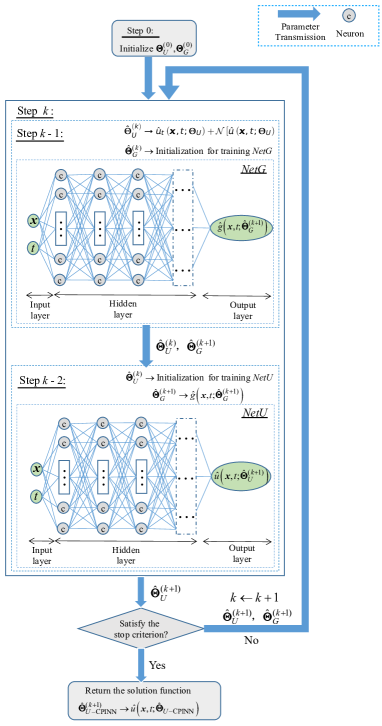
Figure 1: Architecture of CPINN.

III-D CPINN-RP for Soft Sensors

If PDEs include the partial derivative of temporal variables, the temporal dependence in the measurements can be used to improve the prediction performance. Note that the mean squared error loss function (9) can be considered a Monte-Carlo approximation of the second power of $L^{2}$-norm loss function (17). The training datasets are sampled with a fixed temporal interval. This discretization strategy can cause information loss. For this reason, CPINN is followed by RP to obtain CPINN-RP. In the first phase, CPINN composed of $NetU$ and $NetG$ is proposed to approximate PDEs solutions, and the hierarchical training strategy Algorithm 1 optimizes and couples the two networks to achieve parameter $\bm{\hat{\Theta}}_{U-\mathrm{C}\mathrm{PINN}}$. In the second phase, $NetU$ compensated with RP obtaining $NetU$-$RP$ to improve the prediction performance, which is initialized by $\bm{\hat{\Theta}}_{U}^{(k)}$. The spatial and temporal variables of CPINN inputs are still fed in $NetU$-$RP$. The rest inputs of $NetU$-$RP$ are fed in an either-or way: 1) If a hard sensor is available at a collocation point, its delayed measurements are used; 2) Otherwise, the delayed outputs of CPINN are used. The training strategy for $NetU$-$RP$ is shown in Fig. 2.

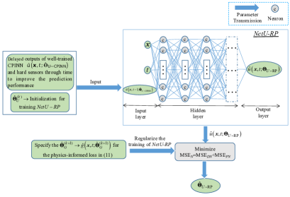
Figure 2: Training strategy for $NetU$-$RP$.

The same loss function for training CPINN is also used to train $NetU$-$RP$ to achieve the final CPINN-RP output $u\left(\bm{x},t;\bm{\hat{\Theta}}_{U-\mathrm{RP}}\right)$ as soft sensing results.

IV Numerical Experiments

In this section, the performance of CPINN-RP is verified with numerical experiments implemented with Pytorch. The fully-connected neural networks with hyperbolic tangent activation functions are used (ensuring Theorem 1 and Corollary 1 hold) and initialized by Xavier[37]. L-BFGS [38] is used to train CPINN-RP.

We evaluate the prediction performance of CPINN-RP by means of root mean squared error (RMSE)

$$\rm{RMSE}=\sqrt{\frac{1}{{\rm card}\left(T_{e}\right)}\sum_{(\bm{x},t,u)\in T_{e}}\left({\hat{u}\left(\bm{x},t\right)}-u\left(\bm{x},t\right)\right)^{2}},$$

where $T_{e}$ is the testing dataset. $\hat{u}\left(\bm{x},t\right)$ and $u\left(\bm{x},t\right)$ denote the prediction and the corresponding ground truth, respectively. To further validate the prediction performance of CPINN-RP, the Pearson correlation coefficient (CC)

$${\rm CC}=\frac{{\rm Cov}\left(\hat{u}\left(\bm{x},t\right),u\left(\bm{x},t\right)\right)}{\sqrt{{\rm Var}\left(\hat{u}\left(\bm{x},t\right)\right)}\sqrt{{\rm Var}\left(u\left(\bm{x},t\right)\right)}}$$

is also used to measure the similarity between prediction and ground truth, where ${\rm Cov}\left(\cdot,\cdot\right)$ is covariance and ${\rm Var}(\cdot)$ is variance.

IV-A Case 1: Heat Equation with Unmeasurable Heat Source Term

The heat equation was first developed for modeling how heat diffuses through a given region[39, 40]. CPINN-RP is first verified with the following heat equation

$$\left\{\begin{array}[]{ll}\displaystyle\frac{\partial u}{\partial t}=a^{2}\frac{\partial^{2}u}{\partial x^{2}}+g(x,t),\hskip 11.38109pt0<x<L,t>0\\[8.53581pt] \displaystyle\left.u\right|_{t=0}=\phi(x),\quad\hskip 39.83385pt0\leqslant x\leqslant L\\[5.69054pt] \displaystyle\left.u\right|_{x=0}=0,\left.\quad\frac{\partial u}{\partial x}\right|_{x=L}=0,\hskip 8.53581ptt>0\end{array},\right.$$ (24)

where the thermal diffusivity coefficient $a=1$, the length of the finite line $L=\pi$, the initial temperature $\phi(x)=\sin\left({x}/{2}\right)$, and the heat source $\displaystyle g(x)=\sin\left({x}/{2}\right)$. The exact solution $u(x,t)$ with respect to (24) is obtained according to [41]. The abovementioned setups are used to generate the training and testing datasets. Considering the practical situations, the heat source is assumed to be unmeasurable.

In this case, $NetU$ consists of 3 hidden layers of 30 neurons individually; $NetG$ is of 8 hidden layers of 20 neurons individually; $NetU$-$RP$ is of the same hidden layer structure as $NetU$. A total of 130 training data is randomly sampled from $D_{B}$. Moreover, the 20 sparse collocation points are randomly sampled to regularize the structure of (24). The abovementioned training dataset and the magnitude of predictions $\hat{u}(x,t)$ are shown in Fig. 3(a). Moreover, we compare the predictions and ground truths at fixed-time $t=3$ and 7 in Fig. 3(b) and (c), respectively. Table I shows the evaluation criteria for the prediction performance of CPINN-RP.

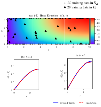
Figure 3: (a) Predictions $\hat{u}\left(x,t\right)$ for 1-D heat equation. (b) and (c) Comparisons of predictions and ground truths corresponding to fixed-time $t$=3 and 7 snapshots depicted by dashed vertical lines in (a), respectively.

TABLE I: Evaluation criteria for temporal snapshots are depicted by dashed vertical lines in Fig. 3-(a).

Criteria	3	7	$\left[0,\pi\right]\times\left[0,10\right]$
${\rm RMSE}$	1.633733e-02	3.920911e-02	4.234160e-02
CC	9.999875e-01	9.999571e-01	9.999368e-01

IV-B Case 2: Wave Equation with Unmeasurable Driving Force Term

The wave equation is a second-order linear PDE describing various fluctuation phenomena [42, 43]. In this section, we further verify CPINN-RP with the following wave equation

$$\left\{\begin{array}[]{ll}\displaystyle\frac{\partial^{2}u}{\partial t^{2}}=a^{2}\frac{\partial^{2}u}{\partial x^{2}}+g(x,t),\hskip 11.38109pt0<x<L,t>0\\[8.53581pt] \displaystyle\left.u\right|_{t=0}=0,\left.\quad\frac{\partial u}{\partial t}\right|_{t=0}=0,\hskip 11.38109pt0\leqslant x\leqslant L\\[8.53581pt] \displaystyle\left.u\right|_{x=0}=0,\left.\quad u\right|_{x=L}=0,\hskip 17.07164ptt>0\end{array},\right.$$ (25)

where the velocity $a=1$, the length of finite line $L=\pi$, the time of $t=6$, and the force $g(x,t)=\sin\frac{2\pi x}{L}\sin\frac{2a\pi t}{L}$. The acquisition of training and testing datasets is similar to Case 1.

In this experiment, $NetU$ consists of 3 hidden layers of 30 neurons individually; $NetG$ consists of 8 hidden layers of 20 units individually; $NetU$-$RP$ is of the same hidden layer structure as $NetU$. A total of 210 training data in $D$, 170 training data in $D_{B}$ and 40 training data in $D_{I}$, are randomly sampled. Fig. 4(a) shows the training dataset and the magnitude of predictions $\hat{u}(x,t)$. Fig. 4(b) and (c) show the comparisons of the predictions and ground truths corresponding to the fixed-time $t$ = 2 and 4. The prediction performance of CPINN-RP is further quantified in Table II.

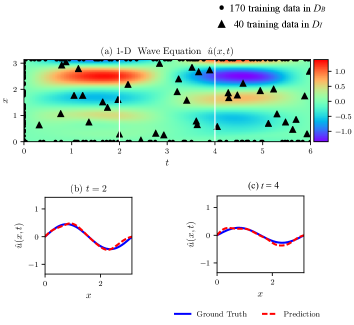
Figure 4: (a) Predictions $\hat{u}\left(x,t\right)$ for 1-D wave equation. (b) and (c) Comparisons of predictions and ground truths corresponding to fixed-time $t$=2 and 4 snapshots depicted by dashed vertical lines in (a), respectively.

TABLE II: Evaluation criteria for temporal snapshots are depicted by dashed vertical lines in Fig. 4-(a).

Criteria	2	4	$\left[0,\pi\right]\times\left[0,6\right]$
${\rm RMSE}$	4.844044e-02	5.280401e-02	6.748852e-02
CC	9.898351e-01	9.819893e-01	9.876968e-01

V Experimental Verification with Data from a Practical Vibration Process

In this section, the practical datasets sampled from aero-engine involute spline couplings fretting wear experiment platform are used to demonstrate the feasibility and effectiveness of CPINN-RP for soft sensors. The experiment system is presented in Fig. 5 and Fig. 6.

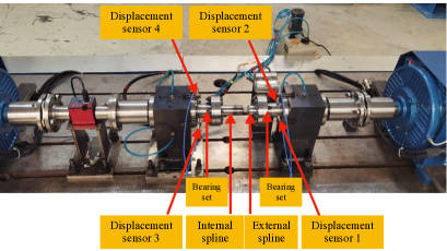
Figure 5: Aero-engine involute spline couplings fretting wear experiment platform.

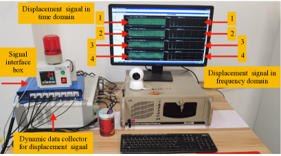
Figure 6: Data acquisition and processing system.

As shown in Fig. 5, the experiment platform is mainly composed of spline couplings, bearing sets, displacement sensors, and a motor drive. The data acquisition and processing system in Fig. 6 is used to monitor the vibration displacement of the internal and external spline shafts. The datasets are sampled with the condition as follows.

• The working speed of the motor drive is 3000 r/min.

• The sampling frequency is 2048Hz with 4096 sampling points.

The time-domain waveforms for the sampled signals are shown in Fig. 7.

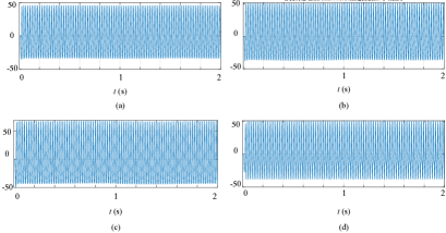
Figure 7: Raw displacement signals from sensors in time domain: (a) Sensor 1. (b) Sensor 2. (c) Sensor 3. (d) Sensor 4.

As described in Section iv@, the vibration displacement of the spline shaft is governed by (25). The distance $L$ between the shaft of two ends is $520$mm and measurements $u(x_{i},t)$ for $i=1,2,3,4$ are obtained from displacement sensors 1-4 as described in Fig. 5 and 6. The total number of training data is about 1$\%$ of the total sampled data. The measurements obtained from sensor 4 are assumed to be unavailable and CPINN-RP is used as a soft sensor for predicting the output of sensor 4. The setups of $NetU$, $NetG$, and $NetU$-$RP$ can be referred to Section iv@. The prediction performance of CPINN-RP is depicted in Table III.

TABLE III: Evaluation criteria for predictions in aero-engine involute spline couplings fretting wear experiment platform

Sensor	Criteria	Training	Testing	$\left[0,5.2\right]\times\left[0,2\right]$
1	RMSE	2.613778e-02	5.776048e+00	5.772521e+00
	CC	9.999967e-01	9.879768e-01	9.879771e-01
2	RMSE	1.088167e-02	5.449913e+00	5.446586e+00
	CC	9.999997e-01	9.909315e-01	9.909329e-01
3	RMSE	9.480886e-03	4.762897e+00	4.759989e+00
	CC	9.999998e-01	9.933763e-01	9.933794e-01
4	RMSE	2.144921e+00	8.222315e+00	8.217437e+00
	CC	9.997592e-01	9.714094e-01	9.714027e-01

Because the measurements of sensor 4 are unavailable, the soft sensing results for sensor 4 are not as good as the other three sensors, as shown in Table III. Although it does not outperform the hard sensors, CPINN-RP still offers feasible spatiotemporal predictions for difficult-to-measure variables and can be expected to as a core model for soft sensors.

VI Conclusion

This article proposed CPINN-RP for soft sensors. First, CPINN composed of $NetU$ and $NetG$ is proposed to approximate the solutions to nonhomogeneous PDEs. The proposed CPINN is theoretically proved to have a satisfying approximation capability for the solutions to the well-posed PDEs with unmeasurable source terms. Besides the theoretical aspects, $NetU$ and $NetG$ are optimized and coupled by the proposed hierarchical training strategy. Then, $NetU$-$RP$ is obtained with the recurrently delayed outputs of well-trained CPINN and hard sensors to further improve the prediction performance. Finally, the feasibility and effectiveness of CPINN-RP for soft sensors are validated with the artificial and practical datasets. Our method can be expected to benefit the soft sensors for industrial processes with spatiotemporal dependence and unmeasurable sources.

In the future, we will continue to use CPINN-RP as a soft sensor for more industrial scenarios other than the vibration processes. Meanwhile, more complex situations, such as PDEs with exactly unknown structures, will be considered in CPINN-RP. Feature extraction layers, such as convolution and pooling, will be added to CPINN-RP for architecture extensions.

References

- [1] C. F. Lui, Y. Liu, and M. Xie, “A supervised bidirectional long short-term memory network for data-driven dynamic soft sensor modeling,” IEEE Transactions on Instrumentation and Measurement, vol. 71, pp. 1–13, 2022.
- [2] K. Zhu and C. Zhao, “Dynamic graph-based adaptive learning for online industrial soft sensor with mutable spatial coupling relations,” IEEE Transactions on Industrial Electronics, vol. 70, no. 9, pp. 9614–9622, 2023.
- [3] X. Jiang and Z. Ge, “Improving the performance of just-in-time learning-based soft sensor through data augmentation,” IEEE Transactions on Industrial Electronics, vol. 69, no. 12, pp. 13 716–13 726, 2022.
- [4] G. Welch, G. Bishop et al., “An introduction to the kalman filter,” 1995.
- [5] F. Fischer and J. Deutscher, “Fault diagnosis for linear heterodirectional hyperbolic ode–pde systems using backstepping-based trajectory planning,” Automatica, vol. 135, p. 109952, 2022.
- [6] Y. Tang, H. Su, T. Jin, and R. C. Flesch, “Adaptive pid control approach considering simulated annealing algorithm for thermal damage of brain tumor during magnetic hyperthermia,” IEEE Transactions on Instrumentation and Measurement, 2023.
- [7] H. Karami, M. Azadifar, A. Mostajabi, P. Favrat, M. Rubinstein, and F. Rachidi, “Localization of electromagnetic interference sources using a time-reversal cavity,” IEEE Transactions on Industrial Electronics, vol. 68, no. 1, pp. 654–662, 2021.
- [8] J. Tu, C. Liu, and P. Qi, “Physics-informed neural network integrating pointnet-based adaptive refinement for investigating crack propagation in industrial applications,” IEEE Transactions on Industrial Informatics, pp. 1–9, 2022.
- [9] R. Pintelon, J. Schoukens, L. Pauwels, and E. Van Gheem, “Diffusion systems: stability, modeling, and identification,” IEEE Transactions on Instrumentation and Measurement, vol. 54, no. 5, pp. 2061–2067, 2005.
- [10] C. Oszkinat, S. E. Luczak, and I. Rosen, “Uncertainty quantification in estimating blood alcohol concentration from transdermal alcohol level with physics-informed neural networks,” IEEE Transactions on Neural Networks and Learning Systems, 2022.
- [11] J. Sirignano and K. Spiliopoulos, “Dgm: A deep learning algorithm for solving partial differential equations,” Journal of computational physics, vol. 375, pp. 1339–1364, 2018.
- [12] K. Kashinath, M. Mustafa, A. Albert, J. Wu, C. Jiang, S. Esmaeilzadeh, K. Azizzadenesheli, R. Wang, A. Chattopadhyay, A. Singh et al., “Physics-informed machine learning: case studies for weather and climate modelling,” Philosophical Transactions of the Royal Society A, vol. 379, no. 2194, p. 20200093, 2021.
- [13] X. Yuan, L. Li, Y. A. W. Shardt, Y. Wang, and C. Yang, “Deep learning with spatiotemporal attention-based lstm for industrial soft sensor model development,” IEEE Transactions on Industrial Electronics, vol. 68, no. 5, pp. 4404–4414, 2021.
- [14] X. Lu, T. Hu, and F. Yin, “A novel spatiotemporal fuzzy method for modeling of complex distributed parameter processes,” IEEE Transactions on Industrial Electronics, vol. 66, no. 10, pp. 7882–7892, 2019.
- [15] G. D. Smith, G. D. Smith, and G. D. S. Smith, Numerical solution of partial differential equations: finite difference methods. Oxford university press, 1985.
- [16] Z. Li, Z. Qiao, and T. Tang, Numerical solution of differential equations: introduction to finite difference and finite element methods. Cambridge University Press, 2017.
- [17] G. Dziuk and C. M. Elliott, “Finite element methods for surface pdes,” Acta Numerica, vol. 22, pp. 289–396, 2013.
- [18] J. Peiró and S. Sherwin, “Finite difference, finite element and finite volume methods for partial differential equations,” in Handbook of materials modeling. Springer, 2005, pp. 2415–2446.
- [19] J. N. Reddy, Introduction to the finite element method. McGraw-Hill Education, 2019.
- [20] X. Zhuang and C. Augarde, “Aspects of the use of orthogonal basis functions in the element-free galerkin method,” International Journal for Numerical Methods in Engineering, vol. 81, no. 3, pp. 366–380, 2010.
- [21] M. Ye, J. Shen, G. Lin, T. Xiang, L. Shao, and S. C. Hoi, “Deep learning for person re-identification: A survey and outlook,” IEEE transactions on pattern analysis and machine intelligence, vol. 44, no. 6, pp. 2872–2893, 2021.
- [22] R. Mondal, S. Bhowmik, and R. Sarkar, “tseggan: A generative adversarial network for segmenting touching nontext components from text ones in handwriting,” IEEE Transactions on Instrumentation and Measurement, vol. 70, pp. 1–10, 2021.
- [23] A. Kamble, P. H. Ghare, and V. Kumar, “Deep-learning-based bci for automatic imagined speech recognition using spwvd,” IEEE Transactions on Instrumentation and Measurement, vol. 72, pp. 1–10, 2023.
- [24] A. J. Meade Jr and A. A. Fernandez, “The numerical solution of linear ordinary differential equations by feedforward neural networks,” Mathematical and Computer Modelling, vol. 19, no. 12, pp. 1–25, 1994.
- [25] I. E. Lagaris, A. Likas, and D. I. Fotiadis, “Artificial neural networks for solving ordinary and partial differential equations,” IEEE transactions on neural networks, vol. 9, no. 5, pp. 987–1000, 1998.
- [26] I. E. Lagaris, A. C. Likas, and D. G. Papageorgiou, “Neural-network methods for boundary value problems with irregular boundaries,” IEEE Transactions on Neural Networks, vol. 11, no. 5, pp. 1041–1049, 2000.
- [27] M. Raissi, P. Perdikaris, and G. E. Karniadakis, “Physics-informed neural networks: A deep learning framework for solving forward and inverse problems involving nonlinear partial differential equations,” Journal of Computational physics, vol. 378, pp. 686–707, 2019.
- [28] M. Zhang, Q. Xu, and X. Wang, “Physics-informed neural network based online impedance identification of voltage source converters,” IEEE Transactions on Industrial Electronics, vol. 70, no. 4, pp. 3717–3728, 2023.
- [29] S. Cuomo, V. S. Di Cola, F. Giampaolo, G. Rozza, M. Raissi, and F. Piccialli, “Scientific machine learning through physics-informed neural networks: Where we are and what’s next,” arXiv preprint arXiv:2201.05624, 2022.
- [30] N. Zobeiry and K. D. Humfeld, “A physics-informed machine learning approach for solving heat transfer equation in advanced manufacturing and engineering applications,” Engineering Applications of Artificial Intelligence, vol. 101, p. 104232, 2021.
- [31] W. Chen, Q. Wang, J. S. Hesthaven, and C. Zhang, “Physics-informed machine learning for reduced-order modeling of nonlinear problems,” Journal of computational physics, vol. 446, p. 110666, 2021.
- [32] M. Yang and J. T. Foster, “Multi-output physics-informed neural networks for forward and inverse pde problems with uncertainties,” Computer Methods in Applied Mechanics and Engineering, p. 115041, 2022.
- [33] H. Gao, M. J. Zahr, and J.-X. Wang, “Physics-informed graph neural galerkin networks: A unified framework for solving pde-governed forward and inverse problems,” Computer Methods in Applied Mechanics and Engineering, vol. 390, p. 114502, 2022.
- [34] L. Guzzella and C. Onder, Introduction to modeling and control of internal combustion engine systems. Springer Science & Business Media, 2009.
- [35] S. Stenen Blakseth, A. Rasheed, T. Kvamsdal, and O. San, “Combining physics-based and data-driven techniques for reliable hybrid analysis and modeling using the corrective source term approach,” arXiv e-prints, pp. arXiv–2206, 2022.
- [36] A. G. Baydin, B. A. Pearlmutter, A. A. Radul, and J. M. Siskind, “Automatic differentiation in machine learning: a survey,” Journal of Marchine Learning Research, vol. 18, pp. 1–43, 2018.
- [37] Z. Fang, “A high-efficient hybrid physics-informed neural networks based on convolutional neural network,” IEEE Transactions on Neural Networks and Learning Systems, vol. 33, no. 10, pp. 5514–5526, 2021.
- [38] C. Zhu, R. H. Byrd, P. Lu, and J. Nocedal, “Algorithm 778: L-bfgs-b: Fortran subroutines for large-scale bound-constrained optimization,” ACM Transactions on mathematical software (TOMS), vol. 23, no. 4, pp. 550–560, 1997.
- [39] V. Bubanja, Y. Amagai, K. Okawa, and N.-H. Kaneko, “Mathematical modeling and measurement of low frequency characteristics of single-junction thermal converters,” IEEE Transactions on Instrumentation and Measurement, vol. 71, pp. 1–4, 2022.
- [40] B.-C. Wang, H.-X. Li, and H.-D. Yang, “Spatial correlation-based incremental learning for spatiotemporal modeling of battery thermal process,” IEEE Transactions on Industrial Electronics, vol. 67, no. 4, pp. 2885–2893, 2020.
- [41] B. R. Kusse and E. A. Westwig, Mathematical physics: applied mathematics for scientists and engineers. John Wiley & Sons, 2010.
- [42] Z. Liu, X. He, Z. Zhao, C. K. Ahn, and H.-X. Li, “Vibration control for spatial aerial refueling hoses with bounded actuators,” IEEE Transactions on Industrial Electronics, vol. 68, no. 5, pp. 4209–4217, 2021.
- [43] N. Chu, Y. Ning, L. Yu, Q. Liu, Q. Huang, D. Wu, and P. Hou, “Acoustic source localization in a reverberant environment based on sound field morphological component analysis and alternating direction method of multipliers,” IEEE Transactions on Instrumentation and Measurement, vol. 70, pp. 1–13, 2021.