Plane wave stability analysis of Hartree and quantum dissipative systems

Abstract

We investigate the stability of plane wave solutions of equations describing quantum particles interacting with a complex environment. The models take the form of PDE systems with a non local (in space or in space and time) self-consistent potential; such a coupling lead to challenging issues compared to the usual non linear Schrödinger equations. The analysis relies on the identification of suitable Hamiltonian structures and Lyapounov functionals. We point out analogies and differences between the original model, involving a coupling with a wave equation, and its asymptotic counterpart obtained in the large wave speed regime. In particular, while the analogies provide interesting intuitions, our analysis shows that it is illusory to obtain results on the former based on a perturbative analysis from the latter.

Keywords. Hartree equation. Open quantum systems. Particles interacting with a vibrational field. Schrödinger-Wave equation. Plane wave. Orbital stability.

Math. Subject Classification. 35Q40 35Q51 35Q55

1 Introduction

This work is concerned with the stability analysis of certain solutions of the following Hartree-type equation

$$\displaystyle i\partial_{t}U+\frac{1}{2}\Delta_{x}U=\gamma\left(\sigma_{1}\star_{x}\int_{\mathbb{R}^{n}}\sigma_{2}\Psi\,{\mathrm{d}}z\right)U,$$ (1a)

$$\displaystyle-\Delta_{z}\Psi=-\gamma\sigma_{2}(z)\left(\sigma_{1}\star_{x}|U|^{2}\right)(x)$$ (1b)

endowed with the initial condition

$$U\big{|}_{t=0}=U^{\mathrm{Init}},$$ (2)

and of the following Schrödinger-Wave system:

$$i\partial_{t}U+\displaystyle\frac{1}{2}\Delta_{x}U=\gamma\Phi U,$$ (3a)

$$\displaystyle\frac{1}{c^{2}}\partial_{tt}^{2}\Psi-\Delta_{z}\Psi=-\gamma\sigma_{2}(z)\sigma_{1}\star|U|^{2}(t,x),$$ (3b)

$$\Phi(t,x)=\displaystyle\iint_{\mathbb{T}^{d}\times\mathbb{R}^{n}}\sigma_{1}(x-y)\sigma_{2}(z)\Psi(t,y,z)\,{\mathrm{d}}z\,{\mathrm{d}}y,$$ (3c)

where $\gamma,c>0$ are given positive parameters, completed with

$$U\big{|}_{t=0}=U^{\mathrm{Init}},\qquad\Psi\big{|}_{t=0}=\Psi^{\mathrm{Init}},\qquad\partial_{t}\Psi\big{|}_{t=0}=\Pi^{\mathrm{Init}}.$$ (4)

The variable $x$ lies in the torus $\mathbb{T}^{d}$, meaning that the equations are understood with $(2\pi)-$periodicity in all directions. In 3b, the additional variable $z$ lies in $\mathbb{R}^{n}$ and, as explained below, it is crucial to assume $n\geq 3$. For reader’s convenience, the scaling of the equation is fully detailed in Appendix A; for our purposes the God-given form functions $\sigma_{1},\sigma_{2}$ are fixed once for all and the features of the coupling are embodied in the parameters $\gamma,c$. The system 1a-1b can be obtained, at least formally, from 3a-3c by letting the parameter $c$ run to $+\infty$, while $\gamma$ is kept fixed. By the way, system 1a-1b can be cast in the more usual form

$$i\partial_{t}U+\frac{1}{2}\Delta_{x}U=-\gamma^{2}\kappa\left(\Sigma\star_{x}|U|^{2}\right)U,\hskip 28.45274ptt\in\mathbb{R},\;x\in\mathbb{R}^{d}.$$ (5)

where

$$\kappa=\displaystyle\int_{\mathbb{R}^{n}}\sigma_{2}(z)(-\Delta_{z})^{-1}\sigma_{2}(z)\,{\mathrm{d}}z=\displaystyle\int_{\mathbb{R}^{n}}\displaystyle\frac{|\widehat{\sigma}_{2}(\xi)|^{2}}{|\xi|^{2}}\displaystyle\frac{\,{\mathrm{d}}\xi}{(2\uppi)^{n}}>0\text{ and }\Sigma=\sigma_{1}\star\sigma_{1}.$$ (6)

Letting now $\Sigma$ resemble the delta-Dirac mass, the asymptotic leads to the standard cubic non linear Schrödinger equation

$$i\partial_{t}U+\frac{1}{2}\Delta_{x}U=-\gamma^{2}\kappa|U|^{2}U.$$ (7)

in the focusing case. These asymptotic connections can be expected to shed some light on the dynamics of 3a-3c and to be helpful to guide the intuition about the behavior of the solutions, see [24, 25].

The motivation for investigating these systems takes its roots in the general landscape of the analysis of “open systems”, describing the dynamics of particles driven by momentum and energy exchanges with a complex environment. Such problems are modeled as Hamiltonian systems, and it is expected that the interaction mechanisms ultimately produce the dissipation of the particles’ energy, an idea which dates back to A. O. Caldeira and A. J. Leggett [7]. These issues have been investigated for various classical and quantum couplings, and with many different mathematical viewpoints, see e. g. [2, 3, 28, 29, 32, 33, 34]. The case in which the environment is described as a vibrational field, like in the definition of the potential by 3b-3c, is particularly appealing. In fact, 3a-3c is a quantum version of a model introduced by S. De Bièvre and L. Bruneau, dealing with a single classical particle [6]. Intuitively, the model of [6] can be thought of as if in each space position $x\in\mathbb{R}^{d}$ there is a membrane oscillating in a direction $z\in\mathbb{R}^{n}$, transverse to the motion of the particles. When a particle hits a membrane, its kinetic energy activates vibrations and the energy is evacuated at infinity in the $z-$direction. These energy transfer mechanisms eventually act as a sort of friction force on the particle, an intuition rigorously justified in [6, Theorem 2 and Theorem 4]. We refer the reader to [1, 13, 14, 34, 53] for further theoretical and numerical insight about this model. The model of [6] has been revisited by considering many interacting particles, which leads to Vlasov-type equations, still coupled to a wave equation for defining the potential [21]. Unexpectedly, asymptotic arguments indicate a connection with the attractive Vlasov-Poisson dynamic [12]. In turn, the particles-environment interaction can be interpreted in terms of Landau damping [22, 23]. The quantum version 3a-3c of the De Bièvre-Bruneau model has been discussed in [24, 25], with a connection to the kinetic model by means of a semi-classical analysis inspired from [39]. Note that in 3a-3c, the vibrational field remains of classical nature; a fully quantum framework is dealt with in [3, 15] for instance.

A remarkable feature of these systems is the presence of conserved quantities, here inherited from the framework designed in [6] for a classical particle, and the study of these models brings out the critical role of the wave speed $c>0$ and the dimension $n$ of the space for the wave equation (we can already notice that $n\geq 3$ is necessary for 6 to be meaningful), see [6, 22, 23, 25]. For the Schrödinger-Wave system 3a-3c the energy

$$H_{SW}(U,\Psi,\Pi)=\frac{1}{4}\int_{\mathbb{T}^{d}}|\nabla U|^{2}\,{\mathrm{d}}x+\iint_{\mathbb{T}^{d}\times\mathbb{R}^{n}}\left(\displaystyle{\color[rgb]{0,0,0}c^{2}}\Pi^{2}+{\color[rgb]{0,0,0}\frac{1}{4}}|\nabla_{z}\Psi|^{2}\right)\,{\mathrm{d}}x\,{\mathrm{d}}z+\frac{\gamma}{2}\int_{\mathbb{T}^{d}}\Phi|U|^{2}\,{\mathrm{d}}x,$$ (8)

is conserved since we can readily check that

$$\frac{\,{\mathrm{d}}}{\,{\mathrm{d}}t}H_{SW}(U,\Psi,{\color[rgb]{0,0,0}-\frac{1}{2c^{2}}}\partial_{t}\Psi)=0.$$

Similarly, for the Hartree system 1a-1b, we get

$$\frac{\,{\mathrm{d}}}{\,{\mathrm{d}}t}H_{Ha}(U)=0$$

where we have set

$$H_{Ha}(U)=\frac{1}{4}\int_{\mathbb{T}^{d}}|\nabla U|^{2}\,{\mathrm{d}}x-\gamma^{2}\frac{\kappa}{4}\int_{\mathbb{T}^{d}}\Sigma(x-y)|U(t,x)|^{2}|U(t,y)|^{2}\,{\mathrm{d}}y\,{\mathrm{d}}x.$$

Furthermore, for both model, the $L^{2}$ norm is conserved. Of course, these conservation properties play a central role for the analysis of the equations. However, 1a-1b has further fundamental properties which occur only for the asymptotic model: firstly, 1a-1b is Galilean invariant, which means that, given a solution $(t,x)\mapsto u(t,x)$ and for any $p_{0}\in\mathbb{T}^{d}$, the function $(t,x)\mapsto u(t,x-tp_{0})e^{i(x-tp_{0}/2)}$ is a solution too; secondly, the momentum $p(t)=\mathrm{Im}\int\bar{u}(t,x)\nabla_{x}u(t,x)\,{\mathrm{d}}x$ is conserved and, accordingly, the center of mass follows a straight line at constant speed. That these properties are not satisfied by the more complex system 3a-3c makes its analysis more challenging. Finally, we point out that, in contrast to the usual nonlinear Schrödinger equation or Hartree-Newton system, where $\Sigma$ is the Newtonian potential, the equations 1a-1b or 3a-3c do not fulfil a scale invariance property. This also leads to specific mathematical difficulties: despite the possible regularity of $\Sigma$, many results and approaches of the Newton case do not extend to a general kernel, due to the lack of scale invariance.

When the problem is set on the whole space $\mathbb{R}^{d}$, one is interested in the stability of solitary waves, which are solutions of the equation with the specific form $u(t,x)=e^{i\omega t}Q(x)$, and, for 3a-3c, $\psi(t,x,z)=\Psi(x,z)$. The details of the solitary wave are embodied into the Choquard equation, satisfied by the profile $Q$, [36, 40]. It turns out that the Choquard equation have infinitely many solutions; among these solutions, it is relevant to select the solitary wave which minimizes the energy functional under a mass constraint, [36, 41] and to study the orbital stability of this minimal energy state. This program has been investigated for 7 and 1a-1b in the specific case where $\Sigma(x)=\frac{1}{|x|}$ in dimension $d=3$, by various approaches [8, 35, 37, 38, 43, 56, 57]. Quite surprisingly, the specific form of the potential plays a critical role in the analysis (either through explicit formula or through scale invariance properties), and dealing with a general convolution kernel, as smooth as it is, leads to new difficulties, that can be treated by a perturbative argument, see [31, 58] for the case of the Yukawa potential, and [25] for 1a-1b and 3a-3c.

Here, we adopt a different viewpoint. We consider the case where the problem holds on the torus $\mathbb{T}^{d}$, and we are specifically interested in the stability of plane wave solutions of 3a-3c and 1a-1b. We refer the reader to [4, 5, 16, 44] for results on the nonlinear Schrödinger equation 7 in this framework. The discussion on the stability of these plane wave solutions will make the following smallness condition

$$4\gamma^{2}\kappa\|\sigma_{1}\|_{L^{1}}^{2}<1$$ (9)

(assuming the plane wave has an amplitude unity) appear. Despite its restriction to the periodic framework, the interest of this study is two-fold: on the one hand, it points out some difficulties specific to the coupling and provides useful hints for future works; on the other hand, it clarify the role of the parameters, by making stability conditions explicit.

The paper is organized as follows. In Section 2, we clarify the positioning of the paper. To this end, we further discuss some mathematical features of the model. We also introduce the main assumptions on the parameters that will be used throughout the paper and we provide an overview of the results. Section 3 is concerned with the stability analysis of the Hartree equation 1a-1b. Section 4 deals with the Schrödinger-Wave system at the price of restricting to the case where the wave vector of the plane wave solution vanishes: $k=0$. For reasons explained in details below, the general case is much more difficult. Section 5 justifies that in general the mode $k\neq 0$ is linearly and orbitally unstable. The proof splits into two steps. The former is concerned by the spectral instability; it relies on a suitable reformulation of the linearized operator, which allows us to count indirectly the eigenvalues. The latter step proves instability by using a contradiction argument and estimates established through the Duhamel formula. Finally, in Appendix A, we provide a physical interpretation of the parameters involved, and for the sake of completeness, in Appendices B and C, we discuss the well-posedness of the Schrödinger-Wave system 3a-3c and its link with the Hartree equation 1a-1b in the regime of large $c$’s.

2 Set up of the framework

2.1 Plane wave solutions and dispersion relation

For any $k\in\mathbb{Z}^{d}$, we start by seeking solutions to 3a-3c of the form

$$U(t,x)=U_{k}(t,x):=\exp\big{(}i(\omega t+k\cdot x)\big{)},\quad\Psi(t,x,z)=\Psi_{*}(z),\quad\partial_{t}\Psi(t,x,z)={\color[rgb]{0,0,0}-2c^{2}}\Pi_{*}(z)=0,$$ (10)

with $\omega\in\mathbb{R}$. Note that the $L^{2}$ norm of $U_{k}$ is $(2\uppi)^{d/2}$ and $\Psi_{*}$ actually does not depend on the time variable, nor on $x$. Since $|U_{k}(t,x)|=1$ is constant, the wave equation simplifies to

$${\frac{1}{c^{2}}}\partial_{tt}^{2}\Psi-\Delta_{z}\Psi=-\gamma\sigma_{2}(z)\big{\langle}{\sigma_{1}}\big{\rangle}_{\mathbb{T}^{d}},$$

where $\big{\langle}{\cdot}\big{\rangle}_{\mathbb{T}^{d}}$ stands for the average over $\mathbb{T}^{d}$: $\big{\langle}{f}\big{\rangle}_{\mathbb{T}^{d}}=\int_{\mathbb{T}^{d}}f(x)\,{\mathrm{d}}x$. As a consequence, $z\mapsto\Psi_{*}(z)$ is a solution to 3b if

$$\Psi_{*}(z)=-\gamma\Gamma(z)\big{\langle}{\sigma_{1}}\big{\rangle}_{\mathbb{T}^{d}},$$

with $\Gamma$ the solution of

$$-\Delta_{z}\Gamma(z)=\sigma_{2}(z).$$

This auxiliary function $\Gamma$ is thus defined by the convolution of $\sigma_{2}$ with the elementary solution of the Laplace operator in dimension $n$, or equivalently by means of Fourier transform:

$$\Gamma(z)=\int_{\mathbb{R}^{n}}\frac{C_{n}}{|z-z^{\prime}|^{n-2}}\sigma_{2}(z^{\prime})\,{\mathrm{d}}z^{\prime}=\mathscr{F}^{-1}_{\xi\to z}\Big{(}\displaystyle\frac{\widehat{\sigma}_{2}(\xi)}{|\xi|^{2}}\Big{)}.$$ (11)

The corresponding potential 3c is actually a constant which reads

$$-\gamma\displaystyle\iint_{\mathbb{T}^{d}\times\mathbb{R}^{n}}\sigma_{1}(x-y)\sigma_{2}(z)\Gamma(z)\big{\langle}{\sigma_{1}}\big{\rangle}_{\mathbb{T}^{d}}\,{\mathrm{d}}z\,{\mathrm{d}}y=-\kappa\gamma\big{\langle}{\sigma_{1}}\big{\rangle}_{\mathbb{T}^{d}}^{2}$$

with

$$\kappa=\displaystyle\int_{\mathbb{R}^{n}}\sigma_{2}(z)\Gamma(z)\,{\mathrm{d}}z=\displaystyle\int_{\mathbb{R}^{n}}|\nabla_{z}\Gamma(z)|^{2}\,{\mathrm{d}}z>0$$

(we remind the reader that this formula coincides with 6 and makes sense only when $n\geq 3$). It remains to identify the condition on the coefficients so that $U_{k}$ satisfies the Schrödinger equation 3a: this leads to the following dispersion relation

$$\omega+\frac{k^{2}}{2}-\Upsilon_{*}=0,\qquad\Upsilon_{*}=\gamma^{2}\kappa\big{\langle}{\sigma_{1}}\big{\rangle}_{\mathbb{T}^{d}}^{2}>0$$ (12)

with $k^{2}=\sum_{j=1}^{d}k_{j}^{2}$. We can compute explicitly the associated energy:

$$H_{SW}(U_{k},\Psi_{*},\Pi_{*})=\frac{(2\uppi)^{d}}{2}\left(\displaystyle\frac{k^{2}}{2}-\displaystyle\frac{\gamma^{2}\kappa}{2}\big{\langle}{\sigma_{1}}\big{\rangle}_{\mathbb{T}^{d}}^{2}\right)=\displaystyle\frac{(2\uppi)^{d}}{4}(k^{2}-\Upsilon_{*}).$$

Of course, among these solutions, the constant mode $U_{0}(t,x)=e^{i\omega t}{\mathbf{1}(x)}$ has minimal energy.

It turns out that the plane wave $U_{k}(t,x)=e^{i\omega t}e^{ik\cdot x}$ equally satisfies 1a-1b provided the dispersion relation 12 holds. Incidentally, we can check that

$$H_{Ha}(U_{k})=\frac{(2\uppi)^{d}}{2}\left(\displaystyle\frac{k^{2}}{2}-\displaystyle\frac{\gamma^{2}\kappa}{2}\big{\langle}{\Sigma}\big{\rangle}_{\mathbb{T}^{d}}\right)=\displaystyle\frac{(2\uppi)^{d}}{4}(k^{2}-\Upsilon_{*})$$

is made minimal when $k=0$.

2.2 Hamiltonian structure and symmetries of the problem

The conservation properties play a central role in the stability analysis, for instance in the reasonings that use concentration-compactness arguments [8]. Based on the conserved quantities, one can try to construct a Lyapounov functional, intended to evaluate how far a solution is from an equilibrium state. Then the stability analysis relies on the ability to prove a coercivity estimate on the variations of the Lyapounov functional, see [54, 56, 57]. This viewpoint can be further extended by identifying analogies with finite dimensional Hamiltonian systems with symmetries, which has permitted to set up a quite general framework [26, 27], revisited recently in [4]. The strategy relies on the ability in exhibiting a Hamiltonian formulation of the problem

$$\partial_{t}X=\mathbb{J}\partial_{X}\mathscr{H}(X),$$

where the symplectic structure is given by the skew-symmetric operator $\mathbb{J}$. As a consequence of Noether’s Theorem, this formulation encodes the conservation properties of the system. In particular, it implies that $t\mapsto\mathscr{H}(X(t))$ is a conserved quantity. For the problem under consideration, as it will be detailed below, $X$ is a vectorial unknown with components possibly depending on different variables ($x\in\mathbb{T}^{d}$ and $z\in\mathbb{R}^{n}$). This induces specific difficulties, in particular because the nature of the coupling is non local and delicate spectral issues arise related to the essential spectrum of the wave equation in $\mathbb{R}^{n}$. Next, we can easily observe that the systems 1a-1b and 3a-3c are invariant under multiplications by a phase factor of $U$, the “Schödinger unknown”, and under translations in the $x$ variable. This leads to the conservation of the $L^{2}$ norm of $U$ and of the total momentum. However, the systems 1a-1b and 3a-3c cannot be handled by a direct application of the results in [4, 26, 27]: the basic assumptions are simply not satisfied. Nevertheless, our approach is strongly inspired from [4, 26, 27]. As we will see later, for the Hartree system, a decisive advantage comes from the conservation of the total momentum and the Galilean invariance of the problem. For the Schrödinger-Wave problem, since the expression of the total momentum mixes up contribution from the “Schrödinger unknown” $U$ and the “wave unknown” $\Psi$, the information on its conservation does not seem readily useful.

In what follows, we find advantages in changing the unknown by writing $U(t,x)=e^{ik\cdot x}u(t,x)$; in turn the Schrödinger equation $i\partial_{t}U+\frac{1}{2}\Delta U=\Phi U$ becomes

$$i\partial_{t}u+\frac{1}{2}\Delta u-\frac{k^{2}}{2}u+ik\cdot\nabla u=\Phi u.$$

Accordingly, the parameter $k$ will appear in the definition the energy functional $\mathscr{H}$. This explains a major difference between 1a-1b and 3a-3c: for the former, a coercivity estimate can be obtained for the energy functional $\mathscr{H}$, for the latter, when $k\neq 0$ there are terms which cannot be controlled easily. This is reminiscent of the momentum conservation in 1a-1b and the lack of Galilean invariance for 3a-3c. The detailed analysis of the linearized operators sheds more light on the different behaviors of the systems 1a-1b and 3a-3c.

2.3 Outline of the main results

Let us collect the assumptions on the form functions $\sigma_{1}$ and $\sigma_{2}$ that govern the coupling:

• $\sigma_{1}:\mathbb{T}^{d}\rightarrow[0,\infty)$ is $C^{\infty}$ smooth, radially symmetric; $\big{\langle}{\sigma_{1}}\big{\rangle}_{\mathbb{T}^{d}}\neq 0$;

• $\sigma_{2}:\mathbb{R}^{n}\rightarrow[0,\infty)$ is $C^{\infty}$ smooth, radially symmetric and compactly supported;

• $(-\Delta)^{-1/2}\sigma_{2}\in L^{2}(\mathbb{R}^{n})$;

• for any $\xi\in\mathbb{R}^{n}$, $\widehat{\sigma}_{2}(\xi)\neq 0$.

Assumptions (H1)-(H2) are natural in the framework introduced in [6]. Hypothesis (H3) can equivalently be rephrased as $(-\Delta)^{-1}\sigma_{2}\in\accentset{\mbox{\large.}}{H}^{1}(\mathbb{R}^{n})$; it appears in many places of the analysis of such coupled systems and, at least, it makes the constant $\kappa$ in 6 meaningful. This constant is a component of the stability constraint 9. Hypothesis (H4) equally appeared in [6, Eq. (W)] when discussing large time asymptotic issues. Assumptions (H1)-(H4) are assumed throughout the paper.

Our results can be summarized as follows. We assume 9 and consider $k\in\mathbb{Z}^{d}$ and $\omega\in\mathbb{R}$ satisfying 12. For the Hartree equation, the analysis is quite complete:

• the plane wave $e^{i(\omega t+k\cdot x)}$ is spectrally stable (Theorem 3.1);

• for any initial perturbation with zero mean, the solutions of the linearized Hartree equation are $L^{2}$-bounded, uniformly over $t\geq 0$ (Theorem 3.3);

• the plane wave $e^{i(\omega t+k\cdot x)}$ is orbitally stable (Theorem 3.5).

For the Schrödinger-Wave system, the case $k=0$ is fully addressed as follows:

• the plane wave $(e^{i\omega t}\mathbf{1}(x),-\gamma\Gamma(z)\big{\langle}{\sigma_{1}}\big{\rangle}_{\mathbb{T}^{d}},0)$ is spectrally stable (Corollary 5.12);

• for any initial perturbation of $(e^{i\omega t}\mathbf{1}(x),-\gamma\Gamma(z)\big{\langle}{\sigma_{1}}\big{\rangle}_{\mathbb{T}^{d}},0)$ with zero mean, the solutions of the linearized Schrödinger-Wave system are $L^{2}$-bounded, uniformly over $t\geq 0$ (Theorem 4.2);

• the plane wave $(e^{i\omega t}\mathbf{1}(x),-\gamma\Gamma(z)\big{\langle}{\sigma_{1}}\big{\rangle}_{\mathbb{T}^{d}},0)$ is orbitally stable (Theorem 4.4).

When $k\neq 0$, the situation is much more involved; at least we prove that in general the plane wave solution $(e^{i(\omega t+k\cdot x)},-\gamma\Gamma(z)\big{\langle}{\sigma_{1}}\big{\rangle}_{\mathbb{T}^{d}},0)$ is spectrally unstable, see Section 5 and Corollary 5.15, and orbitally unstable, see Theorem 5.16.

Finally, let us mention that the approach presented here has been developed on an even simpler model, where the Schrödinger equation is replaced by a mere finite dimensional differential system [20].

3 Stability analysis of the Hartree system 1a-1b

To study the stability of the plane wave solutions of the Hartree system, it is useful to write the solutions of 1a-1b in the form

$$U(t,x)=e^{ik\cdot x}u(t,x)$$

with $u(t,x)$ solution to

$$i\partial_{t}u+\displaystyle\frac{1}{2}\Delta u-\displaystyle\frac{k^{2}}{2}u+ik\cdot\nabla u=-\gamma^{2}\kappa(\Sigma\star|u|^{2})u.$$ (13)

If $k\in\mathbb{Z}^{d}$ and $\omega\in\mathbb{R}$ satisfy the dispersion relation 12, $u_{\omega}(t,x)=e^{i\omega t}\mathbf{1}(x)$ is a solution to 13 with initial condition $u_{\omega}(0,t)=\mathbf{1}(x)$. Therefore, studying the stability properties of $U_{k}(t,x)=e^{i\omega t}e^{ik\cdot x}$ as a solution to 1a-1b amounts to studying the stability of $u_{\omega}(t,x)=e^{i\omega t}\mathbf{1}(x)$ as a solution to 13.

The problem 13 has an Hamiltonian symplectic structure when considered on the real Banach space $H^{1}(\mathbb{T}^{d};\mathbb{R})\times H^{1}(\mathbb{T}^{d};\mathbb{R})$. Indeed, if we write $u=q+ip$, with $p,q$ real-valued, we obtain

$$\partial_{t}\begin{pmatrix}q\\ p\end{pmatrix}=\mathbb{J}\nabla_{(q,p)}\mathscr{H}(q,p)$$

with

$$\mathbb{J}=\begin{pmatrix}0&1\\ -1&0\end{pmatrix}$$

and

$$\mathscr{H}(q,p)= \,\frac{1}{2}\left(\displaystyle\frac{1}{2}\displaystyle\int_{\mathbb{T}^{d}}|\nabla q|^{2}+|\nabla p|^{2}\,{\mathrm{d}}x+\frac{k^{2}}{2}\int_{\mathbb{T}^{d}}(p^{2}+q^{2})\,{\mathrm{d}}x-\int_{\mathbb{T}^{d}}pk\cdot\nabla q\,{\mathrm{d}}x+\int_{\mathbb{T}^{d}}qk\cdot\nabla p\,{\mathrm{d}}x\right)$$

$$-\frac{\gamma^{2}\kappa}{4}\displaystyle\int_{\mathbb{T}^{d}}\Sigma\star(p^{2}+q^{2})(p^{2}+q^{2})\,{\mathrm{d}}x.$$

Coming back to $u=q+ip$, we can write

$$\mathscr{H}(u)= \,\frac{1}{2}\left(\displaystyle\frac{1}{2}\displaystyle\int_{\mathbb{T}^{d}}|\nabla u|^{2}\,{\mathrm{d}}x+\frac{k^{2}}{2}\int_{\mathbb{T}^{d}}|u(x)|^{2}\,{\mathrm{d}}x+\int_{\mathbb{T}^{d}}k\cdot(-i\nabla u)\overline{u}\,{\mathrm{d}}x\right)$$

$$-\frac{\gamma^{2}\kappa}{4}\displaystyle\int_{\mathbb{T}^{d}}(\Sigma\star|u|^{2})(x)|u(x)|^{2}\,{\mathrm{d}}x.$$ (14)

As observed above, $\mathscr{H}$ is a constant of the motion.

Moreover, it is clear that 13 is invariant under multiplications by a phase factor so that $F(u)=\frac{1}{2}\|u\|^{2}_{L^{2}}$ is conserved by the dynamics. The quantities

$$G_{j}(u)=\frac{1}{2}\int_{\mathbb{T}^{d}}\left(\frac{1}{i}\partial_{x_{j}}u\right)\overline{u}\,{\mathrm{d}}x$$

are constants of the motion too, that correspond to the invariance under translations. Indeed, a direct verification leads to

$$\frac{\,{\mathrm{d}}}{\,{\mathrm{d}}t}G_{j}(u)(t)=\frac{\kappa\gamma^{2}}{2}\int_{\mathbb{T}^{d}}\int_{\mathbb{T}^{d}}\partial_{x_{j}}\Sigma(x-y)\star|u|^{2}(t,y)|u|^{2}(t,x)\,{\mathrm{d}}y\,{\mathrm{d}}x=0.$$

Finally, we shall endow the Banach space $H^{1}(\mathbb{T}^{d};\mathbb{R})\times H^{1}(\mathbb{T}^{d};\mathbb{R})$ with the inner product

$$\left\langle\begin{pmatrix}q\\ p\end{pmatrix}\Big{|}\begin{pmatrix}q^{\prime}\\ p^{\prime}\end{pmatrix}\right\rangle=\displaystyle\int_{\mathbb{T}^{d}}\big{(}pp^{\prime}+qq^{\prime})\,{\mathrm{d}}x.$$

that can be also interpreted as an inner product for complex-valued functions:

$$\langle u|u^{\prime}\rangle=\mathrm{Re}\displaystyle\int_{\mathbb{T}^{d}}u\overline{u^{\prime}}\,{\mathrm{d}}x.$$ (15)

3.1 Linearized problem and spectral stability

Let us expand the solution of 13 around $u_{\omega}$ as $u(t,x)=u_{\omega}(t,x)(1+w(t,x))$. The linearized equation for the fluctuation reads

$$i\partial_{t}w+\displaystyle\frac{1}{2}\Delta_{x}w+ik\cdot\nabla_{x}w=-2\gamma^{2}\kappa(\Sigma\star\mathrm{Re}(w)).$$ (16)

We split $w=q+ip$, $q=\mathrm{Re}(w)$, $p=\mathrm{Im}(w)$ so that 16 recasts as

$$\partial_{t}\begin{pmatrix}q\\ p\end{pmatrix}=\mathbb{L}_{k}\begin{pmatrix}q\\ p\end{pmatrix}$$ (17)

with the linear operator

$$\mathbb{L}_{k}:\begin{pmatrix}q\\ p\end{pmatrix}\longmapsto\begin{pmatrix}-k\cdot\nabla_{x}q-\displaystyle\frac{1}{2}\Delta_{x}p\\ \displaystyle\frac{1}{2}\Delta_{x}q+2\gamma^{2}\kappa\Sigma\star q-k\cdot\nabla_{x}p\end{pmatrix}.$$ (18)

From now on, while $(q,p)$ has been introduced as a pair of real-valued functions, we consider $\mathbb{L}_{k}$ as acting on the $\mathbb{C}$-vector space of complex-valued functions $L^{2}(\mathbb{T}^{d};\mathbb{C})\times L^{2}(\mathbb{T}^{d};\mathbb{C})$, and we study its spectrum.

Theorem 3.1 (Spectral stability for the Hartree equation)

Let $k\in\mathbb{Z}^{d}$ and $\omega\in\mathbb{R}$ such that the dispersion relation 12 is satisfied. Suppose 9 holds. Then the spectrum of $\mathbb{L}_{k}$, the linearization of 13 around the plane wave $u_{\omega}(t,x)=e^{i\omega t}\mathbf{1}(x)$, in $L^{2}(\mathbb{T}^{d};\mathbb{C})\times L^{2}(\mathbb{T}^{d};\mathbb{C})$ is contained in $i\mathbb{R}$. Consequently, this wave is spectrally stable in $L^{2}(\mathbb{T}^{d})$.

Proof. To prove Theorem 3.1, we expand $q$, $p$ and $\sigma_{1}$ by means of their Fourier series

$$\begin{array}[]{ll}q(t,x)=\displaystyle\sum_{m\in\mathbb{Z}^{d}}Q_{m}(t)e^{im\cdot x},&Q_{m}(t)=\displaystyle\frac{1}{(2\uppi)^{d}}\displaystyle\int_{\mathbb{T}^{d}}q(t,x)e^{-im\cdot x}\,{\mathrm{d}}x,\\[8.5359pt] p(t,x)=\displaystyle\sum_{m\in\mathbb{Z}^{d}}P_{m}(t)e^{im\cdot x},&P_{m}(t)=\displaystyle\frac{1}{(2\uppi)^{d}}\displaystyle\int_{\mathbb{T}^{d}}p(t,x)e^{-im\cdot x}\,{\mathrm{d}}x,\\ \sigma_{1}(x)=\displaystyle\sum_{m\in\mathbb{Z}^{d}}\sigma_{1,m}e^{im\cdot x},&\sigma_{1,m}(t)=\displaystyle\frac{1}{(2\uppi)^{d}}\displaystyle\int_{\mathbb{T}^{d}}\sigma_{1}(x)e^{-im\cdot x}\,{\mathrm{d}}x.\end{array}$$

Note that $\sigma_{1}$ being real and radially symmetric, we have

$$\overline{\sigma_{1,m}}=\sigma_{1,m}=\sigma_{1,-m}$$ (19)

and, by definition, $\big{\langle}{\sigma_{1}}\big{\rangle}_{\mathbb{T}^{d}}=(2\uppi)^{d}\sigma_{1,0}$. As a consequence, we obtain

$$\mathbb{L}_{k}\begin{pmatrix}q\\ p\end{pmatrix} =\begin{pmatrix}\sum_{m\in\mathbb{Z}^{d}}\left(\displaystyle\frac{m^{2}}{2}P_{m}-ik\cdot mQ_{m}\right)e^{im\cdot x}\\ \sum_{m\in\mathbb{Z}^{d}}\left(-\displaystyle\frac{m^{2}}{2}Q_{m}-ik\cdot mP_{m}+2(2\uppi)^{2d}\gamma^{2}\kappa|\sigma_{1,m}|^{2}Q_{m}\right)e^{im\cdot x}\end{pmatrix}$$

$$=\mathbb{L}_{k,0}\begin{pmatrix}Q_{0}\\ P_{0}\end{pmatrix}+\sum_{m\in\mathbb{Z}^{d}\smallsetminus\{0\}}\mathbb{L}_{k,m}\begin{pmatrix}Q_{m}\\ P_{m}\end{pmatrix}{\color[rgb]{0,0,0}e^{im\cdot x}}$$ (20)

with

$$\mathbb{L}_{k,0}=\begin{pmatrix}0&0\\ 2(2\uppi)^{2d}\gamma^{2}\kappa|\sigma_{1,0}|^{2}&0\end{pmatrix}\text{ and }\mathbb{L}_{k,m}=\begin{pmatrix}-ik\cdot m&\frac{m^{2}}{2}\\ -\frac{m^{2}}{2}+2(2\uppi)^{2d}\gamma^{2}\kappa|\sigma_{1,m}|^{2}&-ik\cdot m\end{pmatrix}$$ (21)

for $m\in\mathbb{Z}^{d}\smallsetminus\{0\}$.

Note that, since the Fourier modes are uncoupled, $\begin{pmatrix}q\\ p\end{pmatrix}$ is a solution to 17 if and only if the Fourier coefficients $\begin{pmatrix}Q_{m}\\ P_{m}\end{pmatrix}$ satisfy

$$\partial_{t}\begin{pmatrix}Q_{m}(t)\\ P_{m}(t)\end{pmatrix}=\mathbb{L}_{k,m}\begin{pmatrix}Q_{m}(t)\\ P_{m}(t)\end{pmatrix}$$

for any $m\in\mathbb{Z}^{d}$. Similarly, $\lambda\in\mathbb{C}$ is an eigenvalue of the operator $\mathbb{L}_{k}$ if and only if there exists at least one Fourier mode $m\in\mathbb{Z}^{d}$ such that $\lambda$ is an eigenvalue of the matrix $\mathbb{L}_{k,m}$, i.e. there exists $(q_{m},p_{m})\neq(0,0)$ such that

$$\begin{array}[]{l}\lambda q_{m}-\displaystyle\frac{m^{2}}{2}p_{m}+ik\cdot mq_{m}=0,\\[8.5359pt] \lambda p_{m}+\displaystyle\frac{m^{2}}{2}q_{m}+ik\cdot mp_{m}=2(2\uppi)^{2d}\gamma^{2}\kappa|\sigma_{1,m}|^{2}q_{m}.\end{array}$$ (22)

A straightforward computation gives that $\lambda_{0}=0$ is the unique eigenvalue of the matrix $\mathbb{L}_{k,0}$ with eigenvector $(0,1)$. This means that $\mathrm{Ker}(\mathbb{L}_{k})$ contains at least the vector subspace spanned by the constant function $x\in\mathbb{T}^{d}\mapsto\begin{pmatrix}0\\ 1\end{pmatrix}$, which corresponds to the constant solution $u(t,x)=i$ of 16.

Next, if $m\in\mathbb{Z}^{d}\smallsetminus\{0\}$, $\lambda_{m}$ is an eigenvalue of $\mathbb{L}_{k,m}$ if it is a solution to

$$(\lambda+ik\cdot m)^{2}-\frac{m^{2}}{2}\left(-\frac{m^{2}}{2}+2(2\uppi)^{2d}\gamma^{2}\kappa|\sigma_{1,m}|^{2}\right)=0.$$

This is a second order polynomial equation for $\lambda$ and the roots are given by

$$\lambda_{m,\pm}=-ik\cdot m\pm\displaystyle\frac{|m|}{2}\sqrt{-m^{2}+4\gamma^{2}\kappa(2\uppi)^{2d}|\sigma_{1,m}|^{2}}.$$

If the smallness condition 9 holds, the argument of the square root is negative for any $m\in\mathbb{Z}^{d}\smallsetminus\{0\}$, and thus the roots $\lambda$ are all purely imaginary (and we note that $\overline{\lambda_{-m,\pm}}=\lambda_{m,\mp}$). More precisely, we have the following statement.

Lemma 3.2 (Spectral stability for the Hartree equation)

Let $k,m\in\mathbb{Z}^{d}$ and $\mathbb{L}_{k,m}$ defined as in 21. Then

1. $\lambda_{0}=0$ is the unique eigenvalue of $\mathbb{L}_{k,0}$ and $\mathrm{Ker}(\mathbb{L}_{k,0})=\mathrm{span}\left\{\begin{pmatrix}0\\ 1\end{pmatrix}\right\}$;

2. for any $m\in\mathbb{Z}^{d}\smallsetminus\{0\}$, the eigenvalue of $\mathbb{L}_{k,m}$ are

   $$\lambda_{m,\pm}=-ik\cdot m\pm\displaystyle\frac{|m|}{2}\sqrt{-m^{2}+4\gamma^{2}\kappa(2\uppi)^{2d}|\sigma_{1,m}|^{2}}.$$

   1. if $4\gamma^{2}\kappa(2\uppi)^{2d}\frac{|\sigma_{1,m}|^{2}}{m^{2}}\leq 1$, then $\lambda_{m,\pm}\in i\mathbb{R}$;

   2. if $4\gamma^{2}\kappa(2\uppi)^{2d}\frac{|\sigma_{1,m}|^{2}}{m^{2}}>1$, then $\lambda_{m,\pm}\in\mathbb{C}\smallsetminus i\mathbb{R}$. Moreover, $\mathrm{Re}(\lambda_{m,+})>0$.

Now, 9 implies $4\gamma^{2}\kappa(2\uppi)^{2d}\frac{|\sigma_{1,m}|^{2}}{m^{2}}<1$ for all $m\in\mathbb{Z}^{d}\smallsetminus\{0\}$, so that $\sigma(\mathbb{L}_{k})\subset i\mathbb{R}$ and $u_{\omega}(t,x)=e^{i\omega t}\mathbf{1}(x)$ is spectrally stable. Conversely, if $\sigma_{1}$, $\sigma_{2}$ and $\gamma$ are such that there exists $m_{*}\in\mathbb{Z}^{d}\smallsetminus\{0\}$ verifying $4\gamma^{2}\kappa(2\uppi)^{2d}\frac{|\sigma_{1,m_{*}}|^{2}}{m_{*}^{2}}>1$, then the plane wave $u_{\omega}$ is spectrally unstable for any $k\in\mathbb{Z}^{d}$ and $\omega\in\mathbb{R}$ that satisfy the dispersion relation 12. This proves Theorem 3.1.  

We observe that this result is consistent with the linear stability analysis of 7, see [44, Theorem 1], when replacing formally $\Sigma$ by the delta-Dirac. The analogy should be considered with caution, though, since the functional difficulties are substantially different: here $u\mapsto-\frac{1}{2}\Delta_{\mathbb{T}^{d}}u-2\gamma^{2}\kappa\Sigma\star\mathrm{Re}(u)$ is a compact perturbation of $-\frac{1}{2}\Delta_{\mathbb{T}^{d}}$, which has a compact resolvent hence a spectral decomposition.

It is important to remark that the analysis of eigenproblems for $\mathbb{L}_{k}$ has consequences on the behavior of solutions to 17 of the particular form

$$Q(t,x)=e^{\lambda t}q(x),\qquad P(t,x)=e^{\lambda t}p(x).$$

We warn the reader that spectral stability excludes the exponential growth of the solutions of the linearized problem when the smallness condition 9 holds, but a slower growth is still possible. This can be seen by direct inspection for the mode $m=0$: we have $\partial_{t}Q_{0}=0$, so that $Q_{0}(t)=Q_{0}(0)$ and $\partial_{t}P_{0}=2(2\uppi)^{2d}\kappa\big{\langle}{\sigma_{1}}\big{\rangle}_{\mathbb{T}^{d}}^{2}Q_{0}(0)$ which shows that the solution can grow linearly in time

$$P_{0}(t)=P_{0}(0)+2(2\uppi)^{2d}\gamma^{2}\kappa\big{\langle}{\sigma_{1}}\big{\rangle}_{\mathbb{T}^{d}}^{2}Q_{0}(0)t.$$

In fact, excluding the mode $m=0$ suffices to guaranty the linearized stability.

Theorem 3.3 (Linearized stability for the Hartree equation)

Suppose 9. Let $w$ be the solution of 16 associated to an initial data $w^{\mathrm{Init}}\in H^{1}(\mathbb{T}^{d})$ such that $\int_{\mathbb{T}^{d}}w^{\mathrm{Init}}\,{\mathrm{d}}x=0$. Then, there exists a constant $C>0$ such that $\sup_{t\geq 0}\|w(t,\cdot)\|_{H^{1}}\leq C$.

Proof. Note that if $\int_{\mathbb{T}^{d}}w^{\mathrm{Init}}\,{\mathrm{d}}x=0$ then the corresponding Fourier coefficients $Q_{0}(0)$ and $P_{0}(0)$ are equal to $0$. As a consequence, $Q_{0}(t)=P_{0}(t)=0$ for all $t\geq 0$, so that $\int_{\mathbb{T}^{d}}w(t,x)\,{\mathrm{d}}x=0$ for all $t\geq 0$.

The proof follows from energetic consideration. Indeed, we observe that, on the one hand,

$$\begin{array}[]{l}\displaystyle\frac{1}{2}\displaystyle\frac{\,{\mathrm{d}}}{\,{\mathrm{d}}t}\displaystyle\int_{\mathbb{T}^{d}}|\nabla w|^{2}\,{\mathrm{d}}x=-\displaystyle\frac{\gamma^{2}\kappa}{2i}\displaystyle\int_{\mathbb{T}^{d}}\Sigma\star(w+\overline{w})\Delta(w-\overline{w})\,{\mathrm{d}}x,\end{array}$$

and, on the other hand,

$$\begin{array}[]{l}\displaystyle\frac{1}{2}\displaystyle\frac{\,{\mathrm{d}}}{\,{\mathrm{d}}t}\displaystyle\int_{\mathbb{T}^{d}}\Sigma\star(w+\overline{w})(w+\overline{w})\,{\mathrm{d}}x\\ \qquad=-\displaystyle\frac{1}{2i}\displaystyle\int_{\mathbb{T}^{d}}\Sigma\star(w+\overline{w})\Delta(w-\overline{w})\,{\mathrm{d}}x-k\cdot\displaystyle\int_{\mathbb{T}^{d}}\nabla(w+\overline{w})\Sigma\star(w+\overline{w})\,{\mathrm{d}}x,\end{array}$$

where we get rid of the last term in the right hand side by assuming $k=0$. This leads to the following energy conservation property

$$\frac{\,{\mathrm{d}}}{\,{\mathrm{d}}t}\left\{\displaystyle\frac{1}{2}\displaystyle\int_{\mathbb{T}^{d}}|\nabla w|^{2}\,{\mathrm{d}}x-\displaystyle\frac{\gamma^{2}\kappa}{2}\displaystyle\int_{\mathbb{T}^{d}}\Sigma\star(w+\overline{w})(w+\overline{w})\,{\mathrm{d}}x\right\}=0$$

which holds for $k=0$. We denote by $E_{0}$ the energy of the initial data $w^{\mathrm{Init}}$. Finally, we can simply estimate

$$\left|\displaystyle\int_{\mathbb{T}^{d}}\Sigma\star(w+\overline{w})(w+\overline{w})\,{\mathrm{d}}x\right|\leq\|\Sigma\star(w+\overline{w})\|_{L^{2}}\|w+\overline{w}\|_{L^{2}}\leq\|\Sigma\|_{L^{1}}\|w+\overline{w}\|^{2}_{L^{2}}\leq 4\|\Sigma\|_{L^{1}}\|w\|^{2}_{L^{2}}.$$

To conclude, we use the Poincaré-Wirtinger estimate. Indeed, since we have already remarked that the condition $\int_{\mathbb{T}^{d}}w^{\mathrm{Init}}\,{\mathrm{d}}x=0$ implies $\int_{\mathbb{T}^{d}}w(t,x)\,{\mathrm{d}}x=0$ for any $t\geq 0$, we can write

$$\left\|w(t,\cdot)\right\|_{L^{2}}^{2} =\Big{\|}w(t,\cdot)-\frac{1}{(2\uppi)^{d}}\displaystyle\int_{\mathbb{T}^{d}}w(t,y)\,{\mathrm{d}}y\Big{\|}^{2}_{L^{2}}=(2\uppi)^{d}\displaystyle\sum_{m\in\mathbb{Z}^{d}\smallsetminus\{0\}}|c_{m}(w(t,\cdot))|^{2}$$

$$\leq\displaystyle(2\uppi)^{d}\displaystyle\sum_{m\in\mathbb{Z}^{d}\smallsetminus\{0\}}m^{2}|c_{m}(w(t,\cdot))|^{2}=\|\nabla w(t,\cdot)\|^{2}_{L^{2}}$$

for any $t\geq 0$, where the $c_{m}(w(t,\cdot))$’s are the Fourier coefficients of the function $x\in\mathbb{T}^{d}\mapsto w(t,x)$. Hence, for any solution with zero mean, we infer, for all $t\geq 0$,

$$2E_{0}=\displaystyle\int_{\mathbb{T}^{d}}|\nabla w|^{2}(t,x)\,{\mathrm{d}}x-\displaystyle\gamma^{2}\kappa\displaystyle\int_{\mathbb{T}^{d}}\Sigma\star(w+\overline{w})(w+\overline{w})(t,x)\,{\mathrm{d}}x\geq(1-4\gamma^{2}\kappa\|\Sigma\|_{L^{1}})\int_{\mathbb{T}^{d}}|\nabla w(t,x)|^{2}\,{\mathrm{d}}x.$$

As a consequence, if 9 is satisfied, we obtain

$$\sup_{t\geq 0}\|w(t,\cdot)\|_{H^{1}}\leq 2\sqrt{\frac{E_{0}}{1-4\gamma^{2}\kappa\|\Sigma\|_{L^{1}}}}.$$

The stability estimate extends to the situation where $k\neq 0$. Indeed, from the solution $w$ of 16, we set

$$v(t,x)=w(t,x+tk).$$

It satisfies $i\partial_{t}v+\frac{1}{2}\Delta_{x}v=-2\gamma^{2}\kappa\Sigma\star\mathrm{Re}(v)$. Hence, repeating the previous argument, $\|v(t,\cdot)\|_{H^{1}}=\|w(t,\cdot)\|_{H^{1}}$ remains uniformly bounded on $(0,\infty)$. This step of the proof relies on the Galilean invariance of 5; it could have been used from the beginning, but it does not apply for the Schrödinger-Wave system.  

Remark 3.4

The analysis applies mutadis mutandis to any equation of the form 1a, with the potential defined by a kernel $\Sigma$ and a strength encoded by the constant $\gamma^{2}\kappa$. Then, the stability criterion is set on the quantity $4\gamma^{2}\kappa(2\uppi)^{d}\frac{|\widehat{\Sigma}_{m}|}{m^{2}}$ For instance, the elementary solution of $(a^{2}-\Delta_{x})\Sigma=\delta_{x=0}$ with periodic boundary condition has its Fourier coefficients given by $\widehat{\Sigma}_{m}=\frac{1}{(2\uppi)^{d}(a^{2}+m^{2})}>0$. Coming back to the physical variable, in the one-dimension case, the function $\Sigma$ reads

$$\Sigma(x)=\displaystyle\frac{e^{-a|x|}}{2a}+\displaystyle\frac{\cosh(ax)}{a(e^{2a\uppi}-1)}.$$

The linearized stability thus holds provided $4\gamma^{2}\kappa(2\uppi)^{2d}\frac{1}{a^{2}+1}<1$.

3.2 Orbital stability

In this subsection, we wish to establish the orbital stability of the plane wave $u_{\omega}(t,x)=e^{i\omega t}\mathbf{1}(x)$ as a solution to 13 for $k\in\mathbb{Z}^{d}$ and $\omega\in\mathbb{R}$ that satisfy the dispersion relation 12. As pointed out before, 13 is invariant under multiplications by a phase factor. This leads to define the corresponding orbit through $u(x)=\mathbf{1}(x)$ by

$$\mathscr{O}_{\mathbf{1}}=\{e^{i\theta},\ \theta\in\mathbb{R}\}.$$

Intuitively, orbital stability means that the solutions of 13 associated to initial data close enough to the constant function $x\in\mathbb{T}^{d}\mapsto 1=\mathbf{1}(x)$ remain at a close distance to the set $\mathscr{O}_{\mathbf{1}}$. Stability analysis then amounts to the construction of a suitable Lyapounov functional satisfying a coercivity property. This functional should be a constant of the motion and be invariant under the action of the group that generates the orbit $\mathscr{O}_{\mathbf{1}}$. Hence, the construction of such a functional relies on the invariants of the equation. Moreover, the plane wave has to be a critical point on the Lyapounov functional so that the coercivity can be deduced from the properties of its second variation. The difficulty here is that, in general, the bilinear symmetric form defining the second variation of the Lyapounov function is not positive on the whole space: according to the strategy designed in [26], see also the review [54], it will be enough to prove the coercivity on an appropriate subspace. Here and below, we adopt the framework presented in [4] (see also [5]).

Inspired by the strategy designed in [4, Section 8 & 9], we introduce, for any $k\in\mathbb{Z}^{d}$ and $\omega\in\mathbb{R}$ satisfying the dispersion relation 12, the set

$$\mathscr{S}_{\omega}=\Big{\{}u\in H^{1}(\mathbb{T}^{d};\mathbb{C}),\ F(u)=F(\mathbf{1})=\displaystyle\frac{(2\uppi)^{d}}{2}=(2\uppi)^{d}\displaystyle\frac{k^{2}/2+\omega}{2\gamma^{2}\kappa\big{\langle}{\sigma_{1}}\big{\rangle}_{\mathbb{T}^{d}}^{2}}\Big{\}};$$

$\mathscr{S}_{\omega}$ is therefore the level set of the solutions of 13, associated to the plane wave $(t,x)\mapsto u_{\omega}(t,x)=e^{i\omega t}\mathbf{1}(x)$. Next, we introduce the functional

$$\mathscr{L}_{\omega}(u)=\mathscr{H}(u)+\omega F(u)-\sum_{j=1}^{d}k_{j}G_{j}(u),$$ (23)

which is conserved by the solutions of 13. We have

$$\begin{array}[]{lll}\partial_{u}\mathscr{L}_{\omega}(u)(v)&=&\mathrm{Re}\left(\displaystyle\frac{1}{2}\displaystyle\int_{\mathbb{T}^{d}}(-\Delta u)\overline{v}\,{\mathrm{d}}x+\displaystyle\frac{k^{2}}{2}\displaystyle\int_{\mathbb{T}^{d}}u\overline{v}\,{\mathrm{d}}x\right.\\[8.5359pt] &&\left.\hskip 56.9055pt-\gamma^{2}\kappa\displaystyle\iint_{\mathbb{T}^{d}\times\mathbb{T}^{d}}\Sigma(x-y)|u(y)|^{2}u(x)\overline{v(x)}\,{\mathrm{d}}y\,{\mathrm{d}}x{+}\omega\displaystyle\int_{\mathbb{T}^{d}}u\overline{v}\,{\mathrm{d}}x\right).\end{array}$$

As a matter of fact, we observe that

$$\partial_{u}\mathscr{L}_{\omega}(\mathbf{1})=0$$

owing to the dispersion relation. Next, we get

$$\begin{array}[]{lll}\partial^{2}_{u}\mathscr{L}_{\omega}(u)(v,w)&=&\mathrm{Re}\left(\displaystyle\frac{1}{2}\displaystyle\int_{\mathbb{T}^{d}}(-\Delta+k^{2})w\overline{v}\,{\mathrm{d}}x\right.\\[8.5359pt] &&\left.-2\gamma^{2}\kappa\displaystyle\iint_{\mathbb{T}^{d}\times\mathbb{T}^{d}}\Sigma(x-y)\mathrm{Re}\big{(}\overline{u(y)}w(y)\big{)}u(x)\overline{v(x)}\,{\mathrm{d}}y\,{\mathrm{d}}x\right.\\[8.5359pt] &&\left.-\gamma^{2}\kappa\displaystyle\iint_{\mathbb{T}^{d}\times\mathbb{T}^{d}}\Sigma(x-y)|u(y)|^{2}w(x)\overline{v(x)}\,{\mathrm{d}}y\,{\mathrm{d}}x+\omega\displaystyle\int_{\mathbb{T}^{d}}w\overline{v}\,{\mathrm{d}}x\right).\end{array}$$

Still by using the dispersion relation, we obtain

$$\partial^{2}_{u}\mathscr{L}_{\omega}(\mathbf{1})(v,w)=\mathrm{Re}\left(\displaystyle\int_{\mathbb{T}^{d}}\underbrace{\left(-\displaystyle\frac{\Delta w}{2}-2\gamma^{2}\kappa\Sigma\star\mathrm{Re}(w)\right)}_{:=\mathbb{S}w}\overline{v(x)}\,{\mathrm{d}}x\right)=\langle\mathbb{S}w|v\rangle.$$

$\mathbb{S}:H^{2}(\mathbb{T}^{d})\subset L^{2}(\mathbb{T}^{d})\to L^{2}(\mathbb{T}^{d})$ is an unbounded linear operator and its spectral properties will play an important role for the orbital stability of $u_{\omega}$. Note that the operator $\mathbb{S}$ is the linearized operator 18, up to the advection term $k\cdot\nabla$. The main result of this subsection is the following.

Theorem 3.5 (Orbital stability for the Hartree equation)

Let $k\in\mathbb{Z}^{d}$ and $\omega\in\mathbb{R}$ such that the dispersion relation 12 is satisfied. Suppose 9 holds. Then the plane wave $u_{\omega}(t,x)=e^{i\omega t}\mathbf{1}(x)$ is orbitally stable, i.e.

$$\forall\varepsilon>0,\ \exists\delta>0,\ \forall v^{\mathrm{Init}}\in H^{1}(\mathbb{T}^{d};\mathbb{C}),\ \|v^{\mathrm{Init}}-\mathbf{1}\|_{H^{1}}<\delta\Rightarrow\sup_{t\geq 0}\mathrm{dist}(v(t),\mathscr{O}_{\mathbf{1}})<\varepsilon$$ (24)

where $\mathrm{dist}(v,\mathscr{O}_{\mathbf{1}})=\inf_{{\theta}\in[0,2\uppi[}\|v-e^{i{\theta}}\mathbf{1}\|_{H^{1}}$ and $(t,x)\mapsto v(t,x)\in C^{0}([0,\infty);H^{1}(\mathbb{T}^{d}))$ stands for the solution of 13 with Cauchy data $v^{\mathrm{Init}}$.

The full proof of Theorem 3.5 will be obtained from a series of intermediate steps, that we detail now. The key ingredient to prove Theorem 3.5 is the following coercivity estimate on the Lyapounov functional.

Lemma 3.6

Let $k\in\mathbb{Z}^{d}$ and $\omega\in\mathbb{R}$ such that the dispersion relation 12 is satisfied. Suppose that there exist $\eta>0$ and $c>0$ such that

$$\forall w\in\mathscr{S}_{\omega},d(w,\mathscr{O}_{\mathbf{1}})<\eta\Rightarrow\mathscr{L}_{\omega}(w)-\mathscr{L}_{\omega}(\mathbf{1})\geq c\ \mathrm{dist}(w,\mathscr{O}_{\mathbf{1}})^{2}.$$ (25)

Then the plane wave $u_{\omega}(t,x)=e^{i\omega t}\mathbf{1}(x)$ is orbitally stable.

Proof. Assume that 25 holds and suppose, by contradiction, that $u_{\omega}$ is not orbitally stable. Hence, there exists $0<\varepsilon_{0}<\frac{2}{3}\eta$ such that

$$\forall n\in{\mathbb{N}\smallsetminus\{0\},\ }\exists u_{n}^{\mathrm{Init}}\in H^{1}(\mathbb{T}^{d}),\|u_{n}^{\mathrm{Init}}-\mathbf{1}\|_{H^{1}}<\frac{1}{n}\text{ and }\exists t_{n}\in[0,+\infty[,\mathrm{dist}(u_{n}(t_{n}),\mathscr{O}_{\mathbf{1}})=\varepsilon_{0},$$

$(t,x)\mapsto u_{n}(t,x)\in C^{0}([0,\infty);H^{1}(\mathbb{T}^{d}))$ being the solution of 13 with Cauchy data $u_{n}^{\mathrm{Init}}$. To apply the coercivity estimate of Lemma 3.6, we define $z_{n}=\left(\frac{F(\mathbf{1})}{F(u_{n}(t_{n}))}\right)^{1/2}u_{n}(t_{n})$. It is clear that $z_{n}\in{\mathscr{S}_{\omega}}$ since $F(z_{n})=F(\mathbf{1})$. Moreover, $\big{(}u_{n}(t_{n})\big{)}_{n\in\mathbb{N}\smallsetminus\{0\}}$ is a bounded sequence in $H^{1}(\mathbb{T}^{d})$ and $\lim_{n\to+\infty}F(u_{n}(t_{n}))=F(\mathbf{1})$. Indeed, on the one hand, there exists $\gamma\in[0,2\uppi[$ such that

$$\|u_{n}(t_{n})\|_{H^{1}}\leq\|u_{n}(t_{n})-e^{i\theta}\mathbf{1}\|_{H^{1}}+\|e^{i\theta}\mathbf{1}\|_{H^{1}}\leq 2d(u_{n}(t_{n}),\mathscr{O}_{\mathbf{1}})+\|e^{i\theta}\mathbf{1}\|_{H^{1}}=2\varepsilon_{0}+\|\mathbf{1}\|_{H^{1}}$$

and, on the other hand,

$$|F(u_{n}(t_{n}))-F(\mathbf{1})|=\frac{1}{2}|\|u_{n}(t_{n})\|_{L^{2}}^{2}-\|\mathbf{1}\|^{2}_{L^{2}}|\leq\|u_{n}(t_{n})-\mathbf{1}\|_{L^{2}}(\varepsilon_{0}+\|\mathbf{1}\|_{H^{1}})<\frac{1}{n}(\varepsilon_{0}+\|\mathbf{1}\|_{H^{1}}).$$

As a consequence, $\lim_{n\to+\infty}\|z_{n}-u_{n}(t_{n})\|_{H^{1}}=0$. This implies for $n\in\mathbb{N}$ large enough,

$$\frac{\varepsilon_{0}}{2}\leq d(z_{n},\mathscr{O}_{\mathbf{1}})\leq\frac{3\varepsilon_{0}}{2}<\eta.$$

Hence, thanks to Lemma 3.6, we obtain

$$\mathscr{L}_{\omega}(u_{n}^{\mathrm{Init}})-\mathscr{L}_{\omega}(\mathbf{1}) =\mathscr{L}_{\omega}(u_{n}(t_{n}))-\mathscr{L}_{\omega}(\mathbf{1})=\mathscr{L}_{\omega}(u_{n}(t_{n}))-\mathscr{L}_{\omega}(z_{n})+\mathscr{L}_{\omega}(z_{n})-\mathscr{L}_{\omega}(\mathbf{1})$$

$$\geq\mathscr{L}_{\omega}(u_{n}(t_{n}))-\mathscr{L}_{\omega}(z_{n})+cd(z_{n},{\mathscr{O}_{\mathbf{1}}})^{2}\geq\mathscr{L}_{\omega}(u_{n}(t_{n}))-\mathscr{L}_{\omega}(z_{n})+\frac{c}{4}\varepsilon_{0}^{2}.$$

Finally, using the fact that $\partial_{u}\mathscr{L}_{\omega}(\mathbf{1})=0$ and $\partial_{u}^{2}\mathscr{L}_{\omega}(\mathbf{1})(w,w)\leq C\|w\|_{H^{1}}^{2}$, we deduce that

$$\lim_{n\to+\infty}(\mathscr{L}_{\omega}(u_{n}^{\mathrm{Init}})-\mathscr{L}_{\omega}(\mathbf{1}))=0,$$

$$\lim_{n\to+\infty}(\mathscr{L}_{\omega}(u_{n}(t_{n}))-\mathscr{L}_{\omega}(z_{n}))=0.$$

We are thus led to a contradiction.  

Since $\partial_{u}\mathscr{L}_{\omega}(\mathbf{1})=0$, the coercivity estimate 25 can be obtained from a similar estimate on the bilinear form $w\in H^{1}\mapsto\partial_{u}^{2}\mathscr{L}_{\omega}(\mathbf{1})(w,w)$. As pointed out before, the difficulty lies in the fact that, in general, this bilinear form is not positive on the whole space $H^{1}$. The following lemma states that it is enough to have a coercivity estimate on $\partial_{u}^{2}\mathscr{L}_{\omega}(\mathbf{1})(w,w)$ for any $w\in T_{\mathbf{1}}\mathscr{S}_{\omega}\cap(T_{\mathbf{1}}\mathscr{O}_{\mathbf{1}})^{\perp}$. Recall that the tangent set to $\mathscr{S}_{\omega}$ is given by

$$T_{\mathbf{1}}\mathscr{S}_{\omega}=\{u\in H^{1}(\mathbb{T}^{d};\mathbb{C}),\partial_{u}F(\mathbf{1})(u)=0\}=\left\{(q,p)\in H^{1}(\mathbb{T}^{d},\mathbb{R})\times H^{1}(\mathbb{T}^{d},\mathbb{R}),\ \Big{\langle}\begin{pmatrix}q\\ p\end{pmatrix}\Big{|}\begin{pmatrix}\mathbf{1}\\ {0}\end{pmatrix}\Big{\rangle}=0\right\}.$$

This set is the orthogonal to $\mathbf{1}$ with respect to the inner product defined in 15. The tangent set to $\mathscr{O}_{\mathbf{1}}$ (which is the orbit generated by the phase multiplication) is

$$T_{\mathbf{1}}\mathscr{O}_{\mathbf{1}}=\mathrm{span}_{\mathbb{R}}\{i\mathbf{1}\}$$

so that

$$(T_{\mathbf{1}}\mathscr{O}_{\mathbf{1}})^{\perp}=\{u\in H^{1}(\mathbb{T}^{d},\mathbb{C}),\langle u,i\mathbf{1}\rangle=0\}=\left\{(q,p):\mathbb{T}^{d}\to\mathbb{R},\ \Big{\langle}\begin{pmatrix}q\\ p\end{pmatrix}\Big{|}\begin{pmatrix}0\\ \mathbf{1}\end{pmatrix}\Big{\rangle}=0\right\}.$$

Lemma 3.7

Let $k\in\mathbb{Z}^{d}$ and $\omega\in\mathbb{R}$ such that the dispersion relation 12 is satisfied. Suppose that there exists $\tilde{c}>0$

$$\partial_{u}^{2}\mathscr{L}_{\omega}(\mathbf{1})(u,u)\geq\tilde{c}\|u\|^{2}_{H^{1}}$$ (26)

for any $u\in T_{\mathbf{1}}\mathscr{S}_{\mathbf{1}}\cap(T_{\mathbf{1}}\mathscr{O}_{\mathbf{1}})^{\perp}$. Then there exist $\eta>0$ and $c>0$ such that 25 is satisfied.

Proof. Let $w\in\mathscr{S}_{\omega}$ such that $\mathrm{dist}(w,\mathscr{O}_{\mathbf{1}})<\eta$ with $\eta>0$ small enough. By means of an implicit function theorem argument (see [4, Section 9, Lemma 8]), we obtain that there exists $\theta\in[0,2\uppi[$ and $v\in(T_{\mathbf{1}}\mathscr{O}_{\mathbf{1}})^{\perp}$ such that

$$e^{i{\theta}}w=\mathbf{1}+v,\qquad{\mathrm{dist}}(w,\mathscr{O}_{\mathbf{1}})\leq\|v\|_{H^{1}}\leq C{\mathrm{dist}}(w,\mathscr{O}_{\mathbf{1}})$$

for some positive constant $C$.

Next, we use the fact that $H^{1}(\mathbb{T}^{d})=T_{\mathbf{1}}\mathscr{S}_{\omega}\oplus\mathrm{span}_{\mathbb{R}}\{\mathbf{1}\}$ to write $v=v_{1}+v_{2}$ with $v_{1}\in T_{\mathbf{1}}\mathscr{S}_{\omega}\cap(T_{\mathbf{1}}\mathscr{O}_{\mathbf{1}})^{\perp}$ and $v_{2}\in\mathrm{span}_{\mathbb{R}}\{\mathbf{1}\}\cap(T_{\mathbf{1}}\mathscr{O}_{\mathbf{1}})^{\perp}$. Since $v=e^{i{\theta}}w-\mathbf{1}$ and $F(w)=F(\mathbf{1})$, we obtain

$$0=F(e^{i{\theta}}w)-F(\mathbf{1})=\frac{1}{2}\int_{\mathbb{T}^{d}}|v|^{2}\,{\mathrm{d}}x+\mathrm{Re}\int_{\mathbb{T}^{d}}(v_{1}+v_{2})\mathbf{1}\,{\mathrm{d}}x=\frac{1}{2}\int_{\mathbb{T}^{d}}|v|^{2}\,{\mathrm{d}}x+\mathrm{Re}\int_{\mathbb{T}^{d}}v_{2}\mathbf{1}\,{\mathrm{d}}x.$$

Since $v_{2}\in\mathrm{span}_{\mathbb{R}}\{\mathbf{1}\}$, it follows that

$$\|v_{2}\|_{H^{1}}\leq\frac{\|v\|_{H^{1}}^{2}}{{\color[rgb]{0,0,0}2}\|\mathbf{1}\|_{L^{2}}}.$$

This implies

$$\|v_{1}\|_{H^{1}}=\|v-v_{2}\|_{H^{1}}\geq\|v\|_{H^{1}}-{\color[rgb]{0,0,0}\frac{\|v\|_{H^{1}}^{2}}{2\|\mathbf{1}\|_{L^{2}}}}\geq\frac{1}{2}\|v\|_{H^{1}}$$

provided $\|v\|_{H^{1}}\leq\|\mathbf{1}\|_{L^{2}}$. As a consequence, if $\|v\|_{H^{1}}$ is small enough, using that $\partial_{u}^{2}\mathscr{L}_{\omega}(\mathbf{1})(w,z)\leq C\|w\|_{H^{1}}\|z\|_{H^{1}}$, we obtain

$$\partial_{u}^{2}\mathscr{L}_{\omega}(\mathbf{1})(v_{1},v_{2})\leq C\|v\|^{3}_{H^{1}},$$

$$\partial_{u}^{2}\mathscr{L}_{\omega}(\mathbf{1})(v_{2},v_{2})\leq C\|v\|^{4}_{H^{1}}.$$

This leads to

$$\partial_{u}^{2}\mathscr{L}_{\omega}(\mathbf{1})(v,v)=\partial_{u}^{2}\mathscr{L}_{\omega}(\mathbf{1})(v_{1},v_{1})+o(\|v\|^{2}_{H^{1}}).$$

Finally, let $w\in\mathscr{S}_{\omega}$ be such that $d(w,\mathscr{O}_{\mathbf{1}})<\eta$. We have

$$\mathscr{L}_{\omega}(w)-\mathscr{L}_{\omega}(\mathbf{1})=\mathscr{L}_{\omega}(e^{i{\theta}}w)-\mathscr{L}_{\omega}(\mathbf{1})=\frac{1}{2}\partial_{u}^{2}\mathscr{L}_{\omega}(\mathbf{1})(v,v)+o(\|v\|^{2}_{H^{1}})$$

$$=\frac{1}{2}\partial_{u}^{2}\mathscr{L}_{\omega}(\mathbf{1})(v_{1},v_{1})+o(\|v\|^{2}_{H^{1}})\geq{\color[rgb]{0,0,0}\displaystyle\frac{\tilde{c}}{2}}\|v_{1}\|^{2}_{H^{1}}+o(\|v\|^{2}_{H^{1}})\geq{\color[rgb]{0,0,0}\frac{\tilde{c}}{4}}\|v\|^{2}_{H^{1}}+o(\|v\|^{2}_{H^{1}})$$

$$\geq{\color[rgb]{0,0,0}\displaystyle\frac{\tilde{c}}{8}}{\mathrm{dist}}(w,\mathscr{O}_{\mathbf{1}})^{2}$$

where we use $\partial_{u}\mathscr{L}_{\omega}(\mathbf{1})=0$ and $v_{1}\in T_{\mathbf{1}}\mathscr{S}_{\omega}\cap(T_{\mathbf{1}}\mathscr{O}_{\mathbf{1}})^{\perp}$.  

At the end of the day, to prove the orbital stability of the plane wave $u_{\omega}(t,x)=e^{i\omega t}\mathbf{1}(x)$ it is enough to prove 26 for any $u\in T_{\mathbf{1}}\mathscr{S}_{\mathbf{1}}\cap(T_{\mathbf{1}}\mathscr{O}_{\mathbf{1}})^{\perp}$. This can be done by studying the spectral properties of the operator $\mathbb{S}$. However, in the simpler case of the Hartree equation, the coercivity of $\partial_{u}^{2}\mathscr{L}_{\omega}(\mathbf{1})$ on $T_{\mathbf{1}}\mathscr{S}_{\mathbf{1}}\cap(T_{\mathbf{1}}\mathscr{O}_{\mathbf{1}})^{\perp}$ can be also obtained directly from the expression

$$\partial^{2}_{u}\mathscr{L}_{\omega}(\mathbf{1})(u,u)=\mathrm{Re}\left(\displaystyle\int_{\mathbb{T}^{d}}\left(-\displaystyle\frac{\Delta u}{2}-2\gamma^{2}\kappa\Sigma\star\mathrm{Re}(u)\right)\overline{u(x)}\,{\mathrm{d}}x\right)=\langle\mathbb{S}u|u\rangle.$$ (27)

Let $u\in T_{\mathbf{1}}\mathscr{S}_{\mathbf{1}}\cap(T_{\mathbf{1}}\mathscr{O}_{\mathbf{1}})^{\perp}$ and write $u=q+ip$. This leads to

$$\partial^{2}_{u}\mathscr{L}_{\omega}(\mathbf{1})(u,u)=\frac{1}{2}\int_{\mathbb{T}^{d}}|\nabla q|^{2}\,{\mathrm{d}}x-2\gamma^{2}\kappa\int_{\mathbb{T}^{d}}(\Sigma\star q)q\,{\mathrm{d}}x+\frac{1}{2}\int_{\mathbb{T}^{d}}|\nabla p|^{2}\,{\mathrm{d}}x.$$

Moreover, since $u\in T_{\mathbf{1}}\mathscr{S}_{\mathbf{1}}\cap(T_{\mathbf{1}}\mathscr{O}_{\mathbf{1}})^{\perp}$, we have

$$\int_{\mathbb{T}^{d}}q\,{\mathrm{d}}x=0\text{ and }\int_{\mathbb{T}^{d}}p\,{\mathrm{d}}x=0.$$

As a consequence, thanks to the Poincaré-Wirtinger inequality, we deduce

$$\partial^{2}_{u}\mathscr{L}_{\omega}(\mathbf{1})(u,u)\geq\frac{1}{2}\int_{\mathbb{T}^{d}}|\nabla q|^{2}\,{\mathrm{d}}x-2\gamma^{2}\kappa\int_{\mathbb{T}^{d}}(\Sigma\star q)q\,{\mathrm{d}}x+\frac{1}{4}\|p\|^{2}_{H^{1}}.$$ (28)

Next, we expand $q$ and $\Sigma$ in Fourier series, i.e.

$$q(x)=\displaystyle\sum_{m\in\mathbb{Z}^{d}}q_{m}e^{im\cdot x}\text{ and }\Sigma(x)=\displaystyle\sum_{m\in\mathbb{Z}^{d}}\Sigma_{m}e^{im\cdot x}.$$

Note that, if $\Sigma=\sigma_{1}\star\sigma_{1}$, then $\Sigma_{m}=(2\uppi)^{d}\sigma_{1,m}^{2}$. Moreover, $\int_{\mathbb{T}^{d}}q\,{\mathrm{d}}x=0$ implies $q_{0}=0$. Hence,

$$\frac{1}{2}\int_{\mathbb{T}^{d}}|\nabla q|^{2}\,{\mathrm{d}}x-2\gamma^{2}\kappa\int_{\mathbb{T}^{d}}(\Sigma\star q)q\,{\mathrm{d}}x=(2\uppi)^{d}\sum_{m\in\mathbb{Z}^{d}\smallsetminus\{0\}}\left(\frac{m^{2}}{2}-2\gamma^{2}\kappa(2\uppi)^{d}\Sigma_{m}\right)q_{m}^{2}$$

$$=(2\uppi)^{d}\sum_{m\in\mathbb{Z}^{d}\smallsetminus\{0\}}\left(1-4\gamma^{2}\kappa(2\uppi)^{d}\frac{\Sigma_{m}}{m^{2}}\right)\frac{m^{2}}{2}q_{m}^{2}.$$ (29)

As a consequence, we obtain the following statement.

Proposition 3.8

Let $k\in\mathbb{Z}^{d}$ and $\omega\in\mathbb{R}$ such that the dispersion relation 12 is satisfied. Suppose that there exists $\delta\in(0,1)$ such that

$$4\gamma^{2}\kappa(2\uppi)^{2d}\frac{\sigma^{2}_{1,m}}{m^{2}}\leq\delta$$ (30)

for all $m\in\mathbb{Z}^{d}\smallsetminus\{0\}$. Then, there exists $\tilde{c}>0$ such that

$$\partial_{u}^{2}\mathscr{L}_{\omega}(\mathbf{1})(u,u)\geq\tilde{c}\|u\|^{2}_{H^{1}}$$ (31)

for any $u\in T_{\mathbf{1}}\mathscr{S}_{\mathbf{1}}\cap(T_{\mathbf{1}}\mathscr{O}_{\mathbf{1}})^{\perp}$.

Proof. If 30 holds, then 28-3.2 lead to

$$\partial^{2}_{u}\mathscr{L}_{\omega}(\mathbf{1})(u,u)\geq\frac{1-\delta}{2}(2\uppi)^{d}\sum_{m\in\mathbb{Z}^{d}\smallsetminus\{0\}}{m^{2}}q_{m}^{2}+\frac{1}{4}\|p\|_{H^{1}}=\frac{1-\delta}{2}\|\nabla q\|_{L^{2}}^{2}+\frac{1}{4}\|p\|^{2}_{H^{1}}\geq\frac{1-\delta}{4}\|u\|_{H^{1}}^{2}.$$

where in the last inequality we used the Poincaré-Wirtinger inequality together with the fact that $\int_{\mathbb{T}^{d}}q\,{\mathrm{d}}x=0$.  

Remark 3.9

By decomposing the linear operator $\mathbb{S}$ into real and imaginary part and by using Fourier series, one can study its spectrum. In particular, $\mathbb{S}$ has exactly one negative eigenvalue $\lambda_{-}=-2\gamma^{2}\kappa\big{\langle}{\Sigma}\big{\rangle}_{\mathbb{T}^{d}}$ with eigenspace $\mathrm{span}_{\mathbb{R}}\{\mathbf{1}\}$. Moreover, $\mathrm{Ker}(\mathbb{S})=\mathrm{span}_{\mathbb{R}}\{i\mathbf{1}\}$. Finally, if 30 is satisifed, then $\inf(\sigma(\mathbb{S})\cap(0,\infty))\geq\frac{1-\delta}{2}$. Then, by applying the same arguments as in [5, Section 6], we can recover the coercivity of $\partial_{u}^{2}\mathscr{L}_{\omega}(\mathbf{1})$ on $T_{\mathbf{1}}\mathscr{S}_{\mathbf{1}}\cap(T_{\mathbf{1}}\mathscr{O}_{\mathbf{1}})^{\perp}$.

Finally, Proposition 3.8 together with Lemma 3.7 and Lemma 3.6, gives Theorem 3.5 and the orbital stability of the plane wave $u_{\omega}$.

4 Stability analysis of the Schrödinger-Wave system: the case $k=0$

Like in the case of the Hartree system, to study the stability of the plane wave solutions of the Schrödinger-Wave system 3a-3c, it is useful to write its solutions in the form

$$U(t,x)=e^{ik\cdot x}u(t,x)$$

with $(t,x,z)\mapsto(u(t,x),\Psi(t,x,z))$ solution to

$$i\partial_{t}u+\frac{1}{2}\Delta_{x}u-\frac{k^{2}}{2}u+ik\cdot\nabla_{x}u=\left(\gamma\sigma_{1}\star\int_{\mathbb{R}^{n}}\sigma_{2}\Psi\,{\mathrm{d}}z\right)u,$$ (32)

$$\frac{1}{c^{2}}\partial^{2}_{tt}\Psi-\Delta_{z}\Psi=-\gamma\sigma_{2}\sigma_{1}\star|u|^{2}.$$

If $k\in\mathbb{Z}^{d}$ and $\omega\in\mathbb{R}$ satisfy the dispersion relation 12,

$$u_{\omega}(t,x)=e^{i\omega t}\mathbf{1}(x),\quad\Psi_{*}(t,x,z)=-\gamma\Gamma(z)\big{\langle}{\sigma_{1}}\big{\rangle}_{\mathbb{T}^{d}},\quad\Pi_{*}(t,x,z)={\color[rgb]{0,0,0}-\frac{1}{2c^{2}}}\partial_{t}\Psi_{*}(t,x,z)=0$$

with $\Gamma$ the solution of $-\Delta_{z}\Gamma=\sigma_{2}$ (see 11), is a solution to 32 with initial condition

$$u_{\omega}(0,{\color[rgb]{0,0,0}x})=\mathbf{1}(x),\quad\Psi_{*}(0,x,z)=-\gamma\Gamma(z)\big{\langle}{\sigma_{1}}\big{\rangle}_{\mathbb{T}^{d}},\quad\Pi_{*}(0,x,z)=0.$$

For the time being, we stick to the framework identified for the study of the asymptotic Hartree equation. Problem 32 has a natural Hamiltonian symplectic structure when considered on the real Banach space $H^{1}(\mathbb{T}^{d})\times H^{1}(\mathbb{T}^{d})\times L^{2}(\mathbb{T}^{d};\accentset{\mbox{\large.}}{H}^{1}(\mathbb{R}^{n}))\times L^{2}(\mathbb{T}^{d}\times\mathbb{R}^{n})$. Indeed, if we write $u=q+ip$, with $p,q$ real-valued, we obtain

$$\partial_{t}\begin{pmatrix}q\\ p\\ \Psi\\ \Pi\end{pmatrix}=\begin{pmatrix}\mathbb{J}&0\\ 0&-\mathbb{J}\end{pmatrix}\nabla_{(q,p,\Psi,\Pi)}\mathscr{H}_{SW}(q,p,\Psi,\Pi)$$

with

$$\mathbb{J}=\begin{pmatrix}0&1\\ -1&0\end{pmatrix}$$

and

$$\mathscr{H}_{SW}(q,p,\Psi,\Pi)= \,\frac{1}{2}\left(\displaystyle\frac{1}{2}\displaystyle\int_{\mathbb{T}^{d}}|\nabla q|^{2}+|\nabla p|^{2}\,{\mathrm{d}}x+\frac{k^{2}}{2}\int_{\mathbb{T}^{d}}(p^{2}+q^{2})\,{\mathrm{d}}x-\int_{\mathbb{T}^{d}}pk\cdot\nabla q\,{\mathrm{d}}x+\int_{\mathbb{T}^{d}}qk\cdot\nabla p\,{\mathrm{d}}x\right)$$

$$+\int_{\mathbb{T}^{d}\times\mathbb{R}^{n}}\left({\color[rgb]{0,0,0}c^{2}}\Pi^{2}+{\color[rgb]{0,0,0}\frac{1}{4}}|\nabla_{z}\Psi|^{2}\right)\,{\mathrm{d}}x\,{\mathrm{d}}z$$

$$+\frac{\gamma}{2}\displaystyle\int_{\mathbb{T}^{d}}\left(\int_{\mathbb{T}^{d}\times\mathbb{R}^{n}}(\sigma_{1}(x-y)\sigma_{2}(z)\Psi(t,y,z)\,{\mathrm{d}}y\,{\mathrm{d}}z\right)(p^{2}+q^{2})(x)\,{\mathrm{d}}x.$$

Coming back to $u=q+ip$, we can write

$$\mathscr{H}_{SW}(u,\Psi,\Pi)= \,\frac{1}{2}\left(\displaystyle\frac{1}{2}\displaystyle\int_{\mathbb{T}^{d}}|\nabla u|^{2}\,{\mathrm{d}}x+\frac{k^{2}}{2}\int_{\mathbb{T}^{d}}|u(x)|^{2}\,{\mathrm{d}}x+\int_{\mathbb{T}^{d}}k\cdot(-i\nabla u)\overline{u}\,{\mathrm{d}}x\right)$$

$$+\int_{\mathbb{T}^{d}\times\mathbb{R}^{n}}\left({\color[rgb]{0,0,0}c^{2}}\Pi^{2}+{\color[rgb]{0,0,0}\frac{1}{4}}|\nabla_{z}\Psi|^{2}\right)\,{\mathrm{d}}x\,{\mathrm{d}}z$$

$$+\frac{\gamma}{2}\displaystyle\int_{\mathbb{T}^{d}}\left(\int_{\mathbb{T}^{d}\times\mathbb{R}^{n}}(\sigma_{1}(x-y)\sigma_{2}(z)\Psi(t,y,z)\,{\mathrm{d}}y\,{\mathrm{d}}z\right)|u(x)|^{2}\,{\mathrm{d}}x.$$ (33)

As a consequence, $\mathscr{H}_{SW}$ is a constant of the motion. Moreover, it is clear that 32 is invariant under multiplications by a phase factor of $u$ so that $F(u)=\frac{1}{2}\|u\|^{2}_{L^{2}}$ is conserved by the dynamics. However, now, the quantities

$$G_{j}(u)=\frac{1}{2}\int_{\mathbb{T}^{d}}\left(\frac{1}{i}\partial_{x_{j}}u\right)\overline{u}\,{\mathrm{d}}x$$ (34)

are not constants of the motion:

$$\frac{\,{\mathrm{d}}}{\,{\mathrm{d}}t}G_{j}(u)(t)=\frac{\gamma}{2}\int_{\mathbb{T}^{d}}\int_{\mathbb{T}^{d}}\partial_{x_{j}}\sigma_{1}(x-y)\left(\int_{\mathbb{R}^{n}}\sigma_{2}(z)\Psi(t,y,z)\,{\mathrm{d}}z\right)|u|^{2}(t,x)\,{\mathrm{d}}y\,{\mathrm{d}}x.$$

As a consequence, they cannot be used in the construction of the Lyapounov functional as we did for the Hartree system (see 23).

Finally, we consider the Banach space $H^{1}(\mathbb{T}^{d})\times H^{1}(\mathbb{T}^{d})\times L^{2}(\mathbb{T}^{d};\accentset{\mbox{\large.}}{H}^{1}(\mathbb{R}^{n}))\times L^{2}(\mathbb{T}^{d}\times\mathbb{R}^{n})$ endowed with the inner product

$$\left\langle\begin{pmatrix}q\\ p\\ \Psi\\ \Pi\end{pmatrix}\Big{|}\begin{pmatrix}q^{\prime}\\ p^{\prime}\\ \Psi^{\prime}\\ \Pi^{\prime}\end{pmatrix}\right\rangle=\displaystyle\int_{\mathbb{T}^{d}}\big{(}pp^{\prime}+qq^{\prime})\,{\mathrm{d}}x+\int_{\mathbb{T}^{d}\times\mathbb{R}^{n}}(\nabla_{z}\Psi\nabla_{z}\Psi^{\prime}+\Pi\Pi^{\prime})\,{\mathrm{d}}x\,{\mathrm{d}}z$$

that can be also interpreted as an inner product for complex valued functions:

$$\langle(u,\Psi,\Pi)|(u^{\prime},\Psi^{\prime},\Pi^{\prime})\rangle=\mathrm{Re}\displaystyle\int_{\mathbb{T}^{d}}u\overline{u^{\prime}}\,{\mathrm{d}}x+\int_{\mathbb{T}^{d}\times\mathbb{R}^{n}}(\nabla_{z}\Psi\cdot\nabla_{z}\Psi^{\prime}+\Pi\Pi^{\prime})\,{\mathrm{d}}x\,{\mathrm{d}}z.$$ (35)

We denote by $\|\cdot\|$ the norm on $H^{1}(\mathbb{T}^{d})\times L^{2}(\mathbb{T}^{d};\accentset{\mbox{\large.}}{H}^{1}(\mathbb{R}^{n}))\times L^{2}(\mathbb{T}^{d}\times\mathbb{R}^{n})$ induced by this inner product.

4.1 Preliminary results for the linearized problem: spectral stability when $k=0$

As before, we linearize the system 3a-3c around the plane wave solution obtained in Section 2.1. Namely, we expand

$$U(t,x)=U_{k}(t,x)(\mathbf{1}+u(t,x)),\qquad\Psi(t,x,z)=-\gamma\big{\langle}{\sigma_{1}}\big{\rangle}_{\mathbb{T}^{d}}\Gamma(z)+\psi(t,x,z)$$

and, assuming that $u,\psi$ and their derivatives are small, we are led to the following equations for the fluctuation $(t,x)\mapsto u(t,x)\in\mathbb{C}$, $(t,x,z)\mapsto\psi(t,x,z)\in\mathbb{R}$

$$\begin{array}[]{l}i\partial_{t}u+\displaystyle\frac{1}{2}\Delta_{x}u+ik\cdot\nabla_{x}u=\gamma\Phi,\\[8.5359pt] \Big{(}\displaystyle\frac{1}{c^{2}}\partial_{tt}^{2}\psi-\Delta_{z}\psi\Big{)}(t,x,z)=-\gamma\par\sigma_{2}(z)\sigma_{1}\star\rho(t,x),\\[8.5359pt] \rho(t,x)=2\mathrm{Re}\big{(}u(t,x)\big{)},\\[8.5359pt] \Phi(t,x)=\displaystyle\iint_{\mathbb{T}^{d}\times\mathbb{R}^{n}}\sigma_{1}(x-y)\sigma_{2}(z)\psi(t,y,z)\,{\mathrm{d}}z\,{\mathrm{d}}y.\end{array}$$ (36)

We split the solution into real and imaginary parts

$$u(t,x)=q(t,x)+ip(t,x),\qquad q(t,x)=\mathrm{Re}(u(t,x)),\qquad p(t,x)=\mathrm{Im}(u(t,x)).$$

We obtain

$$\begin{array}[]{l}(\partial_{t}q+\displaystyle\frac{1}{2}\Delta_{x}p+k\cdot\nabla_{x}q)(t,x)=0,\\[8.5359pt] (\partial_{t}p-\displaystyle\frac{1}{2}\Delta_{x}q+k\cdot\nabla_{x}p)(t,x)=-\gamma\left(\sigma_{1}\star\displaystyle\int_{\mathbb{R}^{n}}\sigma_{2}(z)\psi(t,\cdot,z)\,{\mathrm{d}}z\right)(x),\\[8.5359pt] \Big{(}\displaystyle\frac{1}{c^{2}}\partial_{tt}^{2}\psi-\Delta_{z}\psi\Big{)}(t,x,z)=-2\gamma\sigma_{2}(z)\sigma_{1}\star q(t,x).\end{array}$$ (37)

It is convenient to set

$$\pi=-\frac{1}{2c^{2}}\partial_{t}\psi,$$

in order to rewrite the wave equation as a first order system. We obtain

$$\partial_{t}\begin{pmatrix}q\\ p\\ \psi\\ \pi\end{pmatrix}=\mathbb{L}_{k}\begin{pmatrix}q\\ p\\ \psi\\ \pi\end{pmatrix}$$ (38)

where $\mathbb{L}_{k}$ is the operator defined by

$$\mathbb{L}_{k}:\begin{pmatrix}q\\ p\\ \psi\\ \pi\end{pmatrix}\longmapsto\begin{pmatrix}-\displaystyle\dfrac{1}{2}\Delta_{x}p-k\cdot\nabla_{x}q\\ \displaystyle\frac{1}{2}\Delta_{x}q-k\cdot\nabla_{x}p-\gamma\sigma_{1}\star\left(\displaystyle\int_{\mathbb{R}^{n}}\sigma_{2}\psi\,{\mathrm{d}}z\right)\\ -2c^{2}\pi\\ -\displaystyle\frac{1}{2}\Delta_{z}\psi+\gamma\sigma_{2}\sigma_{1}\star q\end{pmatrix}.$$

For the next step, we proceed via Fourier analysis as before. We expand $q$, $p$, $\psi$, $\pi$ and $\sigma_{1}$ by means of their Fourier series:

$$\begin{array}[]{ll}\psi(t,x,z)=\displaystyle\sum_{m\in\mathbb{Z}^{d}}\psi_{m}(t,z)e^{im\cdot x},&\psi_{m}(t,z)=\displaystyle\frac{1}{(2\uppi)^{d}}\displaystyle\int_{\mathbb{T}^{d}}\psi(t,x,z)e^{-im\cdot x}\,{\mathrm{d}}x,\\[8.5359pt] \pi(t,x,z)=\displaystyle\sum_{m\in\mathbb{Z}^{d}}\pi_{m}(t,z)e^{im\cdot x},&\pi_{m}(t,z)=\displaystyle\frac{1}{(2\uppi)^{d}}\displaystyle\int_{\mathbb{T}^{d}}\pi(t,x,z)e^{-im\cdot x}\,{\mathrm{d}}x.\end{array}$$

Moreover, recall that $\sigma_{1}$ being real and radially symmetric, 19 holds and, by definition, $\big{\langle}{\sigma_{1}}\big{\rangle}_{\mathbb{T}^{d}}=(2\uppi)^{d}\sigma_{1,0}$.

As a consequence, since the Fourier modes are uncoupled, the Fourier coefficients

$$(Q_{m}(t),P_{m}(t),\psi_{m}(t,z),\pi_{m}(t,z))$$

satisfy

$$\partial_{t}\begin{pmatrix}Q_{m}\\ P_{m}\\ \psi_{m}\\ \pi_{m}\end{pmatrix}=\mathbb{L}_{k,m}\begin{pmatrix}Q_{m}\\ P_{m}\\ \psi_{m}\\ \pi_{m}\end{pmatrix}$$ (39)

where $\mathbb{L}_{k,m}$ stands for the operator defined by

$$\mathbb{L}_{k,m}\begin{pmatrix}Q_{m}\\ P_{m}\\ \psi_{m}\\ \pi_{m}\end{pmatrix}=\begin{pmatrix}-ik\cdot mQ_{m}+\displaystyle\frac{m^{2}}{2}P_{m}\\ -\displaystyle\frac{m^{2}}{2}Q_{m}-ik\cdot mP_{m}-\gamma(2\uppi)^{d}\sigma_{1,m}\displaystyle\int_{\mathbb{R}^{n}}\sigma_{2}(z)\psi_{m}\,{\mathrm{d}}z\\ -2c^{2}\pi_{m}\\ \gamma(2\uppi)^{d}\par\sigma_{2}(z)\sigma_{1,m}Q_{m}-\displaystyle\frac{1}{2}\Delta_{z}\psi_{m}\end{pmatrix}.$$

Like for the Hartree equation, the behavior of the mode $m=0$ can be analysed explicitly.

Lemma 4.1 (The mode $m=0$)

For any $k\in\mathbb{Z}^{d}$, the kernel of $\mathbb{L}_{k,0}$ is spanned by $(0,1,0,0)$. Moreover, equation 39 for $m=0$ admits solutions which grow linearly with time.

Proof. Let $(Q_{0},P_{0},\psi_{0},\pi_{0})\in\mathrm{Ker}(\mathbb{L}_{k,0})$. It means that

$$\left\{\begin{aligned} &\gamma(2\uppi)^{d}\sigma_{1,0}\displaystyle\int_{\mathbb{R}^{n}}\sigma_{2}(z)\psi_{0}(z)\,{\mathrm{d}}z=0,\\ &\pi_{0}=0,\\ &\Delta_{z}\psi_{0}=2\gamma(2\uppi)^{d}\sigma_{2}(z)\sigma_{1,0}Q_{0},\end{aligned}\right.$$

which yields $\psi_{0}(z)=-2\gamma\big{\langle}{\sigma_{1}}\big{\rangle}_{\mathbb{T}^{d}}Q_{0}\Gamma(z)$ with $\Gamma(z)=(-\Delta)^{-1}\sigma_{2}(z)$ so that

$$-2\gamma^{2}\big{\langle}{\sigma_{1}}\big{\rangle}_{\mathbb{T}^{d}}^{2}\kappa Q_{0}=0.$$

It implies that $Q_{0}=0$, $\psi_{0}=0$ while $P_{0}$ is left undetermined.

For $m=0$, the first equation in 39 tells us that $Q_{0}(t)=Q_{0}(0)\in\mathbb{C}$ is constant. Next, we get $\partial_{t}\psi_{0}=-2c^{2}\pi_{0}$ which leads to

$$\partial^{2}_{tt}\psi_{0}-c^{2}\Delta_{z}\psi_{0}=-\sigma_{2}(z)\underbrace{2\gamma c^{2}\big{\langle}{\sigma_{1}}\big{\rangle}_{\mathbb{T}^{d}}Q_{0}(0)}_{:=C_{1}}$$ (40)

The solution of 40 with initial condition $(\psi_{0}(z),\pi_{0}(z)=-\frac{1}{2c^{2}}\partial_{t}\psi(0,z))\in\accentset{\mbox{\large.}}{H}^{1}(\mathbb{R}^{n})\times L^{2}(\mathbb{R}^{n})$ satisfies

$$\widehat{\psi}_{0}(t,\xi)=\widehat{\psi}_{0}(0,\xi)\cos(c|\xi|t)-2c^{2}\widehat{\pi}_{0}(\xi)\displaystyle\frac{\sin(c|\xi|t)}{c|\xi|}-\displaystyle\int_{0}^{t}\displaystyle\frac{\sin(c|\xi|s)}{c|\xi|}\widehat{\sigma}_{2}(\xi)C_{1}\,{\mathrm{d}}s$$

where $\widehat{\psi}_{0}(t,\xi)$ and $\widehat{\pi}_{0}(t,\xi)$ are the Fourier transforms of $z\mapsto\psi(t,z)$ and $z\mapsto\pi(t,z)$ respectively. Finally, integrating

$$\partial_{t}P_{0}=\underbrace{-\gamma\big{\langle}{\sigma_{1}}\big{\rangle}_{\mathbb{T}^{d}}}_{:=C_{2}}\int_{\mathbb{R}^{n}}\sigma_{2}(z)\psi_{0}(z)\,{\mathrm{d}}z$$

we obtain

$$P_{0}(t) =P_{0}(0)+C_{2}\int_{\mathbb{R}^{n}}\widehat{\sigma}_{2}(\xi)\widehat{\psi}_{0}(0,\xi)\displaystyle\frac{\sin(c|\xi|t)}{c|\xi|}\displaystyle\frac{\,{\mathrm{d}}\xi}{(2\uppi)^{n}}-2c^{2}C_{2}\int_{\mathbb{R}^{n}}\widehat{\sigma}_{2}(\xi)\widehat{\pi}_{0}(0,\xi)\displaystyle\frac{1-\cos(c|\xi|t)}{c^{2}|\xi|^{2}}\displaystyle\frac{\,{\mathrm{d}}\xi}{(2\uppi)^{n}}$$

$$\ -C_{1}C_{2}\int_{0}^{t}\displaystyle\int_{0}^{s}p_{c}(\tau)\,{\mathrm{d}}\tau\,{\mathrm{d}}s$$

where

$$p_{c}(\tau)=\displaystyle\int_{\mathbb{R}^{d}}|\widehat{\sigma}_{2}(\xi)|^{2}\displaystyle\frac{\sin(c|\xi|\tau)}{c|\xi|}\displaystyle\frac{\,{\mathrm{d}}\xi}{(2\uppi)^{n}}.$$

This kernel already appears in the analysis performed in [11, 23]. The contribution involving the initial data of the vibrational field can be uniformly bounded by

$$\frac{1}{(2\uppi)^{n}}\left(\displaystyle\int_{\mathbb{R}^{d}}\displaystyle\frac{|\widehat{\sigma}_{2}(\xi)|^{2}}{c^{2}|\xi|^{2}}\,{\mathrm{d}}\xi\right)^{1/2}\left\{\left(\displaystyle\int_{\mathbb{R}^{d}}|\widehat{\psi}_{0}(0,\xi)|^{2}\,{\mathrm{d}}\xi\right)^{1/2}+4c^{2}\left(\displaystyle\int_{\mathbb{R}^{d}}\displaystyle\frac{|\widehat{\pi}_{0}(0,\xi)|^{2}}{c^{2}|\xi|^{2}}\,{\mathrm{d}}\xi\right)^{1/2}\right\}.$$

Next, as a consequence of (H2), it turns out that $p_{c}$ is compactly supported, with $\int_{0}^{\infty}p_{c}(\tau)\,{\mathrm{d}}\tau=\frac{\kappa}{c^{2}}$, see [11, Lemma 14] and [23, Section 2.4]. It follows that

$$\int_{0}^{t}\displaystyle\int_{0}^{s}p_{c}(\tau)\,{\mathrm{d}}\tau\,{\mathrm{d}}s=\displaystyle\int_{0}^{t}p_{c}(\tau)\left(\displaystyle\int_{\tau}^{t}\,{\mathrm{d}}s\right)\,{\mathrm{d}}\tau=\displaystyle\int_{0}^{t}(t-\tau)p_{c}(\tau)\,{\mathrm{d}}\tau\underset{t\to\infty}{\sim}t\displaystyle\frac{\kappa}{c^{2}}-\displaystyle\int_{0}^{\infty}\tau p_{c}(\tau)\,{\mathrm{d}}\tau,$$

which concludes the proof.  

When $k=0$, basic estimates based on the energy conservation allow us to justify the stability of the solutions with zero mean. However, in contrast to what has been established for the Hartree system, this analysis does not extend to any mode $k\neq 0$, since the system is not Galilean invariant.

Theorem 4.2 (Linearized stability for the Schrödinger-Wave system when $k=0$)

Let $k=0$. Suppose 9 and let $(u,\psi,\pi)$ be the solution of 36 associated to an initial data $u^{\mathrm{Init}}\in H^{1}(\mathbb{T}^{d}),\psi^{\mathrm{Init}}\in L^{2}(\mathbb{T}^{d};\accentset{\mbox{\large.}}{H}^{1}(\mathbb{R}^{n})),\pi^{\mathrm{Init}}\in L^{2}(\mathbb{T}^{d}\times\mathbb{R}^{n})$ such that $\int_{\mathbb{T}^{d}}u^{\mathrm{Init}}\,{\mathrm{d}}x=0$. Then, there exists a constant $C>0$ such that $\sup_{t\geq 0}\|u(t,\cdot)\|_{H^{1}}\leq C$.

Proof. Again, we use the energetic properties of the linearized equation 36. We have already remarked that $\int_{\mathbb{T}^{d}}u(t,x)\,{\mathrm{d}}x=0$ for any $t\geq 0$ when $\int_{\mathbb{T}^{d}}u^{\mathrm{Init}}\,{\mathrm{d}}x=0$. We start by computing

$$\begin{array}[]{l}\displaystyle\frac{\,{\mathrm{d}}}{\,{\mathrm{d}}t}\left\{\displaystyle\frac{1}{2}\displaystyle\int_{\mathbb{T}^{d}}|\nabla_{x}u|^{2}\,{\mathrm{d}}x+\displaystyle\frac{1}{2}\displaystyle\int_{\mathbb{T}^{d}\times\mathbb{R}^{n}}\Big{(}\displaystyle\frac{|\partial_{t}\psi|^{2}}{c^{2}}+|\nabla_{z}\psi|^{2}\Big{)}\,{\mathrm{d}}z\,{\mathrm{d}}x\right\}\\[8.5359pt] \quad=-\displaystyle\frac{i\gamma}{2}\displaystyle\int_{\mathbb{T}^{d}}\Phi\Delta_{x}(u-\overline{u})\,{\mathrm{d}}x-\gamma\displaystyle\int_{\mathbb{T}^{d}\times\mathbb{R}^{n}}\partial_{t}\psi\sigma_{2}\sigma_{1}\star(u+\overline{u})\,{\mathrm{d}}z\,{\mathrm{d}}x.\end{array}$$

Next, we get

$$\begin{array}[]{lll}\displaystyle\frac{\,{\mathrm{d}}}{\,{\mathrm{d}}t}\displaystyle\int_{\mathbb{T}^{d}}\Phi(u+\overline{u})\,{\mathrm{d}}x&=&\displaystyle\int_{\mathbb{T}^{d}\times\mathbb{R}^{n}}\partial_{t}\psi\sigma_{2}\sigma_{1}\star(u+\overline{u})\,{\mathrm{d}}z\,{\mathrm{d}}x\\[8.5359pt] &&+\displaystyle\frac{i}{2}\displaystyle\int_{\mathbb{T}^{d}}\Phi\Delta_{x}(u-\overline{u})\,{\mathrm{d}}x-\displaystyle\int_{\mathbb{T}^{d}}\Phi k\cdot\nabla_{x}(u+\overline{u})\,{\mathrm{d}}x.\end{array}$$

We get rid of the last term by assuming $k=0$ and we arrive in this case at

$$\frac{\,{\mathrm{d}}}{\,{\mathrm{d}}t}\left\{\displaystyle\frac{1}{2}\displaystyle\int_{\mathbb{T}^{d}}|\nabla_{x}u|^{2}\,{\mathrm{d}}x+\displaystyle\frac{1}{2}\displaystyle\int_{\mathbb{T}^{d}\times\mathbb{R}^{n}}\Big{(}\displaystyle\frac{|\partial_{t}\psi|^{2}}{c^{2}}+|\nabla_{z}\psi|^{2}\Big{)}\,{\mathrm{d}}z\,{\mathrm{d}}x+\gamma\displaystyle\int_{\mathbb{T}^{d}}\Phi(u+\overline{u})\,{\mathrm{d}}x\right\}=0.$$

We estimate the coupling term as follows

$$\left|\displaystyle\int_{\mathbb{T}^{d}}\Phi(u+\overline{u})\,{\mathrm{d}}x\right|=\left|\displaystyle\int_{\mathbb{T}^{d}\times\mathbb{R}^{n}}\sigma_{2}(z)\psi(t,x,z)\sigma_{1}\star(u+\overline{u})(t,x)\,{\mathrm{d}}z\,{\mathrm{d}}x\right|$$

$$\qquad\leq\|\sigma_{1}\star(u+\overline{u})\|_{L^{2}}\times\left(\displaystyle\int_{\mathbb{T}^{d}}\Big{|}\displaystyle\int_{\mathbb{R}^{n}}\sigma_{2}(z)\psi(t,x,z)\,{\mathrm{d}}z\Big{|}^{2}\,{\mathrm{d}}x\right)^{1/2}$$

$$\qquad\leq\|\sigma_{1}\|_{L^{1}}\|u+\overline{u}\|_{L^{2}}\times\left(\displaystyle\int_{\mathbb{T}^{d}}\Big{|}\displaystyle\int_{\mathbb{R}^{n}}\widehat{\sigma}_{2}(\xi)\overline{\widehat{\psi}(t,x,\xi)}\displaystyle\frac{\,{\mathrm{d}}\xi}{(2\uppi)^{n}}\Big{|}^{2}\,{\mathrm{d}}x\right)^{1/2}$$

$$\qquad\leq 2\|\sigma_{1}\|_{L^{1}}\|u\|_{L^{2}}\times\left(\displaystyle\int_{\mathbb{T}^{d}}\Big{|}\displaystyle\int_{\mathbb{R}^{n}}\displaystyle\frac{\widehat{\sigma}_{2}(\xi)}{|\xi|}|\xi|\displaystyle|\overline{\widehat{\psi}(t,x,\xi)}|\displaystyle\frac{\,{\mathrm{d}}\xi}{(2\uppi)^{n}}\Big{|}^{2}\,{\mathrm{d}}x\right)^{1/2}$$

$$\qquad\leq 2\|\sigma_{1}\|_{L^{1}}\|u\|_{L^{2}}\times\left(\displaystyle\int_{\mathbb{R}^{n}}\displaystyle\frac{|\widehat{\sigma}_{2}(\xi)|^{2}}{|\xi|^{2}}\,{\mathrm{d}}\xi\right)^{1/2}\times\left(\displaystyle\int_{\mathbb{T}^{d}\times\mathbb{R}^{n}}|\xi|^{2}|\widehat{\psi}(t,x,\xi)|^{2}\displaystyle\frac{\,{\mathrm{d}}\xi}{(2\uppi)^{n}}\,{\mathrm{d}}x\right)^{1/2}$$

$$\qquad\leq 2\sqrt{\kappa}\|\sigma_{1}\|_{L^{1}}\|u\|_{L^{2}}\times\left(\displaystyle\int_{\mathbb{T}^{d}\times\mathbb{R}^{n}}|\nabla_{z}\psi(t,x,\xi)|^{2}\,{\mathrm{d}}z\,{\mathrm{d}}x\right)^{1/2}=2\sqrt{\kappa}\|\sigma_{1}\|_{L^{1}}\|u\|_{L^{2}}\|\nabla_{z}\psi\|_{L^{2}}$$

$$\qquad\leq\displaystyle\frac{1}{2\gamma}\|\nabla_{z}\psi\|_{L^{2}}^{2}+2\kappa\gamma\|\sigma_{1}\|^{2}_{L^{1}}\|u\|^{2}_{L^{2}}.$$

By using the Poincaré-Wirtinger inequality $\|u\|_{L^{2}}\leq\|\nabla_{x}u\|_{L^{2}}$, we deduce that

$$\frac{1}{2}\displaystyle\int_{\mathbb{T}^{d}}|\nabla_{x}u(t,x)|^{2}\,{\mathrm{d}}x\leq\displaystyle\frac{E_{0}}{1-4\gamma^{2}\kappa\|\sigma_{1}\|^{2}_{L^{1}}},$$

where $E_{0}$ depends on the energy of the initial state.  

While it is natural to start with the linearized operator $\mathbb{L}_{k}$ in 38, it turns out that this formulation is not well-adapted to study the spectral stability issue. The difficulties relies on the fact that the wave part of the system induces an essential spectrum, reminiscent to the fact that $\sigma_{\mathrm{ess}}(-\Delta_{z})=[0,\infty)$. For instance, this is even an obstacle to set up a perturbation argument from the Hartree equation, in the spirit of [17]. We shall introduce later on a more adapted formulation of the linearized equation, which will allow us to overcome these difficulties (and also to go beyond a mere perturbation analysis).

4.2 Orbital stability for the Schrödinger-Wave system when $k=0$

In this subsection, we wish to establish the orbital stability of the plane wave solution to 32 obtained in Section 2.1, namely

$$u_{\omega}(t,x)=e^{i\omega t}\mathbf{1}(x),\quad\Psi_{*}(t,x,z)=-\gamma\Gamma(z)\big{\langle}{\sigma_{1}}\big{\rangle}_{\mathbb{T}^{d}},\quad\Pi_{*}(t,x,z)=0$$

with $k\in\mathbb{Z}^{d}$ and $\omega\in\mathbb{R}$ that satisfy the dispersion relation 12 and $\Gamma(z)=(-\Delta)^{-1}\sigma_{2}(z)$. The system 32 being invariant under multiplications of $u$ by a phase factor, we define the corresponding orbit through $(\mathbf{1}(x),-\gamma\Gamma(z)\big{\langle}{\sigma_{1}}\big{\rangle}_{\mathbb{T}^{d}},0)$ by

$$\mathscr{O}_{\mathbf{1}}=\{(e^{i\theta},-\gamma\Gamma(z)\big{\langle}{\sigma_{1}}\big{\rangle}_{\mathbb{T}^{d}},0),\ \theta\in\mathbb{R}\}.$$

As before, orbital stability intuitively means that the solutions of 32 associated to initial data close enough to $(\mathbf{1}(x),-\gamma\Gamma(z)\big{\langle}{\sigma_{1}}\big{\rangle}_{\mathbb{T}^{d}},0)$ remain at a close distance to the set $\mathscr{O}_{\mathbf{1}}$.

Let us introduce, for any $k\in\mathbb{Z}^{d}$ and $\omega\in\mathbb{R}$ satisfying the dispersion relation 12, the set

$$\mathscr{S}_{\omega}=\Big{\{}(u,\Psi,\Pi)\in H^{1}(\mathbb{T}^{d};\mathbb{C})\times L^{2}(\mathbb{T}^{d};\accentset{\mbox{\large.}}{H}^{1}(\mathbb{R}^{n}))\times L^{2}(\mathbb{T}^{d},L^{2}(\mathbb{R}^{n})),\ F(u)=F(\mathbf{1})=\displaystyle\frac{(2\uppi)^{d}}{2}\Big{\}},$$

and the functional

$$\mathscr{L}_{\omega,k}(u,\Psi,\Pi)=\mathscr{H}_{SW}(u,\Psi,\Pi)+\omega F(u),$$ (41)

intended to serve as a Lyapounov functional, where $\mathscr{H}_{SW}$ is the constant of motion defined in 4. For further purposes, we simply denote $\mathscr{L}_{\omega}=\mathscr{L}_{\omega,0}$. Note that

$$\mathscr{L}_{\omega,k}(u,\Psi,\Pi)=H_{SW}(u,\Psi,\Pi)+\underbrace{\displaystyle\frac{1}{2i}\displaystyle\int_{\mathbb{T}^{d}}k\cdot\nabla u\ \bar{u}\,{\mathrm{d}}x}_{=\displaystyle\sum_{j=1}^{d}k_{j}G_{j}(u)}+\Big{(}\omega+\displaystyle\frac{k^{2}}{2}\Big{)}F(u)$$

with $H_{SW}$ defined in 8 and $G_{j}(u)$ defined in 34. Thanks to the dispersion relation 12, only the second term of this expression depends on $k$. Unfortunately, as pointed out before, the quantities $G_{j}(u)$ are not constants of the motion so that the dependence on $k$ of the Lyapounov functional 41 cannot be disregarded, in contrast to what we did for the Hartree system in 23.

Next, as in subsection 3.2, we need to evaluate the first and second order variations of $\mathscr{L}_{\omega,k}$. We compute

$$\partial_{(u,\Psi,\Pi)}H_{SW}(u,\Psi,\Pi)(v,\phi,\tau)$$

$$=\mathrm{Re}\left(\displaystyle\frac{1}{2}\displaystyle\int_{\mathbb{T}^{d}}(-\Delta u)\overline{v}\,{\mathrm{d}}x+\gamma\displaystyle\int_{\mathbb{T}^{d}}\left(\displaystyle\iint_{\mathbb{T}^{d}\times\mathbb{R}^{n}}\sigma_{1}(x-y)\sigma_{2}(z)\Psi(t,y,z)\,{\mathrm{d}}z\,{\mathrm{d}}y\right)u(x)\overline{v(x)}\,{\mathrm{d}}x\right)$$

$$\quad+\frac{\gamma}{2}\displaystyle\int_{\mathbb{T}^{d}}\left(\displaystyle\iint_{\mathbb{T}^{d}\times\mathbb{R}^{n}}\sigma_{1}(x-y)\sigma_{2}(z)\phi(t,y,z)\,{\mathrm{d}}z\,{\mathrm{d}}y\right)|u(x)|^{2}\,{\mathrm{d}}y\,{\mathrm{d}}x$$

$$\quad+\displaystyle\frac{1}{2}\displaystyle\iint_{\mathbb{T}^{d}\times\mathbb{R}^{n}}\Big{(}\displaystyle{\color[rgb]{0,0,0}4c^{2}}\Pi\ \tau+(-\Delta_{z}\Psi)\ \phi\,{\mathrm{d}}z\Big{)}\,{\mathrm{d}}x$$

and

$$\partial^{2}_{(u,\Psi,\Pi)}H_{SW}(u,\Psi,\Pi)\big{(}(v,\phi,\tau),(v^{\prime},\phi^{\prime},\tau^{\prime})\big{)}$$

$$=\mathrm{Re}\left\{\displaystyle\frac{1}{2}\displaystyle\int_{\mathbb{T}^{d}}(-\Delta v)\overline{v^{\prime}}\,{\mathrm{d}}x\right.$$

$$\quad\left.+\gamma\displaystyle\int_{\mathbb{T}^{d}}\left(\displaystyle\iint_{\mathbb{T}^{d}\times\mathbb{R}^{n}}\sigma_{1}(x-y)\sigma_{2}(z)(\phi(t,y,z)\overline{v^{\prime}(x)}+\phi^{\prime}(t,y,z)\overline{v(x)})\,{\mathrm{d}}z\,{\mathrm{d}}y\right)u(x)\,{\mathrm{d}}x\right)$$

$$\quad\left.\left.+\gamma\displaystyle\int_{\mathbb{T}^{d}}\left(\displaystyle\iint_{\mathbb{T}^{d}\times\mathbb{R}^{n}}\sigma_{1}(x-y)\sigma_{2}(z)\Psi(t,y,z)\,{\mathrm{d}}z\,{\mathrm{d}}y\right)v(x)\overline{v^{\prime}(x)}\,{\mathrm{d}}x\right)\right\}$$

$$\quad+\displaystyle\frac{1}{2}\displaystyle\iint_{\mathbb{T}^{d}\times\mathbb{R}^{n}}\Big{(}\displaystyle{\color[rgb]{0,0,0}4c^{2}}\tau\ \tau^{\prime}+(-\Delta_{z}\phi)\ \phi^{\prime}\,{\mathrm{d}}z\Big{)}\,{\mathrm{d}}x.$$

Besides, we have

$$\begin{array}[]{ll}\partial_{u}F(u)(v)=\displaystyle\mathrm{Re}\left(\displaystyle\int_{\mathbb{T}^{d}}u\overline{v}\,{\mathrm{d}}x\right),&\partial^{2}_{u}F(u)(v,v^{\prime})=\displaystyle\mathrm{Re}\left(\displaystyle\int_{\mathbb{T}^{d}}v\overline{v^{\prime}}\,{\mathrm{d}}x\right),\\ \partial_{u}G_{j}(u)(v)=\mathrm{Im}\left(\int_{\mathbb{T}^{d}}\partial_{x_{j}}u\overline{v}\,{\mathrm{d}}x\right),&\partial^{2}_{u}G(u)(v,v^{\prime})=\mathrm{Im}\left(\int_{\mathbb{T}^{d}}\partial_{x_{j}}v^{\prime}\overline{v}\,{\mathrm{d}}x\right).\end{array}$$

Accordingly, we are led to

$$\partial_{(u,\Psi,\Pi)} \mathscr{L}_{\omega,k}(\mathbf{1},-\gamma\big{\langle}{\sigma_{1}}\big{\rangle}_{\mathbb{T}^{d}}\Gamma,0)(v,\phi,\tau)$$

$$=\mathrm{Re}\left(-\gamma^{2}\big{\langle}{\sigma_{1}}\big{\rangle}_{\mathbb{T}^{d}}^{2}\kappa\displaystyle\int_{\mathbb{T}^{d}}\overline{v}\,{\mathrm{d}}x+\Big{(}\omega+\displaystyle\frac{k^{2}}{2}\Big{)}\displaystyle\int_{\mathbb{T}^{d}}\overline{v}\,{\mathrm{d}}x+\frac{\gamma}{2}\big{\langle}{\sigma_{1}}\big{\rangle}_{\mathbb{T}^{d}}\displaystyle\iint_{\mathbb{T}^{d}\times\mathbb{R}^{n}}(\sigma_{2}+\Delta_{z}\Gamma)\ \phi\,{\mathrm{d}}z\,{\mathrm{d}}x\right)$$

$$=0$$

thanks to the dispersion relation 12 and the definition of $\Gamma$. Similarly, the second order derivative casts as

$$\partial^{2}_{(u,\Psi,\Pi)}\mathscr{L}_{\omega,k}(\mathbf{1},-\gamma\big{\langle}{\sigma_{1}}\big{\rangle}_{\mathbb{T}^{d}}\Gamma,0)\big{(}(v,\phi,\tau),(v,\phi,\tau)\big{)}$$

$$=\mathrm{Re}\left(\displaystyle\frac{1}{2}\displaystyle\int_{\mathbb{T}^{d}}(-\Delta v)\overline{v}\,{\mathrm{d}}x+\displaystyle\frac{1}{2}\displaystyle\iint_{\mathbb{T}^{d}\times\mathbb{R}^{n}}\Big{(}\displaystyle{\color[rgb]{0,0,0}4c^{2}}\tau^{2}+(-\Delta_{z}\phi)\ \phi\,{\mathrm{d}}z\Big{)}\,{\mathrm{d}}x\right.$$

$$\quad+\left.2\gamma\displaystyle\int_{\mathbb{T}^{d}}\left(\displaystyle\iint_{\mathbb{T}^{d}\times\mathbb{R}^{n}}\sigma_{1}(x-y)\sigma_{2}(z)\phi(t,y,z)\,{\mathrm{d}}z\,{\mathrm{d}}y\right)\overline{v(x)}\,{\mathrm{d}}x\right.$$

$$\quad-\left.\gamma^{2}\big{\langle}{\sigma_{1}}\big{\rangle}_{\mathbb{T}^{d}}\displaystyle\int_{\mathbb{T}^{d}}\left(\displaystyle\iint_{\mathbb{T}^{d}\times\mathbb{R}^{n}}\sigma_{1}(x-y)\sigma_{2}(z)\Gamma(z)\,{\mathrm{d}}z\,{\mathrm{d}}y\right)v(x)\overline{v(x)}\,{\mathrm{d}}x+\Big{(}\omega+\displaystyle\frac{k^{2}}{2}\Big{)}\displaystyle\int_{\mathbb{T}^{d}}v(x)\overline{v(x)}\,{\mathrm{d}}x\right)$$

$$\quad+\mathrm{Im}\left(\displaystyle\sum_{j=1}^{d}k_{j}\displaystyle\int_{\mathbb{T}^{d}}\partial_{x_{j}}v\overline{v}\,{\mathrm{d}}x\right).$$

The forth and fifth integrals combine as

$$\int_{\mathbb{T}^{d}}\Big{(}\omega+\displaystyle\frac{k^{2}}{2}-\gamma^{2}\kappa\big{\langle}{\sigma_{1}}\big{\rangle}_{\mathbb{T}^{d}}^{2}\Big{)}v(x)\overline{v(x)}\,{\mathrm{d}}x=0$$

which cancels out by virtue of the dispersion relation 12. Hence we get

$$\partial^{2}_{(u,\Psi,\Pi)} \mathscr{L}_{\omega,k}(\mathbf{1},-\gamma\big{\langle}{\sigma_{1}}\big{\rangle}_{\mathbb{T}^{d}}\Gamma,0)\big{(}(v,\phi,\tau),(v,\phi,\tau)\big{)}$$

$$=\mathrm{Re}\left(\displaystyle\frac{1}{2}\displaystyle\int_{\mathbb{T}^{d}}(-\Delta v)\overline{v}\,{\mathrm{d}}x+\displaystyle\frac{1}{2}\displaystyle\iint_{\mathbb{T}^{d}\times\mathbb{R}^{n}}\Big{(}\displaystyle{\color[rgb]{0,0,0}4c^{2}}\tau^{2}+(-\Delta_{z}\phi)\ \phi\,{\mathrm{d}}z\Big{)}\,{\mathrm{d}}x\right.$$

$$\quad+\left.2\gamma\displaystyle\int_{\mathbb{T}^{d}}\left(\displaystyle\iint_{\mathbb{T}^{d}\times\mathbb{R}^{n}}\sigma_{1}(x-y)\sigma_{2}(z)\phi(t,y,z)\,{\mathrm{d}}z\,{\mathrm{d}}y\right)\overline{v(x)}\,{\mathrm{d}}x-i\displaystyle\int_{\mathbb{T}^{d}}k\cdot\nabla v\ \overline{v}\,{\mathrm{d}}x\right).$$

Remark 4.3

Note that the following continuity estimate holds: for any $(v,\phi,\tau)\in H^{1}(\mathbb{T}^{d};\mathbb{C})\times L^{2}(\mathbb{T}^{d};\accentset{\mbox{\large.}}{H}^{1}(\mathbb{R}^{n}))\times L^{2}(\mathbb{T}^{d}\times\mathbb{R}^{n})$,

$$\partial^{2}_{(u,\Psi,\Pi)}\mathscr{L}_{\omega,k}(\mathbf{1},-\gamma\big{\langle}{\sigma_{1}}\big{\rangle}_{\mathbb{T}^{d}}\Gamma,0)\big{(}(v,\phi,\tau),(v,\phi,\tau)\big{)}\leq\frac{1}{2}\|\nabla v\|_{L^{2}}^{2}+{\color[rgb]{0,0,0}2c^{2}}\|\tau\|^{2}_{L^{2}}+\frac{1}{2}\|\phi\|^{2}_{L^{2}_{x}\accentset{\mbox{\large.}}{H}^{1}_{z}}$$

$$\quad+2\gamma\kappa^{1/2}\|\sigma_{1}\|_{L^{1}}\|v\|_{L^{2}}\|\phi\|_{L^{2}_{x}\accentset{\mbox{\large.}}{H}^{1}_{z}}+|k|\|\nabla v\|_{L^{2}}\|v\|_{L^{2}}\leq\frac{1}{2}\left((1+|k|)\|v\|_{H^{1}}^{2}+{\color[rgb]{0,0,0}4c^{2}}\|\tau\|^{2}_{L^{2}}+C\|\phi\|^{2}_{L^{2}_{x}\accentset{\mbox{\large.}}{H}^{1}_{z}}\right)$$

$$\quad\leq\frac{\max({\color[rgb]{0,0,0}4c^{2}},1+|k|,C)}{2}\|(v,\phi,\tau)\|^{2}$$

with $C=1+4\gamma^{2}\kappa\|\sigma_{1}\|_{L^{1}}^{2}$.

The functional $\mathscr{L}_{\omega,k}$ is conserved by the solutions of 32; however the difficulty relies on justifying its coercivity. We are only able to answer positively in the specific case $k=0$. Hence, the main result of this subsection restricts to this situation.

Theorem 4.4 (Orbital stability for the Schrödinger-Wave system)

Let $k=0$ and $\omega\in\mathbb{R}$ such that the dispersion relation 12 is satisfied. Suppose 9 holds. Then the plane wave solution $(e^{i\omega t}\mathbf{1}(x),-\gamma\Gamma(z)\big{\langle}{\sigma}\big{\rangle}_{\mathbb{T}^{d}},0)$ is orbitally stable, i.e.

$$\forall\varepsilon>0,\ \exists\delta>0,\ \forall(v^{\mathrm{Init}},\phi^{\mathrm{Init}},\tau^{\mathrm{Init}})\in H^{1}(\mathbb{T}^{d};\mathbb{C})\times L^{2}(\mathbb{T}^{d};\accentset{\mbox{\large.}}{H}^{1}(\mathbb{R}^{n}))\times L^{2}(\mathbb{T}^{d}\times\mathbb{R}^{n}),$$

$$\|v^{\mathrm{Init}}-\mathbf{1}\|_{H^{1}}+\|\phi^{\mathrm{Init}}+\gamma\Gamma\big{\langle}{\sigma}\big{\rangle}_{\mathbb{T}^{d}}\|_{L^{2}_{x}\accentset{\mbox{\large.}}{H}^{1}_{z}}+\|\tau^{\mathrm{Init}}\|_{L^{2}}<\delta\Rightarrow\sup_{t\geq 0}{\mathrm{dist}}((v(t),\phi(t),\tau(t)),\mathscr{O}_{\mathbf{1}})<\varepsilon$$ (42)

where ${\mathrm{dist}}((v,\phi,\tau),\mathscr{O}_{\mathbf{1}})=\inf_{{\theta}\in[0,2\uppi[}\|v-e^{i{\theta}}\mathbf{1}\|_{H^{1}}+\|\phi+\gamma\Gamma\big{\langle}{\sigma}\big{\rangle}_{\mathbb{T}^{d}}\|_{L^{2}_{x}\accentset{\mbox{\large.}}{H}^{1}_{z}}+\|\tau\|_{L^{2}}$ and $(t,x,z)\mapsto(v(t,x),\phi(t,x,z),\tau(t,x,z))$ stands for the solution of 32 with Cauchy data $(v^{\mathrm{Init}},\phi^{\mathrm{Init}},\tau^{\mathrm{Init}})$.

Using the same argument as in the case of Theorem 3.5, we can reduce the proof of Theorem 4.4 to the following coercivity estimate on the Lyapounov functional (and this is where we use that $\mathscr{L}_{\omega,k}$ is a conserved quantity).

Lemma 4.5

Let $k\in\mathbb{Z}^{d}$ and $\omega\in\mathbb{R}$ such that the dispersion relation 12 is satisfied. Suppose that there exist $\eta>0$ and $c>0$ such that $\forall(w,\psi,\chi)\in\mathscr{S}_{\omega}$,

$$\mathrm{dist}((w,\psi,\chi),\mathscr{O}_{\mathbf{1}})<\eta\Rightarrow\mathscr{L}_{\omega,k}((w,\psi,\chi))-\mathscr{L}_{\omega,k}((\mathbf{1}(x),-\gamma\Gamma(z)\big{\langle}{\sigma}\big{\rangle}_{\mathbb{T}^{d}},0))\geq c\displaystyle\mathrm{dist}((w,\psi,\chi),\mathscr{O}_{\mathbf{1}})^{2}.$$ (43)

Then the the plane wave solution $(e^{i\omega t}\mathbf{1}(x),-\gamma\Gamma(z)\big{\langle}{\sigma}\big{\rangle}_{\mathbb{T}^{d}},0)$ is orbitally stable.

As we have seen before, since $\partial_{(u,\psi,\Pi)}\mathscr{L}_{\omega,k}((\mathbf{1},-\gamma\Gamma(z)\big{\langle}{\sigma}\big{\rangle}_{\mathbb{T}^{d}},0))=0$, the coercivity estimate 43 can be obtained from an estimate on the bilinear form

$$\partial_{(u,\psi,\Pi)}^{2}\mathscr{L}_{\omega,k}((\mathbf{1},-\gamma\big{\langle}{\sigma_{1}}\big{\rangle}_{\mathbb{T}^{d}}\Gamma,0))((u,\phi,\tau),(u,\phi,\tau))$$

for any $(u,\phi,\tau)\in T_{\mathbf{1}}\mathscr{S}_{\omega}\cap(T_{\mathbf{1}}\mathscr{O}_{\mathbf{1}})^{\perp}$. Here the tangent set to $\mathscr{S}_{\omega}$ is given by

$$T_{\mathbf{1}}\mathscr{S}_{\omega}=\left\{u\in H^{1}(\mathbb{T}^{d};\mathbb{C}),\mathrm{Re}\left(\int_{\mathbb{T}^{d}}u(x)\mathbf{1}(x)\,{\mathrm{d}}x\right)=0\right\}\times L^{2}(\mathbb{T}^{d};\accentset{\mbox{\large.}}{H}^{1}(\mathbb{R}^{n}))\times L^{2}(\mathbb{T}^{d}\times\mathbb{R}^{n}).$$

This set is the orthogonal to $(\mathbf{1},0,0)$ with respect to the inner product defined in 35. The tangent set to $\mathscr{O}_{\mathbf{1}}$ (which is the orbit generated by the phase multiplications of $\mathbf{1}$) is

$$T_{\mathbf{1}}\mathscr{O}_{\mathbf{1}}=\mathrm{span}_{\mathbb{R}}\{(i\mathbf{1},0,0)\}$$

so that

$$(T_{\mathbf{1}}\mathscr{O}_{\mathbf{1}})^{\perp}=\left\{u\in H^{1}(\mathbb{T}^{d};\mathbb{C}),\mathrm{Re}\left(i\int_{\mathbb{T}^{d}}u(x)\mathbf{1}(x)\,{\mathrm{d}}x\right)=0\right\}\times L^{2}(\mathbb{T}^{d};\accentset{\mbox{\large.}}{H}^{1}(\mathbb{R}^{n}))\times L^{2}(\mathbb{T}^{d}\times\mathbb{R}^{n}).$$

Lemma 4.6

Let $k\in\mathbb{Z}^{d}$ and $\omega\in\mathbb{R}$ such that the dispersion relation 12 is satisfied. Suppose that there exists $\tilde{c}>0$

$$\partial_{(u,\psi,\Pi)}^{2}\mathscr{L}_{\omega,k}((\mathbf{1},-\gamma\Gamma(z)\big{\langle}{\sigma}\big{\rangle}_{\mathbb{T}^{d}},0))((u,\phi,\tau),(u,\phi,\tau))\geq\tilde{c}(\|u\|^{2}_{H^{1}}+\|\phi\|^{2}_{L^{2}_{x}\accentset{\mbox{\large.}}{H}^{1}_{z}}+\|\tau\|^{2}_{L^{2}})=\tilde{c}\|(u,\phi,\tau)\|^{2}$$ (44)

for any $(u,\phi,\tau)\in T_{\mathbf{1}}\mathscr{S}_{\mathbf{1}}\cap(T_{\mathbf{1}}\mathscr{O}_{\mathbf{1}})^{\perp}$. Then there exist $\eta>0$ and $c>0$ such that 43 is satisfied.

Proof. Let $(w,\psi,\chi)\in\mathscr{S}_{\omega}$ such that ${\mathrm{dist}}((w,\psi,\chi),\mathscr{O}_{\mathbf{1}})<\eta$ with $\eta>0$ small enough. Hence, $\inf_{{\theta}\in[0,2\uppi)}\|w-e^{i{\theta}}\mathbf{1}\|<\eta$ and, by means of an implicit function theorem argument (see [4, Section 9, Lemma 8]), we obtain that there exists ${\theta}\in[0,2\uppi)$ and $v\in\left\{u\in H^{1}(\mathbb{T}^{d};\mathbb{C}),\mathrm{Re}\left(i\int_{\mathbb{T}^{d}}u(x)\,{\mathrm{d}}x\right)=0\right\}$ such that

$$e^{i{\theta}}w=\mathbf{1}+v,\qquad\inf_{{\theta}\in[0,2\uppi)}\|w-e^{i{\theta}}\mathbf{1}\|\leq\|v\|_{H^{1}}\leq C\inf_{{\theta}\in[0,2\uppi)}\|w-e^{i{\theta}}\mathbf{1}\|$$

for some positive constant $C$. Denote by $\phi(x,z)=\psi(x,z)+\gamma\Gamma(z)\big{\langle}{\sigma_{1}}\big{\rangle}_{\mathbb{T}^{d}}$. Then $(v,\phi,\chi)\in(T_{\mathbf{1}}\mathscr{O}_{\mathbf{1}})^{\perp}$ and $\|(v,\phi,\chi)\|\leq C\eta$.

Next, we use the fact that $H^{1}(\mathbb{T}^{d})=\left\{u\in H^{1}(\mathbb{T}^{d};\mathbb{C}),\mathrm{Re}\left(\int_{\mathbb{T}^{d}}u(x)\,{\mathrm{d}}x\right)=0\right\}\oplus\mathrm{span}_{\mathbb{R}}\{\mathbf{1}\}$ to write $(v,\phi,\chi)=(v_{1},\phi,\chi)+(v_{2},0,0)$ with $(v_{1},\phi,\chi)\in T_{\mathbf{1}}\mathscr{S}_{\omega}\cap(T_{\mathbf{1}}\mathscr{O}_{\mathbf{1}})^{\perp}$ and $v_{2}\in\mathrm{span}_{\mathbb{R}}\{\mathbf{1}\}$. Moreover,

$$\|v_{2}\|_{H^{1}}\leq{\color[rgb]{0,0,0}\frac{\|v\|_{H^{1}}^{2}}{2\|\mathbf{1}\|_{L^{2}}}}$$

and

$$\|v_{1}\|_{H^{1}}\geq\frac{1}{2}\|v\|_{H^{1}}$$

provided $\|v\|_{H^{1}}\leq\|\mathbf{1}\|_{L^{2}}$. As a consequence, if $\|v\|_{H^{1}}$ is small enough, using that

$$\partial^{2}_{(u,\Psi,\Pi)} \mathscr{L}_{\omega,k}(\mathbf{1},-\gamma\big{\langle}{\sigma_{1}}\big{\rangle}_{\mathbb{T}^{d}}\Gamma,0)\big{(}(v,\phi,\tau),(v^{\prime},\phi^{\prime},\tau^{\prime})\big{)}\leq C\|(v,\phi,\tau)\|\|(v^{\prime},\phi^{\prime},\tau^{\prime})\|,$$

we obtain

$$\partial^{2}_{(u,\Psi,\Pi)}\mathscr{L}_{\omega,k}(\mathbf{1},-\gamma\big{\langle}{\sigma_{1}}\big{\rangle}_{\mathbb{T}^{d}}\Gamma,0)\big{(}(v_{1},\phi,\chi),(v_{2},0,0)\big{)}\leq C\|(v,\phi,\chi)\|\,\|v\|^{2}_{H^{1}}\leq C\|(v,\phi,\chi)\|^{3},$$

$$\partial^{2}_{(u,\Psi,\Pi)}\mathscr{L}_{\omega,k}(\mathbf{1},-\gamma\big{\langle}{\sigma_{1}}\big{\rangle}_{\mathbb{T}^{d}}\Gamma,0)\big{(}(v_{2},0,0),(v_{2},0,0)\big{)}\leq C\|v\|^{4}_{H^{1}}\leq C\|(v,\phi,\chi)\|^{4}.$$

This leads to

$$\partial^{2}_{(u,\Psi,\Pi)} \mathscr{L}_{\omega,k}(\mathbf{1},-\gamma\big{\langle}{\sigma_{1}}\big{\rangle}_{\mathbb{T}^{d}}\Gamma,0)\big{(}(v,\phi,\chi),(v,\phi,\chi)\big{)}$$

$$=\partial^{2}_{(u,\Psi,\Pi)}\mathscr{L}_{\omega,k}(\mathbf{1},-\gamma\big{\langle}{\sigma_{1}}\big{\rangle}_{\mathbb{T}^{d}}\Gamma,0)\big{(}(v_{1},\phi,\chi),(v_{1},\phi,\chi)\big{)}+o(\|(v,\phi,\chi)\|^{2}).$$

Finally, let $(w,\psi,\chi)\in\mathscr{S}_{\omega}$ such that $d((w,\psi,\chi),\mathscr{O}_{\mathbf{1}})<\eta$, we have

$$\mathscr{L}_{\omega,k}((w,\psi,\chi)) -\mathscr{L}_{\omega,k}((\mathbf{1}(x),-\gamma\Gamma(z)\big{\langle}{\sigma}\big{\rangle}_{\mathbb{T}^{d}},0))=\mathscr{L}_{\omega,k}((e^{i\theta}w,\psi,\chi))-\mathscr{L}_{\omega,k}((\mathbf{1}(x),-\gamma\Gamma(z)\big{\langle}{\sigma}\big{\rangle}_{\mathbb{T}^{d}},0))$$

$$={\color[rgb]{0,0,0}\dfrac{1}{2}}\partial^{2}_{(u,\Psi,\Pi)}\mathscr{L}_{\omega,k}(\mathbf{1},-\gamma\big{\langle}{\sigma_{1}}\big{\rangle}_{\mathbb{T}^{d}}\Gamma,0)\big{(}(v,\phi,\chi),(v,\phi,\chi)\big{)}+o(\|(v,\phi,\chi)\|^{2})$$

$$={\color[rgb]{0,0,0}\dfrac{1}{2}}\partial^{2}_{(u,\Psi,\Pi)}\mathscr{L}_{\omega,k}(\mathbf{1},-\gamma\big{\langle}{\sigma_{1}}\big{\rangle}_{\mathbb{T}^{d}}\Gamma,0)\big{(}(v_{1},\phi,\chi),(v_{1},\phi,\chi)\big{)}+o(\|(v,\phi,\chi)\|^{2})$$

$$\geq{\color[rgb]{0,0,0}\dfrac{\tilde{c}}{2}}\|(v_{1},\phi,\tau)\|^{2}+o(\|(v,\phi,\chi)\|^{2})\geq{\color[rgb]{0,0,0}\frac{\tilde{c}}{4}}\|(v,\phi,\tau)\|^{2}+o(\|(v,\phi,\chi)\|^{2})$$

$$\geq{\color[rgb]{0,0,0}\frac{\tilde{c}}{8}}d((w,\psi,\chi),\mathscr{O}_{\mathbf{1}})^{2}$$

where we use $\partial_{(u,\Psi,\Pi)}\mathscr{L}_{\omega,k}(\mathbf{1},-\gamma\big{\langle}{\sigma_{1}}\big{\rangle}_{\mathbb{T}^{d}}\Gamma,0)=0$ and $(v_{1},\phi,\chi)\in T_{\mathbf{1}}\mathscr{S}_{\omega}\cap(T_{\mathbf{1}}\mathscr{O}_{\mathbf{1}})^{\perp}$.  

As before, to prove the orbital stability of the plane solution $(e^{i\omega t}\mathbf{1}(x),-\gamma\Gamma(z)\big{\langle}{\sigma}\big{\rangle}_{\mathbb{T}^{d}},0)$ it is enough to prove 44 for any $(u,\phi,\tau)\in T_{\mathbf{1}}\mathscr{S}_{\mathbf{1}}\cap(T_{\mathbf{1}}\mathscr{O}_{\mathbf{1}})^{\perp}$. Let $(u,\phi,\tau)\in T_{\mathbf{1}}\mathscr{S}_{\mathbf{1}}\cap(T_{\mathbf{1}}\mathscr{O}_{\mathbf{1}})^{\perp}$ and write $u=q+ip$ with $q,p\in H^{1}(\mathbb{T}^{d};\mathbb{R})$. Then

$$\partial^{2}_{(u,\Psi,\Pi)} \mathscr{L}_{\omega,k}(\mathbf{1},-\gamma\big{\langle}{\sigma_{1}}\big{\rangle}_{\mathbb{T}^{d}}\Gamma,0)\big{(}(u,\phi,\tau),(u,\phi,\tau)\big{)}$$

$$=\mathrm{Re}\left(\displaystyle\frac{1}{2}\displaystyle\int_{\mathbb{T}^{d}}(-\Delta u)\overline{u}\,{\mathrm{d}}x+\displaystyle\frac{1}{2}\displaystyle\iint_{\mathbb{T}^{d}\times\mathbb{R}^{n}}\Big{(}\displaystyle{\color[rgb]{0,0,0}4c^{2}}\tau^{2}+(-\Delta_{z}\phi)\ \phi\,{\mathrm{d}}z\Big{)}\,{\mathrm{d}}x\right.$$

$$\quad+\left.2\gamma\displaystyle\int_{\mathbb{T}^{d}}\left(\displaystyle\iint_{\mathbb{T}^{d}\times\mathbb{R}^{n}}\sigma_{1}(x-y)\sigma_{2}(z)\phi(t,y,z)\,{\mathrm{d}}z\,{\mathrm{d}}y\right)\overline{u(x)}\,{\mathrm{d}}x-i\displaystyle\int_{\mathbb{T}^{d}}k\cdot\nabla u\ \overline{u}\,{\mathrm{d}}x\right)$$ (45)

can be reinterpreted as a quadratic form acting on the 4-uplet $W=(q,p,\phi,\tau)$. To be specific, it expresses as the following quadratic form on $W$,

$$\mathscr{Q}(W,W)= \displaystyle\frac{1}{2}\displaystyle\int_{\mathbb{T}^{d}}|\nabla p|^{2}\,{\mathrm{d}}x+\displaystyle{\color[rgb]{0,0,0}2c^{2}}\displaystyle\iint_{\mathbb{T}^{d}\times\mathbb{R}^{n}}|\tau|^{2}\,{\mathrm{d}}z\,{\mathrm{d}}x+\frac{1}{2}\displaystyle\int_{\mathbb{T}^{d}}|\nabla q|^{2}\,{\mathrm{d}}x+\frac{1}{2}\displaystyle\iint_{\mathbb{T}^{d}\times\mathbb{R}^{n}}(-\Delta_{z}\phi)\ \phi\,{\mathrm{d}}x\,{\mathrm{d}}z$$

$$+2\gamma\displaystyle\int_{\mathbb{T}^{d}}\left(\displaystyle\iint_{\mathbb{T}^{d}\times\mathbb{R}^{n}}\sigma_{1}(x-y)\sigma_{2}(z)\phi(t,y,z)\,{\mathrm{d}}z\,{\mathrm{d}}yq(x)\,{\mathrm{d}}x\right)+2\displaystyle\int_{\mathbb{T}^{d}}qk\cdot\nabla p\,{\mathrm{d}}x.$$

The crossed term $\int_{\mathbb{T}^{d}}qk\cdot\nabla p\,{\mathrm{d}}x$ is an obstacle for proving a coercivity on $\mathscr{Q}$.

For this reason, let us focus on the case $k=0$. Since $(u,\phi,\tau)\in T_{\mathbf{1}}\mathscr{S}_{\mathbf{1}}\cap(T_{\mathbf{1}}\mathscr{O}_{\mathbf{1}})^{\perp}$, we have

$$\int_{\mathbb{T}^{d}}q\,{\mathrm{d}}x=0\text{ and }\int_{\mathbb{T}^{d}}p\,{\mathrm{d}}x=0.$$

As a consequence, thanks to the Poincaré-Wirtinger inequality, we deduce, when $k=0$

$$\mathscr{Q}(W,W)\geq \frac{1}{4}\|p\|^{2}_{H^{1}}+{\color[rgb]{0,0,0}2c^{2}}\|\tau\|_{L^{2}}^{2}+\frac{1}{2}\int_{\mathbb{T}^{d}}|\nabla q|^{2}\,{\mathrm{d}}x+\frac{1}{2}\displaystyle\iint_{\mathbb{T}^{d}\times\mathbb{R}^{n}}(-\Delta_{z}\phi)\ \phi\,{\mathrm{d}}x\,{\mathrm{d}}z$$

$$+2\gamma\displaystyle\int_{\mathbb{T}^{d}}\left(\displaystyle\iint_{\mathbb{T}^{d}\times\mathbb{R}^{n}}\sigma_{1}(x-y)\sigma_{2}(z)\phi(t,y,z)\,{\mathrm{d}}z\,{\mathrm{d}}y\right)q(x)\,{\mathrm{d}}x$$ (46)

Next, we expand $q$, $\sigma_{1}$ and $\phi(\cdot,z)$ in Fourier series, i.e.

$$q(x)=\displaystyle\sum_{m\in\mathbb{Z}^{d}}q_{m}e^{im\cdot x},\ \phi(x,z)=\displaystyle\sum_{m\in\mathbb{Z}^{d}}\phi_{m}(z)e^{im\cdot x}\text{ and }\sigma_{1}(x)=\displaystyle\sum_{m\in\mathbb{Z}^{d}}\sigma_{1,m}e^{im\cdot x}.$$

Note that $\overline{\sigma_{1,m}}=\sigma_{1,m}=\sigma_{1,-m}$ since $\sigma_{1}$ is real and radially symmetric. Moreover, $\int_{\mathbb{T}^{d}}q\,{\mathrm{d}}x=0$ implies $q_{0}=0$. Hence,

$$\int_{\mathbb{T}^{d}}\left(\int_{\mathbb{T}^{d}\times\mathbb{R}^{n}}\sigma_{1}(x-y)\sigma_{2}(z)\phi(t,y,z)\,{\mathrm{d}}z\,{\mathrm{d}}y\right) q(x)\,{\mathrm{d}}x$$

$$=(2\uppi)^{2d}\mathrm{Re}\left(\sum_{m\in\mathbb{Z}^{d}\smallsetminus\{0\}}\sigma_{1,m}q_{m}\int_{\mathbb{R}^{n}}\sigma_{2}(z)\overline{\phi_{m}(z)}\,{\mathrm{d}}z\right)$$

which implies

$$\frac{1}{2}\int_{\mathbb{T}^{d}}|\nabla q|^{2} \,{\mathrm{d}}x+\frac{1}{2}\displaystyle\iint_{\mathbb{T}^{d}\times\mathbb{R}^{n}}(-\Delta_{z}\phi)\ \phi\,{\mathrm{d}}x\,{\mathrm{d}}z$$

$$+2\gamma\displaystyle\int_{\mathbb{T}^{d}}\left(\displaystyle\iint_{\mathbb{T}^{d}\times\mathbb{R}^{n}}\sigma_{1}(x-y)\sigma_{2}(z)\phi(t,y,z)\,{\mathrm{d}}z\,{\mathrm{d}}y\right)q(x)\,{\mathrm{d}}x$$

$$=(2\uppi)^{d}\sum_{m\in\mathbb{Z}^{d}\smallsetminus\{0\}}\mathrm{Re}\left(\frac{m^{2}}{2}q_{m}^{2}+\frac{1}{2}\int_{\mathbb{R}^{n}}|\nabla_{z}\phi_{m}|^{2}\,{\mathrm{d}}z+2(2\uppi)^{d}\gamma\sigma_{1,m}q_{m}\int_{\mathbb{R}^{n}}\sigma_{2}(z)\overline{\phi_{m}(z)}\,{\mathrm{d}}z\right).$$

Next, we remark that for any $m\in\mathbb{Z}^{d}$,

$$\left|\mathrm{Re}\left(2(2\uppi)^{d}\gamma\sigma_{1,m}q_{m}\int_{\mathbb{R}^{n}}\sigma_{2}(z)\overline{\phi_{m}(z)}\,{\mathrm{d}}z\right)\right| \leq 2(2\uppi)^{d}\gamma\sigma_{1,m}|q_{m}|\sqrt{\kappa}\|\nabla\phi_{m}\|_{L^{2}}$$

$$\leq\frac{1}{2\tilde{\delta}}(4\gamma^{2}\kappa(2\uppi)^{2d}\sigma_{1,m}^{2})q_{m}^{2}+\frac{\tilde{\delta}}{2}\|\nabla\phi_{m}\|_{L^{2}}^{2}$$

for any $\tilde{\delta}>0$. Finally, for any $\tilde{\delta}\in(0,1)$, we get

$$\frac{1}{2}\int_{\mathbb{T}^{d}}|\nabla q|^{2} \,{\mathrm{d}}x+\frac{1}{2}\displaystyle\iint_{\mathbb{T}^{d}\times\mathbb{R}^{n}}(-\Delta_{z}\phi)\ \phi\,{\mathrm{d}}x\,{\mathrm{d}}z$$

$$+2\gamma\displaystyle\int_{\mathbb{T}^{d}}\left(\displaystyle\iint_{\mathbb{T}^{d}\times\mathbb{R}^{n}}\sigma_{1}(x-y)\sigma_{2}(z)\phi(t,y,z)\,{\mathrm{d}}z\,{\mathrm{d}}y\right)q(x)\,{\mathrm{d}}x$$

$$\geq(2\uppi)^{d}\sum_{m\in\mathbb{Z}^{d}}\left(\left(\frac{m^{2}}{2}-\frac{1}{2\tilde{\delta}}(4\gamma^{2}\kappa(2\uppi)^{2d}\sigma_{1,m}^{2})\right)q^{2}_{m}+\frac{1-\tilde{\delta}}{2}\|\nabla\phi_{m}\|_{L^{2}}^{2}\right)$$ (47)

As a consequence, we obtain the following statement.

Proposition 4.7

Let $k=0$ and $\omega\in\mathbb{R}$ such that the dispersion relation 12 is satisfied. Suppose that there exists $\delta\in(0,1)$ such that

$$4\gamma^{2}\kappa(2\uppi)^{2d}\frac{\sigma^{2}_{1,m}}{m^{2}}\leq\delta$$ (48)

for all $m\in\mathbb{Z}^{d}\smallsetminus\{0\}$. Then, there exists $\tilde{c}>0$ such that

$$\partial^{2}_{(u,\Psi,\Pi)}\mathscr{L}_{\omega}(\mathbf{1},-\gamma\big{\langle}{\sigma_{1}}\big{\rangle}_{\mathbb{T}^{d}}\Gamma,0)\big{(}(u,\phi,\tau),(u,\phi,\tau)\big{)}\geq\tilde{c}\|(u,\phi,\tau)\|^{2}$$ (49)

for any $(u,\phi,\tau)\in T_{\mathbf{1}}\mathscr{S}_{\mathbf{1}}\cap(T_{\mathbf{1}}\mathscr{O}_{\mathbf{1}})^{\perp}$.

Proof. If 48 holds, then, for any $\tilde{\delta}\in(\delta,1)$, 4.2-4.2-4.2 lead to

$$\partial^{2}_{(u,\Psi,\Pi)} \mathscr{L}_{\omega}(\mathbf{1},-\gamma\big{\langle}{\sigma_{1}}\big{\rangle}_{\mathbb{T}^{d}}\Gamma,0)\big{(}(u,\phi,\tau),(u,\phi,\tau)\big{)}\geq\frac{1}{4}\|p\|^{2}_{H^{1}}+{\color[rgb]{0,0,0}2c^{2}}\|\tau\|_{L^{2}}^{2}$$

$$+\frac{\tilde{\delta}-{\delta}}{2{\tilde{\delta}}}(2\uppi)^{d}\sum_{m\in\mathbb{Z}^{d}\smallsetminus\{0\}}{m^{2}}q_{m}^{2}+\frac{1-\tilde{\delta}}{2}(2\uppi)^{d}\sum_{m\in\mathbb{Z}^{d}}\|\nabla\phi_{m}\|_{L^{2}}^{2}$$

$$=\frac{1}{4}\|p\|^{2}_{H^{1}}+\frac{1}{2c^{2}}\|\tau\|_{L^{2}}^{2}+\frac{\tilde{\delta}-{\delta}}{2{\tilde{\delta}}}\|\nabla q\|^{{\color[rgb]{0,0,0}2}}_{L^{2}}+\frac{1-\tilde{\delta}}{2}\|\phi\|^{{\color[rgb]{0,0,0}2}}_{L^{2}_{x}{H}^{1}_{z}}\geq\tilde{c}\|(u,\phi,\tau)\|^{2}$$

where in the last inequality we used the Poincaré-Wirtinger inequality together with the fact that $\int_{\mathbb{T}^{d}}q\,{\mathrm{d}}x=0$.  

Finally, Proposition 4.7 together with Lemma 4.6 and Lemma 4.5 gives Theorem 4.4 and the orbital stability of the plane wave solution $(e^{i\omega t}\mathbf{1}(x),-\gamma\Gamma(z)\big{\langle}{\sigma}\big{\rangle}_{\mathbb{T}^{d}},0)$ in the case $k=0$.

Remark 4.8

The coercivity of $\partial^{2}_{(u,\Psi,\Pi)}\mathscr{L}_{\omega}(\mathbf{1},-\gamma\big{\langle}{\sigma_{1}}\big{\rangle}_{\mathbb{T}^{d}}\Gamma,0)\big{(}(u,\phi,\tau),(u,\phi,\tau)\big{)}$ on $T_{\mathbf{1}}\mathscr{S}_{\mathbf{1}}\cap(T_{\mathbf{1}}\mathscr{O}_{\mathbf{1}})^{\perp}$ can be recovered from the spectral properties of a convenient unbounded linear operator $\mathbb{S}$. Indeed, as we have seen before, by decomposing $u$ into real and imaginary part, the quadratic form defined by 4.2 (with $k=0$) can be written as

$$\mathscr{Q}(W,W)=\displaystyle\frac{1}{2}\displaystyle\int_{\mathbb{T}^{d}}|\nabla p|^{2}\,{\mathrm{d}}x+\displaystyle{\color[rgb]{0,0,0}2c^{2}}\displaystyle\iint_{\mathbb{T}^{d}\times\mathbb{R}^{n}}|\tau|^{2}\,{\mathrm{d}}z\,{\mathrm{d}}x+\left\langle\mathbb{S}\begin{pmatrix}q\\ \phi\end{pmatrix}\Big{|}\begin{pmatrix}q\\ \phi\end{pmatrix}\right\rangle$$

with $\mathbb{S}:H^{2}(\mathbb{T}^{d})\times L^{2}(\mathbb{T}^{d};\accentset{\mbox{\large.}}{H}^{1}(\mathbb{R}^{n}))\subset L^{2}(\mathbb{T}^{d})\times L^{2}(\mathbb{T}^{d};\accentset{\mbox{\large.}}{H}^{1}(\mathbb{R}^{n}))\to L^{2}(\mathbb{T}^{d})\times L^{2}(\mathbb{T}^{d};\accentset{\mbox{\large.}}{H}^{1}(\mathbb{R}^{n}))$ the unbounded linear operator given by

$$\mathbb{S}\begin{pmatrix}q\\ \phi\end{pmatrix}=\begin{pmatrix}-\displaystyle\frac{1}{2}\Delta_{x}q+\gamma\sigma_{1}\star\displaystyle\int_{\mathbb{R}^{n}}\sigma_{2}\phi\,{\mathrm{d}}z\\ \displaystyle\frac{1}{2}\phi+\gamma\Gamma\sigma_{1}\star q\end{pmatrix}$$

(where we remind the reader that $\Gamma=(-\Delta)^{-1}\sigma_{2})$) and the inner product

$$\left\langle\begin{pmatrix}q\\ \phi\end{pmatrix}\Big{|}\begin{pmatrix}q^{\prime}\\ \phi^{\prime}\end{pmatrix}\right\rangle=\displaystyle\int_{\mathbb{T}^{d}}qq^{\prime}\,{\mathrm{d}}x+\displaystyle\int_{\mathbb{T}^{d}\times\mathbb{R}^{n}}\nabla_{z}\phi\cdot\nabla_{z}\phi^{\prime}\,{\mathrm{d}}z\,{\mathrm{d}}x=\int_{\mathbb{T}^{d}}qq^{\prime}\,{\mathrm{d}}x+\displaystyle\int_{\mathbb{T}^{d}\times\mathbb{R}^{n}}\hat{\phi}(x,\xi)\overline{\hat{\phi}^{\prime}(x,\xi)}\frac{|\xi|^{2}\,{\mathrm{d}}\xi}{(2\uppi)^{n}}\,{\mathrm{d}}x.$$

Note that $L^{2}(\mathbb{T}^{d})\times L^{2}(\mathbb{T}^{d};\accentset{\mbox{\large.}}{H}^{1}(\mathbb{R}^{n}))$ is an Hilbert space with this inner product since $n\geq 3$.

Since

$$\int_{T^{d}} \left(\sigma_{1}\star\int_{\mathbb{R}^{n}}\sigma_{2}\phi\,{\mathrm{d}}z\right)(x)q^{\prime}(x)\,{\mathrm{d}}x=\int_{\mathbb{T}^{d}}\left(\int_{\mathbb{T}^{d}\times\mathbb{R}^{n}}\sigma_{1}(x-y)\sigma_{2}(z)\phi(y,z)\,{\mathrm{d}}z\,{\mathrm{d}}y\right)q^{\prime}(x)\,{\mathrm{d}}x$$

$$=\int_{\mathbb{T}^{d}\times\mathbb{R}^{n}}\phi(x,z)\sigma_{2}(z)(\sigma_{1}\star q^{\prime})(x)\,{\mathrm{d}}x\,{\mathrm{d}}z=\int_{\mathbb{T}^{d}\times\mathbb{R}^{n}}\hat{\phi}(x,\xi)\frac{\overline{\hat{\sigma}_{2}(\xi)}}{|\xi|^{2}}(\sigma_{1}\star q^{\prime})(x)\,{\mathrm{d}}x\frac{|\xi|^{2}\,{\mathrm{d}}\xi}{(2\uppi)^{n}}$$

we can check that $\mathbb{S}$ is a self-adjoint operator on $L^{2}(\mathbb{T}^{d})\times L^{2}(\mathbb{T}^{d};\accentset{\mbox{\large.}}{H}^{1}(\mathbb{R}^{n}))$. In particular, $\sigma(\mathbb{S})\subset\mathbb{R}$ and one can easily study the spectrum of $\mathbb{S}$.

More precisely, using Fourier series, we find that if $\lambda$ is an eigenvalue of $\mathbb{S}$ then there exists at least one $m\in\mathbb{Z}^{d}$ such that for some $(q_{m},\phi_{m})\neq(0,0)$ there holds

$$\left\{\begin{aligned} &\left(\frac{m^{2}}{2}-\lambda\right)q_{m}+\gamma(2\uppi)^{d}\sigma_{1,m}\int_{R^{n}}\sigma_{2}(z)\phi_{m}(z)\,{\mathrm{d}}z=0,\\ &\left(\frac{1}{2}-\lambda\right)\phi_{m}(z)+\gamma(2\uppi)^{d}\Gamma(z)\sigma_{1,m}q_{m}=0.\end{aligned}\right.$$

Let $\lambda\neq\frac{1}{2}$. Hence, for any $m\in\mathbb{Z}^{d}$, $q_{m}=0$ implies $\phi_{m}(z)=0$ for any $z\in\mathbb{R}^{n}$. As a consequence, we may assume $q_{m}\neq 0$. This leads to $\phi_{m}(z)=-\frac{\gamma(2\uppi)^{d}\sigma_{1,m}q_{m}}{{1/2-\lambda}}\Gamma(z)$ and

$$\left(\frac{m^{2}}{2}-\lambda\right)\left(\frac{1}{2}-\lambda\right)-\gamma^{2}(2\uppi)^{2d}\sigma_{1,m}^{2}\kappa=0.$$

By solving this equation, we obtain

$$\lambda_{\pm,m}=\frac{\left(\frac{m^{2}+1}{2}\right)\pm\sqrt{\left(\frac{m^{2}-1}{2}\right)^{2}+4\gamma^{2}(2\uppi)^{2d}\sigma_{1,m}^{2}\kappa}}{2}$$

so that $\lambda_{+,m}\geq\frac{1}{4}$ for any $m\in\mathbb{Z}^{d}$. Next, we remark that

$$\lambda_{-,0}=\frac{\frac{1}{2}-\sqrt{\frac{1}{4}+4\gamma^{2}(2\uppi)^{2d}\sigma_{1,0}^{2}\kappa}}{2}<0$$

since $4\gamma^{2}\kappa(2\uppi)^{2d}\sigma_{1,0}^{2}>0$. This eigenvalue corresponds to an eigenfunction $(\tilde{q},\tilde{\phi})$ with $\tilde{q}\in\mathrm{span}_{\mathbb{R}}\{\mathbf{1}\}$. In particular, $\int_{\mathbb{T}^{d}}\tilde{q}(x)\,{\mathrm{d}}x\neq 0$. Finally, if 30 holds,

$$\lambda_{-,m}\geq\frac{\left(\frac{m^{2}+1}{2}\right)-\sqrt{\left(\frac{m^{2}-1}{2}\right)^{2}+\delta m^{2}}}{2}\geq\frac{1-\delta}{5}$$

for any $m\in\mathbb{Z}^{d}\smallsetminus\{0\}$.

We conclude that

$$\left\langle\mathbb{S}\begin{pmatrix}q\\ \phi\end{pmatrix}\Big{|}\begin{pmatrix}q\\ \phi\end{pmatrix}\right\rangle=\left\langle\begin{pmatrix}-\displaystyle\frac{1}{2}\Delta_{x}q+\gamma\sigma_{1}\star\displaystyle\int_{\mathbb{R}^{n}}\sigma_{2}\phi\,{\mathrm{d}}z\\ \displaystyle\frac{1}{2}\phi+\gamma\Gamma\sigma_{1}\star q\end{pmatrix}\Big{|}\begin{pmatrix}q\\ \phi\end{pmatrix}\right\rangle\geq\min\left(\frac{1}{2},\frac{1-\delta}{5}\right)(\|q\|^{2}_{L^{2}}+\|\phi\|_{L^{2}_{x}\accentset{\mbox{\large.}}{H}^{1}_{z}})$$

for all $(q,\phi)\in\{q\in L^{2}(\mathbb{T}^{d}),\int_{T^{d}}q\,{\mathrm{d}}x=0\}\times L^{2}(\mathbb{T}^{d};\accentset{\mbox{\large.}}{H}^{1}(\mathbb{R}^{n}))$. This, together with the Poincaré-Wirtinger inequality, proves the coercivity of $\partial^{2}_{(u,\Psi,\Pi)}\mathscr{L}_{\omega}(\mathbf{1},-\gamma\big{\langle}{\sigma_{1}}\big{\rangle}_{\mathbb{T}^{d}}\Gamma,0)\big{(}(u,\phi,\tau),(u,\phi,\tau)\big{)}$ on $T_{\mathbf{1}}\mathscr{S}_{\mathbf{1}}\cap(T_{\mathbf{1}}\mathscr{O}_{\mathbf{1}})^{\perp}$.

5 Discussion about the case $k\neq 0$

5.1 A new symplectic form of the linearized Schrödinger-Wave system

We go back to the linearized problem. The viewpoint presented in Section 4.1 looks quite natural; however, it misses some structural properties of the problem. In order to work in a unified functional framework, we find convenient to change the wave unknown $\psi$, which is naturally valued in $\accentset{\mbox{\large.}}{H}^{1}(\mathbb{R}^{n})$, into $(-\Delta)^{-1/2}\phi$, where the new unknown $\phi$ now lies in $L^{2}(\mathbb{R}^{n})$. The last component of the unknown vector $X$ becomes $\pi=-\frac{(-\Delta)^{-1/2}\partial_{t}\phi}{c}$. (The change of unknowns allows us to work in a convenient unified functional framework, based on $L^{2}$ spaces; the constants are chosen in order to make symmetry properties appear, see Lemma 5.1 and the continuity estimate after 70 below.) Hence, the linearized problem is rephrased as

$$\partial_{t}X=\mathbb{L}X,$$

where $X$ stands for the $4$-uplet $(q,p,\phi,\pi)$ and

$$\mathbb{L}X=\begin{pmatrix}-\displaystyle\dfrac{1}{2}\Delta_{x}p-k\cdot\nabla_{x}q\\ \displaystyle\frac{1}{2}\Delta_{x}q-k\cdot\nabla_{x}p-\gamma\sigma_{1}\star\left(\displaystyle\int_{\mathbb{R}^{n}}(-\Delta)^{-1/2}\sigma_{2}\phi\,{\mathrm{d}}z\right)\\ -c(-\Delta)^{1/2}\pi\\ c(-\Delta)^{1/2}\phi+2c\gamma\sigma_{2}\sigma_{1}\star q\end{pmatrix}.$$ (50)

The operator $\mathbb{L}$ is seen as an operator on the Hilbert space

$$\mathscr{V}=L^{2}(\mathbb{T}^{d})\times L^{2}(\mathbb{T}^{d})\times L^{2}(\mathbb{T}^{d};L^{2}(\mathbb{R}^{n}))\times L^{2}(\mathbb{T}^{d};L^{2}(\mathbb{R}^{n})),$$

with domain $D(\mathbb{L})=H^{2}(\mathbb{T}^{d})\times H^{2}(\mathbb{T}^{d})\times L^{2}(\mathbb{T}^{d};H^{1}(\mathbb{R}^{n}))\times L^{2}(\mathbb{T}^{d};H^{1}(\mathbb{R}^{n})).$ The considered functional framework is now made of complex valued functions, which makes the space $\mathscr{V}$ a complex Hilbert space when endowed with the norm $\|\cdot\|_{\mathscr{V}}$ based on the $L^{2}$ inner product on each component. We are thus going to study the spectral properties of $\mathbb{L}$ on the space $\mathscr{V}$. We can start with the following basic information, which has the consequence that the spectral stability amounts to justify that $\sigma(\mathbb{L})\subset i\mathbb{R}$.

Lemma 5.1

Let $(\lambda,X)$ be an eigenpair of $\mathbb{L}$. Let $Y:(x,z)\mapsto(q(-x),-p(-x),\phi(-x,z),-\pi(-x,z))$. Then, $(\overline{\lambda},\overline{X})$, $(-\lambda,Y)$ and $(-\overline{\lambda},\overline{Y})$ are equally eigenpairs of $\mathbb{L}$.

Proof. Since $\mathbb{L}$ has real coefficients, $\mathbb{L}X=\lambda X$ implies $\mathbb{L}\overline{X}=\overline{\lambda}\overline{X}$. Next, we check that

$$\begin{array}[]{lll}\mathbb{L}Y(x,z)&=&\begin{pmatrix}\displaystyle\dfrac{1}{2}\Delta_{x}p+k\cdot\nabla_{x}q\\ \displaystyle\frac{1}{2}\Delta_{x}q-k\cdot\nabla_{x}p-\gamma\sigma_{1}\star\left(\displaystyle\int_{\mathbb{R}^{n}}(-\Delta)^{-1/2}\sigma_{2}\phi\,{\mathrm{d}}z^{\prime}\right)\\ c(-\Delta)^{1/2}\pi\\ c(-\Delta)^{1/2}\phi+2c\gamma\sigma_{2}\sigma_{1}\star q\end{pmatrix}(-x,z)\\ &=&\lambda\begin{pmatrix}-q(-x,z)\\ p(-x,z)\\ -\phi(-x,z)\\ \pi(-x,z)\end{pmatrix}=-\lambda Y(x,z).\end{array}$$

 

Next, we make a new symplectic structure appear. To this end, let us introduce the blockwise operator

$$\mathscr{J}=\begin{pmatrix}\mathscr{J}_{1}&0\\ 0&\mathscr{J}_{2}\end{pmatrix},\qquad\mathscr{J}_{1}=\begin{pmatrix}0&1\\ -1&0\end{pmatrix},\qquad\mathscr{J}_{2}=2c\begin{pmatrix}0&-(-\Delta)^{1/2}\\ (-\Delta)^{1/2}&0\end{pmatrix}.$$

We are thus led to

$$\mathbb{L}=\mathscr{J}\mathscr{L}$$

with

$$\mathscr{L}X=\begin{pmatrix}-\displaystyle\frac{1}{2}\Delta_{x}q+k\cdot\nabla_{x}p+\gamma\sigma_{1}\star\left(\displaystyle\int_{\mathbb{R}^{n}}(-\Delta)^{-1/2}\sigma_{2}\phi\,{\mathrm{d}}z\right)\\ -\displaystyle\dfrac{1}{2}\Delta_{x}p-k\cdot\nabla_{x}q\\ \displaystyle\frac{\phi}{2}+\gamma(-\Delta)^{-1/2}\sigma_{2}\sigma_{1}\star q\\ \displaystyle\frac{\pi}{2}\end{pmatrix}.$$ (51)

For further purposes, we also set

$$\widetilde{\mathscr{J}}=\begin{pmatrix}\tilde{\mathscr{J}}_{1}&0\\ 0&\tilde{\mathscr{J}}_{2}\end{pmatrix},\qquad\tilde{\mathscr{J}}_{1}=\begin{pmatrix}0&-1\\ 1&0\end{pmatrix},\qquad\tilde{\mathscr{J}}_{2}=\displaystyle\frac{1}{2c}\begin{pmatrix}0&(-\Delta)^{-1/2}\\ -(-\Delta)^{-1/2}&0\end{pmatrix}.$$ (52)

The operator $\mathscr{J}$ has 0 in its essential spectrum; nevertheless $\widetilde{\mathscr{J}}$ plays the role of its inverse since $\mathscr{J}\widetilde{\mathscr{J}}=\mathbb{I}=\widetilde{\mathscr{J}}\mathscr{J}$.

Lemma 5.2

The operator $\mathscr{L}$ is an unbounded self adjoint operator on $\mathscr{V}$ with domain $D(\mathscr{L})=H^{2}(\mathbb{T}^{d})\times H^{2}(\mathbb{T}^{d})\times L^{2}(\mathbb{T}^{d};L^{2}(\mathbb{R}^{n}))\times L^{2}(\mathbb{T}^{d};L^{2}(\mathbb{R}^{n}))$, and the operator $\mathscr{J}$ is skew-symmetric.

Proof. The space $\mathscr{V}$ is endowed with the standard $L^{2}$ inner product

$$\big{(}X|X^{\prime})=\displaystyle\int_{\mathbb{T}^{d}}(q\overline{q^{\prime}}+p\overline{p^{\prime}})\,{\mathrm{d}}x+\displaystyle\iint_{\mathbb{T}^{d}\times\mathbb{R}^{n}}(\phi\overline{\phi^{\prime}}+\pi\overline{\pi^{\prime}})\,{\mathrm{d}}x\,{\mathrm{d}}z.$$

We get

$$\begin{array}[]{lll}\big{(}\mathscr{L}X|X^{\prime}\big{)}&=&\displaystyle\int_{\mathbb{T}^{d}}\Big{\{}\Big{(}-\displaystyle\frac{1}{2}\Delta_{x}q+k\cdot\nabla_{x}p\Big{)}\overline{q^{\prime}}+\Big{(}-\displaystyle\dfrac{1}{2}\Delta_{x}p-k\cdot\nabla_{x}q\Big{)}\overline{p^{\prime}}\Big{\}}\,{\mathrm{d}}x\\[8.5359pt] &&+\gamma\displaystyle\int_{\mathbb{T}^{d}}\sigma_{1}\star\left(\displaystyle\int_{\mathbb{R}^{n}}(-\Delta)^{-1/2}\sigma_{2}\phi\,{\mathrm{d}}z\right)\overline{q^{\prime}}\,{\mathrm{d}}x\\[8.5359pt] &&+\displaystyle\frac{1}{2}\displaystyle\iint_{\mathbb{T}^{d}\times\mathbb{R}^{n}}\Big{(}\phi\overline{\phi^{\prime}}+\pi\overline{\pi^{\prime}}\Big{)}\,{\mathrm{d}}x\,{\mathrm{d}}z\\[8.5359pt] &&+\gamma\displaystyle\iint_{\mathbb{T}^{d}\times\mathbb{R}^{n}}\par\Big{(}(-\Delta)^{-1/2}\sigma_{2}\sigma_{1}\star q\Big{)}\overline{\phi^{\prime}}\,{\mathrm{d}}x\,{\mathrm{d}}z\\[8.5359pt] &=&\displaystyle\int_{\mathbb{T}^{d}}\Big{\{}q\Big{(}-\displaystyle\frac{1}{2}\Delta_{x}\overline{q^{\prime}}+k\cdot\nabla_{x}\overline{p^{\prime}}\Big{)}+p\Big{(}-\displaystyle\dfrac{1}{2}\Delta_{x}\overline{p^{\prime}}-k\cdot\nabla_{x}\overline{q^{\prime}}\Big{)}\Big{\}}\,{\mathrm{d}}x\\[8.5359pt] &&+\gamma\displaystyle\iint_{\mathbb{T}^{d}\times\mathbb{R}^{n}}\phi(-\Delta)^{-1/2}\sigma_{2}\sigma_{1}\star\overline{q^{\prime}}\,{\mathrm{d}}z\,{\mathrm{d}}x\\[8.5359pt] &&+\displaystyle\frac{1}{2}\displaystyle\iint_{\mathbb{T}^{d}\times\mathbb{R}^{n}}\Big{(}\phi\overline{\phi^{\prime}}+\pi\overline{\pi^{\prime}}\Big{)}\,{\mathrm{d}}x\,{\mathrm{d}}z\\[8.5359pt] &&+\gamma\displaystyle\int_{\mathbb{T}^{d}}q\sigma_{1}\star\left(\displaystyle\int_{\mathbb{R}^{n}}(-\Delta)^{-1/2}\sigma_{2}\overline{\phi^{\prime}}\,{\mathrm{d}}z\right)\,{\mathrm{d}}x\\[8.5359pt] &=&\big{(}X|\mathscr{L}X^{\prime}\big{)},\end{array}$$

and

$$\begin{array}[]{lll}\big{(}\mathscr{J}X|X^{\prime}\big{)}&=&\displaystyle\iint_{\mathbb{T}^{d}}\Big{(}p\overline{q^{\prime}}-q\overline{p^{\prime}}\Big{)}\,{\mathrm{d}}x+2c\displaystyle\iint_{\mathbb{T}^{d}\times\mathbb{R}^{n}}\Big{(}-(-\Delta)^{1/2}\pi\overline{\phi^{\prime}}+(-\Delta)^{1/2}\phi\overline{\pi^{\prime}}\Big{)}\,{\mathrm{d}}x\,{\mathrm{d}}z\\[8.5359pt] &=&-\displaystyle\iint_{\mathbb{T}^{d}}\Big{(}q\overline{p^{\prime}}-p\overline{q^{\prime}}\Big{)}\,{\mathrm{d}}x-2c\displaystyle\iint_{\mathbb{T}^{d}\times\mathbb{R}^{n}}\Big{(}-\phi\overline{(-\Delta)^{1/2}\pi^{\prime}}+\pi\overline{(-\Delta)^{1/2}\phi^{\prime}}\Big{)}\,{\mathrm{d}}x\,{\mathrm{d}}z\\[8.5359pt] &=&-\big{(}X|\mathscr{J}X^{\prime}\big{)}\end{array}$$

 

As said above, justifying the spectral stability for the Schrödinger-Wave equation reduces to verify that the spectrum $\sigma(\mathbb{L})$ is purely imaginary. However, the coupling with the wave equation induces delicate subtleties and a direct approach is not obvious. Instead, based on the expression $\mathbb{L}=\mathscr{J}\mathscr{L}$, we can take advantage of stronger structural properties. In particular, the functional framework adopted here allows us to overcome the difficulties related to the essential spectrum induced by the wave equation, which ranges over all the imaginary axis. This approach is strongly inspired by the methods introduced by D. Pelinovsky and M. Chugunova [9, 46, 47]. The workplan can be summarized as follows. It can be shown that the eigenproblem $\mathbb{L}X=\lambda X$ for $\mathbb{L}$ is equivalent to a generalized eigenvalue problem $\mathbb{A}W=\alpha\mathbb{K}W$, with $\alpha=-\lambda^{2}$, see Proposition 5.4 and 5.5 below, where the auxiliary operators $\mathbb{A}$ and $\mathbb{K}$ depend on $\mathscr{J},\mathscr{L}$. Then, we need to identify negative eigenvalues and complex but non real eigenvalues of the generalized eigenproblem. To this end, we appeal to a counting statement due to [9].

5.2 Spectral properties of the operator $\mathscr{L}$

The stability analysis relies on the spectral properties of $\mathscr{L}$, collected in the following claim.

Proposition 5.3

Let $\mathscr{L}$ the linear operator defined by 51 on $D(\mathscr{L})\subset\mathscr{V}$. Suppose 9. Then, the following assertions hold:

1. $\sigma_{\mathrm{ess}}(\mathscr{L})=\{1/2\}$,

2. $\mathscr{L}$ has a finite number of negative eigenvalues, with eigenfunctions in $D(\mathscr{L})$, given by

   $$\begin{array}[]{lll}n(\mathscr{L})&=&1+\#\{m\in\mathbb{Z}^{d}\smallsetminus\{0\},m^{4}-4(k\cdot m)^{2}<0\text{ and }\sigma_{1,m}=0\}\\ &&+\#\{m\in\mathbb{Z}^{d}\smallsetminus\{0\},m^{4}-4(k\cdot m)^{2}\leq 0\text{ and }\sigma_{1,m}\neq 0\}.\end{array}$$

   In particular, $n(\mathscr{L})=1$ when $k=0$. The eigenspaces associated to the negative eigenvalues are all finite-dimensional.

3. With $X_{0}=(0,\mathbf{1},0,0)$, we have $\mathrm{span}_{\mathbb{R}}\{X_{0}\}\subset\mathrm{Ker}(\mathscr{L})$. Moreover, given $k\in\mathbb{Z}^{d}\smallsetminus\{0\}$, let $\mathscr{K}_{*}=\{m\in\mathbb{Z}^{d}\smallsetminus\{0\},\ m^{4}-4(k\cdot m)^{2}=0\text{ and }\sigma_{1,m}=0\}$. Then, we get $\mathrm{dim}(\mathrm{Ker}(\mathscr{L}))=1+\#\mathscr{K}_{*}$.

We remind the reader that $\sigma_{1}$ is assumed radially symmetric, see (H1). Consequently $\sigma_{1,m}=\sigma_{1,-m}=\overline{\sigma_{1,\pm m}}$ and both $\#\mathscr{K}_{*}$ and $\#\{m\in\mathbb{Z}^{d}\smallsetminus\{0\},m^{4}-4(k\cdot m)^{2}\leq 0\text{ and }\sigma_{1,m}\neq 0\}$ are necessarily even.

Proof. Since $\mathscr{L}$ is self-adjoint, $\sigma(\mathscr{L})\subset\mathbb{R}$. Let us study the eigenproblem for $\mathscr{L}$: $\lambda X=\mathscr{L}X$ means

$$\left\{\begin{aligned} &\lambda q=-\displaystyle\frac{1}{2}\Delta_{x}q+k\cdot\nabla_{x}p+\gamma\sigma_{1}\star\left(\displaystyle\int_{\mathbb{R}^{n}}(-\Delta)^{-1/2}\sigma_{2}\phi\,{\mathrm{d}}z\right),\\ &\lambda p=-\displaystyle\dfrac{1}{2}\Delta_{x}p-k\cdot\nabla_{x}q,\\ &\lambda\phi=\displaystyle\frac{1}{2}\phi+\gamma(-\Delta)^{-1/2}\sigma_{2}\sigma_{1}\star q,\\ &\lambda\pi=\displaystyle\frac{1}{2}\pi.\end{aligned}\right.$$ (53)

Clearly $\lambda=\frac{1}{2}$ is an eigenvalue with eigenfunctions of the form $(0,0,0,\pi)$, $\pi\in L^{2}(\mathbb{T}^{d}\times\mathbb{R}^{n})$. As a consequence, $\dim(\mathrm{Ker}(\mathscr{L}-\frac{1}{2}))$ is not finite and $\frac{1}{2}\in\sigma_{\mathrm{ess}}(\mathscr{L})$.

We turn to the case $\lambda\neq\frac{1}{2}$, where the last equation imposes $\pi=0$. Using Fourier series, we obtain

$$\begin{array}[]{l}\lambda q_{m}=\displaystyle\frac{m^{2}}{2}q_{m}+ik\cdot mp_{m}+\gamma(2\uppi)^{d}\sigma_{1,m}\left(\displaystyle\int_{\mathbb{R}^{n}}(-\Delta)^{-1/2}\sigma_{2}\phi_{m}\,{\mathrm{d}}z\right),\\[8.5359pt] \lambda p_{m}=\displaystyle\dfrac{m^{2}}{2}p_{m}-ik\cdot mq_{m},\\[8.5359pt] \lambda\phi_{m}=\displaystyle\frac{1}{2}\phi_{m}+\gamma(2\uppi)^{d}(-\Delta)^{-1/2}\sigma_{2}\sigma_{1,m}q_{m}.\end{array}$$ (54)

where $q_{m},p_{m}\in\mathbb{C}$ are the Fourier coefficients of $q,p\in L^{2}(\mathbb{T}^{d})$ while $\phi_{m}(z)=\frac{1}{(2\uppi)^{d}}\int_{\mathbb{T}^{d}}\phi(x,z)e^{-im\cdot x}\,{\mathrm{d}}x$ for all $z\in\mathbb{R}^{n}$ and $\phi\in L^{2}(\mathbb{T}^{d};L^{2}(\mathbb{R}^{n}))$.

We split the discussion into several cases.

Case $m=0$. For $m=0$, the equations 54 degenerate to

$$\begin{array}[]{l}\lambda q_{0}=\gamma(2\uppi)^{d}\sigma_{1,0}\left(\displaystyle\int_{\mathbb{R}^{n}}(-\Delta)^{-1/2}\sigma_{2}\phi_{0}\,{\mathrm{d}}z\right),\\ \lambda p_{0}=0,\\ \Big{(}\lambda-\displaystyle\frac{1}{2}\Big{)}\phi_{0}=\gamma(2\uppi)^{d}(-\Delta)^{-1/2}\sigma_{2}\sigma_{1,0}q_{0}.\end{array}$$

Combining the first and the third equation yields

$$\lambda\Big{(}\lambda-\displaystyle\frac{1}{2}\Big{)}q_{0}=\gamma^{2}(2\uppi)^{2d}\sigma_{1,0}^{2}\kappa q_{0},$$

still with $\kappa=\int(-\Delta)^{-1}\sigma_{2}\sigma_{2}\,{\mathrm{d}}z$. It permits us to identify the following eigenvalues:

• $\lambda=0$ is an eigenvalue associated to the eigenfunction $(0,\mathbf{1},0,0)$,

• since $\sigma_{1,0}=\frac{1}{(2\uppi)^{d}}\int_{\mathbb{T}^{d}}\sigma_{1}\,{\mathrm{d}}x\neq 0$, and $(-\Delta)^{-1/2}\sigma_{2}\neq 0$, $\lambda=1/2$ is an eigenvalue associated to eigenfunctions $(0,0,\phi,0)$, for any function $z\mapsto\phi(z)$ orthogonal to $(-\Delta)^{-1/2}\sigma_{2}$. We find another infinite dimensional eigenspace associated to the eigenvalue $\lambda=\frac{1}{2}$.

• the roots of

  $$\lambda\Big{(}\lambda-\displaystyle\frac{1}{2}\Big{)}-\gamma^{2}(2\uppi)^{2d}\sigma_{1,0}^{2}\kappa=\lambda^{2}-\displaystyle\frac{\lambda}{2}-\gamma^{2}(2\uppi)^{2d}\sigma_{1,0}^{2}\kappa=0,$$

  provide two additional eigenvalues

  $$\lambda_{\pm}=\displaystyle\frac{1/2\pm\sqrt{1/4+4\gamma^{2}(2\uppi)^{2d}\sigma_{1,0}^{2}\kappa}}{2},$$

  associated to the eigenfunctions $(\mathbf{1},0,\frac{\gamma(2\uppi)^{d}\sigma_{1,0}(-\Delta)^{-1/2}\sigma_{2}}{\lambda_{\pm}-1/2},0)$, respectively.

To sum up, the Fourier mode $m=0$ gives rise to two positive eigenvalues (1/2 and $\lambda_{+}$), one negative eigenvalue ($\lambda_{-}$) and the eigenvalue 0, the last two being both one-dimensional. It tells us that

$$\mathrm{dim}(\mathrm{Ker}(\mathscr{L}))\geq 1\text{ and }n(\mathscr{L})\geq 1.$$

Case $m\neq 0$ with $\sigma_{1,m}=0$. In this case, the $m$-mode equations 54 for the particle and the wave are uncoupled

$$(\lambda-1/2)\phi_{m}=0,\qquad(M_{m}-\lambda)\begin{pmatrix}q_{m}\\ p_{m}\end{pmatrix}=0$$

where we have introduced the $2\times 2$ matrix

$$M_{m}=\begin{pmatrix}m^{2}/2&ik\cdot m\\ -ik\cdot m&m^{2}/2\end{pmatrix}.$$ (55)

We identify the following eigenvalues:

• $\lambda=1/2$ is an eigenvalue associated to the eigenfunction $(0,0,e^{im\cdot x}\phi(z),0)$, for any $\phi\in L^{2}(\mathbb{R}^{n})$. Once again, this tells us that $\tfrac{1}{2}\in\sigma_{\mathrm{ess}}(\mathscr{L})$.

• the eigenvalues $\lambda_{\pm}=\frac{m^{2}\pm 2k\cdot m}{2}\in\mathbb{R}$ of the $2\times 2$ matrix $M_{m}$, associated to the eigenfunctions $(e^{im\cdot x},\mp ie^{im\cdot x},0,0)$, respectively. Since $\mathrm{tr}(M_{m})>0$, at most only one of these eigenvalues can be negative, which occurs when $\mathrm{det}(M_{m})=\frac{m^{4}}{4}-(k\cdot m)^{2}<0$.

Given $k\in\mathbb{Z}^{d}$, we conclude this case by asserting

$$n(\mathscr{L})\geq 1+\#\{m\in\mathbb{Z}^{d}\smallsetminus\{0\},\ m^{4}-4(k\cdot m)^{2}<0,\ \sigma_{1,m}=0\},$$

and

$$\mathrm{dim}(\mathrm{Ker}(\mathscr{L}))\geq 1+\#\{m\in\mathbb{Z}^{d}\smallsetminus\{0\},\ m^{2}=\pm 2k\cdot m,\ \sigma_{1,m}=0\}.$$

Case $m\neq 0$ with $\sigma_{1,m}\neq 0$. Again, we distinguish several subcases.

• if $\lambda=\tfrac{1}{2}$, the third equation on 54 imposes $q_{m}=0$, and we are led to

  $$\frac{1-m^{2}}{2}p_{m}=0,\qquad ik\cdot mp_{m}+\gamma(2\uppi)^{d}\sigma_{1,m}\left(\displaystyle\int_{\mathbb{R}^{n}}(-\Delta)^{-1/2}\sigma_{2}\phi_{m}\,{\mathrm{d}}z\right)=0.$$

  Thus, $\lambda=\tfrac{1}{2}$ is an eigenvalue associated to the eigenfunctions:

  $$(0,0,e^{im\cdot x}\phi(z),0) z\mapsto\phi(z) (-\Delta)^{-1/2}\sigma_{2}$$, for any function orthogonal to ,

  (we recover the same eigenfunctions as for the case $m=0$),

  $$(0,e^{im\cdot x},0,0)\textrm{ if $k\cdot m=0$, $m^{2}=1$},$$

  and

  $$\Big{(}0,-\displaystyle\frac{\gamma(2\uppi)^{d}\kappa\sigma_{1,m}}{ik\cdot m}e^{im\cdot x},(-\Delta)^{-1/2}\sigma_{2}(z)e^{im\cdot x},0\Big{)}\textrm{ if $k\cdot m\neq 0$, $m^{2}=1$}.$$

• if $\lambda=\frac{m^{2}}{2}\neq\frac{1}{2}$, 54 becomes

  $$\begin{array}[]{l}0=ik\cdot mp_{m}+\gamma(2\uppi)^{d}\sigma_{1,m}\left(\displaystyle\int_{\mathbb{R}^{n}}(-\Delta)^{-1/2}\sigma_{2}\phi_{m}\,{\mathrm{d}}z\right),\\ 0=-ik\cdot mq_{m},\\ \displaystyle\frac{m^{2}-1}{2}\phi_{m}=\gamma(2\uppi)^{d}(-\Delta)^{-1/2}\sigma_{2}\sigma_{1,m}q_{m}.\end{array}$$

  There is no non-trivial solution when $k\cdot m\neq 0$. Otherwise, we see that $\lambda=m^{2}/2$ is an eigenvalue associated to the eigenfunctions: $(0,e^{im\cdot x},0,0)$

• if $\lambda\notin\{\tfrac{1}{2},\frac{m^{2}}{2}\}$, we set $\mu=\lambda-\frac{m^{2}}{2}$. We see that a non trivial solution of 54 exists if its component $q_{m}$ does not vanish. We combine the equations in 54 to obtain

  $$P(\mu)q_{m}=0$$

  where $P$ is the third order polynomial

  $$\begin{array}[]{l}P(\mu)=\mu^{3}+b\mu^{2}+c\mu+d,\\ b=\displaystyle\frac{m^{2}-1}{2}\geq 0,\qquad c=-((k\cdot m)^{2}+\gamma^{2}\kappa(2\pi)^{2d}\sigma_{1,m}^{2})<0,\qquad d=-(k\cdot m)^{2}\displaystyle\frac{m^{2}-1}{2}\leq 0.\end{array}.$$

  Observe that $d=-(k\cdot m)^{2}b$ and $(k\cdot m)^{2}<|c|<(k\cdot m)^{2}+\frac{1}{4}$. We thus need to examine the roots of this polynomial. To this end, we compute the discriminant

  $$\mathcal{D}=18bcd-4b^{3}d+b^{2}c^{2}-4c^{3}-27d^{2}.$$

  A tedious, but elementary, computation allows us to reorganize terms as follows

  $$\begin{array}[]{lll}\mathcal{D}&=&4(k\cdot m)^{2}\big{(}(k\cdot m)^{2}-b^{2}\big{)}^{2}+b^{2}\sigma_{1,m}^{2}\gammaup(20(k\cdot m)^{2}+\gammaup\sigma_{1,m}^{2})\\[8.5359pt] &&+4(k\cdot m)^{2}\sigma_{1,m}^{2}\gammaup(2(k\cdot m)^{2}+\gammaup\sigma_{1,m}^{2})+4\sigma_{1,m}^{2}\gammaup\big{(}(k\cdot m)^{4}+2(k\cdot m)^{2}\sigma_{1,m}^{2}\gammaup+\sigma_{1,m}^{4}\gammaup^{2}\big{)},\end{array}$$

  where we have set $\gammaup=\gamma^{2}\kappa(2\uppi)^{2d}$. Since $\sigma_{1,m}\neq 0$, we thus have $\mathcal{D}>0$ and $P$ has 3 distinct real roots, $\mu_{1}<\mu_{2}<\mu_{3}$. In order to bring further information about the location of the roots, we observe that $\lim_{\mu\to\pm\infty}P(\mu)=\pm\infty$ while $P(0)=d\leq 0$ and $P^{\prime}(0)=c<0$. Moreover, studying the zeroes of $P^{\prime}(\mu)=3\mu^{2}+2b\mu+c$, we see that $\mu_{\mathrm{max}}=\frac{-b-\sqrt{b^{2}-3c}}{3}<0$ is a local maximum and $\mu_{\mathrm{min}}=\frac{-b+\sqrt{b^{2}-3c}}{3}>0$ is a local minimum. Moreover, $P^{\prime\prime}(\mu)=6\mu+2b$, showing that $P$ is convex on the domain $(-(m^{2}-1)/6,+\infty)$, concave on $(-\infty,-(m^{2}-1)/6)$. A typical shape of the polynomial $P$ is depicted in Figure 1. From this discussion, we infer

  $$\mu_{1}<\mu_{\mathrm{max}}<\mu_{2}\leq 0<\mu_{\mathrm{min}}<\mu_{3}.$$

  

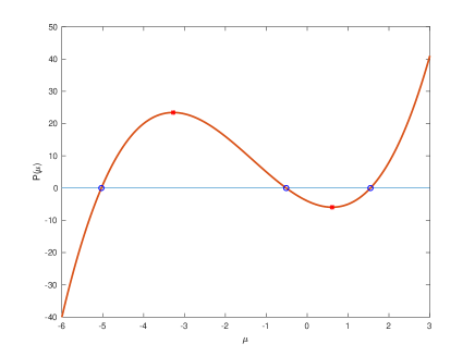
  Figure 1: Typical graph for $\mu\mapsto P(\mu)$, with its roots $\mu_{1}<\mu_{2}<\mu_{3}$ and local extrema $\mu_{\mathrm{max}}$, $\mu_{\mathrm{min}}$

  Coming back to the issue of counting the negative eigenvalues of $\mathscr{L}$, we are thus wondering whether or not $\lambda_{j}=\mu_{j}+m^{2}/2$ is negative. We already know that $\mu_{3}>\mu_{\mathrm{min}}>0$, hence $\mu_{3}>-m^{2}/2$ and we have at most 2 negative eigenvalues for each Fourier mode $m\neq 0$ such that $\sigma_{1,m}\neq 0$. To decide how many negative eigenvalues should be counted, we look at the sign of $P(-m^{2}/2)$ (see Fig. 1):

  • if $P(-m^{2}/2)>0$ then $\mu_{1}<-m^{2}/2<\mu_{2}$,

  • if $P(-m^{2}/2)=0$ then either $-m^{2}/2<\mu_{\mathrm{max}}$, in which case $\mu_{1}=-m^{2}/2<\mu_{2}$, or $-m^{2}/2>\mu_{\mathrm{max}}$, in which case $\mu_{2}=-m^{2}/2>\mu_{1}$,

  • if $P(-m^{2}/2)<0$ then either $-m^{2}/2<\mu_{\mathrm{max}}$, in which case $-m^{2}/2<\mu_{1}<\mu_{2}$, or $-m^{2}/2>\mu_{\mathrm{max}}$, in which case $\mu_{1}<\mu_{2}<-m^{2}/2$.

  However, we remark that

  $$\begin{array}[]{lll}P(-m^{2}/2)&=&-\displaystyle\frac{m^{6}}{8}+\displaystyle\frac{m^{4}(m^{2}-1)}{8}+\displaystyle\frac{m^{2}}{2}((k\cdot m)^{2}+\gammaup\sigma_{1,m}^{2})-\displaystyle\frac{m^{2}-1}{2}(k\cdot m)^{2}\\[8.5359pt] &=&-\displaystyle\frac{m^{4}}{8}\Big{(}1-4\displaystyle\frac{\gammaup\sigma_{1,m}^{2}}{m^{2}}\Big{)}+\displaystyle\frac{(k\cdot m)^{2}}{2}=-\displaystyle\frac{1}{8}(m^{4}-4(k\cdot m)^{2}-4m^{2}\gammaup\sigma^{2}_{1,m}),\end{array}$$ (56)

  where, by virtue of 9, $m\neq 0$ and $\sigma_{1_{m}}\neq 0$, $1>4\frac{\gammaup\sigma_{1,m}^{2}}{m^{2}}>0$.

  This can be combined together with

  $$P^{\prime}(-m^{2}/2)= 3\displaystyle\frac{m^{4}}{4}-\displaystyle\frac{m^{2}(m^{2}-1)}{2}-(k\cdot m)^{2}-\gammaup\sigma_{1,m}^{2}=\displaystyle\frac{m^{4}}{4}+\displaystyle\frac{m^{2}}{2}-(k\cdot m)^{2}-\gammaup\sigma_{1,m}^{2}$$

  $$= \frac{1}{4}\left(m^{4}-4(k\cdot m)^{2}-4m^{2}\gammaup\sigma_{1,m}^{2}\right)+m^{2}\gammaup\sigma_{1,m}^{2}+\frac{m^{2}}{2}-\gammaup\sigma_{1,m}^{2}$$

  $$= -2P(-m^{2}/2)+\frac{m^{2}}{2}+(m^{2}-1)\gammaup\sigma_{1,m}^{2}>-2P(-m^{2}/2).$$

  Finally,

  $$P^{\prime\prime}(-m^{2}/2)=-2m^{2}-1<0.$$

  As a consequence, $P(-m^{2}/2)<0$ implies $P^{\prime}(-m^{2}/2)>0$, while $P^{\prime\prime}(-m^{2}/2)<0$. This shows that $-m^{2}/2<\mu_{1}$. Therefore, in case iii), the only remaining possibility is the situation where $P(-m^{2}/2)<0$ with $-m^{2}/2<\mu_{1}<\mu_{2}$. As a conclusion, if $P(-m^{2}/2)<0$, all eigenvalues $\lambda_{j}$ are positive.

  Next, we claim that case ii) cannot occur. Indeed, $P(-m^{2}/2)=0$ if and only if

  $$(m^{2}-2k\cdot m)(m^{2}+2k\cdot m)=4m^{2}\gammaup\sigma^{2}_{1,m}.$$

  In particular, the term on the left hand side of this equality has to be positive. This is possible if and only if both factors, which belong to $\mathbb{Z}$, are positive. In this case, according to the sign of $k\cdot m$, one of them is $\geq m^{2}$ so that

  $$m^{2}\leq 4m^{2}\gammaup\sigma^{2}_{1,m}.$$

  This contradicts the smallness condition 9. Note that $P(-m^{2}/2)\neq 0$ implies $\lambda_{j}\neq 0$, i.e. $m$-modes with $m\neq 0$ and $\sigma_{1,m}\neq 0$ cannot generate elements of $\mathrm{Ker}(\mathscr{L})$.

  As a conclusion, negative eigenvalues only come from case i) and for each $m$-mode such that $P(-m^{2}/2)>0$ we have exactly one negative eigenvalue. Going back to 56, in this case, we have

  $$(m^{4}-4(k\cdot m)^{2})=(m^{2}-2k\cdot m)(m^{2}+2k\cdot m)<m^{2}4\gammaup\sigma_{1,m}^{2}<m^{2}$$

  owing to 9. This excludes the possibility that $m^{4}-4(k\cdot m)^{2}>0$, since we noticed above that whenever this term is positive, it is $\geq m^{2}$. Hence, case i) holds if and only if $m^{4}-4(k\cdot m)^{2}\leq 0$.

This ends the counting of the negative eigenvalues of $\mathscr{L}$ in Proposition 5.3. Note that the associated eigenspaces are spanned by

$$\Big{(}e^{im\cdot x},-\frac{ik\cdot m}{\lambda-m^{2}/2}e^{im\cdot x},e^{im\cdot x}\frac{\sigma_{1,m}\gamma(2\uppi)^{d}(-\Delta_{z})^{-1/2}\sigma_{2}}{\lambda-1/2},0\Big{)}.$$

The discussion has permitted us to find the elements of $\mathrm{Ker}(\mathscr{L})$. To be specific, the equation $\mathscr{L}X=0$ yields $\pi=0$ and the following relations for the Fourier coefficients

$$\begin{array}[]{l}\displaystyle\frac{m^{2}}{2}p_{m}-ik\cdot mq_{m}=0,\\[8.5359pt] \displaystyle\frac{\phi_{m}}{2}+(2\uppi)^{d}\gamma(-\Delta)^{-1/2}\sigma_{2}\sigma_{1,m}q_{m}=0,\\[8.5359pt] \displaystyle\frac{m^{2}}{2}q_{m}+ik\cdot mp_{m}+(2\uppi)^{d}\gamma\sigma_{1,m}\displaystyle\int(-\Delta)^{-1/2}\sigma_{2}\phi_{m}\,{\mathrm{d}}z=0.\end{array}$$

We have seen that the mode $m=0$ gives rise the eigenspace spanned by $(0,\mathbf{1},0,0)$. For $m\neq 0$, elements of $\mathrm{Ker}(\mathscr{L})$ can be obtained only in the case $\sigma_{1,m}=0$. Moreover, the condition $m^{2}=\pm 2k\cdot m$ has to be fulfilled. In such a case, $(e^{im\cdot x},\mp ie^{im\cdot x},0,0)\in\mathrm{Ker}(\mathscr{L})$.

Finally, it remains to prove that $\sigma_{\mathrm{ess}}(\mathscr{L})=\left\{\frac{1}{2}\right\}$. We have already noticed that $\frac{1}{2}$ lies in $\sigma_{\mathrm{ess}}(\mathscr{L})$. Suppose, by contradiction, that there exists $\lambda\in\sigma_{\mathrm{ess}}(\mathscr{L})$ with $\lambda\neq\frac{1}{2}$. Hence, by Weyl’s criterion [46, Theorem B.14], there exists a sequence $(X_{\nu})_{\nu\in\mathbb{N}}$ with $X_{\nu}=(q_{\nu},p_{\nu},\phi_{\nu},\pi_{\nu})\in D(\mathscr{L})$ such that, as $\nu$ goes to $\infty$,

$$\|(\mathscr{L}-\lambda I)X_{\nu}\|\to 0,\quad\|X_{\nu}\|=1\text{ and }X_{\nu}\rightharpoonup 0\textrm{ weakly in $\mathscr{V}$}.$$ (57)

Since $\lambda\neq\tfrac{1}{2}$ and $\lambda\neq 2c^{2}$, from 53 and 57 we have

$$\|\pi_{\nu}\|_{L^{2}(\mathbb{T}^{d};L^{2}(\mathbb{R}^{n}))}\to 0\text{ and }\phi_{\nu}=-\left(\frac{1}{2}-\lambda\right)^{-1}\gamma(-\Delta)^{-1/2}\sigma_{2}\sigma_{1}\star q_{\nu}+\varepsilon_{\nu}$$

with $\varepsilon_{\nu}\in L^{2}(\mathbb{T}^{d};L^{2}(\mathbb{R}^{n}))$ such that $\lim_{\nu\to\infty}\|\varepsilon_{\nu}\|_{L^{2}(\mathbb{T}^{d};L^{2}(\mathbb{R}^{n}))}=0$. This leads to

$$\left\|-\frac{1}{2}\Delta_{x}q_{\nu}-\lambda q_{\nu}+k\cdot\nabla_{x}p_{\nu}-\frac{\gamma^{2}\kappa}{1/2-\lambda}\Sigma\star q_{\nu}+\gamma\sigma_{1}\star\left(\displaystyle\int_{\mathbb{R}^{n}}(-\Delta)^{-1/2}\sigma_{2}\varepsilon_{\nu}\,{\mathrm{d}}z\right)\right\|_{L^{2}(\mathbb{T}^{d})}\xrightarrow[\nu\to\infty]{}0,$$

$$\left\|-\dfrac{1}{2}\Delta_{x}p_{\nu}-\lambda p_{\nu}-k\cdot\nabla_{x}q_{\nu}\right\|_{L^{2}(\mathbb{T}^{d})}\xrightarrow[\nu\to\infty]{}0.$$

Using the fact that the sequence $((q_{\nu},p_{\nu},\varepsilon_{\nu}))_{\nu\in\mathbb{N}}$ is bounded in $L^{2}(\mathbb{T}^{d})\times L^{2}(\mathbb{T}^{d})\times L^{2}(\mathbb{T}^{d};L^{2}(\mathbb{R}^{n}))$, we deduce that $(q_{\nu},p_{\nu})_{\nu\in\mathbb{N}}$ is bounded in $H^{2}(\mathbb{T}^{d})\times H^{2}(\mathbb{T}^{d})$. Indeed, reasoning on Fourier series, this amounts to estimate

$$\begin{array}[]{l}\displaystyle\sum_{m\in\mathbb{Z}^{d}}|m|^{4}(|q_{\nu,m}|^{2}+|p_{\nu,m}|^{2})\\ \qquad\leq 2\displaystyle\sum_{m\in\mathbb{Z}^{d}}\big{(}|m^{2}q_{\nu,m}+2ik\cdot mp_{\nu,m}|^{2}+|m^{2}p_{\nu,m}-2ik\cdot mq_{\nu,m}|^{2})\\ \qquad\qquad\qquad+8\displaystyle\sum_{m\in\mathbb{Z}^{d}}(|k\cdot mp_{\nu,m}|^{2}+|k\cdot mq_{\nu,m}|^{2})\\ \qquad\leq 2\big{\|}-\Delta_{x}q_{\nu}+2k\cdot\nabla_{x}p_{\nu}\big{\|}_{L^{2}(\mathbb{T}^{d})}+2\big{\|}-\Delta_{x}p_{\nu}-2k\cdot\nabla_{x}q_{\nu}\big{\|}_{L^{2}(\mathbb{T}^{d})}\\ \qquad\qquad\qquad+\displaystyle\frac{4}{\delta}|k|^{4}\displaystyle\sum_{m\in\mathbb{Z}^{d}}\big{(}|q_{\nu,m}|^{2}+|p_{\nu,m}|^{2}\big{)}+4\delta\displaystyle\sum_{m\in\mathbb{Z}^{d}}|m|^{4}(|q_{\nu,m}|^{2}+|p_{\nu,m}|^{2}).\end{array}.$$

Choosing $0<\delta<1/4$ and using the already known estimates, we conclude that $\|\Delta_{x}q_{\nu}\|^{2}_{L^{2}}+\|\Delta_{x}p_{\nu}\|^{2}_{L^{2}}=\sum_{m\in\mathbb{Z}^{d}}|m|^{4}\big{(}|q_{\nu,m}|^{2}+|p_{\nu,m}|^{2}\big{)}$ is bounded, uniformly with respect to $\nu$. Hence, because of the compact Sobolev embedding of $H^{2}(\mathbb{T}^{d})$ into $L^{2}(\mathbb{T}^{d})$, we have that $(q_{\nu},p_{\nu})_{\nu\in\mathbb{N}}$ has a (strongly) convergent subsequence in $L^{2}(\mathbb{T}^{d})\times L^{2}(\mathbb{T}^{d})$. As a consequence, the sequence $(X_{\nu})_{\nu\in\mathbb{N}}$ has a convergent subsequence in $\mathscr{V}$, which contradicts 57.  

A consequence of Proposition 5.3 is that $0$ is an isolated eigenvalue of $\mathscr{L}$. Since the restriction of $\mathscr{L}$ to the subspace $(\mathrm{Ker}(\mathscr{L}))^{\perp}$ is, by definition, injective, it makes sense to define on it its inverse $\mathscr{L}^{-1}$, with domain $\mathrm{Ran}(\mathscr{L})\subset(\mathrm{Ker}(\mathscr{L}))^{\perp}\subset\mathscr{V}$. In fact, 0 being an isolated eigenvalue, $\mathrm{Ran}(\mathscr{L})$ is closed and coincides with $(\mathrm{Ker}(\mathscr{L}))^{\perp}$, [46, Section B.4]. This can be shown by means of spectral measures. Given $X\in(\mathrm{Ker}(\mathscr{L}))^{\perp}$, the support of the associated spectral measure $\,{\mathrm{d}}\mu_{X}$ does not meet the interval $(-\epsilon,+\epsilon)$ for $\epsilon>0$ small enough, independent of $X$. Accordingly, we get

$$\|\mathscr{L}X\|^{2}=\displaystyle\int_{-\infty}^{+\infty}\lambda^{2}\,{\mathrm{d}}\mu_{X}(\lambda)=\displaystyle\int_{|\lambda|\geq\epsilon}\lambda^{2}\,{\mathrm{d}}\mu_{X}(\lambda)\geq\epsilon^{2}\|X\|^{2}.$$

In particular, the Fredholm alternative applies: for any $Y\in(\mathrm{Ker}(\mathscr{L}))^{\perp}$, there exists a unique $X\in(\mathrm{Ker}(\mathscr{L}))^{\perp}$ such that $\mathscr{L}X=Y$. We will denote $X=\mathscr{L}^{-1}Y$.

For further purposes, let us set

$$X_{0}=(0,\mathbf{1},0,0)\in\mathrm{Ker}(\mathscr{L})\textrm{ and }Y_{0}={\color[rgb]{0,0,0}\mathscr{J}X_{0}}=(\mathbf{1},0,0,0).$$

Note that $Y_{0}\in(\mathrm{Ker}(\mathscr{L}))^{\perp}$, so that it makes sense to consider the equation

$$\mathscr{L}U_{0}=Y_{0}.$$

We find

$$\pi_{m}=0,\quad\phi_{m}=-2\gamma(2\uppi)^{d}(-\Delta)^{-1/2}\sigma_{2}\sigma_{1,m}q_{m},\quad m^{2}p_{m}=2ik\cdot mq_{m},$$

and

$$m^{2}q_{m}+2ik\cdot mp_{m}+2\gamma(2\uppi)^{d}\sigma_{1,m}\displaystyle\int(-\Delta)^{-1/2}\sigma_{2}\phi_{m}\,{\mathrm{d}}z=\delta_{0,m}.$$

It yields, for $m\neq 0$, $(\frac{m^{4}}{4}-(k\cdot m)^{2}-\gammaup|\sigma_{1,m}|^{2}m^{2}\Big{)}q_{m}=0$ and $q_{0}=-\frac{1}{2\gamma^{2}(2\uppi)^{2d}|\sigma_{1,0}|^{2}\kappa}$. Therefore, we can set

$$U_{0}=\mathscr{L}^{-1}Y_{0}=-\displaystyle\frac{1}{2\gamma^{2}(2\uppi)^{2d}|\sigma_{1,0}|^{2}\kappa}\big{(}\mathbf{1},0,-2\gamma(2\uppi)^{d}(-\Delta)^{-1/2}\sigma_{2}\sigma_{1,0},0\big{)},$$

solution of $\mathscr{L}U_{0}=Y_{0}$ such that $U_{0}\in(\mathrm{Ker}(\mathscr{L}))^{\perp}$. We note that

$$(U_{0},Y_{0})=-\displaystyle\frac{1}{2\gamma^{2}(2\uppi)^{d}|\sigma_{1,0}|^{2}\kappa}<0.$$ (58)

5.3 Reformulation of the eigenvalue problem, and counting theorem

The aim of the section is to introduce several reformulations of the eigenvalue problem. This will allow us to make use of general counting arguments, set up by [9, 46, 47].

Proposition 5.4

Let us set $\mathscr{M}=-\mathscr{J}\mathscr{L}\mathscr{J}$. The coupled system

$$\mathscr{M}Y=-\lambda X,\qquad\mathscr{L}X=\lambda Y,$$ (59)

admits a solution with $\lambda\neq 0$, $X\in D(\mathscr{L})\smallsetminus\{0\}$, $Y\in D(\mathscr{J}\mathscr{L}\mathscr{J})\smallsetminus\{0\}$ iff there exists two vectors $X_{\pm}\in D(\mathbb{L})\smallsetminus\{0\}$ that satisfy $\mathbb{L}X_{\pm}=\pm\lambda X_{\pm}$.

Let $\mathscr{P}$ stand for the orthogonal projection from $\mathscr{V}$ to $(\mathrm{Ker}(\mathscr{L}))^{\perp}\subset\mathscr{V}$.

Proposition 5.5

Let us set $\mathbb{A}=\mathscr{P}\mathscr{M}\mathscr{P}$ and $\mathbb{K}=\mathscr{P}\mathscr{L}^{-1}\mathscr{P}$. Let us define the following Hilbert space

$$\mathscr{H}=D(\mathscr{M})\cap(\mathrm{Ker}(\mathscr{L}))^{\perp}\subset\mathscr{V}.$$

The coupled system 59 has a pair of non trivial solutions $(\pm\lambda,X,\pm Y)$, with $\lambda\neq 0$ iff the generalized eigenproblem

$$\mathbb{A}W=\alpha\mathbb{K}W,\qquad W\in\mathscr{H},$$ (60)

admits the eigenvalue $\alpha=-\lambda^{2}\neq 0$, with at least two linearly independent eigenfunctions.

Recall that the plane wave solution obtained Section 2.1 is spectrally stable, if the spectrum of $\mathbb{L}$ is contained in $i\mathbb{R}$. In view of Propositions 5.4 and 5.5, this happens if and only if all the eigenvalues of the generalized eigenproblem 60 are real and positive. In other words, the presence of spectrally unstable directions corresponds to the existence of negative eigenvalues or complex but non real eigenvalues of the generalized eigenproblem 60.

Our goal is then to count the eigenvalues $\alpha$ of the generalized eigenvalue problem 60. In particular we define the following quantities:

• $N^{-}_{n}$, the number of negative eigenvalues

• $N^{0}_{n}$, the number of eigenvalues zero

• $N^{+}_{n}$, the number of positive eigenvalues

of 60, counted with their algebraic multiplicity, the eigenvectors of which are associated to non-positive values of the the quadratic form $W\mapsto(\mathbb{K}W|W)=(\mathscr{L}^{-1}\mathscr{P}W|\mathscr{P}W)$. Moreover, let $N_{C^{+}}$ be the number of eigenvalues $\alpha\in\mathbb{C}$ with $\mathrm{Im}(\alpha)>0$.

As pointed out above, the eigenvalues counted by $N^{-}_{n}$ and $N_{C^{+}}$ correspond to cases of instabilities for the linearized problem 38. Note that to prove the spectral stability, it is enough to show that the generalized eigenproblem 60 does not have negative eigenvalues and $N_{C^{+}}=0$. Indeed, as a consequence of Propositions 5.4 and 5.5 and Lemma 5.1, if $\alpha\in\mathbb{C}\smallsetminus\mathbb{R}$ is an eigenvalue of 60, then $\bar{\alpha}$ is an eigenvalue too. Hence, if $N_{C^{+}}=0$, then the generalized eigenproblem 60 does not have solutions in $\mathbb{C}\smallsetminus\mathbb{R}$.

Finally, for using the counting argument introduce by Chugunova and Pelinovsky in [9], we need the following information on the essential spectrum of $\mathbb{A}$, see [47, Lemma 2-(H1’) and Lemma 4].

Lemma 5.6

Let $\mathscr{M}=-\mathscr{J}\mathscr{L}\mathscr{J}$ be defined on $\mathscr{V}$. Then $\sigma_{\mathrm{ess}}(\mathscr{M})=[0,+\infty)$. Let $\mathbb{A}=\mathscr{P}\mathscr{M}\mathscr{P}$ and $\mathbb{K}=\mathscr{P}\mathscr{L}^{-1}\mathscr{P}$ be defined on $\mathscr{H}$. Then $\sigma_{\mathrm{ess}}(\mathbb{A})=[0,+\infty)$ and we can find $\delta_{*},d_{*}>0$ such that for any real number $0<\delta<\delta_{*}$, $\mathbb{A}+\delta\mathbb{K}$ admits a bounded inverse and we have $\sigma_{\mathrm{ess}}(\mathbb{A}+\delta\mathbb{K})\subset[d_{*}\delta,+\infty)$.

Proof. We check that

$$\mathscr{J}\mathscr{L}\mathscr{J}X=\begin{pmatrix}\displaystyle\frac{\Delta_{x}q}{2}-k\cdot\nabla_{x}p\\ \displaystyle\frac{\Delta_{x}p}{2}+k\cdot\nabla_{x}q+2c\gamma\sigma_{1}\star\displaystyle\int(-\Delta_{z})^{-1/2}\sigma_{2}(-\Delta_{z})^{1/2}\pi\,{\mathrm{d}}z\\ 2c^{2}\Delta_{z}\phi\\ 2c^{2}\displaystyle\frac{\Delta_{z}\pi}{2}+2c\gamma\sigma_{2}\sigma_{1}\star p\end{pmatrix}.$$

As a matter of fact, for any $\phi\in H^{2}(\mathbb{R}^{n})$, the vector $X_{e}=(0,0,\phi,0)$ lies in $(\mathrm{Ker}(\mathscr{L}))^{\perp}$ and satisfies

$$\mathscr{J}\mathscr{L}\mathscr{J}X_{e}=\begin{pmatrix}0\\ 0\\ 2c^{2}\Delta_{z}\phi\\ 0\end{pmatrix}\in(\mathrm{Ker}(\mathscr{L}))^{\perp}.$$

Consequently $\mathscr{M}X_{e}=\mathbb{A}X_{e}=-\mathscr{J}\mathscr{L}\mathscr{J}X_{e}=(0,0,-2c^{2}\Delta_{z}\phi,0)$. It indicates that a Weyl sequence for $\mathbb{A}-\lambda\mathbb{I}$, $\lambda>0$, can be obtained by adapting a Weyl sequence for $(-\Delta_{z}-\mu\mathbb{I})$, $\mu>0$. Let us consider a sequence of smooth functions $\zeta_{\nu}\in C^{\infty}_{c}(\mathbb{R}^{n})$ such that $\mathrm{supp}(\zeta_{\nu})\subset B(0,\nu+1)$, $\zeta_{\nu}(z)=1$ for $x\in B(0,\nu)$ and $\|\nabla_{z}\zeta_{\nu}\|_{L^{\infty}(\mathbb{R}^{n})}\leq C_{0}<\infty$, $\|D_{z}^{2}\zeta_{\nu}\|_{L^{\infty}(\mathbb{R}^{n})}\leq C_{0}<\infty$, uniformly with respect to $\nu\in\mathbb{N}$. We set $\phi_{\nu}(z)=\zeta_{\nu}(z)e^{i\xi\cdot z/(\sqrt{2}c)}$ for some $\xi\in\mathbb{R}^{n}$. We get

$$(-|\xi|^{2}-2c^{2}\Delta_{z})\phi_{\nu}(z)={\color[rgb]{0,0,0}-}e^{i\xi\cdot z/(\sqrt{2}c)}\Big{(}\displaystyle\frac{2i}{\sqrt{2}c}\xi\cdot\nabla_{z}\zeta_{\nu}+2c^{2}\Delta_{z}\zeta_{\nu}\Big{)}(z),$$

which is thus bounded in $L^{\infty}(\mathbb{R}^{n})$ and supported in $B(0,\nu+1)\smallsetminus B(0,\nu)$. It follows that $\|(-|\xi|^{2}-2c^{2}\Delta_{z})\phi_{\nu}\|^{2}_{L^{2}(\mathbb{R}^{n})}\lesssim\nu^{n-1}$, while $\|\phi_{\nu}\|^{2}_{L^{2}(\mathbb{R}^{n})}\gtrsim\nu^{n}$. Accordingly, we obtain $\frac{\|\phi_{\nu}\|^{2}_{L^{2}(\mathbb{R}^{n})}}{\|(-|\xi|^{2}-2c^{2}\Delta_{z})\phi_{\nu}\|^{2}_{L^{2}(\mathbb{R}^{n})}}\gtrsim\nu\to\infty$ as $\nu\to\infty$. Therefore, $\phi_{\nu}$ equally provides a Weyl sequence for $\mathscr{M}-|\xi|^{2}\mathbb{I}$ and $\mathbb{A}-|\xi|^{2}\mathbb{I}$, showing the inclusions $[0,\infty)\subset\sigma_{\mathrm{ess}}(\mathscr{M})$ and $[0,\infty)\subset\sigma_{\mathrm{ess}}(\mathbb{A})$.

Next, let $\lambda\notin[0,\infty)$. We suppose that we can find a Weyl sequence $(X_{\nu})_{\nu\in\mathbb{N}}$ for $\mathscr{M}$, such that

$$\begin{array}[]{lll}\mathscr{M}X_{\nu}-\lambda X_{\nu}&=&\begin{pmatrix}-\lambda q_{\nu}-\displaystyle\frac{\Delta_{x}q_{\nu}}{2}+k\cdot\nabla_{x}p_{\nu}\\ -\lambda p_{\nu}-\displaystyle\frac{\Delta_{x}p_{\nu}}{2}-k\cdot\nabla_{x}q_{\nu}-2c\gamma\sigma_{1}\star\displaystyle\int(-\Delta_{z})^{-1/2}\sigma_{2}(-\Delta_{z})^{1/2}\pi_{\nu}\,{\mathrm{d}}z\\ -\lambda\phi_{\nu}-2c^{2}\Delta_{z}\phi_{\nu}\\ -\lambda\pi_{\nu}-2c^{2}\Delta_{z}\pi_{\nu}-2c\gamma\sigma_{2}\sigma_{1}\star p_{\nu}\end{pmatrix}\\ &=&\begin{pmatrix}q^{\prime}_{\nu}\\ p^{\prime}_{\nu}\\ \phi^{\prime}_{\nu}\\ \pi^{\prime}_{\nu}\end{pmatrix}\xrightarrow[\nu\to\infty]{}0,\end{array}$$

with, moreover, $\|X_{\nu}\|=1$ and $X_{\nu}\rightharpoonup 0$ weakly in $\mathscr{V}$. In particular, we can set

$$\widehat{\phi_{\nu}}(x,\xi)=\frac{\widehat{\phi^{\prime}_{\nu}}(x,\xi)}{2c^{2}|\xi|^{2}-\lambda}.$$ (61)

It defines a sequence which tends to 0 strongly $L^{2}(\mathbb{T}^{d}\times\mathbb{R}^{n})$ since, writing $\lambda=a+ib\in\mathbb{C}\smallsetminus[0,\infty)$, we get $|2c^{2}|\xi|^{2}-\lambda|^{2}=|2c^{2}|\xi|^{2}-a|^{2}+b^{2}$ which is $\geq b^{2}>0$ when $\lambda\notin\mathbb{R}$, and, in case $b=0$, $\geq a^{2}>0$. Similarly, we can write

$$\widehat{\pi_{\nu}}(x,\xi)=\underbrace{\displaystyle\frac{\widehat{\pi^{\prime}_{\nu}}(x,\xi)}{2c^{2}|\xi|^{2}-\lambda}}_{=h_{\nu}(x,\xi)\in L^{2}(\mathbb{T}^{d}\times\mathbb{R}^{n})}+\underbrace{\displaystyle\frac{2c\gamma\widehat{\sigma_{2}}(\xi)}{2c^{2}|\xi|^{2}-\lambda}}_{\in L^{2}(\mathbb{R}^{n})}\sigma_{1}\star p_{\nu},$$ (62)

where $h_{\nu}$ tends to 0 strongly $L^{2}(\mathbb{T}^{d}\times\mathbb{R}^{n})$. We are led to the system

$$\begin{array}[]{l}\begin{pmatrix}-\Big{(}\lambda+\displaystyle\frac{\Delta_{x}}{2}\Big{)}q_{\nu}+k\cdot\nabla_{x}p_{\nu}\\ -k\cdot\nabla_{x}q_{\nu}-\Big{(}\lambda+\displaystyle\frac{\Delta_{x}}{2}\Big{)}p_{\nu}-4c^{2}\gamma^{2}\displaystyle\int\displaystyle\frac{|\widehat{\sigma_{2}}|^{2}}{(2\uppi)^{n}(2c^{2}|\xi|^{2}-\lambda)}\,{\mathrm{d}}\xi\times\Sigma\star p_{\nu}\end{pmatrix}\\[11.38092pt] \hskip 85.35826pt=\begin{pmatrix}q^{\prime}_{\nu}\\ p^{\prime}_{\nu}-2c\gamma\sigma_{1}\star\displaystyle\int\displaystyle\frac{\widehat{\sigma_{2}}(\xi)}{|\xi|}h_{\nu}(x,\xi)\frac{\,{\mathrm{d}}\xi}{(2\uppi)^{n}}\end{pmatrix}\xrightarrow[\nu\to\infty]{}0.\end{array}$$ (63)

Reasoning as in the proof of Proposition 5.3-1), we conclude that $X_{\nu}$ converges strongly to 0 in $\mathscr{V}$, a contradiction. Hence, $\lambda\in\mathbb{C}\smallsetminus[0,\infty)$ cannot belong to $\sigma_{\mathrm{ess}}(\mathscr{M})$ and the identification $\sigma_{\mathrm{ess}}(\mathscr{M})=[0,\infty)$ holds.

Proposition 5.3-3) identifies $\mathrm{Ker}(\mathscr{L})$. Let us introduce the mapping

$$\widetilde{\mathscr{P}}:\begin{pmatrix}q\\ p\end{pmatrix}\in L^{2}(\mathbb{T}^{d})\times L^{2}(\mathbb{T}^{d})\longmapsto\begin{pmatrix}\displaystyle\sum_{m\in\mathscr{K}_{*},\ k\cdot m>0}(q_{m}-ip_{m})e^{im\cdot x}+\displaystyle\sum_{m\in\mathscr{K}_{*},\ k\cdot m<0}(q_{m}+ip_{m})e^{im\cdot x}\\ p_{0}+i\displaystyle\sum_{m\in\mathscr{K}_{*},\ k\cdot m>0}(q_{m}-ip_{m})e^{im\cdot x}-i\displaystyle\sum_{m\in\mathscr{K}_{*},\ k\cdot m<0}(q_{m}+ip_{m})e^{im\cdot x}\end{pmatrix}.$$

Then,

$$X=\begin{pmatrix}q\\ p\\ \phi\\ \pi\end{pmatrix}\longmapsto\begin{pmatrix}\widetilde{\mathscr{P}}\begin{pmatrix}q\\ p\end{pmatrix}\\ 0\\ 0\end{pmatrix}$$

is the projection of $\mathscr{V}$ on $\mathrm{Ker}(\mathscr{L})$. Accordingly, we realize that $\mathscr{P}$ does not modify the last two components of a vector $X=(q,p,\phi,\pi)\in\mathscr{V}$, and for $X\in(\mathrm{Ker}(\mathscr{L}))^{\perp}$, we have $p_{0}=0$, and $q_{m}=\pm ip_{m}$ for any $m\in\mathscr{K}_{*}$, depending on the sign of $k\cdot m$.

Now, let $\lambda\in\mathbb{C}\smallsetminus[0,\infty)$ and suppose that we can exhibit a Weyl sequence $(X_{\nu})_{\nu\in\mathbb{N}}$ for $\mathbb{A}-\lambda\mathbb{I}$: $X_{\nu}\in\mathscr{H}\subset(\mathrm{Ker}(\mathscr{L}))^{\perp}$, $\mathscr{P}X_{\nu}=X_{\nu}$, $\|X_{\nu}\|=1$, $X_{\nu}\rightharpoonup 0$ in $\mathscr{V}$ and $\lim_{\nu\to\infty}\|(\mathbb{A}-\lambda\mathbb{I})X_{\nu}\|=0$. We can apply the same reasoning as before for the last two components of $(\mathbb{A}-\lambda\mathbb{I})X_{\nu}$; it leads to 61 and 62, where, using $\lambda\notin[0,\infty)$, $\phi_{\nu}$ and $h_{\nu}$ converge strongly to 0 in $L^{2}(\mathbb{T}^{d}\times\mathbb{R}^{n})$. We arrive at the following analog to 63

$$\begin{array}[]{l}(\mathbb{I}-\widetilde{\mathscr{P}})\begin{pmatrix}-\Big{(}\lambda+\displaystyle\frac{\Delta_{x}}{2}\Big{)}q_{\nu}+k\cdot\nabla_{x}p_{\nu}\\ -k\cdot\nabla_{x}q_{\nu}-\Big{(}\lambda+\displaystyle\frac{\Delta_{x}}{2}\Big{)}p_{\nu}-4c^{2}\gamma^{2}\displaystyle\int\displaystyle\frac{|\widehat{\sigma_{2}}|^{2}}{(2\uppi)^{n}(2c^{2}|\xi|^{2}-\lambda)}\,{\mathrm{d}}\xi\times\Sigma\star p_{\nu}\end{pmatrix}\\[11.38092pt] \hskip 85.35826pt=\begin{pmatrix}q^{\prime}_{\nu}\\ p^{\prime}_{\nu}\end{pmatrix}-(\mathbb{I}-\widetilde{\mathscr{P}})\begin{pmatrix}0\\ 2c\gamma\sigma_{1}\star\displaystyle\int\displaystyle\frac{\widehat{\sigma_{2}}(\xi)}{|\xi|}h_{\nu}(x,\xi)\frac{\,{\mathrm{d}}\xi}{(2\uppi)^{n}}\end{pmatrix}\xrightarrow[\nu\to\infty]{}0.\end{array}$$ (64)

In order to derive from 64 an estimate in a positive Sobolev space as we did in the proof of Proposition 5.3-1), we should consider the Fourier coefficients arising from $-\frac{1}{2}\Delta_{x}q_{\nu}+k\cdot\nabla_{x}p_{\nu}$ and $-\frac{1}{2}\Delta_{x}p_{\nu}-k\cdot\nabla_{x}q_{\nu}$, namely $Q_{m}=\frac{m^{2}}{2}q_{\nu,m}+ik\cdot mp_{\nu,m}$ and $P_{m}=\frac{m^{2}}{2}p_{\nu,m}-ik\cdot mq_{\nu,m}$. Only the coefficients belonging to $\mathscr{K}_{*}$ are affected by the action of $\widetilde{\mathscr{P}}$, which leads to $Q_{m}-(Q_{m}\mp iP_{m})=\pm iP_{m}$ and $P_{m}\mp i(Q_{m}\mp iP_{m})=\mp iQ_{m}$, according to the sign of $k\cdot m$. However, we bear in mind that $q_{m}=\pm ip_{m}$ when $m\in\mathscr{K}_{*}$ with $\pm k\cdot m>0$. Hence, for coefficients in $\mathscr{K}_{*}$, the contributions of the differential operators reduces to $\pm im^{2}p_{m}=\pm m^{2}q_{m}$ and $\mp im^{2}q_{m}=\pm m^{2}p_{m}$, respectively. Note also that for these coefficients there is no contributions coming from the convolution with $\sigma_{1}$ in 64 since $\sigma_{1,m}=0$ for $m\in\mathscr{K}_{*}$. Therefore, reasoning as in the proof of Proposition 5.3-1) for coefficients $m\in\mathbb{Z}^{d}\smallsetminus\mathscr{K}_{*}$, we can obtain a uniform bound on $\sum_{m\in\mathbb{Z}^{d}}|m|^{4}(|q_{\nu,m}|^{2}+|p_{\nu,m}|^{2})$, which provides a uniform $H^{2}$ bound on $q_{\nu}$ and $p_{\nu}$, leading eventually to a contradiction. We conclude that $\sigma_{\mathrm{ess}}(\mathbb{A})=[0,\infty)$.

Let $\delta>0$ and consider the shifted operator $\mathbb{A}+\delta\mathbb{K}$. As a consequence of Lemma 5.10, we will see that $\mathrm{Ker}(\mathbb{A}+\delta\mathbb{K})=\{0\}$ for any $\delta>0$: 0 is not an eigenvalue for $\mathbb{A}+\delta\mathbb{K}$; let us justify it does not belong to the essential spectrum neither. To this end, we need to detail the expression of the operator $\mathbb{K}$. Given $X\in\mathscr{H}$, we wish to find $X^{\prime}\in\mathscr{H}$ satisfying

$$\mathscr{L}X^{\prime}=\begin{pmatrix}-\displaystyle\frac{1}{2}\Delta_{x}q^{\prime}+k\cdot\nabla_{x}p^{\prime}+\gamma\sigma_{1}\star\left(\displaystyle\int_{\mathbb{R}^{n}}(-\Delta)^{-1/2}\sigma_{2}\phi^{\prime}\,{\mathrm{d}}z\right)\\ -\displaystyle\dfrac{1}{2}\Delta_{x}p^{\prime}-k\cdot\nabla_{x}q^{\prime}\\ \displaystyle\frac{1}{2}\phi^{\prime}+\gamma(-\Delta)^{-1/2}\sigma_{2}\sigma_{1}\star q^{\prime}\\ \displaystyle\frac{\pi^{\prime}}{2}\end{pmatrix}=X.$$

We infer $\pi^{\prime}=2\pi$ and the relation $\phi^{\prime}=2\phi-2\gamma(-\Delta_{z})^{-1/2}\sigma_{2}\sigma_{1}\star q^{\prime}$. In turn, the Fourier coefficients of $q^{\prime},p^{\prime}$ are required to satisfy

$$\begin{pmatrix}m^{2}/2-2\gamma^{2}\kappa(2\uppi)^{2d}|\sigma_{1,m}|^{2}&ik\cdot m\\ -ik\cdot m&m^{2}/2\end{pmatrix}\begin{pmatrix}q^{\prime}_{m}\\ p^{\prime}_{m}\end{pmatrix}=\begin{pmatrix}q_{m}-2\gamma(2\uppi)^{d}\sigma_{1,m}\displaystyle\int(-\Delta)^{-1/2}\sigma_{2}\phi_{m}\,{\mathrm{d}}z\\ p_{m}\end{pmatrix}.$$

When $m\neq 0$, $m\notin\mathscr{K}_{*}$, the matrix of this system has its determinant equal to

$$\mathrm{det}=\frac{m^{4}}{4}\big{(}1-4\gamma^{2}\kappa(2\uppi)^{2d}\frac{|\sigma_{1,m}|^{2}}{m^{2}}\big{)}-(k\cdot m)^{2}.$$

Owing to 9, since $(k\cdot m)^{2}$ takes values in $\mathbb{N}$, it does not vanish and we obtain $q^{\prime}_{m},p^{\prime}_{m}$ by solving the system

$$\begin{array}[]{l}q^{\prime}_{m}=\displaystyle\frac{1}{\mathrm{det}}\left(\displaystyle\frac{m^{2}}{2}\Big{(}q_{m}-2\gamma(2\uppi)^{d}\sigma_{1,m}\displaystyle\int(-\Delta)^{-1/2}\sigma_{2}\phi_{m}\,{\mathrm{d}}z\Big{)}-ik\cdot mp_{m}\right),\\ p^{\prime}_{m}=\displaystyle\frac{1}{\mathrm{det}}\left(\displaystyle+ik\cdot m\Big{(}q_{m}-2\gamma(2\uppi)^{d}\sigma_{1,m}\displaystyle\int(-\Delta)^{-1/2}\sigma_{2}\phi_{m}\,{\mathrm{d}}z\Big{)}+\Big{(}\displaystyle\frac{m^{2}}{2}-2\gamma^{2}\kappa(2\uppi)^{2d}|\sigma_{1,m}|^{2}\Big{)}p_{m}\right).\end{array}$$

If $m\in\mathscr{K}_{*}$ we find a solution in $(\mathrm{Ker}(\mathscr{L}))^{\perp}$ by setting $p^{\prime}_{m}=\frac{p_{m}}{m^{2}}$, $q^{\prime}_{m}=\pm ip^{\prime}_{m}$, according to the sign of $k\cdot m$; if $m=0$, we set $p^{\prime}_{0}=0$ and $q_{0}^{\prime}=\frac{1}{2\gamma^{2}\kappa(2\uppi)^{2d}|\sigma_{1,0}|^{2}}\big{(}q_{0}-2\gamma(2\uppi)^{d}\sigma_{1,0}\int(-\Delta)^{-1/2}\sigma_{2}\phi_{0}\,{\mathrm{d}}z\big{)}$. This defines $X^{\prime}=\mathbb{K}X$.

Therefore, the last two components of $(\mathbb{A}+\delta\mathbb{K}-\lambda\mathbb{I})X$ read

$$\begin{array}[]{l}(2\delta-\lambda)\phi-2c^{2}\Delta_{z}\phi-2\delta\gamma(-\Delta)^{-1/2}\sigma_{2}\sigma_{1}\star q^{\prime},\\ (2\delta-\lambda)\pi-\displaystyle\frac{1}{2}\Delta_{z}\pi-\gamma\sigma_{2}\sigma_{1}\star p^{\prime}.\end{array}$$

Hence, when $\lambda$ does not belong to $[2\delta,\infty)$, we can repeat the analysis performed above to establish that $\lambda\notin\sigma_{\mathrm{ess}}(\mathbb{A}+\delta\mathbb{K})$. In particular the essential spectrum of $\mathbb{A}$ has been shifted away from 0.  

We are now able to apply the results of Chugunova and Pelinovsky [9] (see also [47]), to obtain the following.

Theorem 5.7

[9, Theorem 1] Let $\mathscr{L}$ be defined by 51. Suppose 9. With the operators $\mathscr{M},\mathbb{A},\mathbb{K}$ defined as in Propositions 5.4-5.5, the following identity holds

$$N^{-}_{n}+N^{0}_{n}+N^{+}_{n}+N_{C^{+}}=n(\mathscr{L}).$$

Let us now detail the proof of Proposition 5.4 and 5.5, adapted from [47, Prop. 1 & Prop. 3].

Proof of Propositions 5.4 and  5.5. The goal is to establish connections between the following three problems:

• the eigenvalue problem $\mathbb{L}X=\lambda X$, with $\mathbb{L}=\mathscr{J}\mathscr{L}$,

• the coupled problem $\mathscr{L}X=\lambda Y$, $\mathscr{M}Y=-\lambda X$, with $\mathscr{M}=-\mathscr{J}\mathscr{L}\mathscr{J}$,

• the generalized eigenvalue problem $\mathbb{A}W=\alpha\mathbb{K}W$, with $\mathbb{A}=\mathscr{P}\mathscr{M}\mathscr{P}$, $\mathbb{K}=\mathscr{P}\mathscr{L}^{-1}\mathscr{P}$, the projection $\mathscr{P}$ on $(\mathrm{Ker}(\mathscr{L}))^{\perp}$, and $W\in\mathscr{H}=D(\mathscr{M})\cap(\mathrm{Ker}(\mathscr{L}))^{\perp}$.

The proof of Propositions 5.4 and  5.5 follows from the following sequence of arguments.

1. By Lemma 5.1, we already know that if there exists a solution $(\lambda,X_{+})$ of (Ev), with $\lambda\neq 0$ and $X_{+}\neq 0$, then, there exists $X_{-}\neq 0$, such that $(-\lambda,X_{-})$ satisfies (Ev). Being eigenvectors associated to distinct eigenvalues, $X_{+}$ and $X_{-}$ are linearly independent. Note that only this part of the proof uses the specific structure of the operator $\mathbb{L}$.

2. From these eigenpairs for $\mathbb{L}$, we set

   $$X=\displaystyle\frac{X_{+}+X_{-}}{2},\qquad Y=\widetilde{\mathscr{J}}\left(\displaystyle\frac{X_{+}-X_{-}}{2}\right).$$

   Since $X_{+}$ and $X_{-}$ are linearly independent, we have $X\neq 0$, $Y\neq 0$. Moreover, $X=\frac{X_{+}+X_{-}}{2}$ and $\mathscr{J}Y=\frac{X_{+}-X_{-}}{2}$ are linearly independent. We get

   $$\begin{array}[]{l}\mathscr{L}X=\widetilde{\mathscr{J}}\mathbb{L}X=\widetilde{\mathscr{J}}\left(\displaystyle\frac{\lambda}{2}(X_{+}-X_{-})\right)=\lambda Y,\\ \mathscr{M}Y=-\mathscr{J}\mathscr{L}\left(\displaystyle\frac{X_{+}-X_{-}}{2}\right)=-\mathbb{L}\left(\displaystyle\frac{X_{+}-X_{-}}{2}\right)=-\displaystyle\frac{\lambda}{2}(X_{+}+X_{-})=-\lambda X,\end{array}$$

   so that $(\lambda,X,Y)$ satisfies (Co).

3. If $(\lambda,X,Y)$ is a solution (Co), then $(-\lambda,X,-Y)$ satisfies (Co) too.

4. Let $(\lambda,X,Y)$ be a solution (Co). Set

   $$X^{\prime}=\mathscr{J}Y,\qquad Y^{\prime}=\widetilde{\mathscr{J}}X.$$

   We observe that

   $$\begin{array}[]{l}\mathscr{M}Y^{\prime}=-\mathscr{J}\mathscr{L}\mathscr{J}\widetilde{\mathscr{J}}X=-\mathscr{J}\mathscr{L}X=-\mathscr{J}(\lambda Y)=-\lambda X^{\prime},\\ \mathscr{L}X^{\prime}=\mathscr{L}\mathscr{J}Y=\widetilde{\mathscr{J}}\mathscr{J}\mathscr{L}\mathscr{J}Y=-\widetilde{\mathscr{J}}\mathscr{M}Y=\lambda\widetilde{\mathscr{J}}X=\lambda Y^{\prime},\end{array}$$

   which means that $(\lambda,\mathscr{J}Y,\widetilde{\mathscr{J}}X)$ is a solution of (Co). Moreover, if $X$ and $\mathscr{J}Y$ are linearly independent, $Y$ and $\widetilde{\mathscr{J}}X$ are linearly independent too.

5. Let $(\lambda,X,Y)$ be a solution (Co), with $X\neq 0$. We get

   $$\begin{array}[]{lll}\mathbb{L}(X\pm\mathscr{J}Y)&=&\mathscr{J}\mathscr{L}X\pm\mathscr{J}\mathscr{L}\mathscr{J}Y=\mathscr{J}\mathscr{L}X\mp\mathscr{M}Y\\ &=&\mathscr{J}(\lambda Y)\pm\lambda X=\pm\lambda(X\pm\mathscr{J}Y),\end{array}$$

   so that $(\pm\lambda,X\pm\mathscr{J}Y)$ satisfy (Ev). In the situation where $X$ and $\mathscr{J}Y$ are linearly independent, we have $X\pm\mathscr{J}Y\neq 0$ and $(\pm\lambda,X\pm\mathscr{J}Y)$ are eigenpairs for $\mathbb{L}$. Otherwise, one of the vectors $X\pm\mathscr{J}Y$ might vanish. Nevertheless, since only one of these two vectors can be 0, we still obtain an eigenvector $X_{\pm}\neq 0$ of $\mathbb{L}$, associated to either $\pm\lambda$. Coming back to i), we conclude that $\mp\lambda$ is an eigenvalue too.

Items i) to v) justify the equivalence stated in Proposition 5.4.

1. Let $(\lambda,X,Y)$ be a solution (Co). From $\mathscr{L}X=\lambda Y$, we infer $Y\in\mathrm{Ran}(\mathscr{L})\subset(\mathrm{Ker}(\mathscr{L}))^{\perp}$ so that $\mathscr{P}Y=Y$. The relation thus recasts as

   $$X=\lambda\mathscr{P}\mathscr{L}^{-1}\mathscr{P}Y+\tilde{Y},\qquad\tilde{Y}\in\mathrm{Ker}(\mathscr{L}),\qquad\mathscr{P}\tilde{Y}=0.$$

   (Here, $\mathscr{P}\mathscr{L}^{-1}\mathscr{P}Y$ stands for the unique solution of $\mathscr{L}Z=Y$ which lies in $(\mathrm{Ker}(\mathscr{L}))^{\perp}$.) We obtain

   $$\begin{array}[]{lll}\mathscr{P}\mathscr{M}Y&=&\mathscr{P}\mathscr{(}-\lambda X)=-\lambda\mathscr{P}(\lambda\mathscr{P}\mathscr{L}^{-1}\mathscr{P}Y+\tilde{Y})\\ &=&-\lambda^{2}\mathscr{P}\mathscr{L}^{-1}\mathscr{P}Y=-\lambda^{2}\mathbb{K}Y=\mathscr{P}\mathscr{M}\mathscr{P}Y=\mathbb{A}Y,\end{array}$$

   so that $(-\lambda^{2},Y)$ satisfies (GEv). Going back to iv), we know that $(-\lambda^{2},\widetilde{\mathscr{J}}X)$ is equally a solution to (GEv). If $X$ and $\mathscr{J}Y$ are linearly independent, we obtain this way two linearly independent vectors, $Y$ and $\widetilde{\mathscr{J}}X$, solutions of (GEv) with $\alpha=-\lambda^{2}$.

2. Let $(\alpha,W)$ satisfy (GEv), with $\alpha\neq 0$, $W\neq 0$. We set $X=\frac{-\mathscr{M}W}{\sqrt{-\alpha}}$. We have

   $$\widetilde{\mathscr{J}}X=-\displaystyle\frac{1}{\sqrt{-\alpha}}\widetilde{\mathscr{J}}\mathscr{M}W=\displaystyle\frac{1}{\sqrt{-\alpha}}\widetilde{\mathscr{J}}\mathscr{J}\mathscr{L}\mathscr{J}W=\displaystyle\frac{1}{\sqrt{-\alpha}}\mathscr{L}\mathscr{J}W$$

   which lies in $\mathrm{Ran}(\mathscr{L})\subset(\mathrm{Ker}(\mathscr{L}))^{\perp}$. Thus, using $\mathscr{P}\widetilde{\mathscr{J}}X=\widetilde{\mathscr{J}}X$, we compute

   $$\mathbb{K}\widetilde{\mathscr{J}}X=\mathscr{P}\mathscr{L}^{-1}\mathscr{P}\widetilde{\mathscr{J}}X=\mathscr{P}\mathscr{L}^{-1}\widetilde{\mathscr{J}}X=\displaystyle\frac{1}{\sqrt{-\alpha}}\mathscr{P}\mathscr{L}^{-1}\mathscr{L}\mathscr{J}W=\displaystyle\frac{1}{\sqrt{-\alpha}}\mathscr{P}\mathscr{J}W.$$

   Next, we observe that

   $$\mathbb{A}\widetilde{\mathscr{J}}X=\mathscr{P}\mathscr{M}\mathscr{P}\widetilde{\mathscr{J}}X=-\mathscr{P}\mathscr{J}\mathscr{L}\mathscr{J}\widetilde{\mathscr{J}}X=-\mathscr{P}\mathscr{J}\mathscr{L}X=\displaystyle\frac{1}{\sqrt{-\alpha}}\mathscr{P}\mathscr{J}\mathscr{L}\mathscr{M}W.$$

   However, we can use $\mathscr{P}W=W$ (since $W\in\mathscr{H}\subset(\mathrm{Ker}(\mathscr{L}))^{\perp}$) and the fact that, for any vector $Z$, $\mathscr{L}Z=\mathscr{L}(\mathbb{I}-\mathscr{P})Z+\mathscr{L}\mathscr{P}Z=0+\mathscr{L}\mathscr{P}Z$, which yields

   $$\begin{array}[]{lll}\mathbb{A}\widetilde{\mathscr{J}}X&=&\displaystyle\frac{1}{\sqrt{-\alpha}}\mathscr{P}\mathscr{J}\mathscr{L}\mathscr{P}\mathscr{M}\mathscr{P}W=\displaystyle\frac{1}{\sqrt{-\alpha}}\mathscr{P}\mathscr{J}\mathscr{L}\mathbb{A}W=-\sqrt{-\alpha}\mathscr{P}\mathscr{J}\mathscr{L}\mathbb{K}W\\ &=&-\sqrt{-\alpha}\mathscr{P}\mathscr{J}\mathscr{L}\mathscr{P}\mathscr{L}^{-1}\mathscr{P}W=-\sqrt{-\alpha}\mathscr{P}\mathscr{J}\mathscr{L}\mathscr{L}^{-1}W=-\sqrt{-\alpha}\mathscr{P}\mathscr{J}W.\end{array}$$

   We conclude that $\mathbb{A}\widetilde{\mathscr{J}}X=\alpha\mathbb{K}\widetilde{\mathscr{J}}X$: $(\alpha,\widetilde{\mathscr{J}}X)$ satisfies (GEv).

3. Let $(\alpha,W)$ satisfy (GEv), with $\alpha\neq 0$, $W\neq 0$. We have

   $$\mathscr{P}(\mathscr{M}\mathscr{P}W-\alpha\mathscr{L}^{-1}\mathscr{P}W)=0$$

   and thus

   $$\mathscr{M}\mathscr{P}W-\alpha\mathscr{L}^{-1}\mathscr{P}W=\tilde{Y}\in\mathrm{Ker}(\mathscr{L}).$$

   Let us set

   $$Y=\mathscr{P}W\in(\mathrm{Ker}(\mathscr{L}))^{\perp},\qquad X=-\displaystyle\frac{\mathscr{M}\mathscr{P}W}{\sqrt{-\alpha}}=\displaystyle\frac{-1}{\sqrt{-\alpha}}(\tilde{Y}+\alpha\mathscr{L}^{-1}\mathscr{P}W),$$

   so that

   $$\mathscr{L}X=\sqrt{-\alpha}\mathscr{P}W=\sqrt{-\alpha}Y,\qquad\mathscr{M}Y=\mathscr{M}\mathscr{P}W=-\sqrt{-\alpha}X.$$

   (Incidentally, since $W$ is assumed to belong to $\mathscr{H}$, we have $W=\mathscr{P}W=Y$.) Therefore $(\sqrt{-\alpha},X,Y)$ satisfies (Co). By v), $(\pm\sqrt{-\alpha},X\pm\mathscr{J}Y)$ satisfy (Ev), and at least one of the vectors $X\pm\mathscr{J}Y$ does not vanish; using i), we thus obtain eigenpairs $(\pm\sqrt{-\alpha},X_{\pm})$ of $\mathbb{L}$. With ii), we construct solutions of (Co) under the form $\big{(}\sqrt{-\alpha},\frac{X_{+}+X_{-}}{2},\widetilde{\mathscr{J}}\big{(}\frac{X_{+}-X_{-}}{2}\big{)}\big{)}$, which, owing to iv) and vi), provide the linearly independent solutions $\big{(}\alpha,\widetilde{\mathscr{J}}\big{(}\frac{X_{+}\pm X_{-}}{2}\big{)}\big{)}$ of (GEv). The dimension of the linear space of solutions of (GEv) is at least 2.

   At least one of these vectors $X_{\pm}$ is given by the formula

   $$\tilde{X}_{\pm}=-\displaystyle\frac{\mathscr{M}W}{\sqrt{-\alpha}}\pm\mathscr{J}W.$$

   By the way, we indeed note that $\mathbb{A}W=\alpha\mathbb{K}W$, with $W\in\mathscr{H}$, can be cast as $\mathscr{L}\mathscr{J}\mathscr{L}\mathscr{J}W=-\alpha W$ since it means

   $$(\mathbb{A}-\alpha\mathbb{K})W=\mathscr{P}(\mathscr{M}-\alpha\mathscr{L}^{-1})\underbrace{\mathscr{P}W}_{=W\in\mathscr{H}}=-\mathscr{P}(\mathscr{J}\mathscr{L}\mathscr{J}+\alpha\mathscr{L}^{-1})W=0$$

   so that $(\mathscr{J}\mathscr{L}\mathscr{J}+\alpha\mathscr{L}^{-1})W\in\mathrm{Ker}(\mathscr{L})$. It follows that

   $$\begin{array}[]{lll}\mathbb{L}\Big{(}-\displaystyle\frac{\mathscr{M}W}{\sqrt{-\alpha}}\pm\mathscr{J}W\Big{)}&=&\displaystyle\frac{1}{\sqrt{-\alpha}}\mathscr{J}(\mathscr{L}\mathscr{J}\mathscr{L}\mathscr{J}W)\pm\mathscr{J}\mathscr{L}\mathscr{J}W\\ &=&\sqrt{-\alpha}\mathscr{J}W\mp\mathscr{M}W=\pm\sqrt{-\alpha}\Big{(}-\displaystyle\frac{\mathscr{M}W}{\sqrt{-\alpha}}\pm\mathscr{J}W\Big{)}.\end{array}$$

   With these manipulations we have checked that $(\pm\sqrt{-\alpha},\tilde{X}_{\pm})$ satisfy (Ev). If both vectors $\tilde{X}_{\pm}$ are non zero, we get $X_{\pm}=\tilde{X}_{\pm}$ and we recover $W=\widetilde{\mathscr{J}}\big{(}\frac{X_{+}-X_{-}}{2}\big{)}$. If $\tilde{X}_{\pm}=0$, then, we get $\tilde{X}_{\mp}=\mp\mathscr{J}W\neq 0$, and we directly obtain $X_{\mp}=\tilde{X}_{\mp}$, $W=\mp\widetilde{\mathscr{J}}X_{\mp}$. In any cases, $W$ lies in the space spanned by $X_{+}$ and $X_{-}$ and the dimension of the space of solutions of (GEv) is even.

This ends the proof of Proposition 5.4 and 5.5.  

5.4 Spectral instability

We are going to compute the terms arising in Theorem 5.7. Eventually, it will allow us to identify the possible unstable modes. In what follows, we find convenient to work with the operator $\mathscr{M}-\alpha\mathscr{L}^{-1}$ instead of $\mathscr{P}(\mathscr{M}-\alpha\mathscr{L}^{-1})\mathscr{P}=\mathbb{A}-\alpha\mathbb{K}$, owing to to the following claim.

Lemma 5.8

Let $\alpha\neq 0$ and $X\in\mathscr{H}$. The following two problems are equivalent:

• $X\in\mathrm{Ker}(\mathbb{A}-\alpha\mathbb{K})$,

• there exists $\tilde{X}\in\mathscr{V}$ such that $\mathscr{M}X=\alpha\tilde{X}$ and $\mathscr{L}\tilde{X}=X$.

Proof. Suppose ①. Since $X=\mathscr{P}X\in\mathscr{H}$, it means $\mathscr{P}(\mathscr{M}-\alpha\mathscr{L}^{-1})X=0$, that is $(\mathscr{M}-\alpha\mathscr{L}^{-1})X=Z\in\mathrm{Ker}(\mathscr{L})$. Since $\alpha\neq 0$, we can set $\tilde{X}=\frac{\mathscr{M}X}{\alpha}\in\mathscr{V}$. It satisfies $\mathscr{L}\tilde{X}=\frac{1}{\alpha}\mathscr{L}(Z+\alpha\mathscr{L}^{-1}X)=X$, and ② holds.

Conversely, suppose ②. We bear in mind that the pseudo-inverse $\mathscr{L}^{-1}$ is defined as an application from $(\mathrm{Ker}(\mathscr{L}))^{\perp}$ to itself, hence we can decompose $\tilde{X}=\mathscr{L}^{-1}X+Z$, with $Z\in\mathrm{Ker}(\mathscr{L})$. Therefore, we get $\mathscr{M}X-\alpha\tilde{X}=(\mathscr{M}-\alpha\mathscr{L}^{-1})X-\alpha Z=0$. In other words, $(\mathscr{M}-\alpha\mathscr{L}^{-1})X=\alpha Z\in\mathrm{Ker}(\mathscr{L})$ which implies, since $X=\mathscr{P}X\in\mathscr{H}$, $(\mathbb{A}-\alpha\mathbb{K})X=\mathscr{P}(\mathscr{M}-\alpha\mathscr{L}^{-1})X=0$: ① is satisfied.  

Therefore, we shall consider auxiliary problem:

$$\mathscr{M}X=\alpha\tilde{X},\qquad\mathscr{L}\tilde{X}=X.$$

Lemma 5.9

Suppose 9. $N^{0}_{n}=1$.

Proof. We are interested in the solutions of

$$\begin{array}[]{l}-\displaystyle\frac{1}{2}\Delta_{x}q+k\cdot\nabla_{x}p=0,\\[8.5359pt] -\displaystyle\frac{1}{2}\Delta_{x}p-k\cdot\nabla_{x}q-2c\gamma\sigma_{1}\star\displaystyle\int\sigma_{2}\pi\,{\mathrm{d}}z=0,\\[8.5359pt] -2c^{2}\Delta_{z}\phi=0,\\[8.5359pt] -2c^{2}\Delta_{z}\pi-2c\gamma\sigma_{2}\sigma_{1}\star p=0.\end{array}$$

We infer $\phi(x,z)=0$ and $\widehat{\pi}(x,\xi)=\frac{\gamma}{c}\frac{\widehat{\sigma_{2}}(\xi)}{|\xi|^{2}}\sigma_{1}\star p(x)$, and, next,

$$-\displaystyle\frac{1}{2}\Delta_{x}q+k\cdot\nabla_{x}p=0,\qquad-\displaystyle\frac{1}{2}\Delta_{x}p-k\cdot\nabla_{x}q-2\gamma^{2}\kappa\Sigma\star p=0$$

with $\Sigma=\sigma_{1}\star\sigma_{1}$. In terms of Fourier coefficients, it becomes

$$\frac{m^{2}}{2}q_{m}+ik\cdot mp_{m}=0,\qquad\displaystyle\frac{m^{2}}{2}p_{m}-ik\cdot mq_{m}-2(2\uppi)^{2d}\gamma^{2}\kappa|\sigma_{1,m}|^{2}p_{m}=0.$$

For $m=0$, we get $p_{0}=0$ and we find the eigenfunction $(\mathbf{1},0,0,0)=Y_{0}={\color[rgb]{0,0,0}+\mathscr{J}X_{0}}$ with $X_{0}=(0,\mathbf{1},0,0)\in\mathrm{Ker}(\mathscr{L})$.

For $m\neq 0$ with $\sigma_{1,m}\neq 0$, we get

$$m^{4}-4(k\cdot m)^{2}=\underbrace{2(2\uppi)^{2d}\gamma^{2}\kappa|\sigma_{1,m}|^{2}}_{\in(0,1)}m^{2}.$$

which cannot hold (see the proof of Proposition 5.3 for more details).

For $m\neq 0$ with $\sigma_{1,m}=0$, we get $M_{m}\begin{pmatrix}q_{m}\\ p_{m}\end{pmatrix}=0$ with $M_{m}$ defined in 55. As far as $m^{4}-4(k\cdot m)^{2}\neq 0$, $M_{m}$ is invertible and the only solution is $p_{m}=0=q_{m}$. If $m^{4}-4(k\cdot m)^{2}=0$, we find the eigenfunctions $(e^{ik\cdot m},\pm ie^{ik\cdot m},0,0)$. These functions belong to $\mathrm{Ker}(\mathscr{L})$, and thus do not lie in the working space $\mathscr{H}$.

We conclude that $\mathrm{Ker}(\mathscr{M})=\mathrm{span}_{\mathbb{R}}\{Y_{0}\}$. Moreover, this vector $Y_{0}$ does not belong to $\mathrm{Ran}(\mathscr{M})$ so that the algebraic multiplicity of the eigenvalue 0 is 1. Finally, bearing in mind 58, which can be recast as $(\mathbb{K}Y_{0}|Y_{0})<0$, we arrive at $N^{0}_{n}=1$.  

Lemma 5.10

Suppose 9. The generalized eigenproblem 60 does not admit negative eigenvalues. In particular, $N^{-}_{n}=0$.

Proof. Let $\alpha<0$, $X=(q,p,\phi,\pi)$ and $\tilde{X}=(\tilde{q},\tilde{p},\tilde{\phi},\tilde{\pi})$ satisfy

$$\begin{array}[]{l}-\displaystyle\frac{1}{2}\Delta_{x}q+k\cdot\nabla_{x}p=\alpha\tilde{q},\\[8.5359pt] -\displaystyle\frac{1}{2}\Delta_{x}p-k\cdot\nabla_{x}q-2c\gamma\sigma_{1}\star\displaystyle\int\sigma_{2}\pi\,{\mathrm{d}}z=\alpha\tilde{p},\\[8.5359pt] -2c^{2}\Delta_{z}\phi=\alpha\tilde{\phi},\\[8.5359pt] -2c^{2}\Delta_{z}\pi-2c\gamma\sigma_{2}\sigma_{1}\star p=\alpha\tilde{\pi},\end{array}$$ (65)

where

$$\begin{array}[]{l}q=-\displaystyle\frac{1}{2}\Delta_{x}\tilde{q}+k\cdot\nabla_{x}\tilde{p}+\gamma\sigma_{1}\star\displaystyle\int(-\Delta_{z})^{-1/2}\sigma_{2}\tilde{\phi}\,{\mathrm{d}}z,\\[8.5359pt] p=-\displaystyle\frac{1}{2}\Delta_{x}\tilde{p}-k\cdot\nabla_{x}\tilde{q},\\[8.5359pt] \phi=\displaystyle\frac{1}{2}\tilde{\phi}+\gamma(-\Delta_{z})^{-1/2}\sigma_{2}\sigma_{1}\star\tilde{q},\\[8.5359pt] \pi=\displaystyle\frac{\tilde{\pi}}{2}.\end{array}$$ (66)

This leads to solve an elliptic equation for $\pi$

$$\Big{(}\displaystyle\frac{|\alpha|}{c^{2}}-\Delta_{z}\Big{)}\pi=\frac{\gamma}{c}\sigma_{2}\sigma_{1}\star p.$$

In other words, we get, by means of Fourier transform

$$\widehat{\pi}(x,\xi)=\displaystyle\frac{\gamma}{c}\sigma_{1}\star p(x)\times\displaystyle\frac{\widehat{\sigma_{2}}(\xi)}{|\xi|^{2}+|\alpha|/c^{2}}.$$

On the same token, we obtain

$$\Big{(}\displaystyle\frac{|\alpha|}{c^{2}}-\Delta_{z}\Big{)}\tilde{\phi}=-2\gamma(-\Delta_{z})^{1/2}\sigma_{2}\sigma_{1}\star\tilde{q},$$

which yields

$$\widehat{\tilde{\phi}}(x,\xi)=-2\gamma\sigma_{1}\star\tilde{q}(x)\times\displaystyle\frac{|\xi|\widehat{\sigma_{2}}(\xi)}{|\xi|^{2}+|\alpha|/c^{2}}.$$

For $\lambda>0$, we introduce the symbol

$$0\leq\kappa_{\lambda}=\displaystyle\int\displaystyle\frac{|\widehat{\sigma_{2}}(\xi)|^{2}}{|\xi|^{2}+\lambda}\leq\kappa.$$

It turns out that

$$\begin{array}[]{lll}-\displaystyle\frac{1}{2}\Delta_{x}q+k\cdot\nabla_{x}p=\alpha\tilde{q},\\[8.5359pt] -\displaystyle\frac{1}{2}\Delta_{x}p-k\cdot\nabla_{x}q-2\gamma^{2}\kappa_{|\alpha|/c^{2}}\Sigma\star p=\alpha\tilde{p},\end{array}$$

with

$$\begin{array}[]{lll}q=-\displaystyle\frac{1}{2}\Delta_{x}\tilde{q}+k\cdot\nabla_{x}\tilde{p}-2\gamma^{2}\kappa_{|\alpha|/c^{2}}\Sigma\star\tilde{q},\\[8.5359pt] p=-\displaystyle\frac{1}{2}\Delta_{x}\tilde{p}-k\cdot\nabla_{x}\tilde{q}.\end{array}$$

For the Fourier coefficients, it casts as

$$\begin{array}[]{lll}\displaystyle\frac{m^{2}}{2}q_{m}+ik\cdot mp_{m}=\alpha\tilde{q}_{m},\\[8.5359pt] \displaystyle\frac{m^{2}}{2}p_{m}-ik\cdot mq_{m}-2\gamma^{2}\kappa_{|\alpha|/c^{2}}(2\uppi)^{2d}|\sigma_{1,m}|^{2}p_{m}=\alpha\tilde{p}_{m},\end{array}$$

with

$$\begin{array}[]{lll}q_{m}=\displaystyle\frac{m^{2}}{2}\tilde{q}_{m}+ik\cdot m\tilde{p}_{m}-2\gamma^{2}\kappa_{|\alpha|/c^{2}}(2\uppi)^{2d}|\sigma_{1,m}|^{2}\tilde{q}_{m},\\[8.5359pt] p_{m}=\displaystyle\frac{m^{2}}{2}\tilde{p}_{m}-ik\cdot m\tilde{q}_{m}.\end{array}$$

We are going to see that these equations do not have non trivial solutions with $\alpha<0$:

• If $m=0$, we get $p_{0}=0$, $\tilde{q}_{0}=0$, and, consequently, $\tilde{p}_{0}=0$, $q_{0}=0$. Hence, for $\alpha<0$, we cannot find an eigenvector with a non trivial 0-mode.

• If $m\neq 0$ and $\sigma_{1,m}=0$, we see that $(q_{m},p_{m})$ and $(\tilde{q}_{m},\tilde{p}_{m})$ are related by

  $$M_{m}\begin{pmatrix}q_{m}\\ p_{m}\end{pmatrix}=\alpha\begin{pmatrix}\tilde{q}_{m}\\ \tilde{p}_{m}\end{pmatrix},\qquad\begin{pmatrix}q_{m}\\ p_{m}\end{pmatrix}=M_{m}\begin{pmatrix}\tilde{q}_{m}\\ \tilde{p}_{m}\end{pmatrix}.$$ (67)

  It means that $\alpha$ is an eigenvalue of

  $$M_{m}^{2}=\begin{pmatrix}\frac{m^{4}}{4}+(k\cdot m)^{2}&im^{2}k\cdot m\\ -im^{2}k\cdot m&\frac{m^{4}}{4}+(k\cdot m)^{2}\end{pmatrix}.$$

  The roots of the characteristic polynomial of $M_{m}^{2}$ are $(\frac{m^{2}}{2}\pm k\cdot m)^{2}\geq 0$, which contradicts the assumption $\alpha<0$.

• For the case where $m\neq 0$ and $\sigma_{1,m}\neq 0$, we introduce the shorthand notation $a_{m}=2\gamma^{2}(2\uppi)^{2d}|\sigma_{1,m}|^{2}\kappa_{|\alpha|/c^{2}}$, bearing in mind that $0<a_{m}<\frac{m^{2}}{2}$ by virtue of the smallness condition 9. We are led to the systems

  $$\left(M_{m}-\begin{pmatrix}0&0\\ 0&a_{m}\end{pmatrix}\right)\begin{pmatrix}q_{m}\\ p_{m}\end{pmatrix}=\alpha\begin{pmatrix}\tilde{q}_{m}\\ \tilde{p}_{m}\end{pmatrix},\qquad\begin{pmatrix}q_{m}\\ p_{m}\end{pmatrix}=\left(M_{m}-\begin{pmatrix}a_{m}&0\\ 0&0\end{pmatrix}\right)\begin{pmatrix}\tilde{q}_{m}\\ \tilde{p}_{m}\end{pmatrix},$$

  which imply that $\alpha$ is an eigenvalue of the matrix

  $$\left(M_{m}-\begin{pmatrix}0&0\\ 0&a_{m}\end{pmatrix}\right)\left(M_{m}-\begin{pmatrix}a_{m}&0\\ 0&0\end{pmatrix}\right).$$

  However the eigenvalues of this matrix read $\big{(}\sqrt{\frac{m^{2}}{2}(\frac{m^{2}}{2}-a_{m})}\pm(k\cdot m)^{2}\big{)}^{2}\geq 0$, contradicting that $\alpha$ is negative.

 

Lemma 5.11

Suppose 9. $N^{+}_{n}=\#\{m\in\mathbb{Z}^{d}\smallsetminus\{0\},\sigma_{1,m}=0,\textrm{ and }m^{4}-4(k\cdot m)^{2}<0\}$.

Proof. We should consider the system of equations 65-66, now with $\alpha>0$. For Fourier coefficients, it casts as

$$\begin{array}[]{l}\displaystyle\frac{m^{2}}{2}q_{m}+ik\cdot mp_{m}=\alpha\tilde{q}_{m},\\[8.5359pt] \displaystyle\frac{m^{2}}{2}p_{m}-ik\cdot mq_{m}-2c\gamma(2\uppi)^{d}\sigma_{1,m}\displaystyle\int\sigma_{2}\pi_{m}\,{\mathrm{d}}z=\alpha\tilde{p}_{m},\\[8.5359pt] -2c^{2}\Delta_{z}\phi_{m}=\alpha\tilde{\phi}_{m},\\[8.5359pt] -2c^{2}\Delta_{z}\pi_{m}-2c\gamma(2\uppi)^{d}\sigma_{1,m}\sigma_{2}p_{m}=\alpha\tilde{\pi}_{m},\end{array}$$

where

$$\begin{array}[]{l}q_{m}=\displaystyle\frac{m^{2}}{2}\tilde{q}_{m}+ik\cdot m\tilde{p}_{m}+\gamma(2\uppi)^{d}\sigma_{1,m}\displaystyle\int(-\Delta_{z})^{-1/2}\sigma_{2}\tilde{\phi}_{m}\,{\mathrm{d}}z,\\[8.5359pt] p_{m}=\displaystyle\frac{m^{2}}{2}\tilde{p}_{m}-ik\cdot m\tilde{q}_{m},\\[8.5359pt] \phi_{m}=\displaystyle\frac{1}{2}\tilde{\phi}_{m}+\gamma(2\uppi)^{d}(-\Delta_{z})^{-1/2}\sigma_{2}\sigma_{1,m}\tilde{q}_{m},\\[8.5359pt] \pi_{m}=\displaystyle\frac{\tilde{\pi}_{m}}{2}.\end{array}$$

• For $m=0$, we obtain $p_{0}=0$, $\tilde{q}_{0}=0$. Hence $\pi_{0}$ satisfies $(-\alpha/c^{2}-\Delta_{z})\pi_{0}=0$. Here, $+\alpha/c^{2}$ lies in the essential spectrum of $-\Delta_{z}$ and the only solution in $L^{2}$ of this equation is $\pi_{0}=0$. In turn, this implies $\tilde{p}_{0}=0$, $(-\alpha/c^{2}-\Delta_{z})\phi_{0}=0$, and thus $\phi_{0}=0$, $q_{0}=0$. Hence, for $\alpha>0$, we cannot find an eigenvector with a non trivial 0-mode.

• When $m\neq 0$ and $\sigma_{1,m}=0$, we are led to $(-\alpha/c^{2}-\Delta)\phi_{m}=0$, $(-\alpha/c^{2}-\Delta)\pi_{m}=0$ that imply $\phi_{m}=0$, $\pi_{m}=0$. In turn, we get 67 for $q_{m},p_{m},\tilde{q}_{m},\tilde{p}_{m}$. This holds iff $\alpha$ is an eigenvalue of $M_{m}^{2}$. If $m^{4}\neq 4(k\cdot m)^{2}$, we find two eigenvalues $\alpha_{m,\pm}=(\frac{m^{2}}{2}\pm k\cdot m)^{2}>0$, with associated eigenvectors $X_{m,\pm}=(e^{im\cdot x},\mp ie^{im\cdot x},0,0)$, respectively. To decide whether these modes should be counted, we need to evaluate the sign of $(\mathscr{L}^{-1}X_{m,\pm}|X_{m,\pm})$. We start by solving $\mathscr{L}X^{\prime}_{m,\pm}=X_{m,\pm}$. It yields $\frac{\phi^{\prime}_{m,\pm}}{2}=0$, $\frac{\pi^{\prime}_{m,\pm}}{2}=0$ and

  $$M_{m}\begin{pmatrix}q^{\prime}_{m,\pm}\\ p^{\prime}_{m,\pm}\end{pmatrix}=\begin{pmatrix}1\\ \mp i\end{pmatrix}.$$

  We obtain

  $$q^{\prime}_{m,\pm}=\displaystyle\frac{2}{m^{2}\pm 2k\cdot m},\quad\pi^{\prime}_{m,\pm}=\displaystyle\frac{\mp 2i}{m^{2}\pm 2k\cdot m},$$

  so that

  $$\begin{array}[]{lll}(\mathscr{L}^{-1}X_{m,\pm}|X_{m,\pm})&=&\displaystyle\frac{2}{m^{2}\pm 2k\cdot m}\left(\displaystyle\int_{\mathbb{T}^{d}}e^{im\cdot x}e^{-im\cdot x}\,{\mathrm{d}}x+\displaystyle\int_{\mathbb{T}^{d}}(\mp i)e^{im\cdot x}{\pm i}e^{-im\cdot x}\,{\mathrm{d}}x\right)\\ &=&\displaystyle\frac{4(2\uppi)^{d}}{m^{2}\pm 2k\cdot m},\end{array}$$

  the sign of which is determined by the sign of $m^{2}\pm 2k\cdot m$. We count only the situation where these quantities are negative; reproducing a discussion made in the proof of Proposition 5.3, we conclude that

  $$N^{+}_{n}\geq\#\{m\in\mathbb{Z}^{d}\smallsetminus\{0\},\ \sigma_{1,m}=0\textrm{ and }m^{4}-4(k\cdot m)^{2}<0\}.$$

  When $m^{4}-4(k\cdot m)^{2}=0$, the eigenvalues of $M_{n}^{2}$ are $0$ and $m^{4}$, and we just have to consider the positive eigenvalue $\alpha=m^{4}$, associated to the eigenvector $X_{m}=(e^{im\cdot x},\pm ie^{im\cdot x},0,0)$ (depending whether $\frac{m^{2}}{2}=\mp k\cdot m$). The equation $\mathscr{L}Y_{m}=X_{m}$  has infinitely many solutions of the form $(2/m^{2}e^{im\cdot x},0,0,0)+z(\pm ie^{im\cdot x},e^{im\cdot x},0,0)$, with $z\in\mathbb{C}$. We deduce that $(\mathscr{L}^{-1}X_{m}|X_{m})=\frac{2(2\uppi)^{d}}{m^{2}}>0$. Thus these modes do not affect the counting.

• When $m\neq 0$ and $\sigma_{1,m}\neq 0$, we are led to the relations $(-\alpha/c^{2}-\Delta_{z})\pi_{m}=\frac{\gamma}{c}\sigma_{2}(2\uppi)^{d}\sigma_{1,m}p_{m}$, $(-\alpha/c^{2}-\Delta_{z})\tilde{\phi}_{m}=-2(-\Delta_{z})^{1/2}\sigma_{2}\gamma(2\uppi)^{d}\sigma_{1,m}\tilde{q}_{m}$. The only solutions with square integrability on $\mathbb{R}^{n}$ are $\pi_{m}=0$, $\tilde{\phi}_{m}=0$, $p_{m}=0$, $\tilde{q}_{m}=0$. This can be seen by means of Fourier transform: $(-\alpha/c^{2}-\Delta_{z})\phi=\sigma$ amounts to $\widehat{\phi}(\xi)=\frac{\widehat{\sigma}(\xi)}{|\xi|^{2}-\alpha/c^{2}}$; due to (H4) this function has a singularity which cannot be square-integrable. In turn, this equally implies $\phi_{m}=0$ and $\tilde{\pi}_{m}=0$. Hence, we arrive at $\frac{m^{2}}{2}q_{m}=0$ and $-ik\cdot mq_{m}=\alpha\tilde{p}_{m}$, together with $q_{m}=ik\cdot m\tilde{p}_{m}$ and $\frac{m^{2}}{2}\tilde{p}_{m}=0$. We conclude that $\alpha>0$ cannot be an eigenvalue associated to a $m$-mode such that $m\neq 0$ and $\sigma_{1,m}\neq 0$.

 

We can now make use of Theorem 5.7, together with Proposition 5.3. This leads to

$$0+1+\#\{m\in\mathbb{Z}^{d}\smallsetminus\{0\},\sigma_{1,m}=0,\textrm{ and }m^{4}-4(k\cdot m)^{2}<0\}+N_{C^{+}}=N^{-}_{n}+N^{0}_{n}+N^{+}_{n}+N_{C^{+}}$$

$$=n(\mathscr{L})=1+\#\{m\in\mathbb{Z}^{d}\smallsetminus\{0\},m^{4}-4(k\cdot m)^{2}<0\text{ and }\sigma_{1,m}=0\}$$

$$+\#\{m\in\mathbb{Z}^{d}\smallsetminus\{0\},m^{4}-4(k\cdot m)^{2}\leq 0\text{ and }\sigma_{1,m}\neq 0\}$$

so that

$$N_{C^{+}}=\#\{m\in\mathbb{Z}^{d}\smallsetminus\{0\},m^{4}-4(k\cdot m)^{2}\leq 0\text{ and }\sigma_{1,m}\neq 0\}.$$

Since the eigenvalue problem 60 does not have negative (real) eigenvalues, this is the only source of instabilities.

As a matter of fact, when $k=0$, we obtain $N_{C^{+}}=0$, which yields the following statement, (hopefully!) consistent with Lemma 4.1 and Proposition 4.2.

Corollary 5.12

Let $k=0$ and $\omega\in\mathbb{R}$ such that the dispersion relation 12 is satisfied. Suppose 9 holds. Then the plane wave solution $(e^{i\omega t}\mathbf{1}(x),-\gamma\Gamma(z)\big{\langle}{\sigma}\big{\rangle}_{\mathbb{T}^{d}},0)$ is spectrally stable.

In contrast to what happens for the Hartree equation, for which the eigenvalues are purely imaginary, see Lemma 3.2, we can find unstable modes, despite the smallness condition 9. Let us consider the following two examples in dimension $d=1$, with $k\in\mathbb{Z}\smallsetminus\{0\}$.

Example 5.13

Suppose $\sigma_{1,0}\neq 0$, and $\sigma_{1,1}\neq 0$. Then, the set $\{m\in\mathbb{Z}\smallsetminus\{0\},\ m^{4}-4k^{2}m^{2}\leq 0\textrm{ and }\sigma_{1,m}\neq 0\}$ contains $\{-1,+1\}$ (since $4k^{2}\geq 1$). Let $k\in\mathbb{Z}\smallsetminus\{0\}$ and $\omega\in\mathbb{R}$ such that the dispersion relation 12 is satisfied. Then the plane wave solution $(e^{i\omega t}e^{ikx},-\gamma\Gamma(z)\big{\langle}{\sigma_{1}}\big{\rangle}_{\mathbb{T}^{d}},0)$ is spectrally unstable.

Example 5.14

Let $m_{*}\in\mathbb{Z}\smallsetminus\{0\}$ be the first Fourier mode such that $\sigma_{1,m_{*}}\neq 0$. Let $k\in\mathbb{Z}$ and $\omega\in\mathbb{R}$ such that the dispersion relation 12 is satisfied. Then, for all $k\in\mathbb{Z}$ such that $4k^{2}<m_{*}^{2}$, the plane wave solution $(e^{i\omega t}e^{ikx},-\gamma\Gamma(z)\big{\langle}{\sigma}\big{\rangle}_{\mathbb{T}^{d}},0)$ is spectrally stable, while for all $k\in\mathbb{Z}$ such that $4k^{2}\geq m_{*}^{2}$, the plane wave solution $(e^{i\omega t}e^{ikx},-\gamma\Gamma(z)\big{\langle}{\sigma_{1}}\big{\rangle}_{\mathbb{T}^{d}},0)$ is spectrally unstable.

In general, if $k\in\mathbb{Z}^{d}\smallsetminus\{0\}$, the set $\{m\in\mathbb{Z}^{d}\smallsetminus\{0\},m^{4}-4(k\cdot m)^{2}\leq 0\text{ and }\sigma_{1,m}\neq 0\}$ contains $-k$ and $k$ provided $\sigma_{1,k}\neq 0$. Hence, we have the following result.

Corollary 5.15

Let $k\in\mathbb{Z}^{d}\smallsetminus\{0\}$ and $\omega\in\mathbb{R}$ such that the dispersion relation 12 is satisfied. Suppose 9 holds and $\sigma_{1,m}\neq 0$ for all $m\in\mathbb{Z}^{d}\smallsetminus\{0\}$. Then the plane wave solution $(e^{i(\omega t+k\cdot x)},-\gamma\Gamma(z)\big{\langle}{\sigma_{1}}\big{\rangle}_{\mathbb{T}^{d}},0)$ is spectrally unstable.

5.5 Orbital instability

Given Corollary 5.15, it is natural to ask whether or not the plane wave solution with $k\neq 0$ is orbitally unstable in this case.

Theorem 5.16

Let $k\in\mathbb{Z}^{d}\smallsetminus\{0\}$ and $\omega\in\mathbb{R}$ such that the dispersion relation 12 is satisfied. Suppose 9 holds and $\sigma_{1,m}\neq 0$ for all $m\in\mathbb{Z}^{d}\smallsetminus\{0\}$. Then the plane wave solution $(e^{i(\omega t+k\cdot x)},-\gamma\Gamma(z)\big{\langle}{\sigma_{1}}\big{\rangle}_{\mathbb{T}^{d}},0)$ is orbitally unstable.

Note that, if $\sigma_{1,m}\neq 0$ for all $m\in\mathbb{Z}^{d}\smallsetminus\{0\}$, we deduce from Proposition 5.3 that $n(\mathcal{L})\geq 3$. As a consequence, the arguments used in [26] to prove the orbital instability (see also [42, 45]) do not apply. It seems then necessary to work directly with the propagator generated by the linearized operator as in [10, 18, 27]. These arguments are of different nature: the former relies on specific spectral properties of the self-adjoint operator $\mathscr{L}$, the latter uses the existence of at least an eigenvalue of the linearized operator $\mathbb{L}$ with positive real part, a fact which has been just justified by the counting argument.

We go back to the non linear problem 32. More precisely, we write $u(t,x)=e^{i\omega t}(\mathbf{1}+\tilde{u}(t,x))$ and $\Psi(t,x,z)=-\gamma\big{\langle}{\sigma_{1}}\big{\rangle}_{\mathbb{T}^{d}}\Gamma(z)+\tilde{\Psi}(t,x,z)$, where the perturbation $(\tilde{u},\tilde{\Psi})$ now satisfies

$$\begin{array}[]{l}i\partial_{t}\tilde{u}+\displaystyle\frac{\Delta_{x}\tilde{u}}{2}+ik\cdot\nabla_{x}\tilde{u}=\gamma\sigma_{1}\star\displaystyle\int_{\mathbb{R}^{n}}\sigma_{2}\tilde{\Psi}\,{\mathrm{d}}z+\left(\gamma\sigma_{1}\star\displaystyle\int_{\mathbb{R}^{n}}\sigma_{2}\tilde{\Psi}\,{\mathrm{d}}z\right)\tilde{u},\\ \displaystyle\frac{1}{c^{2}}\partial^{2}_{tt}\tilde{\Psi}-\Delta_{z}\tilde{\Psi}=-2\gamma\sigma_{2}\sigma_{1}\star\mathrm{Re}(\tilde{u})-\gamma\sigma_{2}\sigma_{1}\star|\tilde{u}|^{2}.\end{array}$$ (68)

Showing that the plane wave solution is orbitally instable is then equivalent to prove that the solution $(0,0)$ of 68 is orbitally instable. By setting $\tilde{\Psi}=(-\Delta)^{-1/2}\phi$ and $\pi=-\frac{(-\Delta)^{-1/2}\partial_{t}\phi}{c}$ as before, we obtain that 68 can be expressed as a perturbation from the linearized equation

$$\partial_{t}X=\mathbb{L}X+F(X).$$ (69)

The strategy consists in showing that we can exhibit initial data, as small as we wish, such that the solution exits a certain ball in finite time. The exit time is related to the logarithm of the inverse of the size of the initial perturbation (the smaller the initial data, the larger the exit time). In 69, the non linear reminder is given by

$$F(X)=\begin{pmatrix}-\gamma p\sigma_{1}\star\displaystyle\int_{\mathbb{R}^{n}}(-\Delta)^{-1/2}\sigma_{2}\phi\,{\mathrm{d}}z\\ \gamma q\sigma_{1}\star\displaystyle\int_{\mathbb{R}^{n}}(-\Delta)^{-1/2}\sigma_{2}\phi\,{\mathrm{d}}z\\ 0\\ \gamma c\sigma_{2}\sigma_{1}\star(|q|^{2}+|p|^{2})\end{pmatrix},$$

and $\mathbb{L}:D(\mathbb{L})\subset\mathscr{V}\rightarrow\mathscr{V}$ is the linear operator defined in 50.

Lemma 5.17

We can find a constant $C_{F}$ such that, for any $X$, there holds $\|F(X)\|_{\mathscr{V}}\leq C_{F}\|X\|_{\mathscr{V}}^{2}$.

Proof. For the first two components of $F(X)$, it suffices to obtain a uniform estimate on the potential

$$\begin{array}[]{l}\Big{|}\sigma_{1}\star\displaystyle\int_{\mathbb{R}^{n}}(-\Delta)^{-1/2}\sigma_{2}\phi\,{\mathrm{d}}z\Big{|}=\left|\displaystyle\int_{\mathbb{T}^{d}}\sqrt{\sigma_{1}(x-y)}\sqrt{\sigma_{1}(x-y)}\displaystyle\int_{\mathbb{R}^{n}}(-\Delta)^{-1/2}\sigma_{2}(z)\phi(y,z)\,{\mathrm{d}}z\,{\mathrm{d}}y\right|\\[8.5359pt] \qquad\leq\left(\displaystyle\int_{\mathbb{T}^{d}}\sigma_{1}(y)\,{\mathrm{d}}y\right)^{1/2}\left(\displaystyle\int_{\mathbb{T}^{d}}\sigma_{1}(x-y)\Big{|}\displaystyle\int_{\mathbb{R}^{n}}(-\Delta)^{-1/2}\sigma_{2}(z)\phi(y,z)\,{\mathrm{d}}z\Big{|}^{2}\,{\mathrm{d}}y\right)^{1/2}\\[8.5359pt] \qquad\leq\sqrt{\big{\langle}{\sigma_{1}}\big{\rangle}_{\mathbb{T}^{d}}}\left(\displaystyle\int_{\mathbb{T}^{d}}\sigma_{1}(x-y)\displaystyle\int_{\mathbb{R}^{n}}\displaystyle\frac{\widehat{\sigma}_{2}(\xi)}{|\xi|^{2}}\,{\mathrm{d}}\xi\displaystyle\int_{\mathbb{R}^{n}}|\phi(y,z)|^{2}\,{\mathrm{d}}z\,{\mathrm{d}}y\right)^{1/2}\\[8.5359pt] \qquad\leq\sqrt{\big{\langle}{\sigma_{1}}\big{\rangle}_{\mathbb{T}^{d}}}\sqrt{\kappa\|\sigma_{1}\|_{L^{\infty}(\mathbb{T}^{d})}}\left(\displaystyle\iint_{\mathbb{T}^{d}\times\mathbb{R}^{n}}|\phi(y,z)|^{2}\,{\mathrm{d}}z\,{\mathrm{d}}y\right)^{1/2}.\end{array}$$

It implies that the $L^{2}$ norm of the first component of $F(X)$ is dominated by

$$\gamma\sqrt{\big{\langle}{\sigma_{1}}\big{\rangle}_{\mathbb{T}^{d}}}\sqrt{\kappa\|\sigma_{1}\|_{L^{\infty}(\mathbb{T}^{d})}}\|p\|_{L^{2}(\mathbb{T}^{d})}\|\phi\|_{L^{2}(\mathbb{T}^{d}\times\mathbb{R}^{n})},$$

and a similar estimate holds for the second component. Finally, for the forth component of $F(X)$, we get, with $|u|^{2}=|q|^{2}+|p|^{2}$,

$$\begin{array}[]{lll}\displaystyle\iint_{\mathbb{T}^{d}\times\mathbb{R}^{n}}|\sigma_{2}(z)|^{2}\ |\sigma_{1}\star|u|^{2}(x)|^{2}\,{\mathrm{d}}z\,{\mathrm{d}}x&\leq&\|\sigma_{2}\|_{L^{2}(\mathbb{R}^{n})}^{2}\displaystyle\int_{\mathbb{T}^{d}}\left|\displaystyle\int_{\mathbb{T}^{d}}\sigma_{1}(x-y)|u|(y)\times|u|(y)\,{\mathrm{d}}y\right|^{2}\,{\mathrm{d}}x\\[8.5359pt] &\leq&\|\sigma_{2}\|_{L^{2}(\mathbb{R}^{n})}^{2}\displaystyle\int_{\mathbb{T}^{d}}\displaystyle\int_{\mathbb{T}^{d}}|\sigma_{1}|^{2}(x-y)|u|^{2}(y)\,{\mathrm{d}}y\displaystyle\int_{\mathbb{T}^{d}}|u|^{2}(y)\,{\mathrm{d}}y\,{\mathrm{d}}x\\[8.5359pt] &\leq&\|\sigma_{2}\|_{L^{2}(\mathbb{R}^{n})}^{2}\|\sigma_{1}\|_{L^{2}(\mathbb{T}^{d})}^{2}\left(\displaystyle\int_{\mathbb{T}^{d}}|u|^{2}(y)\,{\mathrm{d}}y\right)^{2}\end{array}$$

Hence the $L^{2}$ norm of the last component of $F(X)$ is dominated by

$$\gamma c\|\sigma_{2}\|_{L^{2}(\mathbb{R}^{n})}\|\sigma_{1}\|_{L^{2}(\mathbb{T}^{d})}(\|q\|_{L^{2}(\mathbb{T}^{d})}^{2}+\|p\|_{L^{2}(\mathbb{T}^{d})}^{2})$$

 

Next, we are going to use the Duhamel formula

$$X(t)=e^{\mathbb{L}t}X(0)+\displaystyle\int_{0}^{t}e^{\mathbb{L}(t-s)}F(X(s))\,{\mathrm{d}}s.$$ (70)

The definition of the operator semi-group $\{e^{\mathbb{L}t},\ t\geq 0\}$ follows from the application of Lumer-Phillips’ theorem [49, Th. 12.22] by combining the basic estimate

$$\begin{array}[]{lll}|\langle\mathbb{L}X|X\rangle|&=&\left|-\gamma\displaystyle\int_{\mathbb{T}^{d}}p\sigma_{1}\star\Big{(}\displaystyle\int_{\mathbb{R}^{n}}(-\Delta)^{-1/2}\sigma_{2}\phi\,{\mathrm{d}}z\Big{)}\,{\mathrm{d}}x+2c\gamma\displaystyle\iint_{\mathbb{T}^{d}\times\mathbb{R}^{n}}\sigma_{2}\pi\sigma_{1}\star q\,{\mathrm{d}}z\,{\mathrm{d}}x\right|\\ &\leq&\gamma\big{\langle}{\sigma_{1}}\big{\rangle}_{\mathbb{T}^{d}}\Big{(}\sqrt{\kappa}+2c\sqrt{\|\sigma_{2}\|_{L^{\infty}(\mathbb{R}^{n})}\|\sigma_{2}\|_{L^{1}(\mathbb{R}^{n})}}\Big{)}\|X\|_{\mathscr{V}}^{2},\end{array}$$

together with the following claim.

Lemma 5.18

There exists $\lambda_{*}>0$ such that for any real $\lambda\geq\lambda_{*}$, the operator $\lambda-\mathbb{L}$ is onto.

Proof. We try to solve the system

$$\begin{array}[]{l}\lambda q+\displaystyle\frac{\Delta_{x}p}{2}+k\cdot\nabla_{x}q=q^{\prime},\\ \lambda p-\displaystyle\frac{\Delta_{x}q}{2}+k\cdot\nabla_{x}p+\gamma\sigma_{1}\star\displaystyle\int_{\mathbb{R}^{n}}(\Delta_{z})^{-1/2}\sigma_{2}\phi\,{\mathrm{d}}z=p^{\prime},\\ \lambda\phi+c(-\Delta)^{1/2}\pi=\phi^{\prime},\\ \lambda\pi-c(-\Delta)^{1/2}\phi-2c\gamma\sigma_{2}\sigma_{1}\star q=\pi^{\prime},\end{array}$$

with $\lambda\in\mathbb{R}\setminus\{0\}$. By using the Fourier transform, the last two equations become

$$\widehat{\pi}=\displaystyle\frac{-\lambda\widehat{\phi}+\widehat{\phi}^{\prime}}{c|\xi|},\qquad\lambda\widehat{\pi}-c|\xi|\widehat{\phi}-2c\gamma\widehat{\sigma_{2}}\sigma_{1}\star q=\widehat{\pi}^{\prime},$$

which yields

$$\widehat{\phi}(x,\xi)=\displaystyle\frac{\lambda\widehat{\phi}^{\prime}(x,\xi)/c^{2}-|\xi|\widehat{\pi}^{\prime}(\xi)/c-2\gamma|\xi|\widehat{\sigma_{2}}(\xi)\sigma_{1}\star q(x)}{\lambda^{2}/c^{2}+|\xi|^{2}}.$$

Let us introduce the quantity

$$\mu\in\mathbb{R}\longmapsto\kappa_{\mu}=\displaystyle\int_{\mathbb{R}^{n}}\displaystyle\frac{|\widehat{\sigma}_{2}(\xi)|^{2}}{\mu^{2}+|\xi|^{2}}\displaystyle\frac{\,{\mathrm{d}}\xi}{(2\uppi)^{n}}.$$

The function $\mu\mapsto\kappa_{\mu}$ is non increasing on $[0,\infty)$, and the inequality $0\leq\kappa_{\mu}\leq\kappa$ holds for any $\mu\in\mathbb{R}$. Reasoning by means of Fourier coefficients we are led to

$$\begin{array}[]{l}\begin{pmatrix}\lambda+ik\cdot m&-m^{2}/2\\ m^{2}/2-2\gamma^{2}(2\uppi)^{2d}|\sigma_{1,m}|^{2}\kappa_{\lambda^{2}/c^{2}}&\lambda+ik\cdot m\end{pmatrix}\begin{pmatrix}q_{m}\\ p_{m}\end{pmatrix}=\begin{pmatrix}q_{m}^{\prime}\\ S_{m}\end{pmatrix}\end{array}$$

with

$$S_{m}=p^{\prime}_{m}-\gamma(2\uppi)^{d}\sigma_{1,m}\displaystyle\int_{\mathbb{R}^{n}}\displaystyle\frac{\widehat{\sigma}_{2}(\xi)}{|\xi|}\displaystyle\frac{\lambda\widehat{\phi}^{\prime}_{m}(\xi)/c^{2}-|\xi|\widehat{\pi}^{\prime}_{m}(\xi)/c}{\lambda^{2}/c^{2}+|\xi|^{2}}\displaystyle\frac{\,{\mathrm{d}}\xi}{(2\uppi)^{n}}$$

Since $\lambda^{2}/c^{2}+|\xi|^{2}\geq\lambda^{2}/c^{2}$, we observe that the $\ell^{2}$ norm of the right hand side $S_{m}$ is dominated by

$$\|p^{\prime}\|_{L^{2}(\mathbb{T}^{d})}+\gamma\big{\langle}{\sigma_{1}}\big{\rangle}_{\mathbb{T}^{d}}\left(\displaystyle\frac{\sqrt{\kappa}}{|\lambda|}\|\phi^{\prime}\|_{L^{2}(\mathbb{T}^{d}\times\mathbb{R}^{n})}+\displaystyle\frac{c}{|\lambda|^{2}}\|\sigma_{2}\|_{L^{2}(\mathbb{R}^{n})}\|\pi^{\prime}\|_{L^{2}(\mathbb{T}^{d}\times\mathbb{R}^{n})}\right).$$

We obtain $\lambda q_{0}=q^{\prime}_{0}$, $\lambda p_{0}=S_{0}+2\gamma^{2}\big{\langle}{\sigma_{1}}\big{\rangle}_{\mathbb{T}^{d}}^{2}\kappa_{\lambda^{2}/c^{2}}q_{0}$ and, for $m\neq 0$,

$$\begin{array}[]{l}\underbrace{\Big{(}(\lambda+ik\cdot m)^{2}+\displaystyle\frac{|m|^{4}}{4}\Big{(}1-4\gamma^{2}(2\uppi)^{2d}\displaystyle\frac{|\sigma_{1,m}|^{2}}{m^{2}}\kappa_{\lambda^{2}/c^{2}}\Big{)}\Big{)}}_{=R_{m}(\lambda)}q_{m}=(\lambda+ik\cdot m)q^{\prime}_{m}+\displaystyle\frac{m^{2}}{2}S_{m},\\ p_{m}=\displaystyle\frac{2}{m^{2}}(\big{(}{\lambda+ik\cdot m})q_{m}-q^{\prime}_{m}\big{)}.\end{array}$$

By virtue of 9, $1-4\gamma^{2}(2\uppi)^{2d}\frac{|\sigma_{1,m}|^{2}}{m^{2}}\kappa_{\lambda^{2}/c^{2}}\geq 1-4\gamma^{2}\big{\langle}{\sigma_{1}}\big{\rangle}_{\mathbb{T}^{d}}^{2}\kappa>0$, so that the coefficient $R_{m}(\lambda)$ does not vanish: either its imaginary part $\lambda k\cdot m\neq 0$, or when $k\cdot m=0$, its real part $\lambda^{2}+\frac{m^{4}}{4}(1-4\gamma^{2}(2\uppi)^{2d}\frac{|\sigma_{1,m}|^{2}}{m^{2}}\kappa_{\lambda^{2}/c^{2}})$ is bounded from below by a positive quantity. It remains to check that

$$q_{m}=\displaystyle\frac{(\lambda+ik\cdot m)q^{\prime}_{m}+\frac{m^{2}}{2}S_{m}}{R_{m}(\lambda)}$$

defines a square-summable sequence, at least when $\lambda$ is large enough. To this end, for $m\neq 0$, we evaluate

$$\begin{array}[]{lll}|R_{m}(\lambda)|^{2}&=&\Big{|}2i\lambda k\cdot m+\lambda^{2}-(k\cdot m)^{2}+\displaystyle\frac{|m|^{4}}{4}\Big{(}1-4\gamma^{2}(2\uppi)^{2d}\displaystyle\frac{|\sigma_{1,m}|^{2}}{m^{2}}\kappa_{\lambda^{2}/c^{2}}\Big{)}\Big{|}^{2}\\[11.38092pt] &=&4\lambda^{2}(k\cdot m)^{2}+\big{(}\lambda^{2}-(k\cdot m)^{2}\big{)}^{2}+\Big{(}\displaystyle\frac{|m|^{4}}{4}\Big{(}1-4\gamma^{2}(2\uppi)^{2d}\displaystyle\frac{|\sigma_{1,m}|^{2}}{m^{2}}\kappa_{\lambda^{2}/c^{2}}\Big{)}\Big{)}^{2}\\[11.38092pt] &&\hskip 56.9055pt+\big{(}\lambda^{2}-(k\cdot m)^{2}\big{)}\displaystyle\frac{|m|^{4}}{2}\Big{(}1-4\gamma^{2}(2\uppi)^{2d}\displaystyle\frac{|\sigma_{1,m}|^{2}}{m^{2}}\kappa_{\lambda^{2}/c^{2}}\Big{)}\\[11.38092pt] &=&\big{(}\lambda^{2}+(k\cdot m)^{2}\big{)}^{2}+\Big{(}\displaystyle\frac{|m|^{4}}{4}\Big{(}1-4\gamma^{2}(2\uppi)^{2d}\displaystyle\frac{|\sigma_{1,m}|^{2}}{m^{2}}\kappa_{\lambda^{2}/c^{2}}\Big{)}\Big{)}^{2}\\[11.38092pt] &&\hskip 56.9055pt+\big{(}\lambda^{2}-(k\cdot m)^{2}\big{)}\displaystyle\frac{|m|^{4}}{2}\Big{(}1-4\gamma^{2}(2\uppi)^{2d}\displaystyle\frac{|\sigma_{1,m}|^{2}}{m^{2}}\kappa_{\lambda^{2}/c^{2}}\Big{)}\\[11.38092pt] &\geq&\Big{(}\displaystyle\frac{|m|^{4}}{4}\Big{(}1-4\gamma^{2}(2\uppi)^{2d}\displaystyle\frac{|\sigma_{1,m}|^{2}}{m^{2}}\kappa_{\lambda^{2}/c^{2}}\Big{)}\Big{)}^{2}\\[11.38092pt] &&\hskip 56.9055pt+\big{(}\lambda^{2}-k^{2}m^{2}\big{)}\displaystyle\frac{|m|^{4}}{2}\Big{(}1-4\gamma^{2}(2\uppi)^{2d}\displaystyle\frac{|\sigma_{1,m}|^{2}}{m^{2}}\kappa_{\lambda^{2}/c^{2}}\Big{)}.\end{array}$$

Let $\delta>0$, that will be made precise later on. We split the last term depending whether $k^{2}\geq\delta m^{2}$ or $k^{2}<\delta m^{2}$:

$$\begin{array}[]{l}\big{(}\lambda^{2}-(k\cdot m)^{2}\big{)}\displaystyle\frac{|m|^{4}}{2}\Big{(}1-4\gamma^{2}(2\uppi)^{2d}\displaystyle\frac{|\sigma_{1,m}|^{2}}{m^{2}}\kappa_{\lambda^{2}/c^{2}}\Big{)}\mathbf{1}_{k^{2}\geq\delta m^{2}}\\[11.38092pt] \qquad\geq\big{(}\lambda^{2}-k^{4}/\delta\big{)}\displaystyle\frac{|m|^{4}}{2}\Big{(}1-4\gamma^{2}(2\uppi)^{2d}\displaystyle\frac{|\sigma_{1,m}|^{2}}{m^{2}}\kappa_{\lambda^{2}/c^{2}}\Big{)}\mathbf{1}_{k^{2}\geq\delta m^{2}}\end{array}$$

and

$$\begin{array}[]{l}\big{(}\lambda^{2}-(k\cdot m)^{2}\big{)}\displaystyle\frac{|m|^{4}}{2}\Big{(}1-4\gamma^{2}(2\uppi)^{2d}\displaystyle\frac{|\sigma_{1,m}|^{2}}{m^{2}}\kappa_{\lambda^{2}/c^{2}}\Big{)}\mathbf{1}_{k^{2}<\delta m^{2}}\\[11.38092pt] \qquad\geq\big{(}\lambda^{2}-\delta m^{4}\big{)}\displaystyle\frac{|m|^{4}}{2}\Big{(}1-4\gamma^{2}(2\uppi)^{2d}\displaystyle\frac{|\sigma_{1,m}|^{2}}{m^{2}}\kappa_{\lambda^{2}/c^{2}}\Big{)}\mathbf{1}_{k^{2}<\delta m^{2}}\\[11.38092pt] \qquad\geq-\delta\displaystyle\frac{m^{8}}{2}\Big{(}1-4\gamma^{2}(2\uppi)^{2d}\displaystyle\frac{|\sigma_{1,m}|^{2}}{m^{2}}\kappa_{\lambda^{2}/c^{2}}\Big{)}\mathbf{1}_{k^{2}<\delta m^{2}}.\end{array}$$

When $\lambda\geq\lambda_{*}=k^{2}/\sqrt{\delta}$, we can get rid of the first term in the evaluation of $|R_{m}(\lambda)|^{2}$ and we arrive at

$$\begin{array}[]{lll}|R_{m}(\lambda)|^{2}&\geq&\displaystyle\frac{m^{8}}{16}\Big{(}1-4\gamma^{2}(2\uppi)^{2d}\displaystyle\frac{|\sigma_{1,m}|^{2}}{m^{2}}\kappa_{\lambda^{2}/c^{2}}\Big{)}\Big{\{}\mathbf{1}_{k^{2}\geq\delta m^{2}}\big{(}1-4\gamma^{2}\big{\langle}{\sigma_{1}}\big{\rangle}_{\mathbb{T}^{d}}^{2}\kappa\big{)}\\[11.38092pt] &&\hskip 142.26378pt+\mathbf{1}_{k^{2}<\delta m^{2}}\Big{(}\big{(}1-4\gamma^{2}\big{\langle}{\sigma_{1}}\big{\rangle}_{\mathbb{T}^{d}}^{2}\kappa\big{)}-8\delta\Big{)}\Big{\}}.\end{array}$$

We choose $\delta$ so that the last term contributes positively, for instance $\delta=\frac{1-4\gamma^{2}\big{\langle}{\sigma_{1}}\big{\rangle}_{\mathbb{T}^{d}}^{2}\kappa}{16}$. Having defined this way $\delta$, and thus $\lambda_{*}$, we exhibit $c_{*}>0$ such that $|R_{m}(\lambda)|^{2}\geq c_{*}m^{8}$. Combined to the $\ell^{2}$ estimate on $S_{m}$, this allows us to conclude that $\|X\|_{\mathscr{V}}=\|(\lambda-\mathbb{L})^{-1}X^{\prime}\|_{\mathscr{V}}\leq M\|X^{\prime}\|_{\mathscr{V}}$ holds for a certain constant $M$, when $\lambda\geq\lambda_{*}$.  

Moreover, a continuity estimate holds: we can find $\Lambda>0$ such that for any $t\geq 0$, $\|e^{\mathbb{L}t}\|_{\mathscr{L}(\mathscr{V})}\leq e^{\Lambda t}$. Let us also introduce

$$K_{0}=\sup\big{\{}\|e^{\mathbb{L}t}\|_{\mathscr{L}(\mathscr{V})},0\leq t\leq 1\big{\}}.$$

The proof of instability slightly simplifies when $\sigma(e^{\mathbb{L}})=e^{\sigma(\mathbb{L})}$, see [20], and the references therein, for a situation where this equality is fulfilled. According to Gearhart-Greiner-Herbst-Prüss’ theorem, see [48, Prop. 1] and the formulation proposed in [19, Section 2]), such identification holds provided the resolvent $(\lambda-\mathbb{L})^{-1}$ satisfies a uniform estimate as $\mathrm{Im}(\lambda)\to\pm\infty$ with $\mathrm{Re}(\lambda)\neq 0$ fixed, which is far from obvious. Nevertheless, the arguments of [50] only relies on the trivial embedding $e^{\sigma(\mathbb{L})}\subset\sigma(e^{\mathbb{L}})$.

We are concerned with the case where spectral instability holds, which means that $\mathbb{L}$ has eigenvalues with positive real value. There is only a finite number of such eigenvalues (as indicated by the counting argument). In turn, the spectral radius of $e^{\mathbb{L}}$ is larger than 1. Let $\lambda_{*}=a_{*}+ib_{*}$ with $a_{*}>0$, be such that $e^{\lambda_{*}}$ lies in the boundary of $\sigma(e^{\mathbb{L}})$:

$$|e^{\lambda_{*}}|=e^{a_{*}}=\max\big{\{}|\mu|,\ \mu\in\sigma(e^{\mathbb{L}})\big{\}}.$$

Lemma 5.19

[50, Lemma 2 & Lemma 3] The following assertions hold:

1. For any $\gamma>0$ and any $m\in\mathbb{N}\setminus\{0\}$, there exists $Y_{*}\in\mathscr{V}$ such that $\|Y_{*}\|_{\mathscr{V}}=1$ and $\|(e^{m\mathbb{L}}-e^{m\lambda_{*}})Y_{*}\|_{\mathscr{V}}\leq\gamma$;

2. For any $0\leq t\leq m$, we have $\|e^{t\mathbb{L}}Y_{*}\|_{\mathscr{V}}\leq 2K_{0}e^{a_{*}t}$;

3. There exists a constant $K_{1}$, such that for any $t\geq 0$, there holds $e^{a_{*}t}\leq\|e^{t\mathbb{L}}\|_{\mathscr{L}(\mathscr{V})}\leq K_{1}e^{3a_{*}t/2}$.

Let us define $\epsilon$ such that

$$\frac{4K_{1}(2K_{0}+C_{F})^{2}e^{a_{*}}}{a_{*}}\epsilon<1,\qquad\displaystyle\frac{8K_{1}C_{F}(2K_{0}+C_{F})^{2}e^{2a_{*}}}{a_{*}}\epsilon<1.$$

Then, pick $\delta>0$ as small as we wish and set

$$T_{\delta}=\displaystyle\frac{1}{a_{*}}\ln\Big{(}\displaystyle\frac{\epsilon}{\delta}\Big{)},\qquad m_{\delta}=\lfloor T_{\delta}\rfloor+1.$$

Let $Y_{*}$ be a normalized vector as defined by Lemma 5.19-1 with $\gamma=\frac{\epsilon}{2\delta}$ and $m=m_{\delta}$. The initial data

$$X\big{|}_{t=0}=\delta Y_{*},$$

has thus an arbitrarily small norm. Now, 70 becomes

$$X(t)=\delta e^{\mathbb{L}t}Y_{*}+\displaystyle\int_{0}^{t}e^{\mathbb{L}(t-s)}F(X(s))\,{\mathrm{d}}s.$$

We are going to contradict the orbital stability by showing that $\|X(m_{\delta})\|_{\mathscr{V}}>\epsilon/4$: the solution always exits the ball $B(0,\epsilon/4)$.

Let

$$\tilde{T}_{\delta}=\displaystyle\sup\big{\{}t\in[0,m_{\delta}],\|X(s)-\delta e^{\mathbb{L}s}Y_{*}\|_{\mathscr{V}}\leq\delta C_{F}e^{a_{*}s},\textrm{ for }0\leq s\leq t\big{\}}\in(0,m_{\delta}].$$

As a consequence of 70, together with Lemma 5.17 and 5.19-3, we get

$$\|X(t)-\delta e^{\mathbb{L}t}Y_{*}\|_{\mathscr{V}}\leq\displaystyle\int_{0}^{t}K_{1}e^{3a_{*}(t-s)/2}C_{F}\|X(s)\|_{\mathscr{V}}^{2}\,{\mathrm{d}}s.$$

It follows that, for $0\leq t\leq\tilde{T}_{\delta}<m_{\delta}$,

$$\begin{array}[]{lll}\|X(t)-\delta e^{\mathbb{L}t}Y_{*}\|_{\mathscr{V}}&\leq&K_{1}C_{F}\displaystyle\int_{0}^{t}e^{3a_{*}(t-s)/2}\big{|}\delta\|e^{\mathbb{L}s}Y_{*}\|_{\mathscr{V}}+\|X(s)-\delta e^{\mathbb{L}s}Y_{*}\|_{\mathscr{V}}\big{|}^{2}\,{\mathrm{d}}s\\[8.5359pt] &\leq&K_{1}C_{F}\displaystyle\int_{0}^{t}e^{3a_{*}(t-s)/2}\big{|}2\delta K_{0}e^{a_{*}s}+\delta C_{F}e^{a_{*}s}\big{|}^{2}\,{\mathrm{d}}s\\[8.5359pt] &&\hskip 113.81102pt\textrm{ (by using Lemma~{}\ref{LShSt}-2)}\\[8.5359pt] &\leq&\delta^{2}K_{1}C_{F}(2K_{0}+C_{F})^{2}e^{3a_{*}t/2}\displaystyle\int_{0}^{t}e^{a_{*}s/2}\,{\mathrm{d}}s\\[8.5359pt] &\leq&\displaystyle\frac{2}{a_{*}}K_{1}C_{F}(2K_{0}+C_{F})^{2}\big{(}\delta e^{a_{*}t}\big{)}^{2}\leq\epsilon\displaystyle\frac{2e^{a_{*}}}{a_{*}}K_{1}C_{F}(2K_{0}+C_{F})^{2}\delta e^{a_{*}t}\end{array}$$

holds. Hence, $\epsilon$ is chosen small enough so that this implies

$$\|X(t)-\delta e^{\mathbb{L}t}Y_{*}\|_{\mathscr{V}}<\displaystyle\frac{C_{F}}{2}\delta e^{a_{*}t},$$

which would contradict the definition of $\tilde{T}_{\delta}$ if $\tilde{T}_{\delta}<m_{\delta}$. Accordingly,

$$\|X(t)-\delta e^{\mathbb{L}t}Y_{*}\|_{\mathscr{V}}\leq C_{F}\delta e^{a_{*}t}$$

holds for any $t\in[0,m_{\delta}]$. Going back to the Duhamel formula thus yields, for $0\leq t\leq m_{\delta}$,

$$\|X(t)-\delta e^{\mathbb{L}t}Y_{*}\|_{\mathscr{V}}\leq\displaystyle\frac{2K_{1}C_{F}(2K_{0}+C_{F})^{2}}{a_{*}}\delta^{2}e^{2a_{*}m_{\delta}}.$$

Now, by using Lemma 5.19-1, we observe that

$$\|e^{\mathbb{L}m_{\delta}}Y_{*}\|_{\mathscr{V}}\geq\|e^{\lambda_{*}m_{\delta}}Y_{*}\|_{\mathscr{V}}-\displaystyle\frac{\epsilon}{2\delta}\geq e^{a_{*}m_{\delta}}-\displaystyle\frac{\epsilon}{2\delta}\geq\displaystyle\frac{\epsilon}{2\delta}.$$

We deduce that

$$\begin{array}[]{lll}\|X(m_{\delta})\|_{\mathscr{V}}&\geq&\|\delta e^{\mathbb{L}m_{\delta}}Y_{*}\|_{\mathscr{V}}-\|X(m_{\delta})-\delta e^{\mathbb{L}m_{\delta}}Y_{*}\|_{\mathscr{V}}\\[8.5359pt] &\geq&\displaystyle\frac{\epsilon}{2}-\displaystyle\frac{2K_{1}C_{F}(2K_{0}+C_{F})^{2}}{a_{*}}\delta^{2}e^{2a_{*}m_{\delta}}\\[8.5359pt] &\geq&\epsilon\Big{(}\displaystyle\frac{1}{2}-\displaystyle\frac{2K_{1}C_{F}(2K_{0}+C_{F})^{2}e^{2a_{*}}}{a_{*}}\epsilon\Big{)}>\displaystyle\frac{\epsilon}{4}\end{array}$$

as announced.

That these estimates now imply the orbital instability of the plane wave solution, which amounts to justify that

$$\inf_{\theta}\left\|X(m_{\delta})+\begin{pmatrix}1\\ 0\\ -\gamma\big{\langle}{\sigma_{1}}\big{\rangle}_{\mathbb{T}^{d}}\Gamma\\ 0\end{pmatrix}-\begin{pmatrix}\cos(\theta)\\ \sin(\theta)\\ -\gamma\big{\langle}{\sigma_{1}}\big{\rangle}_{\mathbb{T}^{d}}\Gamma\\ 0\end{pmatrix}\right\|_{\mathscr{V}}\geq\kappa_{*}\epsilon$$

holds for a certain positive constant $\kappa_{*}$, follows by adapting the arguments of [27, sp. Theorem 6.2], see also [20].

Appendix A Scaling of the model and physical interpretation

It is worthwhile to discuss the meaning of the parameters that govern the equations and the asymptotic issues. Going back to physical units, the system reads

$$\displaystyle\left(i\hbar\partial_{t}U+\frac{\hbar^{2}}{2m}\Delta_{x}U\right)(t,x)=\left(\displaystyle\int_{\mathbb{T}^{d}\times\mathbb{R}^{n}}\sigma_{1}(x-y)\sigma_{2}(z)\Psi(t,y,z)\,{\mathrm{d}}y\,{\mathrm{d}}z\right)u(t,x),$$ (71a)

$$(\partial_{tt}^{2}\Psi-\varkappa^{2}\Delta_{z}\Psi)(t,x,z)=-\sigma_{2}(z)\left(\displaystyle\int_{\mathbb{T}^{d}}\sigma_{1}(x-y)|U(t,y)|^{2}\,{\mathrm{d}}y\right).$$ (71b)

The quantum particle is described by the wave function $(t,x)\mapsto U(t,x)$: given $\Omega\subset\mathbb{T}^{d}$, the integral $\int_{\Omega}|U(t,x)|^{2}\,{\mathrm{d}}x$ gives the probability of presence of the quantum particle at time $t$ in the domain $\Omega$; this is a dimensionless quantity. In 71a, $\hbar$ stands for the Planck constant; its homogeneity is $\frac{\textrm{Mass}\times\textrm{Length}^{2}}{\textrm{Time}}$ (and its value is $1.055\times 10^{-34}\ Js$) and $m$ is the inertial mass of the particle. Let us introduce mass, length and time units of observations: M, L and T. It helps the intuition to think of the $z$ directions as homogeneous to a length, but in fact this is not necessarily the case: we denote by $\Uppsi$ and $\mathrm{Z}$ the (unspecified) units for $\Psi$ and the $z_{j}$’s. Hence, $\varkappa$ is homogeneous to the ratio $\frac{\mathrm{Z}}{\mathrm{T}}$. The coupling between the vibrational field and the particle is driven by the product of the form functions $\sigma_{1}\sigma_{2}$, which has the same homogeneity as $\frac{\hbar}{\mathrm{T}\Psi\mathrm{L}^{d}\mathrm{Z}^{n}}$ from 71a and as $\frac{\Uppsi}{\mathrm{L}^{d}\mathrm{T}^{2}}$ from 71b, both are thus measured with the same units. From now on, we denote by $\varsigma$ this coupling unit. Therefore, we are led to the following dimensionless quantities

$$\begin{array}[]{l}U^{\prime}(t^{\prime},x^{\prime})=U(t^{\prime}\mathrm{T},x^{\prime}\mathrm{L})\ \sqrt{\mathrm{L}^{d}\displaystyle\frac{m}{\mathrm{M}}},\\[8.5359pt] \Psi^{\prime}(t^{\prime},x^{\prime},z^{\prime})=\displaystyle\frac{1}{\Uppsi}\Psi(t^{\prime}\mathrm{T},x^{\prime}\mathrm{L},z^{\prime}\mathrm{Z}),\\[8.5359pt] \sigma_{1}^{\prime}(x^{\prime})\sigma_{2}(z^{\prime})=\displaystyle\frac{1}{\varsigma}\ \sigma_{1}(x^{\prime}\mathrm{L})\sigma_{2}(z^{\prime}\mathrm{Z}).\end{array}$$

Bearing in mind that $u$ is a probability density, we note that

$$\int_{\mathbb{T}^{d}}|U^{\prime}(t^{\prime},x^{\prime})|^{2}\,{\mathrm{d}}x^{\prime}=\displaystyle\frac{m}{\mathrm{M}}.$$

Dropping the primes, 71a-71b becomes, in dimensionless form,

$$\displaystyle\left(i\partial_{t}U+\frac{\hbar\mathrm{T}}{m\mathrm{L}^{2}}\frac{1}{2}\Delta_{x}U\right)(t,x)=\displaystyle\frac{\varsigma\Uppsi\mathrm{L}^{d}\mathrm{Z}^{n}\mathrm{T}}{\hbar}\left(\displaystyle\int_{\mathbb{T}^{d}\times\mathbb{R}^{n}}\sigma_{1}(x-y)\sigma_{2}(z)\Psi(t,y,z)\,{\mathrm{d}}y\,{\mathrm{d}}z\right)U(t,x),$$ (72a)

$$\Big{(}\partial_{tt}^{2}\Psi-\frac{\varkappa^{2}\mathrm{T}^{2}}{\mathrm{Z}^{2}}\Delta_{z}\Psi\Big{)}(t,x,z)=-\displaystyle\frac{\varsigma\mathrm{T}^{2}}{\Uppsi}\displaystyle\frac{\mathrm{M}}{m}\sigma_{2}(z)\left(\displaystyle\int_{\mathbb{T}^{d}}\sigma_{1}(x-y)|U(t,y)|^{2}\,{\mathrm{d}}y\right).$$ (72b)

Energy conservation plays a central role in the analysis of the system: the total energy is defined by using the reference units and we obtain

$$\begin{array}[]{l}\mathscr{E}_{0}=\Big{(}\displaystyle\frac{\hbar\mathrm{T}}{m\mathrm{L}^{2}}\Big{)}^{2}\displaystyle\frac{1}{2}\displaystyle\int_{\mathbb{T}^{d}}|\nabla_{x}U|^{2}\,{\mathrm{d}}x+\displaystyle\frac{\Uppsi^{2}\mathrm{L}^{d}\mathrm{Z}^{n}}{\mathrm{M}\mathrm{L}^{2}}\displaystyle\frac{1}{2}\displaystyle\iint_{\mathbb{T}^{d}\times\mathbb{R}^{n}}\Big{(}|\partial_{t}\Psi|^{2}+\displaystyle\frac{\varkappa^{2}\mathrm{T}^{2}}{\mathrm{Z}^{2}}|\nabla_{z}\Psi|^{2}\Big{)}\,{\mathrm{d}}z\,{\mathrm{d}}x\\ \hskip 85.35826pt+\varsigma\displaystyle\frac{\Psi\mathrm{L}^{d}\mathrm{Z}^{n}\mathrm{T}^{2}}{m\mathrm{L}^{2}}\displaystyle\iint_{\mathbb{T}^{d}\times\mathbb{R}^{n}}|U|^{2}\sigma_{2}\sigma_{1}\star\Psi\,{\mathrm{d}}z\,{\mathrm{d}}x,\end{array}$$

with $\mathscr{E}_{0}$ dimensionless (hence the total energy of the original system is $\mathscr{E}_{0}\frac{\mathrm{ML^{2}}}{\mathrm{T}^{2}}$). Therefore, we see that the dynamics is encoded by four independent parameters. In what follows, we get rid of a parameter by assuming

$$\frac{\hbar\mathrm{T}}{m\mathrm{L}^{2}}=1,$$

and we work with the following three independent parameters

$$\alpha=\displaystyle\frac{\varsigma\Uppsi\mathrm{L}^{d}\mathrm{Z}^{n}\mathrm{T}^{2}}{m\mathrm{L}^{2}}\displaystyle\frac{m\mathrm{L}^{2}}{\hbar\mathrm{T}},\quad\beta=\displaystyle\frac{\varsigma\mathrm{Z}^{2}}{\varkappa^{2}\Uppsi}\displaystyle\frac{\mathrm{M}}{m},\quad c=\displaystyle\frac{\varkappa\mathrm{T}}{\mathrm{Z}}.$$

It leads to

$$\displaystyle\left(i\partial_{t}U+\frac{1}{2}\Delta_{x}U\right)(t,x)=\alpha\left(\displaystyle\int_{\mathbb{T}^{d}\times\mathbb{R}^{n}}\sigma_{1}(x-y)\sigma_{2}(z)\Psi(t,y,z)\,{\mathrm{d}}y\,{\mathrm{d}}z\right)U(t,x),$$ (73a)

$$\Big{(}\displaystyle\frac{1}{c^{2}}\partial_{tt}^{2}\Psi-\Delta_{z}\Psi\Big{)}(t,x,z)=-\beta\sigma_{2}(z)\left(\displaystyle\int_{\mathbb{T}^{d}}\sigma_{1}(x-y)|U(t,y)|^{2}\,{\mathrm{d}}y\right)$$ (73b)

together with

$$\begin{array}[]{l}\mathscr{E}_{0}=\displaystyle\frac{1}{2}\displaystyle\int_{\mathbb{T}^{d}}|\nabla_{x}U|^{2}\,{\mathrm{d}}x+\displaystyle\frac{1}{2}\displaystyle\frac{\alpha}{\beta}\displaystyle\iint_{\mathbb{T}^{d}\times\mathbb{R}^{n}}\Big{(}\displaystyle\frac{1}{c^{2}}|\partial_{t}\Psi|^{2}+|\nabla_{z}\Psi|^{2}\Big{)}\,{\mathrm{d}}z\,{\mathrm{d}}x\\ \hskip 85.35826pt+\alpha\displaystyle\iint_{\mathbb{T}^{d}\times\mathbb{R}^{n}}|U|^{2}\sigma_{2}\sigma_{1}\star\Psi\,{\mathrm{d}}z\,{\mathrm{d}}x.\end{array}$$

This relation allows us to interpret the scaling parameters as weights in the energy balance. Now, for notational convenience, we decide to work with $\sqrt{\frac{m}{\mathrm{M}}}\sqrt{\frac{\alpha}{\beta}}\Psi$ instead of $\Psi$ and $\sqrt{\frac{\mathrm{M}}{m}}U$ instead of $U$; it leads to 3a-3c and 8 with $\gamma=\sqrt{\frac{M}{\mathrm{m}}}\sqrt{\alpha\beta}$. Accordingly, we shall implicitly work with solutions with amplitude of magnitude unity. The regime where $c\to\infty$, with $\alpha,\beta$ fixed leads, at least formally, to the Hartree system 1a-1b; arguments are sketched in Appendix B. The smallness condition 9 makes a threshold appear on the coefficients in order to guaranty the stability: since it involves the product $\frac{\mathrm{M}}{m}\alpha\beta$, it can be interpreted as a condition on the strength of the coupling between the particle and the environment, and on the amplitude of the wave function. We shall see in the proof that a sharper condition can be derived, expressed by means of the Fourier coefficients of the form function $\sigma_{1}$.

Appendix B From Schödinger-Wave to Hartree

In this Section we wish to justify that solutions – hereafter denoted $U_{c}$ – of 3a-3c converge to the solution of 1a-1b as $c\to\infty$. We adapt the ideas in [11] where this question is investigated for Vlasov equations. Throughout this section we consider a sequence of initial data $U^{\mathrm{Init}}_{c},\Psi^{\mathrm{Init}}_{c},\Pi^{\mathrm{Init}}_{c}$ such that

$$\displaystyle\sup_{c>0}\displaystyle\int_{\mathbb{T}^{d}}|U^{\mathrm{Init}}_{c}|^{2}\,{\mathrm{d}}x=M_{0}<\infty,$$ (74a)

$$\displaystyle\sup_{c>0}\displaystyle\int_{\mathbb{T}^{d}}|\nabla_{x}U^{\mathrm{Init}}_{c}|^{2}\,{\mathrm{d}}x=M_{1}<\infty,$$ (74b)

$$\displaystyle\sup_{c>0}\left\{\displaystyle\frac{1}{2c^{2}}\displaystyle\iint_{\mathbb{T}^{d}\times\mathbb{R}^{n}}|\Pi^{\mathrm{Init}}_{c}|^{2}\,{\mathrm{d}}z\,{\mathrm{d}}x+\displaystyle\frac{1}{2}\displaystyle\iint_{\mathbb{T}^{d}\times\mathbb{R}^{n}}|\nabla_{z}\Psi^{\mathrm{Init}}_{c}|^{2}\,{\mathrm{d}}z\,{\mathrm{d}}x\right\}=M_{2}<\infty,$$ (74c)

$$\displaystyle\sup_{c>0}\displaystyle\iint|U^{\mathrm{Init}}_{c}|^{2}\sigma_{1}\star\sigma_{2}|\Psi^{\mathrm{Init}}_{c}|\,{\mathrm{d}}z\,{\mathrm{d}}x=M_{3}<\infty.$$ (74d)

There are several direct consequences of these assumptions:

• The total energy is initially bounded uniformly with respect to $c>0$,

• In fact, we shall see that the last assumption can be deduced from the previous ones.

• Since the $L^{2}$ norm of $U_{c}$ is conserved by the equation, we already know that

  $$\text{$U_{c}$ is bounded in $L^{\infty}(0,\infty;L^{2}(\mathbb{T}^{d}))$}.$$

Next, we reformulate the expression of the potential, separating the contribution due to the initial data of the wave equation and the self-consistent part. By using the linearity of the wave equation, we can split

$$\Phi_{c}=\Phi_{\mathrm{Init},c}+\Phi_{\mathrm{Cou},c}$$

where $\Phi_{\mathrm{Init},c}$ is defined from the free-wave equation on $\mathbb{R}^{n}$ and initial data $\Psi^{\mathrm{Init}}_{c},\Pi^{\mathrm{Init}}_{c}$:

$$\begin{array}[]{l}\displaystyle\frac{1}{c^{2}}\partial^{2}_{tt}\Upsilon_{c}-\Delta_{z}\Psi=0,\\ (\Upsilon_{c},\partial_{t}\Upsilon_{c})\big{|}_{t=0}=(\Psi^{\mathrm{Init}}_{c},\Pi^{\mathrm{Init}}_{c}).\end{array}$$ (75)

Namely, we set

$$\begin{array}[]{lll}\Phi_{\mathrm{Init},c}(t,x)&=&\displaystyle\int_{\mathbb{R}^{n}}\sigma_{2}(z)\sigma_{1}\star\Upsilon_{c}(t,x,z)\,{\mathrm{d}}z\\[8.5359pt] &=&\displaystyle\int_{\mathbb{R}^{n}}\Big{(}\cos(c|\xi|t)\sigma_{1}\star\overline{\widehat{\Psi}^{\mathrm{Init}}_{c}(x,|\xi)}+\displaystyle\frac{\sin(c|\xi|t}{c|\xi|}\sigma_{1}\star\overline{\widehat{\Psi}^{\mathrm{Init}}_{c}(x,|\xi)}\Big{)}\displaystyle\frac{\widehat{\sigma}_{2}(\xi)\,{\mathrm{d}}\xi}{(2\uppi)^{n}}.\end{array}$$

Accordingly $\widetilde{\Psi}_{c}=\Psi_{c}-\Upsilon_{c}$ satisfies

$$\begin{array}[]{l}\displaystyle\frac{1}{c^{2}}\partial^{2}_{tt}\widetilde{\Psi}_{c}-\Delta_{z}\widetilde{\Psi}_{c}-=-\gamma\sigma_{2}\sigma_{1}\star|U_{c}|^{2},\\ (\widetilde{\Psi}_{c},\partial_{t}\widetilde{\Psi}_{c})\big{|}_{t=0}=(0,0).\end{array}$$ (76)

and we get

$$\begin{array}[]{lll}\Phi_{\mathrm{Cou},c}(t,x)&=&\gamma\displaystyle\int_{\mathbb{R}^{n}}\sigma_{2}(z)\sigma_{1}\star\widetilde{\Psi}_{c}(t,x,z)\,{\mathrm{d}}z\\[8.5359pt] &=&\gamma^{2}c^{2}\displaystyle\int_{0}^{t}\displaystyle\int_{\mathbb{R}^{n}}\displaystyle\frac{\sin(c|\xi|s)}{c|\xi|}\Sigma\star|U_{c}|^{2}(t-s,x)|\widehat{\sigma}_{2}(\xi)|^{2}\displaystyle\frac{\,{\mathrm{d}}\xi}{(2\uppi)^{n}}\,{\mathrm{d}}s\\ \\[8.5359pt] &=&\gamma^{2}\displaystyle\int_{0}^{ct}\underbrace{\left(\displaystyle\int_{\mathbb{R}^{n}}\displaystyle\frac{\sin(\tau|\xi|)}{|\xi|}|\widehat{\sigma}_{2}(\xi)|^{2}\displaystyle\frac{\,{\mathrm{d}}\xi}{(2\uppi)^{n}}\right)}_{=p(\tau)}\Sigma\star|U_{c}|^{2}(t-\tau/c,x)\,{\mathrm{d}}\tau,\end{array}$$

where it is known that the kernel $p$ is integrable on $[0,\infty)$ [11, Lemma 14].

Lemma B.1

There exists a constant $M_{w}>0$ such that

$$\sup_{c,t,x}|\Phi_{\mathrm{Init},c}(t,x)|\leq M_{w},\qquad\displaystyle\sup_{c,t,x}|\Phi_{\mathrm{Cou},c}(t,x)|\leq M_{w}.$$

Proof. Combining the Sobolev embedding theorem (mind the condition $n\geq 3$) and the standard energy conservation for the free linear wave equation, we obtain

$$\|\Upsilon_{c}\|_{L^{\infty}(0,\infty;L^{2}(\mathbb{T}^{d};L^{2n/(n-2)}(\mathbb{R}^{n})))}\leq C\|\nabla_{z}\Upsilon_{c}\|_{L^{\infty}(0,\infty;L^{2}(\mathbb{T}^{d}\times\mathbb{R}^{n}))}\leq C\sqrt{2M_{2}}.$$

Applying Hölder’s inequality, we are thus led to:

$$|\Phi_{\mathrm{Init},c}(t,x)|\leq C\|\sigma_{2}\|_{L^{2n/(n+2)}(\mathbb{R}^{n})}\|\sigma_{1}\|_{L^{2}(\mathbb{R}^{d})}\sqrt{2M_{2}},$$ (77)

which proves the first part of the claim. Incidentally, it also shows that 74d is a consequence of 74a and 74c. Next, we get

$$|\Phi_{\mathrm{Cou},c}(t,x)|\leq\gamma\|\Sigma\|_{L^{\infty}(\mathbb{T}^{d})}\|U_{c}\|_{L^{\infty}([0,\infty),L^{2}(\mathbb{T}^{d}))}\displaystyle\int_{0}^{\infty}|p(\tau)|\,{\mathrm{d}}\tau.$$

 

Corollary B.2

There exists a constant $M_{S}>0$ such that

$$\sup_{c,t}\|\nabla U_{c}(t,\cdot)\|_{L^{2}(\mathbb{T}^{d})}\leq M_{S}.$$

Proof. This is a consequence of the energy conservation (the total energy being bounded by virtue of 74b-74d) where the coupling term

$$\int_{\mathbb{T}^{d}}(\Phi_{\mathrm{Init},c}+\Phi_{\mathrm{Cou},c})|U_{c}|^{2}\,{\mathrm{d}}x$$

can be dominated by $2M_{w}M_{0}$.  

Coming back to

$$\partial_{t}U_{c}=-\displaystyle\frac{1}{2i}\Delta_{x}U_{c}+\frac{\gamma}{i}(\Phi_{\mathrm{Init},c}+\Phi_{\mathrm{Cou},c})U_{c}$$ (78)

we see that $\partial_{t}U_{c}$ is bounded in $L^{2}(0,\infty;H^{-1}(\mathbb{T}^{d}))$. Combining the obtained estimates with Aubin-Simon’s lemma [51, Corollary 4], we deduce that

$$\text{$U_{c}$ is relatively compact in in $C^{0}([0,T];L^{p}(\mathbb{T}^{d}))$, $1\leq p<\displaystyle\frac{2d}{d-2}$},$$

for any $0<T<\infty$. Therefore, possibly at the price of extracting a subsequence, we can suppose that $U_{c}$ converges strongly to $U$ in $C^{0}([0,T];L^{2}(\mathbb{T}^{d}))$. It remains to pass to the limit in 78. The difficulty consists in letting $c$ go to $\infty$ in the potential term and to justify the following claim.

Lemma B.3

For any $\zeta\in C^{\infty}_{c}((0,\infty)\times\mathbb{T}^{d})$, we have

$$\lim_{c\to\infty}\displaystyle\int_{0}^{\infty}\displaystyle\int_{\mathbb{T}^{d}}(\Phi_{\mathrm{Init},c}+\Phi_{\mathrm{Cou},c})U_{c}\zeta\,{\mathrm{d}}x\,{\mathrm{d}}t=\gamma\kappa\displaystyle\int_{0}^{\infty}\displaystyle\int_{\mathbb{T}^{d}}\Sigma\star|U_{c}|^{2}\ U_{c}\zeta\,{\mathrm{d}}x\,{\mathrm{d}}t.$$

Proof. We expect that $\Phi_{\mathrm{Cou},c}$ converges to $\gamma\kappa\Sigma\star|U|^{2}$:

$$\begin{array}[]{l}\big{|}\Phi_{\mathrm{Cou},c}(t,x)-\gamma\kappa\Sigma\star|U|^{2}(t,x)\big{|}\\[8.5359pt] \qquad=\gamma\left|\displaystyle\int_{0}^{ct}\Sigma\star|U_{c}|^{2}(t-\tau/c,x)p(\tau)\,{\mathrm{d}}\tau-\kappa\Sigma\star|U|^{2}(t,x)\right|\\[11.38092pt] \qquad\leq\gamma\displaystyle\ \displaystyle\int_{0}^{ct}\Big{|}\Sigma\star|U_{c}|^{2}(t-\tau/c,x)-\Sigma\star|U|^{2}(t,x)\Big{|}\ |p(\tau)|\,{\mathrm{d}}\tau+\gamma\displaystyle\int_{ct}^{\infty}|p(\tau)|\,{\mathrm{d}}\tau\times\|\Sigma\star|U|^{2}\|_{L^{\infty}((0,\infty)\times\mathbb{T}^{d})}\\[8.5359pt] \qquad\leq\gamma\displaystyle\int_{0}^{ct}\Sigma\star\big{|}|U_{c}|^{2}-|U|^{2}\big{|}(t-\tau/c,x)\ |p(\tau)|\,{\mathrm{d}}\tau\\[8.5359pt] \qquad\qquad+\gamma\displaystyle\int_{0}^{ct}\Sigma\star\big{|}|U|^{2}(t-\tau/c,x)-|U|^{2}(t,x)\big{|}\ |p(\tau)|\,{\mathrm{d}}\tau\\[8.5359pt] \qquad\qquad+\gamma\displaystyle\int_{ct}^{\infty}|p(\tau)|\,{\mathrm{d}}\tau\ \|\Sigma\|_{L^{\infty}(\mathbb{T}^{d})}\|U\|_{L^{\infty}((0,\infty);L^{2}(\mathbb{T}^{d}))}.\end{array}$$

Let us denote by $\mathrm{I}_{c}(t,x)$, $\mathrm{II}_{c}(t,x)$, $\mathrm{III}_{c}(t)$, the three terms of the right hand side. Since $p\in L^{1}([0,\infty))$, for any $t>0$, $\mathrm{III}_{c}(t)$ tends to 0 as $c\to\infty$, and it is dominated by $\|p\|_{L^{1}([0,\infty)}\|\Sigma\|_{L^{\infty}(\mathbb{T}^{d})}M_{0}$. Next, we have

$$\begin{array}[]{lll}|\mathrm{I}_{c}(t,x)|&\leq&\|p\|_{L^{1}([0,\infty)}\|\Sigma\|_{L^{\infty}(\mathbb{T}^{d})}\displaystyle\sup_{s\geq 0}\displaystyle\int_{\mathbb{T}^{d}}\big{|}|U_{c}|^{2}-|U|^{2}\big{|}(s,y)\,{\mathrm{d}}y\\[8.5359pt] &\leq&\|p\|_{L^{1}([0,\infty)}\|\Sigma\|_{L^{\infty}(\mathbb{T}^{d})}\displaystyle\sup_{s\geq 0}\left(\displaystyle\int_{\mathbb{T}^{d}}|U_{c}-U|^{2}(s,y)\,{\mathrm{d}}y+2\mathrm{Re}\displaystyle\int_{\mathbb{T}^{d}}(U_{c}-U)\overline{U}(s,y)\,{\mathrm{d}}y\right)\end{array}$$

which also goes to 0 as $c\to\infty$ and is dominated by $2M_{0}\|p\|_{L^{1}([0,\infty))}\|\Sigma\|_{L^{\infty}(\mathbb{T}^{d})}$. Eventually, we get

$$\begin{array}[]{lll}|\mathrm{II}_{c}(t,x)|\leq\|\Sigma\|_{L^{\infty}(\mathbb{T}^{d})}\displaystyle\int_{0}^{ct}\left(\displaystyle\int_{\mathbb{T}^{d}}\big{|}|U|^{2}(t-\tau/c,y)-|U|^{2}(t,y)\big{|}\,{\mathrm{d}}y\right)\ |p(\tau)|\,{\mathrm{d}}\tau.\end{array}$$

Since $U\in C^{0}([0,\infty);L^{2}(\mathbb{T}^{d}))$, with $\|U(t,\cdot)\|_{L^{2}(\mathbb{T}^{d})}\leq M_{0}$, we can apply the Lebesgue theorem to show that $\mathrm{II}_{c}(t,x)$ tends to 0 for any $(t,x)$ fixed, and it is dominated by $2M_{0}\|p\|_{L^{1}([0,\infty))}\|\Sigma\|_{L^{\infty}(\mathbb{T}^{d})}$. This allows us to pass to the limit in

$$\begin{array}[]{l}\displaystyle\int_{0}^{\infty}\int_{\mathbb{T}^{d}}\Phi_{\mathrm{Cou},c}U_{c}\zeta\,{\mathrm{d}}x\,{\mathrm{d}}t-\kappa\displaystyle\int_{0}^{\infty}\int_{\mathbb{T}^{d}}\Sigma\star|U|^{2}U\zeta\,{\mathrm{d}}x\,{\mathrm{d}}t\\[8.5359pt] \qquad=\displaystyle\int_{0}^{\infty}\int_{\mathbb{T}^{d}}\Phi_{\mathrm{Cou},c}(U_{c}-U)\zeta\,{\mathrm{d}}x\,{\mathrm{d}}t+\displaystyle\int_{0}^{\infty}\int_{\mathbb{T}^{d}}\Big{(}\Phi_{\mathrm{Cou},c}-\gamma\kappa\Sigma\star|U|^{2}\Big{)}U\zeta\,{\mathrm{d}}x\,{\mathrm{d}}t.\end{array}$$

It remains to justify that

$$\lim_{c\to\infty}\displaystyle\int_{0}^{\infty}\displaystyle\int_{\mathbb{T}^{d}}\Phi_{\mathrm{init},c}U_{c}\zeta\,{\mathrm{d}}x\,{\mathrm{d}}t=0.$$

The space variable $x$ is just a parameter for the free wave equation 75, which is equally satisfied by $\sigma_{1}\star\Upsilon_{c}$, with initial data $\sigma_{1}\star(\Psi^{\mathrm{Init}}_{c},\Pi^{\mathrm{Init}}_{c})$. We appeal to the Strichartz estimate for the wave equation, see [30, Corollary 1.3] or [52, Theorem 4.2, for the case $n=3$],which yields

$$\begin{array}[]{l}c^{1/p}\left(\displaystyle\int_{0}^{\infty}\left(\displaystyle\int_{\mathbb{R}^{n}}|\sigma_{1}\star\Upsilon_{c}(t,x,y)|^{q}\,{\mathrm{d}}y\right)^{p/q}\,{\mathrm{d}}t\right)^{1/p}\\[8.5359pt] \qquad\leq C\left(\displaystyle\frac{1}{c^{2}}\displaystyle\int_{\mathbb{R}^{n}}|\sigma_{1}\star\Pi^{\mathrm{Init}}_{c}(x,z)|^{2}\,{\mathrm{d}}z+\displaystyle\int_{\mathbb{R}^{n}}|\sigma_{1}\star\nabla_{y}\Psi^{\mathrm{Init}}_{c}(x,z)|^{2}\,{\mathrm{d}}z\right)^{1/2},\end{array}$$

for any admissible pair:

$$2\leq p\leq q\leq\infty,\quad\displaystyle\frac{1}{p}+\displaystyle\frac{n}{q}=\displaystyle\frac{n}{2}-1,\quad\displaystyle\frac{2}{p}+\displaystyle\frac{n-1}{q}\leq\displaystyle\frac{n-1}{2},\quad(p,q,n)\neq(2,\infty,3).$$

The $L^{2}$ norm with respect to the space variable of the right hand side is dominated by $\sqrt{\|\sigma_{1}\|_{L^{1}(\mathbb{T}^{d})}\ M_{2}}$. It follows that

$$\int_{\mathbb{T}^{d}}\left(\displaystyle\int_{0}^{\infty}\left(\displaystyle\int_{\mathbb{R}^{n}}|\sigma_{1}\star\Upsilon_{c}(t,x,z)|^{q}\,{\mathrm{d}}z\right)^{p/q}\,{\mathrm{d}}t\right)^{2/p}\,{\mathrm{d}}x\leq C^{2}\|\sigma_{1}\|_{L^{1}(\mathbb{R}^{d})}\ M_{2}\displaystyle\frac{1}{c^{2/p}}\xrightarrow[c\to\infty]{}0.$$

Repeated use of the Hölder inequality (with $1/p+1/p^{\prime}=1$) leads to

$$\begin{array}[]{l}\left|\displaystyle\int_{0}^{\infty}\displaystyle\int_{\mathbb{T}^{d}}U_{c}\zeta\Phi_{\mathrm{Init},c}\,{\mathrm{d}}x\,{\mathrm{d}}t\right|\\[11.38092pt] \quad\leq\left(\displaystyle\int_{\mathbb{T}^{d}}\left(\displaystyle\int_{0}^{\infty}|U_{c}\zeta(t,x)|^{p^{\prime}}\,{\mathrm{d}}t\right)^{2/p^{\prime}}\,{\mathrm{d}}x\right)^{1/2}\left(\displaystyle\int_{\mathbb{T}^{d}}\left(\displaystyle\int_{0}^{\infty}|\Phi_{\mathrm{Init},c}(t,x)|^{p}\,{\mathrm{d}}t\right)^{2/p}\,{\mathrm{d}}x\right)^{1/2}.\end{array}$$

On the one hand, assuming that $\zeta$ is supported in $[0,R]\times\mathbb{T}^{d}$ and $p>2$, we have

$$\begin{array}[]{lll}\displaystyle\int_{\mathbb{T}^{d}}\left(\displaystyle\int_{0}^{\infty}|U_{c}\zeta|^{p^{\prime}}\,{\mathrm{d}}t\right)^{2/p^{\prime}}\,{\mathrm{d}}x&\leq&\displaystyle\int_{\mathbb{T}^{d}}\left(\displaystyle\int_{0}^{R}|U_{c}|^{2}\,{\mathrm{d}}t\right)\left(\displaystyle\int_{0}^{R}|\zeta|^{2p^{\prime}/(2-p^{\prime})}\,{\mathrm{d}}t\right)^{(2-p^{\prime})/p^{\prime}}\,{\mathrm{d}}x\\ &\leq&R^{1+(2-p^{\prime})/p^{\prime}}\|\zeta\|_{L^{\infty}((0,\infty)\times\mathbb{T}^{d})}\|U_{c}\|_{L^{\infty}((0,\infty);L^{2}(\mathbb{T}^{d}))}\end{array}$$

which is thus bounded uniformly with respect to $c>0$. On the other hand, we get

$$\begin{array}[]{l}\displaystyle\int_{\mathbb{T}^{d}}\left(\displaystyle\int_{0}^{\infty}|\Phi_{\mathrm{Init},c}(t,x)|^{p}\,{\mathrm{d}}t\right)^{2/p}\,{\mathrm{d}}x=\displaystyle\int_{\mathbb{T}^{d}}\left(\displaystyle\int_{0}^{\infty}\Big{|}\displaystyle\int_{\mathbb{R}^{n}}\sigma_{2}(z)\sigma_{1}\star\Upsilon_{c}(t,x,z)\,{\mathrm{d}}z\Big{|}^{p}\,{\mathrm{d}}t\right)^{2/p}\,{\mathrm{d}}x\\ \qquad\leq\|\sigma_{2}\|_{L^{q^{\prime}}(\mathbb{R}^{n})}\displaystyle\int_{\mathbb{T}^{d}}\left(\displaystyle\int_{0}^{\infty}\Big{|}\displaystyle\int_{\mathbb{R}^{n}}|\sigma_{1}\star\Upsilon_{c}(t,x,z)|^{q}\,{\mathrm{d}}z\Big{|}^{p/q}\,{\mathrm{d}}t\right)^{2/p}\,{\mathrm{d}}x\end{array}$$

which is of the order $\mathscr{O}(c^{-2/p})$.  

Appendix C Well-posedness of the Schrödinger-Wave system

The well-posedness of the Schrödinger-Wave system is justified by means of a fixed point argument. The method described here works as well for the problem set on $\mathbb{R}^{d}$, and it is simpler than the approach in [25] since it avoids the use of “dual” Strichartz estimates for the Schrödinger and the wave equations.

We define a mapping that associates to a function $(t,x)\in[0,T]\times\mathbb{T}^{d}\mapsto V(t,x)\in\mathbb{C}$:

• first, the solution $\Psi$ of the linear wave equation

  $$\frac{1}{c^{2}}\partial^{2}_{tt}\Psi-\Delta_{z}\Psi=-\sigma_{2}\sigma_{1}\star|V|^{2},\qquad(\Psi,\partial_{t}\Psi)\big{|}_{t=0}=(\Psi_{0},\Psi_{1});$$

• next, the potential $\Phi=\sigma_{1}\star\int_{\mathbb{R}^{n}}\sigma_{2}\Psi\,{\mathrm{d}}z$;

• and finally the solution of the linear Schrödinger equation

  $$i\partial_{t}U+\displaystyle\frac{1}{2}\Delta_{x}U=\gamma\Phi U,\qquad U\big{|}_{t=0}=U^{\mathrm{Init}}.$$

These successive steps define a mapping $\mathcal{S}:V\longmapsto U$ and we wish to show that this mapping admits a fixed point in $C^{0}([0,T];L^{2}(\mathbb{T}^{d}))$, which, in turn, provides a solution to the non linear system 3a-3c. In this discussion, the initial data $U^{\mathrm{Init}},\Psi_{0},\Psi_{1}$ are fixed once for all in the space of finite energy:

$$U^{\mathrm{Init}}\in H^{1}(\mathbb{T}^{d}),\qquad\Psi_{0}\in L^{2}(\mathbb{T}^{d};\accentset{\mbox{\large.}}{H}^{1}(\mathbb{R}^{n})),\qquad\Psi_{1}\in L^{2}(\mathbb{T}^{d}\times\mathbb{R}^{n}).$$

We observe that

$$\frac{\,{\mathrm{d}}}{\,{\mathrm{d}}t}\displaystyle\int_{\mathbb{T}^{d}}|U|^{2}\,{\mathrm{d}}x=0.$$

Hence, the mapping $\mathcal{S}$ applies the ball $B(0,\|U^{\mathrm{Init}}\|_{L^{2}(\mathbb{T}^{d})})$ of $C^{0}([0,T];L^{2}(\mathbb{T}^{d}))$ in itself; we thus consider $U=\mathcal{S}(V)$ for $V\in C^{0}([0,T];L^{2}(\mathbb{T}^{d}))$ such that $\|V(t,\cdot)\|_{L^{2}(\mathbb{T}^{d})}\leq\|U^{\mathrm{Init}}\|_{L^{2}(\mathbb{T}^{d})}$. Moreover, we can split

$$\Psi=\Upsilon+\widetilde{\Psi}$$

with $\Upsilon$ solution of the free wave equation

$$\frac{1}{c^{2}}\partial^{2}_{tt}\Upsilon-\Delta_{z}\Upsilon=0,\qquad(\Upsilon,\partial_{t}\Upsilon)\big{|}_{t=0}=(\Psi_{0},\Psi_{1}),$$

and

$$\frac{1}{c^{2}}\partial^{2}_{tt}\widetilde{\Psi}-\Delta_{z}\widetilde{\Psi}=0,\qquad(\Upsilon,\partial_{t}\widetilde{\Psi})\big{|}_{t=0}=0.$$

We write $\Phi=\Phi_{I}+\widetilde{\Phi}$ for the associated splitting of the potential. In particular, the standard energy conservation for the wave equation tells us that

$$\begin{array}[]{l}\displaystyle\frac{1}{2c^{2}}\displaystyle\iint_{\mathbb{T}^{d}\times\mathbb{R}^{n}}|\partial_{t}\Upsilon|^{2}\,{\mathrm{d}}z\,{\mathrm{d}}x+\displaystyle\frac{1}{2}\displaystyle\iint_{\mathbb{T}^{d}\times\mathbb{R}^{n}}|\nabla_{z}\Upsilon|^{2}\,{\mathrm{d}}z\,{\mathrm{d}}x\\[8.5359pt] \qquad=\displaystyle\frac{1}{2c^{2}}\displaystyle\iint_{\mathbb{T}^{d}\times\mathbb{R}^{n}}|\Psi_{1}|^{2}\,{\mathrm{d}}z\,{\mathrm{d}}x+\displaystyle\frac{1}{2}\displaystyle\iint_{\mathbb{T}^{d}\times\mathbb{R}^{n}}|\nabla_{z}\Psi_{0}|^{2}\,{\mathrm{d}}z\,{\mathrm{d}}x=M_{2}\end{array}$$

holds. It follows that

$$|\Phi_{I}(t,x)|\leq C\|\sigma_{2}\|_{L^{2n/(n+2}(\mathbb{R}^{n})}\|\sigma_{1}\|_{L^{2}(\mathbb{T}^{d})}\sqrt{2M_{2}}$$

by using Sobolev’s embedding. Next, we obtain

$$\begin{array}[]{lll}\widetilde{\Phi}(t,x)&=&\displaystyle\int_{\mathbb{R}^{n}}\sigma_{2}(z)\sigma_{1}\star\widetilde{\Psi}(t,x,z)\,{\mathrm{d}}z\\[8.5359pt] &=&\gamma\displaystyle\int_{0}^{ct}\underbrace{\left(\displaystyle\int_{\mathbb{R}^{n}}\displaystyle\frac{\sin(\tau|\xi|)}{|\xi|}|\widehat{\sigma}_{2}(\xi)|^{2}\displaystyle\frac{\,{\mathrm{d}}\xi}{(2\uppi)^{n}}\right)}_{=p(\tau)}\Sigma\star|V|^{2}(t-\tau/c,x)\,{\mathrm{d}}\tau,\end{array}$$

which thus satisfies

$$\sup_{x\in\mathbb{T}^{d}}|\widetilde{\Phi}(t,x)|\leq\gamma\|\Sigma\|_{L^{\infty}(\mathbb{T}^{d})}\displaystyle\int_{0}^{ct}|p(\tau)|\left(\displaystyle\int_{\mathbb{T}^{d}}|V|^{2}(t-\tau/c,y)\,{\mathrm{d}}y\right)\,{\mathrm{d}}\tau.$$

In particular

$$|\widetilde{\Phi}(t,x)|\leq\gamma\|\Sigma\|_{L^{\infty}(\mathbb{T}^{d})}\|p\|_{L^{1}((0,\infty))}\|V\|_{C^{0}([0,T];L^{2}(\mathbb{T}^{d}))}\leq\gamma\|\Sigma\|_{L^{\infty}(\mathbb{T}^{d})}\|p\|_{L^{1}((0,\infty))}\|U^{\mathrm{Init}}\|_{L^{2}(\mathbb{T}^{d})}$$

lies in $L^{\infty}((0,T)\times\mathbb{T}^{d})$, and thus $\Phi\in L^{\infty}((0,T)\times\mathbb{R}^{d})$. This observation guarantees that $U=\mathcal{;}S(V)$ is well-defined.

Thus, let us pick $V_{1},V_{2}$ in this ball of $C^{0}([0,T];L^{2}(\mathbb{T}^{d}))$ and consider $U_{j}=\mathcal{S}(V_{j})$. We have

$$i\partial_{t}(U_{2}-U_{1})+\displaystyle\frac{1}{2}\Delta_{x}(U_{2}-U_{1})=\gamma\Phi_{2}(U_{2}-U_{1})+\gamma(\Phi_{2}-\Phi_{1})U_{1},\qquad(U_{2}-U_{1})\big{|}_{t=0}=0.$$

It follows that

$$\begin{array}[]{l}\displaystyle\frac{\,{\mathrm{d}}}{\,{\mathrm{d}}t}\displaystyle\int_{\mathbb{T}^{d}}|U_{2}-U_{1}|^{2}\,{\mathrm{d}}x=2\gamma\mathrm{Im}\left(\displaystyle\int_{\mathbb{T}^{d}}(\Phi_{2}-\Phi_{1})\overline{U}_{1}(U_{2}-U_{1})\,{\mathrm{d}}x\right)\\[8.5359pt] \quad\leq 2\gamma\|U_{1}\|_{L^{2}(\mathbb{T}^{d})}\ \|U_{2}-U_{1}\|_{L^{2}(\mathbb{T}^{d})}\ \|\Phi_{2}-\Phi_{1}\|_{L^{\infty}(\mathbb{T}^{d})}=2\gamma\|U_{1}\|_{L^{2}(\mathbb{T}^{d})}\ \|U_{2}-U_{1}\|_{L^{2}(\mathbb{T}^{d})}\ \|\widetilde{\Phi}_{2}-\widetilde{\Phi}_{1}\|_{L^{\infty}(\mathbb{T}^{d})}\\[8.5359pt] \quad\leq 2\gamma^{2}\|\Sigma\|_{L^{\infty}(\mathbb{T}^{d})}\|U^{\mathrm{Init}}\|_{L^{2}(\mathbb{T}^{d})}\ \|U_{2}-U_{1}\|_{L^{2}(\mathbb{T}^{d})}\ \displaystyle\int_{0}^{ct}|p(\tau)|\left(\displaystyle\int_{\mathbb{T}^{d}}\big{|}|V_{2}|^{2}-|V_{1}|^{2}\big{|}(t-\tau/c,y)\,{\mathrm{d}}y\right)\,{\mathrm{d}}\tau.\end{array}$$

We use the elementary estimate

$$\int_{\mathbb{T}^{d}}\big{|}|V_{2}|^{2}-|V_{1}|^{2}\big{|}\,{\mathrm{d}}y=\displaystyle\int_{\mathbb{T}^{d}}\big{|}|V_{2}-V_{1}|^{2}+2\mathrm{Re}(V_{2}-V_{1})V_{1}\big{|}\,{\mathrm{d}}y\leq\|V_{2}-V_{1}\|^{2}_{L^{2}(\mathbb{T}^{d})}+2\|V_{2}-V_{1}\|_{L^{2}(\mathbb{T}^{d})}\ \|V_{1}\|_{L^{2}(\mathbb{T}^{d})}.$$

Combining this with Cauchy-Schwarz and Young inequalities, we arrive at

$$\begin{array}[]{l}\displaystyle\frac{\,{\mathrm{d}}}{\,{\mathrm{d}}t}\displaystyle\int_{\mathbb{T}^{d}}|U_{2}-U_{1}|^{2}\,{\mathrm{d}}x\\[8.5359pt] \quad\leq 2\gamma^{2}\|\Sigma\|_{L^{\infty}(\mathbb{T}^{d})}\|U^{\mathrm{Init}}\|_{L^{2}(\mathbb{T}^{d})}\left(2\|U^{\mathrm{Init}}\|_{L^{2}(\mathbb{T}^{d})}\displaystyle\int_{0}^{ct}|p(\tau)|\|V_{2}-V_{1}\|^{2}(t-\tau/c)_{L^{2}(\mathbb{T}^{d})}\,{\mathrm{d}}\tau\right.\\[8.5359pt] \qquad\qquad\qquad\qquad\left.+\|U_{2}-U_{1}\|_{L^{2}(\mathbb{T}^{d})}2\|U^{\mathrm{Init}}\|_{L^{2}(\mathbb{T}^{d})}\displaystyle\int_{0}^{ct}|p(\tau)|\|V_{2}-V_{1}\|(t-\tau/c)_{L^{2}(\mathbb{T}^{d})}\,{\mathrm{d}}\tau\right)\\[8.5359pt] \quad\leq 2\gamma^{2}\|\Sigma\|_{L^{\infty}(\mathbb{T}^{d})}\|U^{\mathrm{Init}}\|^{2}_{L^{2}(\mathbb{T}^{d})}\left(\|U_{2}-U_{1}\|_{L^{2}(\mathbb{T}^{d})}^{2}\right.\\[8.5359pt] \qquad\qquad\qquad\qquad\left.+(2+\|p\|_{L^{1}((0.\infty)})\displaystyle\int_{0}^{ct}|p(\tau)|\|V_{2}-V_{1}\|^{2}(t-\tau/c)_{L^{2}(\mathbb{T}^{d})}\,{\mathrm{d}}\tau\right).\end{array}$$

Set $L=2\gamma^{2}\|\Sigma\|_{L^{\infty}(\mathbb{T}^{d})}\|U^{\mathrm{Init}}\|^{2}_{L^{2}(\mathbb{T}^{d})}$. We deduce that

$$\|U_{2}-U_{1}\|(t)_{L^{2}(\mathbb{T}^{d})}^{2}\leq(2+\|p\|_{L^{1}((0.\infty)})L\displaystyle\int_{0}^{t}e^{L(t-s)}\displaystyle\int_{0}^{cs}|p(\tau)|\|V_{2}-V_{1}\|^{2}(s-\tau/c)_{L^{2}(\mathbb{T}^{d})}\,{\mathrm{d}}\tau\,{\mathrm{d}}s.$$

We use this estimate for $0\leq t\leq T<\infty$ and we obtain

$$\|U_{2}-U_{1}\|(t)_{L^{2}(\mathbb{T}^{d})}^{2}\leq(4+\|p\|_{L^{1}((0.\infty)})LTe^{LT}\|p\|_{L^{1}((0.\infty)}\displaystyle\sup_{0\leq s\leq T}\|V_{2}-V_{1}\|^{2}(s)_{L^{2}(\mathbb{T}^{d})}.$$

Hence for $T$ small enough, $\mathcal{S}$ is a contraction in $C^{0}([0,T];L^{2}(\mathbb{T}^{d}))$, and consequently it admits a unique fixed point. Since the fixed point still has its $L^{2}$ norm equal to $\|U^{\mathrm{Init}}\|_{L^{2}(\mathbb{T}^{d})}$, the solution can be extended on the whole interval $[0,\infty)$. The argument can be adapted to handle the Hartree system.

Data availability statement

Data sharing not applicable to this article as no datasets were generated or analysed during the current study.

References

• [1] B. Aguer, S. De Bièvre, P. Lafitte, and P. E. Parris. Classical motion in force fields with short range correlations. J. Stat. Phys., 138(4-5):780–814, 2010.
• [2] V. Bach, J. Fröhlich, and I.M. Sigal. Return to equilibrium. J. Math. Phys., 41:3985–4060, 2000.
• [3] S. De Bièvre, J. Faupin, and B. Schubnel. Spectral analysis of a model for quantum friction. Rev. Math. Phys., 29:1750019, 2017.
• [4] S. De Bièvre, F. Genoud, and S. Rota Nodari. Orbital stability: analysis meets geometry, volume 2146 of Lecture Notes in Mathematics, pages 147–273. Springer, 2015.
• [5] S. De Bièvre and S. Rota Nodari. Orbital stability via the energy-momentum method: the case of higher dimensional symmetry groups. Arch. Rational Mech. Anal., 231:233–284, 2019.
• [6] L. Bruneau and S. De Bièvre. A Hamiltonian model for linear friction in a homogeneous medium. Comm. Math. Phys., 229(3):511–542, 2002.
• [7] A. O. Caldeira and A. J. Leggett. Quantum tunnelling in a dissipative system. Ann. Phys., 149:374–456, 1983.
• [8] T. Cazenave and P.-L. Lions. Orbital stability of standing waves for some nonlinear Schrödinger equations. Comm. Math. Phys., 85(4):549–561, 1982.
• [9] M. Chugunova and D. Pelinovsky. Count of eigenvalues in the generalized eigenvalue problem. J. Math. Phys., 51:052901, 2010. See also the version on https://arxiv.org/abs/math/0602386v1.
• [10] M. Colin, Th. Colin, and M. Ohta. Instability of standing waves for a system of nonlinear Schrödinger equations with three-wave interaction. Funkcial. Ekvac., 52:371–380, 2009.
• [11] S. De Bièvre, T. Goudon, and A. Vavasseur. Particles interacting with a vibrating medium: existence of solutions and convergence to the Vlasov–Poisson system. SIAM J. Math. Anal., 48(6):3984–4020, 2016.
• [12] S. De Bièvre, T. Goudon, and A. Vavasseur. Stability analysis of a Vlasov–Wave system describing particles interacting with their environment. J. Diff. Eq., 264(12):7069–7093, 2018.
• [13] S. De Bièvre and P. E. Parris. Equilibration, generalized equipartition, and diffusion in dynamical Lorentz gases. J. Stat. Phys., 142(2):356–385, 2011.
• [14] S. De Bièvre, P. E. Parris, and A. Silvius. Chaotic dynamics of a free particle interacting linearly with a harmonic oscillator. Phys. D, 208(1-2):96–114, 2005.
• [15] M. Duerinckx and C. Shirley. Cherenkov radiation with massive bosons and quantum friction. Ann. Henri Poincaré, 2023.
• [16] E. Faou, L. Gauckler, and C. Lubich. Sobolev stability of plane wave solutions to the cubic nonlinear Schrödinger equation on a torus. Comm. PDE, 38(7):1123–1140, 2013.
• [17] T. Gallay and M. Haragus. Stability of small periodic waves for the nonlinear Schrödinger equation. J. Diff. Eq., 234:544–581, 2007.
• [18] V. Georgiev and M. Ohta. Nonlinear instability of linearly unstable standing waves for nonlinear schrödinger equations. J. Math. Soc. Japan, 64(2):533–548, 2010.
• [19] F. Gesztesy, C.K.R.T. Jones, Y. Latushkin, and M. Stanislavova. A spectral mapping theorem and invariant manifolds for nonlinear Schrödinger equations. Indiana Univ. Math. J., 49(1):221–244, 2000.
• [20] T. Goudon and S. Rota Nodari. A simple testbed for stability analysis of quantum dissipative systems. Technical report, Univ. Côte d’Azur, 2023.
• [21] T. Goudon and A. Vavasseur. Mean field limit for particles interacting with a vibrating medium. Annali Univ. Ferrara, 62(2):231–273, 2016.
• [22] T. Goudon and L. Vivion. Numerical investigation of Landau damping in dynamical Lorentz gases. Phys. D., 403:132310, 2020.
• [23] T. Goudon and L. Vivion. Landau damping in dynamical Lorentz gases. Bull. SMF, 149(2):237–307, 2021.
• [24] T. Goudon and L. Vivion. Numerical investigation of stability issues for quantum dissipative systems. J. Math. Phys., 62:011509, 2021.
• [25] T. Goudon and L. Vivion. On quantum dissipative systems: ground states and orbital stability. J. Ecole Polytechnique, 10:447–511, 2023.
• [26] M. Grillakis, J. Shatah, and W. Strauss. Stability theory of solitary waves in the presence of symmetry, I. J. Funct. Anal., 74:160–197, 1987.
• [27] M. Grillakis, J. Shatah, and W. Strauss. Stability theory of solitary waves in the presence of symmetry, II. J. Funct. Anal., 94(2):308–348, 1990.
• [28] V. Jaksic and C.-A. Pillet. On a model for quantum friction. I. Fermi’s golden rule and dynamics at zero temperature. Annal. IHP Phys. Theor., 62:47–68, 1995.
• [29] V. Jaksic and C.-A. Pillet. Ergodic properties of classical dissipative systems. Acta Math., 181:245–282, 1998.
• [30] M. Keel and T. Tao. Endpoint Strichartz estimates. American J. of Math., 120:955–980, 1998.
• [31] H. Kikuchi and M. Ohta. Stability of standing waves for the Klein-Gordon-Schrödinger system. J. Math. Anal. Appl., 365:109–114, 2010.
• [32] A. Komech, M. Kunze, and H. Spohn. Long time asymptotics for a classical particle interacting with a scalar field. Comm. PDE, 22:307–335, 1997.
• [33] A. Komech, M. Kunze, and H. Spohn. Effective dynamics for a mechanical particle coupled to a wave field. Comm. Math. Phys, 203:1–19, 1999.
• [34] P. Lafitte, P.E. Parris, and S. De Bièvre. Normal transport properties in a metastable stationary state for a classical particle coupled to a non-ohmic bath. J. Stat. Phys., 132:863–879, 2008.
• [35] E. Lenzmann. Uniqueness of ground states for pseudo-relativistic Hartree equations. Anal. PDE, 2:1–27, 01 2009.
• [36] E. H. Lieb. Existence and uniqueness of the minimizing solution of Choquard’s nonlinear equation. Studies in Applied Mathematics, 57(2):93–105, 1977.
• [37] P.-L. Lions. The concentration-compactness principle in the calculus of variations. the locally compact case, part 1. Ann. IHP., Non Lin. Anal., 1(2):109–145, 1984.
• [38] P.-L. Lions. The concentration-compactness principle in the calculus of variations. the locally compact case, part 2. Ann. IHP., Non Lin. Anal., 1(2):223–283, 1984.
• [39] P.-L. Lions and T. Paul. Sur les mesures de Wigner. Revista Matemática Iberoamericana, 9(3):553–618, 1993.
• [40] P.L. Lions. The Choquard equation and related questions. Nonlinear Analysis: Theory, Methods and Applications, 4(6):1063–1072, 1980.
• [41] L. Ma and L. Zhao. Classification of positive solitary solutions of the nonlinear Choquard equation. Arch. Rational Mech. Anal., 195:455–467, 2010.
• [42] M. Maeda. Instability of bound states of nonlinear schrödinger equations with morse index equal to two. Nonlinear Analysis, 72(3):2100–2113, 2010.
• [43] Y. Martel and F. Merle. Asymptotic stability of solitons for subcritical generalized KdV equations. Arch. Rational Mech. Anal., 157:219–254, 2001.
• [44] P. K. Newton and J. B. Keller. Stability of periodic plane waves. SIAM J. Appl. Math., 47(5):959–964, 1987.
• [45] M. Ohta. Instability of bound states for abstract nonlinear schrödinger equations. J. Funct. Anal., 261:90–110, 2011.
• [46] D.E. Pelinovsky. Localization in periodic potentials. From Schrödinger operators to the Gross-Pitaevskii equation, volume 390 of London Math. Soc., Lecture Notes Series. London Math. Soc.-Cambridge Univ. Press, 2011.
• [47] D.E. Pelinovsky. Spectral stability of nonlinear waves in KdV-type evolution equations. In Nonlinear Physical Systems: Spectral Analysis, Stability, and Bifurcations, pages 377–400. Wiley-ISTE, 2014.
• [48] J. Prüss. On the spectrum of ${C}_{0}$-semigroups. Trans. AMS, 284(2):847–857, 1984.
• [49] M. Renardy and R. C. Rogers. An Introduction to Partial Differential Equations, volume 13 of Texts in Appl. Math. Springer, 2004. 2nd ed.
• [50] J. Shatah and W. Strauss. Spectral condition for abstract instabilty. In Nonlinear PDE’s, dynamics and continuum physics, AMS-IMS-SIAM Joint Summer Research Conference, volume 255 of Contemporary Mathematics, pages 189–198. AMS, 2000.
• [51] J. Simon. Compact sets in the space $L^{p}(0,T;B)$. Ann. Mat. Pura Appl. (4), 146:65–96, 1987.
• [52] C. Sogge. Lectures on nonlinear wave equations, volume 2 of Monographs in Analysis. Intl. Press Inc., 1995.
• [53] E. Soret and S. De Bièvre. Stochastic acceleration in a random time-dependent potential. Stochastic Process. Appl., 125(7):2752–2785, 2015.
• [54] T. Tao. Why are solitons stable ? Bull. Amer. Math. Soc., 46(1):1–33, 2009.
• [55] L. Vivion. Particules classiques et quantiques en interaction avec leur environnement : analyse de stabilité et problèmes asymptotiques. PhD thesis, Univ. Côte d’Azur, 2020.
• [56] M. Weinstein. Modulational stability of ground states of nonlinear Schrödinger equations. SIAM J. Math. Anal., 16(3):472–491, 1985.
• [57] M. Weinstein. Lyapunov stability of ground states of nonlinear dispersive evolution equations. Comm. Pure Appl. Math., 39:51–67, 01 1986.
• [58] G. Zhang and N. Song. Travelling solitary waves for boson stars. El. J. Diff. Eq., 2019:73: 1–12, 2019.