Open-set Segmentation using Hybrid Anomaly Detection and Synthetic Negative Data

Hybrid Open-set Segmentation
with Synthetic Negative Data

Abstract

Open-set segmentation is often conceived by complementing closed-set classification with anomaly detection. Existing dense anomaly detectors operate either through generative modelling of regular training data or by discriminating with respect to negative training data. These two approaches optimize different objectives and therefore exhibit different failure modes. Consequently, we propose the first dense hybrid anomaly score that fuses generative and discriminative cues. The proposed score can be efficiently implemented by upgrading any semantic segmentation model with dense estimates of data likelihood and dataset posterior. Our design is a remarkably good fit for efficient inference on large images due to negligible computational overhead over the closed-set baseline. The resulting dense hybrid open-set models require negative training images that can be sampled from an auxiliary negative dataset, from a jointly trained generative model, or from a mixture of both sources. We evaluate our contributions on benchmarks for dense anomaly detection and open-set segmentation. The experiments reveal strong open-set performance in spite of negligible computational overhead.

1 Introduction

High accuracy, fast inference and small memory footprint of modern neural networks [1, 2] steadily expand the horizon of downstream applications. Many exciting applications require advanced image understanding provided by semantic segmentation [3, 4, 5]. These models associate each pixel with a class from a predefined taxonomy [6, 7, 8]. and can deliver reasonable performance on two megapixel images in real-time on low-power embedded hardware [9, 10, 11]. However, standard training procedures assume closed-world setup, which may raise serious safety issues in real-world deployments [12, 13]. For example, if a segmentation model missclassifies an unknown object (e.g. lost cargo) as road, the autonomous car may experience a serious accident [14]. Such hazards can be alleviated by complementing semantic segmentation with dense anomaly detection [15, 16]. The resulting open-set models are fitter for real applications due to ability to decline decisions in unknown scene parts [17, 18, 19].

Previous approaches for open-set segmentation assume either a generative or a discriminative perspective. Generative approaches are based on density estimation [20, 21], adversarial learning [19] or image resynthesis [22, 23, 24]. Discriminative approaches rely on classification confidence [25], dataset posterior [17] or Bayesian inference [26]. However, the two perspectives exhibit different failure modes. Generative anomaly detectors inaccurately disperse the probability volume [27, 28, 29, 30] or face ill-posedness of image resynthesis [22, 23]. On the other hand, discriminative anomaly detectors produce confident predictions at arbitrary distances from the training data. This shortcoming can be mitigated by training on negative content collected from some general-purpose auxiliary dataset [17, 23, 31]. However, such training may involve an overlap between the negatives and test anomalies. Hence, the evaluation may lead to over-optimistic performance estimates and fatal production failures.

This work combines the two perspectives by designing a hybrid anomaly detector. Our approach complements a chosen closed-set model with unnormalized dense data likelihood $\hat{p}(\mathbf{x})$ and dense dataset posterior $P(d_{\mathrm{in}}|\mathbf{x})$. Fusion of these two outputs yields an effective yet efficient dense anomaly detector which we refer to as DenseHybrid. Both components of our anomaly detector require training with negative content [32, 33, 17, 23]. Nevertheless, our experiments evaluate performance with and without real negative data.

Figure 1: Qualitative performance of the proposed DenseHybrid approach on standard datasets. Top: input images. Bottom: dense maps of the proposed anomaly score. Unknown pixels are assigned with higher anomaly scores as designated in yellow. Such performance of dense anomaly detection enables us to deliver competitive open-set segmentation performance.

This paper extends our preliminary conference report [34] by allowing our dense hybrid models to train without real negative data. We achieve that by generating synthetic negative samples with a jointly trained normalizing flow. Different from previous work [35], the normalizing flow does not receive the gradients from the training objective for anomaly detection. Such design improves convergence of the normalizing flow in presence of complex formulations of the anomaly score. Our new experiments explore open-set performance without training on real negative data and compare our unnormalized density estimator with respect to a general-purpose generative module. Finally, we substantially improve our presentation by providing improved descriptions of our method.

Our consolidated work brings forth the following contributions. First, we propose the first hybrid anomaly detector that allows pixel-level predictions, translational equivariance, and end-to-end coupling with semantic class posterior. Our detector achieves these properties by combining unnormalized density with discriminative dataset posterior. Note that translational equivariance is a non-optional ingredient in most dense prediction setups [6]. If our unnormalized density estimates were recovered by evaluating a crop-wide generative model in a sliding window, the computational cost would greatly exceed the complexity of closed-set semantic segmentation and thus preclude most practical applications. Second, we upgrade our approach by extending it to learn only on inlier images. This configuration leverages synthetic negative data at the boundary of the inlier distribution. Third, we propose open-mIoU as a novel performance metric for open-set segmentation in safety-critical applications. The main strength of the novel metric is exact quantification of the gap between closed-set and open-set setups. Fourth, our DenseHybrid anomaly detector can be easily attached to any closed-set segmentation approach which optimizes pixel-level cross-entropy. The resulting open-set segmentation models deliver competitive performance on standard benchmarks with and without training on real negative data.

2 Related Work

This section considers anomaly detection (Sec. 2.1 and Sec. 2.2), open-set recognition (Sec. 2.3), training with synthetic data (Sec. 2.4), as well as further advances towards open worlds (Sec. 2.5).

2.1 Image-wide Anomaly Detection

Detecting samples which deviate from the generative process of the training data is a decades old problem [36]. This task is also known as anomaly detection, novelty detection and out-of-distribution (OOD) detection [37, 15]. Early image-wide approaches utilize max-softmax probability [37], input perturbations [38], ensembling [39] or Bayesian uncertainty [26]. More encouraging performance has been attained through discriminative training against real negative data [40, 32, 17, 41], adversarial attacks [42] or samples from generative models [33, 43, 35, 19].

Another line of work detects anomalies by estimating the data likelihood. Surprisingly, this research reveals that anomalies may give rise to higher likelihood than inliers [27, 28, 30]. Generative models can mitigate this problem by sharing features with the primary discriminative model [44] and training on negative data [32].

2.2 Pixel-wise Anomaly Detection

Image-wide anomaly detection can be adapted for dense prediction with variable success. Some of the existing image-wide approaches are not applicable in dense prediction setups [44], while others do not perform well [37] or involve excessive computational complexity [38, 39]. On the other hand, discriminative training with negative data [32, 40, 45] is easily ported to dense prediction. Hence, several dense anomaly detectors are trained on mixed-content images obtained by pasting negative content (e.g. ImageNet, COCO, ADE20k) over regular training images [17, 31, 23]. Dense dataset posterior can be recovered by a dedicated head that shares features with the standard semantic segmentation head [17].

Anomalies can also be recognized in a pre-trained feature space [20]. However, this approach is very sensitive to feature collapse [29]. Orthogonally, anomaly detectors can be implemented according to learned dissimilarity between the input and resynthesized images [22, 46, 23, 24]. The resynthesis is performed by a generative model conditioned on the predicted labels. This approach is suitable only for uniform backgrounds such as roads [22] (due to being ill-posed), and offline applications due to significant computational overhead. Besides anomaly detection in road driving scenes, some approaches consider applications in industrial facilities [47]. However, these are less relevant for our open-set setups since they do not involve any primary discriminative task.

Different than all previous work, we propose the first hybrid anomaly detector for dense prediction models. In comparison with previous approaches that build on dataset posterior [17, 32, 40], our method introduces synergy with unnormalized likelihood evaluation. In comparison with approaches that recover dense likelihood [12], our method introduces joint hybrid end-to-end training and efficient joint inference together with standard semantic segmentation. Our method is related to joint energy-based models [48], since we also reinterpret logits as unnormalized joint likelihood. However, their method has to backprop through the intractable normalization constant and is therefore unsuitable for large resolutions and dense prediction. Our method avoids model sampling by recovering unnormalized likelihood and training on negative data. Concurrent approaches [49, 50] consider only the generative component of our hybrid anomaly detector.

2.3 Open-set Recognition

Open-set recognition assumes presence of test examples that transcend the training taxonomy. Such examples are also known as semantic anomalies [15]. During inference, the model has to recognize semantic anomalies and withhold (or reject) the decision [51]. The rejection mechanism can be implemented by restricting the shape of the decision boundary [52, 53]. This can be carried out by thresholding the distance from learned class centers in the embedding space [52, 18]. Alternatively, the rejection mechanism can emerge by complementing the classifier with an anomaly detector [16, 37, 38] that detects samples which do not belong to the known taxonomy. Open-set recognition performance can be further improved by supplying more capacity [54, 55]. We direct the reader to [56] for a comprehensive overview of open-set approaches.

Most open-set approaches quantify performance by separate evaluation of closed-set recognition and anomaly detection [37, 57, 12, 58]. However, such practice does not reveal degradation of discriminative predictions due to errors in anomaly detection [59, 60]. This is especially pertinent to dense prediction models where we can observe inlier and outlier pixels in the same image. Recent work proposes a solution for the related problem of semantic segmentation in adverse conditions [61]. Their uncertainty-aware UIoU metric takes into account prediction confidence as measured by the probability of the winning class. However, UIoU assumes that each pixel belongs to one of the K known classes, which makes it inapplicable for open-set recognition. Different than all previous work, our open-IoU metric specializes for evaluation of open-set segmentation in presence of outliers. It takes into account both false positive semantic predictions at outliers as well as false negative semantic predictions due to false positive anomaly detection. Furthermore, the difference between mIoU and open-mIoU reveals the performance gap due to presence of outliers in the test set.

2.4 Synthetic Data in Open-set Recognition

Recent seminal approaches train open-set recognition models on synthetic negative data produced by a jointly trained generative adversarial network (GAN) [43, 33]. The GAN is trained to generate inlier data that give rise to low recognition scores for each known class [33]. However, GANs are biased towards limited distribution coverage [29]. Consequently, they are unlikely to span the whole space of possible outliers. Thus, more promising results were achieved by mixing real and synthetic negative samples [19].

Alternatively, GANs can be replaced with generative models that optimize likelihood, in order to improve distributional coverage [29]. This task calls for efficient approaches that support fast sampling since joint training requires sample generation on the fly. This puts at disadvantage many interesting generative models such as autoregressive PixelCNN and energy-based models. Normalizing flows are a great candidate for this role due to fast training and capability to quickly generate samples with different resolutions [35]. Instead of targeting negative data, a generative model can also target negative features [19]. This can be carried out by modelling inlier features and sampling synthetic anomalies from low-likelihood regions of feature space [21]. Negative data have also been crafted by leveraging adversarial perturbations [42].

2.5 Beyond Open-set Recognition

Open-world recognition can be formulated by clustering anomalous images or representations into new semantic classes. This can be done in incremental [62, 63] or zero/one/few-shot [64] setting. However, these approaches are still unable to compete with supervised learning on standard datasets. We direct the reader to [65] for a better analysis of pros and cons of low-shot learning.

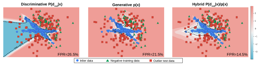
Figure 2: Three anomaly detection approaches on a 2D toy problem. Inliers, train negatives and test anomalies are shown as blue, green and red points. Background heatmap designates the predicted anomaly score $s(\mathbf{x})$ with higher values in red. The discriminative approach (left) is susceptible to false negative responses far from negative training data. The negative dataset is finite and therefore cannot cover all modes of test anomalies. The generative approach (middle) errs along the boundary of the inlier manifold due to over-generalization [27, 29], but is unlikely to commit errors far from the inlier manifold. The hybrid approach attains synergy between discriminative and generative modelling (Sec. 3.1).

3 Hybrid Open-set Segmentation

We propose a dense hybrid anomaly score that incorporates both discriminative and generative cues for anomaly detection (Sec. 3.1). Our score can be efficiently fused with a semantic classifier (Sec. 3.2) in order to produce a dense hybrid open-set model (Sec. 3.3).

We represent input images with a random variable $\underline{\mathbf{x}}$. Categoric random variable $\underline{y}^{ij}$ denotes the label at the location ($i,j$), while the binary random variable $\underline{d}^{ij}$ models whether the given pixel is an inlier or as outlier. We write $d_{\mathrm{in}}^{ij}$ for inliers and $d_{\mathrm{out}}^{ij}$ for outliers. Finally, we denote a realization of a random variable by omitting the underline and often omit spatial locations for brevity. Thus, $P(y^{ij}|\mathbf{x})$ is a shortcut for $P(\underline{y}^{ij}=y^{ij}|\underline{\mathbf{x}}=\mathbf{x})$.

3.1 Hybrid Anomaly Detection

We argue that discriminative and generative anomaly detection exhibit different failure modes (cf. Fig. 2). Discriminative approaches model the dataset posterior $P(d_{\mathrm{in}}|\mathbf{x})$. However, this often fails since a finite negative training dataset cannot cover all modes of the test anomalies. Generative approaches model the data likelihood $p(\mathbf{x})$. These approaches often err along the boundary of the inlier manifold due to over-generalization [27, 29], but do not expand into unlimited open-space as their discriminative counterparts. We fuse the two approaches into a hybrid score that yields high values when both components indicate an anomaly. Our hybrid approach achieves synergy by avoiding both the coarseness of the generative approach and the over-confidence of the discriminative approach. Fig. 2 illustrates the advantages of a hybrid approach on a toy example. Details about the dataset and models are in the Appendix.

Our hybrid anomaly detector builds upon the discriminative dataset posterior $P(d_{\mathrm{in}}|\mathbf{x})$ and the generative data likelihood $p(\mathbf{x})$. We express a general formulation of our hybrid anomaly score $s:\mathcal{X}\rightarrow\mathbb{R}$ as follows:

$$s(\mathbf{x}):=\mathcal{F}(P(d_{\mathrm{out}}|\mathbf{x}),p(\mathbf{x})).$$ (1)

The concrete definition of $\mathcal{F}$ may differ depending on the application. The next subsection formulates the two components atop standard dense prediction and propose a concrete implementation of $\mathcal{F}$.

3.2 Efficient Implementation Atop Semantic Classifier

Standard semantic classification can be viewed as a two-step procedure. Given an input image $\mathbf{x}$, a deep feature extractor $f_{\theta_{1}}$ computes an abstract representation $\mathbf{z}$ also known as pre-logits. Then, the computed pre-logits are projected into logits $\mathbf{s}$ and activated by softmax. The softmax output models the class posterior $P(y|\mathbf{x})$:

$$P(y|\mathbf{x}):=\mathrm{softmax}(\mathbf{s})_{y},\;\text{where}\;\mathbf{s}=f_{\theta_{2}}(\mathbf{z}),\,\mathbf{z}=f_{\theta_{1}}(\mathbf{x}).$$ (2)

In practice, $f_{\theta_{1}}$ can be any dense feature extractor that is suitable for semantic segmentation, while $f_{\theta_{2}}$ is a simple projection by means of 1x1 convolution. We extend this framework with dense data likelihood and discriminative dataset posterior.

Dense data likelihood can be expressed atop the dense classifier $f_{\theta_{2}}$ by re-interpreting logits as unnormalized log-joint density of the input and the label [48]:

$$p(y,\mathbf{x})=\frac{1}{Z}\hat{p}(y,\mathbf{x}):=\frac{1}{Z}\exp{\mathbf{s}_{y}},\;\;\text{where}\;\;\;\mathbf{s}=f_{\theta_{2}}(\mathbf{z}).$$ (3)

$Z$ denotes the corresponding normalization constant dependent only on model parameters. As usual, $Z$ is finite but intractable, since it requires aggregating the unnormalized distribution for all realizations of $\underline{y}$ and $\underline{\mathbf{x}}$: $Z=\int_{\mathbf{x}}\sum_{y}\exp{\mathbf{s}_{y}}$. Throughout this work, we conveniently eschew the evaluation of $Z$ in order to enable efficient training and inference.

We express the dense likelihood $p(\mathbf{x})$ by marginalizing out $\underline{y}$:

$$p(\mathbf{x})=\sum_{y}p(y,\mathbf{x})=\frac{1}{Z}\,\sum_{y}\hat{p}(y,\mathbf{x})=\frac{1}{Z}\,\sum_{y}\exp{\mathbf{s}_{y}}.$$ (4)

Consequently, the unnormalized likelihod is defined as $\hat{p}(\mathbf{x})=\sum_{y}\exp\mathbf{s}_{y}$, where $\mathbf{s}$ represents the logits. The standard discriminative predictions (2) are consistently recovered as $p(y,\mathbf{x})/p(\mathbf{x})$ according to Bayes rule [48]:

$$P(y|\mathbf{x})=\frac{p(y,\mathbf{x})}{\sum_{y^{\prime}}p(y^{\prime},\mathbf{x})}=\frac{\exp{\mathbf{s}_{y}}}{\sum_{y^{\prime}}\exp{\mathbf{s}_{y^{\prime}}}}=\mathrm{softmax}(\mathbf{s})_{y}.$$ (5)

The normalization constant $Z$ appears both in the numerator and denominator, and hence cancels out. Reinterpretation of logits enables convenient unnormalized per-pixel likelihood estimation atop standard semantic segmentation and even exploiting pre-trained classifiers. Note that adding a constant value to the logits does not affect the standard classification but affects our framework since the value of $p(\mathbf{x})$ changes. We exploit the extra degree of freedom in order to express the data likelihood [48] .

We define the dataset posterior $P(d_{\mathrm{in}}|\mathbf{x})$ as a non-linear transformation of pre-logits $\mathbf{z}$ [17]:

$$P(d_{\mathrm{in}}|\mathbf{x}):=\sigma(g_{\gamma}(\mathbf{z})).$$ (6)

We propose to materialize our dense hybrid anomaly score (1) by defining $\mathcal{F}$ as a log ratio:

$$s(\mathbf{x}):=\ln\frac{P(d_{\mathrm{out}}|\mathbf{x})}{p(\mathbf{x})}\cong\ln P(d_{\mathrm{out}}|\mathbf{x})-\ln\hat{p}(\mathbf{x}).$$ (7)

We can neglect $Z$ since ranking performance [37] is invariant to monotonic transformations such as taking a logarithm or adding a constant. The detailed derivation is in the Appendix. Our hybrid anomaly score is a log-ratio of the dataset posterior and unnormalized data likelihood. We propose this particular formulation in order to equalize the influence of the two components. Our score is well suited for dense prediction due to minimal overhead and translation equivariance. Other definitions of $\mathcal{F}$ may also be effective, which is an interesting direction for future work.

3.3 Dense Open-set Inference

The proposed hybrid anomaly detector can be combined with the closed-set output to recover open-set segmentation as shown in Fig. 3. RGB input is fed to a dense feature extractor which produces pre-logits $\mathbf{z}$ and logits $\mathbf{s}$. We activate the closed-set class posterior $P(y|\mathbf{x})$ with softmax and the unnormalized data log-likelihood $\ln\hat{p}(\mathbf{x})$ via log-sum-exp operator (designated in green). A distinct head $g$ transforms pre-logits $\mathbf{z}$ into the dataset posterior $P(d_{\mathrm{in}}|\mathbf{x})$ (designated in yellow). The anomaly score $s(\mathbf{x})$ follows the equation (7). The resulting anomaly map is thresholded and fused with the discriminative output into the final dense open-set recognition map. The desired behaviour of the dense hybrid open-set model is attained by fine-tuning a pre-trained classifier according to the procedure defined in the following section.

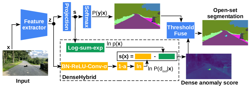
Figure 3: The proposed open-set segmentation approach. Our dense anomaly score is a log-ratio of dataset posterior and data likelihood. Both components can be derived from any semantic segmentation architecture. We implement open-set segmentation by overriding the closed-set segmentation map with the thresholded anomaly score.

4 Open-set Training with DenseHybrid

Our open-set approach complements an arbitrary closed-set segmentation model with the DenseHybrid anomaly detector. We propose a novel training setup that eschews the intractable normalization constant by introducing negative data to the generative learning objective (Sec. 4.1). The same negative data is used to train the dataset posterior. We relax dependence on real negatives by sampling a suitably trained normalizing flow (Sec. 4.2).

4.1 Open-set Training with Real Negative Data

Our hybrid open-set model requires joint fine-tuning of three dense prediction heads: closed-set class posterior $P(y|\mathbf{x})$, unnormalized data likelihood $\hat{p}(\mathbf{x})$ [48], and dataset posterior $P(d_{\mathrm{in}}|\mathbf{x})$ [17]. The corresponding training objectives are presented in the following paragraphs.

Class posterior. The closed-set class-posterior head can be trained according to the standard discriminative cross-entropy loss over the inlier dataset $D_{\mathrm{in}}$:

$$L_{\mathrm{cls}}(\theta) =\mathbb{E}_{\mathbf{x},y\in D_{\mathrm{in}}}[-\ln P(y|\mathbf{x})]$$ (8)

$$=-\,\mathbb{E}_{\mathbf{x},y\in D_{\mathrm{in}}}[\mathbf{s}_{y}-\underset{y^{\prime}}{\text{LSE}}(\mathbf{s}_{y^{\prime}})].$$ (9)

As before, $\mathbf{s}$ are logits computed by $f_{\theta}$, while LSE stands for log-sum-exp operator where the sum iterates over classes.

Data likelihood. Training unnormalized likelihood can be a daunting task since backpropagation through $p(\mathbf{x})$ involves intractable integration over all possible images [67, 68]. Previous solutions are based on MCMC sampling [48], however, this is not feasible in our setup due to high-resolution inputs and dense prediction. We eschew the normalization constant by optimizing the likelihood both in inlier and outlier pixels:

$$L_{\mathbf{x}}(\theta) =\mathbb{E}_{\mathbf{x}\in D_{\mathrm{in}}}[-\ln p(\mathbf{x})]-\mathbb{E}_{\mathbf{x}\in D_{\mathrm{out}}}[-\ln p(\mathbf{x})]$$ (10)

$$=-\mathbb{E}_{\mathbf{x}\in D_{\mathrm{in}}}[\ln\hat{p}(\mathbf{x})]+\mathbb{E}_{\mathbf{x}\in D_{\mathrm{out}}}[\ln\hat{p}(\mathbf{x})]$$ (11)

$$=-\,\mathbb{E}_{D_{\mathrm{in}}}[\underset{i}{\text{LSE}}(\mathbf{s}_{i})]+\,\mathbb{E}_{D_{\mathrm{out}}}[\underset{i}{\text{LSE}}(\mathbf{s}_{i})]$$ (12)

Note that the normalization constant $Z$ cancels out due to training on outliers. Step-by-step loss derivation can be found in the Appendix. In practice, we use a simplified loss that corresponds to an upper bound of the above expression ($L_{\mathbf{x}}^{\mathrm{UB}}\geq L_{\mathbf{x}}$):

$$L_{\mathbf{x}}^{\mathrm{UB}}(\theta)=-\,\mathbb{E}_{\mathbf{x},y\in D_{\mathrm{in}}}[\mathbf{s}_{y}]+\,\mathbb{E}_{\mathbf{x}\in D_{\mathrm{out}}}[\underset{i}{\text{LSE}}(\mathbf{s}_{i})].$$ (13)

Proof can be easily derived by recalling that log-sum-exp is a smooth upper bound of the max function. Thus, our upper bound $L_{\mathbf{x}}^{\mathrm{UB}}$ leverages the following inequalities:

$$\ln\sum_{i}\exp{\mathbf{s}_{i}}\geq\max_{i}\mathbf{s}_{i}\geq\mathbf{s}_{y}.$$ (14)

Recall that training data likelihood only on inliers [67, 48] would require MCMC sampling, which is infeasible in our context. Unnormalized likelihood could also be trained through score matching [68]. However, this would preclude hybrid modelling due to having to train on noisy inputs. Consequently, it appears that the proposed training approach is a method of choice in our context. Comparison of the discriminative loss (9) and the generative upper bound (13) reveals that the standard classification loss is well aligned with the upper bound in inlier pixels.

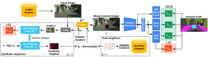
Figure 4: The fine-tuning procedures for the proposed DenseHybrid model. We construct mixed-content images by pasting negatives into inlier images according to (17). The negative training data can be sourced exclusively from an auxiliary real dataset (Sec. 4.1), from a jointly trained normalizing flow (Sec. 4.2), or from both sources according to $b$ from (20). Mixed-content images are fed to the open-set model that produces three dense outputs: the closed-set class posterior, unnormalized data likelihood, and dataset posterior. Outputs are optimized according to the compound loss (16). In the case of synthetic negatives, the normalizing flow optimizes the loss (19).

Dataset posterior. The dataset-posterior head $P(d_{\mathrm{in}}|\mathbf{x})$ requires a discriminative loss that distinguishes the inliers $\mathbf{x}\in D_{\mathrm{in}}$ from the outliers $\mathbf{x}\in D_{\mathrm{out}}$ [17]:

$$L_{\mathbf{d}}(\theta,\gamma)=-\mathbb{E}_{\mathbf{x}\in D_{\mathrm{in}}}[\ln P(d_{\mathrm{in}}|\mathbf{x})]\\ -\mathbb{E}_{\mathbf{x}\in D_{\mathrm{out}}}[\ln(1-P(d_{\mathrm{in}}|\mathbf{x}))].$$ (15)

Compound loss. Our final compound loss aggregates $L_{\mathrm{cls}}$, $L_{\mathbf{x}}^{\mathrm{UB}}$ and $L_{\mathbf{d}}$:

$$L(\theta,\gamma)=-\mathbb{E}_{\mathbf{x},y\in D_{\mathrm{in}}}[\ln P(y|\mathbf{x})+\ln P(d_{\mathrm{in}}|\mathbf{x})]\\ -\mathbb{E}_{\mathbf{x}\in D_{\mathrm{out}}}[\ln(1-P(d_{\mathrm{in}}|\mathbf{x}))-\ln\hat{p}(\mathbf{x})].$$ (16)

In practice, we use a modulation hyperparameter for every loss term. More on the hyperparameters, together with the complete derivation, can be found in the Appendix.

Figure 4 illustrates the proposed procedure for training open-set segmentation models. We prepare mixed-content training images $\mathbf{x}^{\prime}$ by pasting negative patches $\mathbf{x}^{-}\in D_{\mathrm{out}}$ into regular training images $\mathbf{x}^{+}\in D_{\mathrm{in}}$:

$$\mathbf{x}^{\prime}=(\mathbf{1}-\mathbf{m})\cdot\mathbf{x}^{+}+\mathrm{pad}(\mathbf{x}^{-},\mathbf{m}),\quad\mathbf{x}^{-}\in D_{\mathrm{out}}.$$ (17)

The binary mask $\mathbf{m}$ identifies negative pixels within the mixed-content image $\mathbf{x}^{\prime}$. Semantic labels of negative pixels are set to void. The resulting mixed-content image $\mathbf{x}^{\prime}$ is fed to the desired segmentation model that produces pre-logits $\mathbf{z}$ and logits $\mathbf{s}$. We recover the class posterior $P(y|\mathbf{x})$ by activating logits with softmax. We recover the unnormalized log-likelihood $\ln\hat{p}(\mathbf{x})$ by processing logits with log-sum-exp. We recover dataset posterior $P(d_{\mathrm{in}}|\mathbf{x})$ by processing pre-logits with $g_{\gamma}$. The compound training loss $L(\theta,\gamma)$ (16) aggregates the class-discriminative loss $L_{\mathrm{cls}}$ (9), generative loss $L_{\mathbf{x}}^{\text{UB}}$ (13) and dataset-discriminative loss $L_{\mathbf{d}}$ (15).

4.2 Open-set Training with Synthetic Negative Data

Training anomaly detectors on real negative training data may result in over-optimistic performance estimates due to non-empty intersection between the training negatives and test anomalies. This issue can be addressed by replacing real negative training data with samples from a suitable generative model [33, 35, 69, 70]. The generative model can be trained to generate synthetic samples that encompass the inlier distribution [33]. The required learning signal can be derived from discriminative predictions [33, 35, 70] or provided by an adversarial module [42]. Anyway, replacing real negative data with synthetic counterparts requires joint training of the generative model. We choose a normalizing flow [71] for this task due to good distributional coverage and ability to quickly generate samples of varying spatial dimensions [72]. We train the normalizing flow $p_{\zeta}$ according to a weighted sum of two terms.

The data term $L_{\mathrm{mle}}$ corresponds to crop-wide negative log-likelihood of random crops from inlier images $\mathbf{x}^{+}$:

$$L_{\mathrm{mle}}(\zeta)=-\mathbb{E}_{\mathbf{x}^{+}\in D_{\mathrm{in}}}[\ln p_{\zeta}(\text{crop}(\mathbf{x}^{+},\mathbf{m}))].$$ (18)

The crop notation mirrors the pad notation from (17). Random crops vary in spatial resolution. This term aligns the generative distribution with the distribution of the training data. It encourages coverage of the inlier distribution assuming sufficient capacity of the generative model.

The boundary-attraction term $L_{\mathrm{jsd}}$ [72] corresponds to negative Jensen-Shannon divergence between the class-posterior and the uniform distribution in all generated pixels. This term pushes the generative distribution towards the periphery of the inlier distribution where the class posterior should have a high entropy. Note that gradients of this term must propagate through the entire segmentation model in order to reach the normalizing flow. Hence, the flow is penalized when the generated sample yields high softmax confidence. This signal pushes the generative distribution away from high-density regions of the input space [33]. The total loss of the normalizing flow modulates the contribution of the boundary term with the hyperparameter $\lambda$:

$$L(\zeta)=L_{\mathrm{mle}}(\zeta)+\lambda\cdot L_{\mathrm{jsd}}(\zeta;\theta)$$ (19)

Optimization of (19) enforces the generative distribution to encompass all modes of inlier distribution. Note that our normalizing flow can never match the diversity of images from a real dataset such as COCO or ADE20k. It would be unreasonable to expect a generation of a sofa after training on Cityscapes. Still, if the flow succeeds to learn well the boundary of the inlier distribution, then DenseHybrid will be inclined to associate all off-distribution datapoints with low $\hat{p}(\mathbf{x})$ and low $P(d_{\text{in}}|\mathbf{x})$.

Details of the training procedure are again illustrated in Figure 4. We sample the normalizing flow by i) selecting a random spatial resolution (H,W) from a predefined interval, ii) sampling a random latent representation $\mathbf{z}\sim\mathcal{N}(0,\mathrm{I}_{HW})$, and iii) feeding $\mathbf{z}$ to the flow so that $\mathbf{x}^{-}=h_{\zeta}^{-1}(\mathbf{z})$. We again craft a mixed-content image $\mathbf{x}^{\prime}$ by pasting the synthesized negative patch $\mathbf{x}^{-}\sim p_{\zeta}$ into the regular training image $\mathbf{x}^{+}\in D_{\text{in}}$ according to (17), perform the forward pass, determine $L_{\mathrm{cls}}$, $L_{\mathbf{d}}$, $L_{\mathbf{x}}$, and $L_{\mathrm{jsd}}$, and recover the training gradients by backpropagation. We now take the deleted inlier patch $\mathbf{x}^{+}_{\mathbf{s}}$, perform inference with the normalizing flow ($\mathbf{z}=h_{\zeta}(\mathbf{x}^{+}_{\mathbf{s}}$)) and accumulate gradients of $L_{\mathrm{mle}}$ before performing a model-wide parameter update.

We can also source the negative content from a mixture of real and synthetic samples. Then, the amount of data from each source is modulated by hyperparameter $b\in[0,1]$. The probability of sampling a real negative equals $b$, while the probability of sampling a synthetic negative equals $1-b$. Hence, the distribution of mixed negatives $p_{\text{neg}}$ is:

$$p_{\text{neg}}(\mathbf{x}^{-})=b\cdot p_{\text{out}}(\mathbf{x}^{-})+(1-b)\cdot p_{\zeta}(\mathbf{x}^{-}),\;b\in[0,1]$$ (20)

Sampling $p_{\text{neg}}$ proceeds by first choosing the source, which corresponds to sampling a Bernoulli distribution $\mathcal{B}(b)$. Then, the negative is generated by sampling the selected source. Note that we only require a set of i.i.d. datapoints ($D_{\text{out}}$) sampled from $p_{\text{out}}$ without a closed-form definition of $p_{\text{out}}$.

5 Experimental setup

Evaluation of dense anomaly detection and open-set segmentation requires specialized datasets and benchmarks (Sec. 5.1). None of the existing metrics can quantify the gap between open-set and closed-set segmentation performance. We address this need by proposing a novel Open-mIoU metric (Sec. 5.2). The remaining implementation details are described in the Appendix. Our code will be publicly available within the DenseHybrid repository [73] upon acceptance.

5.1 Benchmarks and Datasets

We evaluate performance on benchmarks for dense anomaly detection and open-set segmentation. Fishyscapes [12] considers urban scenarios on a subset of LostAndFound [14] and on Cityscapes validation images with pasted anomalies (FS Static). SegmentMeIfYouCan (SMIYC) [58] collects carefully selected images from the real world and groups them with respect to the anomaly size into AnomalyTrack (large) and ObstacleTrack (small). Moreover, the benchmark includes a selection of images from LostAndFound [14] where the lost objects do not correspond to the Cityscapes taxonomy. Unfortunately, these benchmarks supply only binary labels, which makes them inappropriate for evaluating open-set performance. Hence, we report only anomaly detection performance on these benchmarks.

We validate performance on Cityscapes while reinterpreting a subset of ignore classes as the unknown class [19]. StreetHazards [74] is a synthetic dataset created with the CARLA virtual environment that enables smooth anomaly injection and low-cost label extraction. Consequently, the dataset contains K+1 labels, making it suitable for measuring open-set recognition performance.

We also validate open-set segmentation on COCO val after training on images from augmented VOC 2012 [75]. There is a 1:1 relationship between the VOC taxonomy and the corresponding 20 COCO classes, although there is a notable covariate shift between the two datasets. The remaining 113 COCO classes are treated as unknowns.

5.2 Measuring open-set performance

Previous work evaluates open-set segmentation through anomaly detection [14, 58] and closed-set segmentation [12]. The observed drop in closed-set performance is usually negligible and is explained by the allocation of model capacity for anomaly detection. However, we will show that the impact of anomalies onto segmentation performance can be clearly characterized only in the open-set setup. More precisely, we shall take into account false positive semantic predictions at anomalies as well as false negative semantic predictions due to false anomaly detections.

We propose a novel evaluation procedure for open-set segmentation. Our procedure starts by thresholding the anomaly score so that it yields 95% TPR anomaly detection on held-out data. Then, we override the classification in pixels which score higher than the threshold. This yields a recognition map with $K+1$ labels. We assess open-set segmentation performance according to a novel metric that we term open-mIoU. We compute open-IoU for the $k$-th class as follows:

$$\text{open-IoU}_{k}=\frac{\mathrm{TP}_{k}}{\mathrm{TP}_{k}+\mathrm{FP}^{\text{os}}_{k}+\mathrm{FN}^{\text{os}}_{k}},\quad\mathrm{where}$$ (21)

$$\mathrm{FP}^{\text{os}}_{k}=\sum_{i=1,i\neq k}^{K+1}\mathrm{FP}_{k}^{i},\quad\mathrm{FN}^{\text{os}}_{k}=\sum_{i=1,i\neq k}^{K+1}\mathrm{FN}_{k}^{i}.$$ (22)

Different than the standard IoU formulation, open-IoU takes into account false predictions due to imperfect anomaly detection. In particular, a prediction of class $k$ at an outlier pixel (false negative anomaly detection) counts as a false positive for class $k$. Furthermore, a prediction of class K+1 at a pixel labelled as class $k$ (false positive anomaly detection) counts as a false negative for class $k$. Note that we still average open-IoU over $K$ inlier classes. Thus, a recognition model with perfect anomaly detection gets assigned the same performance as in the closed world. This property would not be preserved if we averaged open-IoU over K+1 classes. Hence, a comparison between mIoU and open-mIoU quantifies the gap between the closed-set and open-set performance, unlike any of the related metrics such as m$F_{1}$ [59, 19].

TABLE I: Anomaly detection performance on SegmentMeIfYouCan [58] and Fishyscapes [20]. Aux data denotes training on real negatives, while Img rsyn. denotes image resynthesis.

Method			SegmentMeIfYouCan [58]						Fishyscapes [12]
	Aux	Img	AnomalyTrack		ObstacleTrack		LAF-noKnown		FS LAF		FS Static		CS val
	data	rsyn.	AP	$\mathrm{FPR}_{95}$	AP	$\mathrm{FPR}_{95}$	AP	$\mathrm{FPR}_{95}$	AP	$\mathrm{FPR}_{95}$	AP	$\mathrm{FPR}_{95}$	$\overline{\mathrm{IoU}}$
Image Resyn. [22]	✗	✓	52.3	25.9	37.7	4.7	57.1	8.8	5.7	48.1	29.6	27.1	81.4
Road Inpaint. [76]	✗	✓	-	-	54.1	47.1	82.9	35.8	-	-	-	-	-
Max softmax [37]	✗	✗	28.0	72.1	15.7	16.6	30.1	33.2	1.8	44.9	12.9	39.8	80.3
MC Dropout [26]	✗	✗	28.9	69.5	4.9	50.3	36.8	35.6	-	-	-	-	-
ODIN [38]	✗	✗	33.1	71.7	22.1	15.3	52.9	30.0	-	-	-	-	-
SML [77]	✗	✗	-	-	-	-	-	-	31.7	21.9	52.1	20.5	-
Embed. Dens. [12]	✗	✗	37.5	70.8	0.8	46.4	61.7	10.4	4.3	47.2	62.1	17.4	80.3
JSRNet [24]	✗	✗	33.6	43.9	28.1	28.9	74.2	6.6	-	-	-	-	-
SynDenseHybrid (ours)	✗	✗	51.5	33.2	64.0	0.6	78.8	1.1	51.8	11.5	54.7	15.5	79.9
SynBoost [23]	✓	✓	56.4	61.9	71.3	3.2	81.7	4.6	43.2	15.8	72.6	18.8	81.4
Prior Entropy [78]	✓	✗	-	-	-	-	-	-	34.3	47.4	31.3	84.6	70.5
OOD Head [45]	✓	✗	-	-	-	-	-	-	31.3	19.0	96.8	0.3	79.6
Void Classifier [12]	✓	✗	36.6	63.5	10.4	41.5	4.8	47.0	10.3	22.1	45.0	19.4	70.4
Dirichlet prior [78]	✓	✗	-	-	-	-	-	-	34.3	47.4	84.6	30.0	70.5
DenseHybrid (ours)	✓	✗	78.0	9.8	87.1	0.2	78.7	2.1	43.9	6.2	72.3	5.5	81.0

Figure 5 compares the considered closed-set (top left, $\text{IoU}_{k}$) and open-set (right, $\text{open-IoU}_{k}$) metrics. Imperfect anomaly detection impacts recognition performance through increased false positive (designated in yellow) and false negative semantics (designated in red). Difference between closed-set mIoU and open-mIoU reveals the performance gap due to inaccurate anomaly detection.

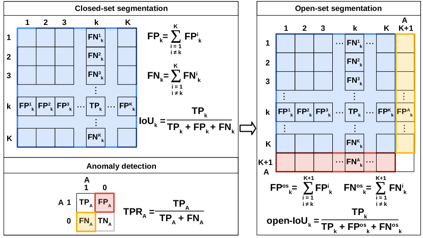
Figure 5: We extend closed-set performance evaluation (top-left) with a novel open-set metric (right). Open-IoU takes into account false positive semantics at undetected anomalies as well as false negative semantics due to false positive anomalies. The proposed open-mIoU metric quantifies recognition performance in presence of anomalies.

6 Experimental results

We evaluate DenseHybrid performance in dense anomaly detection (Sec. 6.1) and open-set segmentation (Sec. 6.2, 6.3) after training with and without real negative data. We also ablate various components of our method (Sec. 6.4, 6.5). Practical aspects of our method (e.g. inference speed and distance-wise performance) can be found in the Appendix.

6.1 Dense Anomaly Detection in Open-set Setups

Table I presents dense anomaly detection performance on SMIYC [58] and Fishyscapes [20]. We include our model trained on real negative data (DenseHybrid) and on synthetic negatives (SynDenseHybrid). DenseHybrid outperforms contemporary approaches on both AnomalyTrack and ObstacleTrack by a wide margin. Also, it achieves the best $\mathrm{FPR}_{95}$ on LostAndFound-noKnown. Similarly, it delivers the best performance on Fishyscapes LostAndFound and the best $\mathrm{FPR}_{95}$ on Static.

SynDenseHybrid outperforms all previous methods that do not train on real negative data on ObstacleTrack and LostAndFound-noKnown. In the case of AnomalyTrack, it is outperformed only by image resynthesis [22] that requires significant computational overhead. Also, SynDenseHybrid achieves the best performance on all but one metric of Fishyscapes and the second-best AP on Fishyscapes Static. As in the case of training on real negative data, the hybrid anomaly detector achieves the best performance on Fishyscapes with exception of AP on Static. All our performance estimates use standard performance metrics of the particular datasets. Our performance metrics on Fishyscapes LostAndFound would increase if we considered only the road pixels as in [24]. The rightmost column of the table indicates that our fine-tuning protocol exerts a negligible impact on closed-set performance. However, the next section will show that the impact of anomaly detection on final recognition performance is more significant than what can be measured with closed-set metrics.

Figure 6 shows synthetic negatives produced by the training setup from Sec. 4.2. Samples vary in spatial resolution and lack meaningful visual concepts. Yet, training our open-set model on such samples yields only slightly worse performance than when training on real negative data.

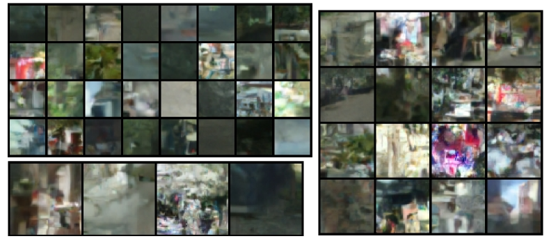
Figure 6: Synthetic negatives sampled from our normalizing flow (cf. Sec. 4.2). These samples are pasted into training crops instead of real negatives (instances from ADE20k). We sample the normalizing flow at different resolutions to mimic real-world anomalies which vary in size.

Table II presents performance on Road Anomaly[22] and validation subsets of Fishyscapes. The top section presents methods which do not train on real negative data. The bottom section presents methods which train on real negative data. Our method performs competitively with respect to the previous work in both setups.

TABLE II: Performance of DenseHybrid on Road Anomaly and Fishyscapes val.

Model	RA		FS L&F		FS Static
	AP	$\mathrm{FPR}$	AP	$\mathrm{FPR}$	AP	FPR
MSP [37]	15.7	71.4	4.6	40.6	19.1	24.0
ML [74]	19.0	70.5	14.6	42.2	38.6	18.3
SML [77]	25.8	49.7	36.6	14.5	48.7	16.8
SynthCP [46]	24.9	64.7	6.5	46.0	23.2	34.0
Emb. Density [12]	-	-	4.1	22.3	-	-
SynDenseHybrid	35.1	37.2	60.2	7.9	52.1	7.7
SynBoost[23]	38.2	64.8	60.6	31.0	66.4	25.6
OOD head [17]	-	-	45.7	24.0	-	-
Energy [41]	19.5	70.2	16.1	41.8	41.7	17.8
DenseHybrid	63.9	43.2	60.5	6.0	63.1	4.2

We also validate our method by considering a subset of Cityscapes void classes as the unknown class. More precisely, we consider all void classes except ’unlabeled’, ’ego vehicle’, ’rectification border’, ’out of roi’ and ’license plate’ as unknowns during validation [19]. Table III compares performance according to the AUROC (AUC) metric. SynDenseHybrid outperforms all previous works. Most notably, it outperforms the previous SotA [19] by four percentage points. To offer fair comparison with previous work, we do not report results when training on real negative data.

TABLE III: Open-set segmentation performance on Cityscapes val. Following [19], we consider a subset of ignore classes as unknowns.

Method	AUC	Method	AUC
MSP [37]	72.1	GDM [79]	74.3
Entropy [80]	69.7	GMM [69]	76.5
OpenMax [53]	75.1	K+1 classifier	75.5
C2AE [81]	72.7	OpenGAN-O [19]	70.9
ODIN [38]	75.5	OpenGAN [19]	88.5
MC dropout [26]	76.7	SynDenseHybrid (ours)	92.9

6.2 Open-set Segmentation

We consider open-set performance according to mean $F_{1}$ ($\overline{F_{1}}$) score and the proposed open-mIoU (o$\overline{\mathrm{IoU}}$) metric. Table IV presents performance evaluation on StreetHazards. The left part of the table considers anomaly detection while the right part considers closed-set and open-set segmentation performance. Our method outperforms contemporary approaches in anomaly detection both with and without training on real negative data. Furthermore, our method achieves the best open-set performance (columns o$\overline{\mathrm{IoU}}$ and $\overline{F_{1}}$) despite lower closed-set segmentation score ($\overline{\mathrm{IoU}}$ column). The performance gap between closed-set and open-set can be quantified as the difference between $\overline{\mathrm{IoU}}$ and o$\overline{\mathrm{IoU}}$ (”Gap” column). Our method achieves the least performance gap of around 18 percentage points. Nevertheless, an ideal anomaly detector would deliver equal open-set and closed-set metrics. Hence, we conclude that even the state-of-the-art anomaly detectors are still incapable to deliver closed-set performance in open-set setups. Researchers should strive to diminish this gap in order to improve the safety of recognition systems in the real world.

TABLE IV: Performance evaluation on StreetHazards [74]. We evaluate anomaly detection (Anomaly), closed-set segmentation (Cls.), open-set segmentation (Open-set), and the open-set performance gap (Gap).

Method	Anomaly			Cls.	Open-set		Gap
	AP	$\mathrm{FPR}$	AUC	$\overline{\mathrm{IoU}}$	$\overline{\mathrm{F_{1}}}$	o$\overline{\mathrm{IoU}}$
SynthCP [46]	9.3	28.4	88.5	-	-	-	-
Dropout [26]	7.5	79.4	69.9	-	-	-	-
TRADI [82]	7.2	25.3	89.2	-	-	-	-
SO+H [35]	12.7	25.2	91.7	59.7	-	-	-
DML [18]	14.7	17.3	93.7	-	-	-	-
MSP [37]	7.5	27.9	90.1	65.0	46.4	35.1	29.9
ODIN [38]	7.0	28.7	90.0	65.0	41.6	28.8	36.2
ReAct [83]	10.9	21.2	92.3	62.7	46.4	34.0	28.7
SynDnsHyb	19.7	17.4	93.9	61.3	50.6	37.3	24.0
Energy [41]	12.9	18.2	93.0	63.3	50.4	42.7	29.9
OE [32]	14.6	17.7	94.0	61.7	56.1	43.8	17.9
OH [45]	19.7	56.2	88.8	66.6	-	33.9	32.7
OH*MSP [17]	18.8	30.9	89.7	66.6	-	43.6	23.0
DenseHybrid	30.2	13.0	95.6	63.0	59.7	45.8	17.2

Figure 7 visualizes qualitative open-set segmentation performance on StreetHazards test. Our hybrid anomaly detector accurately combines dense anomaly detection (second row) with closed-set segmentation and delivers open-set segmentation (third row). Contemporary energy-based approach [41] yields more false positives (fourth row).

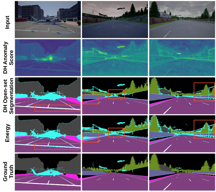
Figure 7: Qualitative open-set segmentation performance on StreetHazards. DenseHybrid (rows 2 and 3) delivers a more accurate open-set performance with respect to the energy-based approach [41] (row 4), as denoted with red rectangles. Zoom in for a better view.

6.3 Open-set Segmentation under Covariate Shift

Table V presents open-set segmentation performance on 5k crowdsourced photos from the Pascal-COCO benchmark. We train Segmenter [8] with ViT-L/16 backbone on 1464 + 11355 images from augmented Pascal VOC. During training, we set all background VOC pixels to the mean pixel to prevent leakage of anomalous semantic content to the inlier representations. Our hybrid open-set method outperforms previous approaches when training with real negatives from ADE20K [32, 41] as well as with synthetic negatives [74, 54, 38]. Interestingly, the closed-set model reaches more than 80% mIoU but open-IoU peaks at 36%. Analysis of false positives reveals that the task is hard due to covariate shift between train and test datasets - the known classes contain variable concepts (e.g. different species of potted plants). Moreover, some unknown classes have similar appearance to known classes (eg. unknown zebra and known horse). Finally, the benchmark has high openness [51] - there are $5\times$ more unknown than known classes.

TABLE V: Open-set segmentation on Pascal VOC - COCO.

Model	Aux.	AP	AUC	FPR	$\overline{F_{1}}$	$\overline{\text{oIoU}}$
Max-logit [74, 54]	✗	92.6	78.9	70.4	7.3	6.0
ODIN [38]	✗	90.4	74.3	74.6	6.8	5.6
SynDenseHybrid	✗	93.3	81.0	63.0	13.4	10.6
Energy [41]	✓	94.5	83.6	57.6	14.5	11.9
OE [32]	✓	95.1	85.5	51.9	22.7	18.0
DenseHybrid	✓	96.3	88.5	45.2	48.9	36.2

Figure 8 shows qualitative examples of open-set segmentation on COCO. Our hybrid open-set model correctly identifies known objects in the scene as well as unknown pixels (third column, colored in cyan). The semantic predictions are rather coarse due to ViT backbone patch size. More qualitative examples can be found in the Appendix.

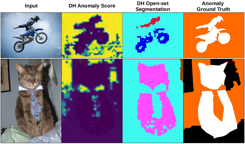
Figure 8: Qualitative open-set segmentation performance on COCO. Unknown pixels are shown in cyan (third column) and correspond well with the ground truth (fourth column, unknown pixels colored in orange).

6.4 Ablating Components of DenseHybrid

Table VI validates components of our hybrid anomaly detection approach on Fishyscapes val. The top two sections compare our hybrid anomaly detector (7) with its generative and discriminative components – $\hat{p}(\mathbf{x})$ and $P(d_{\mathrm{in}}|\mathbf{x})$ – when training on real and synthetic negative data, respectively. We observe that the hybrid detector outperforms unnormalized density which outperforms dataset posterior. We observe the same qualitative behaviour when training on real and synthetic negative data. Bottom section replaces our unnormalized likelihood with likelihood of pre-logits as estimated by a normalizing flow. The flow is applied point-wise to obtain dense likelihood, similar to embeding density [12]. This can also be viewed as a generalization of a previous image-wide open-set approach [44] to dense prediction. We still train on negative data in an end-to-end fashion in order to make the two generative components comparable. The resulting model delivers good performance on FS Static and poor performance on FS LostAndFound. We attribute better performance of our unnormalized density (4) with respect to point-wise flow on FS LostAndFound due to 4$\times$ subsampling of the pre-logits to which the flow is fitted.

TABLE VI: Validation of hybrid anomaly detection on Fishyscapes val. Hybrid formulation outperforms its generative and discriminative components.

Anomaly detector	Neg.	FS L&F		FS Static
	data	AP	$\mathrm{FPR}$	AP	$\mathrm{FPR}$
Disc. $(1-P(d_{\mathrm{in}}|\mathbf{x}))$		46.5	38.3	53.5	30.9
Gen. $\hat{p}(\mathbf{x})=\text{LSE}(\mathbf{s})$	Real	58.2	7.3	58.0	5.3
Hyb. $(1-P(d_{\mathrm{in}}|\mathbf{x}))/\hat{p}(\mathbf{x})$		60.5	6.0	63.1	4.2
Disc. $(1-P(d_{\mathrm{in}}|\mathbf{x}))$		30.1	35.0	48.8	39.8
Gen. $\hat{p}(\mathbf{x})=\text{LSE}(\mathbf{s})$	Syn.	58.1	9.0	44.6	9.5
Hyb. $(1-P(d_{\mathrm{in}}|\mathbf{x}))/\hat{p}(\mathbf{x})$		60.2	7.9	52.1	7.7
Gen. flow $p(\mathbf{z})$	Real	5.7	58.9	61.7	7.6
Hyb. $(1-P(d_{\mathrm{in}}|\mathbf{x}))/p(\mathbf{z})$		6.5	46.1	65.1	6.5

Table VII presents the performance of our hybrid open-set model depending on the source of synthetic negative data. We compare the negatives sampled from normalizing flow with patches of uniform noise, local adversarial attacks [42], inlier crops [24] as well as negatives generated by GAN [33, 19]. We observe that our hybrid model delivers promising performance with different sources of negative content. Further 1-on-1 comparison shows that our normalizing flow provides the most consistent performance.

TABLE VII: Hybrid model performance with different kinds of synthetic negatives.

Source of	FS L&F		FS Static
negatives	AP	FPR	AP	FPR
Uniform noise	56.9	9.2	37.4	9.8
Inlier crops [24]	64.3	8.7	36.2	10.4
GAN [33]	58.7	7.5	34.4	15.2
Loc. Adv. Attacks [42]	44.5	8.8	36.8	11.8
Jointly trained NFlow (ours)	60.2	7.9	52.1	7.7

6.5 Mixing Real and Synthetic Negative Data

Figure 9 shows anomaly detection performance when mixing real negatives from ADE20k and synthetic negatives generated by our normalizing flow. The negative data is mixed according to the hyperparameter $b$ as described in Sec. 4.2. Natural scenes prefer training on mixed negative data (FS L&F) while scenes with synthetically injected anomalies prefer real negative data (FS Static). Hence, open-set training with a mixture of real and synthetic negatives might be beneficial. Results are averaged over five runs.

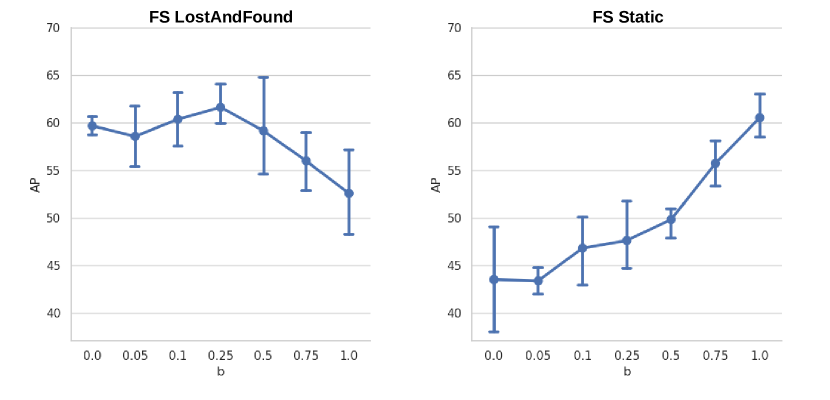
Figure 9: Performance of our hybrid anomaly detector when training on mixtures of $b$ real and $1-b$ synthetic negatives for $b\in[0,1]$.

7 Conclusion

Discriminative and generative approaches to anomaly detection assume different failure modes. We achieve synergy between these two approaches by fusing dataset posterior with unnormalized data likelihood. We refer to the resulting method as DenseHybrid since its low computational overhead and translational equivariance are especially well suited for dense prediction context. DenseHybrid eschews the evaluation of the intractable normalization constant by leveraging negative training data. The negative data can be sourced from a general-purpose dataset, generated by a jointly trained normalizing flow, or correspond to a mixture of both sources. DenseHybrid can be attached to closed-set segmentation approaches in order to attain open-set competence. We observe competitive performance on the standard benchmarks for dense anomaly detection and open-set segmentation. Furthermore, we propose open-mIoU, a novel metric for evaluating open-set segmentation performance and quantifying the performance gap between closed-set and open-set setups. Suitable directions for future work include extensions towards open-set panoptics, integration with semantic segmentation approaches based on class prototypes [84] and mask-level recognition [85], and further reduction of the performance gap between closed-set and open-set recognition.

Matej Grcić received a M.Sc. degree from the Faculty of Electrical Engineering and Computing in Zagreb. He finished the master study program in Computer Science in 2020. He is pursuing his Ph.D. degree at University of Zagreb, FER. His research interests include generative modeling and open-world recognition.

Siniša Šegvić received a Ph.D. degree in computer science from the University of Zagreb, Croatia. He was a post-doctoral researcher at IRISA Rennes and also at TU Graz. He is currently a full professor at Uni-ZG FER. His research interests focus on deep convolutional architectures for classification and dense prediction.

Hybrid Open-set Segmentation
with Synthetic Negative Data - Appendix

Limitations

It may seem that our method can generate samples due to likelihood evaluation being a standard feature of generative models (except GANs). However, sample generation with unnormalized distributions requires MCMC sampling which is not easily performed at large resolutions and dense loss, at least not with known techniques. Still, our hybrid open-set model delivers competitive performance even without the ability to generate samples. Also, variety and quality of synthetic samples are limited by the capacity of the generative model, which will be mitigated with advances in GPU design.

Extended Derivations

Hybrid Anomaly score. We present a step-by-step derivation of Eq. (7) as follows:

$$s(\mathbf{x}) :=\ln\frac{P(d_{\mathrm{out}}|\mathbf{x})}{p(\mathbf{x})}$$ (23)

$$=\ln\frac{P(d_{\mathrm{out}}|\mathbf{x})}{\hat{p}(\mathbf{x})/Z}$$ (24)

$$=\ln P(d_{\mathrm{out}}|\mathbf{x})-\ln\hat{p}(\mathbf{x})+\ln Z$$ (25)

$$\cong\ln P(d_{\mathrm{out}}|\mathbf{x})-\ln\hat{p}(\mathbf{x}).$$ (26)

Loss for data likelihood. We present a step-by-step derivation of Eq. (12) as follows. Note that normalization constant Z cancels out.

$$L_{\mathbf{x}}(\theta) =\mathbb{E}_{\mathbf{x}\in D_{\mathrm{in}}}[-\ln p(\mathbf{x})]-\mathbb{E}_{\mathbf{x}\in D_{\mathrm{out}}}[-\ln p(\mathbf{x})]$$ (27)

$$=-\mathbb{E}_{\mathbf{x}\in D_{\mathrm{in}}}[\ln\hat{p}(\mathbf{x})-\ln{Z}]-\mathbb{E}_{\mathbf{x}\in D_{\mathrm{out}}}[-\ln\hat{p}(\mathbf{x})-\ln{Z}]$$ (28)

$$=-\mathbb{E}_{\mathbf{x}\in D_{\mathrm{in}}}[\ln\hat{p}(\mathbf{x})]-\ln{Z}+\mathbb{E}_{\mathbf{x}\in D_{\mathrm{out}}}[\ln\hat{p}(\mathbf{x})]+\ln{Z}$$ (29)

$$=-\mathbb{E}_{\mathbf{x}\in D_{\mathrm{in}}}[\ln\hat{p}(\mathbf{x})]+\mathbb{E}_{\mathbf{x}\in D_{\mathrm{out}}}[\ln\hat{p}(\mathbf{x})]$$ (30)

$$=-\,\mathbb{E}_{D_{\mathrm{in}}}[\underset{i}{\text{LSE}}(\mathbf{s}_{i})]+\,\mathbb{E}_{D_{\mathrm{out}}}[\underset{i}{\text{LSE}}(\mathbf{s}_{i})]$$ (31)

Compound loss. We present a step-by-step derivation of Eq. (16) as follows. Recall that $L_{\text{cls}}$ equals to:

$$L_{\mathrm{cls}}(\theta)=-\,\mathbb{E}_{\mathbf{x},y\in D_{\mathrm{in}}}[\mathbf{s}_{y}]+\mathbb{E}_{\mathbf{x},y\in D_{\mathrm{in}}}[\underset{y^{\prime}}{\text{LSE}}(\mathbf{s}_{y}^{\prime})]$$ (32)

Moreover, $L_{\textbf{cls}}^{\text{UB}}$ equals to:

$$L_{\mathbf{x}}^{\mathrm{UB}}(\theta)=-\,\mathbb{E}_{\mathbf{x},y\in D_{\mathrm{in}}}[\mathbf{s}_{y}]+\mathbb{E}_{\mathbf{x}\in D_{\mathrm{out}}}[\underset{i}{\text{LSE}}(\mathbf{s}_{i})].$$ (33)

The two losses have a term in common. Consequently, we can omit one of them in the joint loss:

$$L_{\mathrm{cls}}(\theta)+L_{\mathbf{x}}^{\mathrm{UB}}(\theta)=\\ -\,\mathbb{E}_{\mathbf{x},y\in D_{\mathrm{in}}}[\mathbf{s}_{y}]+\mathbb{E}_{\mathbf{x},y\in D_{\mathrm{in}}}[\underset{y^{\prime}}{\text{LSE}}(\mathbf{s}_{y}^{\prime})]+\mathbb{E}_{\mathbf{x}\in D_{\mathrm{out}}}[\underset{i}{\text{LSE}}(\mathbf{s}_{i})].$$ (34)

The above expression equals to:

$$L_{\mathrm{cls}}(\theta)+L_{\mathbf{x}}^{\mathrm{UB}}(\theta)=-\mathbb{E}_{\mathbf{x},y\in D_{\mathrm{in}}}[\ln P(y|\mathbf{x})]-\mathbb{E}_{\mathbf{x}\in D_{\mathrm{out}}}[\ln\hat{p}(\mathbf{x})]$$ (35)

By further adding the data posterior loss and grouping terms according to the expectations we obtain:

$$L(\theta,\gamma) =L_{\text{cls}}(\theta)+L_{\mathbf{x}}^{\text{UB}}(\theta)+L_{\mathbf{d}}(\theta,\gamma)$$ (36)

$$=-\mathbb{E}_{\mathbf{x},y\in D_{\mathrm{in}}}[\ln P(y|\mathbf{x})+\ln P(d_{\mathrm{in}}|\mathbf{x})]$$ (37)

$$-\mathbb{E}_{\mathbf{x}\in D_{\mathrm{out}}}[\ln(1-P(d_{\mathrm{in}}|\mathbf{x}))-\ln\hat{p}(\mathbf{x})].$$ (38)

In practice, we introduce loss modulation hyperparameters which control the impact of each loss term (cf. Implementation details).

2D Toy Example Details

We generate inlier datapoints by sampling the gaussian mixture $p_{\text{in}}(\mathbf{x})=0.5\cdot\mathcal{N}(\mu_{1},\Sigma_{1})+0.5\cdot\mathcal{N}(\mu_{2},\Sigma_{2})$, where $\mu_{1}=\mu_{2}=0$ and $\Sigma_{1}=\begin{bmatrix}0.9&0\\ 0&0.1\end{bmatrix}$ $\Sigma_{2}=\begin{bmatrix}0.071&0.071\\ -0.639&0.639\end{bmatrix}$. The majority of negative training data is located in the first and fourth quadrants of the considered space to imitate the finite negative datasets. Outlier test data encompass the inlier distribution. The discriminative anomaly detector is a binary classifier which consists of 4 MLP layers hidden layers and ReLU activations. The generative anomaly detector is an energy-based model with similar architecture as the binary classifier. The hybrid anomaly detector combines generative and discriminative detector according to the equation (7). Note that all three anomaly scores are invariant to monotonic transformations hence we can put all three scores at the same scale for visualization purposes. To ensure reproducibility, all samples are generated with a fixed seed which equals 7. Different seeds also yield similar results. Source code for this experiment will be available at the official DenseHybrid repository [73].

Implementation details

We construct our open-set models by starting from any closed-set semantic segmentation model that trains with pixel-level cross-entropy loss. We implement the dataset posterior branch $g_{\gamma}$ as a trainable BN-ReLU-Conv1x1 module. We obtain unnormalized likelihood as the sum of exponentiated logits. We fine-tune the resulting open-set models on mixed-content images with pasted negative ADE20k instances (cf. Sec. 4.1) or synthetic negative patches (cf. Sec. 4.2). In the case of SMIYC, we fine-tune LDN-121 [86] for 10 epochs on images from Cityscapes [87], Vistas [88] and Wilddash2 [57]. In the case of Fishyscapes, we use DeepLabV3+ with WideResNet38 [89]. We fine-tune the model for 10 epochs on Cityscapes. In the case of StreetHazards, we train LDN-121 for 120 epochs in the closed-world setting and then fine-tune the open-set model on mixed-content images. In the case of Pascal-COCO setup we train Segmenter with ViT-L/16 for 50 epochs in inlier data and then fine-tune the model for 5 epochs using mixed-content images. During training, we set all background VOC pixels to the mean pixel value. This prevents leakage of anomalous semantic content to the inlier representations and hence ensures unbiased performance estimates. We optimize the loss (38) with the following hyperparameters:

$$L(\theta,\gamma) =-\mathbb{E}_{\mathbf{x},y\in D_{\mathrm{in}}}[\beta_{1}\cdot\ln P(y|\mathbf{x})+\beta_{2}\cdot\ln P(d_{\mathrm{in}}|\mathbf{x})]$$ (39)

$$-\mathbb{E}_{\mathbf{x}\in D_{\mathrm{out}}}[\beta_{3}\cdot\ln(1-P(d_{\mathrm{in}}|\mathbf{x}))-\beta_{4}\cdot\ln\hat{p}(\mathbf{x})].$$ (40)

$\beta_{1}$ always equals 1. For traffic experiments with LDN-121 $\beta_{2}=\beta_{3}=0.3$ and $\beta_{4}=0.03$. For DLV3+ on traffic scenes $\beta_{2}=\beta_{3}=0.1$ and $\beta_{4}=0.01$ except for Tbl. III where $\beta_{2}=\beta_{3}=1.5$ and $\beta_{4}=0.15$. In the case of Pascal-COCO setup, $\beta_{2}=\beta_{3}=1$ and $\beta_{4}=0.1$ for real and $\beta_{2}=\beta_{3}=0.15$ and $\beta_{4}=0.015$ for synthetic data. Hyperparameter $\lambda$ from (19) always equals 0.03. Configurations that do not rely on real negative data leverage synthetic data of varying resolution as generated by DenseFlow-45-6 [71]. All such experiments pre-train DenseFlow with the standard MLE loss on $64\times 64$ crops from road-driving images (except for Pascal-COCO where we pre-train the flow on Pascal images) prior to joint learning. Our joint fine-tuning experiments last less than 24h on RTX A5000 GPU.

Open-set evaluation on StreetHazards is conducted as follows. We partition the test subset into two folds which correspond to the two test cities - t5 and t6. We set the anomaly score threshold in order to obtain 95% TPR on t5, and measure open-mIoU on t6. Subsequently, we switch the folds and measure open-mIoU on t5. We compute the overall open-mIoU by weighting these two measurements according to the number of images in the two folds.

We implemented [41, 83, 32] into our code base by following publicly available implementations. For the energy fine-tuning [41], we found that the optimal hyperparameters for dense setup are $m_{in}=-15$ and $m_{out}=-5$. ReAct [83] delivers the best results when the method-specific hyperparameter c = 0.99.

On Advantages of Hybrid Formulation

Figure 10 shows examples of synergy between generative and discriminative components attained by our hybrid formulation. The first column shows a situation where the generative component detects anomalous content while the discriminative component yields a false negative response. The second column shows an example where the generative component corrects the false positive response generated by the discriminative component. Finally, the third column shows an example where the discriminative component alleviates a false positive response of the generative component. The presented anomaly maps are produced by a model trained on synthetic negatives generated by our normalizing flow.

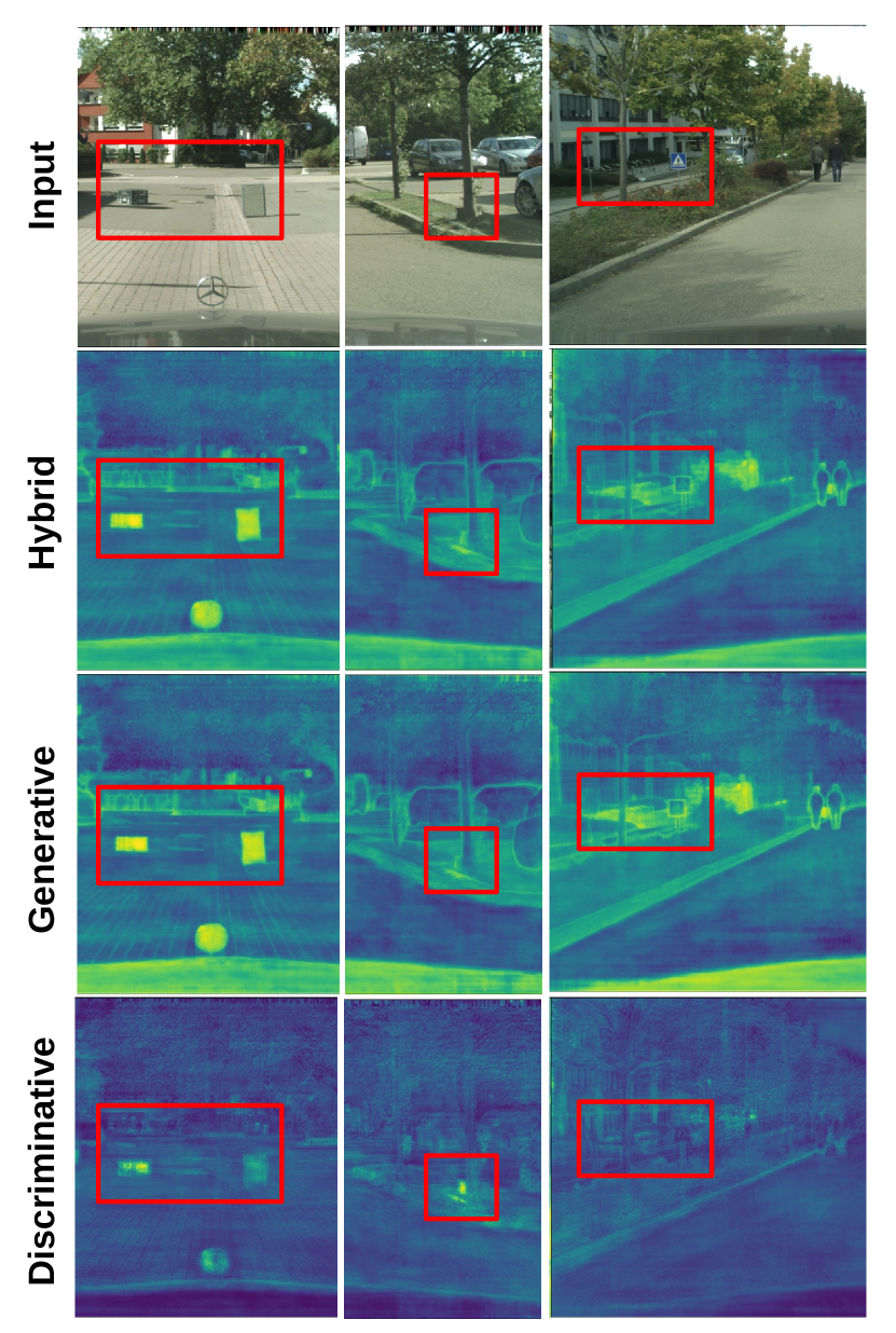
Figure 10: Examples of synergy achieved by fusing the generative and discriminative anomaly detector into a hybrid anomaly detector.

Impact of the Segmentation Model

Table VIII analyzes the impact of different segmentation models upon which we build our open-set approach. The top part of the table shows the standard fully convolutional dense classifier DeepLabV3+ [89] and a convolutional model with near real-time inference LDN-121 [86]. The bottom part shows transformer-based architectures for semantic segmentation Segmenter [8] and SWIN + UpperNet [2]. We see that the final open-set performance indeed depends on the segmentation model. While the convolutional DLV3+ model achieves the best results on FS L&F, the attention-based Segmenter achieves the best results on FS Static. Hence, DenseHybrid can work well with both convolutional and attention-based models.

TABLE VIII: Impact of different segmentation models on DenseHybrid.

Backbone	Upsample	FS L&F		FS Static
		AP	FPR	AP	FPR
WResNet38	DeepLabV3+ [89]	60.5	6.0	63.1	4.2
DenseNet-121	Ladder [86]	20.9	46.2	85.8	4.1
SWIN-B	UpperNet [2]	17.7	59.3	91.3	1.6
ViT-L/16	Segmenter [8]	38.3	24.4	93.6	0.5

Impact of the Depth to the Detection Performance

Road driving scenes typically involve a wide range of depth. Hence, we explore the anomaly detection performance at different ranges from the camera in order to gain a better insight into the performance of different methods. We perform these experiments on LostAndFound test [14] since it provides information about the depth in each ground pixel. Due to errors in the provided disparity maps, we perform our analysis up to 50 meters from the camera. Table IX indicates that DenseHybrid achieves accurate results even at large distances from the vehicle. We observe that SynBoost [23] is better than our approach at the shortest range. However, the computational complexity of image resynthesis precludes real-time deployment of such approaches [23, 22, 46] on present hardware as we show next.

TABLE IX: Anomaly detection performance at different distances from camera.

Range	MSP [37]		ML [74]		SynBoost [23]		DH (ours)
	AP	FPR	AP	FPR	AP	FPR	AP	FPR
5-10	28.7	16.4	76.1	5.4	93.7	0.2	90.7	0.3
10-15	28.8	29.7	73.9	16.2	78.7	17.7	89.8	1.1
15-20	26.0	28.8	78.2	5.9	76.9	25.0	92.9	0.6
20-25	25.1	44.2	69.6	12.8	70.0	23.3	89.1	1.4
25-30	29.0	41.3	72.6	9.5	65.6	18.8	89.5	1.4
30-35	26.2	47.8	70.2	10.0	58.5	27.4	87.7	2.5
35-40	29.6	44.7	71.0	9.8	59.8	25.4	85.0	3.7
40-45	31.7	43.2	74.0	9.8	60.0	25.8	85.6	4.7
45-50	33.7	45.3	73.9	11.0	53.3	29.9	82.1	6.3

Inference speed

Table X compares computational overheads of prominent anomaly detectors on two-megapixel images. All measurements are averaged over 200 runs on RTX3090. DenseHybrid involves a negligible computational overhead of 0.1 GFLOPs and 2.8ms. These experiments indicate that image resynthesis is not applicable for real-time inference on present hardware.

TABLE X: Computational overhead of prominent anomaly detectors over the baseline semantic segmentation model when inferring on two-megapixel images. The inference time is in milliseconds.

Method	Resynth.	Inf. time	FPS	GFLOPs
SynBoost [23]	✓	1055.5	$<$1	-
SynthCP [46]	✓	146.9	$<$1	4551.1
LDN-121 [86]	✗	60.9	16.4	202.3
LDN-121 + SML [77]	✗	75.4	13.3	202.6
LDN-121 + DH (ours)	✗	63.7	15.7	202.4

Computational advantage of translational equivariance

Translational equivariance ensures efficient inference due to opportunity to share latent representations across neighbouring estimates. This makes such models much more efficient than their sliding-window counterparts. We illustrate this point by considering to replace our hybrid unnormalized density with a non-equivariant image-wide generative model. We consider a medium capacity normalizing flow (Glow with 25 coupling layers) that observes a channel-wise concatenation of a $128\times 128$ input crops and suitably upsampled semantic features. Note that we do not train the flow since that would exceed the scope of this paper and would likely represent a contribution on its own. Instead, we measure the computational strain of applying the considered flow in a sliding window with stride 8. Our experiments show that such dense estimates of the probability density function require $2.6\times$ more MACs and $42\times$ more wall-clock time for dense open-set inference compared to our approach. This confirms our argument from the introduction that the computational cost of non-equivariant density would preclude practical applications of our approach.

More Qualitative Examples for Open-set Segmentation

Figure 11 shows more qualitative examples for open-set segmentation on the Pascal-COCO benchmark.

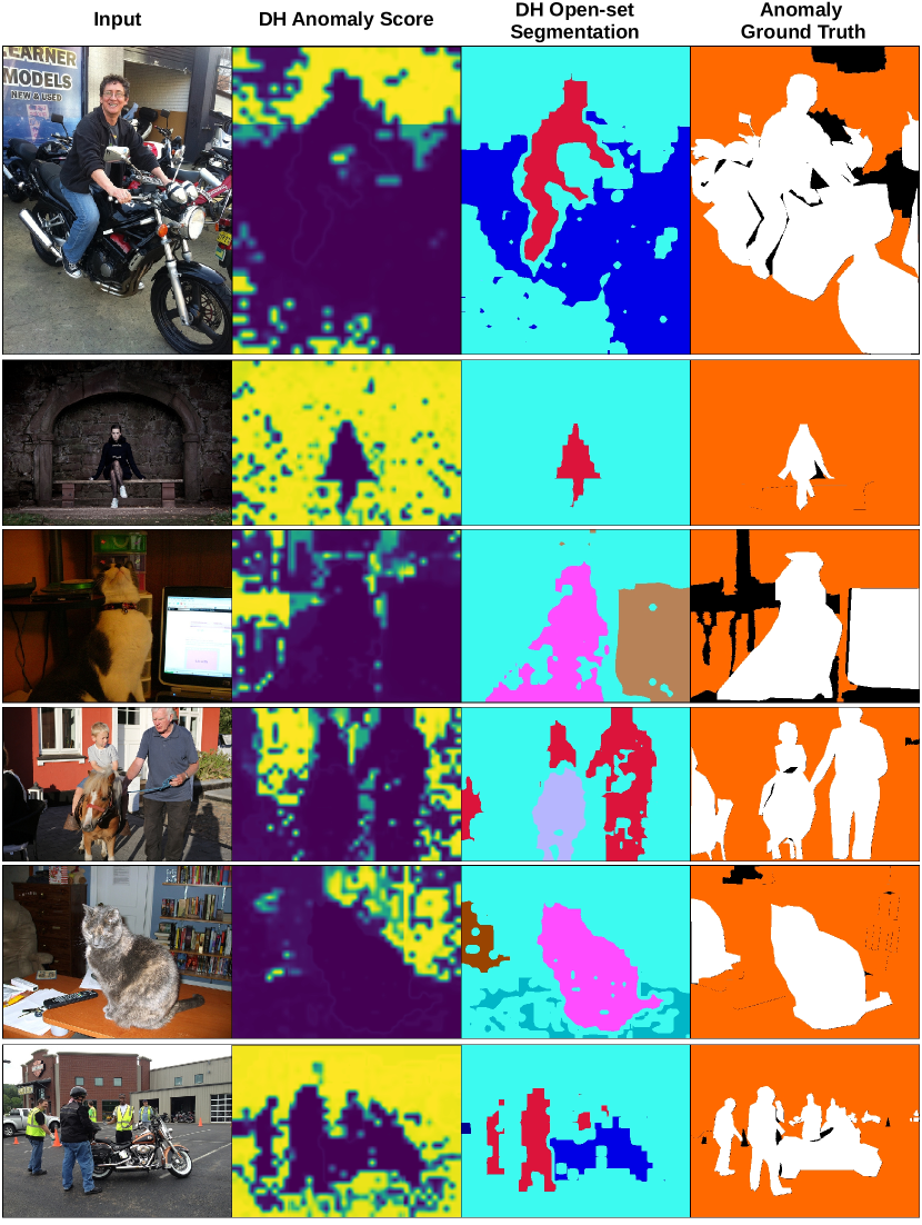
Figure 11: More qualitative examples of open-set segmentation on COCO. Unknown pixels are in cyan (third column) and correspond to ground truth denoted in orange (fourth column).

References

- [1] K. He, X. Zhang, S. Ren, and J. Sun, “Deep residual learning for image recognition,” in 2016 IEEE Conference on Computer Vision and Pattern Recognition, CVPR 2016, 2016, pp. 770–778.
- [2] Z. Liu, Y. Lin, Y. Cao, H. Hu, Y. Wei, Z. Zhang, S. Lin, and B. Guo, “Swin transformer: Hierarchical vision transformer using shifted windows,” in International Conference on Computer Vision, 2021.
- [3] M. Everingham, L. V. Gool, C. K. I. Williams, J. M. Winn, and A. Zisserman, “The pascal visual object classes (VOC) challenge,” Int. J. Comput. Vis., vol. 88, no. 2, pp. 303–338, 2010.
- [4] C. Farabet, C. Couprie, L. Najman, and Y. LeCun, “Learning hierarchical features for scene labeling,” IEEE Trans. Pattern Anal. Mach. Intell., vol. 35, no. 8, pp. 1915–1929, 2013.
- [5] S. Minaee, Y. Boykov, F. Porikli, A. Plaza, N. Kehtarnavaz, and D. Terzopoulos, “Image segmentation using deep learning: A survey,” IEEE Trans. Pattern Anal. Mach. Intell., vol. 44, no. 7, 2022.
- [6] E. Shelhamer, J. Long, and T. Darrell, “Fully convolutional networks for semantic segmentation,” IEEE Trans. Pattern Anal. Mach. Intell., vol. 39, no. 4, pp. 640–651, 2017.
- [7] L. Chen, G. Papandreou, I. Kokkinos, K. Murphy, and A. L. Yuille, “Deeplab: Semantic image segmentation with deep convolutional nets, atrous convolution, and fully connected crfs,” IEEE Trans. Pattern Anal. Mach. Intell., vol. 40, no. 4, pp. 834–848, 2018.
- [8] R. Strudel, R. G. Pinel, I. Laptev, and C. Schmid, “Segmenter: Transformer for semantic segmentation,” in 2021 IEEE/CVF International Conference on Computer Vision. IEEE, 2021, pp. 7242–7252.
- [9] X. Li, A. You, Z. Zhu, H. Zhao, M. Yang, K. Yang, S. Tan, and Y. Tong, “Semantic flow for fast and accurate scene parsing,” in European Conference on Computer Vision, 2020.
- [10] M. Orsic and S. Segvic, “Efficient semantic segmentation with pyramidal fusion,” Pattern Recognit., vol. 110, p. 107611, 2021.
- [11] H. Pan, Y. Hong, W. Sun, and Y. Jia, “Deep dual-resolution networks for real-time and accurate semantic segmentation of traffic scenes,” IEEE Trans. on Intelligent Transportation Systems, 2022.
- [12] H. Blum, P.-E. Sarlin, J. Nieto, R. Siegwart, and C. Cadena, “The fishyscapes benchmark: Measuring blind spots in semantic segmentation,” International Journal of Computer Vision, vol. 129, 2021.
- [13] C. González, K. Gotkowski, M. Fuchs, A. Bucher, A. Dadras, R. Fischbach, I. J. Kaltenborn, and A. Mukhopadhyay, “Distance-based detection of out-of-distribution silent failures for covid-19 lung lesion segmentation,” Medical Image Anal., vol. 82, 2022.
- [14] P. Pinggera, S. Ramos, S. Gehrig, U. Franke, C. Rother, and R. Mester, “Lost and found: detecting small road hazards for self-driving vehicles,” in International Conference on Intelligent Robots and Systems, IROS, 2016.
- [15] L. Ruff, J. R. Kauffmann, R. A. Vandermeulen, G. Montavon, W. Samek, M. Kloft, T. G. Dietterich, and K. Müller, “A unifying review of deep and shallow anomaly detection,” Proc. IEEE, vol. 109, no. 5, pp. 756–795, 2021.
- [16] T. E. Boult, S. Cruz, A. R. Dhamija, M. Günther, J. Henrydoss, and W. J. Scheirer, “Learning and the unknown: Surveying steps toward open world recognition,” in AAAI Conference on Artificial Intelligence. AAAI Press, 2019.
- [17] P. Bevandić, I. Krešo, M. Oršić, and S. Šegvić, “Dense open-set recognition based on training with noisy negative images,” Image and Vision Computing, vol. 124, p. 104490, 2022.
- [18] J. Cen, P. Yun, J. Cai, M. Y. Wang, and M. Liu, “Deep metric learning for open world semantic segmentation,” in International Conference on Computer Vision (ICCV), 2021.
- [19] S. Kong and D. Ramanan, “Opengan: Open-set recognition via open data generation,” IEEE Transactions on Pattern Analysis and Machine Intelligence, 2022.
- [20] H. Blum, P. Sarlin, J. I. Nieto, R. Siegwart, and C. Cadena, “Fishyscapes: A benchmark for safe semantic segmentation in autonomous driving,” in 2019 IEEE/CVF International Conference on Computer Vision Workshops. IEEE, 2019, pp. 2403–2412.
- [21] X. Du, Z. Wang, M. Cai, and Y. Li, “VOS: learning what you don’t know by virtual outlier synthesis,” in The Tenth International Conference on Learning Representations, ICLR 2022, 2022.
- [22] K. Lis, K. K. Nakka, P. Fua, and M. Salzmann, “Detecting the unexpected via image resynthesis,” in International Conference on Computer Vision, ICCV, 2019.
- [23] G. D. Biase, H. Blum, R. Siegwart, and C. Cadena, “Pixel-wise anomaly detection in complex driving scenes,” in Computer Vision and Pattern Recognition, CVPR, 2021.
- [24] T. Vojir, T. Šipka, R. Aljundi, N. Chumerin, D. O. Reino, and J. Matas, “Road anomaly detection by partial image reconstruction with segmentation coupling,” in International Conference on Computer Vision, ICCV, 2021.
- [25] T. DeVries and G. W. Taylor, “Learning confidence for out-of-distribution detection in neural networks,” CoRR, vol. abs/1802.04865, 2018.
- [26] A. Kendall and Y. Gal, “What uncertainties do we need in bayesian deep learning for computer vision?” in Neural Information Processing Systems, 2017.
- [27] E. T. Nalisnick, A. Matsukawa, Y. W. Teh, D. Görür, and B. Lakshminarayanan, “Do deep generative models know what they don’t know?” in International Conference on Learning Representations, 2019.
- [28] J. Serrà, D. Álvarez, V. Gómez, O. Slizovskaia, J. F. Núñez, and J. Luque, “Input complexity and out-of-distribution detection with likelihood-based generative models,” in 8th International Conference on Learning Representations, ICLR, 2020.
- [29] T. Lucas, K. Shmelkov, K. Alahari, C. Schmid, and J. Verbeek, “Adaptive density estimation for generative models,” in Neural Information Processing Systems, 2019.
- [30] L. H. Zhang, M. Goldstein, and R. Ranganath, “Understanding failures in out-of-distribution detection with deep generative models,” in International Conference on Machine Learning, ICML, 2021.
- [31] R. Chan, M. Rottmann, and H. Gottschalk, “Entropy maximization and meta classification for out-of-distribution detection in semantic segmentation,” in International Conference on Computer Vision, ICCV, 2021.
- [32] D. Hendrycks, M. Mazeika, and T. G. Dietterich, “Deep anomaly detection with outlier exposure,” in 7th International Conference on Learning Representations, ICLR, 2019.
- [33] K. Lee, H. Lee, K. Lee, and J. Shin, “Training confidence-calibrated classifiers for detecting out-of-distribution samples,” in 6th International Conference on Learning Representations, ICLR, 2018.
- [34] M. Grcic, P. Bevandic, and S. Segvic, “Densehybrid: Hybrid anomaly detection for dense open-set recognition,” in European Conference on Computer Vision, ECCV 2022. Springer, 2022.
- [35] M. Grcić, P. Bevandić, and S. Šegvić, “Dense open-set recognition with synthetic outliers generated by real NVP,” in 16th International Joint Conference on Computer Vision, Imaging and Computer Graphics Theory and Applications, VISIGRAPP, 2021.
- [36] D. M. Hawkins, Identification of Outliers, ser. Monographs on Applied Probability and Statistics. Springer, 1980.
- [37] D. Hendrycks and K. Gimpel, “A baseline for detecting misclassified and out-of-distribution examples in neural networks,” in 5th International Conference on Learning Representations, ICLR, 2017.
- [38] S. Liang, Y. Li, and R. Srikant, “Enhancing the reliability of out-of-distribution image detection in neural networks,” in 6th International Conference on Learning Representations, ICLR, 2018.
- [39] B. Lakshminarayanan, A. Pritzel, and C. Blundell, “Simple and scalable predictive uncertainty estimation using deep ensembles,” in Neural Information Processing Systems, 2017.
- [40] A. R. Dhamija, M. Günther, and T. E. Boult, “Reducing network agnostophobia,” in Annual Conference on Neural Information Processing Systems 2018, NeurIPS, 2018.
- [41] W. Liu, X. Wang, J. D. Owens, and Y. Li, “Energy-based out-of-distribution detection,” in NeurIPS, 2020.
- [42] V. Besnier, A. Bursuc, D. Picard, and A. Briot, “Triggering failures: Out-of-distribution detection by learning from local adversarial attacks in semantic segmentation,” in International Conference on Computer Vision, 2021.
- [43] L. Neal, M. L. Olson, X. Z. Fern, W. Wong, and F. Li, “Open set learning with counterfactual images,” in ECCV 2018 - 15th European Conference, Munich, German, 2018.
- [44] H. Zhang, A. Li, J. Guo, and Y. Guo, “Hybrid models for open set recognition,” in European Conference on Computer Vision, 2020.
- [45] P. Bevandic, I. Kreso, M. Orsic, and S. Segvic, “Simultaneous semantic segmentation and outlier detection in presence of domain shift,” in 41st DAGM German Conference, DAGM GCPR, 2019.
- [46] Y. Xia, Y. Zhang, F. Liu, W. Shen, and A. L. Yuille, “Synthesize then compare: Detecting failures and anomalies for semantic segmentation,” in European Conference on Computer Vision, ECCV, 2020.
- [47] V. Zavrtanik, M. Kristan, and D. Skocaj, “Reconstruction by inpainting for visual anomaly detection,” Pattern Recognit., 2021.
- [48] W. Grathwohl, K. Wang, J. Jacobsen, D. Duvenaud, M. Norouzi, and K. Swersky, “Your classifier is secretly an energy based model and you should treat it like one,” in 8th International Conference on Learning Representations, ICLR 2020, 2020.
- [49] Y. Tian, Y. Liu, G. Pang, F. Liu, Y. Chen, and G. Carneiro, “Pixel-wise energy-biased abstention learning for anomaly segmentation on complex urban driving scenes,” in European Conference on Computer, 2022.
- [50] C. Liang, W. Wang, J. Miao, and Y. Yang, “Gmmseg: Gaussian mixture based generative semantic segmentation models,” Advances in Neural Information Processing Systems, 2022.
- [51] W. J. Scheirer, A. de Rezende Rocha, A. Sapkota, and T. E. Boult, “Toward open set recognition,” IEEE Transactions on Pattern Analysis and Machine Intelligence, vol. 35, no. 7, pp. 1757–1772, 2013.
- [52] W. J. Scheirer, L. P. Jain, and T. E. Boult, “Probability models for open set recognition,” IEEE Trans. Pattern Anal. Mach. Intell., vol. 36, no. 11, pp. 2317–2324, 2014.
- [53] A. Bendale and T. E. Boult, “Towards open set deep networks,” in IEEE Conference on Computer Vision and Pattern Recognition, 2016.
- [54] S. Vaze, K. Han, A. Vedaldi, and A. Zisserman, “Open-set recognition: A good closed-set classifier is all you need,” in The Tenth International Conference on Learning Representations, ICLR 2022, 2022.
- [55] G. Chen, P. Peng, X. Wang, and Y. Tian, “Adversarial reciprocal points learning for open set recognition,” IEEE Trans. Pattern Anal. Mach. Intell., 2022.
- [56] C. Geng, S. Huang, and S. Chen, “Recent advances in open set recognition: A survey,” IEEE Trans. Pattern Anal. Mach. Intell., vol. 43, no. 10, pp. 3614–3631, 2021.
- [57] O. Zendel, K. Honauer, M. Murschitz, D. Steininger, and G. F. Dominguez, “Wilddash - creating hazard-aware benchmarks,” in European Conference on Computer Vision (ECCV), 2018.
- [58] R. Chan, K. Lis, S. Uhlemeyer, H. Blum, S. Honari, R. Siegwart, P. Fua, M. Salzmann, and M. Rottmann, “Segmentmeifyoucan: A benchmark for anomaly segmentation,” in Neural Information Processing Systems Track on Datasets and Benchmarks, 2021.
- [59] M. Sokolova and G. Lapalme, “A systematic analysis of performance measures for classification tasks,” Inf. Process. Manag., vol. 45, no. 4, pp. 427–437, 2009.
- [60] M. D. Scherreik and B. D. Rigling, “Open set recognition for automatic target classification with rejection,” IEEE Trans. Aerosp. Electron. Syst., vol. 52, no. 2, pp. 632–642, 2016.
- [61] C. Sakaridis, D. Dai, and L. V. Gool, “Map-guided curriculum domain adaptation and uncertainty-aware evaluation for semantic nighttime image segmentation,” IEEE Trans. Pattern Anal. Mach. Intell., vol. 44, no. 6, 2022.
- [62] U. Michieli and P. Zanuttigh, “Knowledge distillation for incremental learning in semantic segmentation,” Comput. Vis. Image Underst., vol. 205, p. 103167, 2021.
- [63] S. Uhlemeyer, M. Rottmann, and H. Gottschalk, “Towards unsupervised open world semantic segmentation,” in Uncertainty in Artificial Intelligence, 2022.
- [64] Y. Fu, X. Wang, H. Dong, Y. Jiang, M. Wang, X. Xue, and L. Sigal, “Vocabulary-informed zero-shot and open-set learning,” IEEE Trans. Pattern Anal. Mach. Intell., vol. 42, no. 12, 2020.
- [65] Y. Xian, C. H. Lampert, B. Schiele, and Z. Akata, “Zero-shot learning - A comprehensive evaluation of the good, the bad and the ugly,” IEEE Trans. Pattern Anal. Mach. Intell., vol. 41, no. 9, 2019.
- [66] T. Salimans, I. J. Goodfellow, W. Zaremba, V. Cheung, A. Radford, and X. Chen, “Improved techniques for training gans,” in Neural Information Processing Systems 2016, 2016, pp. 2226–2234.
- [67] Y. Du and I. Mordatch, “Implicit generation and modeling with energy based models,” in Neural Information Processing Systems 2019, NeurIPS 2019, 2019.
- [68] Y. Song and S. Ermon, “Generative modeling by estimating gradients of the data distribution,” in Neural Information Processing Systems 2019, NeurIPS 2019, 2019, pp. 11 895–11 907.
- [69] S. Kong and D. Ramanan, “An empirical exploration of open-set recognition via lightweight statistical pipelines,” 2021. [Online]. Available: https://openreview.net/forum?id=0Zxk3ynq7jE
- [70] Z. Zhao, L. Cao, and K. Lin, “Revealing distributional vulnerability of explicit discriminators by implicit generators,” CoRR, vol. abs/2108.09976, 2021.
- [71] M. Grcić, I. Grubišić, and S. Šegvić, “Densely connected normalizing flows,” in Neural Information Processing Systems, 2021.
- [72] M. Grcic, P. Bevandic, Z. Kalafatic, and S. Segvic, “Dense anomaly detection by robust learning on synthetic negative data,” CoRR, vol. abs/2112.12833, 2021.
- [73] M. Grcic, “Densehybrid source code: https://github.com/matejgrcic/DenseHybrid,” 2022.
- [74] D. Hendrycks, S. Basart, M. Mazeika, A. Zou, J. Kwon, M. Mostajabi, J. Steinhardt, and D. Song, “Scaling out-of-distribution detection for real-world settings,” in International Conference on Machine Learning, ICML, 2022.
- [75] B. Hariharan, P. Arbelaez, L. D. Bourdev, S. Maji, and J. Malik, “Semantic contours from inverse detectors,” in IEEE International Conference on Computer Vision, ICCV, 2011.
- [76] K. Lis, S. Honari, P. Fua, and M. Salzmann, “Detecting road obstacles by erasing them,” CoRR, vol. abs/2012.13633, 2020.
- [77] S. Jung, J. Lee, D. Gwak, S. Choi, and J. Choo, “Standardized max logits: A simple yet effective approach for identifying unexpected road obstacles in urban-scene segmentation,” in International Conference on Computer Vision, ICCV, 2021.
- [78] A. Malinin and M. J. F. Gales, “Predictive uncertainty estimation via prior networks,” in Neural Information Processing Systems, 2018.
- [79] K. Lee, K. Lee, H. Lee, and J. Shin, “A simple unified framework for detecting out-of-distribution samples and adversarial attacks,” in Neural Information Processing Systems, NeurIPS, 2018.
- [80] J. Steinhardt and P. Liang, “Unsupervised risk estimation using only conditional independence structure,” in Neural Information Processing Systems 2016, 2016, pp. 3657–3665.
- [81] P. Oza and V. M. Patel, “C2ae: Class conditioned auto-encoder for open-set recognition,” in Proceedings of the IEEE/CVF Conference on Computer Vision and Pattern Recognition (CVPR), June 2019.
- [82] G. Franchi, A. Bursuc, E. Aldea, S. Dubuisson, and I. Bloch, “TRADI: tracking deep neural network weight distributions,” in 16th European Conference on Computer Vision, ECCV, 2020.
- [83] Y. Sun, C. Guo, and Y. Li, “React: Out-of-distribution detection with rectified activations,” in NeurIPS, 2021.
- [84] T. Zhou, W. Wang, E. Konukoglu, and L. V. Gool, “Rethinking semantic segmentation: A prototype view,” in IEEE/CVF Conference on Computer Vision and Pattern Recognition, CVPR, 2022.
- [85] B. Cheng, A. G. Schwing, and A. Kirillov, “Per-pixel classification is not all you need for semantic segmentation,” in Neural Information Processing Systems, 2021.
- [86] I. Kreso, J. Krapac, and S. Segvic, “Efficient ladder-style densenets for semantic segmentation of large images,” IEEE Trans. Intell. Transp. Syst., vol. 22, 2021.
- [87] M. Cordts, M. Omran, S. Ramos, T. Rehfeld, M. Enzweiler, R. Benenson, U. Franke, S. Roth, and B. Schiele, “The cityscapes dataset for semantic urban scene understanding,” in IEEE Conference on Computer Vision and Pattern Recognition, CVPR, 2016.
- [88] G. Neuhold, T. Ollmann, S. R. Bulò, and P. Kontschieder, “The mapillary vistas dataset for semantic understanding of street scenes,” in IEEE International Conference on Computer Vision, 2017.
- [89] Y. Zhu, K. Sapra, F. A. Reda, K. J. Shih, S. D. Newsam, A. Tao, and B. Catanzaro, “Improving semantic segmentation via video propagation and label relaxation,” in IEEE Conference on Computer Vision and Pattern Recognition, CVPR, 2019.