Out of equilibrium dynamics of repulsive ranked diffusions: the expanding crystal

Abstract

We study the non-equilibrium Langevin dynamics of $N$ particles in one dimension with Coulomb repulsive linear interactions. This is a dynamical version of the so-called jellium model (without confinement) also known as ranked diffusion. Using a mapping to the Lieb-Liniger model of quantum bosons, we obtain an exact formula for the joint distribution of the positions of the $N$ particles at time $t$, all starting from the origin. A saddle point analysis shows that the system converges at large time to a linearly expanding crystal. Properly rescaled, this dynamical state resembles the equilibrium crystal in a time dependent effective quadratic potential. This analogy allows to study the fluctuations around the perfect crystal, which, to leading order, are Gaussian. There are however deviations from this Gaussian behavior, which embody long-range correlations of purely dynamical origin, characterized by the higher order cumulants of, e.g., the gaps between the particles, that we calculate exactly. We complement these results using a recent approach by one of us in terms of a noisy Burgers equation. In the large $N$ limit, the mean density of the gas can be obtained at any time from the solution of a deterministic viscous Burgers equation. This approach provides a quantitative description of the dense regime at shorter times. Our predictions are in good agreement with numerical simulations for finite and large $N$.

I Introduction and the main results

The Coulomb potential in one dimension is linear in the distance. Particles interacting with this potential have been much studied. Many of these studies address the canonical equilibrium at some temperature $T$. In the attractive case it is related to the statistical mechanics of the self-gravitating $1d$ gas Rybicki ; Sire ; Kumar2017 . In the repulsive case, and in presence of a background charge or in a finite box, it is called jellium and its fluctuations at equilibrium have been well studied Lenard ; Prager ; Baxter ; Dean1 ; Tellez ; Lewin , with a recent renewed interest, in particular in edge fluctuations and large deviations SatyaJellium1 ; SatyaJellium2 ; SatyaJellium3 ; Chafai_edge ; Flack22 .

In this paper, we study the out of equilibrium dynamics of this system and demonstrate that it exhibits rather rich and interesting behaviors, as a function of time. In $1d$, the Coulomb force (either attractive or repulsive) acting on each particle is proportional to its rank, i.e., the number of particles in its front minus the number of particles at the back of it. The Langevin dynamics of this system is called ranked diffusion. The diffusion of $N$ particles in $1d$ under a drift which depends only on their ranks has been studied in finance Banner and in mathematics Pitman ; OConnell .

Recently the non-equilibrium dynamics of this model was studied PLDRankedDiffusion using a mapping to the Lieb-Liniger model, or $1d$ delta Bose gas. Since the latter is integrable by Bethe ansatz, it allows in principle to obtain formula for non-equilibrium observables in the ranked diffusion model for any $N$. In practice however this approach is analytically complicated, and not all initial conditions can be easily treated. Hence this program has yet to be fully completed. Furthermore the exact solution does not allow to add an external potential, since it breaks integrability. Another more versatile approach was thus also studied in PLDRankedDiffusion , which exploits a connection to the noisy Burgers equation. This method is most efficient to study the large $N$ limit, where the effect of the noise term is reduced.

In this paper we focus on the repulsive gas and show that many exact results on its dynamics can be derived using the aforementioned two complementary approaches. We study a gas of $N$ particles on the line, in the absence of external potential, performing thermal diffusion at temperature $T$, and mutually interacting via the linear Coulomb potential of strength $c>0$ (see the definition of the model in (4)). In addition to diffusion, each particle thus experiences a drift proportional to its rank, typically of order $O(c\,N)$ for large $N$. There is no additional hard-core interaction and therefore the particles are free to cross each other. We focus on the case where all the particles start at $t=0$ from the origin at $x=0$. Several realizations of this dynamics are shown in Fig. 1 for $N=500$, where one can see that there are several interesting regimes as a function of time. Since the gas is expanding from a point source, it is dense at short times and particles experience many mutual crossings (see figure a) in Fig. 1). At large time, the gas is diluted and the particles are far from each other, but, as we will show, they nevertheless form a well ordered expanding crystal due to the long range nature of the interaction (see figure c) in Fig. 1). In fact we find that when $N$ is large one can distinguish three different regimes (see figures a),b),c) in Fig. 1). Indeed, there are two characteristic length scales associated respectively to the diffusion and the drift, namely

$$\ell_{T}\sim\sqrt{2Tt}\quad,\quad\ell\sim 2cNt\;.$$ (1)

The first length $\ell_{T}$ is the typical thermal diffusion length of independent particles. Since the rightmost (respectively leftmost) particle experiences a drift $\sim cN$ (respectively $-cN)$ the second length $\ell$ is the total size of the gas at large time. Comparing the two length scales we see that there is a characteristic time scale

$$t_{1}^{*}\sim\frac{1}{N^{2}}\frac{T}{c^{2}}$$ (2)

such that for $t<t_{1}^{*}$ the diffusion dominates over the drift. In that regime, which we call regime I, the particles are almost independent and the gas is very dense (see figure a) in Fig. 1). For time $t>t_{1}^{*}$ the drift, i.e., the interaction, dominates over the diffusion. This is regime II, where the gas evolves from being dense to being dilute. The crossover from regime I to regime II in the behavior of the size of the gas (i.e. distance between rightmost and leftmost particle) is shown in the right upper panel of Fig. 1. As we will show, in regime II as time increases, the density converges to a square shape, being uniform on $[-\ell/2,\ell/2]$, with a boundary layer at the two edges of size $\ell_{T}\sim\sqrt{2Tt}\ll\ell$. In this regime II however the particles still experience many crossings, (see panel b in Fig. 1) and the size of the boundary layer is still much larger than the interparticle distance $a=\ell/N=2ct$. As time further increases the density becomes so low that the particles cross each other only rarely. This happens when $a\sim\ell_{T}$ which defines the second time scale

$$t_{2}^{*}\sim\frac{T}{c^{2}}$$ (3)

Beyond this time scale, for $t\gg t_{2}^{*}$, one has $\ell_{T}\ll a=2ct$, and the particles are well separated and do not cross anymore: this is regime III (dilute regime). These three regimes, together with the formation of a square density, can be clearly seen in Fig. 1. Note that if the initial condition has instead a finite extension $\ell_{0}$, there exists another time scale $t^{*}_{0}\sim\ell_{0}/(cN)$ at which most features of the initial density are erased and the plateau forms. Here we mainly focus on the case $\ell_{0}=0$ so this time scale is absent. Note that for finite $N$ these time scales are all identical and there is only a short time regime $c^{2}t/T\ll 1$ and a large time regime $c^{2}t/T\gg 1$.

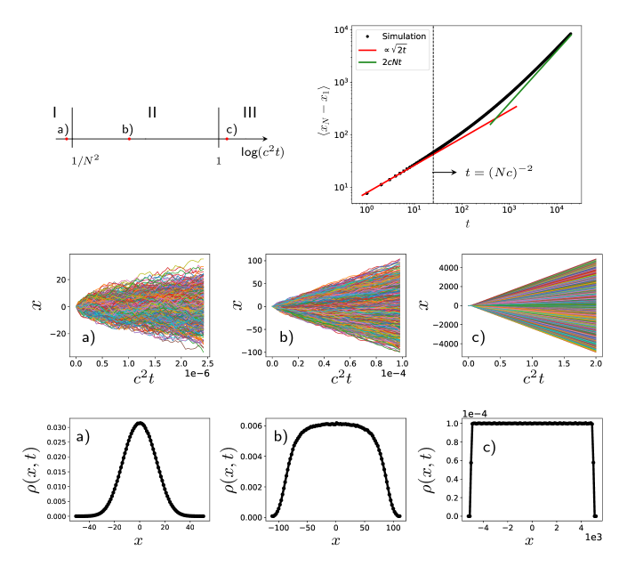
Figure 1: Upper panel left: summary of the values of the dimensionless final time $c^{2}t$ used in the figures a), b) and c) below. Upper panel right: size of the gas as a function of time (in a log-log scale) which shows a crossover between the regimes I and II and time $t_{1}^{*}=T/(Nc)^{2}$ which is indicated by a vertical dashed line. Symbols are the results of numerical simulations. The red solid line at short time represents the prediction in regime I, $\ell_{T}=\sqrt{2\,T\,t}$ (here $T=1$), and the green one at larger time corresponds to the prediction in regime II, $\ell=2Nct$ [see Eq. (1)]. Middle panel, figures a-c: examples of trajectories $x_{i}(t)$ vs $t$ of $N=500$ particles evolving via the Langevin equation in Eq. (4). One can identify three different regimes determined by the value of the dimensionless time $c^{2}t$. Bottom panel, figures a-c: corresponding densities of particles $\rho(x,t_{f})$ at the final time $t=t_{f}$ for each of the three top figures. They are obtained by averaging over $10^{4}$ realizations of the noise, and using $100$ bins to construct the histograms. Here for convenience we chose $t_{f}=50$ and varied $c$. These three values fall in each of the three regimes I-III discussed in the text.

These three regimes exhibit quite different density and particle correlation properties. To obtain a quantitative description of the system, we first derive in Section II, using the Bethe ansatz, an integral formula for the joint probability distribution function (PDF) of the positions of the particles, all starting from the origin, given in Eq. (12), which is exact for any $N$ and $t$. By analyzing this formula via a saddle point method, we obtain in Section III the asymptotic form of the joint PDF at large time, see Eq. (25). It is a priori valid for any fixed $N$ and for $c^{2}t/T\gg 1$. At large $N$ it thus describes the regime III (the dilute regime). From that formula we find that in that regime the system is a well ordered expanding crystal, with most probable particle positions $x_{j}=c(N+1-2j){t}$. To compute the fluctuations of the particle positions in this crystal, we proceed in two stages. We first approximate the formula (25) for the joint PDF by neglecting the rational prefactor, in which case it becomes formally identical to the equilibrium distribution given in Eq. (32) of the $1d$ jellium model [defined in (28)]. Although this analogy holds for any $N$, it is especially useful for large $N$, where many results are known for the jellium model SatyaJellium1 ; SatyaJellium2 . We find that, within that approximation, the regime III corresponds to the jellium model with a dimensionless interaction strength $\alpha\gg 1$. It correctly predicts the leading order of the fluctuations of the particle positions around their ordered positions, which in this regime are small and independent Gaussian random variables. The amplitude of these fluctuations are of the order of the diffusion length $\ell_{T}\sim\sqrt{2Tt}$. Next, we treat more accurately the asymptotic joint PDF in Eq. (25), and show that there are non-trivial additional position fluctuations, which are of order $O(T/c)$. We characterize them completely by computing analytically all the joint cumulants of the particle positions, given in Eq. (68). These formulae show that there are non-trivial correlations of purely dynamical origin, which persist for $c^{2}t/T\gg 1$ and go beyond the analogy with the equilibrium jellium model. It is yet unclear how to extend these results to the case $c^{2}t/T=O(1)$ and in particular to the more correlated regime II, i.e., for $c^{2}t/T\ll 1$, where the particle crossings cannot be ignored. We expect that some of these effects will be captured by the analogy with the jellium model at finite interaction strength $\alpha$, but that additional dynamical correlations will also exist. Note that we also treat exactly the case $N=2$ which is quite instructive, in particular to analyze systematically the role of the initial condition (which we were not able to do for general $N$).

Next, in Section IV, we recall the hydrodynamic approach of PLDRankedDiffusion using the Burgers equation, which gives a prediction for the time dependent density at large $N$ for arbitrary time. It thus allows to derive analytical formula for the time evolution of the average particle density within the crossover between the regimes I and II, when the gas is still sufficiently dense. For that study it is convenient to scale $c=\gamma/N$ with $\gamma=O(1)$ in which case the time scale $t_{1}=O(1)$. Finally, we perform numerical simulations and compare the results with the predictions of both methods (the Bethe ansatz and the hydrodynamic approach). We confirm the Gaussian character of the fluctuations in regime III and we test the accuracy of the predictions for the density using the deterministic Burgers equation.

Finally, in Appendix A we study in detail the case $N=2$. In Appendix B we study the corrections to the cumulants of the particle positions, which are exponentially small at large time. In Appendix C we derive the form of the boundary layer for the Burgers equation.

II Model and main formula

In this paper we consider $N$ particles on the real line at positions $x_{i}(t)$, $i=1,\dots,N$, evolving according to the Langevin equation

$$\frac{dx_{i}}{dt}=-\partial_{x_{i}}W(\vec{x})+\sqrt{2T}\xi_{i}(t)=-c\sum_{j=1}^{N}{\rm sgn}(x_{j}-x_{i})+\sqrt{2T}\xi_{i}(t)\;,$$ (4)

where $\xi_{i}(t)$ are $N$ unit independent white noises with zero mean $\langle\zeta_{i}(t)\rangle=0$ and delta-correlator $\langle\zeta_{i}(t)\zeta_{j}(t^{\prime})\rangle=\delta_{i,j}\delta(t-t^{\prime})$. Here $T$ is the temperature, and by convention ${\rm sgn}(0)=0$. The particles interact via the linear pairwise potential energy $W(\vec{x})=-c\sum_{i<j}|x_{i}-x_{j}|$ where we denote ${\vec{x}}=\{x_{i}(t)\}_{i=1,\dots,N}$. The particles may cross (and they will) and if we denote $x_{(i)}(t)$ the ordered sequence of their positions at time $t$ in increasing order, then the ordered particle $x_{(i)}$ feels a drift

$$\delta_{i}=-c\sum_{j=1}^{N}{\rm sgn}(x_{(j)}-x_{(i)})=-c\,(N+1-2i)\;,$$ (5)

which depends on the label/rank $i$ of the particle: this is just proportional to the number of particles in front minus the number of particles at the back of the $i$-th particle. For $c>0$ the interaction is thus repulsive, the case considered here.

Next one introduces the probability density function (PDF), $P(\vec{x},t)$, of a given configuration ${\vec{x}}$ of the particles. It satisfies the Fokker-Planck (FP) equation

$$\partial_{t}P=-{\cal H}_{\rm FP}P=\sum_{i}[T\partial_{x_{i}}^{2}-c\partial_{x_{i}}\sum_{j}{\rm sgn}(x_{i}-x_{j})]P\;.$$ (6)

For $c<0$ this equation formally admits a zero current stationary solution

$$P_{0}(\vec{x})=\frac{1}{Z_{N}}\Psi_{0}(\vec{x})^{2}\quad,\quad\Psi_{0}(\vec{x}):=e^{-\frac{1}{2T}W(\vec{x})}=e^{\frac{c}{4T}\sum_{i,j=1}^{N}|x_{i}-x_{j}|}\;,$$ (7)

where $Z_{N}$ is a normalization constant. For $c>0$ this solution is however not normalizable, and is not the stationary state. Indeed, in the absence of external potential the gas expands linearly with time PLDRankedDiffusion , an expansion that we will study here in more details.

It is useful to note at this stage that the two parameters of the model, $T$ and $c$, can be absorbed in a change of units. More precisely $T/c$ is a length scale and $T/c^{2}$ is a time scale. In terms of these scales one can always write

$$P(\vec{x},t)={\left(\frac{c}{T}\right)^{N}}\tilde{P}\left(\frac{c\,\vec{x}}{T},\frac{c^{2}t}{T}\right)\;,$$ (8)

where $\tilde{P}(\vec{x},t)$ is the PDF for the model with $c=T=1$. We have seen in the introduction that at large $N$ there are several distinct time scales. These can be explored conveniently by scaling $c$ in various ways with $N$. Hence we will not fix the parameter $c$. However for the calculations in the remainder of this section, as well as in Section III, we will set $T=1$. Since $c$ and $T$ can be absorbed in the units, there is no intrinsic dimensionless parameter in the model, besides $N$ and some parameter characterizing the initial condition, e.g such as $c{\ell}_{0}/T$, if ${\ell}_{0}$ is the initial interparticle distance (below we focus on $\ell_{0}=0$). Hence all the regimes can be obtained by looking at the particular scale of interest.

Let us consider now the delta initial condition where all particles are at the same position $\vec{x}(0)=\vec{0}$ in space at time $t=0$

$$P(\vec{x},t=0)=\prod_{i}\delta(x_{i})\;.$$ (9)

Hence $P(\vec{x},t)$ is the Green’s function of the Fokker-Planck operator ${\cal H}_{\rm FP}$, i.e., $P(\vec{x},t)=G_{\rm FP}(\vec{x},\vec{0},t)$ where $G_{\rm FP}(\vec{x},\vec{y},t)=\langle\vec{x}|e^{-t{\cal H}_{\rm FP}}|\vec{y}\rangle$. It is easy to check that

$$G_{\rm FP}(\vec{x},\vec{y},t)=\frac{\Psi_{0}(\vec{x})}{\Psi_{0}(\vec{y})}G_{s}(\vec{x},\vec{y},t)e^{E_{0}\,t}\quad{\rm with}\quad E_{0}=-\frac{c^{2}}{12}(N^{3}-N)\;,$$ (10)

where $G_{s}(\vec{x},\vec{y},t)$ is the Green’s function of the Schrödinger Hamiltonian ${\cal H}_{s}$, i.e., the solution for $t>0$ of $\partial_{t}G_{s}=-{\cal H}_{s}G$ with initial condition $G_{s}(\vec{x},\vec{y},t=0)=\prod_{i}\delta(x_{i})$. Here ${\cal H}_{s}$ is the Lieb-Liniger Hamiltonian LL

$${\cal H}_{s}=-\sum_{i}\partial_{x_{i}}^{2}+2c\sum_{1\leq i<j\leq N}\delta(x_{i}-x_{j})$$ (11)

which describes quantum particles with delta repulsive interactions. Note that the initial condition (9) is symmetric in the exchange of particles. In this symmetric sector the model (11) is also called the delta Bose gas, which is integrable by the Bethe ansatz LL ; GaudinBook . The quantity $E_{0}$ is the ground state energy of the model. The relation (10) can be checked by applying ${\cal H}_{\rm FP}$ on each side.

For the delta initial condition the Schrodinger problem can be solved and there exists a multiple integral formula for $G_{s}(\vec{x},\vec{0},t)$ valid for all times. From Proposition 6.2.3 (Eq. (6.6)) in BorodinCorwinMacDo (for earlier works see TWBoseGas ; GaudinBook ), and using (10) we obtain for $c>0$, for any $N$ and $t>0$ and for the sector $x_{1}\leq x_{2}\leq\dots\leq x_{N}$

$${P(\vec{x},t)=G_{\rm FP}(\vec{x},\vec{y}=\vec{0},t)=}e^{\frac{c}{4}\sum_{i,j=1}^{N}|x_{i}-x_{j}|}e^{E_{0}t}\int_{\mathbb{R}}\frac{dk_{1}}{2\pi}\dots\int_{\mathbb{R}}\frac{dk_{N}}{2\pi}\prod_{1\leq a<b\leq N}\frac{ik_{a}-ik_{b}}{ik_{a}-ik_{b}+c}\quad e^{-t\sum_{j=1}^{N}k_{j}^{2}+i\sum_{j=1}^{N}x_{j}k_{j}}\;,$$ (12)

where the variables $k_{i}$ are integrated over the real axis and $E_{0}$ is given in Eq. (10). Being a fully symmetric function of its arguments, $P(\vec{x},t)$ is obtained in the other sectors by symmetry. Note that, by construction, $P(\vec{x},t)$ in Eq. (12) is normalized to unity on $\mathbb{R}^{N}$ for all time $t\geq 0$, although this property is not so obvious to check from (12). This explicit expression in Eq. (12) is our main formula, which we analyze in the following sections.

III Time evolution of $P(\vec{x},t)$

In this section, we analyze the time-evolution of $P(\vec{x},t)$. In the first subsection III.1, we verify the validity of the formula (12) for $N=2$ by finding directly the exact solution of the Fokker-Planck equation (6). The case $N=2$ being already very instructive, we study in details its large time asymptotics. In the next subsection III.2, we perform a saddle-point analysis of the formula in (12) for large $t$, for any fixed $N$. In subsection III.3, we make an analogy between this expanding Coulomb gas at large $t$ and the static properties of a one-dimensional one-component plasma in a harmonic potential. Finally, in subsection III.4 we obtain the higher cumulants of the position fluctuations from a more precise analysis of the large time limit.

III.1 Two particles $N=2$

Let us start with two particles, i.e., $N=2$. Introducing the center of mass coordinate $x(t)=\frac{1}{2}(x_{1}(t)+x_{2}(t))$ and the relative coordinate $y(t)=x_{2}(t)-x_{1}(t)$, the Fokker Planck equation (6) is easily solved directly by a Laplace transform. Denoting $P(y,t)$ the PDF of $y(t)$ (with a slight abuse of notation) we find (see details in Appendix A)

$$\tilde{P}(y,s)=\int_{0}^{+\infty}dte^{-st}P(y,t)=\frac{e^{\frac{c}{2}|y|}}{2(c+\sqrt{c^{2}+2s})}e^{-\frac{1}{2}\sqrt{c^{2}+2s}|y|}\;,$$ (13)

which upon Laplace inversion gives

$$P(y,t)=\frac{e^{-\frac{(|y|-2ct)^{2}}{8t}}}{2\sqrt{2\pi}\sqrt{t}}-\frac{1}{4}ce^{c|y|}\text{erfc}\left(\frac{2ct+|y|}{2\sqrt{2}\sqrt{t}}\right)\;,$$ (14)

which is normalized to unity, i.e., $\int_{-\infty}^{+\infty}dyP(y,t)=1$ and satisfies the initial condition $P(y,0)=\delta(y)$. Here ${\rm erfc(z)}=2/\sqrt{\pi}\int_{z}^{\infty}e^{-u^{2}}\,du$. We now want to check that the general formula in Eq. (12) for the joint distribution of $N$ particles also leads to the result in Eq. (14) for $N=2$. Indeed, in Appendix A, we show this explicitly. The time evolution of $P(y,t)$ from (14) is plotted in Fig. 2.

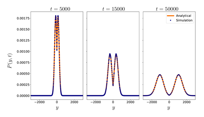
Figure 2: The probability distribution $P(y,t)$ of the relative coordinate $y(t)=x_{2}(t)-x_{1}(t)$ for two particles for different times ($t=5000$, $t=15000$, $t=50000$). The blue dots are obtained by the simulation with $c=0.01$, $T=1$ and averaging over $10^{6}$ realizations. The solid orange lines represent the analytical expression for the distribution derived in Eq. (14). One can see that the distribution becomes bimodal at large time.

At large time it becomes a bimodal distribution centered around $y\simeq\pm 2ct$. For fixed $y=O(1)$ one finds, as $t\to\infty$

$$P(y,t)\simeq\frac{(c|y|+2)e^{-\frac{(|y|-2ct)^{2}}{8t}}}{4\sqrt{2\pi}c^{2}t^{3/2}}{\simeq\frac{(c|y|+2)e^{\frac{|y|}{2}}}{4\sqrt{2\pi}c^{2}t^{3/2}}e^{-\frac{c^{2}t}{2}}}\;.$$ (15)

where in the last equation we used that $|y|=O(1)$. On the other hand, if one scales $y=zt$ with fixed $z=O(1)$ one finds

$$P(y,t)\simeq\frac{|z|e^{-\frac{1}{8}t(|z|-2c)^{2}}}{2\sqrt{2\pi t}(|z|+2c)}\;.$$ (16)

On these scales it thus converges, as $t\to\infty$, to a pair of delta-functions at $z=\pm 2$, each of weight $1/2$. For $t$ large but finite one can check that the total probability weight in the asymptotic form (16) is slightly less than unity, but converges to unity as $t\to+\infty$. Note that although the exponential factor is the same in (15) and in (16), the prefactors in each formula are distinct: only the large $|y|=O(1)$ limit of (15) matches the small $|z|=O(1)$ limit of (16).

One can also calculate the cumulants of the random variable $|y|-2ct$. While more detailed expressions are given in Appendix A.3, here we simply indicate their leading behaviors at large time. We obtain

$$\langle|y|\rangle-2ct\simeq 1/c+O(t^{-3/2}e^{-c^{2}t/2})\;,$$ (17)

$$\langle(|y|-2ct)^{2}\rangle_{c}\simeq 4t-3/c^{2}+O(t^{-1/2}e^{-c^{2}t/2})\;,$$ (18)

$$\langle(|y|-2ct)^{3}\rangle_{c}\simeq 14/c^{3}+O(t^{1/2}e^{-c^{2}t/2})\;,$$ (19)

$$\langle(|y|-2ct)^{4}\rangle_{c}\simeq-90/c^{4}+O(t^{3/2}e^{-c^{2}t/2})\;.$$ (20)

where $\langle\dots\rangle_{c}$, with a subscript $c$, denotes cumulants (not to be confused with the interaction parameter $c$). Interestingly, while the variance of $|y|$ grows linearly with $t$ for large $t$, the higher cumulants converge to a constant. The leading fluctuations are thus Gaussian and diffusive $O(\sqrt{t})$, but there are some additional $O(1)$ non Gaussian fluctuations, as encoded in the higher order cumulants. As we will see below these features will extend to any $N$, hence $N=2$ is a useful testing ground for general $N$. One can check (e.g. numerically) that the leading orders (i.e., up to $O(1)$) of the cumulants (17)-(20) are reproduced if one uses the asymptotic form (16), which thus captures the $O(1)$ non Gaussian fluctuations at large time. In addition, in Section III.4 we obtain an exact formula for the $O(1)$ leading orders of all the cumulants at large time, i.e, for any $N$ (hence including $N=2$), based on a saddle point method. To obtain them we show that for $c^{2}t\gg 1$ one can restrict to an ordered sector $x_{1}<\dots<x_{N}$ and neglect the events when particles cross. These events are only responsible for the exponential corrections to the cumulants (e.g. $e^{-c^{2}t/2}$ for $N=2$ in (17)-(20)). Finally, we have checked the predictions of (17)-(20) by a numerical solution of the Langevin equation, the results are presented in Fig. 3.

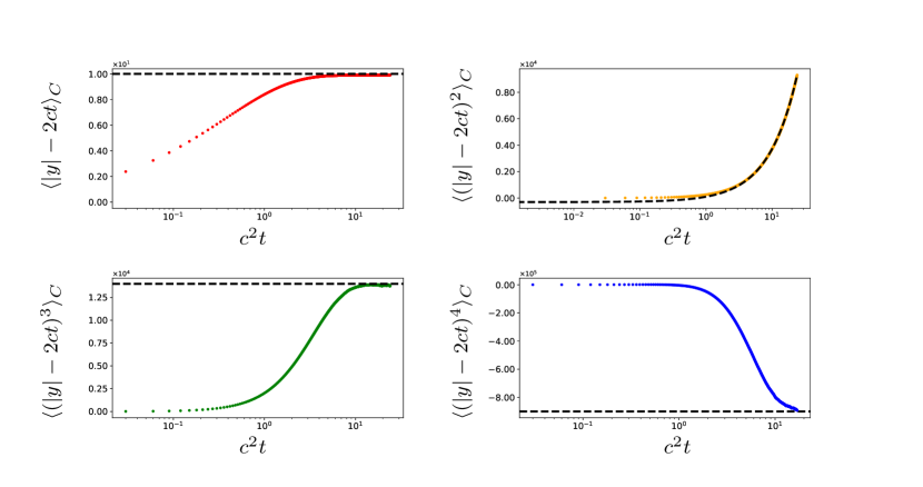
Figure 3: Plot of first four cumulants $\langle(|y|-2ct)^{k}\rangle_{c}$, with $k=1,2,3,4$ as a function of dimensionless time $c^{2}t$ (in logarithmic scale) from the numerical solution of the Langevin equation, as compared to the analytical prediction at large time from Eqs. (17)-(20) (black dashed line). We chose $c=0.1$ and averaged over $2\times 10^{8}$ realizations of the noise.

III.2 Saddle-point analysis at late times $t$ for fixed $N$

Let us now consider the general case of $N$ particles. We start from the general formula (12) for the joint PDF restricted to the sector $x_{1}\leq x_{2}\leq\dots\leq x_{N}$. Let us define the rescaled variables $x_{j}=z_{j}t$. In terms of these variables the joint PDF $P(\vec{x},t)$ reads, using $E_{0}$ from Eq. (10) and with $z_{1}\leq z_{2}\leq\dots\leq z_{N}$,

$$P(\vec{x},t)=\int_{\mathbb{R}}\frac{dk_{1}}{2\pi}\dots\int_{\mathbb{R}}\frac{dk_{N}}{2\pi}e^{t\,[\frac{c}{4}\sum_{i,j=1}^{N}|z_{i}-z_{j}|-\sum_{j=1}^{N}k_{j}^{2}+i\sum_{j=1}^{N}z_{j}k_{j}-\frac{c^{2}}{12}N(N^{2}-1)]}\prod_{1\leq a<b\leq N}\frac{ik_{a}-ik_{b}}{ik_{a}-ik_{b}+c}\;.$$ (21)

Let us consider now the regime of large time, $t\to+\infty$ with fixed $N$, and with the $z_{j}=O(1)$, i.e., $x_{j}=O(t)$. For large $t$, the expression multiplying $t$ in the exponent of the integrand in Eq. (21) gets minimized at the saddle point with the values

$$k_{j}^{*}=\frac{iz_{j}}{2}\;,$$ (22)

which are on the imaginary $k$-axis. Note that the original integrals in (21) are on the real $k$-axis. Hence we need to deform the contour in the complex $k$-plane so that it passes through the saddle point and picks up the leading contribution for large $t$. This can be done without crossing the poles in the prefactor in (21), by deforming the contours for each $k_{j}$ successively maintaining the condition ${\rm Im}\,k_{N}>\cdots>{\rm Im}\,k_{1}$. This gives

$$P(\vec{x},t)\simeq\frac{1}{(4\pi t)^{N/2}}e^{\frac{tc}{4}\sum_{i,j=1}^{N}|z_{i}-z_{j}|-t\sum_{j}\frac{z_{j}^{2}}{4}}e^{-\frac{c^{2}}{12}N(N^{2}-1)t}\prod_{1\leq a<b\leq N}\frac{z_{b}-z_{a}}{z_{b}-z_{a}+2c}\;.$$ (23)

Note that since $z_{b}>z_{a}$ for $b>a$ there are no poles in the double product. For $N=2$ one can check that one recovers the expression in (16), which is a bimodal distribution at large time. As was discussed there, it is valid for $c^{2}t\gg 1$, and so is (23) for any finite $N$.

One can rewrite this formula to make more explicit the most probable position of each particle. Using the equality, for $z_{1}\leq z_{2}\dots\leq z_{N}$

$$\frac{c}{4}\sum_{i,j=1}^{N}|z_{i}-z_{j}|=-\frac{c}{2}\sum_{j=1}^{N}(N+1-2j)z_{j}$$ (24)

and completing the square, one finds

$$P(\vec{x},t)\simeq\frac{1}{(4\pi t)^{N/2}}e^{-\frac{t}{4}\sum_{j=1}^{N}(z_{j}-c(2j-N-1))^{2}}\prod_{1\leq a<b\leq N}\frac{z_{b}-z_{a}}{z_{b}-z_{a}+2c}\quad,\quad\text{for}\,\,z_{1}\leq z_{2}\dots\leq z_{N}\;.$$ (25)

The most probable values for the rescaled positions at large time are thus

$$\frac{x_{j}}{t}=z_{j}=c(2j-N-1)\;.$$ (26)

These positions form a perfect crystal with uniform spacing $2c$ which extends from $z_{1}=-c(N-1)$ to $z_{N}=c(N-1)$. One can check that for $t\to+\infty$ the normalization of the formula (25) inside the ordered sector is $1/N!$, as expected. Indeed in that limit (i) the fluctuations of the $z_{j}$’s around the most probable values are vanishing as $1/\sqrt{t}$ (ii) in the prefactor one can simply replace the $z_{a}$ by their most probable values, $z_{a}=c(2j-N-1)$ and one finds that the double product over $a$ and $b$ in (25) simply equals $1/N!$.

We will now, and in the following subsections, ask about the deviations around the perfect crystal. Let us denote them as

$$\delta x_{j}=x_{j}-c\,t(2j-N-1)$$ (27)

The quadratic form in the exponential in (25) can be rewritten simply as $-\sum_{j}\frac{\delta x_{j}^{2}}{4t}$. This would suggest that the fluctuations of are the $\delta x_{j}$’s are independent and Gaussian for each particle with a width given by the diffusion length, $\ell_{T}=\sqrt{2t}$, independently of $N$. This is not the case however for the two following reasons:

• there is an ordering condition between the particles,

• there is the double product prefactor in (25).

Nevertheless, it is true that if one scales $\delta x_{j}=\sqrt{2t}\,\delta\tilde{x}_{j}$ with $\delta\tilde{x}_{j}=O(1)$ the joint PDF of the $\delta\tilde{x}_{j}$’s converges, as $c^{2}t\to+\infty$, to a product of independent standard Gaussian variables. Indeed, with that scaling, the crossing events have an exponentially small probability of order $O(e^{-c^{2}t/2})$ (as estimated by displacing two neighbors by $\delta x_{j}=ct$, $\delta x_{j+1}=-ct$). Hence the neglect of (i) is justified with that scaling. In addition neglecting the fluctuations $\delta\tilde{x}_{j}/\sqrt{t}$ of the variables $z_{j}=x_{j}/t$ in the prefactor in (25) is also legitimate with that scaling.

Returning to the unscaled displacements, $\delta x_{j}$, we have already seen for $N=2$ that their cumulants have non trivial additional $O(1)$ contributions, plus exponential corrections of $O(e^{-c^{2}t/2})$, see Eqs. (17)-(20). Thus there are interesting deviations due to (i) and (ii) to the independent Gaussian picture. We will discuss them in the next two subsections, first neglecting (ii), which leads to an analogy with an equilibrium problem, and second performing a more accurate analysis of (ii).

The above considerations are exact at large time $c^{2}t\gg 1$ for any $N$. For large $N$ this corresponds to the regime III as defined in the Introduction.

III.3 Analogy with the equilibrium one-dimensional one-component plasma (jellium)

In this subsection, we want to make a comparison between the time-dependent problem of ranked diffusion, characterized by $P(\vec{x},t)$ in Eq. (25) and the equilibrium problem of the jellium model in one-dimension (variantly called the one-dimensional one-component plasma). The jellium model in one-dimension consists of $N$ particles confined in a harmonic potential and repelling each other via a pairwise Coulomb interaction (which is linear in $1d$). The energy function can be written as SatyaJellium2 ; SatyaJellium3

$$E[\vec{y}]=\frac{N^{2}}{2}\sum_{i}y_{i}^{2}-\alpha N\sum_{i\neq j}|y_{i}-y_{j}|\;,$$ (28)

where $y_{i}$’s are assumed to be of order $O(1)$. The first term describes the potential energy, while the second term describes the interaction energy. Here $\alpha$ is the strength of the interaction, and is a dimensionless parameter. The system is supposed to be at equilibrium at temperature $T_{\rm eq}$ and the stationary probability distribution of the positions of the particles is given by the Gibbs-Boltzmann form

$$P_{J}[\vec{y}]=\frac{1}{Z_{N}}e^{-E[\vec{y}]/(k_{B}T_{\rm eq})}\;,$$ (29)

where $k_{B}$ is the Boltzmann constant and $Z_{N}$ is the normalizing partition function. In Eq. (29), the subscript ’$J$’ refers to the jellium model. We henceforth set $k_{B}T_{\rm eq}=1$ for convenience. It turns out to be convenient to re-write the energy in Eq. (28) in terms of the ordered coordinates $y_{1}<y_{2}<\cdots<y_{N}$. In terms of these ordered coordinates, using the identity in Eq. (24), we get

$$E[\vec{y}]=\frac{N^{2}}{2}\sum_{i=1}^{N}\left[y_{i}-\frac{2\alpha}{N}(2i-N-1)\right]^{2}-C_{N}(\alpha)\;,$$ (30)

where the constant $C_{N}(\alpha)$ is given by

$$C_{N}(\alpha)=2\alpha^{2}\sum_{i=1}^{N}(2i-N-1)^{2}=\frac{2\alpha^{2}}{3}N^{3}-\frac{2}{3}\,\alpha^{2}\,N\;.$$ (31)

This implies that, in the ordered sector, the probability distribution of the $y_{i}$’s can be written as

$$P_{J}[\vec{y}]=\frac{1}{\tilde{Z}_{N}}e^{-\frac{N^{2}}{2}\sum_{i=1}^{N}\left[y_{i}-\frac{2\alpha}{N}(2i-N-1)\right]^{2}}\quad,\quad{\rm for}\quad y_{1}<y_{2}<\cdots<y_{N}\;,$$ (32)

where $\tilde{Z}_{N}$ is a normalization constant. The distribution has a maximum when $y_{i}$’s occupy the equidistant crystal positions, i.e.,

$$y_{i}^{*}=\frac{2\alpha}{N}(2i-N-1)\;.$$ (33)

The separation between successive particles is thus $4\alpha/N$. Defining the equilibrium density (normalised to unity) as

$$\rho_{J}(y)=\frac{1}{N}\sum_{i=1}^{N}\langle\delta(y-y_{i})\rangle\;,$$ (34)

where $\langle\cdots\rangle$ denotes an average over the equilibrium measure in Eq. (32). Using Eq. (33), we see that in the $1d$-jellium model at equilibrium, the density in the large $N$ limit converges to a flat distribution supported over $[-2\alpha,+2\alpha]$, i.e.,

$$\rho_{J}(y)\approx\frac{1}{4\alpha}\mathbb{I}_{[-2\alpha,+2\alpha]}(y)\;,$$ (35)

where the indicator function $\mathbb{I}_{[-2\alpha,+2\alpha]}(y)$ is $1$ for $y\in[-2\alpha,+2\alpha]$ and is $0$ outside. From Eq. (32), one can also infer the statistics of the positions of the particles in the gas in the two opposite limits: (i) noninteracting limit $\alpha\to 0$ and (ii) the strongly interacting limit $\alpha\to\infty$. In case (i), the particles are essentially independent, each having Gaussian fluctuations around the origin, with width $1/N$. In case (ii) the particles are localized at the crystal positions in Eq. (33), namely $y_{i}^{*}=\frac{2\alpha}{N}(2i-N-1)$ and around each position, the fluctuations are again Gaussian and independent with width $1/N$. The crossover between the two cases occurs for $\alpha=O(1)$, where the correlations are non trivial.

In order to compare this equilibrium problem with the dynamics of ranked diffusion discussed earlier, we consider the asymptotic form of the probability distribution $P(\vec{x},t)$ obtained in Eq. (25). As discussed at the end of the previous subsection, a meaningful first approximation is to neglect the double product prefactor in Eq. (25), while retaining the ordering condition (hence accounting for particle crossing). The additional effect of this prefactor will be discussed in the following section. If we do so we obtain

$$P(\vec{x},t)\propto e^{-\frac{t}{4}\sum_{j=1}^{N}(z_{j}-c(2j-N-1))^{2}}\quad,\quad{\rm for}\quad z_{1}<z_{2}<\cdots<z_{N}\;.$$ (36)

We are now ready to compare Eqs. (32) and (36). We see that the two probability distributions are formally equivalent provided we identify

$$z_{i}=\sqrt{\frac{2}{t}}Ny_{i}\quad,\quad\alpha=\frac{c\sqrt{t}}{2\sqrt{2}}\;,$$ (37)

which also gives $x_{i}=z_{i}t=\sqrt{2t}Ny_{i}$. Since our original large time formula (25) was obtained for $c^{2}t\gg 1$ we see that the predictions from the equilibrium problem can be translated to the dynamics problem a priori only for $\alpha\gg 1$. However, it is interesting to present and use below some of the known results for the equilibrium problem at arbitrary $\alpha$ (with the idea that they may capture some of the effects of particle crossing for $c^{2}t=O(1)$).

The above considerations, and the correspondence (37), hold for any $N$. Let us now consider the case where $N\gg 1$. In that case, from the average density in the equilibrium problem in Eq. (35), and using (37), we can make a prediction for the density of the $z_{i}$’s variables (defined similarly to (34)) in the dynamics problem, namely

$$\rho(z)\approx\frac{1}{2c\,N}\mathbb{I}_{[-c\,N\,,+c\,N]}(z)\;.$$ (38)

The prediction for the density in the original coordinates of the particles, $x_{i}=t\,z_{i}$, thus takes the form

$$\rho(x,t)\approx\frac{1}{2c\,N\,t}\mathbb{I}_{[-c\,N\,t,+c\,N\,t]}(x)\;.$$ (39)

This describes the dynamics of a gas whose two edges move ballistically with constant speed $c\,N$, describing two light-cones that bound the trajectories of the gas particles [see Fig. 1 c) in the middle panel]. The prediction (39) is in agreement with the density computed numerically and represented in the bottom panel of Fig. 1 c). It corresponds to the regime III discussed there.

Let us now recall for completeness some exact results for various observables that were derived recently for the jellium model for any $\alpha$, and later consider the large $\alpha$ limit where it leads to predictions for the ranked diffusion at large time. Consider now the gap between two consecutive particles both in the bulk and at the edges. Consider the jellium model in Eq. (32) and let $g_{i}=y_{i+1}-y_{i}$ denote the spacing between the $i$-th and $(i+1)$-th particle of the jellium gas at equilibrium. First, we consider the mid-gap, i.e., setting $i=N/2$ (this corresponds to the typical gap in the bulk). In this case, the distribution of the mid-gap, in the large $N$ but fixed $\alpha$ limit, takes the scaling form Flack22

$$\mathcal{P}_{\text{mid-gap}}(g,N) \sim NH_{\alpha}(gN),$$

$$H_{\alpha}(z) =\theta(z)[A(\alpha)]^{2}\int_{-\infty}^{\infty}dye^{-\frac{1}{2}[(y+z-4\alpha)^{2}+y^{2}]}F_{\alpha}(y+4\alpha)F_{\alpha}(-y-z+8\alpha)\;,$$ (40)

where the function $F_{\alpha}(x)$ satisfies the non-local differential equation

$$\frac{dF_{\alpha}(x)}{dx}=A(\alpha)F_{\alpha}(x+4\alpha)e^{-\frac{x^{2}}{2}}\;,$$ (41)

with the boundary conditions $F_{\alpha}(x\to+\infty)=1$ and $F_{\alpha}(x\to-\infty)=0$. This equation can be thought of as an eigenvalue equation, with $A(\alpha)$ as the unique eigenvalue for which there exists a solution that satisfies both boundary conditions. In particular, for $\alpha$ large, it behaves as $A(\alpha\rightarrow\infty)\sim 1/\sqrt{2\pi}$ Baxter ; SatyaJellium1 . This function $F_{\alpha}(x)$ often appears in the context of 1dOCP SatyaJellium1 ; SatyaJellium2 ; Flack22 (see also Baxter ) and it has the following asymptotic behaviors SatyaJellium1 ; SatyaJellium2

$$F_{\alpha}(x) \sim 1-e^{-x^{2}/2+o(x^{2})}\quad\quad\;\text{ for }x\rightarrow\infty\;,$$ (42)

$$F_{\alpha}(x) \sim e^{-|x|^{3}/(24\alpha)+o(x^{3})}\quad\quad\text{ for }x\rightarrow-\infty\;.$$ (43)

Let us now focus on the distribution in Eq. (III.3) in the large $\alpha$ limit. In this limit we can approximate the integral over $y$ in Eq. (III.3) by a saddle-point method. The minimum of the argument in the exponential function occurs at $y^{*}=(4\alpha-z)/2$. At this value of $y$, the $F_{\alpha}$-functions in the integrand in Eq. (III.3) read $[F_{\alpha}(6\alpha-z/2)]^{2}$. Since $\alpha$ is large, this factor essentially contributes unity, using Eq. (42), as long as $z<12\alpha$. We will see in the following that indeed this is true in the range of $z$ where the gap distribution has a peak. Therefore the saddle point analysis gives, up to a multiplicative prefactor,

$$\lim_{\alpha\rightarrow\infty}H_{\alpha}(z)\sim e^{-\frac{1}{4}(z-4\alpha)^{2}}\;,$$ (44)

Hence, the distribution of the mid-gap, in the limit of large $\alpha$, approaches a Gaussian distribution

$$\mathcal{P}_{\text{mid-gap}}(g)\sim e^{-\frac{N^{2}}{4}(g-4\alpha/N)^{2}}\;,$$ (45)

with mean at $g=4\alpha/N$ and variance $2/N^{2}$. Thus, in this limit of large $\alpha$ (and large $N$), one can express the random variable $g_{\rm mid-gap}$ (i.e., the mid-gap) as

$$g_{\rm mid-gap}\approx\frac{4\alpha}{N}+\frac{\sqrt{2}}{N}{\cal N}(0,1)\;,$$ (46)

where ${\cal N}(0,1)$ is a standard normal variable with zero mean and unit variance. We can now use this result and the correspondence in Eq. (37) to predict the distribution of the mid-gap $g^{\rm RD}_{\rm mid-gap}$ in the dynamics problem of ranked diffusion (the superscript ‘RD’ refers to ranked diffusion). We get

$$g^{\rm RD}_{\rm mid-gap}=z_{N/2+1}-z_{N/2}\approx\sqrt{\frac{2}{t}}N\left[\frac{4\alpha}{N}+\frac{\sqrt{2}}{N}{\cal N}(0,1)\right]=2c+\frac{2}{\sqrt{t}}{\cal N}(0,1)\;.$$ (47)

Going back to the original $x_{i}=t\,z_{i}$ coordinates, we finally get the mid-gap distribution as

$$G^{\rm RD}_{\rm mid-gap}=x_{N/2+1}(t)-x_{N/2}(t)=tg^{\rm RD}_{\rm mid-gap}\approx 2c\,t+2\,\sqrt{t}{\,\cal N}(0,1)\;.$$ (48)

The same result holds for all the gaps inside the bulk of the jellium model Flack22 , and hence equivalently for the ranked diffusion model.

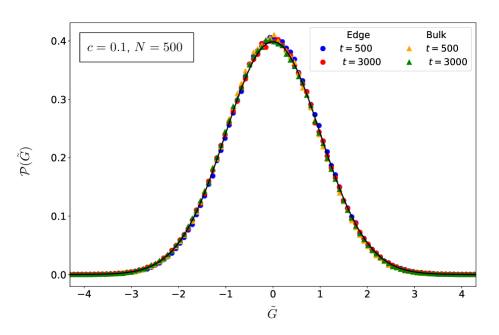
Figure 4: Plot of the distribution of the centered and scaled gap $\tilde{G}=\frac{G^{RD}-2ct}{2\sqrt{t}}$ for times $t=500$ and $t=3000$, from the numerical simulation of the Langevin equation (4) both for the mid-gap $G^{RD}\equiv G^{RD}_{\rm mid-gap}$ and for the edge gap $G^{RD}\equiv G^{RD}_{\rm edge-gap}$. Here $N=500$, $c=0.1$ (note that $c^{2}t$ is the dimensionless time). It is compared with the normal Gaussian distribution $e^{-x^{2}/2}/\sqrt{2\pi}$ as predicted in (48) and (54) (black color).

However, the behavior of the gap distribution changes as one approaches the edges of the jellium model, i.e., $g_{\rm edge-gap}=y_{N}-y_{N-1}$, has the following distribution in the large $N$ limit SatyaJellium2

$$\mathcal{P}_{\text{edge-gap}}(g) \sim N\,h_{\alpha}(gN),$$ (49)

$$h_{\alpha}(z) =\theta(z)[A(\alpha)]^{2}\int_{-\infty}^{\infty}dye^{-\frac{1}{2}[(y+z-4\alpha)^{2}+y^{2}]}F_{\alpha}(y+4\alpha),$$ (50)

where $F_{\alpha}(x)$ is the same function as defined in Eq. (41). Once again, to make correspondence with the ranked diffusion problem, we need to consider the limit $\alpha$ large. In that limit, one can again approximate this integral (50) by the saddle-point method. Following exactly the same argument as in the mid-gap case, one gets

$$\lim_{\alpha\rightarrow\infty}h_{\alpha}(z)\sim\frac{1}{\sqrt{4\pi}}e^{-\frac{1}{4}{(z-4\alpha})^{2}}\;.$$ (51)

Hence, using (49), we again get a Gaussian distribution for the edge gap in the jellium model in the large $\alpha$ limit

$$\mathcal{P}_{\text{edge-gap}}(g)\sim e^{-\frac{N^{2}}{4}(g-4\alpha/N)^{2}}\;.$$ (52)

Thus, in the large $\alpha$ limit, the edge and bulk gaps in the jellium model behave in the same way, namely

$$g_{\rm edge-gap}\approx\frac{4\alpha}{N}+\frac{\sqrt{2}}{N}{\cal N}(0,1)\;.$$ (53)

Correspondingly, the edge-gap and in the mid-gap behave in a same way, namely

$$G^{\rm RD}_{\rm edge-gap}=x_{N}(t)-x_{N-1}(t)\approx 2c\,t+2\,\sqrt{t}{\,\cal N}(0,1)\;.$$ (54)

Although this result, together with (48), was obtained here at large $N$, we note by comparing to Eq. (18) that it already holds for $N=2$ for the first two cumulants, which thus appears to independent of $N$.

In summary, the predictions (48) and (54) from the analogy with the equilibrium are in agreement with the discussion at the end of the previous subsection, i.e., that on the scale $\delta x_{i}\sim\sqrt{t}$ the fluctuations are independent Gaussian, as indeed recovered in the large $\alpha$ limit of the jellium. In Fig. 4, we verify by Monte-Carlo simulations the two analytical predictions for the gaps in the ranked diffusion model respectively in Eqs. (48) and (54). We see that the agreement is indeed excellent if the gaps are scaled by $\sqrt{t}$.

However, this is not the end of the story for the dynamics problem, and in the next subsection we will compute the higher cumulants of the particle positions $x_{i}$ at large time, which exhibit deviations from this leading Gaussian behavior.

III.4 More accurate treatment of the large time limit: higher cumulants

In this section we go back to the complete asymptotic form for the joint PDF at large time (23),(25) and we obtain all the cumulants of the particle positions $x_{i}$ to $O(1)$ accuracy.

III.4.1 The case $N=2$

Let us start with $N=2$ for simplicity. Consider the large time asymptotic formula (16). Let us recall that the original variable is $y=x_{2}-x_{1}=zt$. We can consider the sector $y>0$: indeed we will use a saddle point method, and there will be one saddle point inside each sector and the result will not depend on the sector (see below). We want to evaluate the cumulant generating function

$$\langle e^{\lambda y}\rangle=\langle e^{t\lambda z}\rangle\simeq\int_{0}^{+\infty}dze^{-\frac{t}{4}(z-2c)^{2}+\log(\frac{z}{z+2c})+f(t)+t\lambda z}$$ (55)

where we have inserted (16) and the normalization factor $f(t)=-\ln(2\sqrt{2\pi t})$ is immaterial for the following. At large $t$ there is a unique saddle point at $z=z^{*}=2c+2\lambda$. We require that $2c+2\lambda>0$ (in fact for the cumulants we only need $\lambda$ in a neighborhood of $\lambda=0$). From the saddle point method we thus obtain

$$\langle e^{\lambda y}\rangle\simeq\exp\left(2t\lambda+2\lambda^{2}t+\log\left(\frac{2c+2\lambda}{2c+\lambda}\right)\right)$$ (56)

where we have fixed the normalization so that the r.h.s. is equal to unity at $\lambda=0$. Using that $\log\langle e^{\lambda y}\rangle=\sum_{k\geq 1}\frac{\lambda^{k}}{k!}\langle y^{k}\rangle_{c}$ and expanding in $\lambda$ we obtain all the cumulants. This reproduces the results in Eqs. (17)-(20) up to and including $O(1)$ terms at large time, and gives the more general formula for $k\geq 2$

$$\langle y^{k}\rangle_{c}=\frac{1}{c^{k}}\,(-1)^{k-1}(k-1)!(2^{k}-1)+o(1)$$ (57)

Several remarks are in order. First, since (16) depends only on $|z|$, instead of choosing the sector $y>0$ we could have done the exact same calculation replacing $y$ by $|y|$, and $z$ by $|z|$. The saddle point is then at $|z|=2c+2\lambda$, so there are in fact two identical saddle points for each sign of $y$. Hence to the same accuracy $\langle(|y|-2ct)^{k}\rangle_{c}=\langle y^{k}\rangle_{c}$ given by (57). Next we see that (56) holds for any $\lambda>-c$, but fails when $\lambda\leq-c$, since for $\lambda=-c$ the saddle point reaches $z=0$. The average $\langle e^{\lambda y}\rangle$ is then dominated by the vicinity of $z=0$, i.e., by events which involve particle crossings, and the two sectors cannot be neatly separated. Finally, we know from the exact results (17)-(20) that the $o(1)$ corrections in (57) should be exponentially small $O(e^{-c^{2}t/2})$ at large time. But the above saddle-point method, if pushed to next order, will lead power law in time corrections $O(1/t^{k})$. This apparent paradox is resolved in the Appendix, where it is shown that (56) has indeed only exponentially small corrections in time. The reason for that is that (16) itself comes from a first saddle point method, and both saddle points should be considered simultaneously. In the Appendix we identify these exponentially small corrections to (56) to come precisely from particle crossing, which are exponentially rare for $c^{2}t\gg 1$.

III.4.2 The case of arbitrary $N$

Let us now turn to arbitrary $N$ and consider the sector $x_{1}<x_{2}<\dots<x_{N}$, recalling that we denote $x_{j}=tz_{j}$. Let us compute the following generating function at large time, inserting the asymptotic form (25),

$$\langle e^{\sum_{j}\lambda_{j}x_{j}}\rangle=\langle e^{t\sum_{j}\lambda_{j}z_{j}}\rangle\simeq\int_{z_{1}<z_{2}<\dots<z_{N}}dz_{1}\dots dz_{N}e^{-\frac{t}{4}\sum_{j=1}^{N}(z_{j}-c(2j-N-1))^{2}+t\sum_{j=1}^{N}\lambda_{j}z_{j}+\sum_{1\leq a<b\leq N}\log\frac{z_{b}-z_{a}}{z_{b}-z_{a}+2c}+f(t)}$$ (58)

where again $f(t)$ is an unimportant normalization. In this sector there is a unique saddle point at large $t$ given by

$$z_{j}=z_{j}^{*}=c(2j-N-1)+2\lambda_{j}\quad,\quad j=1,\dots,N$$ (59)

We will assume that the $z_{j}^{*}$ are in the sector considered, i.e., that all $c(2j-N-1)+2\lambda_{j}>0$ for $j=1,\dots,N$, which is certainly the case when the $\lambda_{j}$’s are all in a neighborhood of zero. Then the saddle point method gives

$$\langle e^{\sum_{j}\lambda_{j}x_{j}}\rangle\simeq N!\exp\left(\sum_{j=1}^{N}c(2j-N-1)t\lambda_{j}+t\sum_{j=1}^{N}\lambda_{j}^{2}+\sum_{1\leq a<b\leq N}\log(\frac{c(b-a)+\lambda_{b}-\lambda_{a}}{c+(b-a)c+\lambda_{b}-\lambda_{a}})\right)$$ (60)

where we used $\sum_{1\leq a<b\leq N}\frac{b-a}{1+b-a}=1/N!$ to normalize the formula.

Upon expanding the logarithm of (60) in the parameters $\lambda_{j}$ we can now compute all the joint cumulants of the deviations from the perfect crystal, defined as $\delta x_{j}=x_{j}-c(2j-N-1)t$. First we note that the double sum in (60) involves only pairs of distinct variables $\lambda_{j}$. Hence the cumulants involving more than two particles are zero, e.g.

$$\langle\delta x_{i}\delta x_{j}\delta x_{k}\rangle_{c}=0\quad,\quad\text{for}\quad i<j<k$$ (61)

To compute the only non-zero cumulants (i.e., involving only one or two particles) we first define the function

$$f_{k}(x)=\log\left(\frac{ck+x}{c+ck+x}\right)\;,$$ (62)

which has derivatives

$$c^{k}f_{k}^{(n)}(0)=(-1)^{n-1}(n-1)!\left(\frac{1}{k^{n}}-\frac{1}{(k+1)^{n}}\right)$$ (63)

From the logarithm of (60) we obtain the single particle cumulants as

$$\langle(\delta x_{i})^{n}\rangle_{c}=\sum_{i<j\leq N}\partial_{\lambda_{i}}^{n}f_{j-i}(\lambda_{j}-\lambda_{i})|_{\lambda_{i}=\lambda_{j}=0}+\sum_{1\leq j<i}\partial_{\lambda_{i}}^{n}f_{i-j}(\lambda_{i}-\lambda_{j})|_{\lambda_{i}=\lambda_{j}=0}+2t\delta_{n,2}$$ (64)

$$=\sum_{i<j\leq N}(-1)^{n}f_{j-i}^{(n)}(0)+\sum_{1\leq j<i}f_{i-j}^{(n)}(0)+2t\delta_{n,2}$$ (65)

This leads to, for $1\leq i\leq N$ and $n\geq 2$

$$\langle(\delta x_{i})^{n}\rangle_{c}=\frac{1}{c^{n}}(n-1)!\left(\frac{1}{(N-i+1)^{n}}-1+(-1)^{n-1}(1-\frac{1}{i^{n}})\right)+2t\delta_{n,2}$$ (66)

We see that at large $N$, for $i=O(1)$ i.e., at the left edge of the gas, one has

$$\lim_{N\to+\infty,i=O(1)}\langle(\delta x_{i})^{n}\rangle_{c}=\frac{1}{c^{n}}(n-1)!\left(-2\delta_{n,\rm even}+\frac{(-1)^{n}}{i^{n}}\right)+2t\delta_{n,2}$$ (67)

We see that in the bulk of the gas, i.e., for $i\to+\infty$, the odd cumulants decay to zero, while the even cumulants $n\geq 4$ decay from $-\frac{3}{c^{n}}(n-1)!$ for $i=1$, to a finite limit $-\frac{2}{c^{n}}(n-1)!$, which is uniform over the bulk of the gas. Hence the fluctuations are slightly larger near the edge, but remain finite in the bulk. On the right edge the result is similar, with the term $\frac{(-1)^{n}}{i^{n}}$ replaced by $\frac{1}{(N-i+1)^{n}}$.

Next, we compute the cumulants involving two particles (for $j>i$, $m,n\geq 1$ and $N\geq 2$). One finds

$$\langle\delta x_{i}^{n}\delta x_{j}^{m}\rangle_{c}=\partial_{\lambda_{i}}^{n}\partial_{\lambda_{j}}^{m}f_{j-i}(\lambda_{j}-\lambda_{i})|_{\lambda_{i}=\lambda_{j}=0}=(-1)^{n}f_{j-i}^{(n+m)}(0)$$

$$=\frac{1}{c^{n}}(-1)^{m-1}(n+m-1)!\left(\frac{1}{(j-i)^{n+m}}-\frac{1}{(j-i+1)^{n+m}}\right)$$ (68)

We note that these correlations are independent of $N$ and decay quickly to zero as a function of the distance between the two particles.

These formulae are exact for all $N$. For concreteness let us display some of the predictions for $N=2,3$. For simplicity we set here $c=1$. For $N=2$ this gives

$$\langle(\delta x_{1})^{2}\rangle_{c}=\langle(\delta x_{2})^{2}\rangle_{c}=2t-\frac{3}{4}\quad,\quad\langle\delta x_{1}\delta x_{2}\rangle_{c}=\frac{3}{4}$$ (69)

$$\langle(\delta x_{1})^{3}\rangle_{c}=-\langle(\delta x_{2})^{3}\rangle_{c}=-\frac{7}{4}\quad,\quad\langle\delta x_{1}(\delta x_{2})^{2}\rangle_{c}=-\langle(\delta x_{1})^{2}\delta x_{2}\rangle_{c}=-\frac{7}{4}$$ (70)

For $N=3$ we obtain

$$\langle\delta x_{1}\rangle=-2/3\quad,\quad\langle\delta x_{2}\rangle=0\quad,\quad\langle\delta x_{3}\rangle_{c}=2/3$$ (71)

$$\langle\delta x_{1}^{2}\rangle_{c}=\langle\delta x_{3}^{2}\rangle_{c}=2t-\frac{8}{9}\quad,\quad\langle\delta x_{2}^{2}\rangle_{c}=2t-\frac{3}{2}\quad,\quad\langle\delta x_{1}\delta x_{2}\rangle_{c}=\langle\delta x_{2}\delta x_{3}\rangle_{c}=\frac{3}{4}\quad,\quad\langle\delta x_{1}\delta x_{3}\rangle_{c}=\frac{5}{36}$$ (72)

$$\langle\delta x_{1}^{3}\rangle_{c}=-\langle\delta x_{3}^{3}\rangle_{c}=-\frac{52}{27}\quad,\quad\langle\delta x_{2}^{3}\rangle_{c}=0\quad,\quad\langle\delta x_{1}\delta x_{2}^{2}\rangle_{c}=-\langle\delta x_{1}^{2}\delta x_{2}\rangle_{c}=-\frac{7}{4}$$ (73)

$$\langle\delta x_{1}^{2}\delta x_{3}\rangle_{c}=-\langle\delta x_{1}\delta x_{3}^{2}\rangle_{c}=\frac{19}{108}\quad,\quad\langle\delta x_{2}\delta x_{3}^{2}\rangle_{c}=-\langle\delta x_{2}^{2}\delta x_{3}\rangle_{c}=-\frac{7}{4}\quad,\quad\langle\delta x_{1}\delta x_{2}\delta x_{3}\rangle_{c}=0\;.$$ (74)

Next one can use these formula to compute the cumulants of the relative distance between any two particles. Since the cumulants of $x_{j}$ and of $\delta x_{j}$ are by definition identical, we will simply use the particle positions $x_{j}$ here. For $1\leq i<j\leq N$ one finds

$$\langle(x_{j}-x_{i})^{n}\rangle_{c}=\frac{(n-1)!}{c^{n}}\bigg{(}i^{-n}+(-1)^{n}\left(2^{n}-2\right)\left((-i+j+1)^{-n}-(j-i)^{-n}\right)$$ (75)

$$+(-1)^{n}(-i+N+1)^{-n}+(-1)^{n}j^{-n}+(-j+N+1)^{-n}-2(-1)^{n}-2\bigg{)}+4t\delta_{n,2}+2t{c\,(j-i)}\delta_{n,1}\;,$$ (76)

which for $j=i+1$ gives the cumulants of the gaps, for which one finds for $1\leq i\leq N-1$

$$\langle(x_{i+1}-x_{i})^{n}\rangle_{c}=\frac{(n-1)!}{c^{n}}\bigg{(}i^{-n}+(N-i)^{-n}+(-1)^{n}(-i+N+1)^{-n}+(-1)^{n}(i+1)^{-n}$$ (77)

$${+}(-1)^{n}\left(-2^{1-n}-2^{n}+1\right)-2\bigg{)}+4t\delta_{n,2}+2c\,t\delta_{n,1}\;.$$

Again, in the large $N$ limit one finds some distinct behavior at the two edges, and that the cumulants of the gap reach a finite limit inside the bulk given by the second line of (77).

Similarly one finds that the cumulants of the total size of the gas (i.e., its span) are given by

$$\langle(x_{N}-x_{1})^{n}\rangle_{c}=(-1)^{n}\frac{(n-1)!}{c^{n}}\left(2^{n}N^{-n}{-}\left(2^{n}-2\right)(N-1)^{-n}{+}2\right)+4t\delta_{n,2}+2{c\,(N-1)}t\delta_{n,1}\;.$$ (78)

For large $N$ the $n$-th cumulant ($n>1$) of the total size of the gas converge quickly to some finite limit

$$\langle(x_{N}-x_{1})^{n}\rangle_{c}\simeq 2(-1)^{n-1}\frac{(n-1)!}{c^{n}}(1-\frac{1}{N^{n}}+\dots)+4t\delta_{n,2}+2c(N-1)\,t\delta_{n,1}\;,$$ (79)

which, at large $N$, is equivalent to the sum of independent fluctuations, $\langle(\delta x_{N})^{n}\rangle_{c}+(-1)^{n}\langle(\delta x_{1})^{n}\rangle_{c}$, since the mutual fluctuations decay at large distance as pointed out above. It is interesting that there are non Gaussian persistent correlations at large time, on the scale of the gas, even at large $N$.

To summarize we have obtained a complete quantitative picture of the $O(1)$ fluctuations at large time in the expanding crystal which goes beyond the independent Gaussian $O(\sqrt{t})$ fluctuations discussed in the previous subsections. These result are valid for $c^{2}t\gg 1$ and any $N$. From the considerations for $N=2$ (see Appendix A), we can surmise that the corrections to these cumulants, and to (60), are exponentially small at large time and related to particle crossing (hence also in part to the finite $\alpha$ physics of the equilibrium jellium).

IV Approach via the Burgers equation

Until now we have focused on taking the large time limit first, with a fixed number of particles $N$. In this section we first recall the exact hydrodynamic equation which describes the evolution of the density. Using this equation we then study the limit of large $N$ first, at arbitrary fixed time $t$. This provides a description of the dense regimes I and II discussed in the introduction. Finally, we compare the predictions with numerical simulations.

IV.1 Burgers equation and large $N$ limit

Let us first recall the general approach developed in PLDRankedDiffusion . Let us consider again the Langevin equation (4) for $N$ particles. One defines respectively the density field $\rho(x,t)$ and the rank field $r(x,t)$ as

$$\rho(x,t)=\frac{1}{N}\sum_{i}\delta(x-x_{i}(t))=\partial_{x}r(x,t)\quad,\quad r(x,t)=\int^{x}_{-\infty}dx^{\prime}\rho(x^{\prime},t)-\frac{1}{2}\;.$$ (80)

It is convenient to choose the rank field $r(x,t)$ increasing monotonically from $-1/2$ at $x=-\infty$ to $+1/2$ at $x=+\infty$. Then it is shown in PLDRankedDiffusion , using the Dean-Kawasaki method KK93 ; Dean ; Kawa , that the rank field satisfies the stochastic equation

$$\partial_{t}r(x,t)=T\partial_{x}^{2}r(x,t)-2Nc\,r(x,t)\partial_{x}r(x,t)+\frac{1}{\sqrt{N}}\sqrt{2T\partial_{x}r(x,t)}\eta(x,t)\;.$$ (81)

In the right hand side (RHS) of (81), the first term originates from diffusion, the second is a convection term where the local velocity is proportional to the local rank, while the third term is the noise, originating from local Brownian dynamics. In PLDRankedDiffusion the case of an additional external potential $V(x)$ was also considered, but here we set it to zero. Hence Eq. (81) is the Burgers equation with a multiplicative noise. Note that the function $r(x,t)$ is constrained to be increasing in $x$, so that the density remains positive. This equation is formally exact for arbitrary $N$ (with the possible mathematical caveat that $r(x,t)$ is a discontinuous stochastic function). Here we recall that we consider $c>0$.

Let us now discuss the large $N$ limit. As discussed in PLDRankedDiffusion there are a priori two natural scalings of $c$ in that limit. In both cases, the noise term is formally subdominant.

IV.2 Detailed solution for $c=\gamma/N$ and comparison with numerics

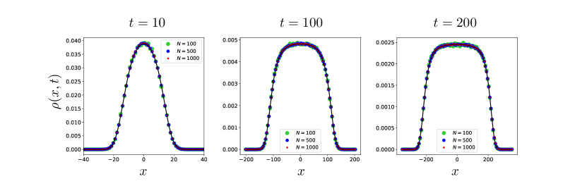
Figure 5: Plot of the density $\rho(x,t)$ evaluated numerically from the Langevin equation, at three different times $t=10,100$ and $t=200$ for $\gamma=1$ and $T=1$. The initial condition is that all particles are at the origin at time zero. For each time we simulated the density profile for three different combinations of $N$ and $c$ with fixed $\gamma=Nc=1$. The averaging is done over $10^{4}$ realizations of the noise. The numerical data is compared with the analytical prediction with a delta function initial condition from Eq. (87) (black solid lines).

(i) The first choice is to keep $c$ fixed. In that case, one defines a rescaled time $\tau=Nt$. The noise term and the diffusion term become both $O(1/N)$ and (81) simply becomes the inviscid Burgers equation, $\partial_{\tau}r=-2cr\partial_{x}r$. The solution is obtained implicitly by solving for $r\equiv r(x,t)$ equation PLDRankedDiffusion

$$r=r_{0}(x-2c\,r\tau)$$ (82)

where $r(x,0)=r_{0}(x)$ is the initial condition. Since $c>0$ there is a unique solution with no shocks. An example is the square density initial condition, $\ell>0$

$$\rho(x,t)=\frac{1}{2(\ell+c\tau)}\theta(\ell+c\tau-|x|)\quad,\quad\tau=N\,t\;,$$ (83)

which shows that the repulsive gas expands linearly in time with sharp edges at $\pm c\tau=\pm cNt$. This result (restoring $\tau=Nt$) matches with the prediction (39) which was obtained in the large time limit followed by the large $N$ limit. Note that here the convergence to the form (83) occurs quite fast, on a time scale $\tau=O(1)$ that is $t\sim 1/N$. Comparing with the discussion in the introduction, we see that this time regime corresponds to regime II where the square density forms and expands, and in the inviscid Burgers equation the edges are sharp on scale $x=O(1)$.

(ii) Here we will consider the second and richer choice of scaling, i.e., $c=\gamma/N$ where $\gamma>0$ is fixed. In that case, only the noise term is subdominant $O(1/\sqrt{N})$ in (81), and one obtains the viscous Burgers equation in the original time variable $t$, namely

$$\partial_{t}r(x,t)=T\partial_{x}^{2}r(x,t)-2\gamma\,r(x,t)\partial_{x}r(x,t)\;.$$ (84)

As we will see below, the solution of this equation with a square density initial condition (with $\ell>0$) is similar in the bulk to (83), since the first term in the RHS of (84) is essentially zero for a flat density profile. This also leads to an expansion of the gas which is linear in time with the same speed. The main difference occurs near the edges, the sharp edges of (81) at $\pm\gamma t=\pm c\,N\,t$ being replaced by a smooth profile with a boundary layer form. For attractive interactions studied in PLDRankedDiffusion there is a stationary state and the boundary layer has a width $\xi=\frac{T}{cN}=\frac{T}{\gamma}$ determined by comparing the two terms in the r.h.s. of (84). It turns out that in the case studied here, i.e., repulsive interactions and a delta initial condition for the density, the gas is always far from stationarity and we show below that the scale which determines the size of the boundary layer is the diffusion length scale $\ell_{T}=\sqrt{2Tt}$ (within the boundary layers the three terms in (84) are of the same order).

Note that the characteristic length and time scales associated with the Burgers equation (84) are $x\sim T/\gamma=T/(Nc)$ and $t\sim T/\gamma^{2}=T/(N^{2}c^{2})=t_{1}^{*}$ (which would allow to eliminate the $\gamma$ dependence in (84)). Hence this equation naturally describes the crossover between the regime I and II.

In order to compare with the numerics we give here the explicit form of the density and rank field obtained by solving analytically Eq. (84) for two cases.

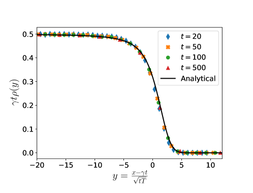
Figure 6: Comparison of numerical simulation of the boundary layer at the right edge with the result from Eq. (90). In the simulation $\gamma=cN=7$ with $N=1000$, $c=0.007$ and $T=1$. We chose four different times $t\in\{20,50,100,500\}$, which is inside regime II. The averaging is done over $10000$ realizations of the noise and at $t=0$ all particles are at $x=0$.

(i) For the initial condition corresponding to all particles initially at $x=0$, as in (9), which corresponds to $r_{0}(x)=\frac{1}{2}{\rm sgn}(x)$ one finds (e.g. using Eq. (25) in PLDRankedDiffusion )

$$r(x,t)=-\frac{T}{\gamma}\partial_{x}\log\left(f(x,t)+f(-x,t)\right)$$ (85)

$$f(x,t)=\int_{0}^{+\infty}\frac{dw}{\sqrt{4\pi Tt}}e^{-\frac{(w-x)^{2}}{4Tt}-\frac{\gamma}{T}\frac{w}{2}}=\frac{1}{2}e^{\frac{1}{4T}\gamma(\gamma t-2x)}\text{erfc}\left(\frac{\gamma t-x}{2\sqrt{Tt}}\right)\;.$$ (86)

This leads to the time dependent density

$$\rho(x,t)=\partial_{x}r(x,t)=\frac{e^{-\frac{(x-\gamma t)^{2}}{4tT}}\left(\frac{e^{\frac{\gamma x}{T}}\text{erfc}\left(\frac{\gamma t+x}{2\sqrt{t}\sqrt{T}}\right)}{\sqrt{t}\sqrt{T}}+\text{erfc}\left(\frac{\gamma t-x}{2\sqrt{t}\sqrt{T}}\right)\left(\frac{1}{\sqrt{t}\sqrt{T}}-\frac{\sqrt{\pi}\gamma e^{\frac{(\gamma t+x)^{2}}{4tT}}\text{erfc}\left(\frac{\gamma t+x}{2\sqrt{t}\sqrt{T}}\right)}{T}\right)\right)}{\sqrt{\pi}\left(\text{erfc}\left(\frac{\gamma t-x}{2\sqrt{t}\sqrt{T}}\right)+e^{\frac{\gamma x}{T}}\text{erfc}\left(\frac{\gamma t+x}{2\sqrt{t}\sqrt{T}}\right)\right)^{2}}\;.$$ (87)

(ii) For a box shape initial density of width $2\ell$, i.e., $\rho(x,0)=\frac{1}{2\ell}\theta(\ell-|x|)$, the solution is given by (see Eqs. (171)-(172) in PLDRankedDiffusion ), where one sets $T=1$

$$\rho(x,t)=\partial_{x}r(x,t)\quad,\quad r(x,t)=-\frac{1}{\gamma}\partial_{x}\log\left(f(x,t)+f(-x,t)\right)$$ (88)

$$f(x,t)=\frac{e^{-\frac{\gamma x^{2}}{4({\ell}+\gamma t)}}}{\sqrt{1+\frac{\gamma t}{{\ell}}}}\text{erf}\left(\frac{{\ell}+\gamma t+x}{2\sqrt{t}\sqrt{1+\frac{\gamma t}{{\ell}}}}\right)+e^{\frac{1}{4}\gamma({\ell}+\gamma t+2x)}\text{erfc}\left(\frac{{\ell}+\gamma t+x}{2\sqrt{t}}\right)\;.$$ (89)

For $\ell\to 0$ this formula gives back the result (88) for the delta initial condition.

The analytical formula (87) for the density, with a delta initial condition, is plotted in Fig. 5 for several values of $t$ (solid line). We see that in the limit of large time $t\gg\frac{1}{\gamma^{2}}$ the density predicted by the Burgers equation evolves towards a flat profile for $x\in[-\gamma t,\gamma t]$. In addition, as can be seen on the figure, there is a boundary layer at each edge. From (87) one can derive the precise form of this boundary layer (see Appendix C) and one finds that the density near the right edge at $x=\gamma t$ takes the form

$$\rho(x,t)=\frac{1}{\gamma t}\hat{\rho}\left(\frac{x-\gamma t}{\sqrt{Tt}}\right)\quad,\quad\hat{\rho}(y)=\frac{e^{-\frac{y^{2}}{2}}\left(2+\sqrt{\pi}e^{\frac{y^{2}}{4}}y\,\text{erfc}\left(-\frac{y}{2}\right)\right)}{2\pi\text{erfc}\left(-\frac{y}{2}\right)^{2}}\;.$$ (90)

The characteristic width is thus the diffusion length $\ell_{T}=\sqrt{Tt}$, see (1). As mentioned above, here $t=O(T/\gamma^{2})=O(T/(cN)^{2})$, hence this width is itself of order $T/(cN)$. The scaling function has the asymptotic behavior $\hat{\rho}(y)\simeq\frac{1}{2}-\frac{1}{y^{2}}$ for $y\to-\infty$, which thus matches the density of the plateau $\rho(x,t)\simeq\frac{1}{2\gamma t}=\frac{1}{2cNt}$. On the other side it has a fast decay, $\hat{\rho}(y)=\frac{y}{2\sqrt{\pi}}e^{-\frac{y^{2}}{4}}$ for $y\to+\infty$.

We have plotted the prediction (90) in Fig. 6 (solid line) where it is also compared with numerical simulations for various times inside regime II (see below). We see that the agreement of the data with the scaling function is excellent.

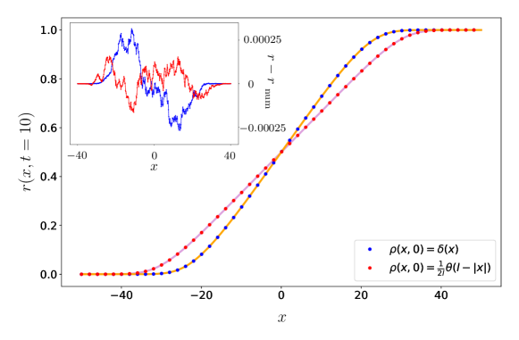
Figure 7: The rank field $r(x,t)$ computed numerically (dots) and from the analytical expression (full lines) for two different initial conditions. Red colored dots represent the square initial condition $\rho(x,0)=\frac{1}{2l}\theta(l-|x|)$ for $l=10$. The numerical data are compared with the analytical expression in Eq. (88) (solid purple line). The blue colored dots shows the numerical data for the initial condition where all the particles start from the origin. The analytical expression from Eq. (85) is represented by orange solid line. Inset: point-wise difference between numerical data, $r_{\rm num}(x,t)$, and the analytical expression $r(x,t)$ for both delta and square initial conditions. The deviations are of order $10^{-3}$. For both plots the rank field is measured at $t=10$ with $\gamma=2$, $T=1$, and $N=1000$. Here the data are averaged over $10^{3}$ different realizations, which shows a small systematic deviation, due to the finite $N$ effects (see Fig. 8).

In the opposite limit $t\ll\frac{1}{\gamma^{2}}$ one can check that formula (87) converges to the Gaussian profile for independent diffusing particles $\rho(x,t)\simeq\frac{1}{\sqrt{4\pi Tt}}e^{-x^{2}/(4Tt)}$.

We now compare these predictions with a direct numerical calculation of the trajectories $x_{j}(t)$ from the Langevin equations (4) where we set $T=1$ and $c=\gamma/N$. In Fig. 5 we study the case where all the particles start from the origin at $t=0$. We plot the numerically evaluated density $\rho(x,t)$ as a function of $x$ for different times $t$ (and several values of $N$), averaged over $10^{4}$ realizations of the noise. This is compared with the prediction in Eq. (87) with an initial delta function density. We see that the agreement is quite good, hence in this time regime the density is very well described by the deterministic Burgers equation even for moderate values of $N$.

The matching between the solution derived from the Burgers equation and the numerical simulations can be further investigated by looking at the rank fields. In Fig. 7 we present the numerical evaluation of the rank fields for $N=1000$ for both the square and the delta initial conditions for $t=50$ and $\gamma=2$. In the inset, we have plotted the difference between the observed and predicted values of the rank field as a function of $x$, as given in (88) and (87). One can see that these differences are quite small.

Next we study how these differences between the observed and the predicted values of the rank field behave as a function of $N$ and the time $t$, for both initial conditions. For this purpose, we define the error $\Sigma$ as

$$\Sigma(N,t)=\sqrt{\frac{1}{n}\sum_{\alpha=1}^{n}(r(y_{\alpha},t)-{r}_{\rm num}(y_{\alpha},t))^{2}}\;,$$ (91)

where $n$ is the number of points on a grid $\{y_{\alpha}\}$ at which we numerically computed the rank field (typically $500\leq n\leq 2000$), $r(y_{\alpha},t)$ is the predicted rank field at those points and ${r}_{\rm num}(y_{\alpha})$ is the numerical rank field at $y_{\alpha}$.

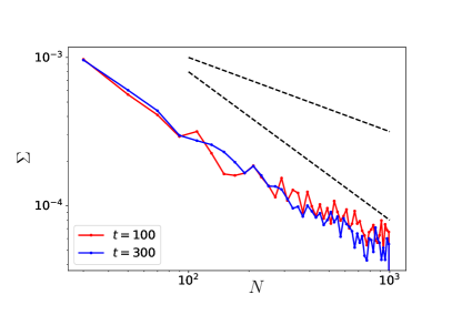
Figure 8: Fluctuations of the rank field as measured by $\Sigma(N,t)$ defined in (91). We plotted the numerical data for $\Sigma$ as a function of $N$ in log-log scale for $n=500$ and two different times $t=100$ and $t=300$. We have checked that the number of points $n$ on the grid [see Eq. (91)], does not affect significantly the data. Here we fixed $\gamma=1$, $T=1$, and we averaged over $10^{4}$ realizations of the noise. At time zero we start from the square initial condition with $l=10$. The dashed lines are guides to the eyes and have slopes respectively $-1/2$ and $-1$.

In the left panel of Fig. 8, we have plotted $\Sigma(N,t)$, on a log-log scale, as a function of $N$ for different initial profiles at different times. For the square initial condition with $\ell=10$, we see that $\Sigma(N,t)$ decays with $N$ as a power law $N^{-a}$, where we measure $1/2<a<1$.

V Conclusion

In this paper we have studied the out of equilibrium Langevin dynamics of $N$ particles in one dimension, which interact only via the linear $1d$ repulsive Coulomb potential, and which are thus allowed to cross. We have focused on an initial condition where all the particles are at the origin at time $t=0$. As time increases the gas expands. We have shown that there are three distinct regimes in time, separated by two characterictic times. In regime I, i.e., $t<t_{1}^{*}=T/(cN)^{2}$ the particles perform essentially independent Brownian diffusion. At $t=t_{1}^{*}$, the particles start feeling the long-range interaction and for $t>t_{1}^{*}$ the size of the gas increases linearly $\sim 2cNt$, this is the beginning of regime II. A plateau forms in the particle density, with boundary layers of size $\sqrt{2Tt}$ whose shape we have explicitly computed using a relation with the Burgers equation. In this regime II the gas is still dense and the particles still experience many mutual crossings. Finally as $t\geq t_{2}^{*}=T/c^{2}$ one enters the regime III where the system is a dilute expanding crystal where the particles are well separated. We have studied the regime III at large time thanks to an exact formula obtained from the Bethe ansatz which we analyzed using a saddle point method. The time dependent particle distribution shows a remarkable analogy with the one that describes the equilibrium jellium model in the presence of a quadratic well with a time dependent curvature. This allows to quantify the fluctuations of the displacements in the expanding crystal, which are Gaussian and of order $O(\sqrt{t})$ to leading order. Interestingly there are additional $O(1)$ subleading non-Gaussian fluctuations which we obtain exactly. These additional correlations are purely dynamical in origin and do not have any counterpart in the equilibrium jellium model.

There are many interesting questions which remain to be studied. One is the role of the initial conditions. Presumably, in the regime III, the analogy with the equilibrium jellium model and the leading Gaussian fluctuations are a robust features. However it is likely that the subleading $O(1)$ non-Gaussian fluctuations for $t\gg T/c^{2}$ depend on some details of the initial condition. Indeed we have shown that it is the case for $N=2$, see Appendix A.4 where the few lowest cumulants are obtained explicitly for any even initial condition. This shows that the system keeps some memory of the initial condition even at infinite time. It remains to be investigated how this feature extends to any $N$, and whether it persists at large $N$. Another interesting open question is to describe the crossover from regime II to regime III, i.e., times of order $t_{2}^{*}=T/c^{2}$ or smaller. Indeed, as we have shown, the crossover from regime I to regime II for times of order $T/(cN)^{2}$ can be described using an hydrodynamic approach based on the Burgers equation. This approach however fails as time increases around $t=t_{2}^{*}$ when one cannot neglect anymore the discreteness of the particles. In particular we expect that the boundary layer at the edges of the plateau in the density becomes quite different from the one computed here. Describing the system in that regime remains an open challenge.

The stochastic dynamics of long-range interacting systems with a non-equilibrium stationary state, such as the Hamiltonian mean-field model, has been studied in the past Gupta1 ; Gupta2 . In contrast, our work concerns the dynamics in a long-range interacting system where there is no stationary state. In the present study we have obtained new results in the broader context of interacting Brownian particles with long range interactions by a combination of analytical methods. A general model much studied recently, in mathematics and physics, mostly at equilibrium Lewin ; Agarwal_riesz ; Beenakker_riesz , or its quantum generalization Huse_riesz is the so-called Riesz gas in one dimension where the repulsive interaction potential behaves as a power law of the distance $\sim|x_{i}-x_{j}|^{-s}$. The case $s=-1$ corresponds to the Coulomb interaction studied here, and the case $s=0$ is the log-gas. The out of equilibrium dynamics for general $s$ has not been much addressed (apart of course from $s=0$ and the Dyson’s Brownian motion mehta_book ) with the exception of a very recent work Mallick_riesz , where the case $s>0$ was studied using hydrodynamics methods. The present work opens the way for further investigations of non-equilibrium dynamics for Brownian particle systems with long range interactions.

Appendix A More details for two particles $N=2$

A.1 Solution from Laplace transform

For two particles one can solve directly the problem in Laplace (as in Supp. Mat. of PLDRankedDiffusion but for $c>0$). Noting $x(t)=\frac{1}{2}(x_{1}(t)+x_{2}(t))$ and $y(t)=x_{2}(t)-x_{1}(t)$, the center of mass performs an independent unit Brownian motion, $\dot{x}(t)=\xi(t)$, while the relative coordinate evolves as

$$\dot{y}=2c\,{\rm sgn}(y)+2\eta(t)\;,$$ (92)

where $\eta(t)$ is an independent unit white noise. Its probability density $P(y,t)$ then evolves according to

$$\partial_{t}P=2\partial_{y}^{2}P-2c\partial_{y}({\rm sgn}(y)P)\;.$$ (93)

starting with the initial condition $P(y,0)=\delta(y)$. Introducing the Laplace transform $\tilde{P}(y,s)=\int_{0}^{+\infty}dte^{-st}P(y,t)$ one obtains

$$s\tilde{P}-P(y,0)=2\partial_{y}^{2}\tilde{P}-2c\partial_{y}({\rm sgn}(y)\tilde{P})\;,$$ (94)

where $P(y,0)$ is the initial condition. It is then easy to solve separately for $y>0$ and $y<0$. There are two integration constants on both sides. One on each side is set to zero by requiring that $\tilde{P}(y,s)\to 0$ at $y\to\pm\infty$ for $s>0$. Continuity of $P$ at $y=0$ gives another condition and finally, from integrating (93) on a small interval around $y=0$ one obtains the matching condition

$$P^{\prime}(0^{+},t)-P^{\prime}(0^{-},t)-2cP(0,t)=-\frac{1}{2}$$ (95)

and the same relation holds for the Laplace transforms. This leads to the unique solution

$$\tilde{P}(y,s)=\frac{e^{\frac{c}{2}|y|}}{2(c+\sqrt{c^{2}+2s})}e^{-\frac{1}{2}\sqrt{c^{2}+2s}|y|}\;.$$ (96)

Hence

$$P(y,t)=e^{-\frac{c^{2}}{2}t}e^{\frac{c}{2}|y|}{\rm LT}^{-1}_{s\to t}\frac{1}{2(c+\sqrt{2s})}e^{-\frac{1}{2}\sqrt{2s}|y|}\;.$$ (97)

Note that the prefactor $e^{-\frac{c^{2}}{2}t}e^{\frac{c}{2}|y|}$ is exactly the one which appears in the LL method setting $N=2$. Inverting explicitly the Laplace transform, one finds the formula (14) given in the text.

A.2 Comparison with the general $N$ formula

Let us rewrite the general formula (12) for $N=2$, denoting $y=x_{2}-x_{1}$ and $x=\frac{x_{1}+x_{2}}{2}$, i.e., $x_{2}=x+y/2$ and $x_{1}=x-y/2$ as above (with $dx_{1}dx_{2}=dxdy$). It reads for $x_{1}\leq x_{2}$, that is for $y\geq 0$

$$P(x_{1},x_{2},t)=e^{\frac{c}{2}|y|}e^{-\frac{c^{2}}{2}t}\int_{\mathbb{R}}\frac{dk_{1}}{2\pi}\int_{\mathbb{R}}\frac{dk_{2}}{2\pi}\frac{ik_{1}-ik_{2}}{ik_{1}-ik_{2}+c}\,e^{-t(k_{1}^{2}+k_{2}^{2})+ix(k_{1}+k_{2})+\frac{i}{2}y(k_{2}-k_{1})}$$ (98)

Let us denote $k_{1}+k_{2}=k$ and $q=(k_{2}-k_{1})/2$. The above expression factorizes and one obtains

$$P(x_{1},x_{2},t)=e^{\frac{c}{2}|y|}e^{-\frac{c^{2}}{2}t}\left(\int_{\mathbb{R}}\frac{dk}{2\pi}e^{-t\frac{k^{2}}{2}+ixk}\right)\times\left(\int_{\mathbb{R}}\frac{dq}{2\pi}\frac{-i2q}{-i2q+c}\,e^{-2tq^{2}+iyq}\right)$$ (99)

Hence the center of mass motion decouples and one has

$$P(x_{1},x_{2},t)dx_{1}dx_{2}=\frac{1}{\sqrt{2\pi t}}e^{-\frac{x^{2}}{2t}}P(y,t)dxdy$$ (100)

with for $y\geq 0$

$$P(y,t)=e^{\frac{c}{2}|y|}e^{-\frac{c^{2}}{2}t}\int_{\mathbb{R}}\frac{dq}{2\pi}\frac{-i2q}{-i2q+c}\,e^{-2tq^{2}+iyq}$$ (101)

The Laplace transform of this expression w.r.t. time $t$ reads

$$\tilde{P}(y,s)=e^{\frac{c}{2}|y|}\int_{\mathbb{R}}\frac{dq}{2\pi}\frac{-i2q}{-i2q+c}\,\frac{1}{s+2q^{2}+\frac{c^{2}}{2}}e^{iyq}$$ (102)

One has $s+2q^{2}+\frac{c^{2}}{2}=2(q-q_{+})(q-q_{-})$ with $q_{\pm}=\pm\frac{i}{2}\sqrt{2s+c^{2}}$. Since here $y>0$ we must close the contour in the upper half-plane. The pole at $q=-ic/2$ thus does not contribute, and the pole at $q=q_{+}$ contributes. We obtain from its residue

$$\tilde{P}(y,s)=ie^{\frac{c}{2}|y|}\frac{1}{2(c+\sqrt{2s+c^{2}})}\frac{-2iq_{+}}{(q_{+}-q_{-})}e^{-\frac{y}{2}\sqrt{2s+c^{2}}}=e^{\frac{c}{2}|y|}\frac{1}{2(c+\sqrt{2s+c^{2}})}e^{-\frac{y}{2}\sqrt{2s+c^{2}}}$$ (103)

which, using that the final result must be even in $|y|$ recovers the previous result, see (13) and (96).

A.3 Cumulants of $|y|-2ct$

To obtain the cumulants of $|y|-2ct$, one can compute the Laplace transform of the generating function

$$\int_{0}^{+\infty}dt\int dyP(y,t)e^{\lambda(|y|-2ct)-st}=\int dy\tilde{P}(y,s+2c\lambda)e^{\lambda|y|}$$ (104)

Using the expression (13), expanding in $\lambda$ and performing the Laplace inversion, we find the moments, and taking the logarithm we obtain the cumulants. From now on we set $c=1$ for simplicity and will restore it in the text. One obtains

$$\langle|y|\rangle-2t=(t+1)\text{erf}\left(\frac{\sqrt{t}}{\sqrt{2}}\right)-t+\sqrt{\frac{2}{\pi}}e^{-t/2}\sqrt{t}=1+O(t^{-3/2}e^{-t/2})$$ (105)

$$\langle(|y|-2t)^{2}\rangle=2\left(t^{2}+1\right)\text{erfc}\left(\frac{\sqrt{t}}{\sqrt{2}}\right)-2\sqrt{\frac{2}{\pi}}e^{-t/2}\sqrt{t}(t-1)+4t-2=4t-2+O(t^{-1/2}e^{-t/2})$$ (106)

$$\langle(|y|-2t)^{3}\rangle=12t+6+O(t^{1/2}e^{-t/2})$$ (107)

$$\langle(|y|-2t)^{4}\rangle=48t^{2}-48t-24+O(t^{3/2}e^{-t/2})$$ (108)

$$\langle(|y|-2t)^{5}\rangle=240\,t^{2}+240\,t+120+o(1)$$ (109)

$$\langle(|y|-2t)^{6}\rangle=960\,t^{3}-1440t^{2}-1440t-720+o(1)\;,$$ (110)

The first four cumulants are given in the text, and we further obtain by this method the next two cumulants

$$\langle(|y|-2ct)^{5}\rangle_{c}\simeq 744+o(1)\quad,\quad\langle(|y|-2ct)^{6}\rangle_{c}\simeq-7560+o(1)\;.$$ (111)

where here and above the terms $o(1)$ are exponentially small corrections in $t$. We see that although the moments are polynomial in $t$ the cumulants are simply $O(1)$. Furthermore, there are no power law corrections of the type $1/t^{p}$, $p\geq 1$, to either moments or cumulants. Finally, one can check that the cumulants obtained exactly here up to order $6$ agree with the general prediction obtained in Section III.4 for $k\geq 3$ (restoring $c$)

$$\langle(|y|-2ct)^{k}\rangle_{c}=\frac{1}{c^{k}}\,(-1)^{k-1}(k-1)!(2^{k}-1)+o(1)\;.$$ (112)

A.4 More general initial conditions

In the Supp. Mat. of PLDRankedDiffusion the solution for $P(y,t)$ for $N=2$ was obtained for a more general class of initial conditions. The calculation was performed for $c<0$ (i.e., setting $c=-1$), here we adapt it for $c>0$, following the same steps.

One considers an initial condition $P(y,0)$ which is smooth around $y=0$ (for convenience) and an even function of $y$. Then $P(y,t)$ is also smooth around $y=0$ and an even function of $y$. One again defines the Laplace transform with respect to time (w.r.t.), $\tilde{P}(y,s)=\int_{0}^{+\infty}dte^{-st}P(y,t)$, and one also defines the half-sided Laplace transform w.r.t. space, $\hat{P}(\mu,s)=\int_{0}^{+\infty}dy\,e^{-\mu y}\tilde{P}(y,s)$ (thus using $\lambda=-\mu$ as compared to the notations used in the previous section). One also denotes $P_{0}(\mu)=\int_{0}^{+\infty}dy\,e^{-\mu y}P(y,0)$, the half-sided Laplace transform of the initial condition. The normalization condition on the half-space implies that $P_{0}(0)=1/2$ and $\hat{P}(0,s)=\frac{1}{2s}$. Taking the double Laplace transform of Eq. (94) w.r.t. $x$ and $t$ then leads to

$$s\hat{P}(\mu,s)-P_{0}(\mu)=2\mu(\mu-c)\hat{P}(\mu,s)-2\tilde{P}^{\prime}(0,s)-2(\mu-c)P(0,s)\;.$$ (113)

Integrating (113) around $y=0$ leads to the jump conditions $P^{\prime}(0^{+},s)-cP(0^{+},s)=0$ and its solution reads

$$\hat{P}(\mu,s)=\frac{P_{0}(\mu)-2\mu\tilde{P}(0,s)}{s-2\mu(\mu-c)}\;.$$ (114)

We will use the same condition as was used for $c=-1$ in PLDRankedDiffusion to determine the unknown function $\tilde{P}(0,s)$, namely that the residue of the pole at $s=2\mu(\mu-c)$ should vanish. Indeed, for $\mu>c$, $2\mu(\mu-c)>0$ and a pole at $s>0$ would lead to a growing exponential in time, which is excluded. Hence one has

$$\tilde{P}(0,s=2\mu(\mu-c))=\frac{P_{0}(\mu)}{2\mu}\;.$$ (115)

Equivalently, setting $\mu=\mu_{s}=\frac{1}{2}(c+\sqrt{c^{2}+2s})$ (the positive root) one must have

$$\tilde{P}(0,s)=\frac{P_{0}(\mu_{s}=\frac{1}{2}(c+\sqrt{c^{2}+2s}))}{c+\sqrt{c^{2}+2s}}$$ (116)

The solution is thus

$$\hat{P}(\mu,s)=\frac{1}{s-2\mu(\mu-c)}\left(P_{0}(\mu)-2\mu\frac{P_{0}(\frac{1}{2}(c+\sqrt{c^{2}+2s}))}{1+\sqrt{c^{2}+2s}}\right)\;.$$ (117)

Let us now compute the cumulants of $|y|-2ct$. We again use the Laplace transform in time of the cumulant generating function

$$\int_{0}^{+\infty}dt\int_{-\infty}^{+\infty}dyP(y,t)e^{-\mu(|y|-2ct)-st}=\int_{-\infty}^{+\infty}dy\,\tilde{P}(y,s-2c\mu)e^{-\mu|y|}=2\hat{P}(\mu,s-2c\mu)\;.$$ (118)

Let us set from now on $c=1$ (which means lengths are in units of $1/c$ and time of $1/c^{2}$). Let us denote $m_{k}(t)=\langle(|y|-2ct)^{k}\rangle$ the moments and $\tilde{m}_{k}(s)$ their Laplace transform in time, and $\kappa_{k}(t)$ the cumulants. One has

$$\tilde{m}_{k}(s)=2(-1)^{k}\partial_{\mu}^{k}|_{\mu=0}\hat{P}(\mu,s-2\mu)\;.$$ (119)

To extract the large time behavior we perform the small $s$ expansion for each moment. For instance one finds

$$\tilde{m}_{1}(s)=\frac{2}{s}(\hat{P}_{0}(1)-\hat{P}_{0}^{\prime}(0))+\hat{P}_{0}^{\prime}(1)-\hat{P}_{0}(1)+O(s)\;,$$ (120)

which implies that

$$m_{1}(t)=2(\hat{P}_{0}(1)-\hat{P}_{0}^{\prime}(0))+f_{1}(t)\quad,\quad\int_{0}^{+\infty}dt\,f_{1}(t)=\hat{P}_{0}^{\prime}(1)-\hat{P}_{0}(1)\;,$$ (121)

where $f_{1}(t)$ decays to zero at infinity. Hence the $O(1)$ constant in the first cumulant reads

$$\kappa_{1}(t=+\infty)=2(\hat{P}_{0}(1)-\hat{P}_{0}^{\prime}(0))=\langle y+e^{-y}\rangle_{0}$$ (122)

where $\langle\dots\rangle_{0}$ means the average with respect to the initial condition $P(y,0)$. One recovers $\kappa_{1}(t=+\infty)=1$ in the limit where $P(y,0)=\delta(y)$. We see that $\kappa_{1}(t=+\infty)$ depend on the initial condition. Next one obtains

$$\tilde{m}_{2}(s)=\frac{4}{s^{2}}+\frac{2}{s}\left(2\hat{P}_{0}^{\prime}(1)+\hat{P}_{0}^{\prime\prime}(0)-2\hat{P}_{0}(1)\right)+O(s^{0})$$ (123)

which leads to

$$m_{2}(t)=4t+\langle y^{2}-2(1+y)e^{-y}\rangle_{0}+o(t)\;.$$ (124)

Thus we find that the $O(1)$ constant in the second cumulant $\kappa_{2}(t)=4t+\tilde{\kappa}_{2}(t)$ reads

$$\tilde{\kappa}_{2}(t=+\infty)=\langle y^{2}-2(1+y)e^{-y}\rangle_{0}-\langle y+e^{-y}\rangle_{0}^{2}$$ (125)

and one recovers $\tilde{\kappa}_{2}(t=+\infty)=-3$ in the limit where $P(y,0)=\delta(y)$. The third and fourth moments are

$$m_{3}(t)=12t\,\langle y+e^{-y}\rangle_{0}+\langle y^{3}+3e^{-y}\left(y^{2}+2y+2\right)\rangle_{0}+o(t)$$ (126)

$$m_{4}(t)=48t^{2}+24t\langle y^{2}-2e^{-y}(y+1)\rangle+\langle y^{4}-4e^{-y}\left(y^{3}+3y^{2}+6y+6\right)\rangle+o(t)$$ (127)

from which one obtains the third and fourth cumulants, which have heavy expressions not displayed here. One checks that all positive orders in $t$ cancel in the $k$-th cumulant, $k\geq 3$, which thus goes to a $O(1)$ constant, $\kappa_{k}(t=+\infty)$, as large time. These $O(1)$ constants carry information, up to infinite time, about some details of the initial condition.

Appendix B More on the cumulants from the saddle point

The saddle point method used in Section III.4 would predict power law in time corrections to the cumulants, but already for $N=2$ we know that these do not exist. Let us focus on $N=2$. To understand this apparent paradox, let us go one step back and start again from the formula (101) (setting $c=1$ for simplicity here)

$$\langle e^{\lambda y}\rangle=2\int_{0}^{+\infty}dye^{(\lambda+\frac{1}{2})y}e^{-\frac{1}{2}t}\int_{\mathbb{R}}\frac{dq}{2\pi}\frac{-i2q}{-i2q+1}\,e^{-2tq^{2}+iyq}$$ (128)

Instead of performing the saddle point on $q$ and then perform the saddle point on the resulting expression (as we did in Section III.4), let us simply rewrite (101) using the shifted variables $y=2t(1+2\lambda)+\hat{y}$ and $q=\frac{i}{2}(1+2\lambda)+\hat{q}$. One obtains

$$\langle e^{\lambda y}\rangle=2\int_{-{2}t(1+2\lambda)}^{+\infty}d\hat{y}\int_{\mathbb{R}}\frac{d\hat{q}}{2\pi}\frac{1+2\lambda-2i\hat{q}}{2+2\lambda-2i\hat{q}}e^{2\lambda t+2\lambda^{2}t-2t\hat{q}^{2}+i\hat{y}\hat{q}}$$ (129)

Note that the integration contour of $\hat{q}$ was $\mathbb{R}-\frac{i}{2}(1+2\lambda)$ but we brought it back to $\mathbb{R}$ since the pole at $q=-i/2$ is not crossed along the way (provided $1+2\lambda>0$). Note that this formula is exact, no saddle point has been made. Now we split the integral over $\hat{y}$ in two pieces, i.e., we write $\int_{-2t(1+2\lambda)}^{+\infty}d\hat{y}=\int_{-\infty}^{+\infty}d\hat{y}-\int_{-\infty}^{-2t(1+2\lambda)}d\hat{y}$. In the first piece we use $\int_{-\infty}^{+\infty}d\hat{y}e^{i\hat{y}\hat{q}}=2\pi\delta(q)$ and we obtain (formally the second piece corresponds to $y<0$ in (128))

$$\langle e^{\lambda y}\rangle=e^{2\lambda t+2\lambda^{2}t}\left(\frac{1+2\lambda}{1+\lambda}-2\int_{-\infty}^{-2t(1+2\lambda)}d\hat{y}\int_{\mathbb{R}}\frac{d\hat{q}}{2\pi}\frac{1+2\lambda-2i\hat{q}}{2+2\lambda-2i\hat{q}}e^{-2t\hat{q}^{2}+i\hat{y}\hat{q}}\right)$$ (130)

The idea is that the second piece is exponentially small at large time. For instance for $-2t(2+2\lambda)<\hat{y}<-2t(1+2\lambda)$ one can evaluate the integral over $\hat{q}$ by a saddle point method, with a saddle point at $\hat{q}=i\frac{\hat{y}}{4t}$. This leads to

$$\int_{\mathbb{R}}\frac{d\hat{q}}{2\pi}\frac{1+2\lambda-2i\hat{q}}{2+2\lambda-2i\hat{q}}e^{-2t\hat{q}^{2}+i\hat{y}\hat{q}}\simeq\frac{1}{\sqrt{8\pi t}}e^{-\frac{\hat{y}^{2}}{8t}}\frac{1+2\lambda+\frac{\hat{y}}{2t}}{2+2\lambda+\frac{\hat{y}}{2t}}$$ (131)

A similar estimate can be obtained for $\hat{y}<-2t(2+2\lambda)$. Hence the final integral over $\hat{y}$ is dominated by its upper bound and is thus of order $e^{-\frac{t}{2}(1+2\lambda)^{2}}$ with algebraic prefactors. This gives an exponentially small correction to the cumulants, of order $e^{-\frac{c^{2}t}{2}}$ (restoring $c$), which is indeed what is obtained by an exact calculation. Note that the exponentially small correction term in (130) comes from trajectories which cross each other, which become subdominant for $c^{2}t\gg 1$. Finally, these calculations can be generalized to any $N$, although we will display it here.

Appendix C Asymptotic behavior of the solution of Burger’s equation

To study the boundary layer of the density $\rho(x,t)$ in (87) near its right edge, let us recall some useful formulae for the delta initial condition, namely

$$r(x,t)=-\frac{T}{\gamma}\partial_{x}\log\left(f(x,t)+f(-x,t)\right)\quad,\quad f(x,t)=e^{-\frac{\gamma x}{2T}}\text{erfc}\left(\frac{\gamma t-x}{2\sqrt{Tt}}\right)\;,$$ (132)

which we have slightly simplified. Let us focus near the right edge at $x=\gamma t$, and set $x=\gamma t+y\sqrt{Tt}$. Then we find

$$f(x,t)=e^{-\frac{\gamma^{2}t}{2T}-\frac{\gamma y\sqrt{t}}{2\sqrt{T}}}{\rm erfc}(-\frac{y}{2})$$ (133)

$$f(-x,t)=e^{-\frac{\gamma^{2}t}{2T}-\frac{\gamma y\sqrt{t}}{2\sqrt{T}}}e^{-\frac{y^{2}}{4}}\frac{\sqrt{T}}{\gamma\sqrt{\pi t}}\left(1-\frac{y\sqrt{T}}{2\gamma\sqrt{t}}+O(\frac{1}{t})\right)\;.$$ (134)

Hence for $t\gg T/\gamma^{2}=T/(cN)^{2}$ and $y=O(1)$ we see that the first term dominates. Hence in that limit one has

$$r(x,t)=\frac{1}{2}-\frac{\sqrt{T}}{\gamma\sqrt{t}}\partial_{y}\log\left({\rm erfc}(-\frac{y}{2})\right)=\frac{1}{2}-\frac{\sqrt{T}}{\gamma\sqrt{t}}\hat{r}(y)\quad,\quad\hat{r}(y)=\frac{e^{-\frac{y^{2}}{4}}}{\sqrt{\pi}\text{erfc}\left(-\frac{y}{2}\right)}$$ (135)

which describes the boundary layer at the right edge. It behaves as $\hat{r}(y)\simeq\frac{y}{2}+\frac{1}{y}$ for $y\to-\infty$, hence matches the linear behavior of the plateau. The density at the edge thus takes the following boundary layer form

$$\rho(x,t)=\frac{1}{\gamma t}\hat{\rho}(\frac{x-\gamma t}{\sqrt{Tt}})\quad,\quad\hat{\rho}(y)=\frac{e^{-\frac{y^{2}}{2}}\left(2+\sqrt{\pi}e^{\frac{y^{2}}{4}}y\,\text{erfc}\left(-\frac{y}{2}\right)\right)}{2\pi\text{erfc}\left(-\frac{y}{2}\right)^{2}}$$ (136)

where the scaling function has the asymptotic behaviors

$$\hat{\rho}(y)=\frac{1}{2}-\frac{1}{y^{2}}+O(\frac{1}{y^{4}})\quad,\quad y\to-\infty$$ (137)

$$\hat{\rho}(y)=\frac{y}{2\sqrt{\pi}}e^{-\frac{y^{2}}{4}}\quad,\quad y\to+\infty$$ (138)

The boundary layer form of the density thus matches the density of the plateau $\rho(x,t)\simeq\frac{1}{2\gamma t}=\frac{1}{2cNt}$.

References

- (1) G. B. Rybicki, Exact statistical mechanics of a one-dimensional self-gravitating system, Astrophys. Space Sci. 14, 56 (1971).
- (2) P. H. Chavanis, C. Sire, Anomalous diffusion and collapse of self-gravitating Langevin particles in dimensions, Phys. Rev. E 69, 016116 (2004).
- (3) P. Kumar, B. N. Miller, D. Pirjol, Thermodynamics of a one-dimensional self-gravitating gas with periodic boundary conditions, Phys. Rev. E 95, 022116 (2017).
- (4) A. Lenard, Exact statistical mechanics of a one‐dimensional system with Coulomb forces, J. Math. Phys. 2, 682 (1961).
- (5) S. Prager, The One-Dimensional Plasma, Adv. Chem. Phys. 4, 201 (1962).
- (6) R. J. Baxter, Statistical mechanics of a one-dimensional Coulomb system with a uniform charge background, Proc. Camb. Phil. Soc. 59, 779 (1963)
- (7) D. S. Dean, R. R. Horgan, A. Naji, R. Podgornik, Effects of dielectric disorder on van der Waals interactions in slab geometries, Phys. Rev. E 81, 051117 (2010)
- (8) G. Tellez, E. Trizac, Screening like charges in one-dimensional Coulomb systems: Exact results, Phys. Rev. E 92, 042134 (2015).
- (9) For a recent review, see M. Lewin, Coulomb and Riesz gases: The known and the unknown, J. Math. Phys. 63, 061101 (2022).
- (10) A. Dhar, A. Kundu, S. N. Majumdar, S. Sabhapandit, G. Schehr, Exact extremal statistics in the classical 1d Coulomb gas, Phys. Rev. Lett. 119, 060601 (2017).
- (11) A. Dhar, A. Kundu, S. N. Majumdar, S. Sabhapandit, G. Schehr, Extreme statistics and index distribution in the classical 1d Coulomb gas, J. Phys. A: Math. and Theor., 51, 295001 (2018).
- (12) A. Flack, S. N. Majumdar, G. Schehr, Truncated linear statistics in the one dimensional one-component plasma, J. Phys. A: Math. Theor. 54, 435002 (2021).
- (13) A. Flack, S. N. Majumdar, G. Schehr, Gap probability and full counting statistics in the one-dimensional one-component plasma, J. Stat. Mech. 053211 (2022).
- (14) D. Chafaï, D. García-Zelada, P. Jung, At the edge of a one-dimensional jellium, Bernoulli 28, 1784 (2022).
- (15) A. D. Banner, R. Fernholz, I. Karatzas, Atlas models of equity markets, Ann. Appl. Probab. 15, 2296 (2005)
- (16) S. Pal, J. Pitman, One-dimensional Brownian particle systems with rank-dependent drifts, Ann. Appl. Probab. 18, 2179 (2008).
- (17) For RD see Section 5.5, and for more general models where the stationary measure has a product form see e.g. Corollary 4.8 in N. O’Connell, J. Ortmann, Product-form invariant measures for Brownian motion with drift satisfying a skew-symmetry type condition, ALEA, Lat. Am. J. Probab. Math. Stat. 11, 307 (2014).
- (18) P. Le Doussal, Ranked diffusion, delta Bose gas and Burgers equation, Phys. Rev. E 105, L012103 (2022).
- (19) E. H. Lieb, W. Liniger, Phys. Rev. 130, 1605 (1963); E. H. Lieb, Phys. Rev. 130, 1616 (1963).
- (20) M. Gaudin, The Bethe Wavefunction, (Cambridge University Press, 2014).
- (21) A. Borodin, I. Corwin, Macdonald processes, Prob. Theor. and Relat. Fields 158, 225-400 (2014), arXiv:1111.4408.
- (22) C. A. Tracy, H. Widom, The dynamics of the one-dimensional delta-function Bose gas, J. Phys. A: Math. Theor. 41, 485204 (2008).
- (23) K. Kawasaki, T. Koga, Relaxation and growth of concentration fluctuations in binary fluids and polymer blends, Physica A 201, 115 (1993).
- (24) D. S. Dean, Langevin Equation for the density of a system of interacting Langevin processes, J. Phys. A: Math. Gen. 29, L613 (1996).
- (25) K. Kawasaki, Microscopic analyses of the dynamical density functional equation of dense fluids, J. Stat. Phys. 93, 527 (1998).
- (26) D. A. Huse, M. Kulkarni, Spatiotemporal spread of perturbations in power-law models at low temperatures: Exact results for classical out-of-time-order correlators, Phys. Rev. E 104, 044117 (2021).
- (27) M. L. Mehta, Random matrices, Elsevier (2004).
- (28) S. Agarwal, A. Dhar, M. Kulkarni, A. Kundu, S. N. Majumdar, D. Mukamel, G. Schehr, Harmonically confined particles with long-range repulsive interactions, Phys. Rev. Lett. 123, 100603 (2019).
- (29) C. W. J. Beenakker, Pair correlation function of the one-dimensional Riesz gas, preprint arXiv:2212.02117 (2022).
- (30) R. Dandekar, P. L. Krapivsky, K. Mallick, Dynamical fluctuations in the Riesz gas, arXiv:2212.05583 (2022).
- (31) S. Gupta, T. Dauxois, S. Ruffo, A stochastic model of long-range interacting particles, J. Stat. Mech., 11003 (2013).
- (32) S. Gupta, S. Ruffo, The world of long-range interactions: A bird’s eye view, Int. J. Mod. Phys. A 32, 1741018 (2017).