Generative Logic with Time:
Beyond Logical Consistency and Statistical Possibility

Abstract

This paper gives a simple theory of inference to logically reason symbolic knowledge fully from data over time. We take a Bayesian approach to model how data causes symbolic knowledge. Probabilistic reasoning with symbolic knowledge is modelled as a process of going the causality forwards and backwards. The forward and backward processes correspond to an interpretation and inverse interpretation of formal logic, respectively. The theory is applied to a localisation problem to show a robot with broken or noisy sensors can efficiently solve the problem in a fully data-driven fashion.

1 Introduction

There is growing evidence that the brain is a generative model of environments. The image A shown in Figure 1 (?) would make one perceive a white triangle on the three black circles and one white triangle. A well-accepted explanation of the illusion is that our brains are trained to unconsciously use past experience to see what is likely to happen. The image would come as just a surprise if the sensory information eventually suppresses the prediction. In contrast, many illusions including the ones in Figure 1 cause an unusual situation where the prediction keeps suppressing the sensory information. Those illusions tell us the importance of prior expectations in human perception.

Much empirical work suggests Bayesian (i.e., probabilistic generative) models as an appropriate computational approach to reconcile (top-down) prediction and (bottom-up) sensory information in perception. Knill (?) says ‘perception as Bayesian inference’, and Hohwy (?) says ‘there is converging evidence that the brain is a Bayesian mechanism’. Free-energy principle (?) uses a variational Bayesian method to account not only for perception but for human action. According to Friston (?), Bayesian brain hypothesis (?) is ‘the idea that the brain uses internal probabilistic (generative) models to update posterior beliefs, using sensory information, in an (approximately) Bayes-optimal fashion’, and predictive coding (?) is ‘a tool used in signal processing for representing a signal using a linear predictive (generative) model’. Bayes’ theorem derived from probability theory tells how the belief from past experience ought to be updated in light of sensory inputs. The mutual information (or Kullback-Leibler (KL) divergence) between the prior and posterior distributions is known as the Bayesian surprise (?), which is a measure of how surprising the sensory inputs are. Computational psychiatry (?; ?) uses Bayesian models to explain several symptoms of mental disorders such as schizophrenia and autism.

The success of Bayesian models of brain function makes us think that there is a Bayesian model of how people perform logical reasoning, in a broad sense, including not only deductive reasoning but ampliative reasoning. Such a view would allow us to see commonsense reasoning, for instance, as a reconciliation between top-down prediction and bottom-up sensory information, just as the illusions shown in Figure 1 can be seen as a commonsense perception. This view of linking logical reasoning with perception is consistent with Mountcastle’s discovery (?) summarised by Hawkins (?). Hawkins writes that ‘every part of the neocortex works on the same principle and that all the things we think of as intelligence—from seeing, to touching, to language, to high-level thought—are fundamentally the same’. This is evidenced by the experiment result (?) that ferrets learn to see with their eyes rewired to the auditory cortex and to hear with their ears rewired to the visual cortex.

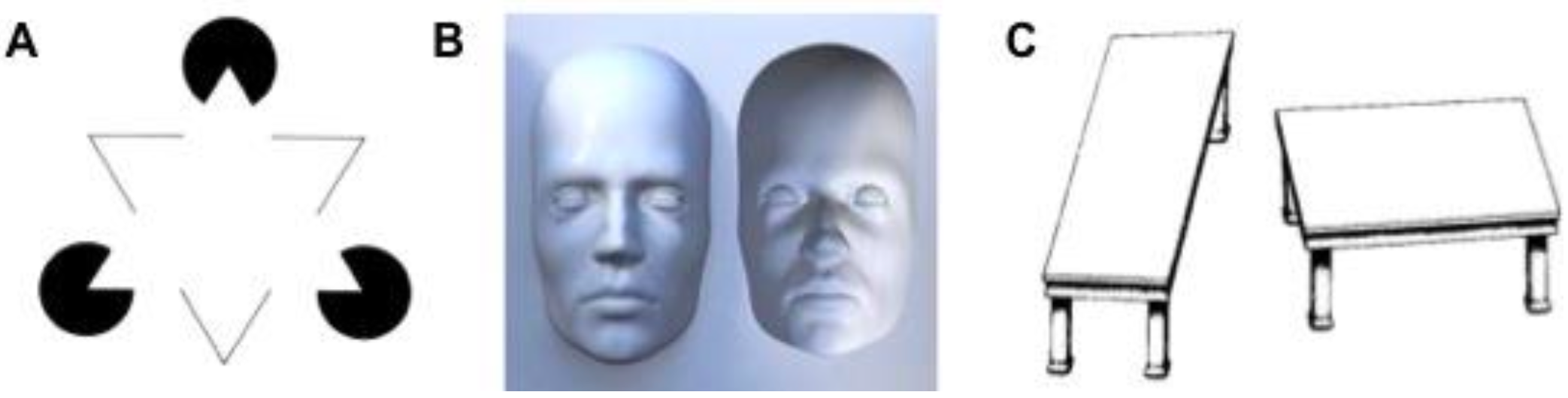
Figure 1: (?) A. The Kanizsa triangle illusion: It looks as if a white triangle overlays the other objects. B. The hollow-face illusion: A strong bias towards the natural convex face (left) suppresses the perception of the concave mask (right) even with the atypical light source from the bottom. C. Shepard’s table illusion: The two-dimensional images of the tabletop parallelograms are identical. A strong bias towards a 3D interpretation causes a perception of the further depth of the table on the left.

All the above discussions motivate us to ask how formal logic, as the laws of human thought, can be seen in terms of Bayesian models. The generative logic (?) uses a Bayesian method to model how data cause symbolic knowledge. Probabilistic reasoning with symbolic knowledge is modelled as a process of going the causality forwards and backwards with a linear time complexity with respect to the number of data. In a nutshell, the generative logic solves an inverse problem of the interpretation of formal logic, referred to as an inverse interpretation, as opposed to the inverse entailment (?) and inverse deduction (?). Its probabilistic reasoning is equivalent to the maximum likelihood estimation and is a refinement of the classical consequence relation with maximal consistent sets, which evidence statistical and logical correctness, respectively.

The generative logic especially tackles the following three fundamental assumptions of the existing prominent approaches including Bayesian networks (?), the probabilistic relational model (PRM) (?), probabilistic logic programming (PLP) (?) and Markov logic networks (MLN) (?). First, the generative logic needs no conditional independence assumption, which imposes each random variable of probabilistic systems to depend only on a small number of other random variables for computational tractability. Second, it needs no consistency assumption, which imposes logical systems to have consistent background knowledge, otherwise everything is derived due to the principle of explosion. Third, it needs no disconnection assumption, which imposes probabilistic logic systems to have both statistical and logical machineries. The statistical machinery is in charge of learning probabilities of logical sentences from data whereas the logical machinery is in charge of reasoning with the learnt logical sentences.

However, the generative logic still lacks a full logical characterisation. The above-mentioned relation to maximal consistent sets holds under the assumption that no model of formal logic has a probability of zero. The assumption can be ideal but too strict in practice as it implies that every state of the world can occur. The assumption needs to be removed to see the theoretical limits of the generative logic. Moreover, no justification is given for the extensibility of the generative logic. As evidenced by hidden Markov models and Kalman filters, Bayesian networks are extensible for temporal reasoning. The theory needs to be discussed in light of a real-world problem to see the practical prospect of the combination of Bayesian models and formal logic.

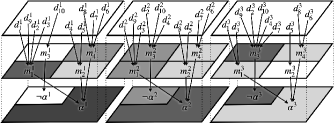
Figure 2: A schematic diagram of the generative model for temporal symbolic reasoning. Each top layer is a probability distribution over data, each middle layer is over models of formal logic, and each bottom layer is over symbolic knowledge. A darker colour indicates a higher probability. A lower layer is an abstraction (i.e., selective ignorance) of the upper layer. Time runs discretely from the left hierarchy to the right.

In this paper, we give a simple theory of inference to reason logically fully from data over time, and then fully characterise the theory in terms of a logical consequence relation introduced in this paper. Let $d_{k}^{t}$, $m_{n}^{t}$ and $\alpha^{t}$ be the $k$th data at time $t$, $n$th model at time $t$ and the truth value of the logical sentence $\alpha$ at time $t$, respectively. We will formalise the following probabilistic process of how dynamic data causes symbolic knowledge via temporal models.

$$p(\alpha^{t})= \sum_{n}p(\alpha^{t}|m_{n}^{t})p(m_{n}^{t})$$

$$= \sum_{n}p(\alpha^{t}|m_{n}^{t})\sum_{k}p(m_{n}^{t}|d_{k}^{t})p(d_{k}^{t}),$$

Figure 2 illustrates how to see the calculation as a generative process causing symbolic knowledge (on the bottom) from dynamic data (on the top layer). Let $\Delta^{t}$ be the set of truth values of logical sentences. We will look at the fact that the conditional probability, given as $p(\alpha^{t}|\Delta^{t})=\sum_{n}p(\alpha^{t}|m_{n}^{t})p(m_{n}^{t}|\Delta^{t})$, refines logical consequence relations. Here, $p(\alpha^{t}|m_{n}^{t})$ intuitively represents the probability that $\alpha$ is true in $m_{n}$ at time $t$, i.e., an interpretation, and $p(m_{n}^{t}|\Delta^{t})$ the probability that the model making all the sentences in $\Delta$ true is $m$ at time $t$, i.e., an inverse interpretation. We theoretically analyse the logical and statistical correctness of the probabilistic reasoning.

This paper contributes to interdisciplinary fields. In formal logic, the two major approaches to logical consequence relations are model checking and theorem proving (?). The Bayesian model introduced in this paper falls into another category that can be referred to as data checking. The time complexity of data checking is linear with respect to the number of data (see Equation 1). This is in contrast to the time complexity of model checking, which is exponential with respect to the number of symbols in propositional logic and is unbounded in predicate logic. The improvement comes as a result of the fact that data checking ignores all the models without data. Data checking is thus intrinsically a better approach to a consequence relation for commonsense reasoning (see Section 4). In AI, most of the modern systems across logic and probability theory (e.g., (?; ?; ?; ?)) treat learning and reasoning separately. The Bayesian model introduced in this paper unifies statistical learning from dynamic data and a sort of logical reasoning from temporal models. Probabilistic reasoning with the Bayesian model corresponds to a sort of logical reasoning with uncertain knowledge (see Corollary 1) obtained by the maximum likelihood estimation (see Equations 2, 3 and 4). Finally, we provide the neuroscience community with a new fully data-driven Bayesian model (see Theorems 1, 2, 3 and 4). As discussed above, the exact posterior distribution can be calculated using the Bayesian model with a linear time complexity. This fact challenges the motivation behind the use of approximate Bayesian methods in neuroscience, e.g., the Markov chain Monte Carlo method (?) and the variational Bayesian method (?). Neuroscience validation, however, is beyond the scope of this paper.

In the next section, we discuss a Bayesian model for temporal logical reasoning. In Section 3, we look at the statistical and logical correctness of the model and then define several inference patterns for temporal inference tasks. In Section 4, we apply the inference patterns to discuss a localisation problem. Section 5 summarises the results.

2 Generative Logic with Time

2.1 Temporal Probabilistic Models

Let ${\cal D}=\{\bm{d}_{1},\bm{d}_{1},...,\bm{d}_{K}\}$ be a finite multiset of sequences of data, where $\bm{d}_{k}=(d_{k}^{1},d_{k}^{2},...,d_{k}^{T})$ is a finite sequence of data and $d_{k}^{t}$ is the $k$th data at time $t$, for all $k$ and $t$ such that $1\leq k\leq K$ and $1\leq t\leq T$. $D$ is a random variable of data whose realisations are elements of ${\cal D}$. For all $\bm{d}_{k}\in{\cal D}$, we define the probability of $\bm{d}_{k}$ as $p(D=\bm{d}_{k})=\frac{1}{K}$. The probability distribution over $K$ sequential data is thus a uniform distribution.

The formal language we assume in this paper is a propositional language denoted by ${\cal L}$. ${\cal M}=\{m_{1},m_{2},...,m_{N}\}$ is a set of models of ${\cal L}$. ${\cal D}$ is assumed to be complete with respect to ${\cal M}$. It means that each data in $\bm{d}_{k}$ is an instance of a single model in ${\cal M}$, for all $k$ such that $1\leq k\leq K$. We use function $m$ that maps $\bm{d}_{k}$ to the sequence of such single models. $m(\bm{d}_{k})^{t}$ refers to the $t$th element of $m(\bm{d}_{k})$. $M^{t}$ is a random variable of models at time $t$ whose realisations are elements of ${\cal M}$, for all $t$ such that $1\leq t\leq T$. For all models $m_{n}\in{\cal M}$ at any time $t$ and data $\bm{d}_{k}\in{\cal D}$, we define the conditional probability of $m_{n}$ given $\bm{d}_{k}$ as follows.

$$p(M^{t}=m_{n}|D=\bm{d}_{k})=\begin{cases}1&\text{if }m_{n}=m(\bm{d}_{k})^{t}\\ 0&\text{otherwise }\end{cases}$$

Thus, the probability of model $m_{n}$ at time $t$ given data $\bm{d}_{k}$ is one if and only if the $k$th data at time $t$, i.e., $d_{k}^{t}\in\bm{d}_{k}$, is an instance of the model $m_{n}$.

Next, we give a probabilistic representation of the interpretation of formal logic. Ordinary formal logics consider an interpretation on each model. The interpretation is a function that maps each formula to a truth value, which represents knowledge of the world. The truth value of a logical formula depends on time. For any formula $\alpha\in{\cal L}$, $\alpha^{t}$ is a random variable of $\alpha$ at time $t$ whose realisations are 0 and 1, denoting false and true, respectively. We introduce variable $\mu\in[0,1]$ to denote the extent to which each model influences the interpretation. Concretely, $\mu$ denotes the probability that a formula is interpreted as being true (resp. false) in a model where it is true (resp. false). $1-\mu$ is therefore the probability that a formula is interpreted as being true (resp. false) in a model where it is false (resp. true). We assume that each formula is a random variable whose realisations are 0 and 1, denoting false and true, respectively. For all models $m_{n}\in{\cal M}$ and formulae $\alpha^{t}$, we define the conditional probability of each truth value of $\alpha^{t}$ given $m_{n}$, as follows.

$$p(\alpha^{t}=1|M^{t}=m_{n})=\begin{cases}\mu&\text{if }m_{n}\in\llbracket\alpha^{t}=1\rrbracket\\ 1-\mu&\text{otherwise }\end{cases}$$

$$p(\alpha^{t}=0|M^{t}=m_{n})=\begin{cases}\mu&\text{if }m_{n}\in\llbracket\alpha^{t}=0\rrbracket\\ 1-\mu&\text{otherwise }\end{cases}$$

Here, $\llbracket\alpha^{t}=1\rrbracket$ denotes the set of all models in which $\alpha$ is true, and $\llbracket\alpha^{t}=0\rrbracket$ the set of all models in which $\alpha$ is false. The above expressions can be simply written as a Bernoulli distribution with parameter $\mu\in[0,1]$, i.e.,

$$p(\alpha^{t}|M^{t}=m_{n})=\mu^{\llbracket\alpha^{t}\rrbracket_{m_{n}}}(1-\mu)^{1-\llbracket\alpha^{t}\rrbracket_{m_{n}}}.$$

Here, $\llbracket\alpha^{t}\rrbracket_{m_{n}}$ is a function such that $\llbracket\alpha^{t}\rrbracket_{m_{n}}=1$ if $m_{n}\in\llbracket\alpha^{t}\rrbracket$ and $\llbracket\alpha^{t}\rrbracket_{m_{n}}=0$ otherwise. Recall that $\alpha^{t}$ is a random variable, and so $\llbracket\alpha^{t}\rrbracket_{m_{n}}$ is either $\llbracket\alpha^{t}=0\rrbracket_{m_{n}}$ or $\llbracket\alpha^{t}=1\rrbracket_{m_{n}}$.

In ordinary formal logics, the truth value of each formula is independently determined given a model. In probability theory, this means that the truth values of any two formulae $\alpha_{1}^{t}$ and $\alpha_{2}^{t}$ are conditionally independent given a model $m_{n}$, i.e., $p(\alpha_{1}^{t},\alpha_{2}^{t}|M^{t}=m_{n})=p(\alpha_{1}^{t}|M^{t}=m_{n})p(\alpha_{2}^{t}|M^{t}=m_{n})$, for all $t$. Note that the conditional independence holds not only for atomic formulae but for compound formulae. However, the independence $p(\alpha_{1}^{t},\alpha_{2}^{t})=p(\alpha_{1}^{t})p(\alpha_{2}^{t})$ generally holds neither for atomic nor compound formulae. Let $\Gamma$ be a multiset $\{\alpha_{1},\alpha_{2},...,\alpha_{J}\}$ of formulae in ${\cal L}$. We use symbol $\Gamma^{t}$ to represent the multiset $\{\alpha_{1}^{t},\alpha_{2}^{t},...,\alpha_{J}^{t}\}$ of the random variables at time $t$. The probability of $\Gamma^{t}$ is given as follows.

$$p(\Gamma^{t}|M^{t}=m_{n})=\prod_{j=1}^{J}p(\alpha_{j}^{t}|M^{t}=m_{n})$$

Figure 3 shows the graphical model of the generative logic we defined in this section. It shows that sequential data is sliced by time and then fed into the corresponding models. For the sake of simplicity, we use symbols $\bm{X}^{1:t}$ to denote the set $\{X^{1},X^{2},...,X^{t}\}$ of random variables $X^{t}$, and we omit $1:t$ if $t=T$. Given a value of the parameter $\mu$, they provide the full joint distribution over all the random variables, i.e., $p(\bm{\Gamma},\bm{M},D)$. In this paper, we refer to $\{p(\bm{\Gamma}|\bm{M},\mu)$, $p(\bm{M}|D)$, $p(D)\}$ as a generative logic.

Proposition 1.

$p(\alpha^{t}=0)=p(\neg\alpha^{t}=1)$ holds, for all $t$ and $\alpha\in{\cal L}$.

Proof.

From the definition, we have

$$p(\neg\alpha^{t}=1)=\sum_{n}p(\neg\alpha^{t}=1|M^{t}=m_{n})p(M^{t}=m_{n})$$

$$= \sum_{n}\mu^{[\![\neg\alpha^{t}=1]\!]_{M^{t}=m_{n}}}(1-\mu)^{1-[\![\neg\alpha^{t}=1]\!]_{M^{t}=m_{n}}}p(M^{t}=m_{n})$$

$$= \sum_{n}\mu^{[\![\alpha^{t}=0]\!]_{M^{t}=m_{n}}}(1-\mu)^{1-[\![\alpha^{t}=0]\!]_{M^{t}=m_{n}}}p(M^{t}=m_{n})$$

$$= \sum_{n}p(\alpha^{t}=0|M^{t}=m_{n})p(M^{t}=m_{n})=p(\alpha^{t}=0).$$

This proof holds regardless of the value of $\mu$. ∎

In what follows, we therefore replace $\alpha^{t}=0$ by $\lnot\alpha^{t}=1$ and then abbreviate $\lnot\alpha^{t}=1$ to $\lnot\alpha^{t}$. We also abbreviate $M^{t}=m_{n}$ to $m_{n}$ and $D=\bm{d}_{k}$ to $\bm{d}_{k}$ for simplicity.

Figure 3: The generative logic is about a formal representation of problem-independent logical interpretation and its inversion. It is not about a formal representation of problem-dependent uncertain domain knowledge.

Example 1.

Let $\{p(\bm{\Gamma}|\bm{M},\mu=1),p(\bm{M}|D),p(D)\}$ be a generative logic built on ${\cal D}=\{d_{k}^{t}|1\leq k\leq 5,1\leq t\leq 3\}$. Suppose that $d_{k}^{t}$ is data about weather $r$ (meaning ‘rain’) and ground condition $w$ (meaning ‘wet’) collected on day $t$ by person $k$. Suppose $m(\bm{d}_{1})=(m_{1},m_{1},m_{2})$, $m(\bm{d}_{2})=(m_{2},m_{4},m_{3})$, $m(\bm{d}_{3})=(m_{1},m_{4},m_{4})$, $m(\bm{d}_{4})=(m_{1},m_{2},m_{4})$ and $m(\bm{d}_{5})=(m_{3},m_{2},m_{2})$ where $m_{1}$ satisfies neither $r$ nor $w$, $m_{2}$ satisfies only $w$, $m_{3}$ satisfies only $r$, and $m_{4}$ satisfies both $r$ and $w$.

$$p(w^{3}|r^{3})= \frac{\sum_{n=1}^{4}\sum_{k=1}^{5}p(w^{3}|m_{n})p(r^{3}|m_{n})p(m_{n}|\bm{d}_{k})}{\sum_{n=1}^{4}\sum_{k=1}^{5}p(r^{3}|m_{n})p(m_{n}|\bm{d}_{k})}$$

$$= \frac{\sum_{k=1}^{5}p(w^{3}|m(\bm{d}_{k})^{3})p(r^{3}|m(\bm{d}_{k})^{3})}{\sum_{k=1}^{5}p(r^{3}|m(\bm{d}_{k})^{3})}$$

$$= \frac{\sum_{k=1}^{5}\llbracket w^{3}\rrbracket_{m(\bm{d}_{k})^{3}}\llbracket r^{3}\rrbracket_{m(\bm{d}_{k})^{3}}}{\sum_{k=1}^{5}\llbracket r^{3}\rrbracket_{m(\bm{d}_{k})^{3}}}=\frac{2}{3}$$

In line 1, we brought all the random variables and then cancelled $p(\bm{d}_{k})=1/5$, for all $k$. In line 2, we used $\sum_{n}p(\alpha^{t}|m_{n})p(m_{n}|\bm{d}_{k})=p(\alpha^{t}|m(\bm{d}_{k})^{t})$, for all $\alpha$ and $t$.

As demonstrated in Example 1, the summation over models can be eliminated by the assumption that data are complete with respect to the models. In general, we have

$$p(\alpha^{t})=\sum_{k=1}^{K}p(\bm{d}_{k})\sum_{n=1}^{N}p(\alpha^{t}|m_{n})p(m_{n}|\bm{d}_{k})$$ (1)

$$=\sum_{k=1}^{K}\frac{1}{K}\sum_{n=1}^{N}[\![\alpha^{t}]\!]_{m(\bm{d}_{k})^{t}}p(m_{n}|\bm{d}_{k})=\frac{1}{K}\sum_{k=1}^{K}[\![\alpha]\!]_{m(\bm{d}_{k})^{t}}.$$

The number of models increases exponentially with respect to the number of symbols in propositional logic and unbounded in predicate logic. Equation (1) thus guarantees the scalability of the generative logic.

3 Theoretical Correctness

3.1 Maximum Likelihood Estimation

Let $\{p(\bm{\Gamma}|\bm{M},\mu),p(\bm{M}|D),p(D)\}$ be a temporal generative logic. We look at the statistical properties of the probability distribution over models over time. Let $m_{n}^{t}$ and $m_{o}^{u}$ be the $n$th model at time $t$ and $o$th model at time $u$, respectively. Their joint probability given by the temporal generative logic can be written as

$$p(m_{n}^{t},m_{o}^{u})= \sum_{\bm{d}}p(m_{n}^{t}|\bm{d})p(m_{o}^{u}|\bm{d})p(\bm{d})$$

$$= \frac{1}{K}\sum_{\bm{d}}p(m_{n}^{t}|\bm{d})p(m_{o}^{u}|\bm{d})=\frac{K_{n,o}}{K},$$ (2)

where $K$ is the total number of data and $K_{n,o}$ is the number of data in the model $m_{n}$ at time $t$ and in the model $m_{o}$ at time $u$ (see Table 1).

Now, we ask how the joint distribution $p(M^{t},M^{u})$ can be characterised in terms of maximum likelihood estimation, which is the most often used method to estimate a probability distribution only from data. As illustrated in Table 1, the joint distribution can be seen as a categorical distribution with parameter $\Phi=(\phi_{1,1},\phi_{1,2},...,\phi_{N,N})$. Assuming that each data is independent and identically distributed, the parameter $\Phi$ maximising the likelihood of data, denoted by $\Phi_{ML}$, can be written as follows.

$$\Phi_{ML}= \operatorname*{arg\,max}_{\Phi}p({\cal D}|\Phi)=\operatorname*{arg\,max}_{\Phi}\phi_{1,1}^{K_{1,1}}\phi_{1,2}^{K_{1,2}}...$$

$$...\phi_{N,N-1}^{K_{N,N-1}}(1-\phi_{1,1}-\phi_{1,2}-...-\phi_{N,N-1})^{K_{N,N}}.$$

$\Phi$ maximises the likelihood $p({\cal D}|\Phi)$ if and only if it maximises its log-likelihood $L(\Phi)$ given as follows.

$$L(\Phi)=K_{1,1}\log\phi_{1,1}+K_{1,2}\log\phi_{1,2}+...+K_{N,N-1}$$

$$\log\phi_{N,N-1}+K_{N,N}\log(1-\phi_{1,1}-\phi_{1,2}-...-\phi_{N,N-1}).$$

$\Phi$ maximising the log-likelihood can be found by solving the simultaneous equations given as follows, for all $n$ and $o$.

$$\frac{\partial L(\Phi)}{\partial\phi_{n,o}}=\frac{K_{n,o}}{\phi_{n,o}}-\frac{K_{N,N}}{1-\phi_{1,1}-\phi_{1,2}-...-\phi_{N,N-1}}=0$$

The solution to the simultaneous equations turns out to be

$$\Phi_{ML}=\left(\frac{K_{1,1}}{K},\frac{K_{1,2}}{K},...,\frac{K_{N,N}}{K}\right).$$ (3)

We thus have $p(M^{t},M^{u})=\Phi_{ML}$. Namely, $p(m_{n}^{t},m_{o}^{u})=K_{n,o}/K$ is the ratio of the number of data in the model $m_{n}$ at time $t$ and the model $m_{o}$ at time $u$ to the total number of data. It is observed that Equation (2) we derived using the temporal generative logic is the maximum likelihood estimate. In general, the joint distribution over models given by the temporal generative logic can be written as

$$p(m_{n}^{1},m_{o}^{2},...,m_{p}^{T})=\frac{K_{n,o,...,p}}{K},$$

where $\frac{K_{n,o,...,p}}{K}$ is the maximum likelihood estimate, and thus $K_{n,o,...,p}$ is the number of data in $m_{n}$ at time $1$, $m_{o}$ at time $2$, $m_{p}$ at time $T$, and so on.

Table 1: $\Phi=\left(\phi_{n,o}|1\leq n,o\leq N\right)$ is the joint probability distribution over the models with time $t$ and $u$, i.e., $p(M^{t},M^{u})$. $K_{n,o}$ is the number of data such that it is in the model $m_{n}$ at time $t$ and in the model $m_{o}$ at time $u$. $K_{n}=\sum_{o}K_{n,o}$ is the number of data in $m_{n}$ at $t$, and $K=\sum_{n,o}K_{n,o}$ is the total number of data.

	$m_{1}^{u}$		$m_{o}^{u}$		$m_{N}^{u}$
$m_{1}^{t}$	$\phi_{1,1}(K_{1,1})$		$\phi_{1,o}(K_{1,o})$		$\phi_{1,N}(K_{1,N})$
			…
$m_{n}^{t}$	$\phi_{n,1}(K_{n,1})$	…	$\phi_{n,o}(K_{n,o})$	…	$\phi_{n,N}(K_{n,N})$
			…
$m_{N}^{t}$	$\phi_{N,1}(K_{N,1})$		$\phi_{N,o}(K_{N,o})$		$\phi_{N,N}(K_{N,N})$

We next look at the statistical properties of the probability distribution over formulae over time. On the temporal generative logic, we have

$$p(\alpha^{t},\beta^{u})= \sum_{m_{n}^{t}}\sum_{m_{o}^{u}}p(\alpha^{t},\beta^{u}|m_{n}^{t},m_{o}^{u})p(m_{n}^{t},m_{o}^{u})$$

$$= \sum_{m_{n}^{t}}\sum_{m_{o}^{u}}p(\alpha^{t}|m_{n}^{t},m_{o}^{u})p(\beta^{u}|m_{n}^{t},m_{o}^{u})p(m_{n}^{t},m_{o}^{u})$$

$$= \sum_{m_{n}^{t}}p(\alpha^{t}|m_{n}^{t})\sum_{m_{o}^{u}}p(\beta^{u}|m_{o}^{u})p(m_{n}^{t},m_{o}^{u}).$$

The second equation holds as $\alpha^{t}$ and $\beta^{u}$ are conditionally independent given $m_{n}^{t}$ and $m_{o}^{u}$. The third equation holds as $\alpha^{t}$ (resp. $\beta^{u}$) is conditionally independent of $m_{o}^{u}$ (resp. $m_{n}^{t}$) given $m_{n}^{t}$ (resp. $m_{o}^{u}$). Given $\mu=1$ or $\mu\to 1$, we have

$$p(\alpha^{t},\beta^{u})= \sum_{m_{n}^{t}\in[\![\alpha^{t}]\!]}\sum_{m_{o}^{u}\in[\![\beta^{u}]\!]}p(m_{n}^{t},m_{o}^{u})$$

$$= \sum_{m_{n}^{t}\in[\![\alpha^{t}]\!]}\sum_{m_{o}^{u}\in[\![\beta^{u}]\!]}\frac{K_{n,o}}{K}.$$ (4)

Probability theory and propositional logic are typically combined so that it satisfies $p(\alpha)=\sum_{m_{n}\in[\![\alpha]\!]}p(m_{n})$, for all propositional sentences $\alpha$ (?). In Equation (4), the first equation guarantees a natural extension of the classical approach. The second equation shows that the probabilities of the models are equal to the maximum likelihood estimate (see Equation (3)). In general, the joint distribution over formulae given by the temporal generative logic can be written as

$$p(\alpha^{1},\beta^{2},...,\gamma^{T})=\sum_{m_{n}^{1}\in[\![\alpha^{1}]\!]}\sum_{m_{o}^{2}\in[\![\beta^{2}]\!]}...\sum_{m_{p}^{T}\in[\![\gamma^{T}]\!]}\frac{K_{n,o,...,p}}{K}.$$

This result implies $p(\alpha^{t},\beta^{t},...,\gamma^{t})$ $=\sum_{m_{n}^{t}\in[\![\alpha^{t},\beta^{t},...,\gamma^{t}]\!]}\frac{K_{n}}{K}$, which is the static case discussed in the paper (?). It is obvious from Equation (4) that a conditional probability distribution over time is given by

$$p(\beta^{u}|\alpha^{t})= \frac{p(\beta^{u},\alpha^{t})}{p(\alpha^{t})}=\frac{\sum_{m_{o}^{u}\in[\![\beta^{u}]\!]}\sum_{m_{n}^{t}\in[\![\alpha^{t}]\!]}p(m_{o}^{u},m_{n}^{t})}{\sum_{m_{n}^{t}\in[\![\alpha^{t}]\!]}p(m_{n}^{t})}$$

$$= \frac{\sum_{m_{o}^{u}\in[\![\beta^{u}]\!]}\sum_{m_{n}^{t}\in[\![\alpha^{t}]\!]}K_{n,o}}{\sum_{m_{n}^{t}\in[\![\alpha^{t}]\!]}K_{n}}.$$

3.2 Empirical Consequence Relation

Let $\{p(\bm{\Gamma}|\bm{M},\mu),p(\bm{M|D}),p(D)\}$ be a generative logic. From the above-mentioned assumption that each data is complete with respect to models, we have

$$p(\bm{\Gamma})= \sum_{\bm{d}}\sum_{m}p(\bm{\Gamma}|m,\mu)p(m|\bm{d})p(\bm{d})$$

$$= \sum_{\bm{d}}p(\bm{\Gamma}|m(\bm{d}),\mu)p(\bm{d}).$$

Consider $\{p^{\prime}(\bm{\Gamma}|D,\mu)$, $p(D)\}$ where $p^{\prime}(\bm{\Gamma}|D,\mu)$ is defined as $p(\bm{\Gamma}|m(D),\mu)$. Given a value of $\mu$, it gives the joint distribution $p(\bm{\Gamma},D)$. It is thus another generative logic excluding the random variables of models. We have now

$$p^{\prime}(\bm{\Gamma})=\sum_{\bm{d}}p^{\prime}(\bm{\Gamma}|\bm{d},\mu)p(\bm{d})=\sum_{\bm{d}}p(\bm{\Gamma}|m(\bm{d}),\mu)p(\bm{d}).$$

The above result shows that $\{p(\bm{\Gamma}|\bm{M},\mu),p(\bm{M|D}),p(D)\}$ is equivalent to $\{p^{\prime}(\bm{\Gamma}|D,\mu)$, $p(D)\}$ in terms of the probability distribution over a set of formulae. In this section, we write the latter generative logic simply as $\{p(\bm{\Gamma}|D,\mu)$, $p(D)\}$ and use it without distinction. We also omit time $t$ if it is obvious from the context.

Definition 1 (Evidence).

Let $\bm{d}\in{\cal D}$ and $\Delta\subseteq{\cal L}$. $\bm{d}$ is an evidence of $\Delta$ if $\alpha$ is true in $m(\bm{d})$, for all $\alpha\in\Delta$.

In this paper, we assume that any subset of the multiset ${\cal D}$ is also a multiset. For $\Delta\in{\cal L}$, we use symbol $\langle\!\langle\Delta\rangle\!\rangle$ to denote the set of the evidences of $\Delta$, i.e., $\langle\!\langle\Delta\rangle\!\rangle=\{\bm{d}\in{\cal D}|\bm{d}$ is an evidence of $\Delta\}$. We refer to $\Delta$ as founded if $\langle\!\langle\Delta\rangle\!\rangle\neq\emptyset$ and unfounded otherwise.

Definition 2 (Maximal founded sets).

Let $\Delta\subseteq{\cal L}$. $S\subseteq\Delta$ is a maximal founded subset of $\Delta$ if $\langle\!\langle S\rangle\!\rangle\neq\emptyset$ and $\langle\!\langle S\cup\{\alpha\}\rangle\!\rangle=\emptyset$, for all $\alpha\in\Delta\setminus S$.

We use the symbol $MFS(\Delta)$ to denote the set of the cardinality-maximal founded subsets of $\Delta$ and the symbol $|X|$ to denote the number of elements in a set $X$. We use symbol $\langle\!\langle\Delta\rangle\!\rangle^{\prime}$ to denote the set of the evidences of the cardinality-maximal founded subsets of $\Delta$, i.e., $\langle\!\langle\Delta\rangle\!\rangle^{\prime}=\bigcup_{S\in MFS(\Delta)}\langle\!\langle S\rangle\!\rangle$. Obviously, $\langle\!\langle\Delta\rangle\!\rangle=\langle\!\langle\Delta\rangle\!\rangle^{\prime}$ if $\langle\!\langle\Delta\rangle\!\rangle\neq\emptyset$. The following theorem relates the conditional probability distribution to the evidence of the formulae.

Theorem 1.

Let $\{p(\bm{\Gamma}|D,\mu),p(D)\}$ be a generative logic such that $\mu\to 1$. For all $\Omega,\Delta\subseteq{\cal L}$ such that $\langle\!\langle\Delta\rangle\!\rangle^{\prime}\neq\emptyset$,

$$p(\Omega|\Delta)=\frac{|\langle\!\langle\Omega\rangle\!\rangle\cap\langle\!\langle\Delta\rangle\!\rangle^{\prime}|}{|\langle\!\langle\Delta\rangle\!\rangle^{\prime}|}.$$

Proof.

We use symbol $|X|_{m(\bm{d})}$ to denote the number of formulae in $X$ that are true in $m(\bm{d})$, i.e. $|X|_{m(\bm{d})}=\sum_{\beta^{t}\in X}[\![\beta^{t}]\!]_{m(\bm{d})^{t}}$. Dividing data in $\langle\!\langle\Delta\rangle\!\rangle^{\prime}$ and the others, we have

$$p(\Omega|\Delta)=\lim_{\mu\to 1}\frac{\sum_{\bm{d}}p(\Omega|\bm{d},\mu)p(\Delta|\bm{d},\mu)}{\sum_{\bm{d}}p(\Delta|\bm{d},\mu)}=\lim_{\mu\to 1}$$

$$\frac{\displaystyle{\sum_{\hat{\bm{d}}\in\langle\!\langle\Delta\rangle\!\rangle^{\prime}}p(\Omega|\hat{\bm{d}},\mu)p(\Delta|\hat{\bm{d}},\mu)+\sum_{\bm{d}\notin\langle\!\langle\Delta\rangle\!\rangle^{\prime}}p(\Omega|\bm{d},\mu)p(\Delta|\bm{d},\mu)}}{\displaystyle{\sum_{\hat{\bm{d}}\in\langle\!\langle\Delta\rangle\!\rangle^{\prime}}p(\Delta|\hat{\bm{d}},\mu)+\sum_{\bm{d}\notin\langle\!\langle\Delta\rangle\!\rangle^{\prime}}p(\Delta|\bm{d},\mu)}}.$$

Now, $p(X|m)$ can be developed as follows, for all $\bm{d}$.

$$p(X|\bm{d})= \prod_{\beta\in X}p(\beta|\bm{d})=\prod_{\beta\in X}\mu^{[\![\beta]\!]_{m(\bm{d})}}(1-\mu)^{1-[\![\beta]\!]_{m(\bm{d})}}$$

$$= \mu^{\sum_{\beta\in X}[\![\beta]\!]_{m(\bm{d})}}(1-\mu)^{\sum_{\beta\in X}(1-[\![\beta]\!]_{m(\bm{d})})}$$

$$= \mu^{|X|_{m(\bm{d})}}(1-\mu)^{|X|-|X|_{m(\bm{d})}}$$

We have $p(\Omega|\Delta)=\lim_{\mu\rightarrow 1}\frac{\sum_{\hat{\bm{d}}\in\langle\!\langle\Delta\rangle\!\rangle^{\prime}}W+\sum_{\bm{d}\notin\langle\!\langle\Delta\rangle\!\rangle^{\prime}}X}{\sum_{\hat{\bm{d}}\in\langle\!\langle\Delta\rangle\!\rangle^{\prime}}Y+\sum_{\bm{d}\notin\langle\!\langle\Delta\rangle\!\rangle^{\prime}}Z}$ where

$$W=\textstyle{\mu^{|\Omega|_{m(\hat{\bm{d}})}}(1-\mu)^{|\Omega|-|\Omega|_{m(\hat{\bm{d}})}}\mu^{|\Delta|_{m(\hat{\bm{d}})}}(1-\mu)^{|\Delta|-|\Delta|_{m(\hat{\bm{d}})}}}$$

$$X=\textstyle{\mu^{|\Omega|_{m(\bm{d})}}(1-\mu)^{|\Omega|-|\Omega|_{m(\bm{d})}}\mu^{|\Delta|_{m(\bm{d})}}(1-\mu)^{|\Delta|-|\Delta|_{m(\bm{d})}}}$$

$$Y=\textstyle{\mu^{|\Delta|_{m(\hat{\bm{d}})}}(1-\mu)^{|\Delta|-|\Delta|_{m(\hat{\bm{d}})}}}$$

$$Z=\textstyle{\mu^{|\Delta|_{m(\bm{d})}}(1-\mu)^{|\Delta|-|\Delta|_{m(\bm{d})}}}.$$

Now, if $\bm{d}\notin\langle\!\langle\Delta\rangle\!\rangle^{\prime}$ then $\bm{d}$ is an evidence of a subset of $\Delta$ that is not a cardinality-maximal founded subset of $\Delta$. Therefore, there is $\hat{\bm{d}}\in\langle\!\langle\Delta\rangle\!\rangle^{\prime}$ such that $|\Delta|_{m(\bm{d})}<|\Delta|_{m(\hat{\bm{d}})}$. $|\Delta|_{m(\hat{\bm{d}_{1}})}=|\Delta|_{m(\hat{\bm{d}_{2}})}$ by definition, for all $\hat{\bm{d}_{1}},\hat{\bm{d}_{2}}\in\langle\!\langle\Delta\rangle\!\rangle^{\prime}$. The fraction thus can be simplified by dividing the denominator and numerator by $(1-\mu)^{|\Delta|-|\Delta|_{m(\hat{\bm{d}})}}$. We thus have $p(\Omega|\Delta)=\lim_{\mu\rightarrow 1}\frac{\sum_{\hat{\bm{d}}\in\langle\!\langle\Delta\rangle\!\rangle^{\prime}}W^{\prime}+\sum_{\bm{d}\notin\langle\!\langle\Delta\rangle\!\rangle^{\prime}}X^{\prime}}{\sum_{\hat{\bm{d}}\in\langle\!\langle\Delta\rangle\!\rangle^{\prime}}Y^{\prime}+\sum_{\bm{d}\notin\langle\!\langle\Delta\rangle\!\rangle^{\prime}}Z^{\prime}}$ where

$$W^{\prime}=\textstyle{\mu^{|\Omega|_{m(\hat{\bm{d}})}}(1-\mu)^{|\Omega|-|\Omega|_{m(\hat{\bm{d}})}}\mu^{|\Delta|_{m(\hat{\bm{d}})}}}$$

$$X^{\prime}=\textstyle{\mu^{|\Omega|_{m(\bm{d})}}(1-\mu)^{|\Omega|-|\Omega|_{m(\bm{d})}}\mu^{|\Delta|_{m(\bm{d})}}(1-\mu)^{|\Delta|_{m(\hat{\bm{d}})}-|\Delta|_{m(\bm{d})}}}$$

$$Y^{\prime}=\textstyle{\mu^{|\Delta|_{m(\hat{\bm{d}})}}}$$

$$Z^{\prime}=\textstyle{\mu^{|\Delta|_{m(\bm{d})}}(1-\mu)^{|\Delta|_{m(\hat{\bm{d}})}-|\Delta|_{m(\bm{d})}}}.$$

Applying the limit operation, we can cancel out $X^{\prime}$ and $Z^{\prime}$ and have

$$p(\Omega|\Delta)= \frac{\sum_{\hat{\bm{d}}\in\langle\!\langle\Delta\rangle\!\rangle^{\prime}}1^{|\Omega|_{m(\hat{\bm{d}})}}0^{|\Omega|-|\Omega|_{m(\hat{\bm{d}})}}1^{|\Delta|_{m(\hat{\bm{d}})}}}{\sum_{\hat{\bm{d}}\in\langle\!\langle\Delta\rangle\!\rangle^{\prime}}1^{|\Delta|_{m(\hat{\bm{d}})}}}$$

$$= \frac{\sum_{\hat{\bm{d}}\in\langle\!\langle\Delta\rangle\!\rangle^{\prime}}0^{|\Omega|-|\Omega|_{m(\hat{\bm{d}})}}}{\sum_{\hat{\bm{d}}\in\langle\!\langle\Delta\rangle\!\rangle^{\prime}}1}=\frac{|\langle\!\langle\Omega\rangle\!\rangle\cap\langle\!\langle\Delta\rangle\!\rangle^{\prime}|}{|\langle\!\langle\Delta\rangle\!\rangle^{\prime}|}.$$ (5)

In line 2, we used the fact that $0^{|\Omega|-|\Omega|_{m(\hat{\bm{d}})}}=1$ iff $|\Omega|=|\Omega|_{m(\hat{\bm{d}})}$, and $0^{|\Omega|-|\Omega|_{m(\hat{\bm{d}})}}=0$ iff $|\Omega|>|\Omega|_{m(\hat{\bm{d}})}$. ∎

To logically characterise the conditional probability, we define another consequence relation based on data.

Definition 3 (Empirical consequence).

Let $\Delta,\Omega\subseteq{\cal L}$. $\Omega$ is an empirical consequence of $\Delta$, denoted by $\Delta\mathrel{\scalebox{1.0}[1.5]{$\shortmid$}\mkern-3.1mu\raisebox{0.43057pt}{$\eqcirc$}}\Omega$, if $\langle\!\langle\Delta\rangle\!\rangle\subseteq\langle\!\langle\Omega\rangle\!\rangle$.

The following corollary shows that the empirical consequence relation with maximal founded sets characterises probabilistic reasoning on the generative logic.

Corollary 1.

Let $\{p(\bm{\Gamma}|D,\mu),p(D)\}$ be a generative logic such that $\mu\to 1$. For all $\Omega,\Delta\subseteq{\cal L}$ such that $\langle\!\langle\Delta\rangle\!\rangle^{\prime}\neq\emptyset$, $p(\Omega|\Delta)=1$ iff $S\mathrel{\scalebox{1.0}[1.5]{$\shortmid$}\mkern-3.1mu\raisebox{0.43057pt}{$\eqcirc$}}\Omega$, for all maximal founded subsets $S$ of $\Delta$.

Proof.

From Equation (5), $p(\Omega|\Delta)=1$ iff $\langle\!\langle\Delta\rangle\!\rangle^{\prime}\subseteq\langle\!\langle\Omega\rangle\!\rangle$. Since $\langle\!\langle\Delta\rangle\!\rangle^{\prime}=\bigcup_{S\in MFS(\Delta)}\langle\!\langle S\rangle\!\rangle$, $p(\Omega|\Delta)=1$ iff $\bigcup_{S\in MFS(\Delta)}\langle\!\langle S\rangle\!\rangle\subseteq\langle\!\langle\Omega\rangle\!\rangle$. ∎

The following theorem shows that probabilistic reasoning on the generative logic is reasonable even when there is no evidence of any formula in the condition.

Theorem 2.

Let $\{p(\bm{\Gamma}|D,\mu),p(D)\}$ be a generative logic such that $\mu\to 1$. For all $\Omega,\Delta\subseteq{\cal L}$ such that $\langle\!\langle\Delta\rangle\!\rangle^{\prime}=\emptyset$, $p(\Omega|\Delta)=p(\Omega)$.

Proof.

Since $\langle\!\langle\Delta\rangle\!\rangle^{\prime}=\emptyset$, we have

$$p(\Omega|\Delta)=\lim_{\mu\to 1}\frac{\sum_{\bm{d}\notin\langle\!\langle\Delta\rangle\!\rangle^{\prime}}p(\Omega|\bm{d},\mu)p(\Delta|\bm{d},\mu)p(\bm{d})}{\sum_{\bm{d}\notin\langle\!\langle\Delta\rangle\!\rangle^{\prime}}p(\Delta|\bm{d},\mu)p(\bm{d})}$$

Now, $\langle\!\langle\Delta\rangle\!\rangle^{\prime}=\bigcup_{S\in MFS(\Delta)}\langle\!\langle S\rangle\!\rangle=\emptyset$ iff no data is an evidence of any singleton of $\Delta$. We thus have

$$p(\Delta|\bm{d},\mu)=\prod_{\beta^{t}\in\Delta}p(\beta^{t}|\bm{d},\mu)=\prod_{\beta^{t}\in\Delta}\mu^{[\![\beta^{t}]\!]_{m(\bm{d})^{t}}}(1-\mu)^{1-[\![\beta^{t}]\!]_{m(\bm{d})^{t}}}$$

$$=\mu^{\sum_{\beta^{t}\in\Delta}[\![\beta^{t}]\!]_{m(\bm{d})^{t}}}(1-\mu)^{\sum_{\beta^{t}\in\Delta}(1-[\![\beta^{t}]\!]_{m(\bm{d})^{t}})}=\mu^{0}(1-\mu)^{|\Delta|}.$$

Therefore, we have

$$p(\Omega|\Delta)=\lim_{\mu\to 1}\frac{\sum_{\bm{d}\notin\langle\!\langle\Delta\rangle\!\rangle^{\prime}}p(\Omega|\bm{d},\mu)\mu^{0}(1-\mu)^{|\Delta|}p(\bm{d})}{\sum_{\bm{d}\notin\langle\!\langle\Delta\rangle\!\rangle^{\prime}}\mu^{0}(1-\mu)^{|\Delta|}p(\bm{d})}$$

$$=\lim_{\mu\to 1}\frac{\sum_{\bm{d}\notin\langle\!\langle\Delta\rangle\!\rangle^{\prime}}p(\Omega|\bm{d},\mu)p(\bm{d})}{\sum_{\bm{d}\notin\langle\!\langle\Delta\rangle\!\rangle^{\prime}}p(\bm{d})}=\lim_{\mu\to 1}\frac{\sum_{\bm{d}}p(\Omega|\bm{d},\mu)p(\bm{d})}{\sum_{\bm{d}}p(\bm{d})}$$

$$=\lim_{\mu\to 1}\sum_{\bm{d}}p(\Omega|\bm{d},\mu)p(\bm{d})=p(\Omega).$$

∎

All the above properties discussed in this section are about the relationship between formulae. The following two theorems show how the distribution over data is updated in light of the observation of formulae.

Theorem 3.

Let $\{p(\bm{\Gamma}|D,\mu),p(D)\}$ be a generative logic such that $\mu\to 1$. For all $\Delta\subseteq{\cal L}$ such that $\langle\!\langle\Delta\rangle\!\rangle^{\prime}\neq\emptyset$,

$$p(D|\Delta)=\begin{cases}\frac{1}{|\langle\!\langle\Delta\rangle\!\rangle^{\prime}|}&\text{ if }D\in\langle\!\langle\Delta\rangle\!\rangle^{\prime}\\ 0&\text{ otherwise.}\end{cases}$$

Proof.

Again, we use symbols $|\Delta|$ and $|\Delta|_{m(\bm{d})}$ to denote the number of formulae in $\Delta$ and the number of formulae in $\Delta$ that are true in $m(\bm{d})$, i.e., $|\Delta|_{m(\bm{d})}=\sum_{\beta^{t}\in\Delta}[\![\beta^{t}]\!]_{m(\bm{d})^{t}}$, respectively.

$$p(D|\Delta)= \lim_{\mu\to 1}\frac{\prod_{\beta^{t}\in\Delta}\mu^{[\![\beta^{t}]\!]_{m(D)^{t}}}(1-\mu)^{1-[\![\beta^{t}]\!]_{m(D)^{t}}}}{\sum_{\bm{d}}\prod_{\beta^{t}\in\Delta}\mu^{[\![\beta^{t}]\!]_{m(\bm{d})^{t}}}(1-\mu)^{1-[\![\beta^{t}]\!]_{m(\bm{d})^{t}}}}$$

$$= \lim_{\mu\to 1}\frac{\mu^{|\Delta|_{m(D)}}(1-\mu)^{|\Delta|-|\Delta|_{m(D)}}}{\sum_{\bm{d}}\mu^{|\Delta|_{m(\bm{d})}}(1-\mu)^{|\Delta|-|\Delta|_{m(\bm{d})}}}$$

Separating the models in $\langle\!\langle\Delta\rangle\!\rangle^{\prime}$ and the others, we have $p(D|\Delta)=\lim_{\mu\to 1}$ $\frac{X}{\sum_{\hat{\bm{d}}\in\langle\!\langle\Delta\rangle\!\rangle}Y+\sum_{\bm{d}\notin\langle\!\langle\Delta\rangle\!\rangle}Z}$ where

$$X=\mu^{|\Delta|_{m(D)}}(1-\mu)^{|\Delta|-|\Delta|_{m(D)}}$$

$$Y=\mu^{|\Delta|_{m(\hat{\bm{d}})}}(1-\mu)^{|\Delta|-|\Delta|_{m(\hat{\bm{d}})}}$$

$$Z=\mu^{|\Delta|_{m(\bm{d})}}(1-\mu)^{|\Delta|-|\Delta|_{m(\bm{d})}}.$$

Dividing the denominator and numerator by $(1-\mu)^{|\Delta|-|\Delta|_{m(\hat{\bm{d}})}}$, we have $p(D|\Delta)=\lim_{\mu\to 1}$ $\frac{X^{\prime}}{\sum_{\hat{\bm{d}}\in\langle\!\langle\Delta\rangle\!\rangle}Y^{\prime}+\sum_{\bm{d}\notin\langle\!\langle\Delta\rangle\!\rangle}Z^{\prime}}$ where

$$X^{\prime}=\mu^{|\Delta|_{m(D)}}(1-\mu)^{|\Delta|_{m(\hat{\bm{d}})}-|\Delta|_{m(D)}}$$

$$Y^{\prime}=\mu^{|\Delta|_{m(\hat{\bm{d}})}}$$

$$Z^{\prime}=\mu^{|\Delta|_{m(\bm{d})}}(1-\mu)^{|\Delta|_{m(\hat{\bm{d}})}-|\Delta|_{m(\bm{d})}}.$$

$|\Delta|_{m(\hat{\bm{d}})}>|\Delta|_{m(\bm{d})}$. Applying the limit operation, we have

$$p(D|\Delta)=\frac{1^{|\Delta|_{m(D)}}0^{|\Delta|_{m(\hat{\bm{d}})}-|\Delta|_{m(D)}}}{\sum_{\hat{\bm{d}}\in\langle\!\langle\Delta\rangle\!\rangle}1^{|\Delta|_{m(\hat{\bm{d}})}}}=\frac{0^{|\Delta|_{m(\hat{\bm{d}})}-|\Delta|_{m(D)}}}{\sum_{\hat{\bm{d}}\in\langle\!\langle\Delta\rangle\!\rangle}1}$$

$0^{|\Delta|_{m(\hat{\bm{d}})}-|\Delta|_{m(D)}}=1$ if $D\in\langle\!\langle\Delta\rangle\!\rangle^{\prime}$ and $0$ otherwise. Thus,

$$p(D|\Delta)=\begin{cases}\frac{1}{|\langle\!\langle\Delta\rangle\!\rangle^{\prime}|}&\text{ if }D\in\langle\!\langle\Delta\rangle\!\rangle^{\prime}\\ 0&\text{ otherwise.}\end{cases}$$

∎

The following theorem shows that probabilistic reasoning for data is reasonable even when there is no evidence of any formula in the condition.

Theorem 4.

Let $\{p(\bm{\Gamma}|D,\mu),p(D)\}$ be a generative logic such that $\mu\to 1$. For all $\Delta\subseteq{\cal L}$ such that $\langle\!\langle\Delta\rangle\!\rangle^{\prime}=\emptyset$, $p(D|\Delta)=p(D)$.

Proof.

Since $\langle\!\langle\Delta\rangle\!\rangle^{\prime}=\emptyset$, we have

$$p(D|\Delta)=\lim_{\mu\to 1}\frac{p(\Delta|D,\mu)p(D)}{\sum_{\bm{d}\notin\langle\!\langle\Delta\rangle\!\rangle^{\prime}}p(\Delta|\bm{d},\mu)p(\bm{d})}$$

Now, $\langle\!\langle\Delta\rangle\!\rangle^{\prime}=\bigcup_{S\in MFS(\Delta)}\langle\!\langle S\rangle\!\rangle=\emptyset$ iff no data is an evidence of any singleton of $\Delta$. For all $\bm{d}$, we thus have

$$p(\Delta|\bm{d},\mu)=\prod_{\beta^{t}\in\Delta}p(\beta^{t}|\bm{d},\mu)=\prod_{\beta^{t}\in\Delta}\mu^{[\![\beta^{t}]\!]_{m(\bm{d})^{t}}}(1-\mu)^{1-[\![\beta^{t}]\!]_{m(\bm{d})^{t}}}$$

$$=\mu^{\sum_{\beta^{t}\in\Delta}[\![\beta^{t}]\!]_{m(\bm{d})^{t}}}(1-\mu)^{\sum_{\beta^{t}\in\Delta}(1-[\![\beta^{t}]\!]_{m(\bm{d})^{t}})}=\mu^{0}(1-\mu)^{|\Delta|}.$$

Therefore, we have

$$p(D|\Delta)=\lim_{\mu\to 1}\frac{\mu^{0}(1-\mu)^{|\Delta|}p(D)}{\sum_{\bm{d}\notin\langle\!\langle\Delta\rangle\!\rangle^{\prime}}\mu^{0}(1-\mu)^{|\Delta|}p(\bm{d})}$$

Dividing the denominator and numerator by $(1-\mu)^{|\Delta|}$ and then applying the limit operation, we have

$$p(D|\Delta)=\frac{p(D)}{\sum_{\bm{d}\notin\langle\!\langle\Delta\rangle\!\rangle^{\prime}}p(\bm{d})}=\frac{p(D)}{\sum_{\bm{d}}p(\bm{d})}=p(D).$$

∎

3.3 Temporal Inference Patterns: $\mu=1$

Let $\{p(\bm{\Gamma}|\bm{M},\mu=1)$, $p(\bm{M}|D)$, $p(D)\}$ be a generative logic with $\mu=1$. This section introduces several patterns of probabilistic reasoning to handle temporal inference tasks. In Section 4, we will apply the concepts to temporal inference tasks in a localisation problem.

Prediction and smoothing

Let $\Delta^{1},...,\Delta^{t},\Omega^{u}\subseteq{\bm{\Gamma}}$. The following conditional probability allows us to discuss several important inference tasks.

$$p(\Omega^{u}|\bm{\Delta}^{1:t})\propto p(\Omega^{u},\bm{\Delta}^{1:t})$$

$$\propto\sum_{k}\sum_{n}p(\Omega^{u}|m_{n})p(m_{n}|\bm{d}_{k})\prod_{i=1}^{t}\sum_{n}p(\Delta^{i}|m_{n})p(m_{n}|\bm{d}_{k})$$

$$=\sum_{k}p(\Omega^{u}|m(\bm{d}_{k})^{u})\prod_{i=1}^{t}p(\Delta^{i}|m(\bm{d}_{k})^{i})$$

$$=\sum_{k}[\![\Omega^{u}]\!]_{m(\bm{d}_{k})^{u}}\prod_{i=1}^{t}[\![\Delta^{i}]\!]_{m(\bm{d}_{k})^{i}}$$

Symbol $\propto$ in lines 1 and 2 means ‘be proportional to.’ In line 2, we brought all the random variables and then excluded $p(\bm{d}_{k})=1/K$, for all $k$. Obviously, $m_{n}$ in the first and second factors of the multiplication is a realisation of $M^{u}$ whereas $m_{n}$ in the third and forth is a realisation of $M^{i}$. Line 3 holds due to the previously-mentioned assumption that data is complete with respect to the models, and line 4 holds due to $\mu=1$.

Suppose that $t$ is the current time and $u=t+l$ where $l\geq 0$. We then have $p(\Omega^{t+l}|\bm{\Delta}^{1:t})$ that corresponds to prediction. It concerns the knowledge about the current or a future point of time derived by combining data, distributed at the root node in Figure 3, and knowledge observed to date at the leaf nodes. Given $u=t-l$ where $l>0$, we have $p(\Omega^{t-l}|\bm{\Delta}^{1:t})$ that corresponds to smoothing (?). It concerns knowledge about a past point of time derived from the data and knowledge to date. Note that reasoning about past, current and future points of time depends on the same mathematical formulation available on the temporal generative logic.

Most likely explanation

Let $\omega^{i}$ be a realisation of $\Omega^{i}$, for all $i$ such that $1\leq i\leq t$. Most likely explanation (?) is another useful inference task we can model in this paper as follows.

$$\operatorname*{arg\,max}_{\bm{\omega}^{1:t}}p(\bm{\omega}^{1:t}|\bm{\Delta}^{1:t})=\operatorname*{arg\,max}_{\bm{\omega}^{1:t}}p(\bm{\omega}^{1:t},\bm{\Delta}^{1:t})$$

$$=\operatorname*{arg\,max}_{\bm{\omega}^{1:t}}\sum_{k}\prod_{i=1}^{t}p(\omega^{i}|m(\bm{d}_{k})^{i})p(\Delta^{i}|m(\bm{d}_{k})^{i})$$

$$=\operatorname*{arg\,max}_{\bm{\omega}^{1:t}}\sum_{k}\prod_{i=1}^{t}[\![\omega^{i},\Delta^{i}]\!]_{m(\bm{d}_{k})^{i}}$$

Reference

The probability distribution over data changes due to observations over time. Reference is another useful inference task we introduce in this paper as follows.

$$p(D|\bm{\Delta}^{1:t}) \propto p(D,\bm{\Delta}^{1:t})=\prod_{i=1}^{t}\sum_{n}p(\Delta^{i}|m_{n})p(m_{n}|D)$$

$$=\prod_{i=1}^{t}p(\Delta^{i}|m(D)^{i})=\prod_{i=1}^{t}[\![\Delta^{i}]\!]_{m(D)^{i}}.$$

3.4 Temporal Inference Patterns: $\mu\to 1$

Let $\{p(\bm{\Gamma}|\bm{M},\mu\to 1)$, $p(\bm{M}|D)$, $p(D)\}$ be a generative logic with $\mu\to 1$. This section extends the discussion in the previous section.

Prediction and smoothing

Suppose $\langle\!\langle\bm{\Delta}^{1:t}\rangle\!\rangle^{\prime}\neq\emptyset$. The prediction and smoothing discussed in the previous section can be extended using Theorem 1 as follows.

$$p(\Omega^{u}|\bm{\Delta}^{1:t})= \frac{|\langle\!\langle\Omega^{u}\rangle\!\rangle\cap\langle\!\langle\bm{\Delta}^{1:t}\rangle\!\rangle^{\prime}|}{|\langle\!\langle\bm{\Delta}^{1:t}\rangle\!\rangle^{\prime}|}$$

$$= \frac{|\langle\!\langle\Omega^{u}\rangle\!\rangle\cap\bigcup_{S\in MFS(\bm{\Delta}^{1:t})}\langle\!\langle S\rangle\!\rangle|}{|\bigcup_{S\in MFS(\bm{\Delta}^{1:t})}\langle\!\langle S\rangle\!\rangle|}$$

If $\langle\!\langle\bm{\Delta}^{1:t}\rangle\!\rangle^{\prime}=\emptyset$, those patterns can be extended using Theorem 2 as $p(\Omega^{u}|\bm{\Delta}^{1:t})=p(\Omega^{u})$. Note that $\langle\!\langle\bm{\Delta}^{1:t}\rangle\!\rangle^{\prime}=\emptyset$ is a rare situation because it holds iff no data is an evidence of any singleton of $\bm{\Delta}^{1:t}$.

Most likely explanation

If $\langle\!\langle\bm{\Delta}^{1:t}\rangle\!\rangle^{\prime}\neq\emptyset$, the most likely explanation discussed in the previous section can be extended using Theorem 1 as follows.

$$\operatorname*{arg\,max}_{\bm{\omega}^{1:t}}p(\bm{\omega}^{1:t}|\bm{\Delta}^{1:t})=\operatorname*{arg\,max}_{\bm{\omega}^{1:t}}\frac{|\langle\!\langle\bm{\omega}^{1:t}\rangle\!\rangle\cap\langle\!\langle\bm{\Delta}^{1:t}\rangle\!\rangle^{\prime}|}{|\langle\!\langle\bm{\Delta}^{1:t}\rangle\!\rangle^{\prime}|}$$

$$=\operatorname*{arg\,max}_{\bm{\omega}^{1:t}}|\langle\!\langle\bm{\omega}^{1:t}\rangle\!\rangle\cap\langle\!\langle\bm{\Delta}^{1:t}\rangle\!\rangle^{\prime}|$$

$$=\operatorname*{arg\,max}_{\bm{\omega}^{1:t}}|\langle\!\langle\bm{\omega}^{1:t}\rangle\!\rangle\cap\bigcup_{S\in MFS(\bm{\Delta}^{1:t})}\langle\!\langle S\rangle\!\rangle|$$

If $\langle\!\langle\bm{\Delta}^{1:t}\rangle\!\rangle^{\prime}=\emptyset$, this task can be extended using Theorem 2 as $\operatorname*{arg\,max}_{\bm{\omega}^{1:u}}p(\bm{\omega}^{1:u}|\bm{\Delta}^{1:t})=\operatorname*{arg\,max}_{\bm{\omega}^{1:u}}p(\bm{\omega}^{1:u})$. Again, $\langle\!\langle\bm{\Delta}^{1:t}\rangle\!\rangle^{\prime}=\emptyset$ is a rare situation because it holds iff no data is an evidence of any singleton of $\bm{\Delta}^{1:t}$.

Reference

If $\langle\!\langle\bm{\Delta}^{1:t}\rangle\!\rangle^{\prime}\neq\emptyset$, the reference discussed in the previous section can be extended using Theorem 3 as follows.

$$p(D|\bm{\Delta}^{1:t})=\begin{cases}\frac{1}{|\langle\!\langle\bm{\Delta}^{1:t}\rangle\!\rangle^{\prime}|}&\text{ if }D\in\langle\!\langle\bm{\Delta}^{1:t}\rangle\!\rangle^{\prime}\\ 0&\text{ otherwise.}\end{cases}$$

If $\langle\!\langle\bm{\Delta}^{1:t}\rangle\!\rangle^{\prime}=\emptyset$, the reference can be extended using Theorem 4 as $p(D|\bm{\Delta}^{1:t})=p(D)$.

4 An Application to Localisation

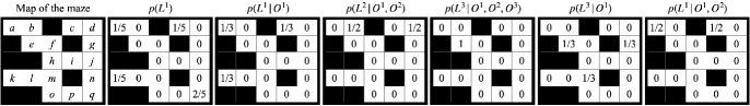
Figure 4: A map of the maze and probability distributions over robot locations, where $O^{1}=1011$, $O^{2}=1100$ and $O^{3}=0011$.

Consider a robot located somewhere in the maze shown on the leftmost panel in Figure 4. The task of the robot is to find its location in the maze only using potentially noisy data coming from its sensors that detect obstacles in the north, east, south and west neighbour rooms.

We assume propositional atoms $N,E,S,W\in{\cal L}$ to represent the presence (1) or absence (0) of obstacles in the north, east, south and west, respectively. The propositional atom $L_{x}\in{\cal L}$ represents the presence (1) or absence (0) of the robot in $x\in\{a,b,...,q\}$. For the sake of simplicity, we use symbol $L$ to represent the location of the robot.

We assume no map of the maze for the robot, which makes the localisation problem in this paper harder than the typical one (?). We instead assume that the robot has potentially noisy data about the maze. The data is assumed to be collected by the robot via its sensors before it is located somewhere in the maze. Suppose the robot has data ${\cal D}=\{\bm{d}_{1}$, $\bm{d}_{2}$, $\bm{d}_{3}$, $\bm{d}_{4}$, $\bm{d}_{5}\}$ where

$$\bm{d}_{1}=((a,1,0,1,1),(b,1,1,0,0),(e,0,0,1,1))$$

$$\bm{d}_{2}=((c,1,0,1,1),(d,1,1,0,0),(g,0,1,0,1))$$

$$\bm{d}_{3}=((k,1,0,1,1),(l,1,0,1,0),(m,0,1,0,0))$$

$$\bm{d}_{4}=((q,0,1,1,0),(p,1,0,1,0),(o,0,0,1,1))$$

$$\bm{d}_{5}=((q,0,1,1,0),(n,0,1,0,1),(j,0,1,0,0)).$$

Here, $d_{k}^{t}$ is a sequence of realisations of $(L^{t}$, $N^{t}$, $E^{t}$, $S^{t}$, $W^{t})$. For simplicity, we assumed no noise in the data. We use symbol $O^{t}$ to denote $(N^{t}$, $E^{t}$, $S^{t}$, $W^{t})$ and omit commas. For example, $d_{1}^{2}=b1100$ means that the robot sensed obstacles only in the north and east in room $b$ at time 2.

Now, given the generative logic $\{p(\bm{\Gamma}|\bm{M},\mu=1)$, $p(\bm{M}|D)$, $p(D)\}$ defined on ${\cal D}$, we can apply the inference tasks we formalised in Section 3.3. We first ask the probability of the current, future and past locations of the robot. The second panel in Figure 4 shows the probability of each robot location at time 1 when the robot perceives nothing at time 1. The distribution is reasonable in terms of ${\cal D}$ because the robot has been to $a$, $c$ and $k$ once, but to $q$ twice at time 1. The third, fourth and fifth panels show examples of prediction discussed in Section 3.3. It is observed that sensory inputs over time help the robot identify its location. The 6th panel shows another example of prediction about a future location, and the 7th shows an example of smoothing.

Given the sensory inputs $O^{1}=1011$, $O^{2}=1100$, $O^{3}=0011$, we have the following most likely explanation.

$$\operatorname*{arg\,max}_{\bm{l}^{1:3}}p(\bm{l}^{1:3}|O^{1}=1011,O^{2}=1100,O^{3}=0011)$$

$$=(L^{1}=a,L^{2}=b,L^{3}=e)$$

The following shows examples of reference, which allows us to refer to the data whose probability distribution is updated in light of sensory inputs.

$$p(D)=\langle 1/5,1/5,1/5,1/5,1/5\rangle$$

$$p(D|O^{1}=1011)=\langle 1/3,1/3,1/3,0,0\rangle$$

$$p(D|O^{1}=1011,O^{2}=1100)=\langle 1/2,1/2,0,0,0\rangle$$

$$p(D|O^{1}=1011,O^{2}=1100,O^{3}=0011)=\langle 1,0,0,0,0\rangle$$

Now, suppose ${\cal D}=\{\bm{d}_{1}$, $\bm{d}_{2}$, $\bm{d}_{3}$, $\bm{d}_{4}$, $\bm{d}_{5}\}$ where $\bm{d}_{1}=(a1011$, $b1100$, $e0011)$, $\bm{d}_{2}=(c1011,d1100,g0101)$, $\bm{d}_{3}=(k1011$, $l1010$, $m0100)$, $\bm{d}_{4}=(q0110$, $p1010$, $o0011)$ and $\bm{d}_{5}=(q0110$, $n0101$, $j0100)$. Given the generative logic $\{p(\bm{\Gamma}|\bm{M},\mu\to 1)$, $p(\bm{M}|D)$, $p(D)\}$ defined on ${\cal D}$, consider that the robot is not aware of the fact that the north and east sensors usually sense the absence of obstacles due to sensor trouble. Let $NESW^{1}(=O^{1})=0011$ and $NESW^{2}(=O^{2})=0000$. No data instantiate the models. Now, we have

$$p(L^{2}|O^{1},O^{2})=\frac{|\langle\!\langle L^{2}\rangle\!\rangle\cap\langle\!\langle O^{1}=0011,O^{2}=0000\rangle\!\rangle^{\prime}|}{|\langle\!\langle O^{1}=0011,O^{2}=0000\rangle\!\rangle^{\prime}|}$$

$$=\frac{|\langle\!\langle L^{2}\rangle\!\rangle\cap\bigcup_{S\in MFS(\{O^{1}=0011,O^{2}=0000\})}\langle\!\langle S\rangle\!\rangle|}{|\bigcup_{S\in MFS(\{O^{1}=0011,O^{2}=0000\})}\langle\!\langle S\rangle\!\rangle|}.$$

$MFS(\{O^{1}=0011,O^{2}=0000\})=\{S_{1},S_{2}\}$ where $S_{1}=\{ESW^{1}=011$, $SW^{2}=00\}$ and $S_{2}=\{ESW^{1}=011$, $EW^{2}=00\}$. We thus have

$$p(L^{2}|O^{1},O^{2})=\frac{|\langle\!\langle L^{2}\rangle\!\rangle\cap(\langle\!\langle S_{1}\rangle\!\rangle\cup\langle\!\langle S_{2}\rangle\!\rangle)|}{|\langle\!\langle S_{1}\rangle\!\rangle\cup\langle\!\langle S_{2}\rangle\!\rangle|}$$

$$=\frac{|\langle\!\langle L^{2}\rangle\!\rangle\cap(\{\bm{d}_{1},\bm{d}_{2}\}\cup\{\bm{d}_{3}\})|}{|\{\bm{d}_{1},\bm{d}_{2}\}\cup\{\bm{d}_{3}\}|}=\frac{|\langle\!\langle L^{2}\rangle\!\rangle\cap\{\bm{d}_{1},\bm{d}_{2},\bm{d}_{3}\}|}{|\{\bm{d}_{1},\bm{d}_{2},\bm{d}_{3}\}|}.$$

Therefore, we have

$$p(L^{2}|O^{1}=0011,O^{2}=0000)=\begin{cases}1/3&\text{ if }L_{2}=b,d,l\\ 0&\text{ otherwise}.\end{cases}$$

Using the previous data without noise, we saw that the robot had a certain belief about its location using the correct sensory inputs. The above result shows that a broken or noisy sensory input is still useful for the robot to reduce the uncertainty of the location.

Suppose that the robot additionally collects another sensory input at time 2. Consider $NESW^{2}(=O^{2})=0100$. To distinguish the first sensory input at time 2 from the second, we write $NESW_{1}^{2}(=O_{1}^{2})=0000$ and $NESW_{2}^{2}(=O_{2}^{2})=0100$. This requires reasoning from inconsistency because $E^{2}=0$ in $O_{1}^{2}$ whereas $E^{2}=1$ in $O_{2}^{2}$. Now, we have

$$p(L^{2}|O^{1},O_{1}^{2},O_{2}^{2})=\frac{|\langle\!\langle L^{2}\rangle\!\rangle\cap\langle\!\langle O^{1},O_{1}^{2},O_{2}^{2}\rangle\!\rangle^{\prime}|}{|\langle\!\langle O^{1},O_{1}^{2},O_{2}^{2}\rangle\!\rangle^{\prime}|}$$

$$=\frac{|\langle\!\langle L^{2}\rangle\!\rangle\cap\bigcup_{S\in MFS(\{O^{1}=0011,O_{1}^{2}=0000,O_{2}^{2}=0100\})}\langle\!\langle S\rangle\!\rangle|}{|\bigcup_{S\in MFS(\{O^{1}=0011,O_{1}^{2}=0000,O_{2}^{2}=0100\})}\langle\!\langle S\rangle\!\rangle|}.$$

$MFS(\{O^{1}=0011,O_{1}^{2}=0000,O_{2}^{2}=0100\})=\{S\}$ where $S=\{ESW^{1}=011$, $SW_{1}^{2}=00$, $ESW_{2}^{2}=100\}$. We thus have

$$p(L^{2}|O^{1},O_{1}^{2},O_{2}^{2})=\frac{|\langle\!\langle L^{2}\rangle\!\rangle\cap\langle\!\langle S\rangle\!\rangle|}{|\langle\!\langle S\rangle\!\rangle|}=\frac{|\langle\!\langle L^{2}\rangle\!\rangle\cap\{\bm{d}_{1},\bm{d}_{2}\}|}{|\{\bm{d}_{1},\bm{d}_{2}\}|}.$$

Therefore, we have

$$p(L^{2}|O^{1},O_{1}^{2},O_{2}^{2})=\begin{cases}1/2&\text{ if }L_{2}=b,d\\ 0&\text{ otherwise}.\end{cases}$$

The above result shows that an inconsistent sensory input is useful for the robot to reduce the uncertainty of the location.

In addition to $NESW^{1}(=O^{1})=0011$, $NESW_{1}^{2}(=O_{1}^{2})=0000$ and $NESW_{2}^{2}(=O_{2}^{2})=0100$ assumed in the previous section, suppose $NESW^{3}(=O^{3})=0011$. Given $\bm{O}^{1:3}$, the most likely explanation is obtained as follows.

$$\operatorname*{arg\,max}_{\bm{l}^{1:3}}p(\bm{l}^{1:3}|\bm{O}^{1:3})=\operatorname*{arg\,max}_{\bm{l}^{1:3}}|\langle\!\langle\bm{l}^{1:3}\rangle\!\rangle\cap\langle\!\langle\bm{O}^{1:3}\rangle\!\rangle^{\prime}|$$

$$=\operatorname*{arg\,max}_{\bm{l}^{1:3}}|\langle\!\langle\bm{l}^{1:3}\rangle\!\rangle\cap\bigcup_{S\in MFS(\bm{O}^{1:3})}\langle\!\langle S\rangle\!\rangle|$$

$MFS(\bm{O}^{1:3})=\{S\}$ where $S=\{ESW^{1}=011$, $SW_{1}^{2}=00$, $ESW_{2}^{2}=100$, $NESW^{3}=0011\}$. We thus have

$$\operatorname*{arg\,max}_{\bm{l}^{1:3}}p(\bm{l}^{1:3}|\bm{O}^{1:3})= \operatorname*{arg\,max}_{\bm{l}^{1:3}}|\langle\!\langle\bm{l}^{1:3}\rangle\!\rangle\cap\langle\!\langle S\rangle\!\rangle|$$

$$= \operatorname*{arg\,max}_{\bm{l}^{1:3}}|\langle\!\langle\bm{l}^{1:3}\rangle\!\rangle\cap\{\bm{d}_{1}\}|.$$

Therefore, we have

$$\operatorname*{arg\,max}_{\bm{l}^{1:3}}p(\bm{l}^{1:3}|\bm{O}^{1:3})=\begin{cases}1&\text{ if }\bm{L}^{1:3}=(a,b,e)\\ 0&\text{ otherwise}.\end{cases}$$

The above result shows that the robot reduced the uncertainty about its location path over time.

Finally, consider the reference $p(D|O^{1},O_{1}^{2})$ where $NESW^{1}(=O^{1})=0011$ and $NESW_{1}^{2}(=O_{1}^{2})=0000$. $MFS(\{O^{1},O^{2}\})=\{S_{1},S_{2}\}$ where $S_{1}=\{ESW^{1}=011$, $SW^{2}=00\}$ and $S_{2}=\{ESW^{1}=011$, $EW^{2}=00\}$. We thus have $\langle\!\langle S_{1}\rangle\!\rangle=\{\bm{d}_{1},\bm{d}_{2}\}$ and $\langle\!\langle S_{2}\rangle\!\rangle=\{\bm{d}_{3}\}$. Therefore,

$$p(D|O^{1},O_{1}^{2})=\begin{cases}\frac{1}{3}&\text{ if }D=\bm{d}_{1},\bm{d}_{2},\bm{d}_{3}\\ 0&\text{ otherwise.}\end{cases}$$

The above result shows that reference tells which stored data the robot should imagine from potentially impossible and inconsistent sensory inputs. The ability of the robot to perform the reference task is thus related to explainable AI.

5 Conclusions

This paper presented a simple theory of inference to reason logically fully from data over time. We showed the statistical and logical correctness of the model and then introduced several inference patterns that are useful to handle temporal inference tasks. The theory was applied to a localisation problem to show that a robot with broken or noisy sensors can efficiently solve the problem in a fully data-driven fashion.

References

• Adams, Huys, and Roiser 2016 Adams, R. A.; Huys, Q. J. M.; and Roiser, J. P. 2016. Computational psychiatry: towards a mathematically informed understanding of mental illness. Journal of Neurology, Neurosurgery & Psychiatry 87(1):53–63.
• Domingos 2015 Domingos, P. 2015. The Master Algorithm: How the Quest for the Ultimate Learning Machine Will Remake Our World. Allen Lane.
• Friedman et al. 1996 Friedman, N.; Getoor, L.; Koller, D.; and Pfeffer, A. 1996. Learning probabilistic relational models. In Proc. 16th Int. Joint Conf. on Artif. Intell., 1297–1304.
• Friston 2010 Friston, K. 2010. The free-energy principle: a unified brain theory? Nature Reviews Neuroscience 11:127–138.
• Hawkins 2021 Hawkins, J. 2021. A Thousand Brains: A New Theory of Intelligence. Basic Books.
• Hohwy 2014 Hohwy, J. 2014. The Predictive Mind. Oxford University Press.
• Itti and Baldi 2009 Itti, L., and Baldi, P. 2009. Bayesian surprise attracts human attention. Vision Research 49(10):1295–1306.
• Kido 2022 Kido, H. 2022. Generative logic models for data-based symbolic reasoning. In Proc. 8th International Workshop on Artificial Intelligence and Cognition, 1–14.
• Knill and Pouget 2004 Knill, D. C., and Pouget, A. 2004. The bayesian brain: the role of uncertainty in neural coding and computation. Trends in Neurosciences 27:712–719.
• Knill and Richards 1996 Knill, D. C., and Richards, W. 1996. Perception as Bayesian Inference. Cambridge University Press.
• Mountcastle 1982 Mountcastle, V. B. 1982. An organizing principle for cerebral function: the unit module and the distributed system. MIT Press, revised ed. edition edition. 7–50.
• Nienhuys-Cheng and Wolf 1997 Nienhuys-Cheng, S. H., and Wolf, R. D. 1997. Foundation of Inductive Logic Programming. Springer.
• Pearl 1988 Pearl, J. 1988. Probabilistic Reasoning in Intelligent Systems: Networks of Plausible Inference. Morgan Kaufmann.
• Pellicano and Burr 2012 Pellicano, E., and Burr, D. 2012. When the world becomes ’too real’: a bayesian explanation of autistic perception. Trends in Cognitive Sciences 16(10):504–510.
• Rao and Ballard 1999 Rao, R. P. N., and Ballard, D. H. 1999. Predictive coding in the visual cortex: a functional interpretation of some extra-classical receptive-field effects. Nature Neuroscience 2:79\UTF201387.
• Richardson and Domingos 2006 Richardson, M., and Domingos, P. 2006. Markov logic networks. Machine Learning 62:107–136.
• Russell and Norvig 2020 Russell, S., and Norvig, P. 2020. Artificial Intelligence : A Modern Approach, Fourth Edition. Pearson Education, Inc.
• Sanborn and Chater 2016 Sanborn, A. N., and Chater, N. 2016. Bayesian brains without probabilities. Trends in Cognitive Sciences 20:883–893.
• Sato 1995 Sato, T. 1995. A statistical learning method for logic programs with distribution semantics. In Proc. 12th int. conf. on logic programming, 715–729.
• von Melchner, Pallas, and Sur 2000 von Melchner, L.; Pallas, S. L.; and Sur, M. 2000. Visual behaviour mediated by retinal projections directed to the auditory pathway. Nature 404(6780):871–876.