Inflation in $f(R,T)$ gravity with observational constraints

Abstract

The scenario of slow-roll inflation is explored in the $f(R,T)$ theory of gravity where a non-minimal coupling between matter and curvature is included. A noncanonical scalar field is assumed to play the role of inflaton which contains generalized kinetic energy. The study is performed by taking the Hamilton-Jacobi formalism where the Hubble parameter is taken as a function of the scalar field. In this regard, a power-law function and an exponential function of the scalar field are assumed for the Hubble parameter and the model is considered in detail. By performing Python coding and applying the observational data, the free parameters of the model are determined for which the model is put in perfect consistency with the data. Then, using the results, the validity of the swampland criteria and TCC is considered. It is realized that not only the model comes to a good agreement with data, but it also could satisfy the swampland criteria.

I Introduction

Although the theory of general relativity has emerged successfully from many experiments, some challenging issues cannot be solved in the frame of general relativity. One of the main issues that the theory is faced with is the flatness and horizon problems. It could not provide a competent explanation for the problems. A possible solution is assuming an early exponential expansion phase, known as cosmic inflation, which has been developed by many scientists Albrecht and Steinhardt (1982); Linde (1982, 1983) since its first introduction Starobinsky (1980); Guth (1981). A common approach for studying inflation is by considering a single scalar field, known as inflaton, with a potential and imposing the slow-roll approximations Linde (2000, 1990, 2005a, 2005b); Riotto (2003); Baumann (2011); Weinberg (2008); Lyth and Liddle (2009); Liddle and Lyth (2000). The scenario shows an incredible consistency with data and it becomes the cornerstone of any cosmological model Ade et al. (2014, 2016); Akrami et al. (2018). There are many different models of inflation based on the aforementioned suggestions Barenboim and Kinney (2007); Franche et al. (2010); Unnikrishnan et al. (2012); Rezazadeh et al. (2015); Saaidi et al. (2015); Fairbairn and Tytgat (2002); Mukohyama (2002); Feinstein (2002); Padmanabhan (2002); Aghamohammadi et al. (2014); Spalinski (2007); Bessada et al. (2009); Weller et al. (2012); Nazavari et al. (2016); Maeda and Yamamoto (2013); Abolhasani et al. (2014); Alexander et al. (2015); Tirandari et al. (2018); Maartens et al. (2000); Golanbari et al. (2014a); Mohammadi et al. (2022a, 2021a, 2017, 2015); Berera (1995, 2000); Hall et al. (2004); Sayar et al. (2017); Akhtari et al. (2017); Sheikhahmadi et al. (2019); Mohammadi et al. (2020a, 2018, 2019); Golanbari et al. (2020a); Mohammadi et al. (2020b, c, 2021b); Mohammadi (2021, 2022); Mohammadi et al. (2022b).

Another issue that the general theory of relativity encounters is the requirement of dark energy and dark matter to be able to fit the cosmological data. This issue became the main motivation for introducing alternative theories of gravity Golanbari et al. (2020b, 2015, 2014b); Aghamohammadi et al. (2013); Saa ; Saaidi and Mohammadi (2012); Saaidi et al. (2012, 2011); Saaidi and Mohammadi (2010). The $f(R,T)$ gravity theory is one of the alternative theories where $R$ is the curvature scalar, $T$ is the trace of the energy-momentum tensor, and $f$ is an arbitrary function of $R$ and $T$. The theory was first introduced by Harko et. al. Harko et al. (2011). It has been utilized to study different topics in cosmology including dark energy Bhatti and Yousaf (2016), dark matter Zaregonbadi et al. (2016), wormholes Moraes and Sahoo (2019), gravitational waves Alves et al. (2016). The theory has also been used to investigate inflationary phase Bhattacharjee et al. (2020); Gamonal (2021), however, it has less attention in this area compared to other modified gravity theories such as $f(R)$ theory and scalar-tensor theory. Most of these works only considered the canonical scalar field, and no work has been done using other fields such as the noncanonical scalar field which could be addressed as a subclass of the k-essence scalar field.

Investigating single-field noncanonical inflation in $f(R,T)$ gravity theory is the main aim that we are going to pursue. The work is followed using Hamilton-Jacobi formalism and for some types of Hubble parameters in detail. The free parameters are determined by using observational data. Besides the observational constraints, there are some theoretical constraints for inflationary models. One of these constraints is the swampland criteria which has been introduced recently in Obied et al. (2018); Ooguri et al. (2019) and refined in Garg and Krishnan (2019). The swampland criteria include two conjectures: first, the range of the inflationary field should satisfy the condition $\Delta\phi/M_{p}<c_{1}$, and the second conjecture concerns the gradient of the potential which is $M_{p}V^{\prime}/V>c_{2}$ (where both $c_{1}$ and $c_{2}$ are constants of the order of one) Kehagias and Riotto (2018). The other constraint is the trans-Planckian censorship conjecture (TCC) Bedroya and Vafa (2020). The conjecture states that no fluctuation with a wavelength less than the Planck length could cross the horizon, freeze, become classical, and lose its quantum nature. The conjecture puts a strong condition on the energy scale of inflation and the tensor-to-scalar ratio and only a few models could survive Bedroya et al. (2020); Brandenberger and Wilson-Ewing (2020).
The paper is organized as follows: the theory and its main dynamics equations are briefly introduced in Sec.II. In Sec.III, the noncanonical scalar field is brought up as the inflaton and the dynamical equations are rewritten under the approximations. Then the perturbation parameters are introduced. The model is considered in detail for some examples of the Hubble parameter in Sec.IV. Using data and by performing coding in Python, the free parameters of the model are determined. The swampland criteria and TCC are considered in Secs.V. Finally, the results are summarized in Sec.VI.

II Basic equations in $f(R,T)$ gravity

The general action in $f(R,T)$ gravity theory is given as follows

$$S={1\over 2\kappa^{2}}\;\int d^{4}x\sqrt{-g}\;\Big{(}f(R,T)+\mathcal{L}_{m}\Big{)}$$ (1)

where $\kappa$ is defined as $\kappa^{2}=8\pi G$ and $G$ is the Newtonian gravitational constant. $R$ is the Ricci scalar constructed from the metric $g_{\mu\nu}$ with determinant $g$. The second term in the parenthesis, $\mathcal{L}_{m}$ is the Lagrangian of the matter field. $T$ is the determinant of the energy-momentum tensor $T_{\mu\nu}$ and $f(R,T)$ is an arbitrary function of $R$ and $T$.
The field equation of the theory is obtained by taking a variation of the above action with respect to the metric, which is read as

$$\Xi_{\mu\nu}f_{,R}(R,T)+f_{,R}R_{\mu\nu}-{1\over 2}g_{\mu\nu}f(R,T)=\kappa^{2}T_{\mu\nu}-f_{,T}(R,T)\big{(}T_{\mu\nu}+\Theta_{\mu\nu}\big{)},$$ (2)

where the operator $\Xi_{\mu\nu}$ and $\Theta_{\mu\nu}$ are respectively defined as

$$\Xi_{\mu\nu} = g_{\mu\nu}\square-\nabla_{\mu}\nabla_{\nu},$$ (3)

$$\Theta_{\mu\nu} = g^{\alpha\beta}{\delta T_{\alpha\beta}\over\delta g^{\mu\nu}}.$$ (4)

The energy-mometum tensor is assumed to be played by a perfect fluid with the following form

$$T_{\mu\nu}=(\rho+p)u_{\mu}u_{\nu}-pg_{\mu\nu}$$ (5)

where $\rho$ and $p$ are the energy density and pressure of the fluid.
To go further, $f(R,T)$ is picked out as $f(R,T)=R+\eta T$, where $\eta$ is a constant. This choice for $f(R,T)$ is one of the simplest and most common choices which has been studied in different topics Harko et al. (2011); Moraes et al. (2016); Carvalho et al. (2017); Moraes et al. (2019); Moraes and Sahoo (2017); Moraes et al. (2017); Azizi (2013); Moraes (2014, 2015); Reddy and Santhi Kumar (2013). Taking a spatially flat FLRW metric, the friedmann equations are obtained as Bhattacharjee et al. (2020)

$$H^{2} = {\kappa^{2}\over 3}\;\left(\big{(}{3\over 2}\lambda+1\big{)}\;\rho-{\lambda\over 2}\;p\right),$$ (6)

$$-3H^{2}-2\dot{H} = \kappa^{2}\left(-{\lambda\over 2}\;\rho+\big{(}{3\over 2}\lambda+1\big{)}\;p\right),$$ (7)

where the constant $\lambda$ comes from the definition $\eta=\lambda\kappa^{2}$. Combining these two equations, the time derivative of the Hubble parameter is acquired

$$-2\dot{H}=\kappa^{2}\;(1+\lambda)\;(\rho+p).$$ (8)

The consevation equation is obtained by taking the time derivative from Eq.(6) and using Eq.(8) as

$$\left({3\lambda\over 2}+1\right)\;\dot{\rho}-{\lambda\over 2}\;\dot{p}+3H\;(1+\lambda)\;(\rho+p)=0.$$ (9)

All above equations return to the standard ones by imposing $\lambda=0$.

III Noncanonical inflation

The Lagrangian of the noncanonical scalar field is given by

$$\mathcal{L}(\phi,X)=X\left({X\over M^{4}}\right)^{\alpha-1}-V(\phi)$$ (10)

where $X=\dot{\phi}^{2}/2$. It returns to the canonical inflation for $\alpha=1$. The related energy density and pressure are

$$\rho = (2\alpha-1)X\left({X\over M^{4}}\right)^{\alpha-1}+V(\phi)$$

$$p = X\left({X\over M^{4}}\right)^{\alpha-1}-V(\phi).$$ (11)

Substituting the above energy density and pressure in the Friedmann equation (6) and (8), one arrives at

$$H^{2} = {1\over 3M_{p}^{2}}\;\left[\left(2\alpha\Big{(}{3\lambda\over 2}+1\Big{)}-\big{(}1+2\lambda\big{)}\right)\;\left({X\over M^{4}}\right)^{\alpha-1}X+(1+2\lambda)\;V(\phi)\right]$$

$$\dot{H} = {-1\over 2M_{p}^{2}}\;(1+\lambda)\;2\alpha\;\left({X\over M^{4}}\right)^{\alpha-1}X.$$ (12)

The field equation of motion is obtained by substituting Eqs.(11) in the modified conservation equation (9), read as

$$\left(2\alpha\Big{(}{3\lambda\over 2}+1\Big{)}-\big{(}1+2\lambda\big{)}\right)\;\ddot{\phi}+3H\big{(}1+2\lambda\big{)}\;\dot{\phi}+{1\over\alpha}\;\left({M^{4}\over X}\right)^{\alpha-1}\;V^{\prime}(\phi)=0$$ (13)

where prime indicates derivatives with respect to the field. For $\alpha=1$ and $\lambda=0$, the usual field equation for canonical scalar field is recovered.

III.1 Hamilton-Jacobi formalism

Following the Hamilton-Jacobi formalism, the Hubble parameter instead of the potential is introduced in terms of the scalar field, $H=H(\phi)$. Then, the time derivative of the Hubble parameter is rewritten as $\dot{H}=\dot{\phi}H^{\prime}(\phi)$. Using it in Eq.(12), one has

$$H^{\prime}(\phi)={\alpha(1+\lambda)\over M_{p}^{2}\xi}\;X^{\alpha}\;{-1\over\dot{\phi}}$$ (14)

where the constant $\xi$ is defined as $\xi=M^{4(\alpha-1)}$. The above equation is utilized to read $\dot{\phi}$ in terms of the Hubble parameter.
Reading the Kinetic term $X$ from Eq.(12) and substituting it in the Friedmann equation, the potential is given as

$$V(\phi)={3M_{p}^{2}\over(1+2\lambda)}\;H^{2}\left[1+{2\alpha\Big{(}{3\lambda\over 2}+1\Big{)}-\big{(}1+2\lambda\big{)}\over 3\alpha(1+\lambda)}\;\epsilon_{1}\right],$$ (15)

which is addressed as the Hamilton-Jacobi equation. The parameter $\epsilon_{1}$ in the above equation is known as the first slow-roll parameter defined as

$$\epsilon_{1}={-\dot{H}\over H^{2}}=\left({2^{\alpha}M_{p}^{2}\xi\over\alpha(1+\lambda)}\right)^{1\over 2\alpha-1}\;{H^{\prime}{}^{2\alpha\over 2\alpha-1}\over H^{2}}.$$ (16)

The second slow-roll parameter is defined through a hierarchy approach as

$$\epsilon_{2}={\dot{\epsilon}_{1}\over H\epsilon_{1}}=2\;\epsilon_{1}-2\alpha\;\eta_{H}$$ (17)

where

$$\eta_{H}={1\over 2\alpha-1}\;\left({2^{\alpha}M_{p}^{2}\xi\over\alpha(1+\lambda)}\right)^{1\over 2\alpha-1}\;{H^{\prime}{}^{2-2\alpha\over 2\alpha-1}H^{\prime\prime}\over H}.$$ (18)

The amount of inflation is important for solving the problem of the hot big bang theory. The amount of inflation is measured by the parameter number of e-folds given by

$$N=\int_{t_{\star}}^{t_{e}}H\;dt=\int_{\phi_{\star}}^{\phi_{e}}$$ (19)

where $"\star"$ and $"e"$ stand for the horizon crossing time and end of inflation.

III.2 Perturbations

To verify the validity of any inflationary model, it is required to compare the predictions of the model with observational data. In the following lines, we are going to introduce some of these perturbation parameters which are essential for us in the next section where the model is considered for some specific types of potentials. One of the important parameters is the amplitude of the scalar perturbations which is given by

$$\mathcal{P}_{s}={1\over 4\pi^{2}}\;{H^{4}\over c_{s}\big{(}\rho_{eff}+p_{eff}\big{)}}$$ (20)

where

$$\rho_{eff} = \left(\big{(}{3\over 2}\lambda+1\big{)}\;\rho-{\lambda\over 2}\;p\right)$$

$$p_{eff} = \left(-{\lambda\over 2}\;\rho+\big{(}{3\over 2}\lambda+1\big{)}\;p\right)$$

with $\rho$ and $p$ are the energy density and pressure of the noncanonical scalar field given by Eq.(11). The sound speed $c_{s}$ is obtained as

$$c_{s}^{2}={\dot{p}_{eff}\over\dot{\rho}_{eff}}={(1+2\lambda)-\alpha\lambda\over 2\alpha\Big{(}{3\lambda\over 2}+1\Big{)}-\big{(}1+2\lambda\big{)}}.$$ (21)

which is constant.
The scalar spectral index, which is defined through the amplitude of the scalar field, is given by

$$n_{s}=1-(2\epsilon_{1}+\epsilon_{2}).$$ (22)

Regarding the tensor perturbations, there is the tensor-to-scalar ratio which is very essential in examining an inflationary model. The parameter is expressed as follows

$$r=16\;c_{s}\;\epsilon_{1}.$$ (23)

In the following section, we are going to examine the model for some specific types of potential and compare the results with the data.

IV Typical examples

In this section, three types of potentials as power-law, T-mode, and exponential will be studied in detail.

IV.1 power-law case

In the first case, the Hubble parameter is taken as a power-law function of the scalar field, $H(\phi)=H_{0}\phi^{n}$ where $H_{0}$ and $n$ are two constants. Using this definition, the slow-roll parameters are

$$\epsilon_{1} = \left({2^{\alpha}M_{p}^{2}\xi\over\alpha(1+\lambda)}\;n^{2\alpha}\;H_{0}^{2-2\alpha}\right)^{1\over 2\alpha-1}\;\phi^{2n-2n\alpha-2\alpha\over 2\alpha-1}$$ (24)

$$\eta_{H} = {n(n-1)\over 2\alpha-1}\;\left({2^{\alpha}M_{p}^{2}\xi\over\alpha(1+\lambda)}\;n^{2-2\alpha}\;H_{0}^{2-2\alpha}\right)^{1\over 2\alpha-1}\;\phi^{2n-2n\alpha-2\alpha\over 2\alpha-1}$$ (25)

Inflation ends as the first slow-roll parameter reaches one, $\epsilon_{1}=1$. The scalar field at the end of inflation is read from this relation which is

$$\phi_{e}^{2n-2n\alpha-2\alpha\over 2\alpha-1}=\left({2^{\alpha}M_{p}^{2}\xi\over\alpha(1+\lambda)}\;n^{2\alpha}\;H_{0}^{2-2\alpha}\right)^{-1\over 2\alpha-1}$$ (26)

We are going to determine the free parameters of the model by comparing its results with observational data. In this regard, we need to estimate the perturbation parameters at the time of horizon crossing. First, the scalar field is computed through the relation of the number of e-folds as

$$\phi_{\star}^{2n-2n\alpha-2\alpha\over 2\alpha-1}=\left[\left({2^{\alpha}M_{p}^{2}\xi\over\alpha(1+\lambda)}\;n^{2\alpha}\;H_{0}^{2-2\alpha}\right)^{1\over 2\alpha-1}\;\left(1-{2n-2n\alpha-2\alpha\over n(2\alpha-1)}\;N\right)\right]^{-1}$$ (27)

Inserting $\phi_{\star}$ in the slow-roll parameters (16) and (17), one arrives at

$$\epsilon_{1}^{\star} = \left(1-{2n-2n\alpha-2\alpha\over n(2\alpha-1)}\;N\right)^{-1},$$ (28)

$$\eta_{H}^{\star} = {(n-1)\over n(2\alpha-1)}\;\left(1-{2n-2n\alpha-2\alpha\over n(2\alpha-1)}\;N\right)^{-1},$$ (29)

and returning to Eqs.(22) and (23), the scalar spectral index and the tensor-to-scalar ratio are obtained at horizon crossing.

(a)

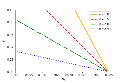
(b)

Figure 1: The $r-n_{s}$ curves in terms of a) $\alpha$ and different values of $n$, b) $n$ for different values of $\alpha$. The constant $\lambda$ is taken as $\lambda=2$ and the curves are plotted for the number of e-folds $N=65$.

Fig.1(a) illustrates $r-n_{s}$ curves versus the parameter $\alpha$ for different values of $\lambda$. It is realized that the curve for $n=0.5$ and $1$ is out of the observational range and it enters the range for $n=1.5$ and $2$. The curves enter the observational range for higher values of $\alpha$ and they are out of range for smaller $\alpha$. The $r-n_{s}$ curves versus $n$ are plotted in Fig.1(b) for different values of $\alpha$. It seems that the curves start from the same point and tend toward the smaller $n_{s}$ and bigger $r$ by increasing $\alpha$. It is realized that the curves related to $\alpha=1$ and $1.5$ do not cross our interest area. On the other hand, the curves related to $\alpha=2$ and $2.4$ perfectly cross the observational area.

Figure 2: The figure illustrates the parametric space of the parameter $\alpha$ and $n$ so that for each point in the parameter the model remains in perfect agreement with the data.

To have a better view of the valid values of free parameters $n$ and $\alpha$, a parametric space is depicted in Fig.2. The blue area indicates a set of $(\alpha,n)$ points for which the model comes to good agreement with the data.

$\alpha$	$n$	$n_{s}$	$r$	$M$	ES
$1.5$	$1.0$	$0.9695$	$0.0653$	$2.29\times 10^{-12}$	$4.47\times 10^{-3}$
$1.5$	$1.5$	$0.9645$	$0.0868$	$5.70\times 10^{-10}$	$4.80\times 10^{-3}$
$1.5$	$2.0$	$0.9605$	$0.1040$	$7.98\times 10^{-9}$	$5.02\times 10^{-3}$
$2.0$	$1.0$	$0.9695$	$0.0368$	$1.23\times 10^{-9}$	$3.88\times 10^{-3}$
$2.0$	$1.5$	$0.9652$	$0.0472$	$5.35\times 10^{-8}$	$4.12\times 10^{-3}$
$2.0$	$2.0$	$0.9620$	$0.0550$	$3.25\times 10^{-7}$	$4.28\times 10^{-3}$
$2.4$	$1.0$	$0.9695$	$0.0145$	$4.59\times 10^{-9}$	$3.07\times 10^{-3}$
$2.4$	$1.5$	$0.9655$	$0.0183$	$1.33\times 10^{-7}$	$3.25\times 10^{-3}$
$2.4$	$2.0$	$0.9626$	$0.0211$	$6.68\times 10^{-7}$	$3.37\times 10^{-3}$

Table 1: The numerical results for the case about the scalar spectral index, tensor-to-scalar ratio, constant $M$, and energy scale (ES) of inflation for different values of $\alpha$ and $n$ taken from Fig.2, where the number of e-folds is $N=65$.

There are exact data about the amplitude of the scalar perturbations as well. Estimating the amplitude of the scalar perturbations at the time of the horizon crossing and applying the data for $\mathcal{P}_{s}$, one could determine other free parameters of the model that is

$$\xi^{2n}={1\over H_{0}^{4\alpha}}\;\left(\left[{\alpha(1+\lambda)\over 2^{\alpha}M_{p}^{2}}\right]^{1\over 2\alpha-1}{\epsilon_{1}^{\star}\over n^{2\alpha\over 2\alpha-1}}\right)^{2n(2\alpha-1)}\;\left({1\over 8\pi^{2}M_{p}^{2}c_{s}\epsilon_{1}^{\star}\mathcal{P}_{s}}\right)^{2n-2n\alpha-2\alpha}$$ (30)

Table.1 presents a brief results of the case and gives a better insight about the case. One could finds the model results for the scalar spectral index, the tensor-to-scalar ratio, the inflation energy scale and also anothe free parameters of the model $M$. These results are computed for different values of $\alpha$ and $n$ so that some of them stand in the blue range of Fig.2 and some do not.

IV.2 Exponential case

The exponential function of the scalar field is picked out as the second case for the Hubble parameter, i.e. $H(\phi)=H_{0}\exp(\beta\phi)$ where $H_{0}$ and $\beta$ are two constant. Substituting this Hubble parameter in Eqs.(16) and (18), the slow-roll parameters are obtained as

$$\epsilon_{1} = \left({2^{\alpha}M_{p}^{2}\xi\over\alpha(1+\lambda)}\;\beta^{2\alpha}\;H_{0}^{2-2\alpha}\right)^{1\over 2\alpha-1}\;e^{{2-2\alpha\over 2\alpha-1}\;\beta\phi},$$ (31)

$$\eta_{H} = {1\over 2\alpha-1}\;\left({2^{\alpha}M_{p}^{2}\xi\over\alpha(1+\lambda)}\;\beta^{2\alpha}\;H_{0}^{2-2\alpha}\right)^{1\over 2\alpha-1}\;e^{{2-2\alpha\over 2\alpha-1}\;\beta\phi}.$$ (32)

Solving the relation $\epsilon_{1}=1$ in terms of $\phi$, the field is estimated at the end of inflation

$$e^{{2\alpha-2\over 2\alpha-1}\;\beta\;\phi_{e}}=\left({2^{\alpha}M_{p}^{2}\xi\over\alpha(1+\lambda)}\;\beta^{2\alpha}\;H_{0}^{2-2\alpha}\right)^{1\over 2\alpha-1}.$$ (33)

Applying this result on Eq.(19) and by integrating, the field at the time of the horizon crossing is given by

$$e^{{2\alpha-2\over 2\alpha-1}\;\beta\;\phi_{\star}}=e^{{2\alpha-2\over 2\alpha-1}\;\beta\;\phi_{\star}}\left(1+{2\alpha-2\over 2\alpha-1}\;N\right).$$ (34)

To estimate the scalar spectral index and the tensor-to-scalar ratio at the time of the horizon crossing, we first need to substitute the above field in the slow-roll parameters which leads to

$$\epsilon_{1}^{\star} = \left(1+{2\alpha-2\over 2\alpha-1}\;N\right)^{-1}$$ (35)

$$\eta_{H}^{\star} = {1\over 2\alpha-1}\;\epsilon_{1}^{\star}.$$ (36)

Using the slow-roll parameters in Eq.(22) and (23), $n_{s}$ and $r$ are obtained at $t_{\star}$. The behavior of the parameters is described in Fig.3, where one finds $r-n_{s}$ curves versus the parameter $\alpha$ for different values of $\lambda$. For smaller values of $\lambda$, the curves come to the observational range for larger values of $\alpha$.

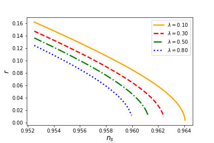
Figure 3: The $r-n_{s}$ curves in terms of the $\alpha$ for different values of $\lambda$ where the number of e-fold is $N=85$.

In order to have a better understanding about the valid range of the parameters $\alpha$ and $\lambda$, we are going to run a Python code including the data for the scalar spectral index and the tensor-to-scalar ratio. The resulted parametric space is presented in Fig.4 that shows a set of $(\alpha,\lambda)$ for which the model is kept consistent with data. Also, one realizes that there is bigger range of $\lambda$ for smaller values of $\alpha$.

Figure 4: The figure portrays a oarametric space for the free parameters $\alpha$ and $\lambda$ where the number of e-folds is $N=85$. For each point in the space the model comes to an agreement with data.

Using the data about the amplitude of the scalar perturbations, another free parameter of the model is determined. From Eq.(20), it is found that

$$\xi={\alpha(1+\lambda)\over 2^{\alpha}M_{p}^{2}}\;{\epsilon_{1}^{2\alpha-1}\over\big{(}8\pi^{2}M_{p}^{2}c_{s}\epsilon_{1}\mathcal{P}_{s}\big{)}^{1-\alpha}\beta^{2\alpha}}$$ (37)

Table.2 represents the value of the constant $M=\xi^{1/4(\alpha-1)}$ for different choices of $\alpha$ and $\lambda$. The magnitude of the free parameter $M$ is about $\mathcal{O}(10^{5})$. Moreover, for each $\alpha$ and $\lambda$, the scalar spectral index, the tensor-to-scalar ration, and the energy scale of inflation are given as well. It is seen that the scalar spectal index and the tensor-to-scalar ratio stand in agreement with data. The enegy scale of inflation also increase by enhancement of $\alpha$.

$\alpha$	$\lambda$	$n_{s}$	$r$	$\xi$	ES
$3.5$	$0.1$	$0.9606$	$0.0785$	$7.10\times{-5}$	$1.03\times{-2}$
$3.5$	$0.2$	$0.9606$	$0.0672$	$6.89\times{-5}$	$9.84\times{-3}$
$3.5$	$0.3$	$0.9606$	$0.0565$	$6.65\times{-5}$	$9.44\times{-3}$
$4.0$	$0.1$	$0.9613$	$0.0685$	$7.85\times{-5}$	$4.12\times{-2}$
$4.0$	$0.2$	$0.9613$	$0.0559$	$7.51\times{-5}$	$3.94\times{-2}$
$4.0$	$0.3$	$0.9613$	$0.0433$	$7.06\times{-5}$	$3.78\times{-2}$
$4.5$	$0.1$	$0.9619$	$0.0608$	$8.37\times{-5}$	$1.11\times{-1}$
$4.5$	$0.2$	$0.9619$	$0.0468$	$7.89\times{-5}$	$1.06\times{-1}$
$4.5$	$0.3$	$0.9619$	$0.0314$	$7.18\times{-5}$	$1.02\times{-1}$
$5.0$	$0.1$	$0.9623$	$0.0545$	$8.74\times{-5}$	$2.34\times{-1}$
$5.0$	$0.2$	$0.9623$	$0.0388$	$8.07\times{-5}$	$2.23\times{-1}$
$5.0$	$0.3$	$0.9623$	$0.0184$	$6.73\times{-5}$	$2.15\times{-1}$

Table 2: The numerical results for the scalar spectral index, tensor-to-scalar ratio, constant $M$, and the energy scale (ES) of inflation for different values of $\alpha$ and $\lambda$ where the number of e-folds is $N=85$.

V Swampland criteria and TCC

String theory, which is known as one of the promising candidates for the ultimate theory of quantum gravity, propounds a landscape that contains all consistent low-energy EFTs. Moreover, there are other low-energy EFTs that do not get along with string theory living in an area known as swampland. We desire to build our model based on a consistent low-energy EFT. Therefore, a mechanism is required to separate the consistent and inconsistent theories. over the past years, several conjectures have been introduced in this matter and the most recent conjectures, which are known as swampland criteria, are

• Distance conjecture: it puts an upper bound on the scalar field excursion in the field space

  $$\Delta\phi\leq c_{1}$$ (38)

  where $c_{1}$ is a constant of the order of one, $\mathcal{O}(1)$ Obied et al. (2018); Garg and Krishnan (2019); Ooguri et al. (2019).

• de Sitter conjecture: it stated that there should be a lower bound on the gradient of the potential as Garg and Krishnan (2019); Ooguri et al. (2019)

  $${|V_{,\phi}|\over V}\geq c_{2},$$ (39)

  or as in the refined version of this criterion, one of the following conditions should be satisfied

  $${|V_{,\phi}|\over V}\geq c_{2},\quad{\rm or}{|V_{,\phi\phi}|\over V}\geq-c^{\prime}_{2}$$ (40)

  The true order of the constant $c_{1}$ depends on the detail of compaction. It is concluded that it is larger than $\sqrt{2}$. However, further consideration indicates that it could be smaller, of the order of $\mathcal{O}(0.1)$ Kehagias and Riotto (2018); Ooguri et al. (2019). In any case, the important criterium is that the constant must be positive.

The conjecture is stated in Planck units, $M_{p}=1$. Due to this belief that inflation occurs at an energy scale below the Planck, it is expected to be described by low-energy EFT. Therefore, it is interesting to consider the validation of the swampland criteria for an inflationary model.
In the previous section, the free parameters of the model are determined using data. Now, we are going to use these results, the scalar field at the horizon crossing and the end of inflation is obtained and one could specify the field excursion and the gradient of the potential. Tables.3 and 4 display the results respectively for the first and second cases.

$\alpha$	$n$	$\Delta\phi$	$V^{\prime}/V$
$1.5$	$1.0$	$1.18\times 10^{-5}$	$1.53\times 10^{5}$
$1.5$	$1.5$	$5.28\times 10^{-4}$	$4.92\times 10^{3}$
$1.5$	$2.0$	$3.35\times 10^{-3}$	$9.84\times 10^{2}$
$2.0$	$1.0$	$8.89\times 10^{-6}$	$2.04\times 10^{5}$
$2.0$	$1.5$	$4.27\times 10^{-4}$	$6.02\times 10^{3}$
$2.0$	$2.0$	$2.80\times 10^{-3}$	$1.15\times 10^{3}$
$2.4$	$1.0$	$5.57\times 10^{-6}$	$3.25\times 10^{5}$
$2.4$	$1.5$	$3.10\times 10^{-4}$	$8.25\times 10^{3}$
$2.4$	$2.0$	$2.19\times 10^{-3}$	$1.46\times 10^{3}$

Table 3: The table shows the results for the field distance and potential gradient of the first case for different values of $\alpha$ and $n$.

$\alpha$	$\lambda$	$\Delta\phi$	$V^{\prime}/V$
$3.5$	$0.1$	$0.4885$	$20.927$
$3.5$	$0.2$	$0.4885$	$20.925$
$3.5$	$0.3$	$0.4885$	$20.923$
$4.0$	$0.1$	$0.4780$	$20.926$
$4.0$	$0.2$	$0.4780$	$20.923$
$4.0$	$0.3$	$0.4780$	$20.921$
$4.5$	$0.1$	$0.4704$	$20.924$
$4.5$	$0.2$	$0.4704$	$20.922$
$4.5$	$0.3$	$0.4704$	$20.920$
$5.0$	$0.1$	$0.4647$	$20.923$
$5.0$	$0.2$	$0.4647$	$20.921$
$5.0$	$0.3$	$0.4647$	$20.919$

Table 4: The table shows the results for the field distance and potential gradient of the second case for different values of $\alpha$ and $\lambda$.

The results clarify that both criteria could be satisfied in both cases. For the first case, for the specific parameter $\alpha$, the field distance gets larger by increasing $\lambda$, however, the potential gradient decreases. Besides, there is a reverse situation for specific values of $\lambda$ so that the field distance gets smaller by enhancement of $\alpha$, while the potential gradient increase. For the second case, where the Hubble parameter is taken as an exponential function of the scalar field, the field distance could be smaller than one and the potential gradient larger. The point that one realizes from the table is that the field distance and the potential gradient are not sensitive to the varying of $\alpha$ and $\lambda$.

Another conjecture which has been proposed recently is TCC. The TCC targets the fluctuations generated during inflation. These fluctuations are the origin of the universe structure. They are stretched with the expansion and cross the horizon, freeze and reenter the horizon after inflation, and today we could observe some of them. The crucial point is that the fluctuations have a quantum nature, however, they lose their nature as cross the horizon and freeze. At this point they become classical. Our main concern is the fluctuations with the origin wavelength less than the Planck length. In this case, if inflation lasts long enough, they stretch and cross the horizon and become classical. This is known as the ”trans-Planckian problem”. TCC states that no fluctuation with a wavelength less than the Planck length should cross the horizon Bedroya and Vafa (2020); Bedroya et al. (2020); Mohammadi et al. (2021a), and it is formulated as

$${l_{p}\over a_{i}}<{H_{f}^{-1}\over a_{f}},$$ (41)

where $l_{p}$ is the Planck length, $H_{f}$ is the Hubble parameter at the end of inflation. $a_{i}$ and $a_{f}$ are the scale factor respectively at the beginning and the end of inflation.
The quantity $H_{f}^{-1}$ for both cases of Sec.IV is of the order of $\mathcal{O}(10^{6})$. On the other hand, the term $a_{f}/a_{i}=e^{N}$ is much higher than this magnitude. It implies that the condition $e^{N}<H_{f}^{-1}$ will never be satisfied.

VI Conclusion

The scenario of slow-roll inflation was considered in the $f(R,T)$ theory of gravity, which is known as a modified theory of gravity where the matter has a non-minimal coupling to the curvature. The inflaton was assumed to be played by a noncanonical scalar field including generalized kinetic energy, which is a subclass of the k-essence scalar field. After briefly reviewing the model and its dynamical equations, the scenario of inflation is considering following Hamilton-Jacobi formalism. In this formalism, the Hubble parameter is introduced as a function of the scalar field instead of the potential. The investigation was pursued by considering two cases for the Hubble parameter as power-law and exponential functions of the scalar field. Utilizing observational data and performing a coding program, the free parameters of the model were determined.
First, the Hubble parameter was assumed to be a power-law function of the scalar field. By estimating the scalar field at the time of the horizon crossing, we could compute the main perturbation parameters at this time. Next, by applying the data for the scalar spectral index and the tensor-to-scalar ratio, we could determine the valid range for the free parameters $\alpha$ and $n$. Then, the free parameter $M$ was determined through the amplitude of the scalar perturbations. Following the obtained information about the free parameters of the model, the energy scale of inflation was computed that was of the order of $10^{-3}M_{p}$. Also, we considered the validity of the swampland criteria and TCC. Concerning the swampland criteria, the result implies that the two conjectures are perfectly satisfied. However, the TCC is not satisfied.
In the next case, the Hubble parameter was picked as the exponential function of the scalar field. The same procedure was followed to determine the free parameters of the model for which to put the model in perfect agreement with the data. For the determined free parameters, the model could satisfy the swampland criteria, however, in contrast to the first case, they were not sensitive to the changes of the parameter $\lambda$.

References

- Albrecht and Steinhardt (1982) A. Albrecht and P. J. Steinhardt, Physical Review Letters 48, 1220 (1982).
- Linde (1982) A. D. Linde, Physics Letters B 108, 389 (1982).
- Linde (1983) A. D. Linde, Physics Letters B 129, 177 (1983).
- Starobinsky (1980) A. A. Starobinsky, Physics Letters B 91, 99 (1980).
- Guth (1981) A. H. Guth, Phys. Rev. D23, 347 (1981), [Adv. Ser. Astrophys. Cosmol.3,139(1987)].
- Linde (2000) A. D. Linde, Phys. Rept. 333, 575 (2000).
- Linde (1990) A. D. Linde, Contemp. Concepts Phys. 5, 1 (1990), arXiv:hep-th/0503203 [hep-th] .
- Linde (2005a) A. D. Linde, Proceedings, 6th UCLA Symposium on Sources and Detection of Dark Matter and Dark Energy in the Universe: Marina del Rey, CA, USA, February 18-20, 2004, New Astron. Rev. 49, 35 (2005a).
- Linde (2005b) A. D. Linde, Proceedings, Nobel Symposium 127 on String theory and cosmology: Sigtuna, Sweden, August 14-19, 2003, Phys. Scripta T117, 40 (2005b), arXiv:hep-th/0402051 [hep-th] .
- Riotto (2003) A. Riotto, Astroparticle physics and cosmology. Proceedings: Summer School, Trieste, Italy, Jun 17-Jul 5 2002, ICTP Lect. Notes Ser. 14, 317 (2003), arXiv:hep-ph/0210162 [hep-ph] .
- Baumann (2011) D. Baumann, in Physics of the large and the small, TASI 09, proceedings of the Theoretical Advanced Study Institute in Elementary Particle Physics, Boulder, Colorado, USA, 1-26 June 2009 (2011) pp. 523–686, arXiv:0907.5424 [hep-th] .
- Weinberg (2008) S. Weinberg, Cosmology (2008).
- Lyth and Liddle (2009) D. H. Lyth and A. R. Liddle, The primordial density perturbation: Cosmology, inflation and the origin of structure (2009).
- Liddle and Lyth (2000) A. R. Liddle and D. H. Lyth, Cosmological inflation and large scale structure (2000).
- Ade et al. (2014) P. A. R. Ade et al. (Planck), Astron. Astrophys. 571, A22 (2014), arXiv:arXiv:1303.5082 [astro-ph.CO] .
- Ade et al. (2016) P. A. R. Ade et al. (Planck), Astron. Astrophys. 594, A20 (2016), arXiv:arXiv:1502.02114 [astro-ph.CO] .
- Akrami et al. (2018) Y. Akrami et al. (Planck), (2018), arXiv:arXiv:1807.06211 [astro-ph.CO] .
- Barenboim and Kinney (2007) G. Barenboim and W. H. Kinney, JCAP 0703, 014 (2007), arXiv:astro-ph/0701343 [astro-ph] .
- Franche et al. (2010) P. Franche, R. Gwyn, B. Underwood, and A. Wissanji, Phys. Rev. D82, 063528 (2010), arXiv:1002.2639 [hep-th] .
- Unnikrishnan et al. (2012) S. Unnikrishnan, V. Sahni, and A. Toporensky, JCAP 1208, 018 (2012), arXiv:1205.0786 [astro-ph.CO] .
- Rezazadeh et al. (2015) K. Rezazadeh, K. Karami, and P. Karimi, JCAP 1509, 053 (2015), arXiv:1411.7302 [gr-qc] .
- Saaidi et al. (2015) K. Saaidi, A. Mohammadi, and T. Golanbari, Adv. High Energy Phys. 2015, 926807 (2015), arXiv:1708.03675 [gr-qc] .
- Fairbairn and Tytgat (2002) M. Fairbairn and M. H. G. Tytgat, Phys. Lett. B546, 1 (2002), arXiv:hep-th/0204070 [hep-th] .
- Mukohyama (2002) S. Mukohyama, Phys. Rev. D66, 024009 (2002), arXiv:hep-th/0204084 [hep-th] .
- Feinstein (2002) A. Feinstein, Phys. Rev. D66, 063511 (2002), arXiv:hep-th/0204140 [hep-th] .
- Padmanabhan (2002) T. Padmanabhan, Phys. Rev. D66, 021301 (2002), arXiv:hep-th/0204150 [hep-th] .
- Aghamohammadi et al. (2014) A. Aghamohammadi, A. Mohammadi, T. Golanbari, and K. Saaidi, Phys. Rev. D90, 084028 (2014), arXiv:1502.07578 [gr-qc] .
- Spalinski (2007) M. Spalinski, JCAP 0705, 017 (2007), arXiv:hep-th/0702196 [hep-th] .
- Bessada et al. (2009) D. Bessada, W. H. Kinney, and K. Tzirakis, JCAP 0909, 031 (2009), arXiv:0907.1311 [gr-qc] .
- Weller et al. (2012) J. M. Weller, C. van de Bruck, and D. F. Mota, JCAP 1206, 002 (2012), arXiv:1111.0237 [astro-ph.CO] .
- Nazavari et al. (2016) N. Nazavari, A. Mohammadi, Z. Ossoulian, and K. Saaidi, Phys. Rev. D93, 123504 (2016), arXiv:1708.03676 [gr-qc] .
- Maeda and Yamamoto (2013) K.-i. Maeda and K. Yamamoto, Journal of Cosmology and Astroparticle Physics 2013, 018 (2013).
- Abolhasani et al. (2014) A. A. Abolhasani, R. Emami, and H. Firouzjahi, Journal of Cosmology and Astroparticle Physics 2014, 016 (2014).
- Alexander et al. (2015) S. Alexander, D. Jyoti, A. Kosowsky, and A. Marcianò, Journal of Cosmology and Astroparticle Physics 2015, 005 (2015).
- Tirandari et al. (2018) M. Tirandari, K. Saaidi, and A. Mohammadi, Phys. Rev. D 98, 043516 (2018).
- Maartens et al. (2000) R. Maartens, D. Wands, B. A. Bassett, and I. P. Heard, Physical Review D 62, 041301 (2000).
- Golanbari et al. (2014a) T. Golanbari, A. Mohammadi, and K. Saaidi, Physical Review D 89, 103529 (2014a).
- Mohammadi et al. (2022a) A. Mohammadi, T. Golanbari, S. Nasri, and K. Saaidi, Astropart. Phys. 142, 102734 (2022a), arXiv:2006.09489 [gr-qc] .
- Mohammadi et al. (2021a) A. Mohammadi, T. Golanbari, and J. Enayati, Phys. Rev. D 104, 123515 (2021a), arXiv:2012.01512 [hep-th] .
- Mohammadi et al. (2017) A. Mohammadi, A. F. Ali, T. Golanbari, A. Aghamohammadi, K. Saaidi, and M. Faizal, Annals Phys. 385, 214 (2017), arXiv:1505.04392 [gr-qc] .
- Mohammadi et al. (2015) A. Mohammadi, Z. Ossoulian, T. Golanbari, and K. Saaidi, Astrophys. Space Sci. 359, 7 (2015).
- Berera (1995) A. Berera, Physical Review Letters 75, 3218 (1995).
- Berera (2000) A. Berera, Nuclear Physics B 585, 666 (2000).
- Hall et al. (2004) L. M. Hall, I. G. Moss, and A. Berera, Physical Review D 69, 083525 (2004).
- Sayar et al. (2017) K. Sayar, A. Mohammadi, L. Akhtari, and K. Saaidi, Phys. Rev. D95, 023501 (2017), arXiv:1708.01714 [gr-qc] .
- Akhtari et al. (2017) L. Akhtari, A. Mohammadi, K. Sayar, and K. Saaidi, Astropart. Phys. 90, 28 (2017), arXiv:1710.05793 [astro-ph.CO] .
- Sheikhahmadi et al. (2019) H. Sheikhahmadi, A. Mohammadi, A. Aghamohammadi, T. Harko, R. Herrera, C. Corda, A. Abebe, and K. Saaidi, Eur. Phys. J. C79, 1038 (2019), arXiv:1907.10966 [gr-qc] .
- Mohammadi et al. (2020a) A. Mohammadi, T. Golanbari, H. Sheikhahmadi, K. Sayar, L. Akhtari, M. Rasheed, and K. Saaidi, Chin. Phys. C 44, 095101 (2020a), arXiv:2001.10042 [gr-qc] .
- Mohammadi et al. (2018) A. Mohammadi, K. Saaidi, and T. Golanbari, Phys. Rev. D97, 083006 (2018), arXiv:1801.03487 [hep-ph] .
- Mohammadi et al. (2019) A. Mohammadi, K. Saaidi, and H. Sheikhahmadi, Phys. Rev. D100, 083520 (2019), arXiv:1803.01715 [astro-ph.CO] .
- Golanbari et al. (2020a) T. Golanbari, A. Mohammadi, and K. Saaidi, Phys. Dark Univ. 27, 100456 (2020a), arXiv:1808.07246 [gr-qc] .
- Mohammadi et al. (2020b) A. Mohammadi, T. Golanbari, and K. Saaidi, Phys. Dark Univ. 28, 100505 (2020b), arXiv:1912.07006 [gr-qc] .
- Mohammadi et al. (2020c) A. Mohammadi, T. Golanbari, S. Nasri, and K. Saaidi, Phys. Rev. D 101, 123537 (2020c), arXiv:2004.12137 [gr-qc] .
- Mohammadi et al. (2021b) A. Mohammadi, T. Golanbari, K. Bamba, and I. P. Lobo, Phys. Rev. D 103, 083505 (2021b), arXiv:2101.06378 [gr-qc] .
- Mohammadi (2021) A. Mohammadi, Phys. Rev. D 104, 123538 (2021), arXiv:2109.00247 [gr-qc] .
- Mohammadi (2022) A. Mohammadi, Phys. Dark Univ. 36, 101055 (2022), arXiv:2203.06643 [gr-qc] .
- Mohammadi et al. (2022b) A. Mohammadi, T. Golanbari, J. Enayati, S. Jalalzadeh, S. Nasri, and K. Saaidi, Int. J. Mod. Phys. D 31, 2250079 (2022b).
- Golanbari et al. (2020b) T. Golanbari, T. Haddad, A. Mohammadi, M. A. Rasheed, and K. Saaidi, Chin. Phys. C 44, 083109 (2020b), arXiv:1401.5029 [gr-qc] .
- Golanbari et al. (2015) T. Golanbari, A. Mohammadi, Z. Ossoulian, and K. Saaidi, Astrophys. Space Sci. 357, 159 (2015), arXiv:1404.2142 [hep-th] .
- Golanbari et al. (2014b) T. Golanbari, A. Mohammadi, and K. Saaidi, Int. J. Mod. Phys. A 29, 1450033 (2014b), arXiv:1401.4906 [gr-qc] .
- Aghamohammadi et al. (2013) A. Aghamohammadi, K. Saaidi, A. Mohammadi, H. Sheikhahmadi, T. Golanbari, and S. W. Rabiei, Astrophys. Space Sci. 345, 17 (2013), arXiv:1402.2608 [physics.gen-ph] .
- (62) 10.1103/physrevd.86.045007.
- Saaidi and Mohammadi (2012) K. Saaidi and A. Mohammadi, Phys. Rev. D 85, 023526 (2012), arXiv:1201.0371 [gr-qc] .
- Saaidi et al. (2012) K. Saaidi, H. Sheikhahmadi, and A. H. Mohammadi, Astrophys. Space Sci. 338, 355 (2012), arXiv:1201.0275 [gr-qc] .
- Saaidi et al. (2011) K. Saaidi, A. Mohammadi, and H. Sheikhahmadi, Phys. Rev. D 83, 104019 (2011), arXiv:1201.0271 [gr-qc] .
- Saaidi and Mohammadi (2010) K. Saaidi and A. H. Mohammadi, Mod. Phys. Lett. A 25, 3061 (2010), arXiv:1006.1847 [gr-qc] .
- Harko et al. (2011) T. Harko, F. S. N. Lobo, S. Nojiri, and S. D. Odintsov, Phys. Rev. D 84, 024020 (2011), arXiv:1104.2669 [gr-qc] .
- Bhatti and Yousaf (2016) M. Z.-U.-H. Bhatti and Z. Yousaf, Int. J. Mod. Phys. D 26, 1750029 (2016).
- Zaregonbadi et al. (2016) R. Zaregonbadi, M. Farhoudi, and N. Riazi, Phys. Rev. D 94, 084052 (2016), arXiv:1608.00469 [gr-qc] .
- Moraes and Sahoo (2019) P. H. R. S. Moraes and P. K. Sahoo, Eur. Phys. J. C 79, 677 (2019), arXiv:1903.03421 [gr-qc] .
- Alves et al. (2016) M. E. S. Alves, P. H. R. S. Moraes, J. C. N. de Araujo, and M. Malheiro, Phys. Rev. D 94, 024032 (2016), arXiv:1604.03874 [gr-qc] .
- Bhattacharjee et al. (2020) S. Bhattacharjee, J. R. L. Santos, P. H. R. S. Moraes, and P. K. Sahoo, Eur. Phys. J. Plus 135, 576 (2020), arXiv:2006.04336 [gr-qc] .
- Gamonal (2021) M. Gamonal, Phys. Dark Univ. 31, 100768 (2021), arXiv:2010.03861 [gr-qc] .
- Obied et al. (2018) G. Obied, H. Ooguri, L. Spodyneiko, and C. Vafa, (2018), arXiv:1806.08362 [hep-th] .
- Ooguri et al. (2019) H. Ooguri, E. Palti, G. Shiu, and C. Vafa, Phys. Lett. B788, 180 (2019), arXiv:1810.05506 [hep-th] .
- Garg and Krishnan (2019) S. K. Garg and C. Krishnan, JHEP 11, 075 (2019), arXiv:1807.05193 [hep-th] .
- Kehagias and Riotto (2018) A. Kehagias and A. Riotto, Fortsch. Phys. 66, 1800052 (2018), arXiv:1807.05445 [hep-th] .
- Bedroya and Vafa (2020) A. Bedroya and C. Vafa, JHEP 09, 123 (2020), arXiv:1909.11063 [hep-th] .
- Bedroya et al. (2020) A. Bedroya, R. Brandenberger, M. Loverde, and C. Vafa, Phys. Rev. D 101, 103502 (2020), arXiv:1909.11106 [hep-th] .
- Brandenberger and Wilson-Ewing (2020) R. Brandenberger and E. Wilson-Ewing, JCAP 03, 047 (2020), arXiv:2001.00043 [hep-th] .
- Moraes et al. (2016) P. H. R. S. Moraes, J. D. V. Arbañil, and M. Malheiro, JCAP 06, 005 (2016), arXiv:1511.06282 [gr-qc] .
- Carvalho et al. (2017) G. A. Carvalho, R. V. Lobato, P. H. R. S. Moraes, J. D. V. Arbañil, R. M. Marinho, E. Otoniel, and M. Malheiro, Eur. Phys. J. C 77, 871 (2017), arXiv:1706.03596 [gr-qc] .
- Moraes et al. (2019) P. H. R. S. Moraes, W. de Paula, and R. A. C. Correa, Int. J. Mod. Phys. D 28, 1950098 (2019), arXiv:1710.07680 [gr-qc] .
- Moraes and Sahoo (2017) P. H. R. S. Moraes and P. K. Sahoo, Phys. Rev. D 96, 044038 (2017), arXiv:1707.06968 [gr-qc] .
- Moraes et al. (2017) P. H. R. S. Moraes, R. A. C. Correa, and R. V. Lobato, JCAP 07, 029 (2017), arXiv:1701.01028 [gr-qc] .
- Azizi (2013) T. Azizi, Int. J. Theor. Phys. 52, 3486 (2013), arXiv:1205.6957 [gr-qc] .
- Moraes (2014) P. H. R. S. Moraes, Astrophys. Space Sci. 352, 273 (2014).
- Moraes (2015) P. H. R. S. Moraes, Eur. Phys. J. C 75, 168 (2015), arXiv:1502.02593 [gr-qc] .
- Reddy and Santhi Kumar (2013) D. R. K. Reddy and R. Santhi Kumar, Astrophys. Space Sci. 344, 253 (2013).
- Garriga and Mukhanov (1999) J. Garriga and V. F. Mukhanov, Phys. Lett. B458, 219 (1999), arXiv:hep-th/9904176 [hep-th] .