ETLP: Event-based Three-factor Local Plasticity for online learning with neuromorphic hardware

Abstract

Neuromorphic perception with event-based sensors, asynchronous hardware and spiking neurons is showing promising results for real-time and energy-efficient inference in embedded systems. The next promise of brain-inspired computing is to enable adaptation to changes at the edge with online learning. However, the parallel and distributed architectures of neuromorphic hardware based on co-localized compute and memory imposes locality constraints to the on-chip learning rules. We propose in this work the Event-based Three-factor Local Plasticity (ETLP) rule that uses (1) the pre-synaptic spike trace, (2) the post-synaptic membrane voltage and (3) a third factor in the form of projected labels with no error calculation, that also serve as update triggers. We apply ETLP with feedforward and recurrent spiking neural networks on visual and auditory event-based pattern recognition, and compare it to Back-Propagation Through Time (BPTT) and eProp. We show a competitive performance in accuracy with a clear advantage in the computational complexity for ETLP. We also show that when using local plasticity, threshold adaptation in spiking neurons and a recurrent topology are necessary to learn spatio-temporal patterns with a rich temporal structure. Finally, we provide a proof of concept hardware implementation of ETLP on FPGA to highlight the simplicity of its computational primitives and how they can be mapped into neuromorphic hardware for online learning with low-energy consumption and real-time interaction.

I Introduction

The quest for intelligence in embedded systems is becoming necessary to sustain the current and future developments of edge devices. Specifically, the rapid growth of wearable and connected devices brings new challenges for the analysis and classification of the streamed data at the edge, while emerging autonomous systems require adaptability in many application areas such as brain–machine interfaces, AI-powered assistants or autonomous vehicles. In addition, the current trend points toward increased autonomy and closed-loop feedback, where the results of the data analysis are translated into immediate action within a very tight latency window [45]. Hence, in addition to input (sensors) and output (actuators) modalities, those systems need to combine understanding, reasoning and decision-making [45], and off-line training techniques cannot account for all possible scenarios. Consequently, there is a need for online learning in embedded systems under severe constraints of low latency and low power consumption.

At the same time, Artificial Intelligence (AI) based on deep learning has led to immense breakthroughs in many applications areas such as object detection/recognition and natural language processing thanks to the availability of labeled databases and the increasing computing power of standard CPU and GPU hardware. However, the sources of this increasing computing performance have been challenged by the end of Dennard scaling [15, 14] in around 2005, resulting in the inability to increase clock frequencies significantly. Today, advances in silicon lithography still enable the miniaturization of electronics, but as transistors reach atomic scale and fabrication costs continue to rise, the classical technological drive that has supported Moore’s Law for fifty years is reaching a physical limit and is predicted to flatten by 2025 [47]. Hence, deep learning progress with current models and implementations will be constrained by its computational requirements, and will be technically, economically and environmentally unsustainable [52, 51]. The way forward will thus require simultaneous paradigm shifts in the computational concepts and models as well as the hardware architectures, by specializing the architecture to the task [47, 9].

Therefore, in contrast to standard von Neumann computing architectures where processing and memory are separated, neuromorphic architectures get inspiration from the biological nervous system and propose parallel and distributed implementations of synapses and neurons where computing and memory are co-localized [31, 8]. Neuromorphic implementations have grown in the past thirty years to cover a wide range of hardware [46, 2], from novel materials and devices [6, 41] to analog [22, 43, 8] and digital CMOS technologies [19, 50, 34]. Recent works have shown important gains in computation delay and energy-efficiency when combining event-based sensing (sensor level), asynchronous processing (hardware level) and spike-based computing (algorithmic level) in neuromorphic systems [7, 13, 35]. On the other hand, adaptation with online learning is still ongoing research because neuromorphic hardware constraints prevent the use of exact gradient-based optimization with Backpropagation (BP) and impose the use of local plasticity [37, 54, 25].

Gradient-based learning [26] has been recently applied to offline training of Spiking Neural Networks, where the Back-Propagation Through Time (BPTT) algorithm coupled with surrogate gradients is used to solve the (1) temporal credit assignment by unrolling the SNN like in standard Recurrent Neural Networks [37], as well the (2) spatial credit assignment by assigning the “blame” to each neuron across the layers with respect to the objective function to optimize. These operations require global computations that are not biologically plausible [4] and do not fit with online learning in neuromorphic hardware. Specifically:

• BPTT is non-local in time because it keeps all the network activities for the duration of each sample, which requires a large memory footprint, and it operates in two phases, which adds latency in the backward pass.

• BPTT is non-local in space because it back-propagates the gradient back from the output layer to all the other layers. It adds further latency and creates a locking effect [11], since a synapse cannot be updated until the feedforward pass, error evaluation and backward pass are completed. It also creates a weight transport problem [28] since the error signal arriving at some neuron in a hidden layer must be multiplied by the strength of that neuron’s forward synaptic connections to the source of the error, which requires extra circuitry and consumes energy [24].

The lack of locality in time and space makes BPTT unsuitable for the hardware constraints of neuromorphic implementations for which latency, efficiency and scalability are of primary concern.

Recently, intensive research in neuromorphic computing has been dedicated to bridge the gap between gradient-based learning [26, 27] and local synaptic plasticity [30, 21, 49, 29, 32] by reducing the non-local information requirements. However, these local plasticity rules often resulted in a cost in accuracy for complex pattern recognition tasks [16]. On the one hand, temporal credit assignment can be approximated by using eligibility traces [53, 3] that solve the distal reward problem by bridging the temporal gap between the network output and the feedback signal that may arrive later in time [23]. On the other hand, several strategies are explored for solving the spatial credit assignment by using feedback alignment [28], direct feedback alignment [38] and random error BP [36]. These approaches partially solve the spatial credit assignment problem [16], since they still suffer from the locking effect. This constraint is further relaxed by replacing the global loss by a number of local loss functions [33, 37, 24] or using Direct Random Target Projection (DRTP) [17]. The method of local losses solves the locking problem, but is also a less effective spatial credit assignment mechanism compared to BP.

In this work, we present the Event-based Three-factor Local Plasticity (ETLP) rule for for online learning scenarios with spike-based neuromorphic hardware where a teaching signal can be provided to the network. The objective is to enable intelligent embedded systems to adapt to new classes or new patterns and improve their performance after deployment. ETLP is local in time by using spike traces [3], and local in space by using DRTP [17] which means that no error is explicitly calculated. Instead, the labels are directly provided to each neuron in the form of a third-factor that triggers the weight update in an asynchronous way. We present in the next section the algorithmic formulation of ETLP, then apply it to visual and auditory event-based pattern recognition problems with different levels of temporal information. We explore the impact of an adaptive threshold mechanism in spiking neurons as well as explicit recurrence in the network, and compare ETLP to eProp [3] and BPTT in terms of accuracy and computational complexity. Finally, we demonstrate a proof of concept hardware implementation of ETLP on FPGA, and discuss possible improvements for online learning in real-world applications.

II Methods

In order to achieve online learning based solely on local information, ETLP is divided into two main parts: (1) the online calculation of the gradient to solve the temporal dependency as previously done in other works such as eProp [3] and DECOLLE [24], and (2) the update of the gradient with DRTP [18] to solve the spatial dependency by directly using the labels instead of a global error calculation.

II-A Neuron and synapse model

The spiking neuron model used in this paper is the Adaptive Leaky-Integrate and Fire (ALIF) with a soft-reset mechanism proposed in [3].

$$A_{j}(t) =v_{th}+\theta a_{j}(t)$$ (1a)

$$a_{j}(t) =\gamma a_{j}(t-1)+s_{j}(t-1)$$ (1b)

$$v_{j}(t) =\alpha v_{j}(t-1)+\sum_{i}W_{ij}x_{i}(t)-s_{j}(t-1)v_{th}$$ (1c)

$$s_{j}(t) =H(v_{j}(t)-A_{j}(t))$$ (1d)

Where $v_{j}$ describes the voltage of neuron $j$ with a decay constant $\alpha$, $W_{ij}$ the synaptic weight between neuron $j$ and input $i$, $x_{i}$ the input from the neuron $i$ of the previous layer, $s_{j}$ the spike state (0 or 1) of the neuron $j$, $H$ the activation function, that in our case is the step function and $A_{j}$ the instantaneous threshold obtained from the baseline threshold ($v_{th}$) and a trace ($a_{j}$) produced by the activity of neuron $j$, with a scaling factor $\theta$ and a decay constant $\gamma$ .

II-B Temporal dependency

Typically, the training of SNN is based on many-to-many (sequence-to-sequence) models, where an error is calculated at each time step and then the gradient is calculated based on the combination of these errors [54]. In our case, in order to perform an event-driven update, we have used a many-to-one model where only the result of the network obtained at a specific time step is taken into account. This is shown in the computational graph in Fig. 1, where the gradient is computed at timestep $t$. The gradient obtained from the ALIF has only the addition of a threshold-dependent trace in the pre-synaptic spike trace, compared to a Leaky-Integrated and Fire (LIF) [3]. Therefore, for simplicity in this section, the calculation of the gradient is based on a LIF neuron.

$$\frac{dE(t)}{dW} =\frac{dE(t)}{dV(t)}I(T)+\frac{dE(t)}{dV(t)}\frac{dV(t)}{dV(t-1)}I(t-1)+\dots+\frac{dE(t)}{dV(t)}\frac{\partial V(t)}{\partial V(t-1)}\dots\frac{\partial V(1)}{\partial V(0)}I(0)$$ (2a)

$$\frac{dE(t)}{dW} =(S(t)-S^{*})\varphi(t)I(t)+\dots+(S(t)-S^{*})\varphi(t)\leavevmode\nobreak\ I(0)\alpha^{t}$$ (2b)

$$\frac{dE(t)}{dW} =(S(t)-S^{*})\varphi(t)\underbrace{(I(t)+\alpha I(t-1)+\alpha^{2}I(t-2)+\dots+\alpha^{t}I(0))}_{\varepsilon_{pre}(t)=\sum_{i=0}^{t}\alpha^{t-i}I(i)}$$ (2c)

$$\frac{dE(t)}{dW} =\underbrace{\color[rgb]{0,0,1}{\varepsilon_{pre}(t)}\color[rgb]{0,1,0}{\varphi(t)}}_{e(t)=\varepsilon_{pre}(t)\varphi(t)}\color[rgb]{1,0,0}{(S(t)-S^{*})}$$ (2d)

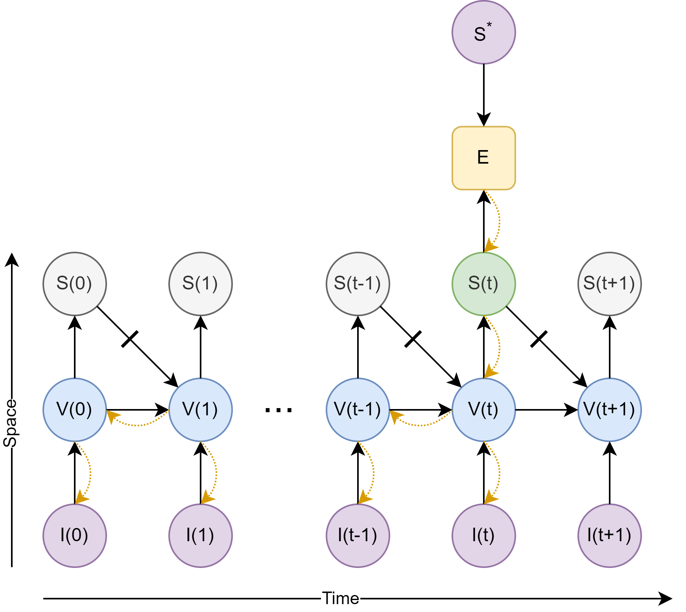
Figure 1: Computational graph for a 5 time steps simulation on a 1-layer SNN using soft-reset LIF neurons and back-propagation through time. Where I, V and S are vectors representing the neuron input, voltage and output spike, respectively. $\text{S}^{*}$ is the target output and E is the error. The black arrows represent the forward pass of the data, while the curved orange arrows represent the gradient backward pass. The neuron resets is detached from the computational graph in the gradient calculation.

$$\begin{split}\frac{dE}{dW}={}&\frac{\partial E}{\partial V(t)}\frac{\partial V(t)}{\partial W}+\frac{\partial E}{\partial V(t-1)}\frac{\partial V(t-1)}{\partial W}+\ldots+\\ &+\frac{\partial E}{\partial V(0)}\frac{\partial V(0)}{\partial W}\end{split}$$ (3a)

$$\begin{split}\frac{dE}{dW}={}&\frac{\partial E}{\partial V(t)}I(t)+\frac{\partial E}{\partial V(t-1)}I(t-1)+\ldots+\\ &+\frac{\partial E}{\partial V(0)}I(0)\end{split}$$ (3b)

In classification problems, the cross-entropy loss function is often used. However, as this depends on the softmax activation function which is not local (it depends on all output neurons values for the final calculation), we have used the Mean Squared Error (MSE). Consequently, the gradient of the error with respect to the network weights (according to equation 1) would be as on equation 3b

Following equation 1, the gradients of the network are as follows:

$$\frac{\partial S(t)}{\partial V(t)}=\phi(V(t)-A(t))=\varphi(t)\leavevmode\nobreak\ \frac{\partial V(t)}{\partial V(t-1)}=\alpha$$ (4)

$$\frac{\partial E}{\partial S(t)}=S(t)-S^{*}\leavevmode\nobreak\ \frac{\partial V(t)}{\partial W}=I(t)$$

where $\phi(x)$ is the surrogate gradient of the Heaviside function (H), $S^{*}$ the target output, $S(t)$ the output spike of the neuron and I(t) the input at time $t$.

Assuming that the error is calculated at time t=T and calling $\frac{dE(t)}{dV(t)}=(S(t)-S^{*})$, the gradient of the error with respect to the weights in a period of time T is defined as an equation of three factors (equation 2d) which we will call: (1) pre-synaptic spike trace (blue), (2) surrogate gradient of the post-synaptic voltage (green) and (3) external signal (red). The pre-synaptic spike trace can be expressed as a low-pass filter of the input spikes to the neuron at each synapse, derived from equation 2c as formulated in equation 5.

$$\varepsilon_{pre}(t)=\alpha\varepsilon_{pre}(t-1)+I(t)$$ (5)

Since the threshold adaptation must be taken into account for the gradient computation of the ALIF model, the product of (1) the pre-synaptic spike trace and (2) the surrogate gradient of the post-synaptic voltage is modified according to equation 6 [3], where $e(t)$ is a function of (1) the pre-synaptic spike trace $\varepsilon(t)$, (2) the surrogate gradient of the post-synaptic voltage $\psi$ and (3) the threshold adaptation trace $a(t)$ at time step $t$, $\theta$ is the increase in the adaptive threshold, and $\gamma$ is the threshold decay constant.

$$\varepsilon_{adapt}(t) =\varepsilon_{pre}(t)\varphi(t)+(\gamma-\varphi(t)\theta)\varepsilon_{adapt}(t-1)$$ (6)

$$e(t) =\varphi(t)(\varepsilon_{pre}(t)-\theta\varepsilon_{adapt}(t))$$ (7)

II-C Spatial dependency

The back-propagation of the errors in calculating the network gradients means that there is a spatial dependency in training. This dependency results in non-local update to each neuron or synapse for two main reasons: (1) weight update locking and (2) weight transport problem as explained in section I).

DRTP solves this problem by using one-hot-encoded targets in supervised classification problems as a proxy for the sign of the error [18]. Therefore, instead of waiting for the data to propagate forward through the layers to calculate the global error which would be then back-propagated, the targets (i.e. labels) are used directly. Together with feedback alignment using fixed random weights from the teaching neurons in the gradient computation, DRTP solves both spatial dependency problems (i.e. update locking and weight transport) [18]. Since there is no propagation of gradient information between layers, the gradient computation is performed in a similar way in each layer, so the computational graph (Fig. 1) is the same across layers. The difference is that, instead of using the gradient of the error, the projected labels are used. As a result, in contrast with eProp, there is no need for a synaptic eligibility trace which we define as a low-pass filter of the Hebbian component (i.e. pre- and pos-synaptic information) of the learning rule [20].

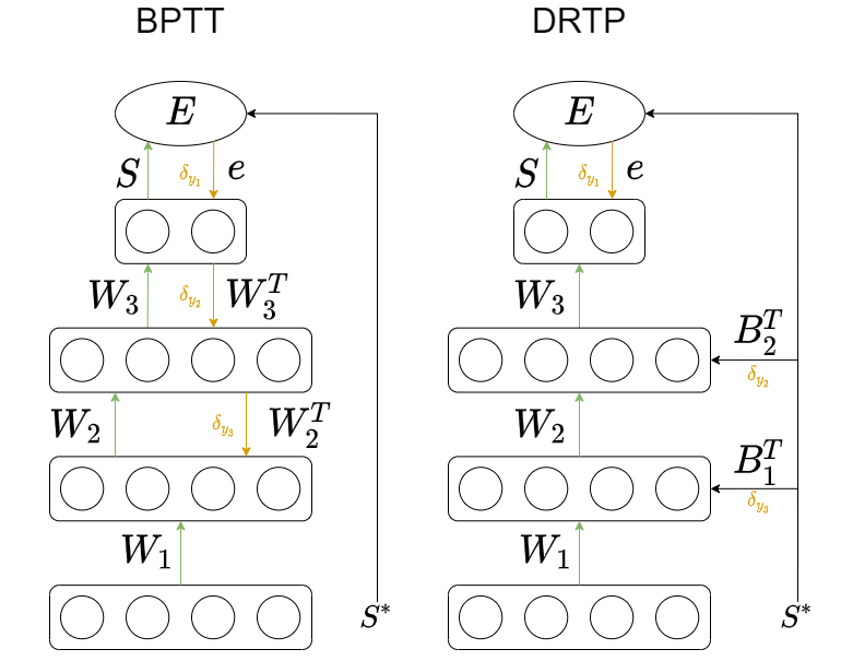
Figure 2: Weight update mechanism on BPTT and DRTP. In the case of BPTT, and error is calculated using the output layer and the target $S^{*}$, the error is then propagated backward through the layers using the transpose of the synaptic weights. On DRTP, the error is only calculated at the output layer, the weights in the hidden layer are updated using directly the target, using random fixed matrix.

II-D ETLP

ETLP is based on a many-to-one learning architecture [54], where the error is calculated at a specific time step of an input streaming data (Fig. 1), that can be defined as a random point in an input sequence of spikes, as defined in section II-B. Learning is made using target labels with one-hot-encoding, representing the targets as teaching neurons. Since the targets are represented as a one-hot-encoded vector, and the learning algorithm is updated using a many-to-one architecture (as exposed in section II-B), they can be represented as teaching neurons that fire an event at the end of a time window. The teaching neurons have synapses that connect them to the output neurons and the neurons in the hidden layers, firing at a certain frequency (e.g. $100\ Hz$), obtaining a fully event-based supervised learning technique.

II-D1 Synapse traces

In the case of an ALIF neuron, each synapse requires two traces: (1) the pre-synaptic spike trace (equation 8) which holds the pre-synaptic activity information, where $I(t)$ represent the input spike and $\alpha$ the neuron time constant, and (2) the threshold adaptation trace (equation 10) which holds the threshold value depending on the post-synaptic activity. In the case of a LIF, only a trace of the pre-synaptic spikes are required. Finally, $e(t)$ in equation 11 consists of a combination of the pre-synaptic spike trace, the surrogate gradient of the post-synaptic voltage (equation 9) and the threshold adaptation trace when using the ALIF neuron.

$$\varepsilon_{pre}(t) =\alpha\varepsilon_{pre}(t-1)+I(t)$$ (8)

$$\varphi(t) =\gamma max\left(0,1-\left|V(t)-A(t)\right|\right)$$ (9)

$$\varepsilon_{adapt}(t) =\varepsilon_{pre}(t)\varphi(t)+(\gamma-\varphi(t)\theta)\varepsilon_{adapt}(t-1)$$ (10)

$$e(t) =\varphi(t)(\varepsilon_{pre}(t)-\theta\varepsilon_{adapt}(t))$$ (11)

The update of synapses is event-driven, i.e., each time the postsynaptic (hidden or output) neuron receives an input spike from a master neuron. In the case of hidden layers, the update is performed based on the equation 12, where $I$ represents the input from the teaching neurons and $e$ the product of surrogate gradient and pre-synaptic and threshold adaptation traces. Thus, by using only local information per synapse (pre-synaptic and post-synaptic values), as well as a firing signal from a neuron, learning only takes place when an activation signal is received from the learning neurons.

II-D2 Synaptic plasticity

The synapse update is event-driven, i.e., each time the post-synaptic neuron (hidden or output) receives a spike from a teaching neuron. In the case of the hidden layers, the update is made based on equation 12, where $I$ represent the input from the teaching neurons. Thus, ETLP learning uses local information per synapse (pre-synaptic spike trace, surrogate gradient of the post-synaptic voltage and teaching neurons weights) and is triggered when a spike from a teaching neuron is received. Otherwise, the weights of the network are not updated. For the output layer, two different types of connections are made between the teaching neurons and the output layer. Each teaching neuron is connected in a one-to-one fashion with an excitatory synapse with the output neurons and with the other output neurons with an inhibitory synapse. As a result, the output neuron receive an input current $I$ that each time it receive an input spike from the teaching neuron, applying equation 13, where $e_{out}$ is the function over the pre-synaptic spike trace, the surrogate gradient of the post-synaptic voltage and the threshold adaptation trace of the output neuron, and $s_{out}$ is the spike of the output neuron.

$$W(t+1)_{in/rec}=W(t)_{in/rec}+\gamma I(t)e(t)_{in/rec}\\$$ (12)

$$W(t+1)_{out}=W(t)_{out}+\gamma\frac{2s(t)_{out}-I(t)-1}{2}e(t)_{out}$$ (13)

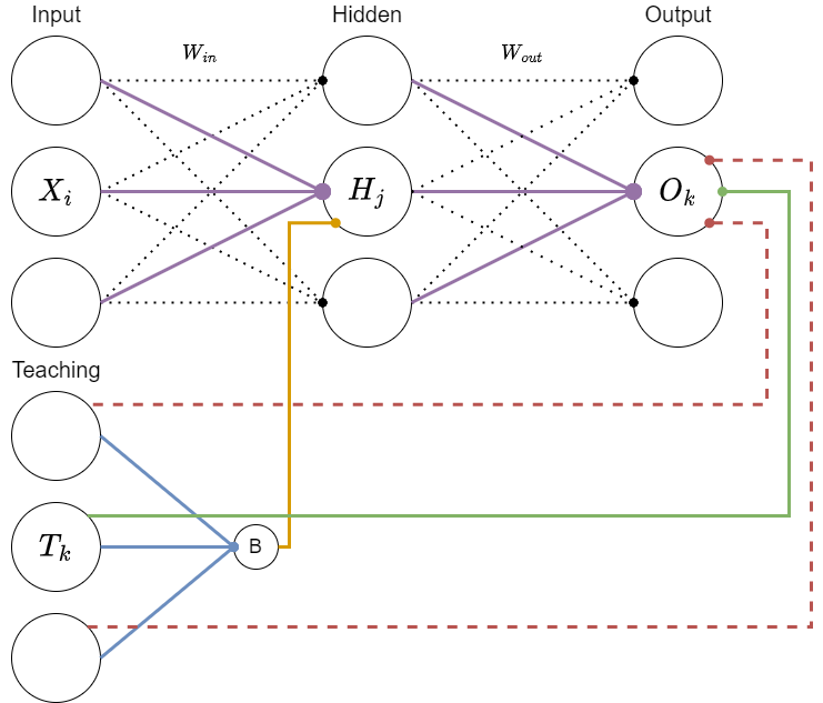
Figure 3: Feedforward SNN with ETLP learning. The network consists of a hidden layer, an output layer and teaching neurons. The output layer is connected to the teaching neurons by both excitatory (green) and inhibitory (dashed red) synapses. The learning layer is also connected to the group of recurrent neurons via a random weight matrix B. When a class is active, the neuron in the learning layer starts to emit spikes at a certain frequency (e.g. 100Hz), thus modifying the synapses of the neurons according to the equations 12 and 13.

III Results

To test the performance of ETLP, the rule was compared with BPTT (non-local in time and space) and eProp (non-local in space) on two different datasets. The final accuracy calculation is based on a rate decoding (i.e. winning neuron is the one firing most during the sample presentation) of the final layer’s output spikes.

The first dataset is Neuromorphic-MNIST (N-MNIST) [40], recorded by moving the ATIS sensor over MNIST samples (10 classes) in three saccades of 100ms each. The resulting information is therefore mainly spatial, where the temporal structure is exclusively related to the movements of the sensor. The second dataset is Spiking Heidelberg Digits (SHD) [10], a set of 10000 spoken digit audios from 0 to 9 in both English and German (20 classes). The dataset was generated using an artificial cochlea, producing spikes in 700 input channels. In contrast with N-MNIST, SHD contains both a spatial and a rich temporal structure [42].

For N-MNIST, we used only the first saccade of about 100ms with a time step of of 1ms, resulting in 100 time steps per sample. For SHD, we limited the samples duration to 1s with a time step of 10ms to result in 100 time steps per sample, similar to N-MNIST. This time binning provides enough temporal information to reach a state-of-the-art performance in accuracy [5].

The hyper-parameters used on the simulations for both datasets are shown in Tab. I, where dt is the algorithmic timestep, lr the learning rate, $\tau_{m}$ the membrane decay time constant, $\tau_{a}$ the threshold adaptation decay time constant, $v_{th}$ the base threshold. The PyTorch software implementation is publicly available on Github . All the results presented in this section are averaged over three runs with different random initialization of the synaptic weights.

Table I: Hyperparameter used on SHD and N-MNIST datasets.

Parameter	N-MNIST	SHD
dt	1ms	10ms
lr	$5e^{-4}$	$5e^{-4}$
$\tau_{m}$	80ms	1000ms
$\tau_{a}$	10ms	1000ms
$v_{th}$	1	1
batch size	128	128
Hidden size	200	450
Refactory period (time steps)	5	5

III-A N-MNIST

For the N-MNIST dataset, a feedforward network of LIF neurons with 2064 input neurons ($32\times 32=1032$ neurons for each polarity), 200 hidden neurons and 10 output neurons was used. Indeed, explicit recurrence is not needed when the information in the data are mostly spatial [5].

The results on N-MNIST dataset are shown in Figs. 4 and 4a, for training and test set respectively. ETLP shows an accuracy of 94.30% on the test set, compared to 97.90% and 97.67% for eProp and BPTT respectively. BPTT results are on par with the state-of-the-art with a similar topology [42, 5], while eProp reaches a lightly higher accuracy which is probably due to hyper-parameters. On the other hand, ETLP loses 3.60% compared to eProp.

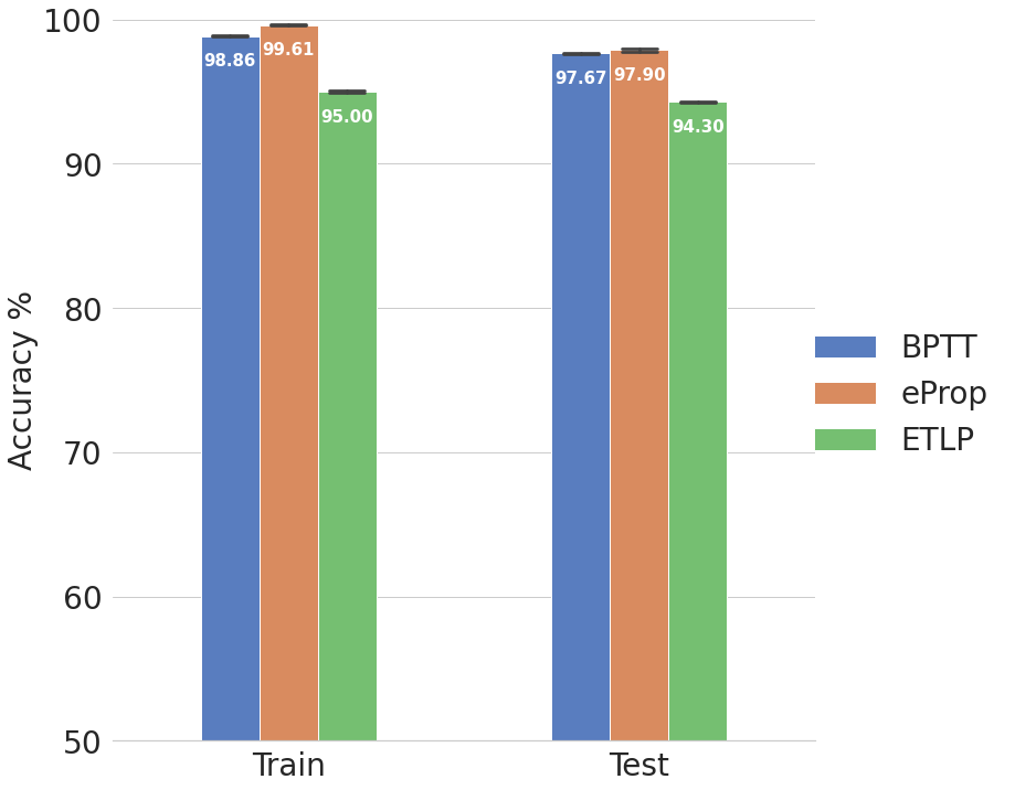
(a)

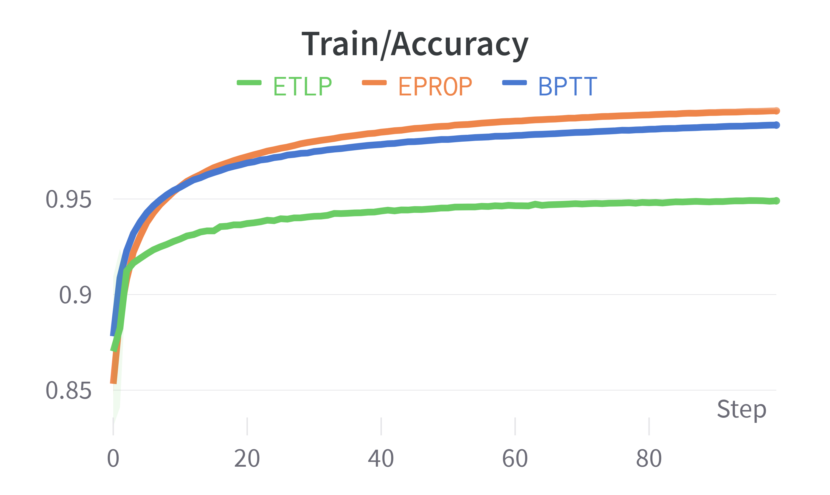
(b)

(c)

Figure 4: Accuracy of BPTT, eProp and ETLP on N-MNIST using a feedforward network of LIF neurons. Fig. (a) shows a comparison in accuracy between the training and test datasets, Figs. (b) and (c) show the accuracy over all the epochs for training and test, respectively.

III-B SHD

For the SHD dataset, since it has more temporal dependency than N-MNIST [42], we tested both feedforward and recurrent networks with all-to-all explicit recurrent connections in the hidden layer. Both networks used 700 input neurons, 450 hidden neurons and 20 output neurons. Two different neuron models were explored: LIF and ALIF.

For the feedforward topology, a LIF model was used. ETLP has an accuracy of 59.19%, compared to 66.33% and 63.04% for BPTT and eProp respectively, as shown in Fig. 6.

For the recurrent topology, an initial exploration over the $\theta$ parameter of the adaptive threshold has been made. Several simulations have been performed for each rule and for each $\theta$ parameter (0, 5 and 10) to see how it affects the accuracy. Tab. II shows the accuracy for each learning rule and $\theta$ parameter, where the $\theta$ value used for the final results is marked in green.

In the case of ETLP, a higher maximum accuracy is obtained with $\theta=5$. However, it can be seen in Fig. 5 that this accuracy then decreases with the epochs, going below the accuracy with $\theta=10$. Hence, $\theta=10$ is taken as the best value because it is more important to have a convergence with more data than to reach a maximum accuracy at a particular epoch.

Table II: Test accuracy of $\theta$ parameter exploration on BPTT, eProp and ETLP. On SHD dataset with a RSNN.

Learning	$\theta=0$		$\theta=5$		$\theta=10$
Method	$\mu$	$\sigma$	$\mu$	$\sigma$	$\mu$	$\sigma$
BPTT	75.23	0.44	64.43	0.68	23.96	0.67
eProp	51.68	1.10	80.79	0.39	49.94	1.98
ETLP	48.53	0.64	78.71	1.49	74.59	0.44

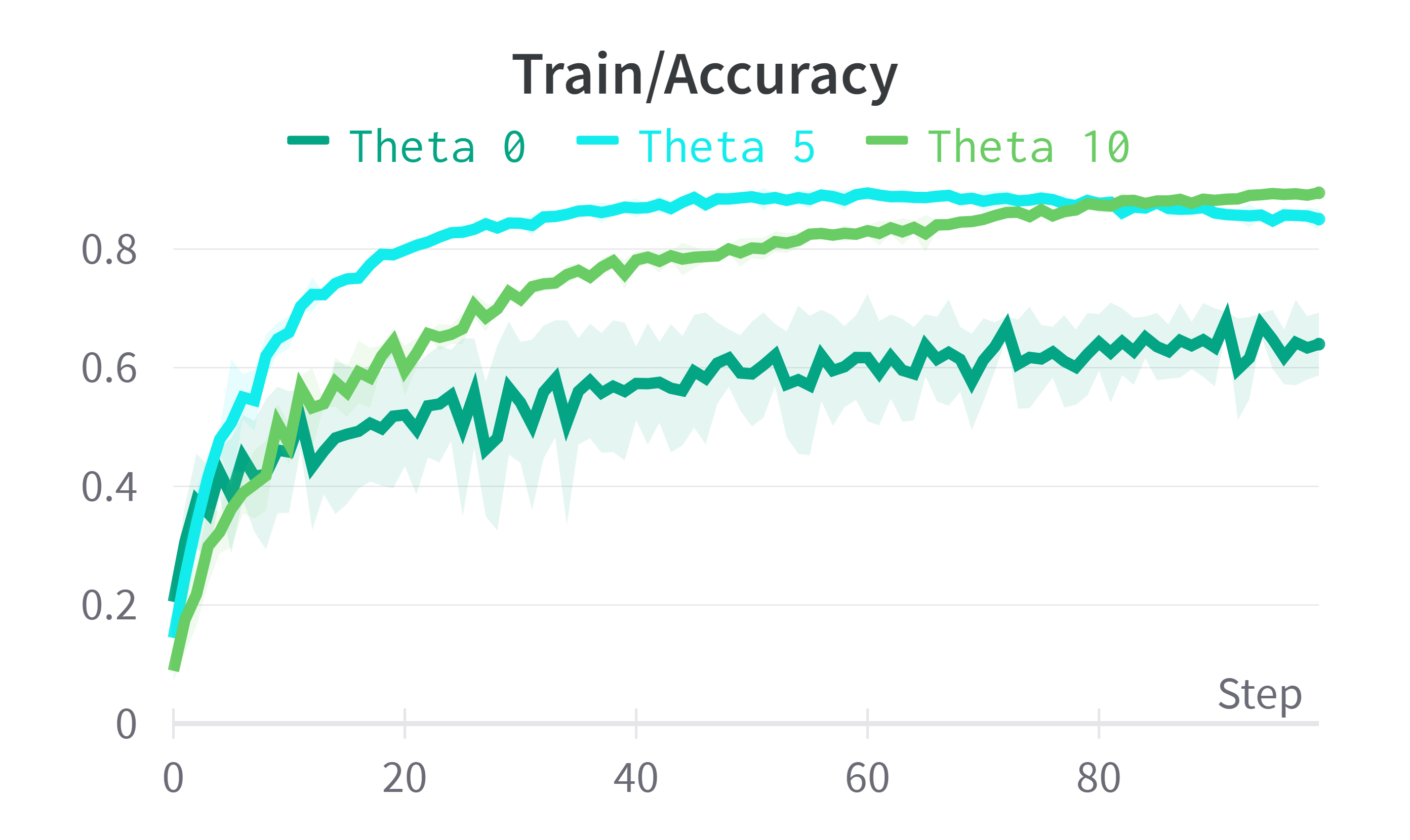
(a)

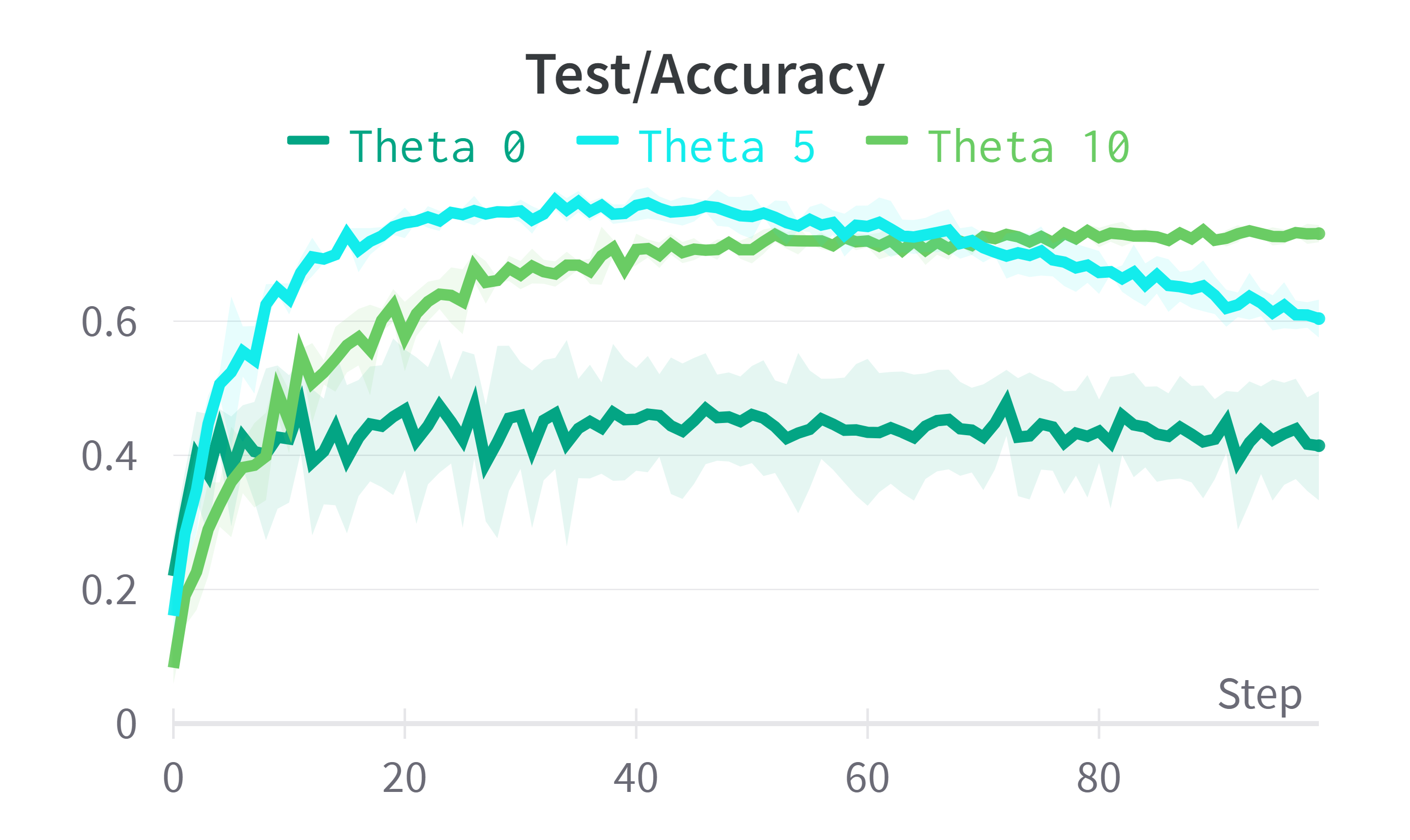
(b)

Figure 5: Accuracy for different threshold adaptation on ETLP in SHD dataset with the recurrent network.

The final results obtained on SHD dataset using a recurrent topology are shown in Fig. 6 based on the best $\theta$ parameter obtained per learning rule. ETLP ($\theta=10$) achieves a test accuracy of 74.59%, showing a slight loss compared to BPTT ($\theta=0$) that reaches 75.23% and a consequent loss of 6.20% compared to eProp that reaches 80.79%. We observe that adding explicit recurrence in the hidden layer of the network increases accuracy by a considerable amount of 8.90% for BPTT, 17.75% for eProp and 15.40% for ETLP. We also observe that the the BPTT offline learning reaches a better accuracy without threshold adaptation (i.e. $\theta=0$), while it is required for the online learning of eProp (although spatially non-local) and ETLP.

It is to note that, similar to [42], we did not reach the state-of-the-art accuracy with BPTT that reaches 80.41% with a similar topology [5]. This can be explained by the different training strategies where the output layer in [5] is not spiking, as well as the chosen hyper-parameters that were not tuned specifically for BPTT. Hence, BPTT reaches in principle a better accuracy than both eProp and ETLP.

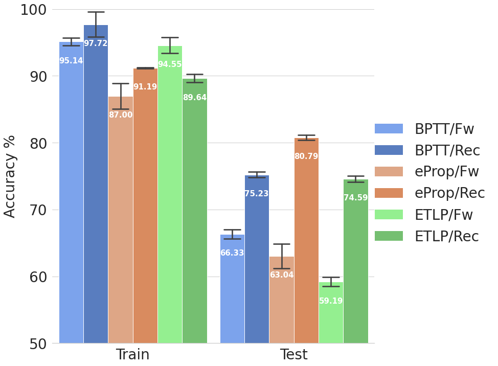
(a)

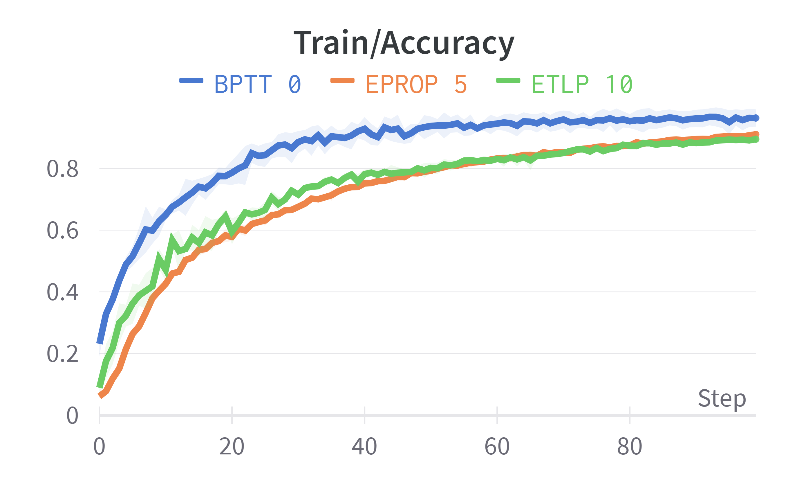
(b)

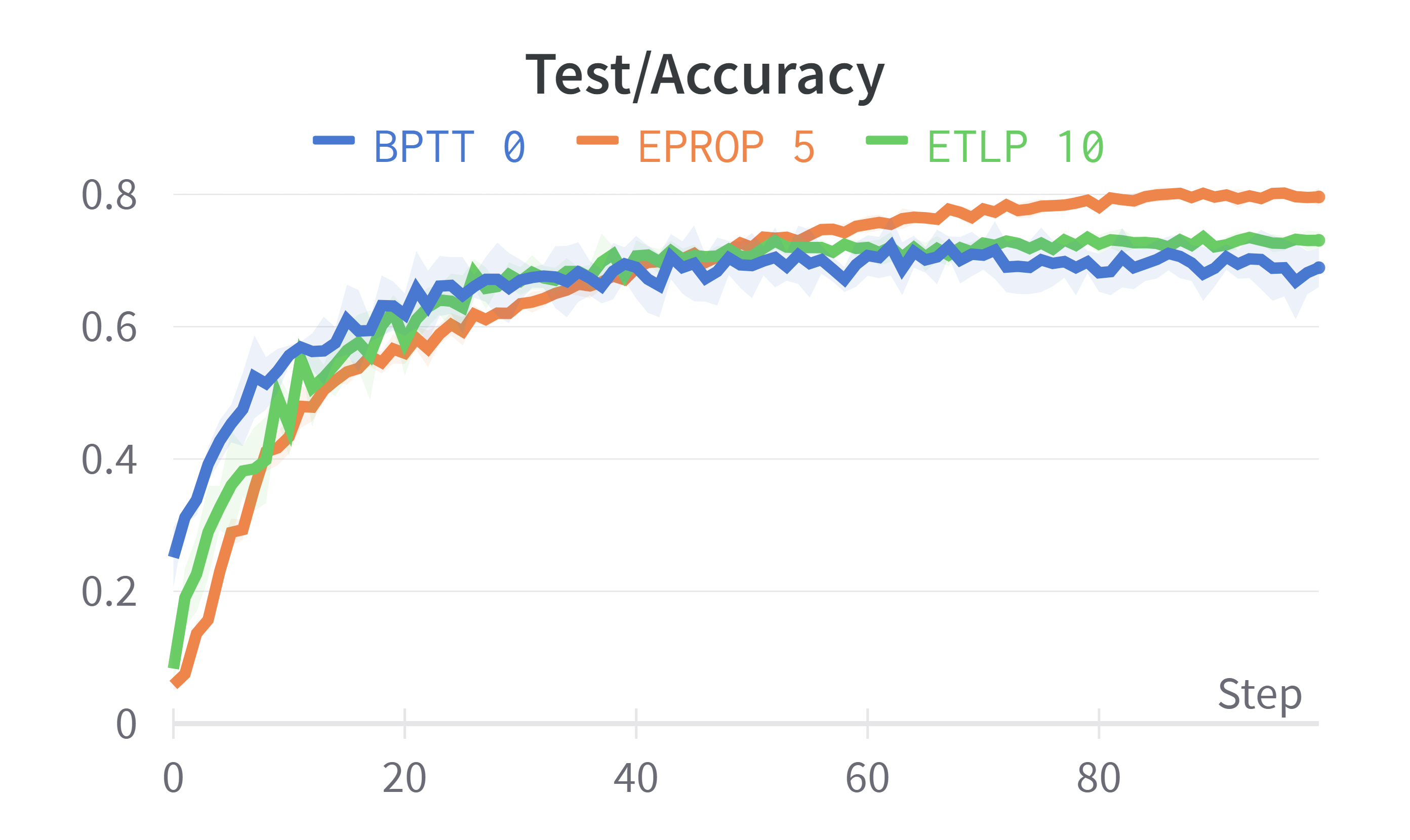
(c)

Figure 6: Accuracy of BPTT, eProp and ETLP on SHD. Fig. (a) shows a comparison in accuracy between the feedforward network with LIF neurons and the recurrent network with ALIF neurons. Figs. (b) and (c) show the accuracy of the the recurrent network for each learning rule on the training and test datasets, respectively, with the best $\theta$ value obtained for each one.

IV Hardware implementation

ETLP could be easily implemented on a neuromorphic hardware, resulting in a low-latency and low-power consumption alternative for online learning. As a proof of concept, a Field-Programmable Gate Array (FPGA) implementation of the ETLP module for calculating the weight update based on [44] has been designed, as shown in Fig. 7. The module receives the following signals as input for the gradient calculation:

1. The address of the pre-synaptic neuron that is connected to the synapse to be updated;

2. The output of the pre-synaptic neuron (0 or 1) for the pre-synaptic spike trace calculation;

3. The voltage value of the post-synaptic neuron for the surrogate voltage calculation;

4. The teaching value, equal to the teaching neurons weights when they emit a spike which triggers the weight update.

The implemented surrogate gradient shown in Fig. 8) is the triangular function, defined as $f(x)=max(0,1-|x|)$.

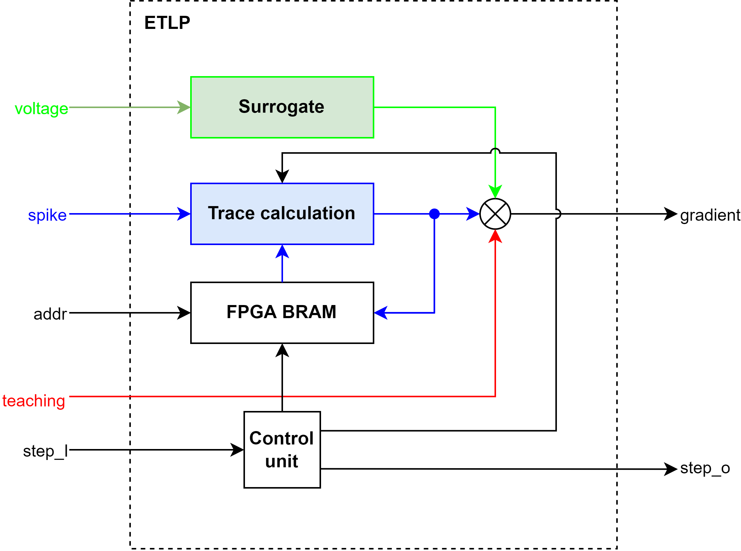
Figure 7: FPGA implementation for ETLP module. The control unit triggers the calculation of the new pre-synaptic spike trace value and stores it in memory. Once the gradient is calculated, it sends the control signal to the upper module so that it can read the calculated gradient value.

Figure 8: Triangular function surrogate gradient implementation on FPGA.

Figure 9: pre-synaptic spike trace calculation on FPGA. In the case of a pre-synaptic spike arrives, a constant is added to the new pre-synaptic spike trace value.

We assume to use some time-multiplexing handled by the upper module, but do not go into its architectural details as the ETLP implementation is independent. The ETLP module stores pre-synaptic spike trace values in a BRAM. Each time a step signal is received, the module retrieves the stored trace, calculates the new trace value and stores it back into memory. At the same time, it calculates the surrogate gradient from the value of the post-synaptic voltage. When both results are obtained, the final gradient is calculated with their product with the signal coming from the teaching neuron. Finally, the module produces a step signal to indicate to the upper module that it can update the corresponding synaptic weight. This module can be optimized for asynchronous updates of the gradient (i.e. only when a spike from the teaching neurons is received).

This module takes three clock cycles to perform the calculation. Fig. 10 shows a time diagram of the process. The module would be in the “initial” state until a signal from $step\_I$ is received. Then, it gathers the pre-synaptic spike trace from memory (“read” state), calculates the gradient value, and write the new pre-synaptic spike trace into memory (“write” state). Finally it produces an output signal to notify the upper module that the gradient value is available and changes the state back to “init”.

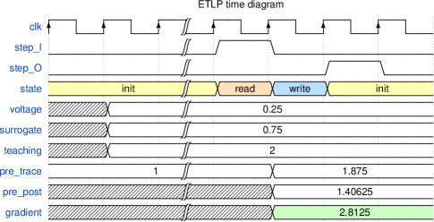
Figure 10: ETLP FPGA implementation time diagram.

The module has been synthesised on a Nexys4 DDR (xc7a100tcsg324-1) FPGA with the resource consumption shown in Tab. III. A power estimation has been carried out at different clock frequencies. With a 100MHz clock, the device static and dynamic power consumption are approximately 97mW and 53mW respectively, where 47mW corresponds to I/O. With a 10MHz clock, the static power consumption is the same while the dynamic power consumption is reduced to 5mW, where 4.5mW corresponds to I/O. Finally, with a 1MHz clock, the dynamic power consumption is negligible, since the value is smaller than the resolution provided by the tool (below 1mW).

Interestingly, when using one module per neuron, a 1MHz clock is sufficient to update a neuron in the hidden layer of our recurrent SNN with SHD, since the number of required clock cycles per second is (700 [synapses from input layer neurons] + 450 [synapses from hidden layer neurons) * 100 [updates per second] * 3 [clock cycles per updates] = 345,000, meaning a clock frequency of 345KHz. We can therefore expect a low-power consumption for the full network, especially when designing an Application-Specific Integrated Circuit (ASIC) with a similar architecture.

Table III: Resource utilization of ETLP module

Resource	Used	Available	Util%
Slice LUTs	115	63400	0.18
Flip Flop	22	126800	0.02%
DSPs	2	240	0.83%
BRAM tile	1	270	0.37%

V Discussion and conclusion

In this work, we have proposed the ETLP rule, a local learning rule in time and space which is triggered asynchronously based on the availability of the target or label. These features satisfy the hardware constraints of neuromorphic chips where computing and memory are co-localized. We compared ETLP to eProp (non-local in space) and BPTT (non-local in time and space), and achieved a test accuracy of 94.30% on N-MNIST with a feedforward network of LIF neurons and 74.59% on SHD with a recurrent network of ALIF neurons. ETLP has a loss of accuracy of 3.60% and 6.20% compared to the best accuracy of eProp on N-MNIST and SHD, respectively, which is reasonable due to its fully event-driven and local plasticity paradigm.

Two features have a major impact on the accuracy when learning SHD spatio-temporal patterns that have a rich temporal structure. First, adding an all-to-all explicit recurrence in the hidden layer reduces training over-fitting and highly increases test accuracy by 8.90%, 17.75% and 15.40% for BPTT, eProp and ETLP, respectively. This confirms the results reported on BPTT in [5]. Second, the threshold adaptation of the ALIF improves the accuracy of ETLP and eProp by 26.06% and 29.11%, respectively, while it decreases the accuracy of BPTT by 10.80%. Although we did not extensively explore the reasons behind this behavior, it is clear for ETLP that the threshold adaptation provides an online dynamic mechanism (in addition to the refractory period) to limit the neurons firing rate. In BPTT, it might not be needed since the error signal is explicitly back-propagated and used in the weight updates. An additional mechanism to explore for ETLP to further reduce the firing rate and potentially gain energy-efficiency is the voltage regularization based on additional plasticity mechanisms such as the homeostatic membrane potential dependent synaptic plasticity [1].

Table IV: Complexity analysis of the gradient computation over different learning rules. N represents the number of input neurons; M the number of neurons in a layer; T the length of the back-propagated sequence; Nr the number of readout neurons in DECOLLE; p the ratio of connected neurons/total possible.

Learning	Space	Time
BPTT	$O(NT)$	$O(pNMT)$
e-Prop	$O(pNM)$	$O(pNM)$
DECOLLE [24]	$O(1)$	$O(MNr+pNM)$
ETLP	$O(1)$	$O(pNM)$

In addition to the accuracy benchmarking, we demonstrated a proof of concept hardware implementation on FPGA to show how it is possible to map the local computational primitives of ETLP on digital neuromorphic chips. It is also a way to better understand the simplicity of the plasticity mechanism in hardware, where the required information are two Hebbian pre-synaptic (spike trace) and post-synaptic (voltage put in a simple function) factors [25] and a third factor in the form of an external signal provided by the target or label. Therefore, ETLP is compatible with neuromorphic chips such as Loihi2 which supports on-chip three-factor local plasticity [12, 39]. Table IV shows a comparison of the computational complexity of BPTT, eProp, DECOLLE [24] and ETLP. We can see that ETLP is indeed local in space like DECOLLE (ETLP uses DRTP while DECOLLE uses local losses) and local in time like eProp (although ETLP needs one spike trace per pre-synaptic neuron only, while eProp needs in addition an eligibility trace per synapse), thus being more computationally efficient than previously proposed plasticity mechanisms.

ETLP builds on previous developments toward more local learning mechanisms, and proposes a fully-local synaptic plasticity model that fits with the hardware constraints of neuromorphic chips for online learning with low-energy consumption and real-time interaction. We have shown a good classification accuracy on visual and auditory benchmarks, both starting from a randomly initialized network to show a proof of convergence. Future works will focus on implementing ETLP on a more realistic experimental setup with few-shot learning. In order to adapt to new classes that have not been seen before, new labels will be provided to the network to automatically trigger plasticity. The open question is how to design the output layer, either by having more neurons that needed at the beginning or by adding new neurons when needed. Since few-shot learning is based on very few labeled samples, we can train both initial network synaptic weights and ETLP hyper-parameters based on the Model-Agnostic Meta-Learning (MAML) that has been recently applied to SNNs [48].

Fernando M. Quintana received the B.S. degree in Computer Engineering from the University of Cadiz (Spain), where he also obtained the master’s degree in Computer and Systems Engineering Research. He is currently pursuing his Ph.D. degree on local and online learning in Spiking Neural Networks.

Fernando Perez-Peña received the Engineering degree in Telecommunications from the University of Seville (Spain) and his Ph.D. degree (specialized in neuromorphic motor control) from the University of Cadiz (Cadiz, Spain) in 2009 and 2014 respectively. In 2015 he was a postdoc at CITEC (Bielefeld University, Germany). He has been an Assistant Professor in the Architecture and Technology of Computers Department of the University of Cadiz since 2014. His research interests include neuromorphic engineering, CPG, motor control and neurorobotics.

Pedro L. Galindo is Professor of Computer Science and Engineering and leader of the Intelligent Systems group at the University of Cadiz, Spain. His main research interest is the the application of Artificial Intelligence to the solution of real-world problems in industrial environments, especially those arised in Industry 4.0.

Emre O. Neftci received his MSc degree in physics from EPFL in Switzerland, and his Ph.D. in 2010 at the Institute of Neuroinformatics at the University of Zurich and ETH Zurich. He is currently an institute director at the Jülich Research Centre and Professor at RWTH Aachen. His current research explores the bridges between neuroscience and machine learning, with a focus on the theoretical and computational modeling of learning algorithms that are best suited to neuromorphic hardware and non-von Neumann computing architectures.

Elisabetta Chicca received a “Laurea” degree (M.Sc.) in Physics from the University of Rome 1 “La Sapienza”, Italy in 1999 with a thesis on CMOS spike-based learning. In 2006 she received a Ph.D. in Natural Science from the Swiss Federal Institute of Technology Zurich (ETHZ, Physics department) and in Neuroscience from the Neuroscience Center Zurich. E. Chicca has carried out her research as a Postdoctoral fellow (2006-2010) and as a Group Leader (2010-2011) at the Institute of Neuroinformatics (University of Zurich and ETH Zurich) working on development of neuromorphic signal processing and sensory systems. From 2011 to 2020 she lead the Neuromorphic Behaving Systems (NBS) research group at Bielefeld University (Faculty of Technology and Cognitive Interaction Technology Center of Excellence, CITEC). She is currently the Chair of the Bioinspired Circuits and Systems (BICS) Laboratory, Faculty of Science and Engineering, University of Groningen, Groningen, The Netherlands. She has a long-standing experience with developing event-based neuromorphic systems and their application to biologically inspired computational models. Her research activities cover models of cortical circuits for brain-inspired computation, learning in spiking neural networks, bio-inspired sensing, and motor control.

Lyes Khacef received his MSc in embedded systems from the University of Nice Sophia Antipolis (France). He pursued a PhD at Université Cote d’Azur (France) in brain-inspired computing where he worked on self-organizing neuromorphic architectures on FPGA for multimodal unsupervised learning based on local structural and synaptic plasticity. He then started a Postdoc at the University of Groningen (the Netherlands) where he is working on the modeling and hardware prototyping of spike-based local synaptic plasticity mechanisms for online learning of spatio-temporal patterns at the edge.

References

- [1] C. Albers, M. Westkott, and K. .Pawelzik, “Learning of precise spike times with homeostatic membrane potential dependent synaptic plasticity,” PLOS ONE, vol. 11, no. 2, pp. 1–28, 02 2016.
- [2] A. Basu, L. Deng, C. Frenkel, and X. Zhang, “Spiking neural network integrated circuits: A review of trends and future directions,” in 2022 IEEE Custom Integrated Circuits Conference (CICC), 2022, pp. 1–8.
- [3] G. Bellec, F. Scherr, A. Subramoney, E. Hajek, D. Salaj, R. Legenstein, and W. Maass, “A solution to the learning dilemma for recurrent networks of spiking neurons,” Nature Communications, vol. 11, no. 1, p. 3625, July 2020.
- [4] Y. Bengio, D. H. Lee, J. Bornschein, and Z. Lin, “Towards biologically plausible deep learning,” ArXiv, vol. abs/1502.04156, 2015.
- [5] M. S. Bouanane, D. Cherifi, E. Chicca, and L. Khacef, “Impact of spiking neurons leakages and network recurrences on event-based spatio-temporal pattern recognition,” 2022. [Online]. Available: https://arxiv.org/abs/2211.07761
- [6] I. Boybat, M. Gallo, N. S.R., T. Moraitis, T. Parnell, T. Tuma, B. Rajendran, Y. Leblebici, A. Sebastian, and E. Eleftheriou, “Neuromorphic computing with multi-memristive synapses,” Nature Communications, vol. 9, June 2018.
- [7] E. Ceolini, C. Frenkel, S. B. Shrestha, G. Taverni, L. Khacef, M. Payvand, and E. Donati, “Hand-gesture recognition based on emg and event-based camera sensor fusion: A benchmark in neuromorphic computing,” Frontiers in Neuroscience, vol. 14, p. 637, 2020. [Online]. Available: https://www.frontiersin.org/article/10.3389/fnins.2020.00637
- [8] E. Chicca, F. Stefanini, C. Bartolozzi, and G. Indiveri, “Neuromorphic electronic circuits for building autonomous cognitive systems,” Proceedings of the IEEE, vol. 102, no. 9, pp. 1367–1388, 2014.
- [9] D. V. Christensen, R. Dittmann, B. Linares-Barranco, A. Sebastian, M. L. Gallo, A. Redaelli, S. Slesazeck, T. Mikolajick, S. Spiga, S. Menzel, I. Valov, G. Milano, C. Ricciardi, S.-J. Liang, F. Miao, M. Lanza, T. J. Quill, S. T. Keene, A. Salleo, J. Grollier, D. Marković, A. Mizrahi, P. Yao, J. J. Yang, G. Indiveri, J. P. Strachan, S. Datta, E. Vianello, A. Valentian, J. Feldmann, X. Li, W. H. P. Pernice, H. Bhaskaran, S. Furber, E. Neftci, F. Scherr, W. Maass, S. Ramaswamy, J. Tapson, P. Panda, Y. Kim, G. Tanaka, S. Thorpe, C. Bartolozzi, T. A. Cleland, C. Posch, S. Liu, G. Panuccio, M. Mahmud, A. N. Mazumder, M. Hosseini, T. Mohsenin, E. Donati, S. Tolu, R. Galeazzi, M. E. Christensen, S. Holm, D. Ielmini, and N. Pryds, “2022 roadmap on neuromorphic computing and engineering,” Neuromorphic Computing and Engineering, vol. 2, no. 2, p. 022501, May 2022. [Online]. Available: https://dx.doi.org/10.1088/2634-4386/ac4a83
- [10] B. Cramer, Y. Stradmann, J. Schemmel, and F. Zenke, “The heidelberg spiking data sets for the systematic evaluation of spiking neural networks,” IEEE Transactions on Neural Networks and Learning Systems, 2020.
- [11] W. M. Czarnecki, G. Swirszcz, M. Jaderberg, S. Osindero, o. Vinyals, and K. Kavukcuoglu, “Understanding synthetic gradients and decoupled neural interfaces,” in Proceedings of the 34th International Conference on Machine Learning - Volume 70, ser. ICML’17. JMLR.org, 2017, p. 904–912.
- [12] M. Davies, N. Srinivasa, T.-H. Lin, G. Chinya, Y. Cao, S. H. Choday, G. Dimou, P. Joshi, N. Imam, S. Jain, Y. Liao, C.-K. Lin, A. Lines, R. Liu, D. Mathaikutty, S. McCoy, A. Paul, J. Tse, G. Venkataramanan, Y.-H. Weng, A. Wild, Y. Yang, and H. Wang, “Loihi: A neuromorphic manycore processor with on-chip learning,” IEEE Micro, vol. 38, no. 1, pp. 82–99, 2018.
- [13] M. Davies, A. Wild, G. Orchard, Y. Sandamirskaya, G. A. F. Guerra, P. Joshi, P. Plank, and S. R. Risbud, “Advancing neuromorphic computing with loihi: A survey of results and outlook,” Proceedings of the IEEE, vol. 109, no. 5, pp. 911–934, 2021.
- [14] R. H. DENNARD, F. H. GAENSSLEN, H.-N. YU, V. LEO RIDEOVT, E. BASSOUS, and A. R. LEBLANC, “Design of ion-implanted mosfet’s with very small physical dimensions,” IEEE Solid-State Circuits Society Newsletter, vol. 12, no. 1, pp. 38–50, 2007.
- [15] R. H. Dennard, V. Rideout, E. Bassous, and A. LeBlanc, “Design of ion-implanted mosfet’s with very small physical dimensions,” Solid-State Circuits, IEEE Journal of, vol. 9, no. 5, pp. 256–268, 1974.
- [16] J. K. Eshraghian, M. Ward, E. Neftci, X. Wang, G. Lenz, G. Dwivedi, M. Bennamoun, D. S. Jeong, and W. D. Lu, “Training spiking neural networks using lessons from deep learning,” 2021.
- [17] C. Frenkel, D. Bol, and G. Indiveri, “Bottom-up and top-down neural processing systems design: Neuromorphic intelligence as the convergence of natural and artificial intelligence,” 2021.
- [18] C. Frenkel, M. Lefebvre, and D. Bol, “Learning without feedback: Fixed random learning signals allow for feedforward training of deep neural networks,” Frontiers in Neuroscience, vol. 15, p. 20, Feb. 2021. [Online]. Available: https://www.frontiersin.org/article/10.3389/fnins.2021.629892
- [19] C. Frenkel, M. Lefebvre, J.-D. Legat, and D. Bol, “A 0.086-mm2 12.7-pj/sop 64k-synapse 256-neuron online-learning digital spiking neuromorphic processor in 28-nm cmos,” IEEE Transactions on Biomedical Circuits and Systems, vol. 13, no. 1, pp. 145–158, 2019.
- [20] W. Gerstner, M. Lehmann, V. Liakoni, D. Corneil, and J. Brea, “Eligibility traces and plasticity on behavioral time scales: Experimental support of neohebbian three-factor learning rules,” Frontiers in Neural Circuits, vol. 12, p. 53, 2018.
- [21] W. Gerstner, R. Ritz, and J. L. van Hemmen, “Why spikes? hebbian learning and retrieval of time-resolved excitation patterns,” Biological cybernetics, vol. 69, no. 5-6, p. 503—515, 1993.
- [22] G. Indiveri, B. Linares-Barranco, T. Hamilton, A. van Schaik, R. Etienne-Cummings, T. Delbruck, S. Liu, P. Dudek, P. Häfliger, S. Renaud, J. Schemmel, G. Cauwenberghs, J. Arthur, K. Hynna, F. Folowosele, S. Saighi, T. Serrano-Gotarredona, J. Wijekoon, Y. Wang, and K. Boahen, “Neuromorphic silicon neuron circuits,” Frontiers in Neuroscience, vol. 5, pp. 1–23, 2011.
- [23] E. Izhikevich, “Solving the distal reward problem through linkage of STDP and dopamine signaling,” Cereb. Cortex, Jan. 2007, in press.
- [24] J. Kaiser, H. Mostafa, and E. Neftci, “Synaptic plasticity dynamics for deep continuous local learning (decolle),” Frontiers in Neuroscience, vol. 14, p. 424, 2020.
- [25] L. Khacef, P. Klein, M. Cartiglia, A. Rubino, G. Indiveri, and E. Chicca, “Spike-based local synaptic plasticity: A survey of computational models and neuromorphic circuits,” 2022. [Online]. Available: https://arxiv.org/abs/2209.15536
- [26] Y. LeCun, L. Bottou, Y. Bengio, and P. Haffner, “Gradient-based learning applied to document recognition,” Proceedings of the IEEE, vol. 86, no. 11, pp. 2278–2324, 1998.
- [27] Y. LeCun et al., “Deep learning,” Nature, vol. 521, no. 7553, pp. 436–444, 2015.
- [28] T. P. Lillicrap, D. Cownden, D. B. Tweed, and C. Akerman, “Random synaptic feedback weights support error backpropagation for deep learning,” Nature Communications, vol. 7, no. 13276, pp. 1–10, 2016.
- [29] H. Markram, P. J. Helm, and B. Sakmann, “Dendritic calcium transients evoked by single back-propagating action potentials in rat neocortical pyramidal neurons,” The Journal of physiology, vol. 485 ( Pt 1), p. 1—20, May 1995.
- [30] B. L. McNaughton, R. M. Douglas, and G. V. Goddard, “Synaptic enhancement in fascia dentata: Cooperativity among coactive afferents,” Brain Research, vol. 157, no. 2, pp. 277–293, 1978.
- [31] C. Mead and L. Conway, Introduction to VLSI Systems. Reading, Massachusetts: Addison-Wesley, 1980.
- [32] A. Morrison, M. Diesmann, and W. Gerstner, “Phenomenological models of synaptic plasticity based on spike timing,” Biological Cybernetics, vol. 98, pp. 459–478, 2008.
- [33] H. Mostafa, V. Ramesh, and G. Cauwenberghs, “Deep supervised learning using local errors,” Frontiers in Neuroscience, vol. 12, p. 608, 2018.
- [34] A. R. Muliukov, L. Rodriguez, B. Miramond, L. Khacef, J. Schmidt, Q. Berthet, and A. Upegui, “A unified software/hardware scalable architecture for brain-inspired computing based on self-organizing neural models,” Frontiers in Neuroscience, vol. 16, 2022. [Online]. Available: https://www.frontiersin.org/articles/10.3389/fnins.2022.825879
- [35] S. F. Muller-Cleve, V. Fra, L. Khacef, A. Pequeno-Zurro, D. Klepatsch, E. Forno, D. G. Ivanovich, S. Rastogi, G. Urgese, F. Zenke, and C. Bartolozzi, “Braille letter reading: A benchmark for spatio-temporal pattern recognition on neuromorphic hardware,” 2022. [Online]. Available: https://arxiv.org/abs/2205.15864
- [36] E. O. Neftci, C. Augustine, S. Paul, and G. Detorakis, “Event-driven random back-propagation: Enabling neuromorphic deep learning machines,” Frontiers in Neuroscience, vol. 11, p. 324, 2017.
- [37] E. O. Neftci, H. Mostafa, and F. Zenke, “Surrogate gradient learning in spiking neural networks: Bringing the power of gradient-based optimization to spiking neural networks,” IEEE Signal Processing Magazine, vol. 36, no. 6, pp. 51–63, 2019.
- [38] A. Nøkland, “Direct feedback alignment provides learning in deep neural networks,” in Advances in Neural Information Processing Systems, D. Lee, M. Sugiyama, U. Luxburg, I. Guyon, and R. Garnett, Eds., vol. 29. Curran Associates, Inc., 2016.
- [39] G. Orchard, E. P. Frady, D. B. D. Rubin, S. Sanborn, S. B. Shrestha, F. T. Sommer, and M. Davies, “Efficient neuromorphic signal processing with loihi 2,” CoRR, vol. abs/2111.03746, 2021. [Online]. Available: https://arxiv.org/abs/2111.03746
- [40] G. Orchard, A. Jayawant, G. K. Cohen, and N. Thakor, “Converting static image datasets to spiking neuromorphic datasets using saccades,” Frontiers in neuroscience, vol. 9, p. 437, 2015.
- [41] M. Payvand, F. Moro, K. Nomura, T. Dalgaty, E. Vianello, Y. Nishi, and G. Indiveri, “Self-organization of an inhomogeneous memristive hardware for sequence learning,” Nature Communications, vol. 13, p. 5793, Oct. 2022.
- [42] N. Perez-Nieves, V. Leung, P. Dragotti, and D. Goodman, “Neural heterogeneity promotes robust learning,” Nature Communications, Oct. 2021.
- [43] N. Qiao, H. Mostafa, F. Corradi, M. Osswald, F. Stefanini, D. Sumislawska, and G. Indiveri, “A re-configurable on-line learning spiking neuromorphic processor comprising 256 neurons and 128k synapses,” Frontiers in Neuroscience, vol. 9, no. 141, 2015.
- [44] F. M. Quintana, F. Perez-Peña, and P. L. Galindo, “Bio-plausible digital implementation of a reward modulated stdp synapse,” Neural Computing and Applications, vol. 34, pp. 15 649–15 660, 9 2022. [Online]. Available: https://link.springer.com/article/10.1007/s00521-022-07220-6
- [45] J. M. Rabaey, M. Verhelst, J. D. Boeck, C. Enz, K. D. Greve, A. M. Ionescu, M. Na, K. P. (editors) with F. Conti, F. Corradi, K. D. Greve, M. D. Ketelaere, B. Dhoedt, M. Hartmann, K. Myny, I. Ocket, W. Philips, W. Verachtert, and D. Verkest, “Ai at the edge - a roadmap,” Technical report by IMEC, KU Leuven, Ghent University, VUB, EPFL, ETH Zurich and UC Berkeley, 2019.
- [46] C. D. Schuman, T. E. Potok, R. M. Patton, J. D. Birdwell, M. E. Dean, G. S. Rose, and J. S. Plank, “A Survey of Neuromorphic Computing and Neural Networks in Hardware,” arXiv, pp. 1–88, 2017.
- [47] J. Shalf, “The future of computing beyond moore’s law,” Philosophical Transactions of the Royal Society A: Mathematical, Physical and Engineering Sciences, vol. 378, no. 2166, p. 20190061, 2020. [Online]. Available: https://royalsocietypublishing.org/doi/abs/10.1098/rsta.2019.0061
- [48] K. Stewart and E. Neftci, “Meta-learning spiking neural networks with surrogate gradient descent,” CoRR, vol. abs/2201.10777, 2022. [Online]. Available: https://arxiv.org/abs/2201.10777
- [49] G. Stuart and B. Sakmann, “Active propagation of somatic action potentials into neocortical pyramidal cell dendrites,” Nature, vol. 367, no. 69-72, 1994.
- [50] J. Stuijt, M. Sifalakis, A. Yousefzadeh, and F. Corradi, “brain: An event-driven and fully synthesizable architecture for spiking neural networks,” Frontiers in Neuroscience, vol. 15, 2021. [Online]. Available: https://www.frontiersin.org/articles/10.3389/fnins.2021.664208
- [51] N. C. Thompson, K. Greenewald, K. Lee, and G. F. Manso, “Deep learning’s diminishing returns: The cost of improvement is becoming unsustainable,” IEEE Spectrum, vol. 58, no. 10, pp. 50–55, 2021.
- [52] N. C. Thompson, K. H. Greenewald, K. Lee, and G. F. Manso, “The computational limits of deep learning,” CoRR, vol. abs/2007.05558, 2020. [Online]. Available: https://arxiv.org/abs/2007.05558
- [53] F. Zenke and S. Ganguli, “Superspike: Supervised learning in multilayer spiking neural networks,” Neural Computation, vol. 30, no. 6, pp. 1514–1541, June 2018.
- [54] F. Zenke and E. O. Neftci, “Brain-inspired learning on neuromorphic substrates,” Proceedings of the IEEE, vol. 109, no. 5, pp. 935–950, 2021.