KdV breathers on a cnoidal wave background

Abstract.

Using the Darboux transformation for the Korteweg-de Vries equation, we construct and analyze exact solutions describing the interaction of a solitary wave and a traveling cnoidal wave. Due to their unsteady, wavepacket-like character, these wave patterns are referred to as breathers. Both elevation (bright) and depression (dark) breather solutions are obtained. The nonlinear dispersion relations demonstrate that the bright (dark) breathers propagate faster (slower) than the background cnoidal wave. Two-soliton solutions are obtained in the limit of degeneration of the cnoidal wave. In the small amplitude regime, the dark breathers are accurately approximated by dark soliton solutions of the nonlinear Schrödinger equation. These results provide insight into recent experiments on soliton-dispersive shock wave interactions and soliton gases.

1. Introduction

The localized and periodic traveling wave solutions of the Korteweg-de Vries (KdV) equation are so ubiquitous and fundamental to nonlinear science that their names, “soliton” and “cnoidal wave,” have achieved a much broader usage, representing localized and periodically extended traveling wave solutions across a wide range of nonlinear evolutionary equations. Consequently, it is natural and important to consider their interactions. While the traditional notion of linear superposition cannot be used, the complete integrability of the KdV equation implies a nonlinear superposition principle. For example, soliton interactions can be described by exact $N$-soliton solutions, which can be constructed by successive Darboux transformations [1]. By utilizing solutions of the spectral problem for the stationary Schrödinger equation and the temporal evolution equation whose compatibility is equivalent to solving the KdV equation, the Darboux transformation achieves a nonlinear superposition principle by effectively “adding” one soliton to the base solution. In the spectral problem, the soliton appears as an additional eigenvalue that is added to the spectrum of the base solution.

Compared to soliton interactions, soliton-cnoidal wave interactions have not been explored in as much detail. The purpose of this paper is to apply the Darboux transformation to the cnoidal wave solution of the KdV equation in order to obtain the nonlinear superposition of a single soliton and a cnoidal wave. These exact solutions, expressed in terms of Jacobi theta functions and elliptic integrals, represent the interactions of a soliton and a cnoidal wave.

The motivation for this study comes from recent experiments and analysis of the interaction of solitons and dispersive shock waves (DSWs) [2, 3, 4]. The DSWs can be viewed as modulated cnoidal waves [5, 6] so that soliton-DSW interaction is analogous to soliton-cnoidal wave interaction. Two different types of soliton-DSW interaction dynamics were observed in [2]. When a soliton completely passes through a DSW, the nature of the interaction gives rise to an elevation (bright) nonlinear wavepacket. When a soliton becomes embedded or trapped within a DSW, the trapped soliton resembles a depression (dark) nonlinear wavepacket. Similar transmission and trapping scenarios were analyzed for solitons interacting with rarefaction waves [7, 8].

Breathers are localized, unsteady solutions that exhibit two distinct time scales or velocities; one associated with propagation and the other with internal oscillations. A canonical model equation that admits breather solutions is the focusing modified Korteweg-de Vries (mKdV) equation. These solutions can be interpreted as bound states of two soliton solutions [9, 10]. It is in a similar spirit that we regard as a breather, the soliton-cnoidal wave interactions considered here. Such wavepacket solutions are propagating, nonlinear solutions with internal oscillations.

Among our main results, we find two distinct varieties of exact solutions of the KdV equation, corresponding to elevation (bright) or depression (dark) breathers interacting with the cnoidal wave background. These breathers are topological because they impart a phase shift to the cnoidal wave. We show that bright breathers propagate faster than the cnoidal wave, whereas dark breathers move slower. Furthermore, bright breathers of sufficiently small amplitude exhibit a negative phase shift, whereas bright breathers of sufficiently large amplitude exhibit a positive phase shift. On the other hand, dark breathers with the strongest localization have a positive phase shift. Small amplitude dark breathers can exhibit either a negative or positive phase shift. Each breather solution is characterized by its position and a spectral parameter, determining a nonlinear dispersion relation, which uniquely relates the breather velocity to the breather phase shift.

Exact solutions representing soliton-cnoidal wave interactions have previously been constructed using other solution methods. The first result was developed in [11] within the context of the stability analysis of a cnoidal wave of the KdV equation. The authors used the Marchenko equation of the inverse scattering transform and obtained exact solutions for “dislocations” of the cnoidal wave. More special solutions for soliton-cnoidal wave interactions were obtained in [12] by using the nonlocal symmetries of the KdV equation. These solutions are expressed in a closed form as integrals of Jacobi elliptic functions, but they do not represent the most general exact solutions for soliton-cnoidal wave interactions.

Quasi-periodic (finite-gap) solutions and solitons on a quasi-periodic background have been obtained as exact solutions of the KdV equation by using algebro-geometric methods [13, 14]. In the limit of a single gap, such solutions describe interactions of solitons with a cnoidal wave. By using the degeneration of hyperelliptic curves and Sato Grassmannian theory, mixing between solitons and quasi-periodic solutions was obtained recently in [15] based on [16], not only for the KdV equation but also for the KP hierarchy of integrable equations. Finally, in a very recent preprint [17], inspired by recent works on soliton gases [18, 19], the degeneration of quasi-periodic solutions was used to construct multisoliton-cnoidal wave interaction solutions.

Compared to previous work, which primarily involve Weierstrass functions with complex translation parameters, we give explicit solutions in terms of Jacobi elliptic functions with real-valued parameters. This approach allows us to clarify the nature of soliton-cnoidal wave interactions, plot their corresponding properties, and analyze the exact solutions in various limiting regimes. We also demonstrate that the Darboux transformation provides a more straightforward method for obtaining these complicated interaction solutions compared to the degeneration methods used in [15, 17].

The paper is organized as follows. The main results are formulated in Section 2 and illustrated graphically. In Section 3, we introduce the normalized cnoidal wave solution with one parameter. Symmetries of the KdV equation are then introduced that can be used to generate the more general family of cnoidal waves with four arbitrary parameters. Eigenfunctions of the stationary Schrödinger equation with the normalized cnoidal wave potential are reviewed in Section 4. The time evolution of the eigenfunctions is obtained in Section 5. In Section 6, the Darboux transformation is used to generate breather solutions to the KdV equation. Properties of bright and dark breathers are explored in Sections 7 and 8, respectively. The paper concludes with Section 9.

2. Main results

We take the Korteweg–de Vries (KdV) equation in the normalized form

$$u_{t}+6uu_{x}+u_{xxx}=0,$$ (1)

where $t$ is the evolution time, $x$ is the spatial coordinate for wave propagation, and $u$ is the fluid velocity. As is well-known [20], every smooth solution $u(x,t)$ of the KdV equation (1) is the compatibility condition of the stationary Schrödinger equation

$$(-\partial_{x}^{2}-u)v=\lambda v$$ (2)

and the time evolution problem

$$v_{t}=(4\lambda-2u)v_{x}+u_{x}v,$$ (3)

where $\lambda$ is the $(x,t)$-independent spectral parameter.

The normalized traveling cnoidal wave of the KdV equation (1) is given by

$$u(x,t)=\phi_{0}(x-c_{0}t),\qquad\phi_{0}(x):=2k^{2}{\rm cn}^{2}(x,k),\quad c_{0}:=4(2k^{2}-1),$$ (4)

where ${\rm cn}(x,k)$ is the Jacobi elliptic function, and $k\in(0,1)$ is the elliptic modulus. Table 1 collects together elliptic integrals and Jacobi elliptic functions used in our work, see [21, 22, 23].

The main result of this work is the derivation and analysis of two solution families of the KdV equation (1) parametrized by $\lambda$ and $x_{0}\in\mathbb{R}$, where $\lambda$ belongs to $(-\infty,-k^{2})$ for the first family and $(1-2k^{2},1-k^{2})$ for the second family. Both the solution families can be expressed in the form

$$u(x,t)=2\left[k^{2}-1+\frac{E(k)}{K(k)}\right]+2\partial_{x}^{2}\log\tau(x,t),$$ (5)

where the $\tau$-function for the first family is given by

$$\tau(x,t):=\Theta(x-c_{0}t+\alpha_{b})e^{\kappa_{b}(x-c_{b}t+x_{0})}+\Theta(x-c_{0}t-\alpha_{b})e^{-\kappa_{b}(x-c_{b}t+x_{0})}$$ (6)

with uniquely defined $\kappa_{b}>0$, $c_{b}>c_{0}$ and $\alpha_{b}\in(0,K(k))$ and the $\tau$-function for the second family is given by

$$\tau(x,t):=\Theta(x-c_{0}t+\alpha_{d})e^{-\kappa_{d}(x-c_{d}t+x_{0})}+\Theta(x-c_{0}t-\alpha_{d})e^{\kappa_{d}(x-c_{d}t+x_{0})}$$ (7)

with uniquely defined $\kappa_{d}>0$, $c_{d}<c_{0}$, and $\alpha_{d}\in(0,K(k))$.

Figure 1 depicts the spatiotemporal evolution of a solution $u(x,t)$ given by (5) and (6). This solution represents a bright breather on a cnoidal wave background (hereafter referred to as a bright breather) with speed $c_{b}>c_{0}$ and inverse width $\kappa_{b}$, where $c_{0}$ is the speed of the background cnoidal wave. As a result of the bright soliton, the cnoidal wave background is spatially shifted by $-2\alpha_{b}$.

Figure 1. Bright breather on a cnoidal wave with $k=0.8$ for $\lambda=-1.2$ and $x_{0}=0$.

Figure 2. Dark breather on a cnoidal wave with $k=0.7$ for $\lambda=0.265$ and $x_{0}=0$.

Figure 2 shows the spatiotemporal evolution of a solution $u(x,t)$ given by (5) and (7). This solution is a dark breather on a cnoidal wave background (hereafter referred to as a dark breather), where the breather core exhibits the inverse spatial width $\kappa_{d}$ and speed $c_{d}<c_{0}$. The dark breather gives rise to the spatial shift $2\alpha_{d}$ of the cnoidal background.

Using properties of Jacobi elliptic functions, we obtain explicit expressions for the parameters of the $\tau$-functions (6) and (7) and their dependence on the parameter $\lambda$ that characterizes the dynamical properties of bright and dark breathers. Although the analytical expressions (5) with either (6) or (7) are not novel and can be found in equivalent forms in [11, 15, 17], it is the first time to the best of our knowledge that the dynamical properties of bright and dark breathers have been explicitly investigated for the KdV equation (1). We also obtain asymptotic expressions for bright and dark breathers in the limits when $\lambda$ approaches the band edges or when the elliptic modulus $k$ approaches the end points $0$ and $1$.

3. Traveling cnoidal wave

A traveling wave solution $u(x,t)=\phi(x-ct)$ to the KdV equation (1) satisfies the second-order differential equation after integration in $x$:

$$\phi^{\prime\prime}+3\phi^{2}-c\phi=b,$$ (8)

where $b\in\mathbb{R}$ is the integration constant and the single variable $x$ stands for $x-ct$. The second-order equation (8) is integrable with the first-order invariant

$$(\phi^{\prime})^{2}+2\phi^{3}-c\phi^{2}-2b\phi=d,$$ (9)

where $d\in\mathbb{R}$ is another integration constant. The following proposition summarizes the existence of periodic solutions to system (8) and (9).

Proposition 1.

There exists a family of periodic solutions to system (8) and (9) for every $(b,c,d)$ satisfying $c^{2}+12b>0$ and $d\in(U(\phi_{+}),U(\phi_{-}))$, where $U(\phi):=2\phi^{3}-c\phi^{2}-2b\phi$ and $\phi_{\pm}$ are critical points of $U$ given by $\phi_{\pm}=(c\pm\sqrt{c^{2}+12b})/6$.

Proof.

If $c^{2}+12b>0$, the mapping $\phi\mapsto U(\phi)$ has two critical points $\phi_{\pm}$. Since $U^{\prime}(\phi_{\pm})=6\phi_{\pm}^{2}-2c\phi_{\pm}-2b=0$ and $U^{\prime\prime}(\phi_{\pm})=12\phi_{\pm}-2c=\pm 2\sqrt{c^{2}+12b}$, $\phi_{+}$ is the minimum of $U$ and $\phi_{-}$ is the maximum of $U$. If $d=U(\phi_{+})$, the only bounded solution of system (8) and (9) is a constant solution corresponding to the center point $(\phi_{+},0)$. If $d=U(\phi_{-})$, the only bounded solution of system (8) and (9) is a homoclinic orbit from the saddle point $(\phi_{-},0)$ which surrounds the center point $(\phi_{+},0)$. The family of periodic orbits exists in a punctured neighbourhood around the center point enclosed by the homoclinic orbit, for $d\in(U(\phi_{+}),U(\phi_{-}))$.

If $c^{2}+12b\leq 0$, the mapping $\phi\mapsto U(\phi)$ is monotonically increasing. There exist no bounded solutions of system (8) and (9) with the exception of the constant solution $\phi=c/6$ in the marginal case $c^{2}+12b=0$. ∎

It follows from Proposition 1 that the most general periodic traveling wave solution has three parameters $(b,c,d)$, up to translations, that are defined in a subset of $\mathbb{R}^{3}$ for which $c^{2}+12b>0$ and $d\in(U(\phi_{+}),U(\phi_{-}))$. For each $(b,c,d)$ in this subset of $\mathbb{R}^{3}$, the translational parameter $x_{0}\in\mathbb{R}$ generates the family of solutions $\phi(x+x_{0})$ due to translation symmetry.

Two of the three parameters of the periodic solution family can be chosen arbitrarily due to the following two symmetries of the KdV equation (1):

• Scaling transformation: if $u(x,t)$ is a solution, so is $\alpha^{2}u(\alpha x,\alpha^{3}t)$, $\alpha>0$.

• Galilean transformation: if $u(x,t)$ is a solution, so is $\beta+u(x-6\beta t,t)$, $\beta\in\mathbb{R}$.

Due to these symmetries, if $\phi_{0}$ is a periodic solution to system (8) and (9) with $(b,c,d)=(b_{0},c_{0},d_{0})$, then $\beta+\alpha^{2}\phi_{0}(\alpha x)$ is also a periodic solution to system (8) and (9) with

$$(b,c,d)=(-3\beta^{2}-\alpha^{2}\beta c_{0}+\alpha^{4}b_{0},6\beta+\alpha^{2}c_{0},2\beta^{3}+\alpha^{2}\beta^{2}c_{0}-2\beta\alpha^{4}b_{0}+\alpha^{6}d_{0}),$$

where $\alpha>0$ and $\beta\in\mathbb{R}$ are arbitrary parameters. Thus, without loss of generality, we can consider the normalized, 1-parameter family of periodic traveling waves $\phi_{0}(x)=2k^{2}{\rm cn}^{2}(x,k)$ for which the values of $(b_{0},c_{0},d_{0})$ are determined in the following proposition.

Proposition 2.

The normalized cnoidal wave $\phi_{0}(x)=2k^{2}{\rm cn}^{2}(x,k)$ is a periodic solution of system (8) and (9) with

$$b_{0}:=4k^{2}(1-k^{2}),\quad c_{0}:=4(2k^{2}-1),\quad d_{0}=0,$$

where $k\in(0,1)$ is an arbitrary parameter.

Proof.

Since $\min\limits_{x\in\mathbb{R}}\phi_{0}(x)=0$, it follows from (9) that $d_{0}=U(0)=0$. On the other hand, by using the following fundamental relations between Jacobi elliptic functions

$${\rm sn}^{2}(x,k)+{\rm cn}^{2}(x,k)=1,\quad{\rm dn}^{2}(x,k)+k^{2}{\rm sn}^{2}(x,k)=1$$ (10)

and their derivatives

$$\frac{d}{dx}\left[\begin{array}[]{l}{\rm sn}(x,k)\\ {\rm cn}(x,k)\\ {\rm dn}(x,k)\end{array}\right]=\left[\begin{array}[]{l}{\rm cn}(x,k){\rm dn}(x,k)\\ -{\rm sn}(x,k){\rm dn}(x,k)\\ -k^{2}{\rm sn}(x,k){\rm cn}(x,k)\end{array}\right],$$ (11)

we obtain from (9) with $d_{0}=0$ that $b_{0}=4k^{2}(1-k^{2})$ and $c_{0}=4(2k^{2}-1)$. ∎

4. Lamé equation as the spectral problem

The spectral problem (2) with the normalized cnoidal wave (4) is known as the Lamé equation [24, p.395]. It can be written in the form

$$v^{\prime\prime}(x)-2k^{2}{\rm sn}^{2}(x,k)v(x)+\eta v(x)=0,\quad\eta:=\lambda+2k^{2},$$ (12)

where the single variable $x$ stands for $x-c_{0}t$. By using (10) and (11), we obtain the following three particular solutions $v=v_{1,2,3}(x)$ of the Lamé equation (12) with $\lambda=\lambda_{1,2,3}(k)$:

$$\lambda_{1}(k):=-k^{2},\qquad v_{1}(x):={\rm dn}(x,k),$$

$$\lambda_{2}(k):=1-2k^{2},\qquad v_{2}(x):={\rm cn}(x,k),$$

$$\lambda_{3}(k):=1-k^{2},\qquad v_{3}(x):={\rm sn}(x,k),$$

which correspond to the three remarkable values of $\eta$: $\eta_{1}=k^{2}$, $\eta_{2}=1$, and $\eta_{3}=1+k^{2}$. For $k\in(0,1)$, the three eigenvalues are sorted as $\lambda_{1}(k)<\lambda_{2}(k)<\lambda_{3}(k)$.

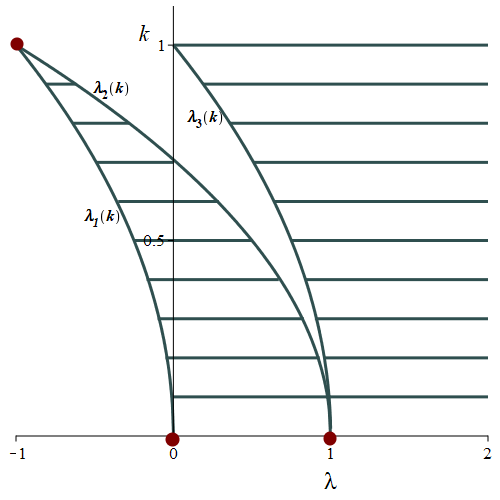
Figure 3. Floquet spectrum of the Lamé equation (12) for different values of $k\in(0,1)$.

Figure 3 shows the Floquet spectrum of the Lamé equation (12), which corresponds to the admissible values of $\lambda$ for which $v\in L^{\infty}(\mathbb{R})$. The bands are shaded and the band edges shown by the bold solid curves corresponding to $\lambda=\lambda_{1,2,3}(k)$ for $k\in(0,1)$. The cnoidal wave is the periodic potential with a single finite gap (the so-called one-zone potential) [25] so that the Floquet spectrum consists of the single finite band $[\lambda_{1}(k),\lambda_{2}(k)]$ and the semi-infinite band $[\lambda_{3}(k),\infty)$.

As is well-known (see [24, p. 395]), the two linearly independent solutions of the Lamé equation (12) for $\lambda\neq\lambda_{1,2,3}(k)$ are given by the functions

$$v_{\pm}(x)=\frac{H(x\pm\alpha)}{\Theta(x)}e^{\mp xZ(\alpha)},$$ (13)

where $\alpha\in\mathbb{C}$ is found from $\lambda\in\mathbb{R}$ by using the characteristic equation $\eta=k^{2}+{\rm dn}^{2}(\alpha,k)$ and the Jacobi zeta function is $Z(\alpha):=\frac{\Theta^{\prime}(\alpha)}{\Theta(\alpha)}=Z(\varphi_{\alpha},k)$ with $\varphi_{\alpha}=\mathrm{am}(\alpha,k)$ [21, 144.01], see Table 1. Since $\eta=\lambda+2k^{2}$, the characteristic equation can be written in the form

$$\lambda=1-2k^{2}+k^{2}{\rm cn}^{2}(\alpha,k).$$ (14)

The following proposition clarifies how $\alpha$ is defined from the characteristic equation (14) when $\lambda$ is decreased from $\lambda_{3}(k)$ to $-\infty$. Figure 4 illustrates the path of $\alpha$ in the complex plane.

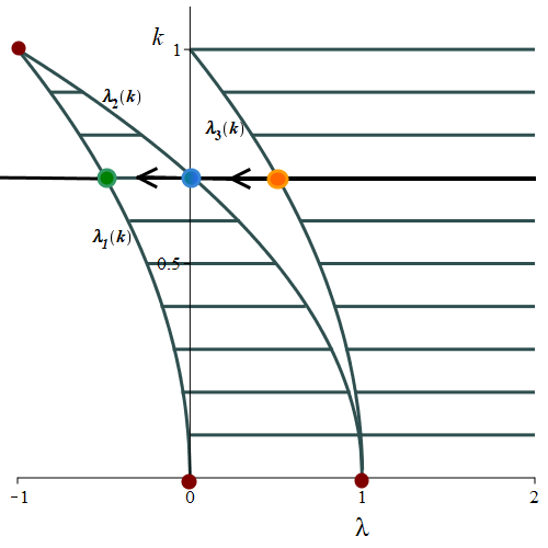
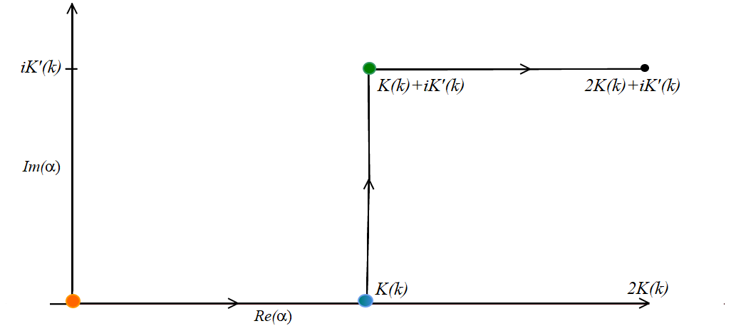
Figure 4. Left: Floquet spectrum with orange, blue, and green dots corresponding to $\lambda_{3}(k)$, $\lambda_{2}(k)$, and $\lambda_{1}(k)$, respectively, for a fixed value of $k\in(0,1)$. Right: The complex plane for the parameter $\alpha$ indicating the path of $\alpha$ corresponding to the path of $\lambda$ in (14).

Proposition 3.

Fix $k\in(0,1)$. We have

• $\alpha=F(\varphi_{\alpha},k)\in[0,K(k)]$ for $\lambda\in[\lambda_{2}(k),\lambda_{3}(k)]$, where $\varphi_{\alpha}\in[0,\frac{\pi}{2}]$ is given by

  $$\sin\varphi_{\alpha}=\frac{\sqrt{1-k^{2}-\lambda}}{k}.$$ (15)

• $\alpha=K(k)+i\beta$ with $\beta=F(\varphi_{\beta},k^{\prime})\in[0,K^{\prime}(k)]$ for $\lambda\in[\lambda_{1}(k),\lambda_{2}(k)]$, where $\varphi_{\beta}\in[0,\frac{\pi}{2}]$ is given by

  $$\sin\varphi_{\beta}=\frac{\sqrt{1-2k^{2}-\lambda}}{\sqrt{(1-k^{2})(1-k^{2}-\lambda)}}.$$ (16)

• $\alpha=K(k)+iK^{\prime}(k)+\gamma$ with $\gamma=F(\varphi_{\gamma},k)\in[0,K(k))$ for $\lambda\in(-\infty,\lambda_{1}(k)]$, where $\varphi_{\gamma}\in[0,\frac{\pi}{2})$ is given by

  $$\sin\varphi_{\gamma}=\frac{\sqrt{-k^{2}-\lambda}}{\sqrt{1-2k^{2}-\lambda}},$$ (17)

where $k^{\prime}=\sqrt{1-k^{2}}$ and $K^{\prime}(k)=K(k^{\prime})$.

Proof.

When $\lambda\in[\lambda_{2}(k),\lambda_{3}(k)]$, it follows from (14) that ${\rm cn}^{2}(\alpha,k)\in[0,1]$ and hence $\alpha\in[0,K(k)]\;{\rm mod}\,K(k)$. Solving (14) for $\sin\varphi_{\alpha}={\rm sn}(\alpha,k)$ using (10) yields (15). As $\lambda$ is decreased from $\lambda_{3}(k)$ to $\lambda_{2}(k)$, $\varphi_{\alpha}$ is monotonically increasing from $0$ to $\pi/2$ and so $\alpha=F(\varphi_{\alpha},k)$ monotonically increases from $0$ to $K(k)$. See the orange and blue dots in Figure 4.

When $\lambda\in[\lambda_{1}(k),\lambda_{2}(k)]$, we use the special relations (see [22, 8.151 and 8.153]),

$${\rm cn}(K(k)+i\beta,k)=-k^{\prime}\frac{{\rm sn}(i\beta,k)}{{\rm dn}(i\beta,k)}=-ik^{\prime}\frac{{\rm sn}(\beta,k^{\prime})}{{\rm dn}(\beta,k^{\prime})},$$

where $k^{\prime}:=\sqrt{1-k^{2}}$. The characteristic equation (14) is rewritten in the form

$${\rm sn}^{2}(\beta,k^{\prime})=\frac{1-2k^{2}-\lambda}{(1-k^{2})(1-k^{2}-\lambda)},$$

from which it follows that ${\rm sn}^{2}(\beta,k^{\prime})\in[0,1]$ and hence $\beta\in[0,K(k^{\prime})]\;{\rm mod}\,K(k^{\prime})$. Setting $\sin\varphi_{\beta}={\rm sn}(\beta,k^{\prime})$ yields (16). When $\lambda$ is decreased from $\lambda_{2}(k)$ to $\lambda_{1}(k)$, then $\varphi_{\beta}$ is monotone increasing and so is $F(\varphi_{\beta},k^{\prime})$. Hence, $\beta$ increases from $0$ to $K^{\prime}(k)$. See blue and green dots on Figure 4.

When $\lambda\in(-\infty,\lambda_{1}(k)]$, we use the special relations (see [22, 8.151]),

$${\rm cn}(K(k)+iK^{\prime}(k)+\gamma)=-\frac{ik^{\prime}}{k{\rm cn}(\gamma,k)},$$

and rewrite the characteristic equation (14) in the form

$${\rm cn}^{2}(\gamma,k)=\frac{1-k^{2}}{1-2k^{2}-\lambda}.$$

from which it follows that ${\rm cn}^{2}(\gamma,k)\in[0,1]$ and hence $\gamma\in[0,K(k))\;{\rm mod}\,K(k)$. Setting $\sin\varphi_{\gamma}={\rm sn}(\gamma,k)$ and using (10) yield (17). When $\lambda$ is decreased from $\lambda_{1}(k)$ to $-\infty$, then $\varphi_{\gamma}$ is monotone increasing and so is $F(\varphi_{\gamma},k)$. Hence, $\gamma$ increases from $0$ to $K(k)$. See the green and black dots in Figure 4. ∎

5. Time evolution of the eigenfunctions

Let $u(x,t)=\phi_{0}(x-c_{0}t)$ be the normalized cnoidal wave (4) and $v(x,t)=v_{\pm}(x,t)$ be solutions of the system (2) and (3) such that $v_{\pm}(x,0)=v_{\pm}(x)$ is given by (13). The time dependence of $v_{\pm}(x,t)$ can be found by separation of variables:

$$v_{\pm}(x,t)=\frac{H(x-c_{0}t\pm\alpha)}{\Theta(x-c_{0}t)}e^{\mp(x-c_{0}t)Z(\alpha)\mp t\omega(\alpha)},$$ (18)

where $\omega(\alpha)$ is to be found. After substituting (18) into (3) and dividing by $v_{\pm}(x,t)$, we obtain

$$\omega(\alpha)=(c_{0}+4\lambda-2\phi_{0}(x))\left[Z(\alpha)\pm Z(x)\mp\frac{H^{\prime}(x\pm\alpha)}{H(x\pm\alpha)}\right]\mp\phi_{0}^{\prime}(x),$$ (19)

where $x$ stands again for $x-ct$. Equation (19) holds for every $x\in\mathbb{R}$ due to the compatibility of the system (2) and (3). Hence, we obtain $\omega(\alpha)$ by substituting $c_{0}=4(2k^{2}-1)$ and evaluating (19) at $x=0$:

$$\omega(\alpha)=4(\lambda+k^{2}-1)\left[\frac{\Theta^{\prime}(\alpha)}{\Theta(\alpha)}-\frac{H^{\prime}(\alpha)}{H(\alpha)}\right],$$ (20)

where we have used the parity properties [22, 8.192]:

$$H(-x)=-H(x)\qquad\mbox{\rm and}\qquad\Theta(-x)=\Theta(x).$$

The following proposition ensures that $\omega(\alpha)$ is real when $\lambda$ is taken either in the semi-infinite gap $(-\infty,\lambda_{1}(k))$ or in the finite gap $(\lambda_{2}(k),\lambda_{3}(k))$.

Proposition 4.

Fix $k\in(0,1)$. Then, $\omega(\alpha)\in\mathbb{R}$ if $\lambda\in(-\infty,\lambda_{1}(k))\cup(\lambda_{2}(k),\lambda_{3}(k))$ and $\omega(\alpha)\in i\mathbb{R}$ if $\lambda\in[\lambda_{1}(k),\lambda_{2}(k)]$.

Proof.

We recall the logarithmic derivatives of the Jacobi theta functions [22, 8.199(3)]:

$$\frac{H^{\prime}(x)}{H(x)} =\frac{\pi}{2K(k)}\left[\cot\left(\frac{\pi x}{2K(k)}\right)+4\sin\left(\frac{\pi x}{K(k)}\right)\sum_{n=1}^{\infty}\frac{q^{2n}}{1-2q^{2n}\cos\left(\frac{\pi x}{K(k)}\right)+q^{4n}}\right],$$

$$\frac{H_{1}^{\prime}(x)}{H_{1}(x)} =-\frac{\pi}{2K(k)}\left[\tan\left(\frac{\pi x}{2K(k)}\right)+4\sin\left(\frac{\pi x}{K(k)}\right)\sum_{n=1}^{\infty}\frac{q^{2n}}{1+2q^{2n}\cos\left(\frac{\pi x}{K(k)}\right)+q^{4n}}\right],$$

$$\frac{\Theta_{1}^{\prime}(x)}{\Theta_{1}(x)} =-\frac{2\pi}{K(k)}\sin\left(\frac{\pi x}{K(k)}\right)\sum_{n=1}^{\infty}\frac{q^{2n-1}}{1+2q^{2n}\cos\left(\frac{\pi x}{K(k)}\right)+q^{4n-2}},$$

$$\frac{\Theta^{\prime}(x)}{\Theta(x)} =\frac{2\pi}{K(k)}\sin\left(\frac{\pi x}{K(k)}\right)\sum_{n=1}^{\infty}\frac{q^{2n-1}}{1-2q^{2n}\cos\left(\frac{\pi x}{K(k)}\right)+q^{4n-2}},$$

where $q:=e^{-\frac{\pi K^{\prime}(k)}{K(k)}}$ is the Jacobi nome, see Table 1.

If $\lambda\in[\lambda_{2}(k),\lambda_{3}(k)]$, then $\alpha=F(\varphi_{\alpha},k)\in[0,K(k)]$ by Proposition 3 and (20) returns real $\omega(\alpha)$, where both logarithmic derivatives of the Jacobi theta functions are positive.

If $\lambda\in[\lambda_{1}(k),\lambda_{2}(k)]$, then $\alpha=K(k)+i\beta$ with $\beta=F(\varphi_{\beta},k^{\prime})\in[0,K^{\prime}(k)]$ by Proposition 3. The half-period translations [22, 8.183] yield

$$H(K(k)+i\beta) =H_{1}(i\beta),$$

$$\Theta(K(k)+i\beta) =\Theta_{1}(i\beta),$$

so that the logarthmic derivatives in (20) are purely imaginary and $\omega(K(k)+i\beta)\in i\mathbb{R}$.

If $\lambda\in(-\infty,\lambda_{1}(k)]$, then $\alpha=K(k)+iK^{\prime}(k)+\gamma$ with $\gamma=F(\varphi_{\gamma},k)\in[0,K(k))$ by Proposition 3. The half-period translations [22, 8.183] yield

$$H(K(k)+iK^{\prime}(k)+\gamma) =e^{\frac{\pi K^{\prime}(k)}{4K(k)}}e^{-\frac{i\pi\gamma}{2K(k)}}\Theta_{1}(\gamma),$$

$$\Theta(K(k)+iK^{\prime}(k)+\gamma) =e^{\frac{\pi K^{\prime}(k)}{4K(k)}}e^{-\frac{i\pi\gamma}{2K(k)}}H_{1}(\gamma),$$

The purely imaginary part of the logarithmic derivatives cancels in (20) after the transformation and we obtain the real quantity

$$\omega(K(k)+iK^{\prime}(k)+\gamma)=4(\lambda+k^{2}-1)\left[\frac{H_{1}^{\prime}(\gamma)}{H_{1}(\gamma)}-\frac{\Theta_{1}^{\prime}(\gamma)}{\Theta_{1}(\gamma)}\right],$$ (21)

where both logarithmic derivatives are negative. ∎

6. New solutions via the Darboux transformation

We use the standard tool of the one-fold Darboux transformation for the KdV equation [1]. If we fix a value of $\lambda=\lambda_{0}$ and obtain a solution $v=v_{0}(x,t)$ of the linear equations (2) and (3) associated with the potential $u=\phi_{0}(x-c_{0}t)$ of the KdV equation (1), a new solution of the same KdV equation (1) is given by

$$\hat{u}(x,t)=\phi_{0}(x-c_{0}t)+2\partial_{x}^{2}\log v_{0}(x,t).$$ (22)

The new solution $\hat{u}(x,t)$ is real and non-singular if and only if $v_{0}(x,t)\neq 0$ everywhere in the $(x,t)$ plane. This is true for $\lambda_{0}\in(-\infty,\lambda_{1}(k))$, which is below the Floquet spectrum (Figure 3), because Sturm’s nodal theorem implies that $v_{\pm}(x,t),$ given by (18), are sign-definite in $x$ for every $t\in\mathbb{R}$. However, if $\lambda_{0}\in(\lambda_{2}(k),\lambda_{3}(k))$ is in the finite gap, Sturm’s nodal theorem implies that $v_{\pm}(x,t)$ have exactly one zero on the fundamental period of $\phi_{0}$ for every $t\in\mathbb{R}$. We will show that this technical obstacle can be overcome with the translation of the new solution $\hat{u}(x,t)$ with respect to a half-period in the complex plane of $x$.

The following proposition gives an important relation between the Jacobi cnoidal function and the Jacobi theta function.

Proposition 5.

For every $k\in(0,1)$, we have

$$k^{2}{\rm cn}^{2}(x,k)=k^{2}-1+\frac{E(k)}{K(k)}+\partial_{x}^{2}\log\Theta(x).$$ (23)

Proof.

From [23, 6.6.9] we have that

$$P\left(\frac{x}{\sqrt{e_{1}-e_{3}}}\right)=c_{1}-\partial_{z}^{2}\log\theta_{1}\left(\frac{\pi x}{2K(k)}\right),$$ (24)

where $c_{1}$ is a specific constant to be determined and $P(z)$ is Weierstrass’ elliptic function that satisfies

$$[P^{\prime}(z)]^{2}=4(P(z)-e_{1})(P(z)-e_{2})(P(z)-e_{3}),$$

with three turning points $e_{3}<e_{2}<e_{1}$ such that $e_{1}+e_{2}+e_{3}=0$. As is well known (see [22, 8.169]), $P(z)$ is related to the Jacobi elliptic functions by

$$P\left(\frac{x}{\sqrt{e_{1}-e_{3}}}\right) =e_{3}+\frac{e_{1}-e_{3}}{{\rm sn}^{2}(x,k)}$$

$$=e_{3}+(e_{1}-e_{3})k^{2}{\rm sn}^{2}(x+iK^{\prime}(k),k)$$

$$=e_{3}+(e_{2}-e_{3}){\rm sn}^{2}(x+iK^{\prime}(k),k)$$

$$=e_{2}-(e_{2}-e_{3}){\rm cn}^{2}(x+iK^{\prime}(k),k),$$

where we have used the property $k{\rm sn}(x+iK^{\prime}(k),k)={\rm sn}(x,k)$ [22, 8.151], the definition

$$k^{2}=\frac{e_{2}-e_{3}}{e_{1}-e_{3}},$$

and the first relation in (10). Thus, we obtain, due to the relation (24) that

$$\begin{split}k^{2}{\rm cn}^{2}(x,k)&=\frac{e_{2}-P\left(\frac{x-iK^{\prime}(k)}{\sqrt{e_{1}-e_{3}}}\right)}{e_{1}-e_{3}}\\ &=\frac{e_{2}-c_{1}}{e_{1}-e_{3}}+\partial_{x}^{2}\log\theta_{1}\left(\frac{\pi(x-iK^{\prime}(k))}{2K(k)}\right)\\ &=\frac{e_{2}-c_{1}}{e_{1}-e_{3}}+\partial_{x}^{2}\log\theta_{4}\left(\frac{\pi x}{2K(k)}\right)\\ &=\frac{e_{2}-c_{1}}{e_{1}-e_{3}}+\partial_{x}^{2}\log\Theta(x),\end{split}$$ (25)

where we have used the half-period translation [22, 8.183]:

$$\theta_{1}\left(u-\frac{i\pi K^{\prime}(k)}{2K(k)}\right)=-ie^{\frac{\pi K^{\prime}(k)}{4K(k)}}e^{iu}\theta_{4}(u)$$

and $\partial_{x}^{2}\log e^{c_{2}+c_{3}x}=0$ for every $c_{2},c_{3}\in\mathbb{C}$. To find the specific constant $\frac{e_{2}-c_{1}}{e_{1}-e_{3}}$, we evaluate the relation (25) at $x=0$:

$$\frac{e_{2}-c_{0}}{e_{1}-e_{3}} =k^{2}-\frac{\Theta^{\prime\prime}(0)}{\Theta(0)}$$

$$=k^{2}-1+\frac{E(k)}{K(k)},$$

where we have used [22, 8.196]. This yields (23). ∎

The following two theorems present the construction of bright and dark breathers in the form (5) with either (6) or (7). These two theorems contribute to the main result of this work.

Theorem 1.

There exists an exact solution to the KdV equation (1) in the form (5) with (6), where $x_{0}\in\mathbb{R}$ is arbitrary and where $\alpha_{b}\in(0,K(k))$, $\kappa_{b}>0$, and $c_{b}>c_{0}$ are uniquely defined from $\lambda\in(-\infty,\lambda_{1}(k))$ by

$$\alpha_{b} =F(\varphi_{\gamma},k),$$ (26)

$$\kappa_{b} =\frac{\sqrt{1-\lambda-k^{2}}\sqrt{-\lambda-k^{2}}}{\sqrt{1-2k^{2}-\lambda}}-Z(\varphi_{\gamma},k),$$ (27)

$$c_{b} =c_{0}+\frac{4\sqrt{1-\lambda-2k^{2}}\sqrt{1-\lambda-k^{2}}\sqrt{-\lambda-k^{2}}}{\kappa_{b}},$$ (28)

with $\varphi_{\gamma}\in(0,\frac{\pi}{2})$ being found from

$$\sin\varphi_{\gamma}=\frac{\sqrt{-\lambda-k^{2}}}{\sqrt{1-2k^{2}-\lambda}}.$$ (29)

Proof.

Consider a linear combination of the two solutions to the linear system (2) and (3) in the form (18) with $\alpha=K(k)+iK^{\prime}(k)+\gamma$ and $\gamma=F(\varphi_{\gamma},k)\in(0,K(k))$:

$$v_{0}(x,t)=c_{+}\frac{H(x-c_{0}t+\alpha)}{\Theta(x-c_{0}t)}e^{-(x-c_{0}t)Z(\alpha)-\omega(\alpha)t}+c_{-}\frac{H(x-c_{0}t-\alpha)}{\Theta(x-c_{0}t)}e^{+(x-c_{0}t)Z(\alpha)+\omega(\alpha)t},$$ (30)

where $(c_{+},c_{-})$ are arbitary constants. By using the half-period translations of the Jacobi theta functions [22, 8.183], we obtain for $\alpha=K(k)+iK^{\prime}(k)+\gamma$:

$$H(x+\alpha) =e^{\frac{\pi K^{\prime}(k)}{4K(k)}-\frac{i\pi(x+\gamma)}{2K(k)}}\Theta(x+K(k)+\gamma),$$

$$H(x-\alpha) =-e^{\frac{\pi K^{\prime}(k)}{4K(k)}+\frac{i\pi(x-\gamma)}{2K(k)}}\Theta(x+K(k)-\gamma),$$

and

$$Z(\alpha)=\frac{H_{1}^{\prime}(\gamma)}{H_{1}(\gamma)}-\frac{i\pi}{2K(k)}.$$

Substituting these expressions into (30) cancels the $x$-dependent complex phases. Anticipating (22), we set

$$c_{+}=ce^{-(K(k)+x_{0})\frac{H_{1}^{\prime}(\gamma)}{H_{1}(\gamma)}},\quad c_{-}=-ce^{(K(k)+x_{0})\frac{H_{1}^{\prime}(\gamma)}{H_{1}(\gamma)}}$$

with arbitrary parameters $c,x_{0}\in\mathbb{R}$, from which the constant $c$ cancels out due to the second logarithmic derivative. Using $c_{\pm}$ in (30), inserting $v_{0}$ into (22), and simplifying with the help of (23), we obtain a new solution in the final form $u(x,t):=\hat{u}(x-K(k),t)$, where $u(x,t)$ is given by (5) with $\tau(x,t)$ given by (6) with the following parameters: $\alpha_{b}:=\gamma\in(0,K(k))$, $\kappa_{b}:=-\frac{H_{1}^{\prime}(\gamma)}{H_{1}(\gamma)}>0$, and

$$c_{b} :=c_{0}-\omega(K(k)+iK^{\prime}(k)+\gamma)\frac{H_{1}(\gamma)}{H_{1}^{\prime}(\gamma)}$$

$$=4(k^{2}-\lambda)+4(\lambda+k^{2}-1)\frac{\Theta_{1}^{\prime}(\gamma)H_{1}(\gamma)}{\Theta_{1}(\gamma)H_{1}^{\prime}(\gamma)},$$

where we have used (21). By using the following identities [21, 1053.02]

$$\frac{H_{1}^{\prime}(\gamma)}{H_{1}(\gamma)} =-\frac{{\rm sn}(\gamma,k){\rm dn}(\gamma,k)}{{\rm cn}(\gamma,k)}+Z(\gamma),$$

$$\frac{\Theta_{1}^{\prime}(\gamma)}{\Theta_{1}(\gamma)} =-\frac{k^{2}{\rm sn}(\gamma,k){\rm cn}(\gamma,k)}{{\rm dn}(\gamma,k)}+Z(\gamma),$$

and the relation formulas $Z(\gamma)=Z(\varphi_{\gamma},k)$,

$${\rm sn}(\gamma,k)=\sin(\varphi_{\gamma})=\frac{\sqrt{-\lambda-k^{2}}}{\sqrt{1-2k^{2}-\lambda}},\quad{\rm cn}(\gamma,k)=\cos(\varphi_{\gamma})=\frac{\sqrt{1-k^{2}}}{\sqrt{1-2k^{2}-\lambda}},$$

and

$${\rm dn}(\gamma,k)=\frac{\sqrt{1-k^{2}}\sqrt{1-\lambda-k^{2}}}{\sqrt{1-2k^{2}-\lambda}},$$

we express the parameters $\alpha_{b}$, $\kappa_{b}$, and $c_{b}$ in terms of incomplete elliptic integrals in (26), (27), and (28). Since $\kappa_{b}>0$, it follows that $c_{b}>c_{0}$. ∎

Remark 1.

The solution $u(x,t)$ obtained in the proof of Theorem 1 is the half-period translation along the real axis of the solution $\hat{u}(x,t)$ defined by (22).

Remark 2.

Since $\kappa_{b}>0$, it follows from (5), (6), and (23) that

$$u(x,t)\to 2k^{2}{\rm cn}^{2}(x-c_{0}t\pm\alpha_{b},k)\quad\mbox{\rm as}\;\;x-c_{b}t\to\pm\infty.$$

A suitably normalized phase shift of the background cnoidal wave can be written in the form:

$$\Delta_{b}:=-\frac{2\pi\alpha_{b}}{K(k)}=-\frac{2\pi F(\varphi_{\gamma},k)}{K(k)}\in(-2\pi,0).$$

When $\Delta_{b}\in(-\pi,0)$, the normalized phase shift is negative. When $\Delta_{b}\in(-2\pi,-\pi]$, the normalized phase shift is considered to be positive by a period translation to $\Delta_{b}+2\pi\in(0,\pi]$.

Theorem 2.

There exists an exact solution to the KdV equation (1) in the form (5) with (7), where $x_{0}\in\mathbb{R}$ is arbitrary and where $\alpha_{d}\in(0,K(k))$, $\kappa_{d}>0$, and $c_{d}<c_{0}$ are uniquely defined from $\lambda\in(\lambda_{2}(k),\lambda_{3}(k))$ by

$$\alpha_{d} =F(\varphi_{\alpha},k),$$ (31)

$$\kappa_{d} =Z(\varphi_{\alpha},k),$$ (32)

$$c_{d} =c_{0}-\frac{4\sqrt{(k^{2}+\lambda)(\lambda-1+2k^{2})(1-k^{2}-\lambda)}}{\kappa_{d}},$$ (33)

with $\varphi_{\alpha}\in(0,\frac{\pi}{2})$ being found from

$$\sin\varphi_{\alpha}=\frac{\sqrt{1-k^{2}-\lambda}}{k}.$$ (34)

Proof.

When $\lambda\in(\lambda_{2}(k),\lambda_{3}(k))$, $\alpha=F(\varphi_{\alpha},k)\in(0,K(k))$, $\omega(\alpha)$ and $Z(\alpha)=Z(\varphi_{\alpha},k)$ are real by Propositions 3 and 4. However, the functions $H(x\pm\alpha)$ change sign so that we should express them in terms of the functions $\Theta(x\pm\alpha)$ after complex translation of phases. This is achieved by the half-period translations [22, 8.183]:

$$H(x+\alpha) =ie^{-\frac{\pi K^{\prime}(k)}{4K(k)}-\frac{i\pi(x+\alpha)}{2K(k)}}\Theta(x+\alpha-iK^{\prime}(k)),$$

$$H(x-\alpha) =ie^{-\frac{\pi K^{\prime}(k)}{4K(k)}-\frac{i\pi(x-\alpha)}{2K(k)}}\Theta(x-\alpha-iK^{\prime}(k)).$$

The $x$-dependent complex phase is now a multiplier in the linear superposition (30) which vanishes in the result due to the second logarithmic derivative. By using (22) and (23), we set

$$c_{+}=ce^{-(x_{0}-iK^{\prime}(k))Z(\alpha)+\frac{i\pi\alpha}{2K(k)}},\quad c_{-}=ce^{(x_{0}-iK^{\prime}(k))Z(\alpha)-\frac{i\pi\alpha}{2K(k)}},$$

and obtain a new solution in the final form $u(x,t):=\hat{u}(x+iK^{\prime}(k),t)$ with the same $u(x,t)$ as in (5) and with $\tau(x,t)$ given by (7) with the following parameters: $\alpha_{d}:=\alpha\in(0,K(k))$, $\kappa_{b}:=Z(\alpha)>0$, and

$$c_{d} =c_{0}-\frac{\omega(\alpha)}{Z(\alpha)}$$

$$=4(k^{2}-\lambda)+4(\lambda+k^{2}-1)\frac{\Theta(\alpha)H^{\prime}(\alpha)}{\Theta^{\prime}(\alpha)H(\alpha)},$$

where we have used (20). Using the following identities [21, 1053.02]

$$\frac{H^{\prime}(\alpha)}{H(\alpha)} =\frac{{\rm cn}(\alpha,k){\rm dn}(\alpha,k)}{{\rm sn}(\alpha,k)}+Z(\alpha),$$

$$\frac{\Theta^{\prime}(\alpha)}{\Theta(\alpha)} =Z(\alpha),$$

and the relations $Z(\alpha)=Z(\varphi_{\alpha},k)$,

$${\rm sn}(\alpha,k)=\sin(\varphi_{\alpha})=\frac{\sqrt{1-\lambda-k^{2}}}{k},\quad{\rm cn}(\alpha,k)=\cos(\varphi_{\alpha})=\frac{\sqrt{\lambda-1+2k^{2}}}{k},$$

and ${\rm dn}(\alpha,k)=\lambda+k^{2}$, we express the parameters $\alpha_{d}$, $\kappa_{d}$, and $c_{d}$ in terms of incomplete elliptic integrals as (31), (32), and (33). Since $\kappa_{d}>0$, we have $c_{d}<c_{0}$. ∎

Remark 3.

The solution $u(x,t)$ obtained in the proof of Theorem 2 is the half-period translation along the imaginary axis of the solution $\hat{u}(x,t)$ defined by (22).

Remark 4.

Since $Z(\varphi_{\alpha},k)>0$, it follows from (5), (7), and (23) that

$$u(x,t)\to 2k^{2}{\rm cn}^{2}(x-c_{0}t\mp\alpha_{d},k)\quad\mbox{\rm as}\;\;x-c_{d}t\to\pm\infty.$$

A suitably normalized phase shift of the background cnoidal wave can be written in the form:

$$\Delta_{d}=\frac{2\pi\alpha_{d}}{K(k)}=\frac{\pi F(\varphi_{\alpha},k)}{K(k)}\in(0,2\pi).$$ (35)

When $\Delta_{d}\in(0,\pi]$, the normalized phase shift is positive. When $\Delta_{d}\in(\pi,2\pi)$, the normalized phase shift is considered to be negative by translation to $\Delta_{d}-2\pi\in(-\pi,0)$.

7. Properties of the bright breather

Figure 5 plots $\Delta_{b}$, $\kappa_{b}$, and $c_{b}$ for a bright breather as a function of the parameter $\lambda$, see Theorem 1 and Remark 2. The phase shift $\Delta_{b}$ increases monotonically while the inverse width $\kappa_{b}$ and the breather speed $c_{b}$ decrease monotonically as $\lambda$ increases from $-\infty$ towards the band edge $\lambda_{1}(k),$ shown by the vertical dashed line. Since $c_{0}=1.12$ for $k=0.8$, we confirm that $c_{b}>c_{0}$, which can also be observed in Figure 1.

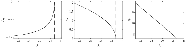
Figure 5. Normalized phase shift $\Delta_{b}$ (left), inverse width $\kappa_{b}$ (middle), and breather speed $c_{b}$ (right) versus $\lambda$ in $(-\infty,\lambda_{1}(k))$ for $k=0.8$. The band edge $\lambda_{1}(k)=-k^{2}$ is shown by the vertical dashed line.

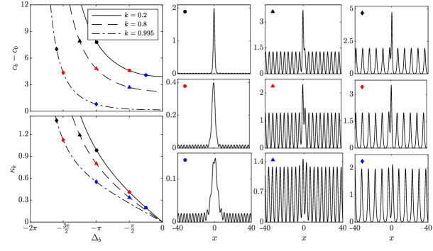
Figure 6. Left top (bottom): dependence of $c_{b}-c_{0}$ ($\kappa_{b}$) versus $\Delta_{b}$ for several values of $k$. Right: representative bright breather solutions. Representative solutions are marked on the left panel with a unique colored symbol.

Figure 6 characterizes the family of bright breathers by plotting $c_{b}-c_{0}$ and $\kappa_{b}$ versus $\Delta_{b}$ for three values of $k$. Profiles of representative breather solutions shown in Figure 6 confirm why we call them bright breathers. Bright breathers are more localized, have larger amplitudes, and move faster for smaller (more negative) values of $\Delta_{b}$ (smaller values of $\lambda$). For sufficiently large amplitude, $\Delta_{b}$ falls below $-\pi$ and the breather exhibits a positive phase shift $\Delta_{b}+2\pi\in(0,\pi]$ (cf. Remark 2). In contrast, for sufficiently small-amplitude breathers, $\Delta_{b}\in(-\pi,0)$ and the phase shift is negative.

7.1. Asymptotic limits $\lambda\to-\infty$ and $\lambda\to\lambda_{1}(k)$

It follows from (29) that

$$\varphi_{\gamma}=\left\{\begin{array}[]{ll}\displaystyle\frac{\pi}{2}-\frac{\sqrt{1-k^{2}}}{\sqrt{|\lambda|}}+\mathcal{O}(\sqrt{|\lambda|^{-3}})&\mbox{\rm as}\;\;\lambda\to-\infty,\\ \displaystyle\frac{\sqrt{|\lambda|-k^{2}}}{\sqrt{1-k^{2}}}+\mathcal{O}(\sqrt{(|\lambda|-k^{2})^{3}})&\mbox{\rm as}\;\;\lambda\to\lambda_{1}(k).\end{array}\right.$$

We also use the following asymptotic expansions of the elliptic integrals:

$$F(\varphi,k)=\varphi+\mathcal{O}(\varphi^{3}),\quad E(\varphi,k)=\varphi+\mathcal{O}(\varphi^{3}),\quad\mbox{\rm as}\;\;\varphi\to 0$$

and

$$F(\varphi,k)=K(k)+\mathcal{O}(\tfrac{1}{2}\pi-\varphi),\quad E(\varphi,k)=E(k)+\mathcal{O}(\tfrac{1}{2}\pi-\varphi),\quad\mbox{\rm as}\;\;\varphi\to\frac{\pi}{2}$$

The itemized list below summarizes the asymptotic results, where we use the asymptotic equivalence for the leading-order terms and neglect writing the remainder terms.

• The asymptotic values of the normalized phase shift $\Delta_{b}$ are

  $$\Delta_{b}\sim\left\{\begin{array}[]{ll}\displaystyle-2\pi+\frac{2\pi}{\sqrt{|\lambda|}K(k)}&\mbox{\rm as}\;\;\lambda\to-\infty,\\ \displaystyle-\frac{2\pi\sqrt{|\lambda|-k^{2}}}{\sqrt{1-k^{2}}K(k)}&\mbox{\rm as}\;\;\lambda\to\lambda_{1}(k).\end{array}\right.$$

  Since $\partial_{\varphi}F(\varphi,k)=(1-k^{2}\sin^{2}\varphi)^{-1/2}>0$ and $\partial_{\lambda}\varphi_{\gamma}<0$, the normalized phase shift $\Delta_{b}$ is a monotonically increasing function of $\lambda$ from $-2\pi$ to $0$. This proves that the map $\lambda\mapsto\Delta_{b}(\lambda)$ is one-to-one and onto from $(-\infty,\lambda_{1})$ to $(-2\pi,0)$.
  

• The asymptotic values for the inverse width $\kappa_{b}$ are

  $$\kappa_{b}\sim\left\{\begin{array}[]{ll}\displaystyle\sqrt{|\lambda|}&\mbox{\rm as}\;\;\lambda\to-\infty,\\ \displaystyle\sqrt{\frac{|\lambda|-k^{2}}{1-k^{2}}}\frac{E(k)}{K(k)}&\mbox{\rm as}\;\;\lambda\to\lambda_{1}(k).\end{array}\right.$$

  The derivative is given by

  $$\partial_{\lambda}\kappa_{b} =-\frac{\sin\varphi_{\gamma}}{2\sqrt{1-\lambda-k^{2}}}$$

  $$\quad+\Bigg{(}\sqrt{1-\lambda-k^{2}}\cos\varphi_{\gamma}-\sqrt{1-k^{2}\sin^{2}\varphi_{\gamma}}+\frac{E(k)}{K(k)\sqrt{1-k^{2}\sin^{2}\varphi_{\gamma}}}\Bigg{)}\partial_{\lambda}\varphi_{\gamma}.$$

  Since the terms in parentheses are positive and $\partial_{\lambda}\varphi_{\gamma}<0$, we have $\partial_{\lambda}\kappa_{b}<0$ so that $\kappa_{b}$ is a monotonically decreasing function of $\lambda$.
  

• The asymptotic values for the breather speed $c_{b}$ are

  $$c_{b}\sim\left\{\begin{array}[]{ll}\displaystyle\frac{4|\lambda|}{2-k^{2}-E(k)/K(k)}&\mbox{\rm as}\;\;\lambda\to-\infty,\\ \displaystyle c_{0}+4(1-k^{2})\frac{K(k)}{E(k)}&\mbox{\rm as}\;\;\lambda\to\lambda_{1}(k).\end{array}\right.$$

  The breather speed $c_{b}$ in (28) satisfies $c_{b}>c_{0}$. Based on the graphs in Fig. 5, we conjecture that the breather velocity $c_{b}$ is a decreasing function of $\lambda$.

7.2. Asymptotic limits $k\to 0$ and $k\to 1$

In the limit $k\to 0$, the background cnoidal wave $\phi_{0}(x)=2k^{2}{\rm cn}(x;k)$ vanishes since $\Theta(x)\to 1$ as $k\to 0$ whereas it follows from (27) and (28) that

$$\kappa_{b}\to\sqrt{|\lambda|},\qquad c_{b}\to 4|\lambda|,$$

since $Z(\varphi_{\gamma},k)\to 0$ and $c_{0}\to-4$ as $k\to 0$. The breather solution (5) with (6) recovers the one-soliton solution

$$u(x,t)\to 2|\lambda|\;\mathrm{sech}^{2}\left(\sqrt{|\lambda|}(x-4|\lambda|t+x_{0})\right),\quad k\to 0,$$

for every $\lambda\in(-\infty,0)$.

In the limit $k\to 1$, the background cnoidal wave $\phi_{0}(x)=2k^{2}{\rm cn}(x;k)$ transforms into the normalized soliton $\phi_{0}(x)\to 2\,{\rm sech}^{2}(x)$ and we will show that the breather solution (5) with (6) recovers the two-soliton solution. It follows from (27) and (28) that

$$\kappa_{b}\to\sqrt{|\lambda|},\qquad c_{b}\to 4|\lambda|,$$

since $Z(\varphi_{\gamma},k)\to 0$ and $c_{0}\to 4$ as $k\to 1$. Furthermore, it follows from (29) that $\varphi_{\gamma}\to\frac{\pi}{2}$ as $k\to 1$ so that $\alpha_{b}=F(\varphi_{\gamma},k)\to\infty$ as $k\to 1$. In order to regularize the solution, we use the translation invariance of the KdV equation, the $2K(k)$-periodicity of $\Theta$, and define the half-period translation of (6) with the transformation $x\to x-K(k)$, $x_{0}\to x_{0}+K(k)$:

$$\tau(x,t)=\Theta(x-c_{0}t+\alpha_{b}-K(k))e^{\kappa_{b}(x-c_{b}t+x_{0})}+\Theta(x-c_{0}t-\alpha_{b}+K(k))e^{-\kappa_{b}(x-c_{b}t+x_{0})}.$$ (36)

Recalling that $\alpha_{b}=F(\varphi_{\gamma},k)$, for each $\lambda\in(-\infty,-1)$, let us define the phase parameter $\delta_{b}$ by evaluating the limit [26, eq. (2.14)]:

$$\delta_{b}:=\lim_{k\to 1}\left[K(k)-F(\varphi_{\gamma},k)\right]=\frac{1}{2}\log\left(\frac{\sqrt{-\lambda}+1}{\sqrt{-\lambda}-1}\right).$$ (37)

It remains to deduce the asymptotic formula for $\Theta$ as $k\to 1$. We show that

$$\Theta(x)\sim\sqrt{\frac{-2k^{\prime}\log k^{\prime}}{\pi}}\cosh(x),\qquad\mbox{\rm as}\;\;k\to 1,$$ (38)

by using the Poisson summation formula [27]:

$$\Theta(x)=\sum_{n=-\infty}^{\infty}f(n)=\sum_{n=-\infty}^{\infty}\hat{f}(n),$$ (39)

where $\hat{f}(m)=\int_{-\infty}^{\infty}f(n)e^{-2\pi inm}dn$. Since

$$\Theta(x)=1+2\sum_{n=1}^{\infty}(-1)^{n}q^{n^{2}}\cos\left(\frac{n\pi x}{K(k)}\right),\qquad q:=e^{-\frac{\pi K(k^{\prime})}{K(k)}},$$

where $k^{\prime}=\sqrt{1-k^{2}}$, we obtain from (39) that

$$f(n)=q^{n^{2}}e^{in\pi\left(1+x/K(k)\right)},\quad\hat{f}(n)=\sqrt{\frac{K(k)}{K(k^{\prime})}}(q^{\prime})^{(n-1/2-x/2K(k))^{2}},$$ (40)

where $q^{\prime}:=e^{-\frac{\pi K(k)}{K(k^{\prime})}}$. As $k\to 1$, we have $k^{\prime}\to 0$ and

$$\begin{array}[]{l}K(k)=-\log{k^{\prime}}+2\log{2}+\mathcal{O}((k^{\prime})^{2}),\\ K(k^{\prime})=\frac{\pi}{2}+\frac{\pi}{8}k^{\prime 2}+\mathcal{O}((k^{\prime})^{4}),\\ q^{\prime}=\frac{1}{16}k^{\prime 2}+\frac{1}{32}k^{\prime 4}+\mathcal{O}((k^{\prime})^{6}).\end{array}$$

These expansions simplify (40) to

$$\hat{f}(n) =\sqrt{\frac{-2\log{k^{\prime}}}{\pi}}\left(\frac{k^{\prime}}{4}\right)^{\frac{(2n-1)^{2}}{2}}e^{(2n-1)x}\left(1+\frac{x^{2}-2\log{2}}{\log{k^{\prime}}}+\cdots\right),\quad\mbox{\rm as}\;\;k^{\prime}\to 0,$$

for every fixed $x\in\mathbb{R}$. Then, the rightmost summation in (39) yields the asymptotic expansion $\Theta(x)=\hat{f}(0)+\hat{f}(1)+\cdots$ in the form (38). Using it in (36), we obtain the asymptotic expansion

$$\tau(x,t)\sim\sqrt{\frac{-2k^{\prime}\log{k^{\prime}}}{\pi}}\Big{[}\cosh(\xi_{1}-\delta_{b})e^{\sqrt{|\lambda|}\xi_{2}}+\cosh(\xi_{1}+\delta_{b})e^{-\sqrt{|\lambda|}\xi_{2}}\Big{]},$$ (41)

where $\xi_{1}=x-4t$ and $\xi_{2}=x-4|\lambda|t+x_{0}$ for every $\lambda\in(-\infty,-1)$.

Using (41) with (37) in (5), we obtain the two-soliton solution in the form:

$$u(x,t)=2\frac{e^{2\delta_{b}}(1-\sqrt{|\lambda|})^{2}+e^{-2\delta_{b}}(1+\sqrt{|\lambda|})^{2}+2\cosh(2\sqrt{|\lambda|}\xi_{2})+2|\lambda|\cosh(2\xi_{1})}{[e^{\sqrt{|\lambda|}\xi_{2}}\cosh(\xi_{1}-\delta_{b})+e^{-\sqrt{|\lambda|}\xi_{2}}\cosh(\xi_{1}+\delta_{b})]^{2}}.$$

The two-soliton solution exhibits the asymptotic behavior

$$u(x,t)\sim\ 2\;\mathrm{sech}^{2}\left(\xi_{1}\mp\delta_{b}\right)+2|\lambda|\;\mathrm{sech}^{2}\left(\sqrt{|\lambda|}\xi_{2}\pm\delta_{b}\right),\quad\mbox{\rm as}\;\;t\to\pm\infty.$$

After the interaction, the slower soliton of amplitude 2 experiences the negative phase shift $-2\delta_{b},$ whereas the faster soliton of amplitude $2|\lambda|$ exhibits the positive phase shift $2\delta_{b}/\sqrt{|\lambda|}$.

8. Properties of the dark breather

Figure 7 plots $\Delta_{d}$, $\kappa_{d}$, and $c_{d}$ for dark breathers as a function of the parameter $\lambda$, see Theorem 2 and Remark 4. The phase shift $\Delta_{d}$ is monotonically decreasing between the band edges $\lambda_{2}(k)$ and $\lambda_{3}(k),$ shown by the vertical dashed lines. The inverse width $\kappa_{d}$ has a single maximum and vanishes at the band edges. The breather speed $c_{d}$ is monotonically decreasing. Since $c_{0}=-0.08$ for $k=0.7$, we confirm that $c_{d}<c_{0}$, which is also clear from Figure 2.

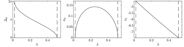
Figure 7. Normalized phase shift $\Delta_{d}$ (left), inverse width $\kappa_{d}$ (middle), and soliton speed $c_{d}$ (right) versus $\lambda$ in $(\lambda_{2}(k),\lambda_{3}(k))$ for $k=0.7$. The band edges $\lambda_{2}(k)=1-2k^{2}$ and $\lambda_{3}(k)=1-k^{2}$ are shown by the vertical dashed lines.

Figure 8 characterizes the family of dark breathers by plotting $c_{d}-c_{0}$ and $\kappa_{d}$ versus $\Delta_{d}$ for three values of $k$. The profiles of breather solutions at $t=0$ subject to the phase shift $x_{0}=5$ confirm why we refer to them as dark breathers. In contrast to the bright breather case, dark breather solutions exhibit vanishing cnoidal wave modulations for both of the extreme phase shifts $\Delta_{d}\to 0$ and $\Delta_{d}\to 2\pi$, with the largest-amplitude breather occurring at an intermediate phase shift, which we will later identify by examining the inverse width $\kappa_{d}$.

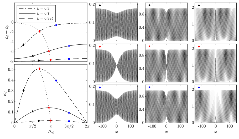
Figure 8. Left top (bottom): dependence of $c_{d}-c_{0}$ ($\kappa_{d}$) versus $\Delta_{d}$ for several values of $k$. Right: representative dark breather solutions. Representative solutions are marked on the left panel with a unique colored symbol. The dotted curve on the left panel corresponds to points of maximum $\kappa_{d}$ with the greatest localization.

8.1. Asymptotic limits $\lambda\to\lambda_{2}(k)$ and $\lambda\to\lambda_{3}(k)$

It follows from (34) that

$$\varphi_{\alpha}=\left\{\begin{array}[]{ll}\displaystyle\frac{\pi}{2}-\frac{\sqrt{\lambda-\lambda_{2}(k)}}{k}+\mathcal{O}\left(\lambda-\lambda_{2}\right)&\mbox{\rm as}\;\;\lambda\to\lambda_{2}(k),\\[8.53581pt] \displaystyle\frac{\sqrt{\lambda_{3}(k)-\lambda}}{k}+\mathcal{O}\left(\lambda_{3}-\lambda\right)&\mbox{\rm as}\;\;\lambda\to\lambda_{3}(k).\end{array}\right.$$

The itemized list below summarizes the asymptotic results, where we use the asymptotic equivalence for the leading-order terms and neglect writing the remainder terms.

• The asymptotic values of the normalized phase shift $\Delta_{d}$ are

  $$\Delta_{d}=\left\{\begin{array}[]{ll}\displaystyle 2\pi-\frac{2\pi}{K(k)}\sqrt{\frac{\lambda-\lambda_{2}(k)}{k^{2}(1-k^{2})}}&\mbox{\rm as}\;\;\lambda\to\lambda_{2}(k),\\ \displaystyle\frac{2\pi}{K(k)}\sqrt{\frac{\lambda_{3}(k)-\lambda}{k^{2}}}&\mbox{\rm as}\;\;\lambda\to\lambda_{3}(k).\end{array}\right.$$

  Since

  $$\partial_{\lambda}\Delta_{d}=\frac{2\pi}{K(k)}\partial_{\varphi_{\alpha}}F(\varphi_{\alpha},k)\partial_{\lambda}\varphi_{\alpha}$$

  with $\partial_{\varphi}F(\varphi,k)>0$ and $\partial_{\lambda}\varphi_{\alpha}<0$, the phase shift $\Delta_{d}$ monotonically decrease from $2\pi$ at $\lambda=\lambda_{2}(k)$ to $0$ at $\lambda=\lambda_{3}(k)$. This proves that the map $\lambda\mapsto\Delta_{d}(\lambda)$ is one-to-one and onto from $[\lambda_{2}(k),\lambda_{3}(k)]$ to $[0,2\pi]$.
  

• The asymptotic values of the inverse width $\kappa_{d}$ are

  $$\kappa_{d}=\left\{\begin{array}[]{ll}\displaystyle\left(\frac{E(k)}{K(k)}-1+k^{2}\right)\sqrt{\frac{\lambda-\lambda_{2}(k)}{k^{2}(1-k^{2})}}&\mbox{\rm as}\;\;\lambda\to\lambda_{2}(k),\\ \displaystyle\left(\frac{K(k)}{E(k)}-1\right)\frac{\sqrt{\lambda_{3}(k)-\lambda}}{k}&\mbox{\rm as}\;\;\lambda\to\lambda_{3}(k).\end{array}\right.$$

  The inverse width $\kappa_{d}=Z(\varphi_{\alpha},k)$ exhibits a maximum when [21, eq. 141.25]

  $$\sin\varphi_{\alpha}=\frac{1}{k}\sqrt{1-\frac{E(k)}{K(k)}}\quad\iff\quad\lambda=\lambda_{\rm max}(k):=\frac{E(k)}{K(k)}-k^{2}.$$

  The dark breather with this value of $\lambda$ can be interpreted as the narrowest (strongest) modulation of the cnoidal wave. Plotting the behavior of $\Delta_{\rm max}(k):=\Delta_{d}$ at $\lambda=\lambda_{\rm max}(k)$ as a function of $k$, we find that

  $$0<\Delta_{\rm max}(k)<\pi,$$

  with the upper limit reached as $k\to 0$. The dotted curve in the left top panel of Fig. 8 shows the graph of

  $$\left\{(\Delta_{\rm max}(k),c_{d}(\lambda_{\rm max}(k))-c_{0})\;\big{|}\;k\in(0,1)\right\}.$$

  Consequently, the most localized dark breather exhibits a positive phase shift. The phase shift is negative for $\lambda$ near $\lambda_{2}(k)$ since $\Delta_{d}-2\pi\in(-\pi,0)$ (cf. Remark 4) and is positive for $\lambda$ near $\lambda_{3}(k)$ since $\Delta_{d}\in(0,\pi)$. This partitions dark breathers into two branches: the slow (fast) branch for $0<\Delta_{d}<\Delta_{\rm max}(k)<\pi$ ($\Delta_{\rm max}(k)<\Delta_{d}<2\pi$). The slow branch exhibits dark breathers with strictly positive phase shifts whose amplitudes increase with increasing phase shift. On the fast branch, dark breathers can have positive or negative phase shift depending on whether $\Delta_{d}$ is less than or greater than $\pi$, respectively. Also, an increase in phase shift corresponds to a decrease in amplitude.
  

• The asymptotic values of the breather speed $c_{d}$ are

  $$c_{d}=\left\{\begin{array}[]{ll}\displaystyle c_{0}-\frac{4k^{2}(1-k^{2})}{E(k)/K(k)-1+k^{2}}&\mbox{\rm as}\;\;\lambda\to\lambda_{2}(k),\\ \displaystyle c_{0}-\frac{4k^{2}}{1-E(k)/K(k)}&\mbox{\rm as}\;\;\lambda\to\lambda_{3}(k).\end{array}\right.$$

  Based on the graphs in Fig. 7, we conjecture that the breather velocity $c_{d}$ is a monotonically decreasing function of $\lambda$.

8.2. Asymptotic limit $k\to 1$

We show similarly to Section 7.2 that the dark breather recovers the two-soliton solution in the limit $k\to 1$. The only difference from the degeration of the bright breather is that the spectral parameter $\lambda$ is now defined in $(-1,0)$ rather than in $(-\infty,-1)$. By using (38) in (7), we obtain the asymptotic approximation

$$\tau(x,t)\sim\sqrt{\frac{-2k^{\prime}\log{k^{\prime}}}{\pi}}\Big{[}\cosh(\xi_{1}+\delta_{d})e^{-\sqrt{|\lambda|}\xi_{2}}+\cosh(\xi_{1}-\delta_{d})e^{\sqrt{|\lambda|}\xi_{2}}\Big{]},\quad\mbox{\rm as}\;\;k\to 1,$$ (42)

where $\xi_{1}=x-4t$ and $\xi_{2}=x-4|\lambda|t+x_{0}$ for $\lambda\in(-1,0)$ and we have used $\kappa_{d}\to\sqrt{|\lambda|}$, $c_{d}\to 4|\lambda|$, and the corresponding limiting phase $\delta_{d}$ found from [26, eq. (2.7)]:

$$\delta_{d}:=\lim_{k\to 1}F(\varphi_{\alpha},k)=\frac{1}{2}\log\left(\frac{1+\sqrt{|\lambda|}}{1-\sqrt{|\lambda|}}\right),\quad\lambda\in(-1,0).$$ (43)

Inserting (42) and (43) into (5) results in the two-soliton solution

$$u(x,t)=2\frac{e^{2\delta_{d}}(1-\sqrt{|\lambda|})^{2}+e^{-2\delta_{d}}(1+\sqrt{|\lambda|})^{2}+2\cosh(2\sqrt{|\lambda|}\xi_{2})+2|\lambda|\cosh(2\xi_{1})}{[e^{-\sqrt{|\lambda|}\xi_{2}}\cosh(\xi_{1}+\delta_{d})+e^{\sqrt{|\lambda|}\xi_{2}}\cosh(\xi_{1}-\delta_{d})]^{2}},$$

that exhibits the asymptotic behavior

$$u(x,t)\sim\ 2\;\mathrm{sech}^{2}\left(\xi_{1}\pm\delta_{d}\right)+2|\lambda|\;\mathrm{sech}^{2}\left(\sqrt{|\lambda|}\xi_{2}\mp\delta_{d}\right),\quad t\to\pm\infty.$$

After the interaction, the slower soliton of amplitude $2|\lambda|$ experiences the negative phase shift $-2\delta_{d}/\sqrt{|\lambda|}$ whereas the faster soliton of amplitude $2$ exhibits the positive phase shift $2\delta_{d}$.

8.3. Asymptotic limit $k\to 0$

We show that the dark breather as $k\to 0$ can be approximated by a dark soliton solution of the nonlinear Schrodinger (NLS) equation.

In the limit $k\to 0$, the interval $[\lambda_{2}(k),\lambda_{3}(k)]$ shrinks to the point $\lambda=1$ and the solution $u(x,t)$ converges to the zero solution such that both the cnoidal wave and the dark breather vanish. For small $k$, it is well-known (see, e.g., [28]) that the multiple scales expansion

$$u(x,t) =2\mathrm{Re}\bigg{[}\epsilon\sqrt{\frac{\ell}{6}}A(\zeta,\tau)e^{i(\ell x-\omega t)}$$

$$\qquad\quad\,+\epsilon^{2}\frac{\ell}{6}\Big{(}\frac{1}{4}A(\zeta,\tau)^{2}e^{2i(\ell x-\omega t)}-\frac{1}{2}|A(\zeta,\tau)|^{2}\Big{)}+\mathcal{O}(\epsilon^{3})\bigg{]}$$ (44)

leads to the following NLS equation for the slowly varying amplitude $A(\zeta,\tau)$:

$$iA_{\tau}-\frac{1}{2}A_{\zeta\zeta}+|A|^{2}A=0,$$ (45)

where $0<\epsilon\ll 1$ is the amplitude parameter, $\ell>0$ is the carrier wavenumber, $\omega=-\ell^{3}$ is the KdV linear dispersion relation, and $\zeta=\frac{\epsilon}{\sqrt{6\ell}}(x+3\ell^{2}t)$ and $\tau=\epsilon^{2}t$ are slow variables. The NLS equation (45) admits the plane wave solution

$$A(\zeta,\tau)=e^{i(1+\frac{v^{2}}{2})\tau+iv\zeta+i\psi_{0}}$$ (46)

for any $v,\psi_{0}\in\mathbb{R}$. To determine $\ell$ and $\epsilon$, it is necessary to expand the cnoidal wave background of the dark breather solution for small elliptic modulus $0<k\ll 1$:

$$u(x,t) =2k^{2}{\rm cn}^{2}(x-c_{0}t)$$

$$=2k^{2}\cos^{2}(x-c_{0}t)+\mathcal{O}(k^{4})$$

$$=k^{2}+k^{2}\cos 2(x-c_{0}t)+\mathcal{O}(k^{4}),$$

where $c_{0}\to-4$ as $k\to 0$. The background cnoidal wave’s wavenumber $Q$, frequency $\Omega$, and mean value $\overline{\phi}$ expand as $k\to 0$ in the form:

$$\begin{array}[]{l}Q:=\frac{\pi}{K(k)}=2-\frac{k^{2}}{2}+\mathcal{O}(k^{4}),\\ \Omega:=c_{0}Q=-8+18k^{2}+\mathcal{O}(k^{4}),\\ \overline{\phi}:=\frac{1}{2K(k)}\int_{0}^{2K(k)}\phi_{0}(x)\,dx=k^{2}+\mathcal{O}(k^{4}).\end{array}$$

Comparing (44) with the asymptotic expansion for the background cnoidal wave, we find $\epsilon=\frac{k^{2}\sqrt{3}}{2}$ and $\ell=2$ confirming that the limit $k\to 0$ coincides with the NLS approximation. Since the expansion (44) does not incorporate an $\mathcal{O}(\epsilon)$ mean term, the Galilean transformation of the KdV equation can be used in (44) and (46) to obtain

$$u(x,t)\to k^{2}+u(x-6k^{2}t,t)=k^{2}+k^{2}\cos(\Lambda x-\Upsilon t+\psi_{0})+\mathcal{O}(k^{4}),$$ (47)

where

$$\begin{array}[]{l}\Lambda=2+\frac{v}{4}k^{2}+\mathcal{O}(k^{4}),\\ \Upsilon=-8+(12-3v)k^{2}+\mathcal{O}(k^{4}).\end{array}$$

The choice $v=-2$ asymptotically matches $\Lambda$ and $\Upsilon$ in (47) with $Q$ and $\Omega$.

The NLS equation (45) admits two families of dark soliton solutions [29]

$$A(\zeta,\tau)=\Big{(}\cos{\beta}\pm i\sin\beta\tanh\big{(}\sin\beta(\zeta-c_{\pm}\tau)\big{)}\Big{)}e^{i\left(-2\zeta+3\tau+\psi_{0}\right)},$$ (48)

where $\pm$ corresponds to the fast ($+$) and slow ($-$) solution branches with velocities $c_{\pm}=2\pm\cos{\beta}$, phase shift parameter $\beta\in[0,\pi/2]$, and arbitrary phase $\psi_{0}\in\mathbb{R}$. Since

$$A(\zeta,\tau)\to e^{i(-2\zeta+3\tau+\psi_{0}\mp\beta)}\quad\mbox{\rm as}\;\;\zeta-c_{\pm}\tau\to-\infty$$

and

$$A(\zeta,\tau)\to e^{i(-2\zeta+3\tau+\psi_{0}\pm\beta)}\quad\mbox{\rm as}\;\;\zeta-c_{\pm}\tau\to\infty,$$

the normalized phase shift is $\Delta_{\pm}:=\pm 2\beta$ for the fast ($-$) and slow ($+$) branch of solutions. Applying the Galilean transformation $u(x,t)\to k^{2}+u(x-6k^{2}t,t)$ to Eqs. (44) and (48), the dark soliton velocity-phase shift relation $c_{\pm}$ is

$$\begin{split}c_{\pm}=-12+\bigg{(}12+3\,\mathrm{sgn}(\Delta_{\pm})\cos\Big{(}\frac{\Delta_{\pm}}{2}\Big{)}\bigg{)}k^{2},\quad\Delta_{+}\in(0,\pi],\quad\Delta_{-}\in(-\pi,0).\end{split}$$ (49)

From Eq. (48), the inverse width parameter $\kappa_{\pm}:=\sin\frac{\beta\epsilon}{\sqrt{12}}$ is given by

$$\kappa_{\pm}=\frac{1}{4}\sin\left(\frac{|\Delta_{\pm}|}{2}\right)k^{2}.$$ (50)

In order to compare the dispersion relation given by (49) and (50) with the dark breather dispersion relation given by (32), (33), (35), we expand the spectral parameter $\lambda$ as $\lambda=1-k^{2}(1+\mu)$ with new scaled spectral parameter $\mu$, ensuring a distinct breather for each $\mu\in(0,1)$ as $k\to 0$. The small $k$ expansion of the dark breather dispersion relation (31), (32), (33), and (35) is given by

$$\begin{array}[]{l}\alpha_{d}=\arcsin(\sqrt{\mu})+\mathcal{O}(k^{2}),\\ \kappa_{d}=\frac{1}{2}\sqrt{\mu(1-\mu)}k^{2}+\mathcal{O}(k^{4}),\\ c_{d}=-12+(9+6\mu)k^{2}+\mathcal{O}(k^{4}),\\ \Delta_{d}=4\arcsin(\sqrt{\mu})+\mathcal{O}(k^{2}),\end{array}$$

for $\mu\in[0,1]$. Substituting $\mu=\sin^{2}\left(\frac{\Delta_{d}}{4}\right)$ yields

$$\begin{array}[]{l}c_{d}=-12+\left[12-3\cos\Big{(}\frac{\Delta_{d}}{2}\Big{)}\right]k^{2}+\mathcal{O}(k^{4}),\\ \kappa_{d}=\frac{1}{4}\sin\left(\frac{|\Delta_{d}|}{2}\right)k^{2}+\mathcal{O}(k^{4}).\end{array}$$ (51)

By identifying certain values of the phase shift $\Delta_{d}$ with the slow ($+$) and fast ($-$) branches of the NLS dark soliton solution (48), as given by

$$\Delta_{-}=\Delta_{d},\quad \Delta_{d}\in(0,\pi],$$

$$\Delta_{+}=\Delta_{d}-2\pi,\quad \Delta_{d}\in(-\pi,0),$$

we find that Eq. (51) coincides with Eqs. (49) and (50) up to and including the $\mathcal{O}(k^{2})$ terms. The fast and slow branches of the NLS dark soliton (48) coincide with the limiting fast and slow branches of the dark breather. The black soliton solution (48) with $\beta=\pi/2$ corresponds to the dark breather of maximum localization in which $\Delta_{\rm max}(k)\sim\pi$ as $k\to 0$.

9. Conclusion

A comprehensive characterization of explicit solutions of the KdV equation, representing the nonlinear superposition of a soliton and cnoidal wave, has been obtained using the Darboux transformation. These solutions are breathers, manifesting as nonlinear wavepackets propagating with constant velocity on a cnoidal, periodic, traveling wave background, subject to a topological phase shift. Breathers of elevation type, called bright breathers, are shown to propagate faster than the cnoidal background. Depression-type breathers are called dark breathers and they move slower than the cnoidal background. A key finding is that each breather on a fixed cnoidal wave background is uniquely determined by two distinct parameters: its initial position and a spectral parameter. We prove that the spectral parameter is in one-to-one correspondence with the normalized phase shift, which it imparts to the cnoidal background, in the interval $(-\pi,\pi].$

Bright breathers with small, negative phase shifts correspond to small-scale amplitude modulations of the cnoidal wave background, which result in the cnoidal wave dominating the solution. Small, positive phase shifts correspond to bright breathers with large-scale amplitude modulations of the cnoidal wave background where the soliton component is dominant. As the phase shift is swept across the interval $(-\pi,\pi]$, all breather amplitudes are attained.

In contrast, dark breather amplitudes, being of depression type, are limited. Small phase shifts, positive or negative, correspond to small modulations of the cnoidal wave background and the slow or fast branch of solutions, respectively. For each cnoidal wave background, we find a narrowest dark breather that imparts a positive phase shift. When the amplitude of the cnoidal wave background is small, dark breathers degenerate into dark soliton solutions of the NLS equation (45) derived from the KdV equation (1).

When the period of the cnoidal wave background goes to infinity, both bright and dark breather solutions are shown to degenerate into two-soliton solutions of the KdV equation. In this sense, breathers can be viewed as a generalization of two-soliton interactions. While such an interpretation is well-known for the sine-Gordon, focusing NLS, and the focusing modified KdV equations where breathers can be interpreted as bound states of two solitons [9], those breather solutions are localized. In contrast, the topological KdV breathers with an extended, periodic background described here represent a different class of nonlinear wave interaction solutions. We expect that such solutions exist for other integrable nonlinear evolutionary equations with a self-adjoint scattering problem such as the defocusing NLS and defocusing modified KdV equations.

An important application of these breather solutions is to the problem of soliton-dispersive shock wave (DSW) interaction [2]. Bright breathers were identified in [4] as being associated with soliton-DSW transmission. Soliton-DSW trapping corresponds to dark breathers embedding within the DSW. The spectral characterization of KdV breathers obtained here can be used in the context of multi-phase Whitham modulation theory [5] to describe the dynamics of breathers subject to large-scale amplitude modulations [4]. In addition to soliton-DSW interaction, the bright breathers resemble the propagation of a soliton through a special kind of deterministic soliton gas, constructed using Riemann-Hilbert methods from primitive potentials of the defocusing modified KdV equation [18]. Similar deterministic soliton gases have been identified as soliton condensates for the KdV equation [19] and provide further applications for the breathers constructed here.

Acknowledgement. The authors would like to thank the Isaac Newton Institute for Mathematical Sciences for support and hospitality during the programme Dispersive Hydrodynamics when work on this paper was undertaken (EPSRC Grant Number EP/R014604/1). The authors thank Y. Kodama and G. El for many useful suggestions on this project. MAH gratefully acknowledges support from NSF DMS-1816934.

$F(\varphi,k)$	Elliptic integral of the first kind $\displaystyle F(\varphi,k):=\int_{0}^{\varphi}\frac{d\alpha}{\sqrt{1-k^{2}\sin^{2}\alpha}}$
$E(\varphi,k)$	Elliptic integral of the second kind $\displaystyle E(\varphi,k):=\int_{0}^{\varphi}\sqrt{1-k^{2}\sin^{2}\alpha}d\alpha$
$K(k)$	Complete elliptic integral $\displaystyle K(k):=F\left(\frac{\pi}{2},k\right)$
$E(k)$	Complete elliptic integral $\displaystyle E(k):=E\left(\frac{\pi}{2},k\right)$
$Z(\varphi,k)$	Zeta function $\displaystyle Z(\varphi,k):=E(\varphi,k)-\frac{E(k)}{K(k)}F(\varphi,k)$
${\rm sn}(x,k)$	Jacobi elliptic function ${\rm sn}(x,k)=\sin\varphi$
${\rm cn}(x,k)$	Jacobi elliptic function ${\rm cn}(x,k)=\cos\varphi$
${\rm dn}(x,k)$	Jacobi elliptic function ${\rm dn}(x,k)=\sqrt{1-k^{2}\sin^{2}\varphi}$
$H(x)$	$\theta_{1}\left(\frac{\pi x}{2K(k)}\right)$ with $\displaystyle\theta_{1}(u)=2\sum\limits_{n=1}^{\infty}(-1)^{n-1}q^{(n-\frac{1}{2})^{2}}\sin(2n-1)u$
$H_{1}(x)$	$\theta_{2}\left(\frac{\pi x}{2K(k)}\right)$ with $\displaystyle\theta_{2}(u)=2\sum\limits_{n=1}^{\infty}q^{(n-\frac{1}{2})^{2}}\cos(2n-1)u$
$\Theta_{1}(x)$	$\theta_{3}\left(\frac{\pi x}{2K(k)}\right)$ with $\displaystyle\theta_{3}(u)=1+2\sum\limits_{n=1}^{\infty}q^{n^{2}}\cos 2nu$
$\Theta(x)$	$\theta_{4}\left(\frac{\pi x}{2K(k)}\right)$ with $\displaystyle\theta_{4}(u)=1+2\sum\limits_{n=1}^{\infty}(-1)^{n}q^{n^{2}}\cos 2nu$
$q$	$\displaystyle e^{-\frac{\pi K^{\prime}(k)}{K(k)}}$ with $K^{\prime}(k)=K(k^{\prime})$ and $k^{\prime}=\sqrt{1-k^{2}}$

Table 1. Table of elliptic integrals and Jacobi elliptic functions.

References

• [1] V.B. Matveev and M. A. Salle, Darboux Transformations and Solitons (Springer-Verlag, Berlin, 1991).
• [2] M. D. Maiden, D. V. Anderson, A. A. Franco, G. A. El, and M. A. Hoefer, “Solitonic dispersive hydrodynamics: Theory and observation,” Phys. Rev. Lett. 120 (2018) 144101
• [3] P. Sprenger, M. A. Hoefer, and G. A. El, “Hydrodynamic optical soliton tunneling”, Phys. Rev. E 97 (2018) 032218
• [4] M. J. Ablowitz, J. T. Cole, G. A. El, M. A. Hoefer, and X. Luo, “Soliton-mean field interaction in Korteweg-de Vries dispersive hydrodynamics,” arXiv:221.14884 (2022)
• [5] H. Flaschka, M. G. Forest, and D. W. McLaughlin, “Multiphase averaging and the inverse spectral solution of the Korteweg-de Vries equation,” Comm. Pure Appl. Math. 33 (1980) 739–784
• [6] G. A. El and M. A. Hoefer, “Dispersive shock waves and modulation theory”, Physica D 333 (2016) 11–65
• [7] M. J. Ablowitz, X. D. Luo, and J. T. Cole, “Solitons, the Korteweg–de Vries equation with step boundary values, and pseudo-embedded eigenvalues”, J. Math. Phys. 59 (2018), 091406 (14 pages).
• [8] A. Mucalica and D.E. Pelinovsky, “Solitons on the rarefaction wave background via the Darboux transformation”, Proc. R. Soc. A 478 (2022) 20220474 (17 pages)
• [9] M. J. Ablowitz and H. Segur, Solitons and the Inverse Scattering Transform (SIAM, Philadelphia, 1981)
• [10] S. Clarke, R. Grimshaw, P. Miller, E. Pelinovsky, and T. Talipova, “On the generation of solitons and breathers in the modified Korteweg–de Vries equation”, Chaos 10 (2000) 383.
• [11] E. A. Kuznetsov and A. V. Mikhailov, “Stability of stationary waves in nonlinear weakly dispersive media”, Sov. Phys. JETP 40 (1974) 855–859
• [12] X. R. Hu, S. Y. Lou, and Y. Chen, “Explicit solutions from eigenfunction symmetry of the Korteweg–de Vries equation”, Phys. Rev. E 85 (2012) 056607
• [13] E. D. Belokolos, A. I. Bobenko, V. Z. Enol’skii, A. R. Its, and V. B. Matveev, Algebro-Geometric Approach to Nonlinear Integrable Equations (Springer-Verlag, Berlin, 1994)
• [14] F. Gesztesy and R. Svirsky, “(m)KdV solitons on the background of quasi-periodic finite-gap solutions”, Mem. Amer. Math. Soc. 118 (1995), 563 (88 pages)
• [15] A. Nakayashiki, “One step degeneration of trigonal curves and mixing of solitons and quasi-periodic solutions of the KP equation”, in Geometric methods in physics XXXVIII (Birkhäuser/Springer, Cham, 2020), pp. 163–186.
• [16] J. Bernatska, V. Enolski, and A. Nakayashiki, “Sato Grassmannian and degenerate sigma function”, Commun. Math. Phys. 374 (2020) 627–660
• [17] M. Bertola, R. Jenkins, and A. Tovbis, “Partial degeneration of finite gap solutions to the Korteweg–de Vries equation: soliton gas and scattering on elliptic background”, arXiv: 2210.01350 (2022)
• [18] M. Girotti, T. Grava, R. Jenkins, K. McLaughlin, and A. Minakov, “Soliton v. the gas: Fredholm determinants, analysis, and the rapid oscillations behind the kinetic equation,” arXiv:2205.02601 (2022).
• [19] T. Congy, G. A. El, G. Roberti, and A. Tovbis, “Dispersive hydrodynamics of soliton condensates for the Korteweg-de Vries equation,” arXiv:2208.04472 (2022)
• [20] C. S. Gardner, J. M. Greene, M. D. Kruskal, and R. M. Miura, “Method for solving the Korteweg-de Vries equation,” Phys. Rev. Lett. 19 1095–-1097 (1967).
• [21] P. F. Byrd and M. D. Friedman, Handbook of Elliptic Integrals for Engineers and Scientists, 2nd Edition (Springer-Verlag, Berlin, 1971).
• [22] I. S. Gradshteyn and I. M. Ryzhik, Table of Integrals, Series, and Products (Academic Press, New York, 2007)
• [23] D. F. Lawden, Elliptic Functions and Applications, Appl. Math. Sci. 80 (Springer, New York, 1989)
• [24] E. L. Ince, Ordinary Differential Equations (Dover Publications, New York, 1956)
• [25] B. Oblak, “ Orbital bifurcations and shoaling of cnoidal waves,” J. Math. Fluid Mech. 22 (2020) 29
• [26] H. Van de Vel, “On the series expansion method for computing incomplete elliptic integrals of the first and second kinds”, Math. Comp. 23 (1969) 61–69
• [27] J. P. Boyd, “Theta functions, Gaussian series, and spatially periodic solutions of the Korteweg–de Vries equation”, J. Math. Phys. 23 (1982) 375
• [28] V. E. Zakharov and E. A. Kuznetsov, “Multi-scale expansions in the theory of systems integrable by the inverse scattering transform,” Physica D 18 (1986) 455–463
• [29] M. J. Ablowitz, Nonlinear Dispersive Waves: Asymptotic Analysis and Solitons (Cambridge University Press, Cambridge, 2011)