DynInt: Dynamic Interaction Modeling for Large-scale Click-Through Rate Prediction

Abstract.

Learning feature interactions is the key to success for the large-scale CTR prediction in Ads ranking and recommender systems. In industry, deep neural network-based models are widely adopted for modeling such problems. Researchers proposed various neural network architectures for searching and modeling the feature interactions in an end-to-end fashion. However, most methods only learn static feature interactions and have not fully leveraged deep CTR models’ representation capacity. In this paper, we propose a new model: DynInt. By extending Polynomial-Interaction-Network (PIN), which learns higher-order interactions recursively to be dynamic and data-dependent, DynInt further derived two modes for modeling dynamic higher-order interactions: dynamic activation and dynamic parameter. In dynamic activation mode, we adaptively adjust the strength of learned interactions by instance-aware activation gating networks. In dynamic parameter mode, we re-parameterize the parameters by different formulations and dynamically generate the parameters by instance-aware parameter generation networks. Through instance-aware gating mechanism and dynamic parameter generation, we enable the PIN to model dynamic interaction for potential industry applications. We implement the proposed model and evaluate the model performance on real-world datasets. Extensive experiment results demonstrate the efficiency and effectiveness of DynInt over state-of-the-art models.

1. Introduction

Click-through rate (CTR) prediction model (Richardson et al., 2007) is an essential component for the large-scale search ranking, online advertising and recommendation system (McMahan et al., 2013; He et al., 2014; Cheng et al., 2016; Zhang et al., 2019).

Many deep learning-based models have been proposed for CTR prediction problems in the industry and have become dominant in learning the useful feature interactions of the mixed-type input in an end-to-end fashion(Zhang et al., 2019). While most of the existing methods focus on automatically modeling static deep feature representations, there are very few efforts on modeling feature representations dynamically.

However, the static feature interaction learning methods may not fully fulfill the complexity and long-tail property of large-scale search ranking, online advertising, and recommendation system problems. The static feature interaction learning can not capture the characteristics of long-tail instances effectively and efficiently, as short-tail instances and high-frequency features will easily dominate the shared and static parameters of the model. Therefore, we argue that the learned feature interactions should be dynamic and adaptive to different instances for capturing the pattern of long-tail instances.

Inspired by the dynamic model framework, we propose a dynamic feature interaction learning method called DynInt. DynInt has two schemes that enhance the base model (xDeepInt (Yan and Li, 2020)) to learn the dynamic and personalized interactions.

• DynInt-DA: We reinforce the Polynomial-Interaction-Network by instance-aware activation gating networks for adaptively refining learned interactions of different s.

• DynInt-DGP and DynInt-DWP: We re-parametrize the parameters of Polynomial-Interaction-Network by instance-aware parameter generation networks for adaptively generating and re-weighting the parameters to learn dynamic interactions.

• We introduce the different computational paradigms to reduce the memory cost and improve efficiency in implementations effectively.

• We introduce the orthogonal regularization for enhancing the diversity of learned representation in dynamic interaction modeling settings.

• We conduct extensive experiments on real-world datasets and study the effect of different hyper-parameters, including but not limited to: kernel size, latent rank, and orthogonal regularization rate.

2. Related Work

2.1. Static Interaction Modeling

Most deep CTR models map the high-dimensional sparse categorical features and continuous numerical features onto a low dimensional latent space as the initial step. Many existing model architectures focus on learning static implicit/explicit feature interactions simultaneously.

Various hybrid network architectures (Cheng et al., 2016; Qu et al., 2016, 2018; Wang et al., 2017, 2021b; Guo et al., 2017; Lian et al., 2018) utilize feed-forward neural network with non-linear activation function as its deep component, to learn implicit interactions. The complement of the implicit interaction modeling improves the performance of the network that only models the explicit interactions (Beutel et al., 2018). However, this type of approach fails to bound the degree of the learned interactions.

Deep & Cross Network (DCN) (Wang et al., 2017) and its improved version DCN V2  (Wang et al., 2021b) explores the feature interactions at the bit-wise level explicitly in a recursive fashion. Deep Factorization Machine (DeepFM) (Guo et al., 2017) utilizes factorization machine layer to model the pairwise vector-wise interactions. Product Neural Network (PNN) (Qu et al., 2016, 2018) introduces the inner product layer and the outer product layer to learn vector-wise interactions and bit-wise interactions, respectively. xDeepFM (Lian et al., 2018) learns the explicit vector-wise interaction by using Compressed Interaction Network (CIN), which has an RNN-like architecture and learns vector-wise interactions using Hadamard product. FiBiNET (Huang et al., 2019) utilizes Squeeze-and-Excitation network to dynamically learn the importance of features and model the feature interactions via bilinear function. AutoInt (Song et al., 2018) leverages the Transformer (Vaswani et al., 2017) architecture to learn different orders of feature combinations of input features. xDeepInt (Yan and Li, 2020) utilizes polynomial interaction layer to recursively learn higher-order vector-wise and bit-wise interactions jointly with controlled degree, dispensing with jointly-trained DNN and nonlinear activation functions.

2.2. Gating Mechanism in Deep Learning

Gating mechanism is widely used in computer vision and natural language processing, more importantly, CTR prediction for Ads ranking and recommendation systems.

LHUC (Swietojanski and Renals, 2014) learns hidden unit contributions for speaker adaptation. Squeeze-and-Excitation Networks (Hu et al., 2018) recalibrates channel-wise feature responses by explicitly modeling interdependencies and multiplying each channel with learned gating values. Gated linear unit (GLU) (Dauphin et al., 2017) was utilized to control the bandwidth of information flow in language modeling.

Multi-gate Mixture-of-Experts (MMoE) (Ma et al., 2018) utilizes gating networks to automatically weight the representation of shared experts for each task, so that simultaneously modeling shared information and modeling task specific information. GateNet (Huang et al., 2020) leverages feature embedding gate and hidden gate to select latent information from the feature-level and intermediate representation level, respectively. MaskNet (Wang et al., 2021a) introduces MaskBlock to apply the instance-guided mask on feature embedding and intermediate output. The MaskBlock can be combined in both serial and parallel fashion. Personalized Cold Start Modules (POSO) (Dai et al., 2021) introduce user-group-specialized sub-modules to reinforce the personalization of existing modules, for tackling the user cold start problem. More specifically, POSO combines the personalized gating mechanism with existing modules such as Multi-layer Perceptron, Multi-head Attention, and Multi-gated Mixture of Experts, and effectively improves their performance.

2.3. Parameter Generation in Deep Learning

Besides adjustments on feature embedding and intermediate representations, dynamic parameter generation is more straightforward in making the neural network adaptive to the input instance.

Dynamic filter networks (DFN) (Jia et al., 2016) and HyperNetworks (Ha et al., 2016) are two classic approaches for runtime parameter generation for CNNs and RNNs, respectively. DynamicConv (Wu et al., 2019), which is simpler and more efficient, was proved to perform competitively to the self-attention.

In the recommendation area, PTUPCDR (Zhu et al., 2022) leverages meta network fed with users’ characteristic embeddings to generate personalized bridge functions to achieve personalized transfer for cross domain recommendation. Co-Action Network (CAN) (Bian et al., 2022) uses learnable item embedding as parameters of micro-MLP to realize interaction with user historical behavior sequence, for approximating the explicit and independent pairwise feature interactions without introducing too many additional parameters. Adaptive Parameter Generation network (APG) (Yan et al., 2022) re-parameterize the dense layer parameters of deep CTR models with low-rank approximation, where the specific parameters are dynamically generated on-the-fly based on different instances.

3. Proposed Model: Dynamic Interaction Network (DynInt)

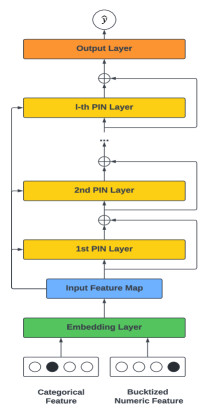
Figure 1. The architecture of unrolled Polynomial Interaction Network with residual connections

In this section, we give an overview of the architectures of DynInt variants. We first clarify the notations. $F$ is the number of features. $i$ is the instance index. $j$ is the feature index. $D$ is the feature embedding size. $K$ is the rank of the approximation. $B$ is the batch size. $X_{0}$ is the input feature map and $X_{l}$ is the $l$-th layer output. $W_{l}$ is the $l$-th layer parameter matrix.

Our models first embed each feature into a dense embedding vector $x_{j}$ of dimension $D$. We denote the output of embedding layer $X_{0}\in R^{F\times D}$ as the input feature map:

(1) $$X_{0}=[x_{0},x_{1},\cdots,x_{F-1}]^{\intercal}.$$

The shared components of all the DynInt model variants are from the xDeepInt (Yan and Li, 2020). The key components of the xDeepInt, as illustrated in Figure 2, include Polynomial Interaction Network(PIN) layers, Subspace-crossing Mechanism, and GroupLasso-FTRL/FTRL composite optimization strategy:

• The PIN layer can capture the higher-order polynomial interactions and is the backbone of our architectures.

• The Subspace-crossing Mechanism enables the PIN to learn both vector-wise and bit-wise interactions while controlling the degree of mixture between vector-wise interactions and bit-wise interactions. As shown in the 2(b), By the Subspace-crossing Mechanism, One can choose to fully retain the field-level semantic information and only explore vector-wise interaction between features. One can also model the bit-wise interactions by splitting the embedding space into $h$ sub-spaces.

• The GroupLasso-FTRL/FTRL composite optimization strategy takes advantage of the properties of different optimizers: GroupLasso-FTRL achieves row-wise sparsity for embedding table, and FTRL achieves element-wise sparsity for weight parameters, as shown in 2(c).

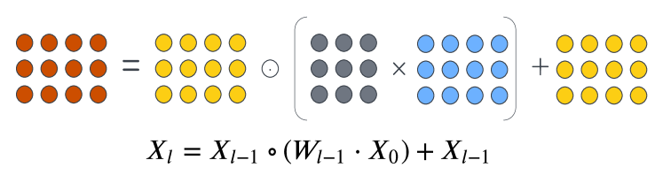
(a) Polynomial Interaction Network (PIN) Layer

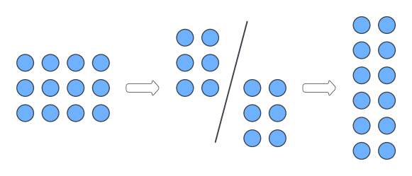
(b) Subspace-crossing Mechanism

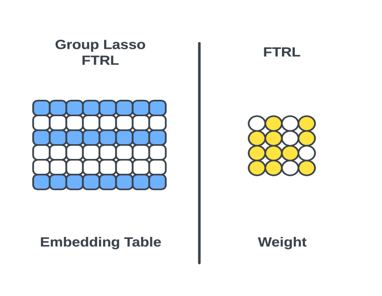
(c) GroupLasso FTRL v.s. FTRL

Figure 2. The key components of the xDeepInt model

The output layer of DynInt model variants is merely a dense layer applied to the feature dimension. The output of PIN is a feature map that consists different degree of feature interactions, including input feature map preserved by residual connections and higher-order feature interactions learned by PIN. The output layer work as:

(2) $$\hat{y} =\sigma\big{(}(W_{out}X_{l}+b_{out}\mathbf{1}^{T})\mathbf{1}\big{)}$$

where $\sigma$ is the sigmoid function, $W_{out}\in R^{1\times F}$ is an aggregation vector that linearly combines all the learned feature interactions, and $b\in R$ is the bias.

We will mainly focus on enhancing the architecture of PIN layer such that the models become instance-aware. Therefore, we will mainly focus on the enhancement of the PIN layer. For simplicity in notations, the subspace-crossing mechanism will not be included in the model introduction and will be included in the implementation for the model performance.

3.1. Polynomial Interaction Network

We first go through the architecture of the PIN layer. The mathematical representation of the $l$-th PIN layer with residual connection is given by

(3) $$X_{l}=X_{l-1}\circ(W_{l-1}\cdot X_{0})+X_{l-1}$$

As 2(a) illustrated, $X_{l}$ is the $l$-th layer output of PIN. $X_{l}\in R^{F\times D}$, where $F$ is the number of features, and $D$ is the embedding dimension. $W_{l}\in R^{F\times F}$ is the static parameter that is shared across different instances.

In order to improve the representation power of PIN, we enable the PIN layer parameters to be instance-aware, which enables the dynamic vector-wise and bit-wise interactions modeling. We propose two formulations as follows.

3.2. Dynamic Activation (DynInt-DA)

The first scheme is to add dynamic mechanism to the output of each PIN layer.

(4) $$X_{l}=\Big{(}X_{l-1}\circ(W_{l-1}\cdot X_{0})\Big{)}\circ G_{l-1}^{(i)}+X_{l-1}$$

We multiply the output of the $l$-th layer by a instance-aware gating vector $G_{l}^{(i)}$. The gating vector $G_{l}^{(i)}$ can be modeled by a two-layer DNN with reduction ratio $r$, using $X_{0}$ as input.

Empirically, we find that the initialized values of $G_{l}^{(i)}$ around 1.0 result in better convergence. We set the activation function of gating network as: $\text{Sigmoid}(x)*2.0$. By using this activation function, we have the $G_{l}^{(i)}$ initialized around 1.0 when using zero-mean initialization for DNN layer parameters. Meanwhile, we use the input feature map $X_{0}$ as the input of our gating network, which models the dynamic gate for each PIN layer’s outputs.

During the training phase, the input feature map $X_{0}$ does not receive gradients from the gating network to ensure training stability. Figure 3 illustrates the architecture of the enhanced PIN layer of the DynInt-DA model.

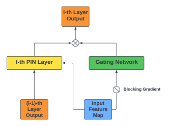
Figure 3. PIN Layer with Dynamic Activation.

3.3. Dynamic Parameters (DynInt-DP)

Dynamic parameters scheme is to dynamically model $W_{l-1}$ at each PIN layer. We propose two formulations to model the dynamic parameters.

3.3.1. Dynamic Generated Parameters (DynInt-DGP)

Instead of using the static parameters, we allow parameter matrices to be data-dependent.

(5) $$X_{l}=X_{l-1}\circ(W^{(i)}_{l-1}\cdot X_{0})+X_{l-1}$$

$W^{(i)}_{l-1}$ is a dynamic parameter matrix for the $i$-th instance.

3.3.2. Dynamic Weighted Parameters (DynInt-DWP)

Let $G^{(i)}_{l-1}$ be a dynamic weighting matrix for the $i$-th instance. We replace the static parameter matrix $W_{l-1}$ with the Hadamard product of the dynamic weighting matrix $G^{(i)}_{l-1}$ and the static parameter matrix $W_{l-1}$ and obtain that

(6) $$X_{l}=X_{l-1}\circ\big{(}(G^{(i)}_{l-1}\circ W_{l-1}\cdot X_{0})\big{)}+X_{l-1}$$

In DGP and DWP, the dynamic parameter matrices $W_{l-1}^{(i)}$ and dynamic weighting matrices $G_{l-1}^{b}$ can also be estimated by two-layer DNNs with reduction ratio $r$. If we take the batch size into consideration, the backward propagation needs to compute the gradients of the matrices of the size $B\times F\times F$, which results in extremely high memory cost. Direct implementations of DWP and DGP are implausible in practice. In the next section, we propose two computation paradigms to implement DGP and DWP with lower memory cost.

3.4. Low-Rank Approximation for Dynamic Parameters

The Low-Rank Approximation is commonly used to reduce the memory and computation cost. In PIN layer, we explore the singular values of the trained parameter matrix $W_{l}$. As shown in Figure 5, the singular values drop dramatically.

This phenomenon indicates that most of the information is condensed in the top singular values and vectors. Therefore, the low-rank approximation of the parameters can effectively reconstruct the parameters while also improving the serving efficiency.

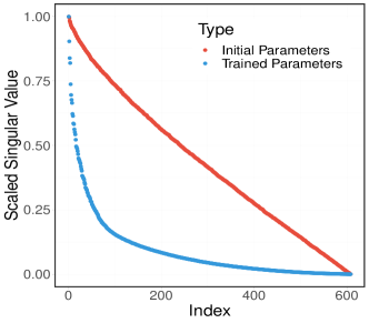
Figure 4. The singular values of the trained parameter matrix $W_{l}$. We observed that the scaled singular values of the trained static parameter matrices shows a elbow shape, which indicates that the low rank approximation of the parameter matrices preserves the majority of the information.

3.5. Computational Paradigms of Dynamic Parameters Formulations

The computational paradigms assume the dynamic parameter matrix or weighting matrix has low ranks, which controls the model complexity and simplifies the computation. Based on this assumption, we apply singular value decomposition (SVD) to these dynamic matrices.

3.5.1. Dynamic Generated Parameters

Suppose we have a rank-K approximation of the dynamic parameter matrix $W_{l-1}^{(i)}$

(7) $$W_{l-1}^{(i)}=U_{l-1}\cdot\Sigma_{l-1}^{(i)}\cdot V_{l-1}^{T}$$

where $U_{l-1}\in R^{F\times K}$, $\Sigma_{l-1}^{(i)}\in R^{K\times K}$ and $V_{l-1}\in R^{F\times K}$. We let the singular value matrices be adaptive to instance. Thus all instances will share the same vector space spanned by $U_{l-1}$ and $V_{l-1}$. It can be viewed as a regularization trick. Then $W_{l-1}^{(i)}\cdot X_{0}$ in eq. 5 can be written as:

(8) $$U_{l-1}\cdot\Sigma_{l-1}^{(i)}\cdot V_{l-1}^{T}\cdot X_{0}$$

Since $U_{l-1}$ and $V_{l-1}$ are shared static parameters across all instances. Thus we only need to store two matrices of size $F\times K$ and $B$ diagonal matrices of size $K\times K$ during the forward propagation. Since $\Sigma_{l-1}^{(i)}$ is data-dependent, we will use a two-layer DNN with reduction ratio $r$, with $X_{0}$ as input to model the non-zero diagonal entries of $\Sigma_{l-1}^{(i)}$. Similar to DynInt-DA, we blocked the gradient of $X_{0}$ to prevent co-adaption issue.

5(a) shows how we decompose the $W_{l-1}$ with static parameter $U_{l-1}$ and $V_{l-1}$, and instance-aware dynamic parameter $\Sigma_{l-1}^{(i)}$.

3.5.2. Dynamic Weighted Parameters

Suppose ${G}^{(i)}_{l-1}$ is the $(l-1)$-th layer weighting matrix has rank K. Then ${G}^{(i)}_{l-1}$ has a SVD of the form

(9) $$\mathbf{G}^{(i)}_{l-1}=\sum_{p=1}^{K}\tilde{\mathbf{u}}^{(i)}_{p,l-1}\tilde{\mathbf{v}}^{(i)}_{p,l-1}$$

where $\tilde{\mathbf{u}}^{(i)}_{p,l-1}=\sqrt{\sigma_{p,l-1}^{(i)}}\mathbf{u}_{p,l-1}^{(i)}$ and $\tilde{\mathbf{v}}_{p,l-1}^{(i)}=\sqrt{\sigma_{p,l-1}^{(i)}}\mathbf{v}^{(i)}_{p,l-1}$. $\tilde{\mathbf{u}}_{p,l-1}^{(i)}$ and $\mathbf{v}_{p,l-1}^{(i)}$ are unit-norm vectors that satisfy that $\tilde{\mathbf{u}}^{(i)}_{p,l-1}\perp\tilde{\mathbf{v}}^{(i)}_{p,l-1}$ for all p’s. Therefore, the PIN layer with dynamic parameters can be re-written as

(10) $$X_{l} =\sum_{p=1}^{K}X_{l-1}\circ\Big{(}\big{(}\textbf{diag}(\tilde{\mathbf{u}}^{(i)}_{p,l-1})\cdot W_{l-1}\cdot\textbf{diag}(\tilde{\mathbf{v}}^{(i)}_{p,l-1})\big{)}\cdot X_{0}\Big{)}+X_{l-1}$$

where $\tilde{\mathbf{u}}^{(i)}_{p,l-1}\perp\tilde{\mathbf{v}}^{(i)}_{p,l-1}$ for all p’s. We simplify the Hadamard product to the matrix product. And $W_{l-1}$ is the shared parameter matrix in this formulation. $\tilde{\mathbf{u}}^{(i)}_{p,l-1}$ and $\tilde{\mathbf{v}}^{(i)}_{p,l-1}$ are the personalized weights. Since we can simplify the hadmard product of a rank-1 matrix and a matrix with a row-wise broadcasting operation and a column-wise broadcasting operation, we apply the vectorized form to the DWP. In each forward propagation iteration, $K$ pairs $\tilde{\mathbf{u}}^{(i)}_{p,l-1}$, $\tilde{\mathbf{v}}^{(i)}_{p,l-1}$ and a shared parameter matrix $W_{l-1}$ will be stored.

5(b) illustrates the decomposition of dynamic weighting matrix $\mathbf{G}^{(i)}_{l-1}$. The $K$ pairs $\tilde{\mathbf{u}}^{(i)}_{p,l-1}$, $\tilde{\mathbf{v}}^{(i)}_{p,l-1}$ are modeled by a two-layer DNN network with reduction ratio $r$ and using gradient blocked $X_{0}$ as input, similar to aforementioned setup. Since we want to ensure the entries of $\mathbf{G}^{(i)}_{l-1}$ is around 1.0 after initilization, we add $1.0/K$ to the output of the DNN that modeling $K$ pairs $\tilde{\mathbf{u}}^{(i)}_{p,l-1}$, $\tilde{\mathbf{v}}^{(i)}_{p,l-1}$. We find this trick improves the training stability.

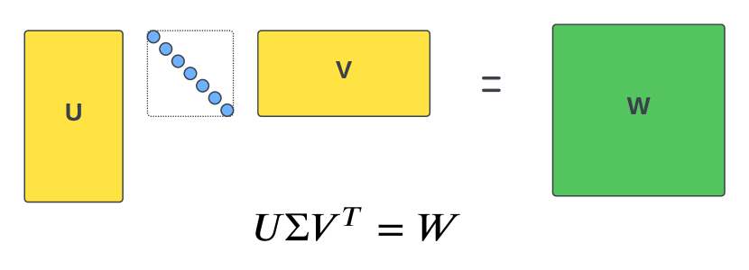
(a) Low rank approximations of dynamic parameter matrices $W$. In implementation, we let $U$ and $V$ to be static parameters. $\Sigma$ is dynamic parameters.

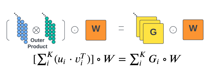
(b) Low rank approximations of the dynamic weighting matrices $G$. In implementation, we let $u_{i}$ and $v_{i}$ to be dynamic parameters.

Figure 5. Low rank approximation for two dynamic parameters formulation. Both $DGP$ and $DWP$ use SVD to approximate the dynamic parameter matrices(DGP) or dynamic weighting matrices(DWP).

3.5.3. Memory Cost Reduction

For both DynInt-DWP and DynInt-DGP, the memory cost for the instance-aware parameter matrix is $B\times F\times F$. For the DynInt-DGP with the proposed computation paradigm, the memory cost of the low-rank approximation of the parameter matrix is $B\times K\times K$ + $2\times F\times K$ with $K<<F$. If $K=\frac{1}{10}F$, the memory cost for storing the personalized weighted matrix is reduced by $99\%$ with the proposed computation paradigm. For the the DynInt-DWP with the proposed computation paradigm, the memory cost of the low-rank approximation of the parameter matrix is $2\times B\times F\times K+F\times F$ with $K<<F$. If $K=\frac{1}{10}F$, the memory cost for storing the personalized weighted matrix is reduced by $80\%$.

3.5.4. FLOPs Analysis

DynInt-DGP requires $O(F\times F\times D)$ FLOPs for each instance. With SVD, the computational cost can be reduced to $O(2\times F\times K\times K+F\times K\times D)$, the flops of SVD is significantly smaller than $O(F\times F\times D)$ given $K<<D,F$. DynInt-DWP also requires $O(F\times F\times D)$ FLOPs for each instance. With SVD, the computational cost is $O(2K\times F\times F+K\times F\times F\times D)$ which is comparable with $O(F\times F\times D)$ when $K<<D,F$

Therefore, the proposed computation paradigms can significantly reduce the memory cost. DGP can also reduce the computational cost with the proposed computational paradigm.

3.6. Orthogonal Regularization and Loss Function

Both computational paradigms are based on low-rank approximations and SVD. While we model the instance-aware dynamic parameters, each instance also shares certain model parameters. This helps to control the model complexity.

The orthogonality is important to guarantee performance. We think there are two reasons. First, it is required in by SVD. We need the singular vectors to be orthogonal. Second, the SVD decomposed DGP and DWP can be viewed as ensembles of multiple rank-1 DGP and DWP.

The orthogonality constraint guarantees that the column space spanned by each singular vector are distinct from each other. Therefore, we add the orthogonal penalties to the loss functions to encourage the model to learn diverse fine-grained representations and achieve better performance.

3.6.1. DynInt-DGP Loss

(11) $$Loss =\sum_{i=1}^{N}\big{(}y_{i}log(\hat{y}_{i})+(1-y_{i})log(1-\hat{y}_{i})\big{)}$$

$$+\lambda\sum_{i=1}^{N}\sum_{l=1}^{L}\sum_{p>q}^{K}\|\frac{\tilde{\mathbf{u}}_{p,l-1}^{T}\tilde{\mathbf{u}}_{q,l-1}}{\|\tilde{\mathbf{u}}_{p,l-1}\|\cdot\|\tilde{\mathbf{u}}_{q,l-1}\|}\|_{1}+\|\frac{\tilde{\mathbf{v}}_{p,l-1}^{T}\tilde{\mathbf{v}}_{q,l-1}}{\|\tilde{\mathbf{v}}_{p,l-1}\|\cdot\|\tilde{\mathbf{v}}_{q,l-1}\|}\|_{1}$$

For DGP, we add the sum of the $l_{1}$ norm of the of cosine similarity of $\tilde{\mathbf{u}}_{\cdot,l}$ pairs and $\tilde{\mathbf{v}}_{\cdot,l}$ pairs across different PIN layers as penalty. The penalty term in eq. 11 ensures the orthogonality between $\tilde{\mathbf{u}}_{\cdot,l}$ pairs and $\tilde{\mathbf{v}}_{\cdot,l}$ pairs.

3.6.2. DynInt-DWP Loss

(12) $$Loss =\sum_{i=1}^{N}\big{(}y_{i}log(\hat{y}_{i})+(1-y_{i})log(1-\hat{y}_{i})\big{)}$$

$$+\lambda\sum_{i=1}^{N}\sum_{l=1}^{L}\sum_{p>q}^{K}\|\frac{\tilde{\mathbf{u}}^{(i)}_{p,l-1}\tilde{\mathbf{u}}^{(i)}_{q,l-1}}{\|\tilde{\mathbf{u}}^{(i)}_{p,l-1}\|\cdot\|\tilde{\mathbf{u}}^{(i)}_{q,l-1}\|}\|_{1}+\|\frac{\tilde{\mathbf{v}}^{(i)}_{p,l-1}\tilde{\mathbf{v}}^{(i)}_{q,l-1}}{\|\tilde{\mathbf{v}}^{(i)}_{p,l-1}\|\cdot\|\tilde{\mathbf{v}}^{(i)}_{q,l-1}\|}\|_{1}$$

For DWP, we add the sum of the $l_{1}$ norm of the cosine similarity of $\tilde{\mathbf{u}}^{(i)}_{\cdot,l}$ pairs and $\tilde{\mathbf{v}}^{(i)}_{\cdot,l}$ pairs across different PIN layers and instances. The penalty term in eq. 12 ensures the orthogonality between $\tilde{\mathbf{u}}^{(i)}_{\cdot,l}$ pairs and $\tilde{\mathbf{v}}^{(i)}_{\cdot,l}$ pairs.

4. Experiments

In this section, we focus on evaluating the effectiveness of our proposed models and seeking answers to the following research questions::

• Q1: How do our proposed DynInt model variants perform compared to each baseline in CTR prediction problem?

• Q2: How do our proposed DynInt model variants perform compared to each baseline, which only learns static feature interactions?

• Q3: How do different hyper-parameter settings influence the performance of DynInt variants?

• Q4: How does the orthogonal regularization help the effectiveness of DynInt?

4.1. Experiment Setup

4.1.1. Datasets

We evaluate our proposed model on three public real-world datasets widely used for research.

1. Criteo. Criteo dataset is from Kaggle competition in 2014. Criteo AI Lab officially released this dataset after, for academic use. This dataset contains 13 numerical features and 26 categorical features. We discretize all the numerical features to integers by transformation function $\lfloor Log\left(V^{2}\right)\rfloor$ and treat them as categorical features, which is conducted by the winning team of Criteo competition.

2. Avazu. Avazu dataset is from Kaggle competition in 2015. Avazu provided 10 days of click-through data. We use 21 features in total for modeling. All the features in this dataset are categorical features.

3. iPinYou. iPinYou dataset is from iPinYou Global RTB(Real-Time Bidding) Bidding Algorithm Competition in 2013. We follow the data processing steps of (Zhang et al., 2014) and consider all 16 categorical features.

For all the datasets, we randomly split the examples into three parts: 70% is for training, 10% is for validation, and 20% is for testing. We also remove each categorical features’ infrequent levels appearing less than 20 times to reduce sparsity issue. Note that we want to compare the effectiveness and efficiency on learning higher-order feature interactions automatically, so we do not do any feature engineering but only feature transformation, e.g., numerical feature bucketing and categorical feature frequency thresholding.

4.1.2. Evaluation Metrics

We use AUC and LogLoss to evaluate the performance of the models.

LogLoss LogLoss is both our loss function and evaluation metric. It measures the average distance between predicted probability and true label of all the examples.

AUC Area Under the ROC Curve (AUC) measures the probability that a randomly chosen positive example ranked higher by the model than a randomly chosen negative example. AUC only considers the relative order between positive and negative examples. A higher AUC indicates better ranking performance.

4.1.3. Competing Models

We compare all of our DynInt variants with following models: LR (Logistic Regression) (McMahan, 2011; McMahan et al., 2013), FM (Factorization Machine) (Rendle, 2010), DNN (Multilayer Perceptron), Wide & Deep (Cheng et al., 2016), DeepCrossing (Shan et al., 2016), DCN (Deep & Cross Network) (Wang et al., 2017), DCN V2 (Wang et al., 2021b), PNN (with both inner product layer and outer product layer) (Qu et al., 2016, 2018), DeepFM (Guo et al., 2017), xDeepFM (Lian et al., 2018), AutoInt (Song et al., 2018) and FiBiNET (Huang et al., 2019). Some of the models are state-of-the-art models for CTR prediction problem and are widely used in the industry.

4.1.4. Reproducibility

We implement all the models using Tensorflow (Abadi et al., 2016). The mini-batch size is 4096, and the embedding dimension is 16 for all the features. For optimization, we employ Adam (Kingma and Ba, 2014) with learning rate is tuned from $10^{-4}$ to $10^{-3}$ for all the neural network models, and we apply FTRL (McMahan, 2011; McMahan et al., 2013) with learning rate tuned from $10^{-2}$ to $10^{-1}$ for both LR and FM. For regularization, we choose L2 regularization with $\lambda$ ranging from $10^{-4}$ to $10^{-3}$ for dense layer. Grid-search for each competing model’s hyper-parameters is conducted on the validation dataset. The number of dense or interaction layers is from 1 to 4. The number of neurons ranges from 128 to 1024. All the models are trained with early stopping and are evaluated every 2000 training steps.

Similar to (Yan and Li, 2020), the setup is as follows for the hyper-parameters search of xDeepInt and DynInt: The number of recursive feature interaction layers is searched from 1 to 4. For the number of sub-spaces $h$, the searched values are 1, 2, 4, 8 and 16. Since our embedding size is 16, this range covers from complete vector-wise interaction to complete bit-wise interaction. For the reduction ratio of all the DynInt variants, we search from 2 to 16. The kernel size for DynInt-DGP is tuned from 16 to 128. The latent rank of weighting matrix for DynInt-DWP is searched from 1 to 4. We use G-FTRL optimizer for embedding table and FTRL for Dynamic PIN layers with learning rate tuned from $10^{-2}$ to $10^{-1}$.

4.2. Model Performance Comparison (Q1)

Table 1. Performance Comparison of Different Algorithms on Criteo, Avazu and iPinYou Dataset.

	Criteo		Avazu		iPinYou
Model	AUC	LogLoss	AUC	LogLoss	AUC	LogLoss
LR	0.7924	0.4577	0.7533	0.3952	0.7692	0.005605
FM	0.8030	0.4487	0.7652	0.3889	0.7737	0.005576
DNN	0.8051	0.4461	0.7627	0.3895	0.7732	0.005749
Wide&Deep	0.8062	0.4451	0.7637	0.3889	0.7763	0.005589
DeepFM	0.8069	0.4445	0.7665	0.3879	0.7749	0.005609
DeepCrossing	0.8068	0.4456	0.7628	0.3891	0.7706	0.005657
DCN	0.8056	0.4457	0.7661	0.3880	0.7758	0.005682
PNN	0.8083	0.4433	0.7663	0.3882	0.7783	0.005584
xDeepFM	0.8077	0.4439	0.7668	0.3878	0.7772	0.005664
AutoInt	0.8053	0.4462	0.7650	0.3883	0.7732	0.005758
FiBiNET	0.8082	0.4439	0.7652	0.3886	0.7756	0.005679
DCN V2	0.8086	0.4433	0.7662	0.3882	0.7765	0.005593
xDeepInt	0.8111	0.4408	0.7672	0.3876	0.7790	0.005567
DynInt-DA	0.8125	0.4398	0.7677	0.3871	0.7802	0.005552
DynInt-DGP	0.8127	0.4397	0.7686	0.3867	0.7813	0.005547
DynInt-DWP	0.8132	0.4393	0.7671	0.3878	0.7798	0.005564

The overall performance of different model architectures is listed in Table 1. We have the following observations in terms of model effectiveness:

• FM brings the most significant relative boost in performance while we increase model complexity, compared to LR baseline. This reveals the importance of learning explicit vector-wise feature interactions.

• Models that learn vector-wise and bit-wise interactions simultaneously consistently outperform other models. This phenomenon indicates that both types of feature interactions are essential to prediction performance and compensate for each other.

• xDeepInt achieves the best prediction performance among all static interaction learning models. The superior performance could attribute to the fact that xDeepInt models the bounded degree of polynomial feature interactions by adjusting the depth of PIN and achieve different complexity of bit-wise feature interactions by changing the number of sub-spaces.

• xDeepInt and all the DynInt model variants achieve better performance compared to other baseline models without integrating with DNN for learning implicit interactions from feature embedding, which indicates that the well-approximated polynomial interactions can potentially overtake DNN learned implicit interactions under extreme high-dimensional and sparse data settings.

• All the DynInt model variants achieve better performance compared to all static interaction learning models, which indicates that learning dynamic interactions can further improve the model performance. While different datasets favor a different type of dynamic interaction modeling approach, that’s mainly driven by the fact that DynInt model variants have different model capacity and regularization effects by design. We defer a detailed discussion of these models in later sections.

4.3. Feature Interaction Layer Comparison (Q2)

We evaluate each baseline model without integrating with DNN on Criteo dataset, which means only the feature interaction layer will be applied. The overall performance of different feature interaction layers is listed in Table 2. We can observe that most of the baseline model initially integrated with DNN, except DCN V2, has a significant performance drop. xDeepInt and DynInt variants were not integrating with DNN for learning implicit interactions and maintained the original performance. Based on the above observations, we developed the following understandings:

• Most of the baseline models rely on DNN heavily to compensate for the feature interaction layers, and the overall performance is potentially dominated by the DNN component.

• For model architectures like DeepFM and PNN, their interaction layer can only learn two-way interactions, so they have inferior performance compared to DCN v2, xDeepInt and DynInt variants.

• DCN v2, xDeepInt, and DynInt variants only learn polynomial interactions while still achieving better performance than other baseline models, which indicates that higher-order interactions do exist in dataset, and polynomial interactions are essential to the superior performance.

Table 2. Performance Comparison of Different Feature Interaction Layer on Criteo Dataset.

	AUC	LogLoss
DeepFM	0.8030	0.4487
DCN	0.7941	0.4566
PNN	0.8066	0.4451
xDeepFM	0.8065	0.4454
AutoInt	0.8056	0.4458
DCN V2	0.8082	0.4436
xDeepInt	0.8111	0.4408
DynInt-DA	0.8125	0.4398
DynInt-DGP	0.8127	0.4397
DynInt-DWP	0.8132	0.4393

4.4. Hyper-Parameter Study (Q3 and Q4)

In order to have deeper insights into the proposed model, we conduct experiments on three datasets and compare several variants of DynInt on different hyper-parameter settings. This section evaluates the model performance change with respect to hyper-parameters that include: 1) depth of dynamic PIN layers; 2) number of sub-spaces; 3) kernel size of generated parameters for DynInt-DGP; 4) latent rank of weighting matrix for DynInt-DWP; 5) reduction ratio; 6) orthogonal regularization rate for DynInt-DGP and DynInt-DWP

4.4.1. Depth of Network

The depth of dynamic PIN layers determines the order of feature interactions learned. Table 3 illustrates the performance change with respect to the number of layers. When the number of layers is set to 0, our model is equivalent to logistic regression and no interactions are learned. In this experiment, we set the number of sub-spaces as 1, to disable the bit-wise feature interactions. Since we are mainly checking the performance v.s. the depth change, we average the performance of DynInt-DA, DynInt-DGP and DynInt-DWP for simplicity.

Table 3. Impact of hyper-parameters: Number of Layers

Dataset	#Layers	0	1	2	3	4	5
Criteo	AUC	0.7921	0.8058	0.8068	0.8075	0.8085	0.8081
	LogLoss	0.4580	0.4455	0.4445	0.4440	0.4432	0.4436
Avazu	AUC	0.7547	0.7664	0.7675	0.7682	0.7678	0.7670
	LogLoss	0.3985	0.3882	0.3870	0.3868	0.3872	0.3877
iPinYou	AUC	0.7690	0.7749	0.7787	0.7797	0.7785	0.7774
	LogLoss	0.005604	0.005575	0.005569	0.005565	0.005578	0.005582

4.4.2. Number of Sub-spaces

The subspace-crossing mechanism enables the proposed model to control the complexity of bit-wise interactions. Table 4 demonstrates that subspace-crossing mechanism boosts the performance. In this experiment, we set the number of PIN layers as 3, which is generally a good choice but not necessarily the best setting for each dataset. Since we are mainly checking the performance v.s. the number of sub-spaces change, we average the performance of DynInt-DA, DynInt-DGP and DynInt-DWP for simplicity.

Table 4. Impact of hyper-parameters: Number of Sub-Spaces

Dataset	#Sub-spaces	1	2	4	8	16
Criteo	AUC	0.8079	0.8085	0.8092	0.8107	0.8125
	LogLoss	0.4439	0.4433	0.4421	0.4408	0.4397
Avazu	AUC	0.7670	0.7677	0.7684	0.7678	0.7672
	LogLoss	0.3875	0.3872	0.3867	0.3872	0.3873
iPinYou	AUC	0.7782	0.7792	0.7796	0.7790	0.7784
	LogLoss	0.005579	0.005568	0.005565	0.005568	0.005582

4.4.3. Kernel Size of Dynamic Generated Parameter for DynInt-DGP

The kernel size of DynInt-DGP controls both the number of static parameters and the number of dynamic parameters for DynInt-DGP.

6(a) shows the performance v.s. the kernel size of the parameter matrix of DynInt-DGP on Criteo dataset. We observe that the performance keeps increasing until we increase the kernel size up to 64. This aligns with our understanding of the performance v.s. model complexity, which also means that the kernel size can be served as a regularization hyper-parameter for approximating the underlying true weight.

4.4.4. Latent Rank of Dynamic Weighting Parameter for DynInt-DWP

The latent rank of DynInt-DWP controls the complexity of the dynamic weighting matrix for the shared static parameters.

6(b) shows the performance v.s. the latent rank of parameter matrix of DynInt-DGP on Criteo dataset. The complexity of the DynInt-DWP grows fast when we increase the latent rank of the weighting matrix.

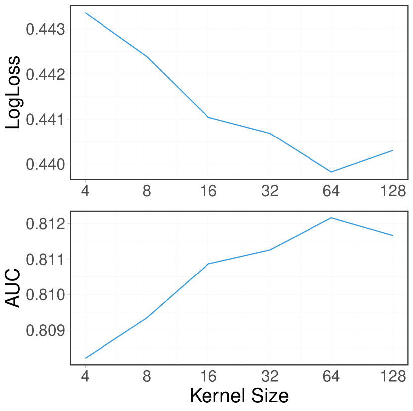
(a) Kernel Size of DynInt-DGP

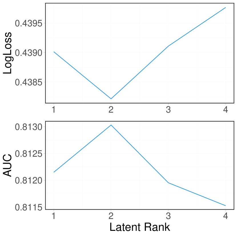
(b) Rank of DynInt-DWP

Figure 6. Logloss and AUC v.s. kernel size and latent rank.

4.4.5. Reduction Ratio

The reduction ratio is a hyper-parameter that allows us to control the capacity of our network for dynamic parameter weighting/generation. We examine the impact of reduction ratio on Criteo dataset. The correlation between the reduction ratio and performance of different architecture is similar. Other hyper-parameters maintain the same as the best setting of each specific architecture. Here we average their performance for a more straightforward illustration, as each method show a similar trend in our experiment.

7(a) shows the relationship between the different setup of reduction ratio and performance. We observe that the performance is robust to a reasonable range of reduction ratios. Increased complexity does not necessarily improve the performance, while a larger reduction ratio improves the model’s efficiency.

4.4.6. Orthogonal Regularization Rate

The orthogonal regularization rate is a hyper-parameter for controlling the representation diversity among column spaces of the dynamic parameters. Since the dynamic generated/weighting matrices can be seen as the sum of low-rank matrices, so each decomposed subspace should learn relatively distinct features. We examine the impact of orthogonal regularization rate on Criteo dataset. We average both methods’ performance for simplicity, as they show a similar trend in our experiment.

7(b) illustrates the performance v.s. the number of training steps when different orthogonal regularization ratios are applied. We observe that the orthogonal regularization improves the overall performance. We also observe that, when applied relatively larger orthogonal regularization, the overall performance is about same but larger orthogonal regularization can still improve the converge speed of the model. It indicates that encouraging the orthogonality of latent column spaces effectively improves the quality of dynamic parameter generation/weighting.

(a) Reduction Ratio

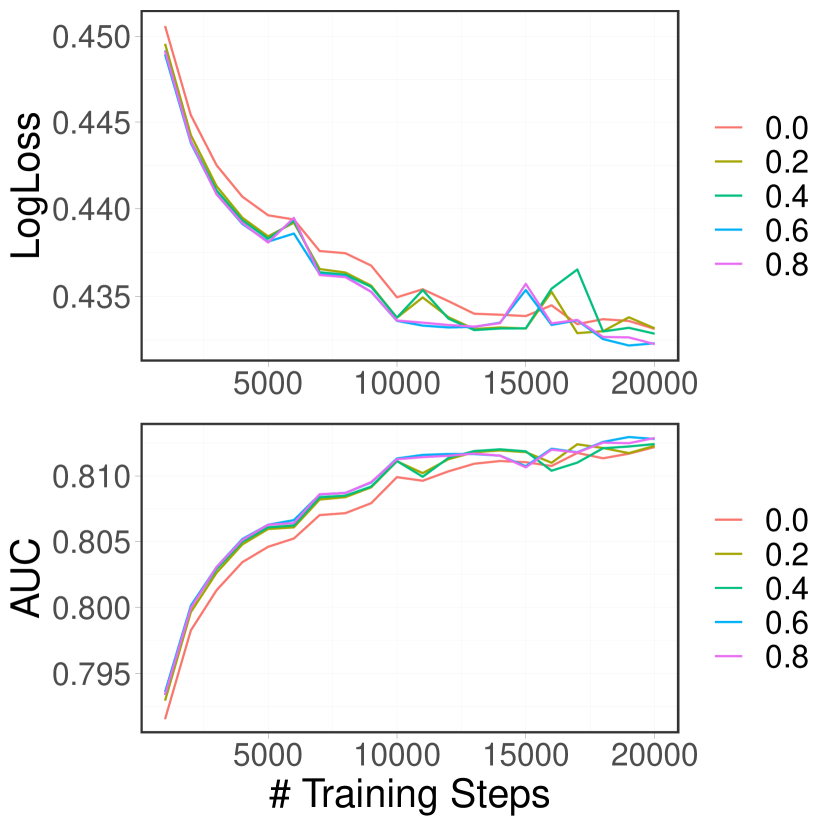
(b) Orthogonal Regularization

Figure 7. Logloss and AUC v.s. reduction ratio and orthogonal regularization rate.

5. Conclusion

Dynamic parameterization has become a popular way to leverage the deep neural networks’ representation capacity. We design our network: DynInt, with two schemes to enhance model capacity and model dynamic feature interactions. With the proposed computational paradigm based on low-rank approximation, we reduce the memory cost in implementations. Our experimental results have demonstrated its superiority over the state-of-art algorithms on real-world datasets, in terms of both model performance and efficiency.

In further work, We would like to study how to effectively and dynamically combine our model with other architectures to learn different types of interactions collectively. Beyond only modeling on fixed-length features, We also like to extend our architecture to learn on variable-length features for sequential behaviors in real-world problems.

References

- (1)
- Abadi et al. (2016) Martín Abadi, Paul Barham, Jianmin Chen, Zhifeng Chen, Andy Davis, Jeffrey Dean, Matthieu Devin, Sanjay Ghemawat, Geoffrey Irving, Michael Isard, et al. 2016. Tensorflow: A system for large-scale machine learning. In 12th USENIX Symposium on Operating Systems Design and Implementation (OSDI 16). 265–283.
- Beutel et al. (2018) Alex Beutel, Paul Covington, Sagar Jain, Can Xu, Jia Li, Vince Gatto, and Ed H Chi. 2018. Latent cross: Making use of context in recurrent recommender systems. In Proceedings of the Eleventh ACM International Conference on Web Search and Data Mining. ACM, 46–54.
- Bian et al. (2022) Weijie Bian, Kailun Wu, Lejian Ren, Qi Pi, Yujing Zhang, Can Xiao, Xiang-Rong Sheng, Yong-Nan Zhu, Zhangming Chan, Na Mou, et al. 2022. CAN: Feature Co-Action Network for Click-Through Rate Prediction. In Proceedings of the Fifteenth ACM International Conference on Web Search and Data Mining. 57–65.
- Cheng et al. (2016) Heng-Tze Cheng, Levent Koc, Jeremiah Harmsen, Tal Shaked, Tushar Chandra, Hrishi Aradhye, Glen Anderson, Greg Corrado, Wei Chai, Mustafa Ispir, et al. 2016. Wide & deep learning for recommender systems. In Proceedings of the 1st workshop on deep learning for recommender systems. ACM, 7–10.
- Dai et al. (2021) Shangfeng Dai, Haobin Lin, Zhichen Zhao, Jianying Lin, Honghuan Wu, Zhe Wang, Sen Yang, and Ji Liu. 2021. POSO: Personalized Cold Start Modules for Large-scale Recommender Systems. arXiv preprint arXiv:2108.04690 (2021).
- Dauphin et al. (2017) Yann N Dauphin, Angela Fan, Michael Auli, and David Grangier. 2017. Language modeling with gated convolutional networks. In International conference on machine learning. PMLR, 933–941.
- Guo et al. (2017) Huifeng Guo, Ruiming Tang, Yunming Ye, Zhenguo Li, and Xiuqiang He. 2017. DeepFM: a factorization-machine based neural network for CTR prediction. arXiv preprint arXiv:1703.04247 (2017).
- Ha et al. (2016) David Ha, Andrew Dai, and Quoc V Le. 2016. Hypernetworks. arXiv preprint arXiv:1609.09106 (2016).
- He et al. (2014) Xinran He, Junfeng Pan, Ou Jin, Tianbing Xu, Bo Liu, Tao Xu, Yanxin Shi, Antoine Atallah, Ralf Herbrich, Stuart Bowers, et al. 2014. Practical lessons from predicting clicks on ads at facebook. In Proceedings of the Eighth International Workshop on Data Mining for Online Advertising. ACM, 1–9.
- Hu et al. (2018) Jie Hu, Li Shen, and Gang Sun. 2018. Squeeze-and-excitation networks. In Proceedings of the IEEE conference on computer vision and pattern recognition. 7132–7141.
- Huang et al. (2020) Tongwen Huang, Qingyun She, Zhiqiang Wang, and Junlin Zhang. 2020. GateNet: gating-enhanced deep network for click-through rate prediction. arXiv preprint arXiv:2007.03519 (2020).
- Huang et al. (2019) Tongwen Huang, Zhiqi Zhang, and Junlin Zhang. 2019. FiBiNET: Combining Feature Importance and Bilinear feature Interaction for Click-Through Rate Prediction. arXiv preprint arXiv:1905.09433 (2019).
- Jia et al. (2016) Xu Jia, Bert De Brabandere, Tinne Tuytelaars, and Luc V Gool. 2016. Dynamic filter networks. Advances in neural information processing systems 29 (2016).
- Kingma and Ba (2014) Diederik P Kingma and Jimmy Ba. 2014. Adam: A method for stochastic optimization. arXiv preprint arXiv:1412.6980 (2014).
- Lian et al. (2018) Jianxun Lian, Xiaohuan Zhou, Fuzheng Zhang, Zhongxia Chen, Xing Xie, and Guangzhong Sun. 2018. xdeepfm: Combining explicit and implicit feature interactions for recommender systems. In Proceedings of the 24th ACM SIGKDD International Conference on Knowledge Discovery & Data Mining. ACM, 1754–1763.
- Ma et al. (2018) Jiaqi Ma, Zhe Zhao, Xinyang Yi, Jilin Chen, Lichan Hong, and Ed H Chi. 2018. Modeling task relationships in multi-task learning with multi-gate mixture-of-experts. In Proceedings of the 24th ACM SIGKDD International Conference on Knowledge Discovery & Data Mining. 1930–1939.
- McMahan (2011) H Brendan McMahan. 2011. Follow-the-regularized-leader and mirror descent: Equivalence theorems and l1 regularization. (2011).
- McMahan et al. (2013) H Brendan McMahan, Gary Holt, David Sculley, Michael Young, Dietmar Ebner, Julian Grady, Lan Nie, Todd Phillips, Eugene Davydov, Daniel Golovin, et al. 2013. Ad click prediction: a view from the trenches. In Proceedings of the 19th ACM SIGKDD international conference on Knowledge discovery and data mining. ACM, 1222–1230.
- Qu et al. (2016) Yanru Qu, Han Cai, Kan Ren, Weinan Zhang, Yong Yu, Ying Wen, and Jun Wang. 2016. Product-based neural networks for user response prediction. In 2016 IEEE 16th International Conference on Data Mining (ICDM). IEEE, 1149–1154.
- Qu et al. (2018) Yanru Qu, Bohui Fang, Weinan Zhang, Ruiming Tang, Minzhe Niu, Huifeng Guo, Yong Yu, and Xiuqiang He. 2018. Product-Based Neural Networks for User Response Prediction over Multi-Field Categorical Data. ACM Transactions on Information Systems (TOIS) 37, 1 (2018), 5.
- Rendle (2010) Steffen Rendle. 2010. Factorization machines. In 2010 IEEE International Conference on Data Mining. IEEE, 995–1000.
- Richardson et al. (2007) Matthew Richardson, Ewa Dominowska, and Robert Ragno. 2007. Predicting clicks: estimating the click-through rate for new ads. In Proceedings of the 16th international conference on World Wide Web. ACM, 521–530.
- Shan et al. (2016) Ying Shan, T Ryan Hoens, Jian Jiao, Haijing Wang, Dong Yu, and JC Mao. 2016. Deep crossing: Web-scale modeling without manually crafted combinatorial features. In Proceedings of the 22nd ACM SIGKDD International Conference on Knowledge Discovery and Data Mining. ACM, 255–262.
- Song et al. (2018) Weiping Song, Chence Shi, Zhiping Xiao, Zhijian Duan, Yewen Xu, Ming Zhang, and Jian Tang. 2018. AutoInt: Automatic Feature Interaction Learning via Self-Attentive Neural Networks. arXiv preprint arXiv:1810.11921 (2018).
- Swietojanski and Renals (2014) Pawel Swietojanski and Steve Renals. 2014. Learning hidden unit contributions for unsupervised speaker adaptation of neural network acoustic models. In 2014 IEEE Spoken Language Technology Workshop (SLT). IEEE, 171–176.
- Vaswani et al. (2017) Ashish Vaswani, Noam Shazeer, Niki Parmar, Jakob Uszkoreit, Llion Jones, Aidan N Gomez, Łukasz Kaiser, and Illia Polosukhin. 2017. Attention is all you need. In Advances in Neural Information Processing Systems. 5998–6008.
- Wang et al. (2017) Ruoxi Wang, Bin Fu, Gang Fu, and Mingliang Wang. 2017. Deep & cross network for ad click predictions. In Proceedings of the ADKDD’17. ACM, 12.
- Wang et al. (2021b) Ruoxi Wang, Rakesh Shivanna, Derek Cheng, Sagar Jain, Dong Lin, Lichan Hong, and Ed Chi. 2021b. DCN V2: Improved deep & cross network and practical lessons for web-scale learning to rank systems. In Proceedings of the Web Conference 2021. 1785–1797.
- Wang et al. (2021a) Zhiqiang Wang, Qingyun She, and Junlin Zhang. 2021a. MaskNet: Introducing Feature-Wise Multiplication to CTR Ranking Models by Instance-Guided Mask. arXiv preprint arXiv:2102.07619 (2021).
- Wu et al. (2019) Felix Wu, Angela Fan, Alexei Baevski, Yann N Dauphin, and Michael Auli. 2019. Pay less attention with lightweight and dynamic convolutions. arXiv preprint arXiv:1901.10430 (2019).
- Yan et al. (2022) Bencheng Yan, Pengjie Wang, Kai Zhang, Feng Li, Jian Xu, and Bo Zheng. 2022. APG: Adaptive Parameter Generation Network for Click-Through Rate Prediction. arXiv preprint arXiv:2203.16218 (2022).
- Yan and Li (2020) Yachen Yan and Liubo Li. 2020. xDeepInt: a hybrid architecture for modeling the vector-wise and bit-wise feature interactions. (2020).
- Zhang et al. (2019) Shuai Zhang, Lina Yao, Aixin Sun, and Yi Tay. 2019. Deep learning based recommender system: A survey and new perspectives. ACM Computing Surveys (CSUR) 52, 1 (2019), 5.
- Zhang et al. (2014) Weinan Zhang, Shuai Yuan, Jun Wang, and Xuehua Shen. 2014. Real-time bidding benchmarking with ipinyou dataset. arXiv preprint arXiv:1407.7073 (2014).
- Zhu et al. (2022) Yongchun Zhu, Zhenwei Tang, Yudan Liu, Fuzhen Zhuang, Ruobing Xie, Xu Zhang, Leyu Lin, and Qing He. 2022. Personalized transfer of user preferences for cross-domain recommendation. In Proceedings of the Fifteenth ACM International Conference on Web Search and Data Mining. 1507–1515.