ROTATION IN VACUUM AND SCALAR BACKGROUND:
ARE THERE ALTERNATIVES TO NEWMAN-JANIS ALGORITHM?

Abstract

The Newman-Janis algorithm is the standard approach to rotation in general relativity which, in vacuum, builds the Kerr metric from the Schwarzschild spacetime. Recently, we have shown that the same algorithm applied to the Papapetrou antiscalar spacetime produces a rotational metric devoid of horizons and ergospheres. Though exact in the scalar sector, this metric, however, satisfies the Einstein equations only asymptotically. We argue that this discrepancy between geometric and matter parts (essential only inside gravitational radius scale) is caused by the violation of the Hawking-Ellis energy conditions for the scalar energy-momentum tensor. The axial potential functions entering the metrics appear to be of the same form both in vacuum and scalar background, and they also coincide with the linearized Yang-Mills field, which might hint at their common non-gravitational origin. As an alternative to the Kerr-type spacetimes produced by Newman-Janis algorithm we suggest the exact solution obtained by local rotational coordinate transformation from the Schwarzschild spacetime. Then, comparison with the Kerr-type metrics shows that the Lense-Thirring phenomenon might be treated as a coordinate effect, similar to the Coriolis force.

PACS numbers:

1 Introduction

The Kerr solution [1] of the vacuum Einstein equations (EE) represents a mainstream approach to the rotation problems in general relativity (GR). Still, there are certain aspects about this metric which remain problematic. In spite of the variety of efforts undertaken from the outset [2], the gravitating source for the Kerr metric is still unknown [3]. Besides, absence of the interior solution, existence of closed time-like curves and the very stability of the Kerr solution are among important unresolved issues in GR [4]. In view of this, it is worthwhile to look for alternative approaches, and one of those is to consider the gravitating scalar field as realistic background instead of vacuum.

The Newman-Janis (NJ) algorithm [5] was first applied in Refs.  Krori1981 and Agnese1985 to the general static Janis-Newman-Winicour (JNW) family of solutions [8] of the EE with massless scalar field parameterized by the factor $\gamma$ related to scalar charge and taking the values within the range $[0,1]$. However, as had been recently established by the method of successive approximations [9], the result of such application of the NJ algorithm does not satisfy the Einstein-scalar equations. Meanwhile, the JNW-type spacetimes, starting with the pioneering attempt by Fisher to find the closed solution in curvature coordinates [10], are, by themselves, unstable with respect to collapse, and thus do not seem to be physically relevant [11, 12, 13, 14].

Recently, as an alternative to the JNW spacetimes, we have investigated [15] the antiscalar (i.e., having the opposite sign of the scalar field energy-momentum tensor) exponential Papapetrou solution [16] and revealed that not only it produces practically the same observational effects as in vacuum case but is also characterized by thermodynamic stability as well as the Klein-Gordon equation stability. Moreover, it leads to the value of scalar charge (the source of scalar field) being equal to the central mass [17]. Thus, the application of the NJ algorithm to the Papapetrou metric (resulting in what we call the Papapetrou-Newman-Janis metric, or PNJ for short) might be of interest. Since the exponential metric is functionally related to the JNW solution via the limit $\gamma\to\infty$ [15, 17], which falls out of the $\gamma$-range mentioned above, the problem of compatibility of the PNJ metric with the EE requires a separate study, which is one of the aims in this paper. Given that the source for the Kerr-type metrics is not established, we will also consider an alternative approach based on exact rotational solutions derived with direct coordinate transformation from the Schwarzschild metric.

2 Setup

The application of the complex-shifting NJ algorithm to the Schwarzschild metric

$$ds^{2}=(1-2M/R)dt^{2}-(1-2M/R)^{-1}{dR}^{2}-R^{2}d\Omega^{2},$$ (1)

leads to the Kerr solution (for nomenclature reasons, we also call it the Schwarzschild-Newman-Janis or SNJ metric):

$$ds^{2} = (1-2MR/\rho^{2})\left(dt-a\sin^{2}\theta d\phi\right)^{2}$$ (2)

$$- \rho^{2}\left(\frac{dR^{2}}{\Delta}+d\theta^{2}+\sin^{2}\theta d\phi^{2}\right)$$

$$+ 2a\sin^{2}\theta(dt-a\sin^{2}\theta d\phi)d\phi,$$

where $\Delta=R^{2}+a^{2}-2MR$. Note that the $g_{00}$ component contains the scalar function

$$\varphi(R,\theta,a)=MR/\rho^{2},\quad\rho^{2}(R)=R^{2}+a^{2}\cos^{2}\theta,$$ (3)

which results from complexifying the radial coordinate (see below), with the meaning of the parameter $a$ left open within the NJ algorithm.

The exponential Papapetrou metric

$$ds^{2}=e^{-2\varphi(r)}{dt}^{2}-e^{2\varphi(r)}\left({dr}^{2}+r^{2}d\Omega^{2}\right),$$ (4)

represents a static spherically symmetric solution of the general Einstein-scalar field equations

$${G}_{\mu\nu}=\epsilon\varkappa{T}_{\mu\nu}^{\text{sc}}\left(\varphi\right),$$ (5)

in antiscalar regime, i.e. with $\epsilon=-1$. Here, $\varkappa=8\pi G/c^{4}$ (we use $G=c=1$) and the minimal scalar energy-momentum tensor (EMT)

$${T}^{\text{sc}}_{\mu\nu}(\varphi)=\frac{1}{4\pi}\left(\varphi_{\mu}\varphi_{\nu}-\frac{1}{2}{g}_{\mu\nu}\varphi^{\alpha}\varphi_{\alpha}\right),\,\,\,\,\varphi_{\mu}\equiv\partial_{\mu}\varphi,$$ (6)

The values $\epsilon=0$ and $\epsilon=1$ correspond to vacuum (Schwarzschild) and scalar (JNW) solutions, correspondingly. Taking the concomitant Klein-Gordon equation into account, it follows exactly that $\varphi(r)=M/r$ for the Papapetrou metric (4).

The result of application of the NJ algorithm to the Papapetrou solution is the PNJ metric [15]:

$$ds^{2}=e^{-2\varphi(r,\theta,a)}\left(dt-a\sin^{2}\theta d\phi\right)^{2}-e^{2\varphi(r,\theta,a)}\rho^{2}\left(\frac{dr^{2}}{\underline{\Delta}}+d\theta^{2}+\sin^{2}\theta d\phi^{2}\right)\\ +2a\sin^{2}\theta(dt-a\sin^{2}\theta d\phi)d\phi.$$ (7)

This metric is similar in structure to the Kerr solution, but unlike in (2) here $\Delta\rightarrow\underline{\Delta}=r^{2}+a^{2}$, i.e. in this metric there are no horizons and ergospheres. For $a=0$ the expression (7) reduces to the Papapetrou solution (4).

The Klein-Gordon equation for the metric (7) leads to stationary rotational potential (which in this case is related to a physical scalar field) of the same functional form as in (3):

$$g^{\mu\nu}\varphi_{;\mu\nu}=0\,\,\Rightarrow\,\,\varphi=\varphi(r,\theta,a)=\frac{Mr}{\rho^{2}}=\frac{Mr}{r^{2}+a^{2}\cos^{2}\theta},$$ (8)

which in the absence of rotation ($a=0$) reduces to the Newtonian form. Note that the isotropic coordinate $r$ here should not be confused with the curvature coordinate $R$.

We use the term physical here in contrast to the Kerr, Newman-Janis and Kerr-Schild approaches where the same potential function enters into corresponding vacuum spacetime as a part of the metric coefficients after some mathematical manipulations. In our case the zero four-divergence of physical scalar EMT (6) being equivalent to the Klein-Gordon equation leads (in given coordinates) to exactly the same functional dependence for the physical background scalar field.

It is essential that final expressions (7), (8) are obtained without using the Einstein equations and so, being related directly to the scalar sector of the Lagrangian, might be considered as self-consistent. The resulting (quite cumbersome) form of the scalar EMT follows directly from substitution of (8) and (7) into (6), with the only non-zero off-diagonal components being $T_{r\theta}^{sc}$ and $T_{t\phi}^{sc}$.

3 Role of scalar background

In our approach, the expression (6) used in (5) represents a fundamental field irremovable from the field equations [15, 17], and this imposes certain constraints onto the theory as a whole, and the rotation problem in particular.

In general, the Einstein tensor and EMT, $G_{\mu\nu}$ and $\kappa T_{\mu\nu}$, are distinct objects subjected to a strict constraint in the form of the contracted Bianchi identity ${G^{\mu\nu}}_{;\nu}\equiv 0$, which represents a necessary but certainly insufficient condition for the justification of GR as a closed theory of gravitational field.

The reason for GR not being a closed theory is that the Ricci scalar $R={R^{\alpha}}_{\alpha}$ used in the Hilbert-Einstein action as geometric (‘gravitational’) part of the Lagrangian does not have the canonical (Yang-Mills-like gauge-invariant) structure quadratic with respect to first derivatives of a well-defined physical field. This circumstance leads, in particular, to such obstacle as the absence of the EMT for gravitational field itself (pseudo-tensors do not, strictly speaking, solve the problem). Taking scalar background into account may alleviate some of these problems.

At the same time, the EE prove to be an excellent tool for the description of static configurations and dynamics of homogeneous systems. In this respect note that transfer from the static metric to stationary (rotational) regime is nontrivial already in vacuum. Nontriviality follows, in particular, from the fact that it is not known in advance if the applied NJ algorithm will conserve the Ricci-flat character of the field equations.

In scalar background the problem of such transfer (generated by the NJ or some other algorithm) is much more complicated because it leads to specific transformations for both sides of the EE, which are quite different functionals with respect to metric. It is not obvious at all that coincidence of those in static cases should imply their compatibility in stationary regime as well.

The applicability of some EMT within the EE might be tested with the Hawking-Ellis (HE) approach [18] based on corresponding eigenvalue problem, i.e.

$$\left(T_{\alpha\beta}-\lambda g_{\alpha\beta}\right)V^{\beta}=0,$$ (9)

with preliminary diagonalization of the EMT via local Lorentz rotations implied, if needed. Considering the conformity with various energy dominance conditions (for more details see also Ref. VisserHE17), this approach leads to only four classification types for EMTs compatible with the EE. The predominant type I has one timelike and three spacelike eigenvectors. For contravariant components it is expressible in diagonal form,

$$T^{\alpha\beta}\sim\left(\begin{matrix}\lambda_{1}&0&0&0\\ 0&\lambda_{2}&0&0\\ 0&0&\lambda_{3}&0\\ 0&0&0&\lambda_{4}\\ \end{matrix}\right),$$ (10)

with all admissible eigenvalues $\lambda_{\mu}$ being real. We will not consider the other three types being unstable or violating some of the energy conditions.

As a matter of fact, only for definite types of metrics, when the symmetries found within the structure of the EMT are found in the Einstein tensor as well, we have meaningful integrable systems such as perfect fluids, static systems obeying time-like Killing field, homogeneous expanding universe models (a la Friedmann), and, as a degenerate case, the Ricci-flat vacuum.

In particular, as noted in Ref. galloway_topology_2021, in irrotational case, i.e. for vanishing vorticity $\omega=0$, the new symmetry conditions for $u$-congruence, $u\wedge du=0$, together with the Frobenius theorem guarantee integrability for a wide class of systems (including static scalar background) within corresponding $(1+3)$-splitting approach.

The minimal NJ method, based on linear complex shift of four-dimensional coordinates, is unique in a sense that it conserves the Ricci-flat character of equations. Indeed, in static limit the standard Kerr solution reduces to the vacuum Schwarzschild spacetime in curvature coordinates which, due to the ‘reciprocal’ condition

$$g_{00}g_{11}=-1,$$ (11)

forces the Einstein equations to be linear [3]. Exactly this linearity leads to translation invariant character of the field equations and, as an exclusive feature, to the Ricci flatness-preserving action of the NJ algorithm.

But in case of the scalar background such linearity is absent and, besides, behavior and structure of the EE in static and stationary regimes are cardinally different. It is remarkable that in the PNJ case all analytical results can be obtained exactly, and, as will be shown, the mismatch, or “splitting”, between the Einstein tensor and the scalar EMT proves to be essential only for small distances inside gravitational radius scale.

4 Stationary vs. static cases

In rotational systems the existence of additional axial Killing field, $K=\partial_{t}+\omega\partial_{\phi}$ (see Ref. mm18), leads to the conservation of energy and angular momentum, but does not guarantee the compliance with the Hawking-Ellis energy conditions. Indeed, direct substitution of the PNJ metric (7) with (8) into general relation (6) leads to the EMT non-diagonalisable by local Lorentz transformations. This violates the Hawking-Ellis condition (10), and, as a result, certain discrepancies arise between the left and right sides of the EE.

Specifically, taking the equatorial plane and designating the static case $a=0$ with solid red lines in Figs. 1(a)-1(c), the following regularities can be observed. While covariant component $T_{00}$ increases in its absolute value, $G_{00}$ decreases with the growth of rotation parameter $a$ and, simultaneously, at small distances ($r~{}\ll~{}r_{g}$) swaps the sign, which is forbidden as per energy conditions. As follows from Section 3, origin of such anomalies in behavior of $G_{\mu\nu}$ for stationary scalar background can be attributed to non-canonical character of the geometrical Lagrangian (cf. Ref. muench_brief_1998).

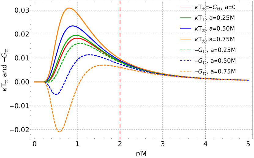
(a) Covariant components

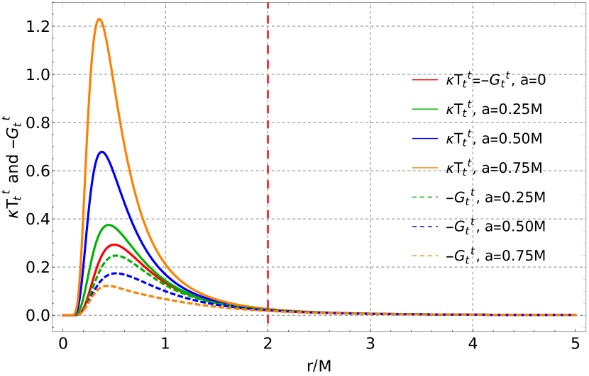
(b) Mixed components

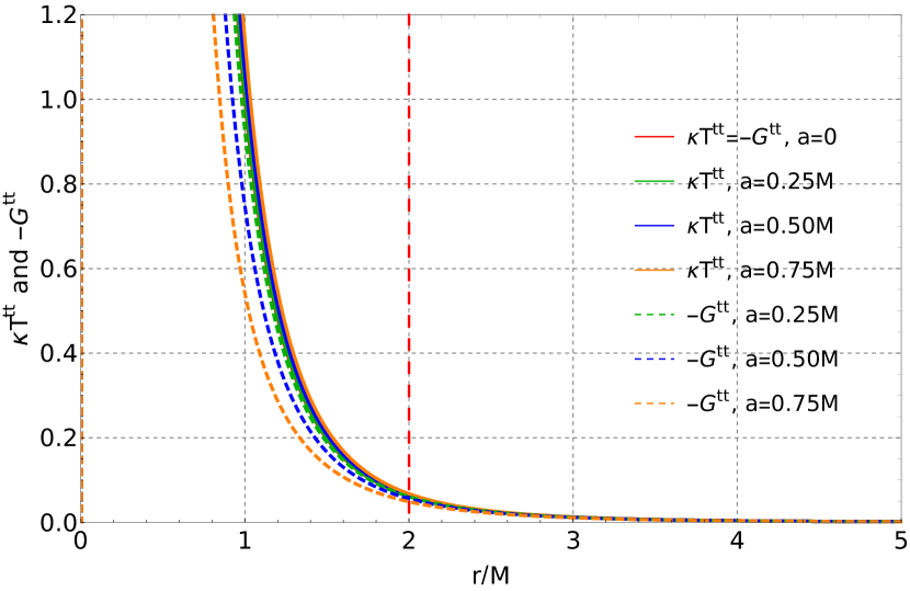
(c) Contravariant components

Figure 1: Splitting between covariant (1(a)), mixed (1(b)), and contravariant (1(c)) $tt$-components of the EMT times $\varkappa$ (solid lines) and the Einstein tensor taken with negative sign (dashed lines) for various values of $a$ in the PNJ metric, for $\theta=\pi/2$. In all cases, the curves for the Einstein tensor go below the static red line ($a=0$), and at small distances the covariant components change sign. The splitting is essential only at scales $r<r_{g}=2M$ (red dashed line).

At the same time from Fig. 1(a) one can see that for $r>r_{g}$ (as well as for small $a$) the distinction between the left and right sides in the (antiscalar) EE (5) becomes asymptotically negligible. Such asymptotic behavior might analytically be evident, in particular, from relations (33) and (32) in Appendix (A). Variation of $\theta$ does not incur essential influence on splitting effect.

Note, that only mixed components of the EMT have (for $\theta=\pi/2$) diagonal form

$${T_{\mu}}^{\nu}|_{\theta=\frac{\pi}{2}}=\frac{M^{2}\left(a^{2}+r^{2}\right)e^{-\frac{2M}{r}}}{8\pi r^{6}}\times\text{diag}(1,-1,1,1).$$ (12)

Then, as shown in Fig. 1(b), for mixed time-time component as well as for time-time component of the contravariant (non-diagonal) EMT (see Fig. 1(c)),

$$T^{tt}|_{\theta=\frac{\pi}{2}}=M^{2}\frac{a^{2}e^{-4M/r}\left(2e^{2M/r}-1\right)+r^{2}}{8\pi r^{6}}$$ (13)

with the corresponding (negative) Einstein tensor time-time components $-{G_{t}}^{t}$ and $-G^{tt}$ (not written for brevity), the splitting effect does not exhibit the peculiar behavior with the change-of-sign anomalies in the Einstein tensor. It might also be seen from Fig. 1(c) that contravariant EMT components (which enter into the HE conditions) all differ only little from the case $a=0$ which satisfies the HE conditions.

We have considered for brevity the case of $tt$-components only, but the “splitting” of the EE occurs in a similar fashion for other components as well.

5 Lense-Thirring effect for vacuum and PNJ metrics

Here we do not consider weak field approximation but deal with exact relations in strong field regime. The general frequency $\Omega$ of a test gyro in an arbitrary stationary spacetime with a timelike Killing vector $K$ can be expressed in terms of differential forms [22] as

$$\tilde{\Omega}=\frac{1}{2K^{2}}\ast\left(\tilde{K}\wedge d\tilde{K}\right),$$ (14)

where $\tilde{\Omega}$ and $\tilde{K}$ are the one-forms of $\Omega$ and $K$, and $\ast$ represents Hodge dual. The $K$ vector might be represented as a linear combination of time-translational and azimuthal vectors, $K=\partial_{t}+\omega\partial_{\phi},$ where $\omega$ is the angular velocity for an observer moving along integral curves of the $K$-field [22].

For special case $\omega=0$ the vector form of the coordinate-free general spin precession rate (14) after direct but cumbersome transformations reduces to the exact expression describing the Lense-Thirring effect (for details see, e.g., Ref. Chakraborty2017a):

$$\vec{\Omega}|_{\omega=0}=\vec{\Omega}_{LT}=\sqrt{-g_{rr}}\Omega_{LT}^{r}\hat{r}+\sqrt{-g_{\theta\theta}}\Omega_{LT}^{\theta}\hat{\theta}=\\ =\frac{1}{2\sqrt{-g}}\left[\sqrt{-g_{rr}}\left(g_{t\phi,\theta}-\frac{g_{t\phi}}{g_{tt}}g_{tt,\theta}\right)\hat{r}\right.-\left.\sqrt{-g_{\theta\theta}}\left(g_{t\phi,r}-\frac{g_{t\phi}}{g_{tt}}g_{tt,r}\right)\hat{\theta}\right].$$ (15)

In non-relativistic limit this leads to known expression for the Lense-Thirring precession [22]. The magnitude of this vector is

$$\Omega_{LT}(r,\theta)=|\vec{\Omega}_{LT}|=\sqrt{-g_{rr}(\Omega_{LT}^{r})^{2}-g_{\theta\theta}(\Omega_{LT}^{\theta})^{2}},$$ (16)

which is used in subsequent calculations. For the Kerr metric (2) this becomes [15]:

$$\Omega^{Kerr}_{LT}(R,\theta)=\frac{aM}{\rho^{3}\left(\rho^{2}-2MR\right)}\sqrt{4R^{2}\Delta\cos^{2}\theta+\left(\rho^{2}-2R^{2}\right)^{2}\sin^{2}\theta}\,\,.$$ (17)

Now, going to scalar background for the PNJ metric (7), one obtains that the vector (15) has, in accord with (16), the magnitude:

$$\Omega^{PNJ}_{LT}=\frac{ae^{-\phi(r,\theta)}}{\rho^{5}\sqrt{r^{2}+a^{2}}}\left\{\cos^{2}\theta\left[\left(1-e^{-2\phi(r,\theta)}\right)\rho^{4}+2a^{2}Mr\sin^{2}\theta\right]^{2}\right.+\\ \left.M^{2}(r^{2}+a^{2})\left(\rho^{2}-2r^{2}\right)^{2}\sin^{2}\theta\right\}^{\frac{1}{2}},$$ (18)

with $\phi(r,\theta)=Mr/\rho^{2}$ and $\rho(r,\theta)$ defined by (8).

This final relation (18) should be compared with its Kerr counterpart rewritten in “isotropic” coordinates. For that, one should substitute $R=r\left(1+\frac{M}{2r}\right)^{2}$ to get $\Omega^{Kerr}_{LT}(R,\theta)\Rightarrow\Omega^{Kerr}_{LT}(r,\theta)$. Some results of comparison of vacuum and scalar Lense-Thirring effects within $r<r_{g}=2M$ are presented in Fig. 2. For larger distances, the difference between SNJ (Kerr) and PNJ cases decreases very rapidly, as shown in Fig. 3.

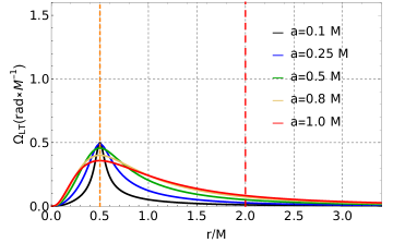
(a) vacuum (Kerr), $\theta=0$

(b) vacuum (Kerr), $\theta=\pi/2$

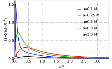
(c) scalar (PNJ), $\theta=0$

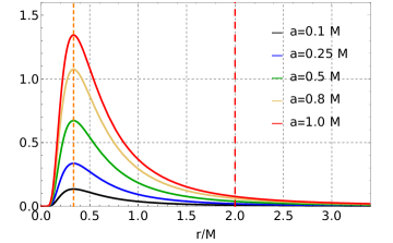
(d) scalar (PNJ), $\theta=\pi/2$

Figure 2: The Lense-Thirring precession frequency (in radians per unit time, $M$ in this case) as a function of normalized isotropic radial coordinate $r/M$, for the Kerr (top) and PNJ (bottom) metrics, for two values of the angle $\theta=0$ (left) and $\theta=\pi/2$ (right), and for five values of the parameter $a$. The precession behavior in (b) at $r/M=0.5$ is singular as opposed to the scalar counterpart where it is finite.

Due to axial symmetry planar orbits occur only for $\theta=0$ and $\theta=\pi/2$. Manipulation in inclination angle $\theta$ shows that the behavior of $\Omega^{Kerr}_{LT}$ in vacuum at $r=r_{g}/4=M/2$ becomes singular for $\theta=\pi/2$.

In contrast, in scalar background at non-zero $r$ there are no singularities in $\Omega_{LT}^{PNJ}$ which behaves monotonically and increases with the growth of $a$ arriving, for the case (d), at its maximum at $r\approx 0.32M=0.16r_{g}$ (orange vertical line) when moving in the equatorial plane $\theta=\pi/2$. At scales $r>r_{g}=2M$ the vacuum and scalar background precession effects practically coincide.

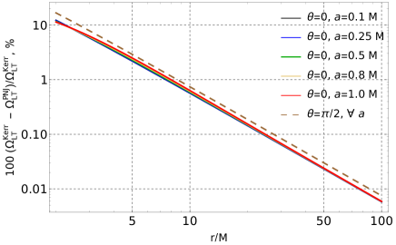
Figure 3: Relative difference in percents between Lense-Thirring frequencies $\Omega_{LT}^{Kerr}$ and $\Omega_{LT}^{PNJ}$ for larger values of $r$ (log-log scale).

6 Kerr-Schild à la Yang-Mills

The simplest complex shift by an imaginary constant $z\rightarrow z+ia$, applied to the Schwarzschild metric in Cartesian coordinates, proves to be equivalent to the NJ transformation $R^{\prime}=R+ia\cos\theta$ (see Ref. arkani-hamed_kerr_2020). Then, the Newtonian potential function entering the Schwarzschild metric transforms directly into the Kerr effective potential function, and this is a key point of the NJ approach:

$$\varphi(R)=\frac{M}{R}\quad\Rightarrow\quad\varphi(R,\theta,a)=\frac{M}{2}\left(\frac{1}{R^{\prime}}+\frac{1}{\bar{R^{\prime}}}\right)=\frac{MR}{R^{2}+a^{2}\cos^{2}\theta}.$$ (19)

These expressions coincide with those following from the bimetric Kerr-Schild form of vacuum solution [24]:

$$g_{\mu\nu}=\eta_{\mu\nu}+2\varphi k_{\mu}k_{\nu},\qquad k^{\alpha}k_{\alpha}=0,$$ (20)

with functions $\varphi=\varphi(R)$ or $\varphi=\varphi(R,\theta,a)$, correspondingly. Unlike in vacuum, in scalar background case the physical scalar fields entering the metrics (4), (7) prove to be functionally the same as in (19) but represent solutions of the Klein-Gordon equation (8).

The Kerr-Schild representation of the vacuum solutions (20) linearizes the Ricci tensor, and as a result proves to be closely related to the Yang-Mills approach in linear U(1)-invariant regime through the so-called Kerr-Schild double [23] and single [25] copy maps of Yang-Mills fields.

The indicated similarity between the gauge and gravity theories follows from correspondence between the gauge field $F_{\mu\nu}$ and the curvature tensor $R_{\mu\nu\lambda\delta}$. By analogy with self-dual Yang-Mills presentation (which admits a wave physical interpretation),

$$F_{\mu\nu}=\frac{i}{2}\epsilon_{\mu\nu\rho\sigma}F^{\rho\sigma},$$ (21)

the equations for self-dual gravity imply

$$R_{\mu\nu\lambda\delta}=\frac{i}{2}\epsilon_{\mu\nu\rho\sigma}{R^{\rho\sigma}}_{\lambda\delta}.$$ (22)

These might be analyzed in terms of the Kerr-Schild metric (cf. (20)), $g_{\mu\nu}=\eta_{\mu\nu}+2\kappa h_{\mu\nu}=\eta_{\mu\nu}+2\kappa\varphi k_{\mu}k_{\nu}$, if one includes into consideration a symbolic wave, the ‘graviton’ $h_{\mu\nu}$. The null character of $k_{\mu}$ is crucial for the linearity of the metric with respect to scalar field $\varphi$, which greatly simplifies things. Indeed, the Kerr-Schild form of the Kerr metric is chosen in analogy with the linearized presentation of the propagation of perturbed metric. However, the Kerr-Schild metric is not linearized but exact. The null character of $k_{\mu}$ allows to single out the scalar function $\phi$ which proves to be of the same functional form as the scalar field. On the other hand, exactly this function $\phi$ is related to the Yang-Mills zero component of the linearized Yang-Mills vector potential [26].

Since the vacuum Einstein equations $R_{\mu\nu}=0$ correspond, for stationary regime, to the Yang-Mills equations

$$\partial_{\mu}F^{\mu\nu}=\partial_{\mu}\left(\partial^{\mu}A^{\nu}-\partial^{\nu}A^{\mu}\right)=0,$$ (23)

the link between the gauge and Riemannian approaches might be represented via the following ansatz (see, e.g., Refs. arkani-hamed_kerr_2020,gurses2018classical,Luna):

$$A^{\mu}=\varphi k^{\mu}.$$ (24)

Then the comoving scalar potential function $\varphi$ (entering the given ansatz and calculated first in Cartesian Kerr-Schild coordinates [1]) proves to be again of familiar form (in appropriate units) [27]: $\varphi(R,\theta,a)=MR/{\rho^{2}}$, as we already indicated before, see (19) and (8).

So, the appearance of the given potential functions not only is related to but, rather, might be explained by the correspondence with non-gravitational Yang-Mills forces of nature.

Thus, the connections between the Kerr-Schild representation of the Kerr solution and stationary linear Yang-Mills fields were possible due to linear character both of the Kerr-Schild algorithm and of the corresponding Ricci-flat EE. The latter, in its turn, has origin in the linearity of the field equations in curvature coordinates (as commented in Section 4) with subsequent application of the Ricci-flatness-preserving NJ algorithm.

Importantly, in the case of scalar background, the Newman-Janis algorithm applied to isotropic exponential metric leads to physical scalar potential (8) of the same functional form as in the Kerr-Shield vacuum case which might indicate common nature.

7 Exact approach

When one applies the exact rotational coordinate transformation (hereafter, RCT)

$$\phi\to\phi-\Omega(r)t,$$ (25)

with a relevant angular velocity $\Omega(r)$ and corresponding exact differential

$$d\phi\to d\phi-\Omega(r)dt-t{\Omega}^{\prime}(r)dr,$$ (26)

to the Schwarzschild interval, one obtains an exact differentially rotating solution (hereafter, RCTS, with $S$ for Schwarzschild) as an alternative to the special algebraic Kerr (SNJ in our terms) solution, which might be used for evaluation of rotational effects. So, we get the following non-stationary representation of the Schwarzschild solution:

$$ds^{2}_{S}=N^{2}(r)dt^{2}-\psi^{4}(r)\left(dr^{2}+r^{2}d\theta^{2}+r^{2}\sin^{2}\theta(d\phi-\Omega(r)dt-t{\Omega}^{\prime}(r)dr)^{2}\right),$$ (27)

with coefficients $N(r)=Z(r)/\psi(r)$, $Z=1-\frac{M}{2r}$, $\psi=1+\frac{M}{2r}$ defined in accord with the standard Schwarzschild metric written in isotropic coordinates, or, in matrix form,

$${g}_{\mu\nu}^{S}=\psi^{4}r^{2}\sin^{2}\theta\left(\begin{array}[]{cccc}B_{S}&-t\Omega\Omega^{\prime}&0&\Omega\\ -t\Omega\Omega^{\prime}&D_{S}&0&t\Omega^{\prime}\\ 0&0&-\csc^{2}\theta&0\\ \Omega&t\Omega^{\prime}&0&-1\\ \end{array}\right),$$ (28)

where

$$B_{S}=\frac{Z^{2}}{\psi^{6}r^{2}\sin^{2}\theta}-\Omega^{2},\quad D_{S}=-\left(\frac{1}{r^{2}\sin^{2}\theta}+t^{2}\Omega^{\prime 2}\right).$$

Note that the solution (28), in general, might be satisfied with different $\Omega(r)$ (including the case  $\Omega=const$). We adopt the asymptotic condition $\Omega(r)\to 0$ when $r\to\infty$.

Then from (27)-(28) substituted into standard relations (15) and (16) one obtains, without approximations, the Lense-Thirring-type precession formula for differentially rotating frame in vacuum:

$$\Omega_{LT}^{S}=A(r,\theta)\sqrt{P^{2}(r,\theta)+(\Delta^{S}_{LT})^{2}},$$ (29)

with singular points corresponding to the zeros of the denominator of

$$A(r,\theta)=\frac{aMr\psi}{r^{4}Z^{2}\psi^{6}-4a^{2}M^{2}\sin^{2}\theta}.$$ (30)

Expanding the notation further,

$$P^{2}(r,\theta)=\sin^{2}\theta\left(\frac{12a^{2}M^{2}\sin^{2}\theta}{r^{4}\psi^{7}}+\psi\right)^{2}+4Z^{2}\cos^{2}\theta,$$

and the only non-stationary term, which is negligible if $t\Omega^{\prime}\ll 1$,

$$\Delta^{S}_{LT}=t\Omega^{\prime}Q,$$ (31)

$$Q(r,\theta)=Zr\sin{2\theta},$$

where, according to Ref. cohen67, we accept the differential rotation law:

$$\Omega(r)=\frac{2aM}{r^{3}\psi^{6}},\quad\Omega^{\prime}(r)=-\frac{6aMZ}{r^{4}\psi^{7}}=-\frac{6aM\left(1-\frac{M}{2r}\right)}{r^{4}\left(1+\frac{M}{2r}\right)^{7}}.$$

Note that (29) is stationary for $\theta=0$ and $\theta=\pi/2$, since $Q=0$ in these cases. In accord with (30), assuming $M=1$, $\theta=\pi/2$, the value of $\Omega^{S}_{LT}$ has two singular points floating (with $a$ varying from $a=0$ to $a=1$) in the interval from $r_{1}=r_{2}=r_{g}/4$ to $r_{1}=0.229$ and $r_{2}=1.091$, correspondingly. Also, $\Omega^{S}_{LT}$ changes sign between the singular points.

It is remarkable that the Lense-Thirring effects both in the Kerr case [15] and for RCTS in stationary regime for $\theta=\pi/2$, though very distinct analytically, might practically coincide (see Fig. 4). So, as a typical example, the numerical juxtaposition of (29) with the corresponding expression for the Kerr metric (reduced to isotropic-like coordinates[15]) shows that the difference is essential only at very small scales as a consequence of the initial coordinate singularity at $Z=0$.

For example, when $\theta=\pi/2$ and $a=0.25$ (blue solid line) already at $r=r_{g}$ the distinction between $\Omega_{LT}^{S}$ and $\Omega_{LT}^{Kerr}$ is $1.5\%$, for $r=3r_{g}$ it is $0.045\%$, and for $r=10r_{g}$ it is $0.00053\%$, etc., with $\Omega_{LT}^{S}$ (RCTS) values slightly prevailing over $\Omega_{LT}^{Kerr}$. Such almost negligible difference between the Kerr and RCTS effects is quite remarkable. Thus, since we are dealing with the coordinate transformation from the Schwarzschild metric, the Lense-Thirring phenomenon should be treated, similarly to that of Coriolis, as simply a coordinate effect.

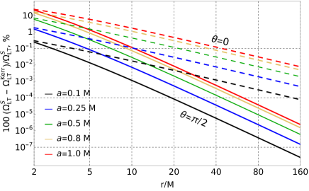
Figure 4: Relative difference in percents between Lense-Thirring frequencies $\Omega_{LT}^{S}$ and $\Omega_{LT}^{Kerr}$ for larger values of $r$ and for two values of polar angle $\theta=0$ (dashed) and $\theta=\pi/2$ (solid), in log-log scale.

For values of $\theta$ between $0$ and $\pi/2$, $\Omega_{LT}^{S}$ is non-stationary due to time-dependence of the metric, and should be studied separately.

8 Conclusion and outlook

We have analyzed the problem of application of the Newman-Janis algorithm to scalar background in general relativity in antiscalar regime, and in comparison with vacuum case.

The resulting rotational PNJ metric (7) (produced with that algorithm from the exponential Papapetrou solution (4)) contains new rotational potential. Being the solution of the Klein-Gordon equation this potential should be considered as physical. It proves to be exactly of the same form as scalar function arising in the bimetric Kerr-Schild approach in vacuum which, in its turn, coincides with the Yang-Mills potential.

This point might suggest that the Kerr spacetime (generated by the NJ algorithm) should be interpreted as a sort of pregeometry for certain (linearized) Yang-Mills fields. In such a case the PNJ metric appears as horizonless (due to presence of scalar field) counterpart of that spacetime.

The splitting between the geometric and material parts of the EE, appreciable at small radial scale, is not so unexpected because this metric makes the resulting scalar EMT incompatible with the Hawking-Ellis energy condition (10). In such case the relevant Einstein tensor exhibits anomalous structure and breaks the compatibility with scalar EMT observed in static regime.

Nevertheless, beyond the gravitational radius scale the effect of such splitting becomes negligible and practically has no impact onto distant observations. At the same time, the metric (7) by itself proves to be self-consistent and self-sufficient in the scalar sector.

The latter point deserves clarification. Indeed, as known, the variational problem based on the Ricci scalar action is not well-posed due to the necessity to fix, apart from the metric, its normal derivatives on the boundary which, in general, might be incompatible with the EE proper. This circumstance is discussed in detail in Ref. paddy22, where a radical workaround is proposed based on the application of the path integral method to the action, with subsequent exclusion of the metric from the category of dynamical variables.

A similar situation with the diminished significance of the metric also arises within GR with scalar background. Then the scalar field $\phi(x^{\mu})$ becomes in fact the only dynamical variable when the metric depends on coordinates exclusively through that field:

$$g_{\mu\nu}(x^{\mu})\,\rightarrow\,g_{\mu\nu}(\varphi(x^{\mu})).$$

So, the metric proves to be induced by scalar field and generates the final self-sufficient form of EMT producing all testable observational effects. Thus, in stationary case we get a metric emerging with the NJ algorithm inside the scalar sector, but, unlike in static case, not being an exact solution of the EE proper.

Another example of such situation indicated in Ref. paddy22 is related to the configuration with $\varphi=const$ satisfied by ${T^{\mu\nu}}_{;\nu}=0$ for massive scalar field which is not, however, a solution of the EE.

The same situation is also found in the Kaniel-Itin model [30], which contains the exponential metric, but scalar field dynamics following from the 4-divergence of the modified EMT does not comply with the EE as well.

We see that within the NJ framework one cannot also obtain the stationary rotational metric compatible both with EE proper and with the Hawking-Ellis criterion for the corresponding scalar EMT.

Then, the role of the EE proper in this case is to supply the seed exponential Papapetrou solution for subsequent generation of the horizonless scalar counterpart of the Kerr metric being only asymptotic solution of the EE and admitting also non-gravitational interpretation of its origin.

Purely gravitational variant, compatible both with the HE criterion and the EE, is developed in Section 7, based on the local rotational coordinate transformation which does not suggest introduction of any new potentials. The price for the exact solution thus obtained is, in general, its non-stationarity. At the same time, for stationary regime $\theta=\pi/2$, direct calculation and juxtaposition with the case of the Kerr metric yields practically coinciding results for the Lense-Thirring effect which allows to interpret it, similarly to that of Coriolis, as a coordinate effect, as opposed to linearized dragging and gravitomagnetic interpretations.

On the whole, apart from the HE condition, the applicability of the EE crucially depends on how exactly the rotation is introduced into spacetimes. In fact, there are only very restricted ways to do that. Here we had applied the Newman-Janis approach to scalar background, and also exact rotational transformation with respect to the vacuum Schwarzschild case as a viable alternative to Kerr. In a subsequent work, we apply another known universal Brill-Cohen method [31] based on the differential rotation ansatz, as well as relevant prolongation of the exact transformation approach to rotation in scalar background.

Appendix A $tt$-components of the EMT and Einstein tensor for the PNJ metric

In antiscalar regime, the Einstein equations (5) are $G_{\mu\nu}=-8\pi T_{\mu\nu}^{sc}$. Here, for the metric (7) specified by (8), all calculation for the left and right sides of the EE might be performed in exact form.

For example, for the covariant component of the EMT of minimal (anti)scalar field (6) one obtains:

$$8\pi T_{tt}^{sc}=\frac{M^{2}\left(a^{4}+a^{2}\left(a^{2}-3r^{2}\right)\cos{2\theta}-a^{2}r^{2}+2r^{4}\right)}{2\rho^{8}Z^{2}}.$$ (32)

At the same time the corresponding covariant $tt$-component of the Einstein tensor proves to be analytically different and much more cumbersome:

$$G_{tt}=\frac{1}{32(a^{2}+r^{2})(\rho^{2}Z)^{4}}\times\\ \Bigg{\{}3a^{6}p_{1}\cos{6\theta}+3a^{4}p_{2}\cos{4\theta}+a^{2}p_{3}\cos{2\theta}+\frac{3}{2}p_{4}+\frac{3}{4}a^{8}\cos{8\theta}\\ -2Z\Bigg{[}3a^{6}(p_{1}-2Mr)\cos{6\theta}+3a^{4}\left(p_{2}-4a^{2}Mr-8Mr^{3}\right)\cos{4\theta}+a^{2}\left(p_{3}+6a^{4}Mr\right)\cos{2\theta}\\ +\frac{3}{2}\left(p_{4}+8a^{6}Mr+16a^{4}Mr^{3}\right)+\frac{3}{4}a^{8}\cos{8\theta}\Bigg{]}\\ +Z^{2}\Bigg{[}3a^{6}(p_{1}-4Mr)\cos{6\theta}+3a^{4}\left(p_{2}-4a^{2}M^{2}-8a^{2}Mr+12M^{2}r^{2}-16Mr^{3}\right)\cos{4\theta}\\ +a^{2}\left(p_{3}-16a^{4}M^{2}+12a^{4}Mr-16a^{2}M^{2}r^{2}\right)\cos{2\theta}\\ +\frac{3}{2}\left(p_{4}-\frac{1}{3}8a^{6}M^{2}+16a^{6}Mr+8a^{4}M^{2}r^{2}+32a^{4}Mr^{3}+\frac{64}{3}a^{2}M^{2}r^{4}-\frac{64M^{2}r^{6}}{3}\right)\\ +\frac{3}{4}a^{8}\cos{8\theta}\Bigg{]}\Bigg{\}},$$ (33)

where we have used the following notations:

$$Z=e^{2\varphi(r,\theta,a)}=e^{\frac{2rM}{\rho^{2}}},\quad\rho^{2}=r^{2}+a^{2}\cos^{2}\theta,$$

$$p_{1}\left(r,a\right)=2a^{2}+3r^{2},$$

$$p_{2}\left(r,a\right)=7a^{4}+18a^{2}r^{2}+12^{4},$$

$$p_{3}\left(r,a\right)=42a^{6}+135a^{4}r^{2}+144a^{2}r^{4}+48r^{6},$$

$$p_{4}\left(r,a\right)=\frac{35}{2}a^{8}+60a^{6}r^{2}+72a^{4}r^{4}+32a^{2}r^{6}.$$

Note that apart from diagonal EMT components, there are non-zero covariant $t\phi$- and $r\theta$-components rendering the EMT non-diagonalizable with local Lorentz transformations. The same is true for the contravariant form of the EMT which thereby does not satisfy the Hawking-Ellis criterion (10).

References

- [1] R. P. Kerr, Physical Review Letters 11 (September 1963) 237.
- [2] A. Krasiński, Annals of physics 112 (1978) 22.
- [3] T. Padmanabhan, Gravitation: Foundations and Frontiers (Cambridge University Press, 2010).
- [4] L. Andersson, T. Bäckdahl, P. Blue and S. Ma, Communications in Mathematical Physics 396 (2022) 45.
- [5] E. T. Newman and A. I. Janis, Journal of Mathematical Physics 6 (1965) 915.
- [6] K. Krori and D. Bhattacharjee, Physics Letters A 82 (March 1981) 165.
- [7] A. G. Agnese and M. La Camera, Physical Review D 31 (1985) 1280.
- [8] A. I. Janis, E. T. Newman and J. Winicour, Physical Review Letters 20 (1968) 878.
- [9] I. Bogush and D. Gal’tsov, Physical Review D 102 (December 2020) 124006.
- [10] I. Z. Fisher, Zhurnal Experimental’noj i Teoreticheskoj Fiziki 18 (November 1948) 636, arXiv: gr-qc/9911008.
- [11] S. Abe, Physical Review D 38 (1988) 1053.
- [12] D. Christodoulou, Annals of Mathematics 149 (1999) 183.
- [13] J. Liu and J. Li, Communications in Mathematical Physics 363 (2018) 561.
- [14] V. Faraoni, A. Giusti and B. H. Fahim, Physics Reports 925 (2021) 1.
- [15] M. A. Makukov and E. G. Mychelkin, Physical Review D 98 (September 2018) 064050, arXiv: 1809.05290.
- [16] A. Papapetrou, Zeitschrift für Physik A 139 (1954) 518.
- [17] M. Makukov and E. Mychelkin, Foundations of Physics 50 (2020) 1346.
- [18] S. W. Hawking and G. F. R. Ellis, The Large Scale Structure of Space-time (Cambridge University Press, Cambridge, 1973).
- [19] P. Martín-Moruno and M. Visser, Classical and semi-classical energy conditions, in Wormholes, Warp Drives and Energy Conditions, ed. F. S. N. Lobo (Springer International Publishing, Cham, 2017), Cham, pp. 193–213. arXiv: 1702.05915.
- [20] G. J. Galloway, M. A. Khuri and E. Woolgar, Classical and Quantum Gravity 39 (2022) 195004.
- [21] U. Muench, F. Gronwald and F. W. Hehl, General Relativity and Gravitation 30 (June 1998) 933.
- [22] C. Chakraborty, P. Kocherlakota, M. Patil, S. Bhattacharyya, P. S. Joshi and A. Królak, Physical Review D 95 (2017) 1, arXiv: 1611.08808.
- [23] N. Arkani-Hamed, Y.-t. Huang and D. O’Connell, Journal of High Energy Physics 2020 (January 2020) 46.
- [24] R. P. Kerr and A. Schild, General Relativity and Gravitation 41 (October 2009) 2485.
- [25] R. Alawadhi, D. S. Berman, C. D. White and S. Wikeley, Journal of High Energy Physics 2021 (2021) 1.
- [26] M. Gürses and B. Tekin, Physical Review D 98 (2018) 126017.
- [27] A. Luna Godoy, The double copy and classical solutions, PhD thesis, University of Glasgow (2018).
- [28] J. M. Cohen, Journal of Mathematical Physics 8 (July 1967) 1477, Publisher: American Institute of Physics.
- [29] T. Padmanabhan and S. Chakraborty, Physics Letters B 824 (January 2022) 136828, arXiv: 2112.09446.
- [30] U. Muench, F. Gronwald and F. W. Hehl, General Relativity and Gravitation 30 (June 1998) 933.
- [31] D. R. Brill and J. M. Cohen, Physical Review 143 (1966) 1011.