Enhancing Deep Learning with Scenario-Based
Override Rules: a Case Study

Abstract

Deep neural networks (DNNs) have become a crucial instrument in the software development toolkit, due to their ability to efficiently solve complex problems. Nevertheless, DNNs are highly opaque, and can behave in an unexpected manner when they encounter unfamiliar input. One promising approach for addressing this challenge is by extending DNN-based systems with hand-crafted override rules, which override the DNN’s output when certain conditions are met. Here, we advocate crafting such override rules using the well-studied scenario-based modeling paradigm, which produces rules that are simple, extensible, and powerful enough to ensure the safety of the DNN, while also rendering the system more translucent. We report on two extensive case studies, which demonstrate the feasibility of the approach; and through them, propose an extension to scenario-based modeling, which facilitates its integration with DNN components. We regard this work as a step towards creating safer and more reliable DNN-based systems and models.

1 INTRODUCTION

Deep learning (DL) algorithms have been revolutionizing the world of Computer Science, by enabling engineers to automatically generate software systems that achieve excellent performance [Goodfellow et al., 2016]. DL algorithms can generalize examples of the desired behavior of a system into an artifact called a deep neural network (DNN), whose performance often exceeds that of manually designed software [Simonyan and Zisserman, 2014, Silver et al., 2016]. DNNs are now being extensively used in domains such as game playing [Mnih et al., 2013], natural language processing [Collobert et al., 2011], protein folding [Jumper et al., 2021], and many others. In addition, they are also being used as controllers within critical reactive systems, such as autonomous cars and unmanned aircraft [Bojarski et al., 2016, Julian et al., 2016].

Although systems powered by DNNs have achieved unprecedented results, there is still room for improvement. DNNs are trained automatically, and are highly opaque — meaning that we do not comprehend, and cannot reason about, their decision-making process. This inability is a cause for concern, as DNNs do not always generalize well, and can make severe mistakes. For example, it has been observed that state-of-the-art DNNs for traffic sign recognition can misclassify “stop” signs, even though they have been trained on millions of street images [Papernot et al., 2017]. When DNNs are deployed in reactive systems that are safety critical, such mistakes could potentially endanger human lives. It is therefore necessary to enhance the safety and dependability of these systems, prior to their deployment in the field.

One appealing approach for bridging the gap between the high performance of DNNs and the required level of reliability is to guard DNNs with additional, hand-crafted components, which could override the DNNs in case of clear mistakes [Shalev-Shwartz et al., 2016, Avni et al., 2019]. This, in turn, raises the question of how to design and implement these guard components. More recent work [Harel et al., 2022, Katz, 2021a, Katz, 2020] has suggested fusing DL with modern software engineering (SE) paradigms, in a way that would allow for improving the development process, user experience, and overall safety of the resulting systems. The idea is to enable domain experts to efficiently and conveniently pour their knowledge into the system, in the form of hand-crafted modules that will guarantee that unexpected behavior is avoided.

Here, we focus on one particular mechanism for producing such guard rules, through the scenario-based modeling (SBM) paradigm [Harel et al., 2012]. SBM is a software development paradigm, whose goal is to enable users to model systems in a way that is aligned with how they are perceived by humans [Gordon et al., 2012]. In SBM, the user specifies scenarios, each of which represents a single desirable or undesirable system behavior. These scenarios are fully executable, and can be interleaved together at runtime in order to produce cohesive system behavior. Various studies have shown that SBM is particularly suited for modeling reactive systems [Bar-Sinai et al., 2018a]; and in particular, reactive systems that involve DNN components [Yerushalmi et al., 2022, Corsi et al., 2022a].

The research questions that we tackled in this work are:

1. Can the approach of integrating SBM and DL be applied to state-of-the-art deep learning projects?

2. Are there idioms that, if added to SBM, could facilitate this integration?

To answer these questions, we apply SBM to guard two reactive systems powered by deep learning: (1) Aurora [Jay et al., 2019], a congestion control protocol whose goal is to optimize the communication throughput of a computer network; and (2) the Turtlebot3 platform [Nandkumar et al., 2021], a mobile robot capable of performing mapless navigation towards a predefined target through the use of a pre-trained DNN as its policy. In both cases, we instrument the DNN core of the system with an SBM harness; and then introduce guard scenarios for overriding the DNN’s outputs in various undesirable situations. In both case studies, we demonstrate that our SBM components can indeed enforce various safety goals. The answer to our first research question is therefore positive, since these initial results demonstrate the applicability and usefulness of this approach.

As part of our work on the Aurora and Turtlebot3 systems, we observed that the integration between the underlying DNNs and SBM components was not always straightforward. One recurring challenge, which the SBM framework could only partially tackle, was the need for the SB model to react immediately, in the same time step, to the decisions made by the DNN — as opposed to only reacting to actions that occurred in previous time steps [Harel et al., 2012]. This issue could be circumvented, but this entailed using ad hoc solutions that go against the grain of SBM. This observation answers our second research question: indeed, certain enhancements to SBM are necessary to facilitate a more seamless combination of SBM and DL. In order to overcome this difficulty in a more principled way, we propose here an extension to the SBM framework with a new type of scenario, which we refer to as a modifier scenario. This extension enabled us to create a cleaner and more maintainable scenario-based model to guard the DNNs in question. We describe the experience of using the new kind of scenario, and provide a formal extension to SBM that includes it.

The rest of the paper is organized as follows. In Sec. 2 we provide the necessary background on DNNs, and their guarding using SBM. In Sec. 3 and Sec. 4 we describe our two case studies. Next, in Sec. 5 we present our extension to SBM, which supports modifier scenarios. We follow with a discussion of related work in Sec. 6, and conclude in Sec. 7.

2 BACKGROUND

2.1 Deep Reinforcement Learning

At a high level, a neural network $N$ can be regarded as a transformation that maps an input vector $x$ into an output vector $N(x)$. For example, the small network depicted in Fig. 1 has an input layer, a single hidden layer, and an output layer. After the input nodes are assigned values by the user, the assignment of each consecutive layer’s nodes is computed iteratively, as a weighted sum of neurons from its preceding layer, followed by an activation function. For the network in Fig. 1, the activation function in use is $y=\text{ReLU}{}(x)=\max(0,x)$ [Nair and Hinton, 2010]. For example, for an input vector $x=(x_{1},x_{2})$, and an assignment $x_{1}=1,x_{2}=0$, this process results in the output neurons being assigned the values $y_{1}=0,y_{2}=2$, and $N(x)=(y_{1},y_{2})$. If the network acts as a classifier, we slightly abuse notation and associate each label with the corresponding output neuron. In this case, since $y_{2}$ has the higher score, input $x=(1,0)$ is classified as the label $y_{2}$. For additional background on DNNs, see, e.g., [Goodfellow et al., 2016].

Figure 1: A small neural network. In orange: the values computed for each neuron, for input $(1,0)$.

One method for producing DNNs is via deep reinforcement learning (DRL) [Sutton and Barto, 2018]. In DRL, an agent is trained to interact with an environment. Each time, the agent selects an action, with the goal of maximizing a predetermined reward function. The process can be regarded as a Markov decision process (MDP), where the agent attempts to learn a policy for maximizing its returns. DRL algorithms are used to train DNNs to learn optimal policies, through trial and error. DRL has shown excellent results in the context of video games, robotics, and in various safety-critical systems such as autonomous driving and flight control [Sutton and Barto, 2018].

Fig. 2 describes the basic interaction between a DRL agent and its environment. At time step $t$, the agent examines the environment’s state $s_{t}$, and chooses an action $a_{t}$ according to its current policy. At time step ${t+1}$, and following the selected action $a_{t}$, the agent receives a reward $R_{t}=R(s_{t},a_{t})$. The environment then shifts to state $s_{t+1}$ where the process is repeated. A DRL algorithm trains a DNN to learn an optimal policy for this interaction.

Figure 2: The agent-environment interaction in reinforcement learning (borrowed from [Sutton and Barto, 2018]).

2.2 Override Rules

Given a DNN $N$, an override rule [Katz, 2020] is defined as a triple $\langle P,Q,\alpha\rangle$, where:

• $P$ is a predicate over the network’s input $x$.

• $Q$ is a predicate over the network’s output $N(x)$.

• $\alpha$ is an override action.

The semantics of an override rule is that if $P(x)$ and $Q(N(x))$ evaluate to True for the current input $x$ and the network calculation $N(x)$, then the output action $\alpha$ should be selected — notwithstanding of the network’s output. For example, for the network from Fig. 1, we might define the following rule:

$$\langle x_{1}>x_{2},\text{True}{},y_{1}\rangle$$

We previously saw that for inputs $x_{1}=1,x_{2}=0$, the network selects the label corresponding to $y_{2}$. However, if we enforce this override rule, the selection will be modified to $y_{1}$. This is because this particular input satisfies the rule’s conditions (note that $Q=\text{True}{}$ means that there are no restrictions on the DNN’s output). By adjusting $P$ and $Q$, this formulation can express a large variety of rules [Katz, 2020].

2.3 Scenario-Based Modeling

Scenario-based modeling (SBM) [Harel et al., 2012], also known as behavioral programming (BP), is a paradigm for modeling complex reactive systems. The approach is focused on enabling users to naturally model their perception of the system’s requirements [Gordon et al., 2012]. At the center of this approach lies the concept of a scenario object: a depiction of a single behavior, either desirable or undesirable, of the system being modeled. Each scenario object is created separately, and has no direct contact with the other scenarios. Rather, it communicates with a global execution mechanism, which can execute a set of scenarios in a manner that produces cohesive global behavior.

More specifically, a scenario object can be viewed as a transition system, whose states are referred to as synchronization points. When the scenario reaches a synchronization point, it suspends and declares which events it would like to trigger (requested events), which events are forbidden from its perspective (blocked events), and which events it does not explicitly request, but would like to be notified should they be triggered (waited-for events). The execution infrastructure waits for all the scenarios to synchronize (or for a subset thereof [Harel et al., 2013]), and selects an event that is requested and not blocked for triggering. The mechanism then notifies the scenarios requesting/waiting-for this event that it has been triggered. The notified scenarios proceed with their execution until reaching the next synchronization point, where the process is repeated.

A toy example of a scenario-based model appears in Fig. 3. This model is designed to control a Robotis Turtlebot 3 platform (Turtlebot, for short) [Nandkumar et al., 2021, Amsters and Slaets, 2019]. The robot’s goal is to perform mapless navigation towards a predefined target, using information from lidar sensors and information about the current angle and distance from the target. The scenarios are described as transition systems, where nodes represent synchronization points. The MoveForward scenario waits for the InputEvent event, which includes a payload vector, $v_{t}$, that contains sensor readings. If $v_{t}$ indicates that the area directly in front of the robot is clear, the scenario requests the event Forward. Clearly, in many cases moving forward is insufficient for solving a maze, and so we introduce a second scenario, TurnLeft. This scenario waits for an InputEvent event with a payload vector $v_{t}$ indicating that the area to the left of the robot is clear. It then requests the Left event. Further, the TurnLeft scenario blocks the Forward event, to make the robot prefer a left turn to a move forward (inspired by the left-hand rule [Contributors, 2022b]). Finally, The MoveForward scenario waits for the event Left, to return to its initial state even if the Forward event was not triggered.

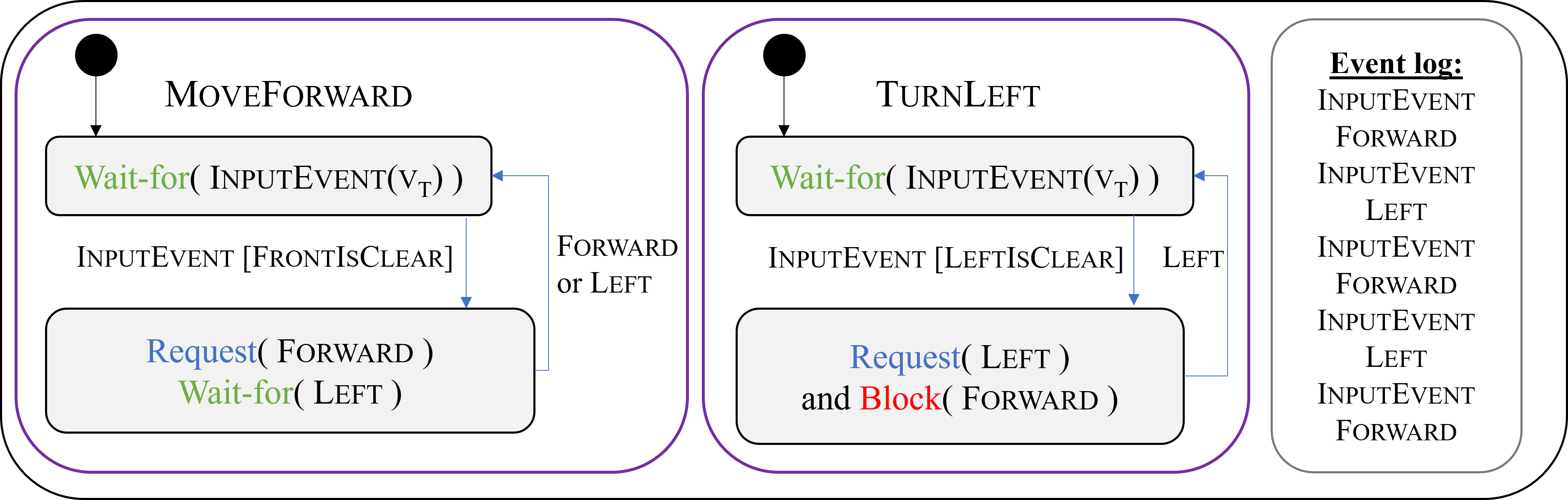
Figure 3: On the left, a screenshot of the Turtlebot simulator, where the robot is headed right and the target appears in the top left corner. In the middle, the scenario-based model, written in Statechart-like transition systems [Harel, 1986] extended with SBM. The model contains two scenarios: The MoveForward scenario and the TurnLeft scenario. The black circles specify the initial state. In each state the scenario can request, wait-for or block events. Once a requested/waited-for event is triggered, the scenario transitions to the appropriate state (highlighted by a connecting edge with the event name and an optional Boolean condition). On the right, a log of the triggered events during the execution, for this particular maze.

The SBM paradigm is well established, and has been studied thoroughly in the past years. It has been implemented on top of Java [Harel et al., 2010], JavaScript [Bar-Sinai et al., 2018b], ScenarioTools, C++ [Harel and Katz, 2014], and Python [Yaacov, 2020]; and has been used to model various complex systems, such as cache coherence protocols, robotic controllers, games, and more [Harel et al., 2016, Ashrov et al., 2015, Harel et al., 2018]. A key advantage of SBM is that its models can be checked and formally verified [Harel et al., 2015b], and that automatic tools can be applied to repair and launch SBM in distributed environments [Steinberg et al., 2018, Harel et al., 2014, Harel et al., 2015a].

In formalizing SBM, we follow the definitions of Katz [Katz, 2013]. A scenario object $O$ over a given event set $E$ is abstractly defined as a tuple $O=\langle Q,q_{0},\delta,R,B\rangle$, where:

• $Q$ is a set of states, each representing one of the predetermined synchronization points.

• $q_{0}\in Q$ is the initial state.

• $R:Q\to 2^{E}$ and $B:Q\to 2^{E}$ map states to the sets of events requested or blocked at these states (respectively).

• $\delta:Q\times E\to Q$ is a deterministic transition function, indicating how the scenario reacts when an event is triggered.

Let $M=\{O^{1},...,O^{n}\}$ be a be a behavioral model, where $n\in N$ and each $O^{i}=\langle Q^{i},q_{0}^{i},\delta^{i},R^{i},B^{i}\rangle$ is a distinct scenario. In order to define the semantics of $M$, we construct a deterministic labeled transition system $LTS(M)=\langle Q,q_{0},\delta\rangle$, where:

• $Q:=Q^{1}\times...\times Q^{n}$ is the set of states.

• $q_{0}:=\langle q_{0}^{1},...,q_{0}^{n}\rangle\in Q$ is the initial state.

• $\delta:Q\times E\to Q$ is a deterministic transition function, defined for all $q=\langle q^{1},...,q^{n}\rangle\in Q$ and $e\in E$, by:

$$\delta(q,e):=\langle\delta^{1}(q^{1},e),...,\delta^{n}(q^{n},e)\rangle$$

An execution of $M$ is an execution of the induced $\text{LTS}{}(M)$. The execution starts at the initial state $q_{0}$. In each state $q=\langle q^{1},\ldots,q^{n}\rangle\in Q$, the event selection mechanism (ESM) inspects the set of enabled events $E(q)$ defined by:

$$E(q):=\bigcup\limits_{i=1}^{n}R^{i}(q^{i})\setminus\bigcup\limits_{i=1}^{n}B^{i}(q^{i})$$

If $E(q)\neq\emptyset$, the mechanism selects an event $e\in E(q)$ (which is requested and not blocked). Event $e$ is then triggered, and the system moves to the next state, $q^{\prime}=\delta(q,e)$, where the execution continues. An execution can be formally recorded as a sequence of triggered events, called a run. The set of all complete runs is denoted by $\mathcal{L}(M)\triangleq\mathcal{L}(\text{LTS}{}(M))$. It contains both infinite runs, and finite runs that end in terminal states, i.e. states in which there are no enabled events.

2.4 Modeling Override Scenarios using SBM

We follow a recently proposed method [Katz, 2020, Katz, 2021a] for designing SBM models that integrate scenario objects and a DNN controller. The main concept is to represent the DNN as a scenario object, $O_{DNN}$, that operates as part of the scenario-based model, enabling the different scenarios to interact with the DNN. As a first step, we assume that there is a finite set of possible inputs to the DNN, denoted $\mathbb{I}$; and let $\mathbb{O}$ mark the set of possible actions the DNN can select from (we relax the limitation of finite event sets later on). We add new events to the event set $E$: an event $e_{i}$ that contains a payload of the input values for every $i\in\mathbb{I}$, and an event $e_{o}$ for every $o\in\mathbb{O}$. The scenario object $O_{DNN}$ continually waits for all events $e_{i}$, and then requests all output events $e_{o}$. This modeled behavior captures the black-box nature of the DNN: after an input arrives, one of the possible outputs is chosen, but we do not know which. However, when the model is deployed, the execution infrastructure evaluates the actual DNN, and triggers the event that it selects. For instance, assuming that there are only two possible inputs: $i_{1}=\langle 1,0\rangle$ and $i_{2}=\langle 0,1\rangle$, the network portrayed in Fig. 1 would be represented by the scenario object depicted in Fig. 4.

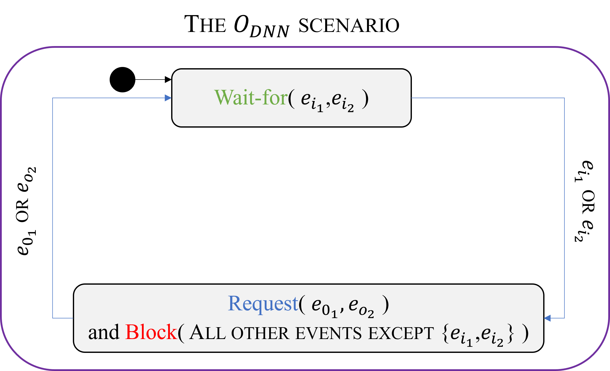
Figure 4: A figure of the $O_{DNN}$ scenario object corresponding to the neural network in Fig. 1 described in statecharts. The black circle indicates the initial state. The scenario waits for the events $e_{i_{1}}$ and $e_{i_{2}}$ that represent the inputs to the neural network. These events contain a payload with the actual values assigned. The scenario then proceeds to request the events $e_{o_{1}}$ and $e_{o_{2}}$, which represent the possible output labels $y_{1},y_{2}$ respectively (inspired by [Katz, 2021a]).

By convention, we stipulate that scenario objects in the system may wait-for the input events $e_{i}$, but may not block them. A dedicated scenario object, the sensor, is in charge of requesting an input event when the DNN needs to be evaluated. Another convention is that only the $O_{DNN}$ may request the output events, $e_{o}$; although other scenarios may wait-for or block these events. At run time, if the DNN’s classification result is an event which is currently blocked, the event selection mechanism resolves this by selecting a different output event which is not blocked. If there are no unblocked events, the system is considered deadlocked, and the SBM program terminates. The motivation for these conventions is to allow scenario objects to monitor the DNN’s inputs and outputs. The scenarios can then intervene, and override the DNN’s output — by blocking specific output events. An override scenario can coerce the DNN to select a specific output, by blocking all other output events; or it can interfere in a more subtle manner, by blocking some output events, while allowing $O_{DNN}$ to select from the remaining ones. One strategy for selecting an alternate output event in a classification problem will be to select the event with the next-to-highest score.

In practice, the requirement that the event sets $\mathbb{I}$ and $\mathbb{O}$ be finite is restrictive, as DNNs typically have a very large (effectively infinite) number of possible inputs. To overcome this restriction, we follow the extension proposed in [Katz et al., 2019], which enables us to treat events as typed variables, or sets thereof. Using this extension, the various scenarios can affect, through requesting and blocking, the possible values of these variables; and a scenario object’s transitions may be conditioned upon the values of these variables. In particular, these variables can be used to express an infinite number of possible inputs and outputs of a DNN.

Using the aforementioned extension, the override rule from Sec. 2.1 is depicted in Fig. 5. The scenario waits for the input event $e_{i}$, which now contains as a payload two real-valued variables, $x_{1}$ and $x_{2}$, that represent the actual assignment to the DNN’s inputs. The transitions of the scenario object are then conditioned upon the values of these variables: if the predicate $P$ holds for this input, the scenario transitions to its second state, where it overrides the DNN’s output by blocking the output event $e_{y_{2}}$, which necessarily causes the triggering of $e_{y_{1}}$.

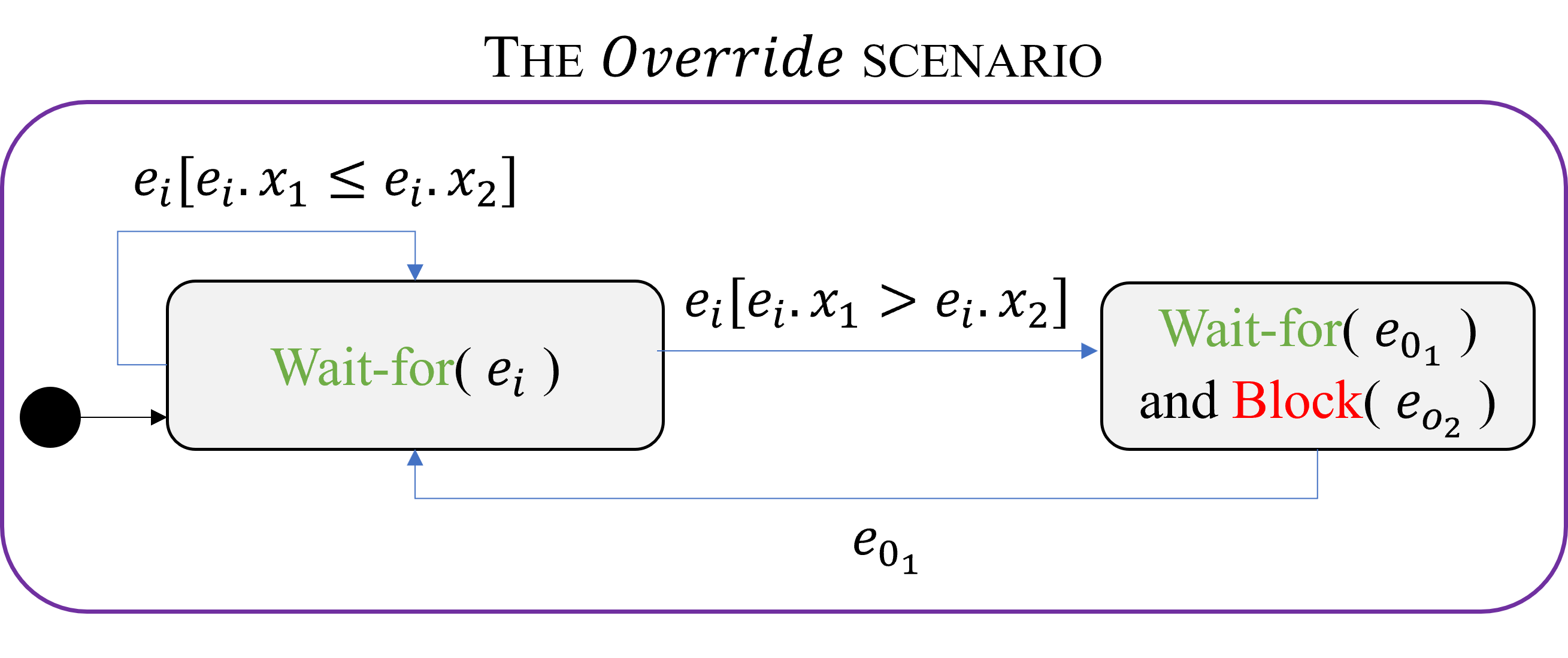
Figure 5: A scenario object for enforcing the override rule defined in Sec. 2.2. The scenario waits for the input event $e_{i}$ and inspects the payload to see if the predicate $P$ holds for the given input. It then continues to wait for the output event $e_{o_{1}}$, while blocking the unwanted event $e_{o_{2}}$. This blocking forces the triggering of output event $e_{o_{1}}$. Once this happens, the scenario returns to its initial state.

3 CASE STUDY: THE AURORA CONGESTION CONTROLLER

For our first case study, we focus on Aurora [Jay et al., 2019] — a recently proposed performance-oriented congestion control (PCC) protocol, whose purpose is to manage a computer network (e.g., the Internet). Aurora’s goal is to maximize the network’s throughput, and to prevent “congestive collapses”, i.e., situations where the incoming traffic rate exceeds the outgoing bandwidth and packets are lost. Aurora is powered by a DRL-trained DNN agent that attempts to learn an optimal policy with respect to the environment’s state and reward, which reflect the agent’s performance in previous batches of sent packets. The action selected by the agent is the sending rate that is used for the next batch of packets. It has been shown that Aurora can obtain impressive results, competitive with modern, hand-crafted algorithms for similar purposes [Jay et al., 2019].

Aurora employs the concept of monitor intervals (MIs) [Dong et al., 2018], in which time is split into consecutive intervals. At the start of each MI, the agent’s chosen action $a_{t}$ (a real value) is selected as the sending rate for the current MI, and it remains fixed throughout the interval. This rate affects the pace, and eventually the throughput, of the protocol. After the MI has finished, a vector $v_{t}$ containing real-valued performance statistics is computed from data collected during the interval. Subsequently, $v_{t}$ is provided as the environment state to the agent, which then proceeds to select a new sending rate $a_{t+1}$ for the next MI, and so on. For a more extensive background on performance-oriented congestion control, see [Dong et al., 2015].

As a supporting tool, Aurora is distributed with the PCC-DL simulator [Meng et al., 2020a] that enables the user to test Aurora’s performance. The simulator has two built-in congestion control protocols:

• The PCC-IXP protocol: a simple protocol that adjusts the sending rate using a hard-coded function.

• The PCC-Python protocol: a protocol that utilizes a trained Aurora agent to adjust the sending rate.

Both of these protocols are classified as normal (primary) protocols that aspire to maximize their throughput [Meng et al., 2020b].

We chose Aurora as our first case study because of its reactive nature: it receives external input from the environment, processes this information using the trained DRL agent, and acts on it with the next sending rate. SBM is well suited for reactive systems [Harel et al., 2012], and Aurora matched our requirements to enhance a reactive DL system. The goals we set out to achieve in this case study are detailed in the following section.

3.1 Integrating Aurora and SBM

Our first goal was to instrument the Aurora DNN agent with the $O_{DNN}$ infrastructure, and integrate it with an SB model. This was achieved through the inclusion of the C++ SBM package [Harel and Katz, 2014, Katz, 2021b] in the simulator; and the introduction of a new protocol, PCC-SBM, which extends the PCC-Python protocol and launches an SB model that includes the $O_{DNN}$ scenario. This process, on which we elaborate next, required significant technical work — and successfully produced an integrated SBM/DNN model that performed on par with the original, DNN-based model.

The simulator interacts with the PCC-SBM protocol in two ways: (i) it provides the statistics of the current MI; and (ii) it requests the next sending rate. Thus, we began the SBM/DNN integration by introducing a Sensor scenario, whose purpose is to inject MonitorInterval and QueryNextSendingRate events into the SB model, to allow it to communicate with the simulator. Fig. 6 depicts the Aurora $O_{DNN}$ scenario (using a combination of Statecharts and SBM visual languages [Harel, 1986, Marron et al., 2018]), which waits for these events in its initial state. The event MonitorInterval carries, as a payload, the MI statistics vector, $v_{t}$, whose entries are real values.

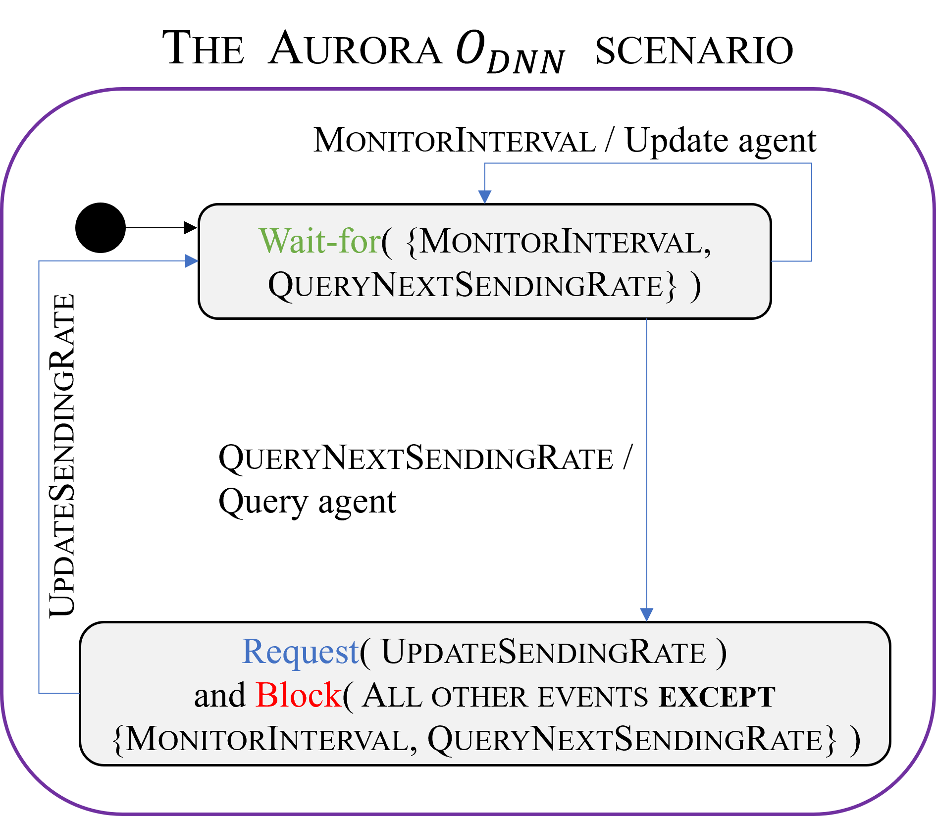
Figure 6: The Aurora $O_{DNN}$ scenario.

When MonitorInterval is triggered, the statistics vector is provided as the input to the underlying DNN, and when the event QueryNextSendingRate is triggered, the scenario extracts the DNN’s output, and then uses it as a payload for an UpdateSendingRate that it requests — while blocking all other, non-input events. Finally, we introduce an Actuator scenario, which waits for the event UpdateSendingRate and updates the simulator on the selected sending rate for the next batch of packets.

3.2 Supporting Scavenger Mode

For our second, more ambitious goal, we set out to extend the Aurora system with a new behavior, without altering its underlying DNN: specifically, with the ability to support scavenger mode [Meng et al., 2020b]. The scavenger protocol is a “polite” protocol, meaning it can yield its throughput if there is competition in the same physical network. Of course, such behavior needs to be temporary, and when the other traffic on the physical network subsides, the scavenger protocol should again increase its throughput, utilizing as much of the available bandwidth as possible.

In order to add scavenger mode support, we added the following scenarios:

• The MonitorNetworkState scenario object, which inspects the state of the physical network and requests a specific event: the EnterYield event that marks that the conditions for entering yield mode, in which sending rates should be reduced, are met.

• The ReduceThroughput scenario object, which is an override scenario. This scenario first waits-for a notification that the protocol should enter yield mode, and then proceeds to override the DNN’s calculated sending rate with a lower sending rate.

Our plan was for the ReduceThroughput scenario to support three override policies: (i) an immediate decline to a fixed, low sending rate; (ii) a gradual decline, using a step function; and (iii) a gradual decline, using exponential decay. However, we quickly observed that the existing override scenario formulation (as presented in Sec. 2.4) was not suitable for this task.

Recall that an override scenario overrides $O_{DNN}$’s output by blocking any unwanted output events, and coercing the event selection mechanism to select a different output event that is not blocked. In our case, however, we needed ReduceThroughput to act as an override scenario that blocks some output events based on the output selected by $O_{DNN}$, in the current time step. For example, in the case of a gradual decline in the sending rate, if $O_{DNN}$ would normally select sending rate $x$, we might want to force the selection of rate $\frac{x}{2}$, instead; but this requires knowing the value of $x$, in advance, which is simply not possible using the current formulation [Katz, 2020].

To circumvent this issue within the existing modeling framework, we introduce a new “proxy event”, UpdateSendingRateReduce, intended to serve as a middleman between the Aurora $O_{DNN}$ scenario and its consumers. Our override scenario, ReduceThroughput, no longer directly blocks certain values that the DNN might produce. Instead, it waits-for the UpdateSendingRate event produced by Aurora $O_{DNN}$, manipulates its real-valued payload as needed, and then requests the proxy event UpdateSendingRateReduce with the (possibly) modified value. Then, in every scenario that originally waited-for the UpdateSendingRate event, we rename the event to UpdateSendingRateReduce, so that the scenario now waits for the proxy event, instead. Fig. 7 visually illustrates the final version of the ReduceThroughput scenario.

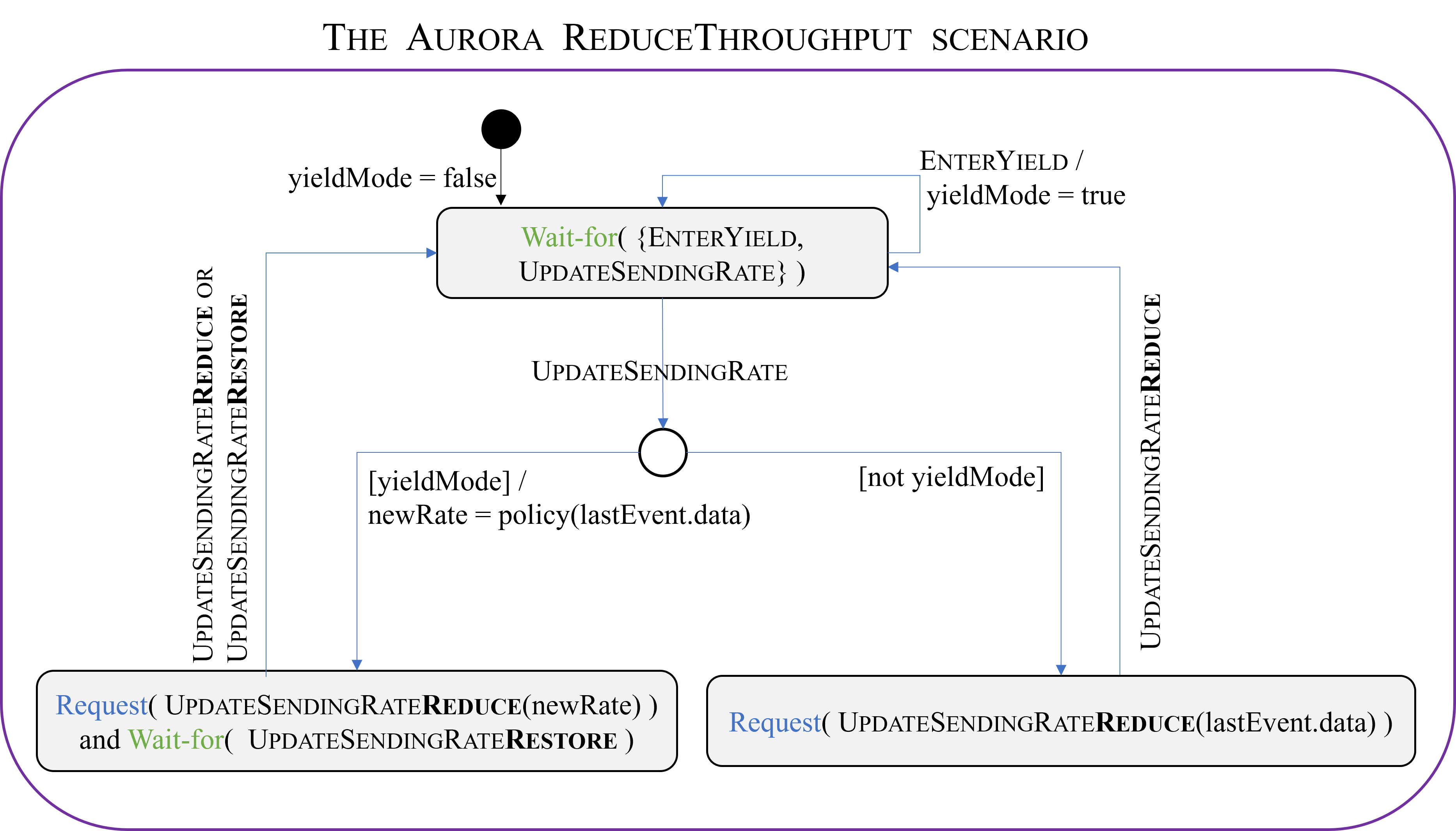
Figure 7: The Aurora ReduceThroughput scenario, described using Statecharts enhanced with SBM. The black circle specifies the initial state. The scenario waits-for EnterYield event to enter yield mode. If yield mode is enabled, the UpdateSendingRate event payload will be modified, and the UpdateSendingRateReduce will be requested. Otherwise, the payload is propagated as-is in the “proxy” UpdateSendingRateReduce event. The scenario waits for UpdateSendingRateRestore to return to its initial state, in case UpdateSendingRateReduce is blocked.

After entering scavenger mode and lowering the sending rate, a natural requirement is that the system eventually reverts to a higher sending rate, when scavenger mode is no longer required. To achieve this, we adjust the MonitorNetworkState scenario to dynamically identify this situation, and signal to the other scenarios that the system has entered restore mode, by requesting the event EnterRestore. We then introduce a second override scenario, RestoreThroughput, that can increase the protocol’s throughput according to one of two predefined policies: (i) an immediate return to the model’s original output; or (ii) a slow start policy [Contributors, 2022a].

The RestoreThroughput scenario waits-for the events EnterRestore, EnterYield and UpdateSendingRate. The first two events signal the scenario to enter/exit restore mode. When UpdateSendingRate is triggered and the scenario is in restore mode, it overrides the value according to the policy in use, and requests an output event with a modified value. Utilizing the UpdateSendingRateReduce event for this purpose would result in two, likely contradictory output events being requested at a single synchronization point. To avoid this, we introduce a new event, UpdateSendingRateRestore, to be requested by the RestoreThroughput scenario, while blocking the possible UpdateSendingRateReduce event at the synchronization point. This decision prioritizes ratio restoration over yielding (although any other prioritization rule could be used). Finally, in every scenario that requests/waits-for the UpdateSendingRateReduce event, we add a wait-for the UpdateSendingRateRestore event. In this manner, these scenarios can proceed with their execution despite being blocked.

3.3 Evaluation

For evaluation purposes, we implemented the scenario objects described in Sec. 3.2, and then used Aurora’s simulator to evaluate the enhanced model’s performance, compared to that of the original [Ashrov and Katz, 2023]. Our results, described below, indicate that the modified system successfully supports scavenger mode, although its internal DNN remained unchanged.

Fig. 8 depicts the sending rate requested by the Aurora $O_{DNN}$ scenario, following an input event QueryNextSendingRate, and the actual sending rate that was eventually returned to the simulator by the PCC-SBM protocol. We notice that initially, the two values coincide, indicating that no overriding is triggered — because the MonitorNetworkState scenario did not yet signal that the system should enter yield mode. However, once this signal occurs, the ReduceThroughput scenario overrides the sending rate, according to the fixed rate policy. After a while, the MonitorNetworkState detects that it is time to once again increase the sending rate, and signals that the system should enter restore mode. As a result, we see an increase, per the “slow start” restoration policy of RestoreThroughput. The ensuing back-and-forth switching between yield and restore modes demonstrates that the MonitorNetworkState scenario dynamically responds to changes in environmental conditions.

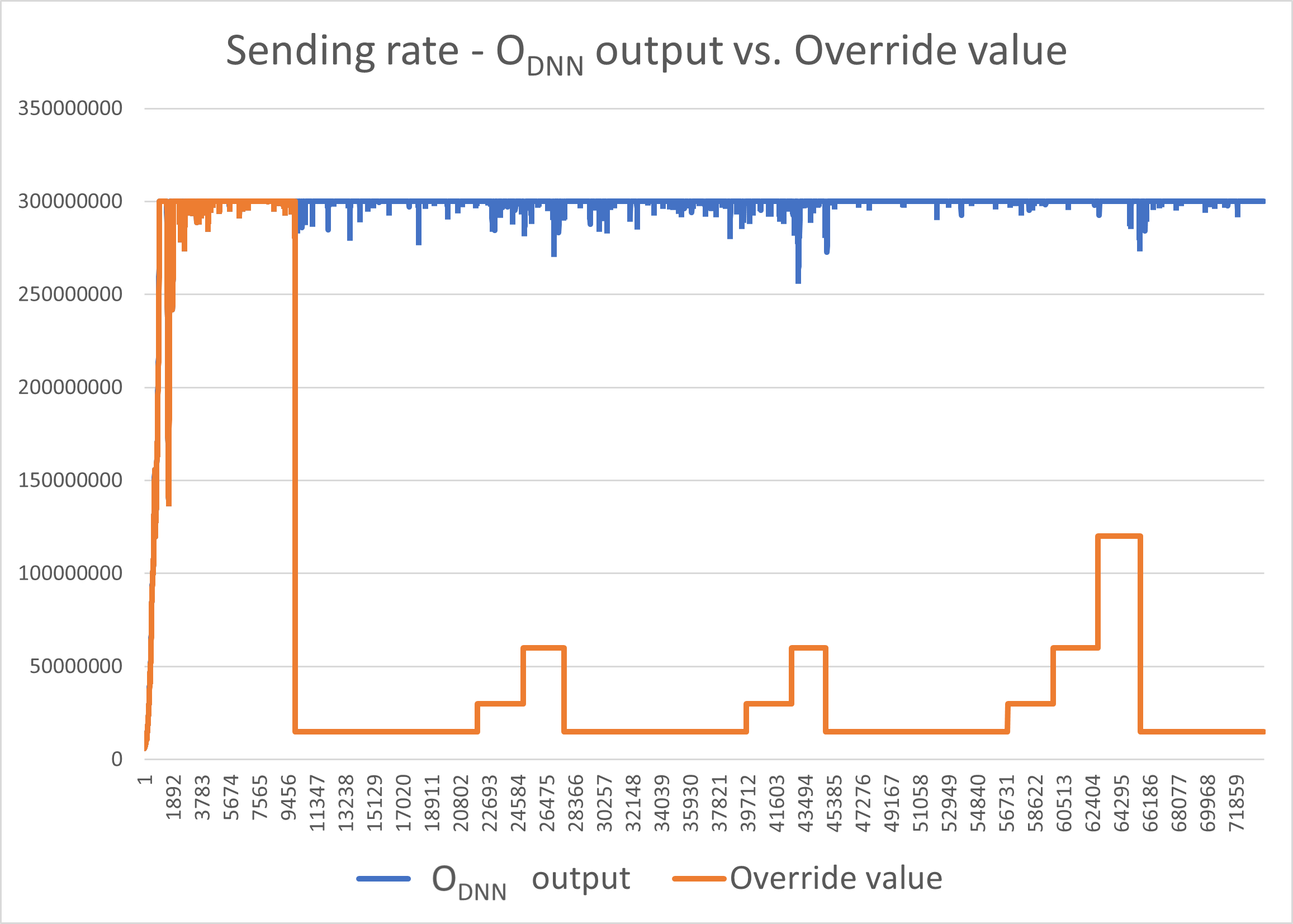
Figure 8: The Aurora $O_{DNN}$ original model output, vs. the values produced by the override scenarios. The policy used for reduction is an immediate decline to a fixed rate. The policy used for restoration is “slow start”.

In another experiment, we compared the throughput (MB/s) of the primary PCC-IXP protocol with that of the PCC-SBM protocol, when the two are executed in parallel. The results appear in Fig. 9. We observe that there is a resemblance between the overridden sending rate value seen in Fig. 8 and the actual throughput. When the MonitorNetworkState scenario signals to yield, the sending rate declines to a fixed value, which in turn leads to a fixed throughput. Additionally, when the sending rate increases after a signal to restore, the throughput of the protocol increases as well. Another interesting phenomenon is that when the PCC-SBM relinquishes bandwidth, the PCC-IXP increases its own throughput, which is the behavior we expect to see. We speculate that the yield of the PCC-SBM enabled this increase.

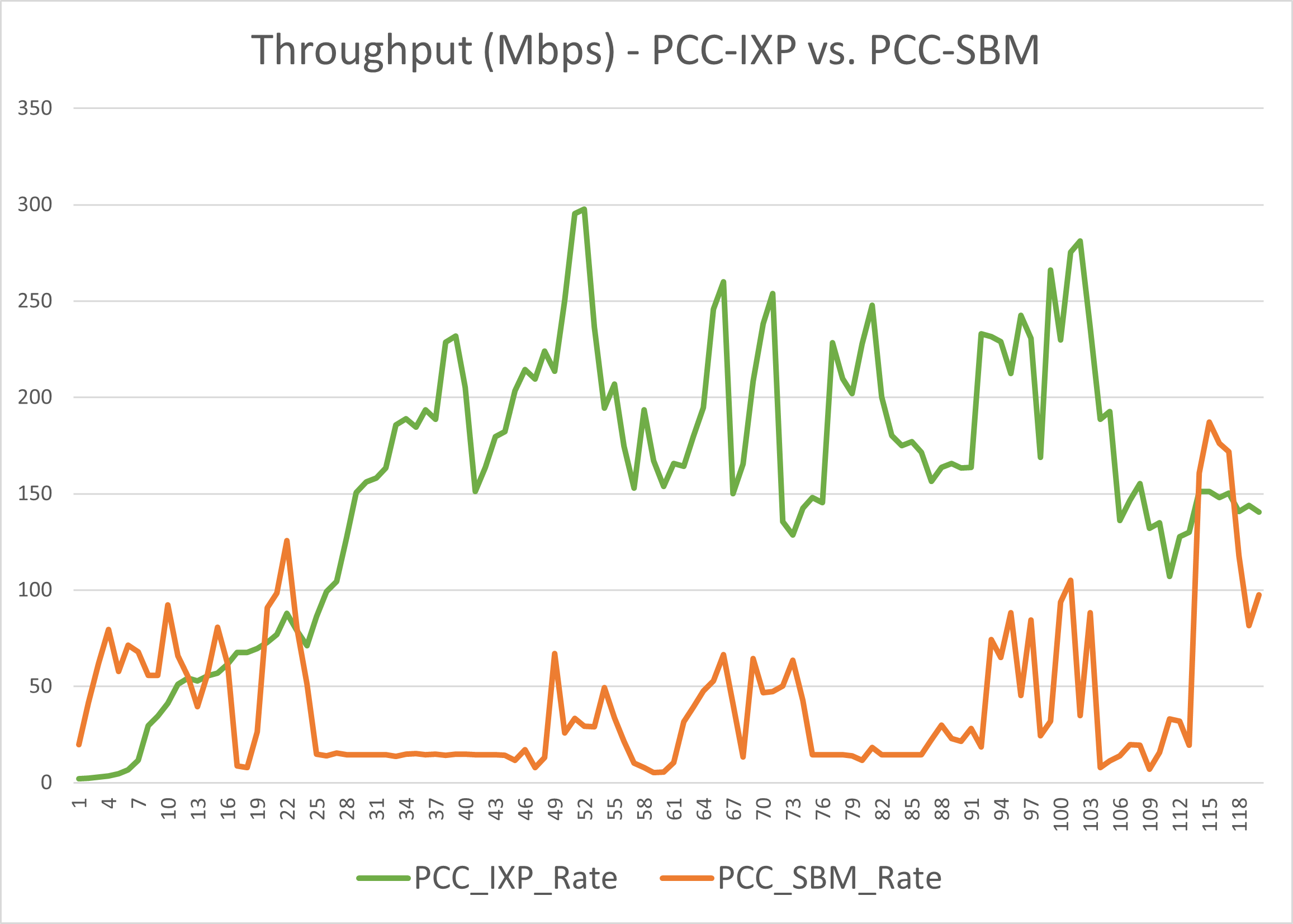
Figure 9: The recorded throughput (MB/s) of the PCC-IXP and PCC-SBM protocols, when executed in parallel using the PCC simulator.

4 CASE STUDY: THE ROBOTIS TURTLEBOT3 PLATFORM

For our second case study, we chose to enhance a DL system trained by Corsi et al. [Corsi et al., 2022a, Corsi et al., 2022b], which aims to solve a setup of the mapless navigation problem. The system contains a DNN agent whose goal is to navigate a Turtlebot 3 (Turtlebot) robot [Robotis, 2023, Amsters and Slaets, 2019] to a target destination, without colliding with obstacles. Contrary to classical planning, the robot does not hold a global map, but instead attempts to navigate using readings from its environment. A successful navigation policy must thus be dynamic, adapting to changes in local observations as the robot moves closer to its destination. DRL algorithms have proven successful in learning such a policy [Marchesini and Farinelli, 2020].

We refer to the DNN agent that controls the Turtlebot as TRL (for Turtlebot using RL). The agent learns a navigation policy iteratively: in each iteration, it is provided with a vector $v_{t}$ that comprises (i) normalized lidar scans of the robot’s distance from any nearby obstacles; and (ii) the angle and the distance of the robot from the target. The agent then evaluates its internal DNN on $v_{t}$, obtaining a vector $v_{a_{t}}$ that contains a probability distribution over the set of possible actions the Turtlebot can perform: moving forward, or turning left or right. For example, one possible vector is $v_{a_{t}}=[(\text{Forward}{},0.2),(\text{Left}{},0.5),(\text{Right}{},0.3)]$. Using this vector, the agent then randomly selects an action according to the distribution, navigates the Turtlebot, and receives a reward.

The DNN at the core of the TRL controller is trained and tested in a simulation environment that contains a sim-robot Turtlebot 3 burger [Robotis, 2023], and a single, fixed maze, created using the ROS2 framework [ROS, 2023] and the Unity3D engine [Unity, 2023]. In each session, the robot’s starting location is drawn randomly, which enables a diverse scan of the input space. The navigation session has four possible outcomes: (i) success; (ii) collision; (iii) timeout; or (iv) an unknown failure.

We selected the Turtlebot project as our second case study due to its reactive characteristics: it reads external information using its sensors, applies an internal logic to select the next action, and then acts by moving towards the target. SBM has previously been applied to model robot navigation and maze solving [Elyasaf, 2021, Ashrov et al., 2017], which strengthened our intuition that an enhancement of the Turtlebot with SBM is feasible. Next, we outline the objectives we aimed to achieve in this case study.

4.1 Integrating Turtlebot and SBM

Similarly to the Aurora case, our first goal was to instrument the Turtlebot DNN with the $O_{DNN}$ infrastructure, so that it could be composed with an SB model. This was achieved by using the Python implementation of SBM [Yaacov, 2020], and integrating it with the TRL code. We created a Sensor scenario that waits for the current state vector $v_{t}$, and injects an InputEvent containing $v_{t}$ into the SB model; and also an Actuator scenario that waits for an internal OutputEvent, and transmits its action as the one to be carried out by the Turtlebot.

Next, we proceeded to create the Turtlebot $O_{DNN}$ scenario for TRL. Unlike in the Aurora case, where the DNN would output a single chosen event, here the DNN outputs a probability distribution over the possible actions (a common theme in DRL-based systems [Sutton and Barto, 2018]). To accommodate this, we adjusted our $O_{DNN}$ scenario to request all the possible output events in the form of a vector $P_{at}$, which contains each possible action and its probability. We then modified SBM’s event selection mechanism to randomly select a requested output event from $P_{at}$, with respect to the induced probability distribution. The mechanism then triggers the OutputEvent, which contains in its payload the selected action and its probability. During modeling and experimentation, the scenario can assign any probability distribution (e.g., uniform) to the DNN’s output events; and during deployment, these values are computed using the actual DNN (see Fig. 10). If the event selection mechanism selects an event that is blocked, the selection is repeated, until a non-blocked event is selected. If there are no enabled events, then the system is deadlocked and the program ends. Using this approach, our Turtlebot controller could successfully navigate in various mazes.

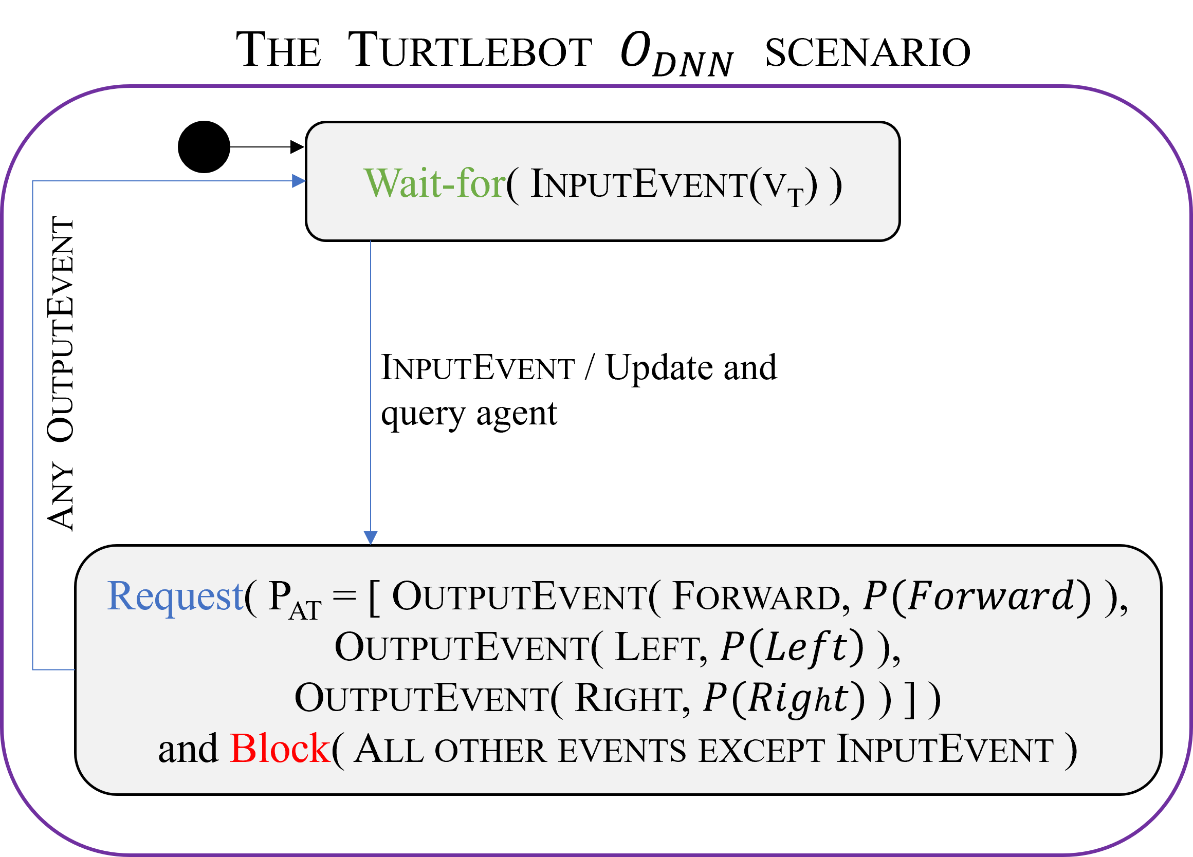
Figure 10: The Turtlebot $O_{DNN}$ scenario. The scenario waits for an InputEvent containing $v_{t}$, provides it to the agent, and receives a vector $P_{at}$ of possible actions and probabilities. It then proceeds to request all the output events from the ESM using $P_{at}$. At the synchronization point, the ESM executes the Turtlebot $O_{DNN}$ event selection strategy, and one possible OutputEvent is triggered.

Once the $O_{DNN}$ infrastructure was in place, we verified that the augmented program’s performance was similar to that of the original agent. This was achieved by comparing the models pre-trained by [Corsi et al., 2022a] to our SBM-enhanced version, and checking that both agents obtained similar success rates on various mazes.

4.2 A Conservative Controller

For our second goal, we sought to increase the model’s safety, by implementing a basic override rule, OverrideObstacleAhead, which would prevent the Turtlebot from colliding with an obstacle that is directly ahead. This can be achieved by analyzing the DNN’s inputs, which include the lidar readings, and identifying cases where a move forward would guarantee a collision; and then blocking this move, forcing the system to select a different action. An illustration of this simple override rule appears in Fig. 11.

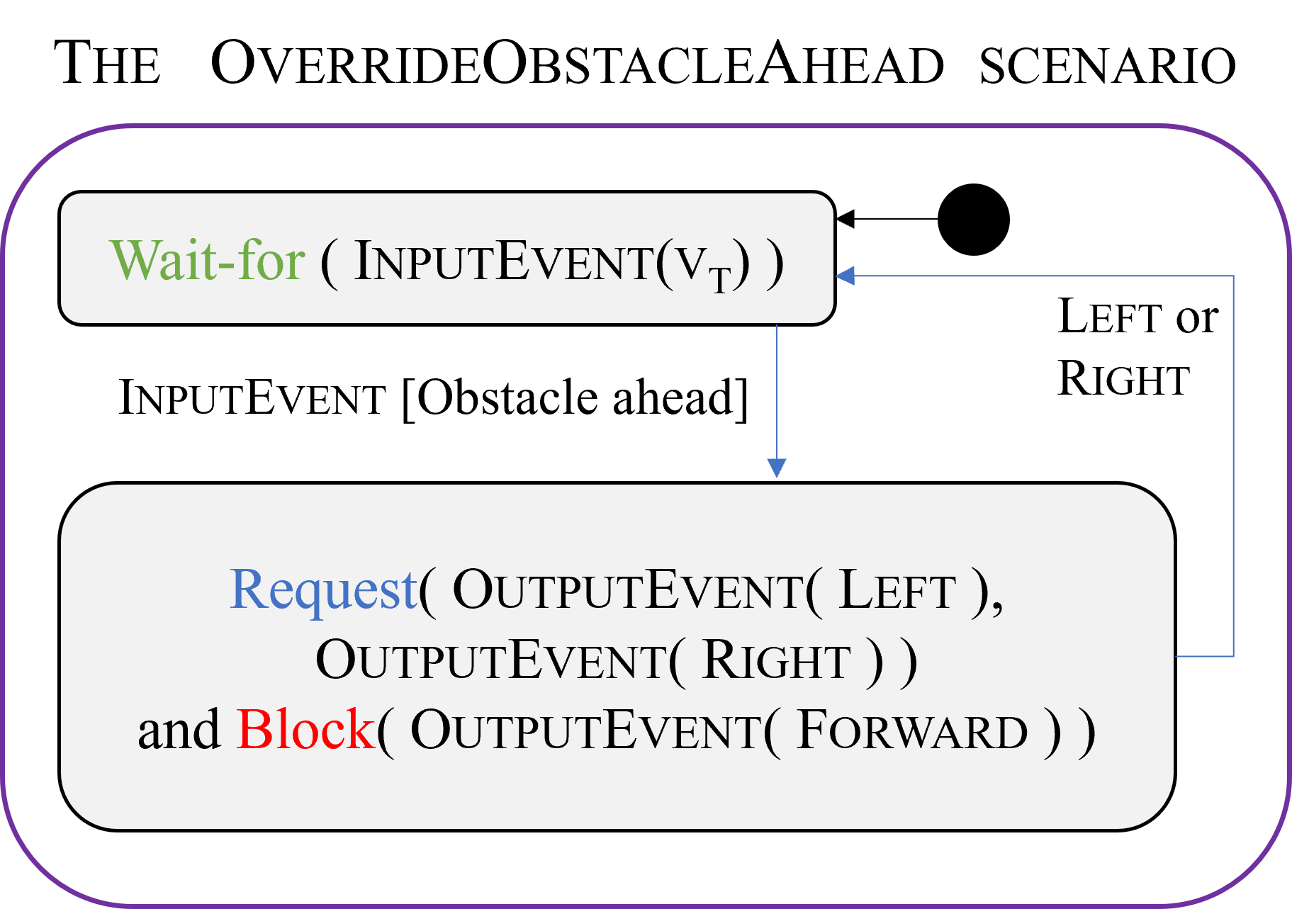
Figure 11: The OverrideObstacleAhead scenario waits for an InputEvent containing $v_{t}$, and inspects the lidar sensors facing forward readings. If $distance<0.22$, moving forward will cause a collision. Therefore the scenario blocks the OutputEvent(Forward) event.

As we were experimenting with the Turtlebot and various override rules, we noticed the following, interesting pattern. Recall that a Turtlebot agent learns a policy, which, for a given state $s_{t}$, produces a probability distribution over the actions, $a_{t}=[P(\text{Forward}{}),P(\text{Left}{}),P(\text{Right}{})]$. We can regard this vector as the agent’s confidence levels that each of the possible actions will bring the Turtlebot closer to its goal. The random selection that follows takes these confidence levels into account, and is more likely to select an action that the agent is confident about; but this is not always the case. Specifically, we observed that for “weaker” models, e.g. models with about a 50% success rate, the agent would repeatedly select actions with a low confidence score, which would often lead to a collision. This observation led us to design our next override scenario, ConservativeAction, which is intended to force the agent to select actions only when their confidence score meets a certain threshold.

Ideally, we wish for ConservativeAction to implement the following behavior: (i) wait-for the OutputEvent being selected (ii) examine whether the confidence score in its payload is below a certain threshold, and if so, (iii) apply blocking to ensure that a different OutputEvent, with a higher score, is selected for triggering. This method again requires that the override scenario be able to inspect the content of the OutputEvent being triggered in the current time step.

To overcome this issue, we add a new, proxy event called OutputEventProxy, and adjust all existing scenarios that would previously wait for OutputEvent to wait for this new event, instead. Then, we have the ConservativeAction scenario wait-for the input event to $O_{DNN}$, and have it replay that event to initiate additional evaluations of the DNN, and the ensuing random picking of the OutputEvent, until an acceptable output action is selected. When this occurs, the ConservativeAction scenario propagates the selected action as an OutputEventProxy event.

4.3 Evaluation

For evaluation purposes, we trained a collection of agents, $C_{agents}$, using the technique of Corsi et al. [Corsi et al., 2022b]. These agents had varying success rates, ranging from $4\%$ to $96\%$. Next, we compared the performance of these agents to their performance when enhanced by our SB model.

In the first experiment, we disabled our override rule, and had every agent in $C_{agents}$ solve a maze from 100 different random starting points. The statistics we measured were:

• num_of_solved: the number of times the agent reached the target.

• num_of_collision: the number of times the agent collided with an obstacle.

• avg_num_of_steps: the average number of steps the agent performed in a successful navigation.

We then repeated this setting with the ConservativeAction scenario enabled.

The experiment’s results are summarized in Fig. 12, and show that enabling the override rule leads to a significant reduction in the number of collisions. We notice that, as the agent’s success rate increases, the improvement rate decreases. One hypothesis for this behavior could be that “stronger” models are more confident in their recommended actions, thus requiring fewer activations of the override rule.

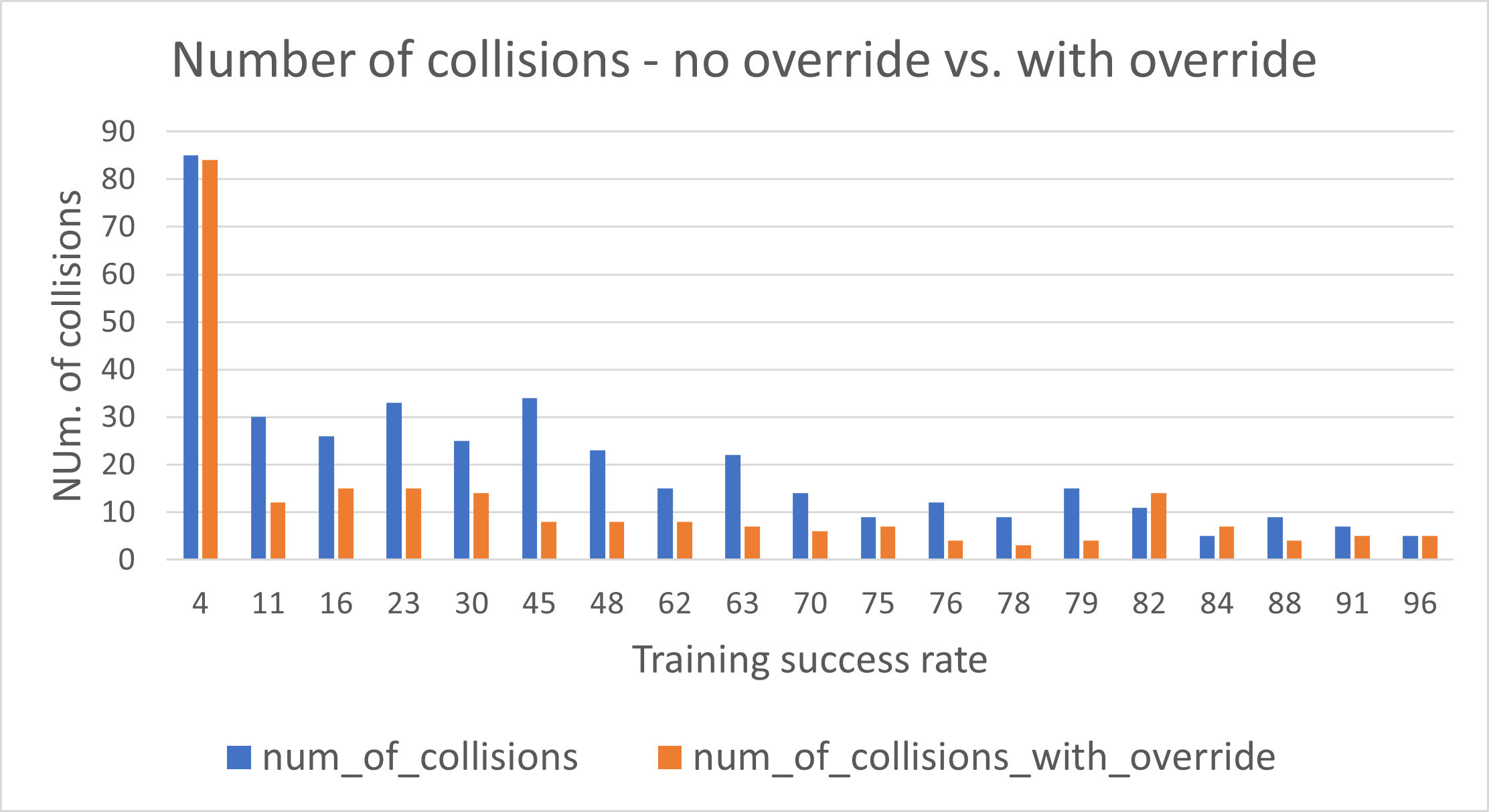
Figure 12: Comparing the number of collisions when the ConservativeAction override is disabled and then enabled.

Fig. 13 portrays a general improvement in the agent’s success rate when the override rule is enabled, which is (unsurprisingly) correlated with the reduction in the number of collisions. A possible explanation is that “mediocre” agents, i.e. those with success rates in the range between $16\%$ and $70\%$, learned policies that are good enough to navigate towards the target, but which require some assistance in order to avoid obstacles along the way.

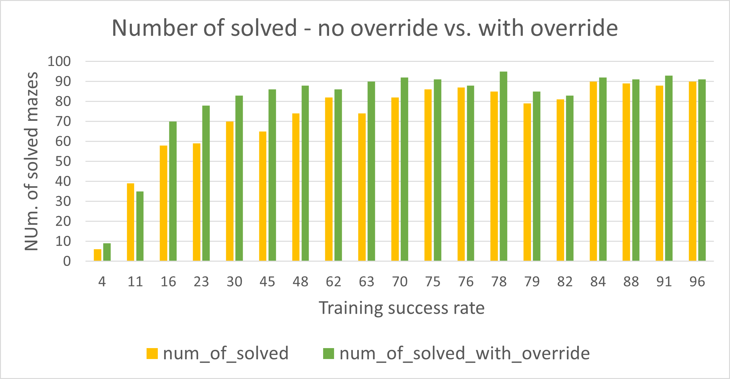
Figure 13: Comparing the num. of solved mazes when the ConservativeAction override is disabled and then enabled.

Fig. 14 depicts a reduction in the average number of steps required for an agent to solve the maze, when the override scenario is enabled. This somewhat surprising result indicates that although our agents can successfully solve mazes, the ConservativeAction scenario renders their navigation more efficient. We speculate that for these agents, selecting actions with low confidence scores leads to redundant steps.

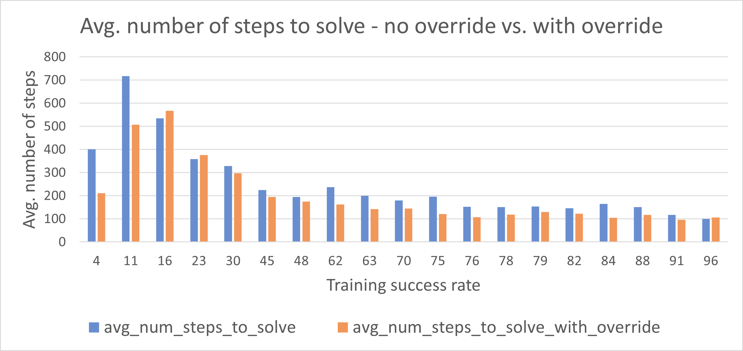
Figure 14: Comparing the average number of steps to solve when the ConservativeAction override is disabled and then enabled.

5 INTRODUCING MODIFIER SCENARIOS

5.1 Motivation

In both of our case studies, we needed to create scenarios capable of reasoning about the events being requested in the current time step — which we resolved by introducing new, “proxy” events. However, such a solution has several drawbacks. First, it entails extensive renaming of existing events, and the modification of existing scenarios, which goes against the incremental nature of SBM [Harel et al., 2012]. Second, once added, the override scenario becomes a crucial component in the $O_{DNN}$ infrastructure, without which the system cannot operate; and in the common case where the override rule is not triggered, this incurs unnecessary overhead. Third, it is unclear how to support the case where several scenarios are required. These drawbacks indicate that the “proxy” solution is complex, costly, and leaves much to be desired.

In order to address this need and allow users to design override rules in a more convenient manner, we propose here to extend the idioms of SBM in a way that will support modifier scenarios: scenarios that are capable of observing and modifying the current event, as it is being selected for triggering. A formal definition appears below.

5.2 Defining Modifier Scenarios

We extend the definitions of SBM from Sec. 2 with a new type of scenario, named a modifier scenario. A modifier scenario is formally defined as a tuple $O_{\text{modifier}}{}=\langle Q^{M},q_{0}^{M},\delta^{M},f^{M}\rangle$, where:

• $Q^{M}$ is a set of states representing synchronization points.

• $q_{0}^{M}$ is the initial state.

• $\delta^{M}:Q^{M}\times E\to Q^{M}$ is a deterministic transition function, indicating how the scenario reacts when an event is triggered.

• $f^{M}:Q^{M}\times 2^{E}\times 2^{E}\to E$ is a function that maps a state, a set of observed requested events, and a set of observed blocked events into an event from the set $E$. $f^{M}$ can operate in a deterministic, well-defined manner, or in a randomized manner to select a suitable event from $E$.

Intuitively, the modifier thread can use its function $f^{M}$ at a synchronization point to affect the selection of the current event.

Let $M=\{O^{1},...,O^{n},O_{\text{modifier}}{}\}$ be a behavioral model, where $n\in N$, each $O^{i}=\langle Q^{i},q_{0}^{i},\delta^{i},R^{i},B^{i}\rangle$ is an ordinary scenario object, and $O_{\text{modifier}}{}$ is a modifier scenario object. In order to define the semantics of $M$, we construct the labeled transition system $LTS(M)=\langle Q,q_{0},\delta,f^{M}\rangle$, where:

• $Q:=Q^{1}\times...\times Q^{n}\times Q^{M}$ is the set of states.

• $q_{0}:=\langle q_{0}^{1},...,q_{0}^{n},q_{0}^{M}\rangle\in Q$ is the initial state.

• $f^{M}:=f^{M}$ is the modification function of $O_{\text{modifier}}{}$.

• $\delta:Q\times E\to Q$ is a deterministic transition function, defined for all $q=\langle q^{1},...,q^{n},q^{M}\rangle\in Q$ and $e\in E$ by

  $$\delta(q,e):=\langle\delta^{1}(q^{1},e),...,\delta^{n}(q^{n},e),\delta^{M}(q^{M},e)\rangle$$

An execution of $P$ is an execution of $LTS(M)$. The execution starts from the initial state $q_{0}$, and in each state $q\in Q$, the event selection mechanism collects the sets of requested and blocked events, namely $R(q):=\bigcup\limits_{i=1}^{n}R^{i}(q^{i})$ and $B(q):=\bigcup\limits_{i=1}^{n}B^{i}(q^{i})$.

The set of enabled events at synchronization point $q$ is $E(q)=R(q)\setminus B(q)$. If $E(q)=\emptyset$ then the system is deadlocked. Otherwise, the ESM allows the modifier scenario to affect event selection, by applying $f^{M}$ and selecting the event:

$$e=f^{M}(q,R(q),B(q)).$$

The ESM then triggers $e$, and notifies the relevant scenarios. By convention, we require that $f^{M}$ does not select an event that is currently blocked; although it can select events that are not currently requested. The state of $LTS(M)$ is then updated according to $e$. The execution of $LTS(M)$ is formally recorded as a sequence of triggered events (a run). For simplicity, we assume that there is a single $O_{\text{modifier}}{}$ object in the model, although in practice it can be implemented using a collection of scenarios.

5.3 Revised Override Scenarios

We extend the definition of an override rule over a network $N$, into a tuple $\langle P,Q,f\rangle$, where: (i) $P(x)$is a predicate over the network’s input vector $x$; (ii) $Q(N(x))$is a predicate over the network’s output vector $N(x)$; and (iii) $f:\mathbb{O}\to\mathbb{O}$is a function that replaces the proposed network output event with a new output event. Using a modifier scenario $O_{\text{modifier}}{}$, we can now implement this more general form of an override rule within an SB model. As an illustrative example, we change the override rule from Sec. 2.2, to consider the network’s output as well:

$$\langle x_{1}>x_{2},y_{2}>1,f(y_{i})\to y_{1}\rangle$$

Note that this definition differs from the original: it takes into account the currently selected output event and its value. Also, it contains a function $f$ that, whenever the predicates hold, maps a network-selected output into action $y_{1}$. An updated version of the override rule, implemented as a modifier scenario, appears in Fig. 15. To support the ability to observe output event $e_{o}$’s internal value, the event contains a payload of the calculated output neurons’ values.

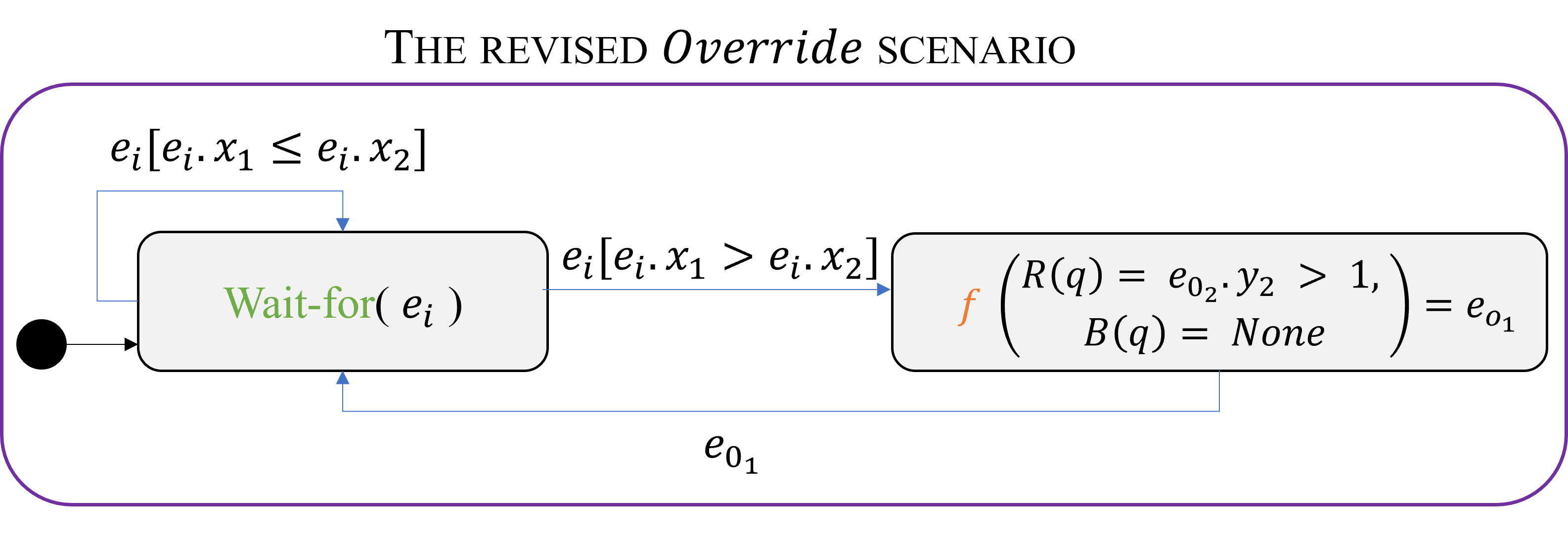
Figure 15: An $O_{\text{modifier}}{}$ scenario object for enforcing the override rule that whenever $x_{1}>x_{2}$ and $y_{2}>1$, output event $e_{o_{1}}$ should be triggered. The scenario waits for the input event to satisfy the predicate, and then proceeds to the state where it declares a modification. The first argument to the modification function $f$ is the output event and assignment that the scenario would like to modify. The second argument to the function is the set of blocked events: None, in our case. The return value from the function is the output event, $e_{o_{1}}$. At the synchronization point, the ESM collects the requested and blocked events, applies the $f$ function of the modifier scenario, and then notifies the relevant scenarios that $e_{o_{1}}$ output event has been selected for triggering.

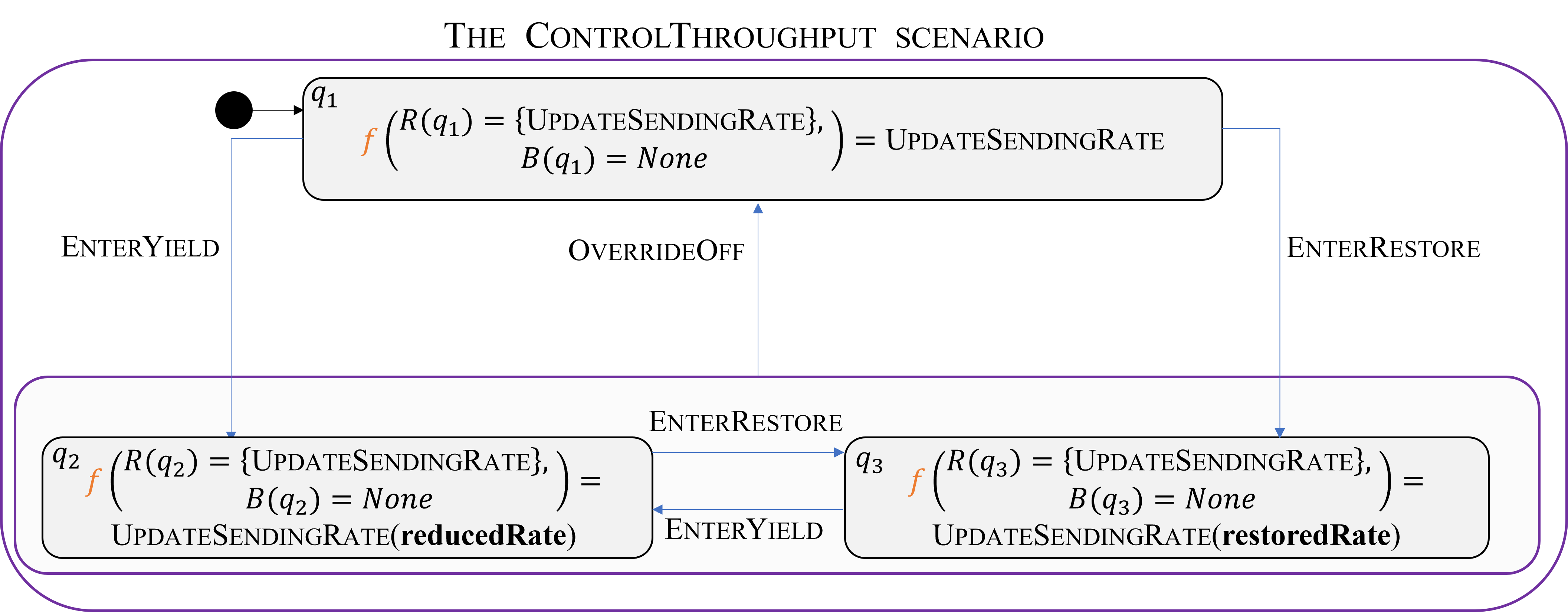
Figure 16: The ControlThroughput override scenario. The scenario waits-for events {OverrideOff,EnterYield,EnterRestore} in each state, and transitions subsequently. It also observes and possibly modifies the UpdateSendingRate event using its $f$ function depending on the current state $q_{i}$, $R(q_{i})$ and $B(q_{i})$. E.g., if we are in $q_{2}$, and UpdateSendingRate is requested but not blocked, its value will be modified according to the reduce policy. Note that the modification of the UpdateSendingRate does not result in a transition to a different state.

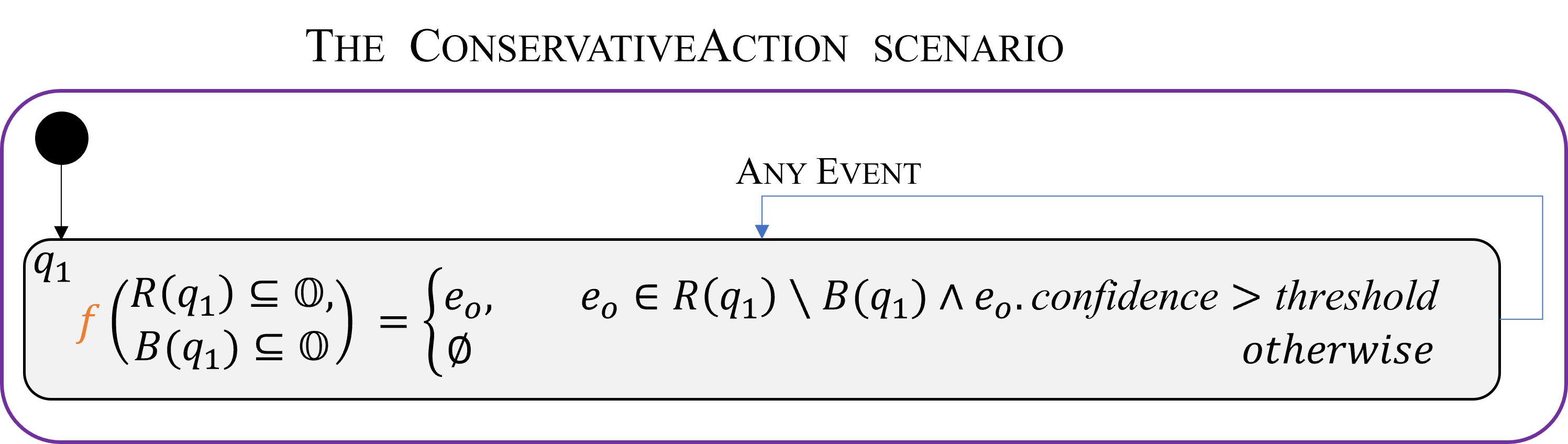
Figure 17: The revised ConservativeAction scenario. The scenario observes all possible subsets of the output events $\mathbb{O}$ that are requested or blocked at state $q_{1}$. Concretely, at each synchronization point, the ESM launches $f$ with a specific set of the requested and blocked output events. The function $f$ is only concerned with the set of enabled (requested and not blocked) output events. From these possible output events, $f$ randomly selects an event $e_{o}$ according to this policy: (i) if the selected event is above the threshold, $f$ passes the event as-is; and (ii) if the selected event is below the threshold, $f$ randomly selects a different possible output event which is above the threshold. The ESM then notifies the relevant scenarios of the selected output event. If no such event exists, the program is in a deadlock, in which case the scenario can reduce the threshold to find a possible event. The scenario remains in its state $q_{1}$ whenever any event is triggered.

With the updated override rule definition, we now refactor the scenarios from Sec. 3.2. First, we restore UpdateSendingRate to its original role as an output event (as opposed to a proxy event). Second, we modify the MonitorNetworkState scenario to request three events that signal the current throughput state: (i) OverrideOff, which signals that the sending rate should be forwarded as-is; and (ii) EnterYieldand (iii) EnterRestore, which signal that the sending rate should be overridden by the yield/restore policy. Third, we introduce the ControlThroughput override scenario, replacing ReduceThroughput and RestoreThroughput. This scenario waits-for a signal on the current throughput state, and transitions between the internal states that represent it. The scenario uses function $f$ to observe the requested event UpdateSendingRate in each state. When the output event UpdateSendingRate is requested, $f$ is executed and receives the requested and blocked events as parameters. If the event is blocked, we are in a deadlock. If the scenario is in the OverrideOff state, the function returns the event as-is. If the scenario is in the EnterYield/ EnterRestore states, the scenario returns an UpdateSendingRate event with a sending rate that is modified according to the matching policy. The revised UpdateSendingRate event is then triggered, and all relevant scenarios proceed with their execution. Fig. 16 depicts the new ControlThroughput scenario.

We now revise the set of scenarios we implemented to support the TRL project 4 and the conservative override rule 4.2. The first modification is to restore the OutputEvent event to its original role as an output, instead of a proxy event. We then use the $f$ function to simplify the ConservativeAction scenario. Recall that originally, the scenario waited for the InputEvent, for the purpose of re-playing the $O_{DNN}$ evaluation if the selected OutputEvent was below the threshold. The revised scenario can define an $f$ that will observe the set of requested output events, and then randomly select an output event that exceeds the threshold, and which is not blocked. If there are no possible output events, the system is deadlocked. From a practical point of view, the scenario can reduce the threshold to avoid this situation (assuming that $R(q)\setminus B(q)$ is not empty). Fig. 17 displays the revised ConservativeAction scenario.

In summary, we have successfully revised the override rules from our two case studies utilizing the $O_{\text{modifier}}{}$ extension. First, this new and more powerful definition has enabled us to implement the rules without “proxy” events. This change reduces the high coupling between the scenarios of the original implementation. Second, the redesigned models offer a more compact and direct approach: (i) the two override rules from the Aurora case study were reduced to a single scenario; and (ii) the TRL override rule contains a single synchronization point. These characteristics are more in line with the SBM spirit that views scenarios as simple and self-contained components. Moving forward, we plan to enhance the existing SBM packages with the $O_{\text{modifier}}{}$ extension.

6 RELATED WORK

Override rules are becoming an integral part of many DRL-based systems [Katz, 2020]. The concept is closely related to that of shields and runtime monitors, which have been extensively used in the field of robotics [Phan et al., 2017], drones [Desai et al., 2018], and many others [Hamlen et al., 2006, Falcone et al., 2011, Schierman et al., 2015, Ji and Lafortune, 2017, Wu et al., 2018]. We regard our work as another step towards the goal of effectively creating, and maintaining, override rules for complex systems.

Although our focus here has been on designing override rules using SBM, other modeling formalisms could be used just as well. Notable examples include the publish-subscribe framework [Eugster et al., 2003], aspect oriented programming [Kiczales et al., 1997], and the BIP formalism [Bliudze and Sifakis, 2008]. A key property of SBM, which seems to render it a good fit for override rules, is the native idiom support for blocking events [Katz, 2020]; although similar support could be obtained, using various constructs, in other formalisms.

7 CONCLUSION

As DNNs are increasingly being integrated into complex systems, there is a need to maintain, extend and adjust them — which has given rise to the creation of override rules. In this work, we sought to contribute to the ongoing effort of facilitating the creation of such rules, through two extensive case studies. Our efforts exposed a difficulty in an existing, SBM-based method for designing guard rules, which we were then able to mitigate by extending the SBM framework itself. We hope that this effort, and others, will give rise to formalisms that are highly equipped for supporting engineers in designing override rules for DNN-based systems.

REFERENCES

- Amsters and Slaets, 2019 Amsters, R. and Slaets, P. (2019). Turtlebot 3 as a Robotics Education Platform. In Proc. 10th Int. Conf. on Robotics in Education (RiE), pages 170–181.
- Ashrov et al., 2017 Ashrov, A., Gordon, M., Marron, A., Sturm, A., and Weiss, G. (2017). Structured Behavioral Programming Idioms. In Proc. 18th Int. Conf. on Enterprise, Business-Process and Information Systems Modeling (BPMDS), pages 319–333.
- Ashrov and Katz, 2023 Ashrov, A. and Katz, G. (2023). Enhancing Deep Learning with Scenario-Based Override Rules — Code Base. https://github.com/adielashrov/Enhance-DL-with-SBM-Modelsward2023.
- Ashrov et al., 2015 Ashrov, A., Marron, A., Weiss, G., and Wiener, G. (2015). A Use-Case for Behavioral Programming: an Architecture in JavaScript and Blockly for Interactive Applications with Cross-Cutting Scenarios. Science of Computer Programming, 98:268–292.
- Avni et al., 2019 Avni, G., Bloem, R., Chatterjee, K., Henzinger, T., Konighofer, B., and Pranger, S. (2019). Run-Time Optimization for Learned Controllers through Quantitative Games. In Proc. 31st Int. Conf. on Computer Aided Verification (CAV), pages 630–649.
- Bar-Sinai et al., 2018a Bar-Sinai, M., Weiss, G., and Shmuel, R. (2018a). BPjs—a Framework for Modeling Reactive Systems using a Scripting Language and BP. Technical Report. http://arxiv.org/abs/1806.00842.
- Bar-Sinai et al., 2018b Bar-Sinai, M., Weiss, G., and Shmuel, R. (2018b). BPjs: an Extensible, Open Infrastructure for Behavioral Programming Research. In Proc. 21st ACM/IEEE Int. Conf. on Model Driven Engineering Languages and Systems (MODELS), pages 59–60.
- Bliudze and Sifakis, 2008 Bliudze, S. and Sifakis, J. (2008). A Notion of Glue Expressiveness for Component-Based Systems. In Proc. 19th Int. Conf. on Concurrency Theory (CONCUR), pages 508–522.
- Bojarski et al., 2016 Bojarski, M., Del Testa, D., Dworakowski, D., Firner, B., Flepp, B., Goyal, P., Jackel, L., Monfort, M., Muller, U., Zhang, J., Zhang, X., Zhao, J., and Zieba, K. (2016). End to End Learning for Self-Driving Cars. Technical Report. http://arxiv.org/abs/1604.07316.
- Collobert et al., 2011 Collobert, R., Weston, J., Bottou, L., Karlen, M., Kavukcuoglu, K., and Kuksa, P. (2011). Natural Language Processing (almost) from Scratch. Journal of Machine Learning Research, 12:2493–2537.
- Contributors, 2022a Contributors, W. (2022a). TCP Slow start — Wikipedia, The Free Encyclopedia. https://en.wikipedia.org/wiki/TCP˙congestion˙control#Slow˙start.
- Contributors, 2022b Contributors, W. (2022b). Wall follower — Maze-solving algorithm — Wikipedia, The Free Encyclopedia. https://en.wikipedia.org/wiki/Maze-solving˙algorithm#Wall˙follower.
- Corsi et al., 2022a Corsi, D., Yerushalmi, R., Amir, G., Farinelli, A., Harel, D., and Katz, G. (2022a). Constrained Reinforcement Learning for Robotics via Scenario-Based Programming. Technical Report. https://arxiv.org/abs/2206.09603.
- Corsi et al., 2022b Corsi, D., Yerushalmi, R., Amir, G., Farinelli, A., Harel, D., and Katz, G. (2022b). Constrained Reinforcement Learning for Robotics via Scenario-Based Programming — Code Base. https://github.com/d-corsi/ScenarioBasedRL.
- Desai et al., 2018 Desai, A., Ghosh, S., Seshia, S. A., Shankar, N., and Tiwari, A. (2018). Soter: Programming Safe Robotics System using Runtime Assurance. Technical Report. http://arxiv.org/abs/1808.07921.
- Dong et al., 2015 Dong, M., Li, Q., Zarchy, D., Godfrey, P. B., and Schapira, M. (2015). PCC: Re-Architecting Congestion Control for Consistent High Performance. In Proc. 12th USENIX Symposium on Networked Systems Design and Implementation (NSDI), pages 395–408.
- Dong et al., 2018 Dong, M., Meng, T., Zarchy, D., Arslan, E., Gilad, Y., Godfrey, B., and Schapira, M. (2018). PCC Vivace: Online-Learning Congestion Control. In Proc. 15th USENIX Symposium on Networked Systems Design and Implementation (NSDI), pages 343–356.
- Elyasaf, 2021 Elyasaf, A. (2021). Context-Oriented Behavioral Programming. Information and Software Technology, 133:106504.
- Eugster et al., 2003 Eugster, P., Felber, P., Guerraoui, R., and Kermarrec, A.-M. (2003). The Many Faces of Publish/Subscribe. ACM Computing Surveys (CSUR), 35(2):114–131.
- Falcone et al., 2011 Falcone, Y., Mounier, L., Fernandez, J., and Richier, J. (2011). Runtime Enforcement Monitors: Composition, Synthesis, and Enforcement Abilities. Journal on Formal Methods in System Design (FMSD), 38(3):223–262.
- Goodfellow et al., 2016 Goodfellow, I., Bengio, Y., and Courville, A. (2016). Deep learning. MIT press.
- Gordon et al., 2012 Gordon, M., Marron, A., and Meerbaum-Salant, O. (2012). Spaghetti for the Main Course? Observations on the Naturalness of Scenario-Based Programming. In Proc. 17th Conf. on Innovation and Technology in Computer Science Education (ITICSE), pages 198–203.
- Hamlen et al., 2006 Hamlen, K., Morrisett, G., and Schneider, F. (2006). Computability Classes for Enforcement Mechanisms. ACM Transactions on Programming Languages and Systems (TOPLAS), 28(1):175–205.
- Harel, 1986 Harel, D. (1986). A Visual Formalism for Complex Systems. Science of Computer Programming, 8(3).
- Harel et al., 2013 Harel, D., Kantor, A., and Katz, G. (2013). Relaxing Synchronization Constraints in Behavioral Programs. In Proc. 19th Int. Conf. on Logic for Programming, Artificial Intelligence and Reasoning (LPAR), pages 355–372.
- Harel and Katz, 2014 Harel, D. and Katz, G. (2014). Scaling-Up Behavioral Programming: Steps from Basic Principles to Application Architectures. In Proc. 4th SPLASH Workshop on Programming based on Actors, Agents and Decentralized Control (AGERE!), pages 95–108.
- Harel et al., 2015a Harel, D., Katz, G., Lampert, R., Marron, A., and Weiss, G. (2015a). On the Succinctness of Idioms for Concurrent Programming. In Proc. 26th Int. Conf. on Concurrency Theory (CONCUR), pages 85–99.
- Harel et al., 2016 Harel, D., Katz, G., Marelly, R., and Marron, A. (2016). An Initial Wise Development Environment for Behavioral Models. In Proc. 4th Int. Conf. on Model-Driven Engineering and Software Development (MODELSWARD), pages 600–612.
- Harel et al., 2018 Harel, D., Katz, G., Marelly, R., and Marron, A. (2018). Wise Computing: Toward Endowing System Development with Proactive Wisdom. IEEE Computer, 51(2):14–26.
- Harel et al., 2014 Harel, D., Katz, G., Marron, A., and Weiss, G. (2014). Non-Intrusive Repair of Safety and Liveness Violations in Reactive Programs. Transactions on Computational Collective Intelligence (TCCI), 16:1–33.
- Harel et al., 2015b Harel, D., Katz, G., Marron, A., and Weiss, G. (2015b). The Effect of Concurrent Programming Idioms on Verification. In Proc. 3rd Int. Conf. on Model-Driven Engineering and Software Development (MODELSWARD), pages 363–369.
- Harel et al., 2022 Harel, D., Marron, A., and Sifakis, J. (2022). Creating a Foundation for Next-Generation Autonomous Systems. IEEE Design & Test.
- Harel et al., 2010 Harel, D., Marron, A., and Weiss, G. (2010). Programming Coordinated Behavior in Java. In Proc. European Conf. on Object-Oriented Programming (ECOOP), pages 250–274.
- Harel et al., 2012 Harel, D., Marron, A., and Weiss, G. (2012). Behavioral programming. Communications of the ACM, 55(7):90–100.
- Jay et al., 2019 Jay, N., Rotman, N., Godfrey, B., Schapira, M., and Tamar, A. (2019). A Deep Reinforcement Learning Perspective on Internet Congestion Control. In Proc. Int. Conf. on Machine Learning (ICML), pages 3050–3059.
- Ji and Lafortune, 2017 Ji, Y. and Lafortune, S. (2017). Enforcing Opacity by Publicly Known Edit Functions. In Proc. 56th IEEE Annual Conf. on Decision and Control (CDC), pages 12–15.
- Julian et al., 2016 Julian, K., Lopez, J., Brush, J., Owen, M., and Kochenderfer, M. (2016). Policy Compression for Aircraft Collision Avoidance Systems. In Proc. IEEE/AIAA 35th Digital Avionics Systems Conference (DASC), pages 1–10.
- Jumper et al., 2021 Jumper, J., Evans, R., Pritzel, A., Green, T., Figurnov, M., Ronneberger, O., Tunyasuvunakool, K., Bates, R., Žídek, A., Potapenko, A., et al. (2021). Highly Accurate Protein Structure Prediction with Alphafold. Nature, 596(7873):583–589.
- Katz, 2013 Katz, G. (2013). On Module-Based Abstraction and Repair of Behavioral Programs. In Proc. 19th Int. Conf. on Logic for Programming, Artificial Intelligence and Reasoning (LPAR), pages 518–535.
- Katz, 2020 Katz, G. (2020). Guarded Deep Learning using Scenario-Based Modeling. In Proc. 8th Int. Conf. on Model-Driven Engineering and Software Development (MODELSWARD), pages 126–136.
- Katz, 2021a Katz, G. (2021a). Augmenting Deep Neural Networks with Scenario-Based Guard Rules. Communications in Computer and Information Science (CCIS), 1361:147–172.
- Katz, 2021b Katz, G. (2021b). Behavioral Programming in C++. https://github.com/adielashrov/bpc.
- Katz et al., 2019 Katz, G., Marron, A., Sadon, A., and Weiss, G. (2019). On-the-Fly Construction of Composite Events in Scenario-Based Modeling Using Constraint Solvers. In Proc. 7th Int. Conf. on Model-Driven Engineering and Software Development (MODELSWARD), pages 143–156.
- Kiczales et al., 1997 Kiczales, G., Lamping, J., Mendhekar, A., Maeda, C., Lopes, C., Loingtier, J.-M., and Irwin, J. (1997). Aspect-Oriented Programming. In Proc. European Conf. on Object-Oriented Programming (ECOOP), pages 220–242.
- Marchesini and Farinelli, 2020 Marchesini, E. and Farinelli, A. (2020). Discrete Deep Reinforcement Learning for Mapless Navigation. In Proc. IEEE Int. Conf. on Robotics and Automation (ICRA), pages 10688–10694.
- Marron et al., 2018 Marron, A., Hacohen, Y., Harel, D., Mülder, A., and Terfloth, A. (2018). Embedding Scenario-based Modeling in Statecharts. In Proc. 21st ACM/IEEE Int. Conf. on Model Driven Engineering Languages and Systems (MODELS), pages 443–452.
- Meng et al., 2020a Meng, T., Jay, N., and Godfrey, B. (2020a). Performance-Oriented Congestion Control. https://github.com/PCCproject/PCC-Uspace/tree/deep-learning.
- Meng et al., 2020b Meng, T., Schiff, N., Godfrey, P., and Schapira, M. (2020b). PCC Proteus: Scavenger Transport and Beyond. In Proc. Conf. of the ACM Special Interest Group on Data Communication on the Applications, Technologies, Architectures, and Protocols for Computer Communication (SIGCOMM), pages 615–631.
- Mnih et al., 2013 Mnih, V., Kavukcuoglu, K., Silver, D., Graves, A., Antonoglou, I., Wierstra, D., and Riedmiller, M. (2013). Playing Atari with Deep Reinforcement Learning. Technical Report. http://arxiv.org/abs/1312.5602.
- Nair and Hinton, 2010 Nair, V. and Hinton, G. (2010). Rectified Linear Units Improve Restricted Boltzmann Machines. In Proc. Int. Conf. on Machine Learning (ICML).
- Nandkumar et al., 2021 Nandkumar, C., Shukla, P., and Varma, V. (2021). Simulation of Indoor Localization and Navigation of Turtlebot 3 using Real Time Object Detection. In Proc. Int. Conf. on Disruptive Technologies for Multi-Disciplinary Research and Applications (CENTCON), pages 222–227.
- Papernot et al., 2017 Papernot, N., McDaniel, P., Goodfellow, I., Jha, S., Celik, Z., and Swami, A. (2017). Practical Black-Box Attacks against Machine Learning. In Proc. 12th ACM Asia Conf. on Computer and Communications Security (ASIACCS), pages 506–519.
- Phan et al., 2017 Phan, D., Yang, J., Grosu, R., Smolka, S., and Stoller, S. (2017). Collision Avoidance for Mobile Robots with Limited Sensing and Limited Information about Moving Obstacles. Formal Methods in System Design, 51(1):62–86.
- Robotis, 2023 Robotis (2023). The Turtlebot3 Burger Mobile Robot. https://www.roscomponents.com/en/mobile-robots/214-turtlebot3-burger.html.
- ROS, 2023 ROS (2023). ROS2 — Getting Started. https://www.ros.org/blog/getting-started/.
- Schierman et al., 2015 Schierman, J., DeVore, M., Richards, N., Gandhi, N., Cooper, J., Horneman, K., Stoller, S., and Smolka, S. (2015). Runtime Assurance Framework Development for Highly Adaptive Flight Control Systems. Technical Report. https://apps.dtic.mil/docs/citations/AD1010277.
- Shalev-Shwartz et al., 2016 Shalev-Shwartz, S., Shammah, S., and Shashua, A. (2016). Safe, Multi-Agent, Reinforcement Learning for Autonomous Driving. Technical Report. http://arxiv.org/abs/1610.03295.
- Silver et al., 2016 Silver, D., Huang, A., Maddison, C., Guez, A., Sifre, L., Van Den Driessche, G., Schrittwieser, J., Antonoglou, I., Panneershelvam, V., Lanctot, M., et al. (2016). Mastering the Game of Go with Deep Neural Networks and Tree Search. Nature, 529(7587):484–489.
- Simonyan and Zisserman, 2014 Simonyan, K. and Zisserman, A. (2014). Very Deep Convolutional Networks for Large-Scale Image Recognition. Technical Report. http://arxiv.org/abs/1409.1556.
- Steinberg et al., 2018 Steinberg, S., Greenyer, J., Gritzner, D., Harel, D., Katz, G., and Marron, A. (2018). Efficient Distributed Execution of Multi-Component Scenario-Based Models. Communications in Computer and Information Science (CCIS), 880:449–483.
- Sutton and Barto, 2018 Sutton, R. and Barto, A. (2018). Reinforcement Learning: an Introduction. MIT Press.
- Unity, 2023 Unity (2023). Simulating Robots with ROS and Unity. https://resources.unity.com/unitenow/onlinesessions/simulating-robots-with-ros-and-unity.
- Wu et al., 2018 Wu, Y., Raman, V., Rawlings, B., Lafortune, S., and Seshia, S. (2018). Synthesis of Obfuscation Policies to Ensure Privacy and Utility. Journal of Automated Reasoning, 60(1):107–131.
- Yaacov, 2020 Yaacov, T. (2020). BPPy: Behavioral Programming in Python. https://github.com/bThink-BGU/BPPy.
- Yerushalmi et al., 2022 Yerushalmi, R., Amir, G., Elyasaf, A., Harel, D., Katz, G., and Marron, A. (2022). Scenario-Assisted Deep Reinforcement Learning. In Proc. 10th Int. Conf. on Model-Driven Engineering and Software Development (MODELSWARD), pages 310–319.