On backpropagating Hessians through ODEs

Axel Ciceri⁽¹⁾ and Thomas Fischbacher,<sup>(2)

(1)</sup> King’s College, London

Department of Mathematics, The Strand, London WC2R 2LS, U.K.
⁽²⁾ Google Research

Brandschenkestrasse 110, 8002 Zürich, Switzerland

axel.ciceri@kcl.ac.uk, tfish@google.com

We discuss the problem of numerically backpropagating Hessians through ordinary differential equations (ODEs) in various contexts and elucidate how different approaches may be favourable in specific situations. We discuss both theoretical and pragmatic aspects such as, respectively, bounds on computational effort and typical impact of framework overhead.

Focusing on the approach of hand-implemented ODE-backpropagation, we develop the computation for the Hessian of orbit-nonclosure for a mechanical system. We also clarify the mathematical framework for extending the backward-ODE-evolution of the costate-equation to Hessians, in its most generic form. Some calculations, such as that of the Hessian for orbit non-closure, are performed in a language, defined in terms of a formal grammar, that we introduce to facilitate the tracking of intermediate quantities.

As pedagogical examples, we discuss the Hessian of orbit-nonclosure for the higher dimensional harmonic oscillator and conceptually related problems in Newtonian gravitational theory. In particular, applying our approach to the figure-8 three-body orbit, we readily rediscover a distorted-figure-8 solution originally described by Simó [1].

Possible applications may include: improvements to training of ‘neural ODE’- type deep learning with second-order methods, numerical analysis of quantum corrections around classical paths, and, more broadly, studying options for adjusting an ODE’s initial configuration such that the impact on some given objective function is small.

1 Introduction

The set of dynamical systems that exhibit interesting and relevant behavior is clearly larger than the set of dynamical systems that can be explored by relying on symbolic-analytic means only. Even for systems where an all-analytic approach is ultimately feasible, numerics can be a useful tool for exploring their properties and gaining insights that may guide further exact analysis.

Basic questions that naturally arise in the study of dynamical systems revolve around finding trajectories that connect $A$ with $B$, and understanding the neighborhood of a given trajectory. For instance, a typical task is to demonstrate that a given solution of an ODE indeed minimizes some particular objective function (rather than merely being a stationary solution) with respect to arbitrary small variations of the trajectory. The context in which such questions arise need, of course, not be related to actual physical motion of some object: problems such as finding $L_{2}$-normalizable wave function solutions to the Schrödinger equation in spherical coordinates naturally also lead to boundary value problems for ODEs. One popular approach to solve this is to rely on the ‘shooting method’. Clearly, if one can introduce a smooth measure for how badly off the endpoint of ODE-integration is, and if one is able to efficiently obtain a numerically good gradient for this ‘loss’ (to use terminology that is popular in machine learning), and perhaps even a Hessian, this greatly simplifies finding viable trajectories via standard numerical optimization.

Overall, the problem of efficiently obtaining good numerical gradients for (essentially) arbitrary numerical computations that are described, perhaps not even symbolically, but by any algorithmic implementation, is solved by sensitivity backgropagation. The key claim here is that, if the computation of a scalar-valued function $f$ of a $D$-dimensional input vector takes effort $E$ and can be performed in such a way that all intermediate quantities and all control flow decisions are remembered, then one can transform the code that evaluates the function into code that efficiently computes the gradient of $f$, to fill numerical accuracy, at a fixed cost that is a small multiple of $E$ no larger than eight (see the discussion below), irrespective of the number of parameters $D$!

The basic idea is to first evaluate the (scalar) objective function normally, but remembering each intermediate quantity used in the calculation, and allocating a zero-initialized sensitivity-accumulator for each such intermediate quantity. If the calculation is performed in such a way that all control flow decisions are remembered, or, alternatively, all arithmetic operations are recorded on some form of ‘tape’, one then proceeds backwards through the algorithm, asking for each intermediate quantity the question of how much the end result would change if one had interrupted the forward-calculation right after obtaining the $i$-th intermediate quantity $x_{i}$ and injected an ad-hoc $\varepsilon$-change as $x_{i}:=x_{i}+\varepsilon$. To first order in $\epsilon$, this would change the result as $z\to z+\sigma_{i}\varepsilon$, where $\sigma_{i}$ is the total sensitivity of the end result with respect to infinitesimal changes to intermediate quantity $x_{i}$. Note that, since $\sigma_{i}$ can be computed from knowing all internal uses of $x_{i}$ and the sensitivities of the end result on all computed-later intermediate quantities that involve $x_{i}$, the reason for stepping through the calculation backwards becomes clear. Pragmatically, the procedure is simplified greatly by considering each individual use of $x_{i}$ as providing an increment to the sensitivity-accumulator $\sigma_{i}$, since then one can retain the original order of arithmetic statements rather than having to keep skipping back to the next-earlier intermediate quantity with unknown sensitivity, then forward to all its uses. The invention of sensitivity backpropagation is usually accredited to Seppo Linnainmaa in his 1970 master’s thesis [3], with Bert Speelpenning providing the first complete fully-algorithmic program transform implementation in his 1980 PhD thesis [4]. Nevertheless, as we will see, some instances of the underlying idea(s) originated much earlier.

While backpropagation has been rediscovered also [5] in the narrower context of rather specific functions that are generally called ‘neural networks’, a relevant problem that plagued early neural network research was that demonstrating a tangible benefit from architectures more than three layers deep was elusive (except for some notable architectures such as the LSTM [6]) until Hinton’s 2006 breakthrough article [7] that revived the subject as what is now called the ‘Deep Learning Revolution’. With the benefit of hindsight, this work managed to give practitioners more clarity about problems which, when corrected, mostly render the early ‘pre-training of deep networks’ techniques redundant. Subsequent work, in particular on image classification problems with deep convolutional neural networks, evolved the ‘residual neural network’ (ResNet) architecture as a useful design. Here, the main idea is that subsequent layers get to see the output of earlier layers directly via so-called ‘skip-connections’, and such approaches have enjoyed a measurable benefit from high numbers of layers, even in the hundreds (e.g. [8]). In the presence of skip-connections, one can regard the action of each Neural Network layer as providing (in general, nonlinear) corrections to the output of an earlier layer, and this view admits a rather intuitive re-interpretation of a ResNet as a discretized instance of an ordinary differential equation. With the neural network parameters specifying the rate-of-change of an ODE, one would call this a ‘neural ODE’ [9]. This interpretation raises an interesting point: In case where the ODE is time-reversible, we may be able to do away entirely with the need to remember all intermediate quantities, since we can (perhaps numerically-approximately) reconstruct them by running ODE-integration in reverse. Given that furthermore, the time-horizon over which intermediate quantities get used is also very limited, one may then also do away with the need for sensitivity-accumulators.

The procedure of computing sensitivities with backwards-in-time ODE integration goes as follows. Denote the the forward-ODE as

$$\frac{d}{dt}\vec{y}=\vec{F}(\vec{y})\,,$$ (1.1)

(where the time-dependency on the state-vector $\vec{y}(t)$ has been suppressed in the notation), with initial state at $t=t_{S}$ and end state at $t=t_{E}$ given, respectively, by the $D$-vectors $\vec{y}_{S}$ and $\vec{y}_{E}$. Consider then an endpoint-dependent scalar ‘loss’ $L(\vec{y}_{E})$. The recipe to obtain the sensitivity of $L$ with respect to the coordinates of $\vec{y}_{S}$ (i.e. the gradient of the loss as a function of $\vec{y}_{S}$) is to ODE-propagate from $t=t_{E}$ back to $t=t_{S}$ the doubled-in-size state vector

$$\begin{split}\vec{Y}_{t=t_{E}}=(&y_{E,0},\,y_{E,1},\,\ldots,\,y_{E,D-1};\\ &\partial L/\partial y_{E,0},\,\partial L/\partial y_{E,1},\,\ldots,\partial L/\partial y_{E,D-1})\end{split}$$ (1.2)

according to the doubled-in-state-vector-size ODE

$$\begin{split}\frac{d}{dt}Y_{k,0\leq k<D}&=F_{k}(Y_{0},Y_{1},\ldots,Y_{D-1})\\ \frac{d}{dt}Y_{D+k,0\leq k<D}&=-Y_{D+i}F_{i,k}(Y_{0},Y_{1},\ldots,Y_{D-1})\,.\end{split}$$ (1.3)

Here, the first half of the state-vector reproduces intermediate states, and the $k$-th entry of the second half of the state vector answers, at time $t$, the question by how much the final loss $L$ would change relative to $\varepsilon$ if one had interrupted the forward-ODE-integration at that time $t$ and injected an $\varepsilon$ jump for state-vector coordinate $k$.

This expanded ODE, which addresses the general problem of ODE-backpropagating sensitivities, has historically arisen in other contexts. Lev Pontyragin found it in 1956 when trying to maximize the terminal velocity of a rocket (see [11] for a review) and so arguably may be regarded as an inventor of backpropagation even earlier than Linnainmaa. However, one finds that the second (“costate”) part of this expanded ODE is also closely related to a reinterpretation of “momentum” in Hamilton-Jacobi mechanics (via Maupertuis’s principle), so one might arguably consider Hamilton an even earlier originator of the idea of backpropagation.

Pragmatically, a relevant aspect of Eq. (1.3) is that, since we are reconstructing intermediate quantities via ODE-integration, we do also not have the intermediate quantities available that did arise during the evaluation of $F$. In some situations, the Jacobian $F_{i,k}\equiv(\partial/\partial y_{k})F_{i}$, which has to be evaluated at position $\vec{y}(t)$, has a simple analytic structure that one would want to use for a direct implementation in hand-backpropagated code. If that is not the case, one should remind oneself that what is asked for here is not to first compute the full Jacobian, and then do a matrix-vector multiplication with the costate: doing so would involve wasting unnecessary effort, since the computation of the full Jacobian turns out to not being needed. Rather, if $\vec{\sigma}(t)$ is the sensitivity of the end result on $\vec{y}(t)$, and $\vec{y}(t+\Delta t)=\vec{y}(t)+\Delta t\cdot\vec{F}(\vec{y}(t))$, then computing $F_{i,k}\sigma_{i}$ amounts to computing the contribution of the sensitivity of the end result on $\vec{y}(t)$ that is coming from the $\Delta t\cdot\vec{F}(\vec{y}(t))$ term. So, one is asked to sensitivity-backpropagate the gradient into the argument of $F(\vec{y}(t))$. Since none of the intermediate quantities from the original forward-ODE-integration calculation of this subexpression have been remembered, we hence have to redo the computation of $F(\vec{y}(t))$ on the backward-pass, but in such a way that we remember intermediate quantities and can backpropagate this subexpression. Given that the difference between doing a matrix-vector product that uses the full Jacobian and backpropagating an explicit sensitivity-vector through the velocity-function might be unfamiliar to some readers, we discuss this in detail in Appendix A.

The impact of this is that we have to run a costly step of forward ODE-integration, namely the evaluation of $F(\vec{y})$, one extra time in comparison to a backpropagation implementation that did remember intermediate results. So, if the guaranteed maximal ratio {gradient calculation effort}:{forward calculation effort} for working out a gradient by regular backpropagation of a fixed-time-step ODE integrator such as RK45 with all (intermediate-time) intermediate quantities were remembered were $b$, having to do an extra evaluation of $F(\vec{y})$ on the backward step makes this $B:=b+1$ if intermediate quantities have to be reconstructed.

Knowing how to backpropagate gradients through ODEs in a computationally efficient way (in particular, avoiding the need to remember intermediate quantities!) for ODEs that admit reversing time-integration certainly is useful. Obviously, one would then in some situations also want to consider higher derivatives, in particular Hessians. One reason for this might be to use (perhaps estimated) Hessians for speeding up numerical optimization with 2nd order techniques, roughly along the lines of the BFGS method. In the context of neural networks, this has been explored in [13]. Other obvious reasons might include trying to understand stability of an equilibrium (via absence of negative eigenvalues in the Hessian), or finding (near-)degeneracies or perhaps (approximate-)extra symmetries of trajectories, indicated by numerically small eigenvalues of the Hessian.

In the rest of this article, when a need for an intuitive pedagogical and somewhat nontrivial example arises, we will in general study orbit-nonclosure of dynamical systems where the state of motion is described by knowing the positions and velocities of one or multiple point-masses. The ‘loss’ then is coordinate-space squared-distance between initial-time and final-time motion-state for a given time-interval.

2 Options for propagating Hessians through ODEs

In this Section, we comprehensively discuss and characterize the major options for propagating Hessians through ODEs.

2.1 Option 1: Finite differencing

An obvious approach to numerically estimating a Hessian is to run ODE-integration at least $D^{2}+D+1$ times to determine the corresponding number of parameters in the function’s value, gradient, and Hessian via finite differencing. One of the important drawbacks of this approach is that finite differencing is inherently limited in its ability to give good quality numerical derivatives. Nevertheless, the two main aspects that make this approach relevant is that (a) it does not require the ODE to admit numerical reverse-time-integration, and (b) it is easy to implement and so provides an easy-to-understand tractable way to implement test cases for validation of more sophisticated numerical methods (which in the authors’ view should be considered mandatory). Figure 1 shows the generic approach to finite-differencing, using Python.

⬇

def fd_grad(f, x0, *, eps=1e-7):

”””Computes␣a␣gradient␣via␣finite-differencing.”””

x0 = numpy.asarray(x0)

if x0.ndim != 1:

raise ValueError(f’Need␣1-index␣position-vector␣x0,␣got␣shape:␣{x0.shape}’)

x0_eps_type = type(x0[0] + eps)

if not isinstance(x0[0], x0_eps_type):

# If ‘eps‘ changes cannot be represented alongside x0-coordinates,

# adjust the array to have suitable element-type.

x0 = x0.astype(x0_eps_type)

dim = x0.size

f0 = numpy.asarray(f(x0))

result = numpy.zeros(f0.shape + (dim,), dtype=f0.dtype)

denominator = 2 * eps

xpos = numpy.array(x0)

for num_coord in range(dim):

xpos[num_coord] = x0[num_coord] + eps

f_plus = numpy.asarray(f(xpos))

xpos[num_coord] = x0[num_coord] - eps

f_minus = numpy.asarray(f(xpos))

result[…, num_coord] = (f_plus - f_minus) / denominator

xpos[num_coord] = x0[num_coord]

return result

def fd_hessian(f, x0, *, eps=1e-5):

grad_f = lambda x: fd_grad(f, x, eps=eps)

return fd_grad(grad_f, x0, eps=eps)

def verified_grad(f, fprime, eps=1e-7, rtol=0.1, atol=1e-3):

def get_and_compare_grad(x0):

grad_via_fprime = fprime(x0)

grad_via_fd = fd_grad(f, x0, eps=eps)

if not numpy.allclose(grad_via_fprime, grad_via_fd, rtol=rtol, atol=atol):

raise ValueError(’Gradient␣mismatch!’)

return grad_via_fprime

return get_and_compare_grad

Figure 1: Basic finite differencing for a multi-index array, using NumPy. The ‘verified_grad’ wrapper is useful during code development to automatically assert that an algorithmic gradient is aligned with the finite-differencing gradient across all individual components. A computationally less expensive smoke test might want to check this only along one random direction only.

2.2 Option 2: Autogenerated (backpropagation)²

In general, the design philosophy underlying Machine Learning frameworks such as TensorFlow [14], PyTorch [15], JAX [16], ApacheMxnet [17], and also DiffTaichi[18] emphasizes the need to remember intermediate quantities. With this, they can synthesize gradient code given a computation’s specification automatically. These frameworks in general have not yet evolved to a point where one could use a well-established approach to exercise a level of control over the tensor-arithmetic graph that would admit replacing the need to remember an intermediate quantity with a (numerically valid) simulacrum in a prescribed way. As such, grafting calculations that do not remember intermediate quantities is generally feasible (such as via implementing low level TensorFlow op in C++), but not at all straightforward. The article [9] shows autograph-based code that can in principle stack backpropagation to obtain higher derivatives and while this option is readily available, there are two general problems that arise here:

• This option is only available in situations where one can deploy such a computational framework. This may exclude embedded applications (unless self-contained low level code that does not need a ML library at run time can be synthesized from a tensor arithmetic graph), or computations done in some other framework (such as some popular symbolic manipulation packages like Mathematica [19] or Maple [20]) that cannot reasonably be expected to see generic backpropagation capabilities retrofitted into the underlying general-purpose programming language (as for almost every other complex programming language).

• The second backpropagation will use the endpoint of the first ODE-backpropagation as the first half of its extended state-vector. This means that the first quarter of this vector will be the initial position, but reconstructed by first going through $t_{S}\to t_{E}$ ODE-integration and then backwards through $t_{E}\to t_{S}$, accruing numerical noise on the way. In general, one would likely prefer to use the noise-free initial position as part of the starting point of the ODE-backpropagation of the first ODE-backpropagation, to keep the numerical error of the end result small.

The obvious advantage of this approach is of course convenience – where it is available, one need not concern oneself with writing the code and possibly introducing major mathematical mistakes.

2.3 Option 3: Hand-implemented (backpropagation)²

The most direct way to address the problem that framework-generated backpropagation code will in general use an unnecessarily noisy reconstructed initial position, and also to backpropagate Hessians in situations where no such framework is available, is to write the code by hand. In practice, the exercise of implementing custom code for a backpropagation problem can easily become convoluted. This is due, in part, to the accumulation of inter-dependent quantities which accumulate through the various intermediate steps of the computation. In an effort to address this issue, we show in Section 4, by means of a nontrivial example, how the emerging complexity can be managed by using some dedicated formalism to precisely describe dependencies of tensor-arithmetic expressions. The formalism itself and its underlying design principles are described in Section B. In the present Subsection, we restrict to an overview of the general methodologies and discuss their costs.

Since backpropagation in general considers sensitivity of a scalar result on some intermediate quantity, we have a choice here to either consider backpropagation of every single entry of the sensitivity-gradient to build the Hessian row-by-row, using a state-vector of length $4D$ for the backpropagation-of-the-backpropagation, where $D$ is the state-space dimension of the problem, or considering independent sensitivities with respect to each individual entry of the gradient.

Since the basic reasoning behind sensitivity backpropagation also applies here, at least when considering a non-adaptive (i.e. fixed time step) ODE integration scheme, such as RK45, the total effort to work out a Hessian row-by-row is upper-bounded by $B^{2}DE$, where $E$ is the effort for the forward-computation and $B$ is the small and problem-size-independent multiplicative factor for using sensitivity backpropagation we discussed earlier in this work. So, the total effort for obtaining the gradient is $\leq BE$. Hence, the effort to obtain one row of the Hessian is $\leq B^{2}E$.

Computing the Hessian by performing a single backpropagation-of-the-backpropagation ODE integration that keeps track of all sensitivities of individual gradient-components on intermediate quantities in one go correspondingly requires the same effort, but trades intermediate memory effort for keeping track of state-vectors that is $\propto D$ for $2D$ independent ODE-integrations (backpropagating the ODE-backpropagation, and then also the original ODE-integration) for intermediate memory effort that is $\propto D^{2}$ for two ODE-integrations.

In (arguably, rare) situations where the coordinate basis is not randomly-oriented but individual components of the ODE have very specific meaning, it might happen that the ODEs that involve $F_{m,i}$ for different choices of index $i$ become numerically challenging to integrate at different times. In that case, when using an adaptive ODE solver, one would expect that the time intervals over which integration has to proceed in small steps is the union of the time intervals where any of the potentially difficult components encounters a problem. In such a situation, it naturally would be beneficial to perform the computation of the Hessian row-by-row. As such, it might also make sense to look for a coordinate basis in which different parts of the Hessian-computation get difficult at different times, and then perform the calculation row-by-row.

2.4 Option 4: FM-AD plus RM-AD

In general, there is the option to obtain Hessians is by combining forward mode automatic differentiation (FM-AD) with reverse mode automatic differentiation (RM-AD), i.e. backpropagation, where each mode handles one of the two derivatives. In general, FM-AD gives efficient gradients for $\mathbb{R}^{1}\to\mathbb{R}^{D}$ functions, and RM-AD gives efficient gradients for $\mathbb{R}^{D}\to\mathbb{R}^{1}$ functions, with effort scaling proportionally if one goes from the one-dimensional input / output space to more dimensions.

If FM-AD is used to obtain the gradient, and then RM-AD to get the Hessian, the cost breakdown is as follows: the forward computation calculates the gradient at cost (using the previous Section’s terms) $\leq BDE$, and RM-AD on the computation of each gradient-component would give us the Hessian at total cost $\leq B^{2}D^{2}E$. While this might not seem competitive with even the $(D^{2}+D+1)E$ cost for finite-differencing, we could at least expect to get better numerical accuracy.

If, instead, RM-AD is used for the gradient and then FM-AD for the Hessian, the cost breakdown is as follows: the RM-AD obtains the gradient as cost $\leq BE$ and the FM-AD for the Hessian scales this by a factor of $BD$, for a total effort of $\leq B^{2}DE$. One problem with this method is that, while it may simplify coding, the same problems discussed in the previous Subsection are encountered for higher levels of backpropagation, such as when computing the gradient of the lowest eigenvalue of the Hessian (which in itself is a scalar quantity, making RM-AD attractive).

2.5 Option 5: ‘Differential Programming’

It is possible to extend the ideas of the co-state equation in Eq. (1.3) to higher order terms in the spatial Taylor expansion of the loss function (i.e. higher order sensitivities). This approach has been named ‘Differential Programming’ in the context of machine learning model training for ‘Neural ODE’ [9] type architectures in [13]. There, the basic idea is to use an approximation for the 2nd order expansion of the loss function to speed up optimization, much along the lines of how a dimensionally reduced approximation to the Hessian is utilized by the L-BFGS family of algorithms [22]. Both L-BFGS as well as this approach to improving ‘Neural ODE’ training can (and actually do) utilize heuristic guesses for the Hessian that are useful for optimization but not entirely correct. For L-BFGS, this happens due to using a rank-limited, incrementally-updated approximation of the Hessian, while in [13], practical schemes for neural ODEs with a moderate number of parameters use both rank-limited Hessians plus also a further linearity approximation of the form $F_{i}(\vec{y},t)=F_{i,k}(t)y_{k}$ (which however is not fully explained in that article).

The ‘Differential Programming’ approach goes as follows. Consider a smooth scalar-valued $\mathbb{R}^{D}\to\mathbb{R}$ function $\mathcal{L}$ and a single-parameter-dependent diffeomorphism as

$$(\mathbb{R}\times\mathbb{R}^{D})\to\mathbb{R}^{D}:\mathcal{M}=(t,\vec{y})\mapsto\vec{Y}\,.$$ (2.1)

We want to express the Taylor expansion of $\vec{y}\mapsto\mathcal{L}(\mathcal{M}(t,\vec{y}))$ in terms of the Taylor expansion of $\vec{y}\mapsto\mathcal{L}(\mathcal{M}(0,\vec{y}))$. In our case, we only need to work to 1st order in $t$. We have

$$\mathcal{M}(t,\vec{y})=\vec{y}+t\vec{F}(\vec{y})+\mathcal{O}(t^{2})\,.$$ (2.2)

The relevant partial derivatives $M$ of $\mathcal{M}$ at the expansion point $(t,\vec{y})=(0,\vec{0})$ are

$$\begin{array}[]{lcl}M_{i,j}&=&\delta_{ij},\quad M_{i,jk\ldots}=0\,,\\ \dot{M}_{i}&=&F_{i}(\vec{0}),\quad\dot{M}_{i,k\ldots}=F_{i,k\ldots}(\vec{0})\,,\end{array}$$ (2.3)

where dots indicate time-derivatives. We introduce names for the following quantities:

$$\mathcal{L}(0,0)=L\,,\qquad\frac{\partial\mathcal{L}}{\partial t}(0,0)=\dot{L}\,,\qquad\frac{\partial\mathcal{L}}{\partial y_{i}}(0,0)=L_{,i}\,.$$ (2.4)

Expanding $\mathcal{L}(\mathcal{M}(t,\vec{y}))$ to first order in $t$ and to second order in $y_{i}$ gives, schematically (where parentheses on the right-hand-side are always for-grouping, and never evaluative):

$$\begin{array}[]{lcccl}L(\mathcal{M}(t,\vec{y}))&=&L&+&L^{\prime}(M^{\prime}y)+\frac{1}{2}L^{\prime\prime}(M^{\prime}y)(M^{\prime}y)+\frac{1}{2}L^{\prime}\underbrace{(M^{\prime\prime}yy)}_{=0}\\ &&&+&tL^{\prime}\dot{M}+tL^{\prime}(\dot{M}^{\prime}y)\\ &&&+&t\Big{[}\frac{1}{2}L^{\prime\prime}(\dot{M}^{\prime}y)(M^{\prime}y)+\frac{1}{2}L^{\prime\prime}(M^{\prime}y)(\dot{M}^{\prime}y)\Big{]}\\ &&&+&t\cdot\frac{1}{2}L^{\prime}(\dot{M}^{\prime\prime}yy)\\ &&&+&\{\mbox{higher order terms}\}\,,\end{array}$$ (2.5)

where the primed notation schematically denotes partial derivatives with respect to components of $\vec{y}$ (e.g. $L^{\prime}(M^{\prime}y)=L_{,i}M_{i,j}y_{j}$). In this schematic form, terms including one factor of $t$ and no factor $y$ describe the rate-of-change for the value of the loss $\mathcal{L}$ at the origin, terms with one factor of $t$ and one factor $y$ describe the rate-of-change of the gradient, and-so-on. If we consider $t$ to be an infinitesimal time-step, we can imagine doing a suitable coordinate-adjustment after this step which brings us back to the starting point for the next time-step again being $(t,\vec{y})=(0,\vec{0})$. Thus, we can use the above expansion to read off the coupled evolution equations for the gradient and Hessian.

Using $M^{\prime}=\delta$ and $\dot{M}^{\prime}=F^{\prime}$ as in Eq. (2.3), the $[\ldots]$-term becomes

$$(t/2)\cdot(L_{,mj}F_{m,i}+L_{,im}F_{m,j})y_{i}y_{j}\,,$$ (2.6)

and can be attributed to a tangent-space coordinate change that will be discussed in detail later in this article. The final term above is

$$t\cdot\frac{1}{2}L^{\prime}(\dot{M}^{\prime\prime}yy)=(t/2)\,L_{,m}F_{m,ij}y_{i}y_{j}$$ (2.7)

which gives a contribution to the time-evolving 2nd-order expansion coefficients (i.e. the Hessian) coming from the gradient of the loss coupling to nonlinearities in the velocity-function. Overall, if $\mathcal{L}$ were a nonzero linear function (which meaningful loss functions are not), this term arises because applying a linear function after ODE-evolution cannot be expected to give rise to a linear function if ODE-evolution itself is nonlinear in coordinates. It is also interesting to note that if we start at a minimum of the loss-function and then ODE-backpropagate the gradient and Hessian, the components of the gradient are zero at any time $t$ and so the term (2.7) does not participate in the time evolution of the Hessian. This is a nice simplification in situations where one only is interested in backpropagating behavior around a critical point. In this special case, it is indeed sufficient to work with the $B_{E}\to B_{S}$ basis transform. In the most general situations, however, where one has a non-trivial gradient (as when using the Hessian to improve numerical optimization), the term (2.7) does induce a contribution at $t_{S}$. The contribution is proportional to (and linear in) the final-state loss-gradient, and also proportional to the degree of nonlinearity in $F$.

Overall, using this approach, sensitivity-backpropagation of a Hessian through an ODE works by solving the following expanded backwards-ODE:

$$\begin{split}(d/dt)y_{k}(t)&=F_{k}(\vec{y}(t))\,,\\ (d/dt)\sigma_{i}(t)&=-\sigma_{k}(t)F_{k,i}(\vec{y}(t))\,,\\ (d/dt)h_{ij}(t)&=-h_{mj}(t)F_{m,i}(\vec{y}(t))-h_{im}(t)F_{m,j}(\vec{y}(t))\\ &\qquad\qquad\qquad-\sigma_{m}(t)F_{m,ij}(\vec{y}(t))\,,\\ \end{split}$$ (2.8)

where

$$\begin{split}&t_{0}=t_{E}\,,\qquad t_{1}=t_{S}\,,\qquad\sigma_{i}(t_{0})=\sigma_{i}(t_{E})=(\partial/\partial y_{i})L(\vec{y}(t_{E}))\,,\\ &h_{ij}(t_{0})=h_{ij}(t_{E})=(\partial^{2}/\partial y_{i}\partial y_{j})L(\vec{y}(t_{E})).\end{split}$$ (2.9)

So, $h_{ij}(t)$ are the coefficients of the ODE-evolving Hessian, and $\sigma_{i}(t)$ are the coefficients of the gradient. Based on the above considerations, we now pause to discuss Eq. (9) of [13]. There, we restrict to the case where the loss depends not on the trajectory but rather on the end-state only $\vec{y}_{E}$ (so, $\ell=0$), and also where the ODE does not have trainable parameters (so, $\theta=0$, meaning that all $u$-derivatives are also zero). Comparing with the third equation in (2.8) readily shows that Eq. (9) of [13] is missing the the term as $(d/dt)h_{ij}(t)=\ldots-\sigma_{m}(t)F_{m,ij}(\vec{y}(t))$. This missing piece vanishes only in the following restrictive cases: either as one considers only linear-in-$\vec{y}$ velocity-functions, or (as discussed above) the backpropagating starts from a critical point (with respect to the ODE final-state coordinates) of the scalar-valued (‘loss’) function $L$ (since backpropagating the zero gradient to any earlier time gives $\vec{\sigma}(t)=\vec{0}$).

Intuitively, one direct way to see the need for this term is to consider what would happen if we performed ODE-backpropagation using the basic backpropagation recipe in which we remember all intermediate quantities, and then backpropagating the resulting code once more: We would encounter terms involving $F_{i,j}\equiv(\partial/\partial y_{j})F_{i}$ on the first backpropagation, and then terms involving $F_{i,jk}=(\partial^{2}/\partial y_{j}\partial y_{k})F_{i}$ on the second backpropagation.

It may be enlightening to separately discuss the role of the other terms in the $(d/dt)h_{ij}(t)$ evolution equation, namely the contributions

$$-h_{mj}(t)F_{m,i}(\vec{y}(t))-h_{im}(t)F_{m,j}(\vec{y}(t))\,.$$ (2.10)

Here, it is useful to first recall how to perform coordinate transforms of a tensorial object in multilinear algebra

Let $\vec{e}_{i}$ be the $i$-th basis vector of a (not necessarily assumed to be orthonormal) coordinate basis $B$ and $\vec{E}_{J}$ the $J$-th basis vector in another basis $B^{\prime}$ such that these bases are related by $\vec{E}_{J}=\vec{e}_{i}M_{iJ}$. A vector $\vec{x}=X_{J}\vec{E}_{J}$ in $B^{\prime}$-coordinates then has $B$-coordinates $\vec{x}=x_{i}\vec{e}_{i}$, where $x_{i}\equiv M_{iJ}X_{J}$. Given this transformation law, and requiring that geometric relations between objects are independent of the choice of basis, the dyadic product of two vectors $D:=\vec{v}\otimes\vec{w}$ with coordinates $D_{IJ}=V_{I}W_{J}$ in $B^{\prime}$-basis has to have $B$-basis coordinates $d_{ij}=V_{I}W_{J}M_{iI}M_{jJ}=v_{i}w_{j}$, so by linearity the general coordinate-transformation law is

$$d_{ij}=D_{IJ}M_{iI}M_{jJ}\,.$$ (2.11)

We get a corresponding expression for higher tensor products with one matrix-factor $M$ per index. Now, if $M$ is a close-to-identity matrix, i.e.

$$M_{iJ}=\delta_{iJ}+\varepsilon A_{iJ}\,,$$ (2.12)

we have by (2.11) the following first-order-in-epsilon relation

$$d_{ij}=D_{IJ}\delta_{iI}\delta_{jJ}+\varepsilon\left(D_{IJ}\delta_{iI}A_{jJ}+D_{IJ}A_{iI}\delta_{jJ}\right)+\mathcal{O}(\varepsilon^{2}).$$ (2.13)

The $\varepsilon(\cdots)$ term here directly corresponds to the structure of the terms (2.10), and so Eq. (2.10) is interpreted as the operation transforming the coefficients of the Hessian of the objective function according to a coordinate-transformation of tangent space at a given point in time that is induced by advancing time by $\delta t$. This is equivalent to working out a tangent space basis $B_{E}$ at $(t,\vec{y})=(t_{E},\vec{y}(t_{E}))$ and backpropagating each basis-vector to obtain a corresponding tangent space basis $B_{S}$ at $(t,\vec{y})=(t_{S},\vec{y}(t_{S}))$ which will evolve into $B_{E}$. ODE-integrating $h_{ij}$ for a system with $F_{i,kl}=0$ then gives the same result as decomposing the Hessian (or, using the corresponding evolution equation for higher order terms in the Taylor expansion) with respect to $B_{E}$ and reassembling a geometric object with the same coordinates, now using basis $B_{S}$. Given the coordinate-linearity that results from the $F_{i,kl}=0$ condition, it is unsurprising that these terms codify the effect of a time-dependent $GL(D)$ transformation uniformly acting on all of space. So, if we consider a loss $L$ as a function of $\vec{y}_{E}$ that has a convergent Taylor series expansion, and want to obtain $L(\vec{y}_{S})$, we can simply basis-transform the linear and higher order terms according to $B_{E}\to B_{S}$ and get the corresponding terms of the (still converging) Taylor series expansion of the loss as a function of $\vec{y}(t_{S})$. This then implies (for example) that if we consider some $a$ such that the set $S:=\{p|L(p)\leq a\}$ is convex, the time-evolution of this set will also always be convex, so there would be no way any such ODE could deform an ellipsoid into a (non-convex) banana shape.

Considering the computational effort that arises when using the complete time-evolution equation, including the $\vec{\sigma}F^{\prime\prime}$-term, and also considering situations where there is no simple analytic expression available for $F_{m,ij}$ that is easy to compute, the main problem is that at every time-step, we have to evaluate the Jacobian of $\sigma_{m}(t)F_{m,i}$, once per row $i$ of the Hessian. For this reason, total effort here also is $\leq B^{2}DE$, but since evolution of the Hessian parameters is coupled, it is not straightforward to build the Hessian row-by-row: we have to ODE-integrate a large system all in one go.

3 Performance comparison

For the practitioner, it will be useful to have at least some basic mental model for relative performance from the major methods discussed in this work, “differential programming” of Section 2.5 (in this Section henceforth called “DP”) vs. the per-row backpropagation^(∧2) of Section 2.3 (henceforth “BP2”).

Since we clearly are limited by not being able to discuss anything like “a representative sample of real-world-relevant ODEs”, our objective here is limited to answering very basic questions about ballpark performance ratios one would consider as unsurprising, and about what potential traps to be aware of. Our experimental approach is characterized as follows:

• For both Hessian-backpropagation methods, ODE integration is done in an as-similar-as-possible way, using Scientific Python (SciPy) ODE-integration on NumPy array data which gets forwarded to graph-compiled TensorFlow code for evaluating the ODE rate-of-change function (and its derivatives).

• All computations are done on-CPU, without GPU support (since otherwise, results may be sensitive on the degree of parallelism provided by the GPU, complicating their interpretation).

• Whenever timing measurements are done, we re-run the same calculation $20\times$ and take the fastest time. This in generally gives a better idea about the best performance achievable on a system than averaging. Also, just-in-time compilation approaches will trigger compilation on the first evaluation, which should not be part of the average.

• The numerical problems on which timing measurements have been taken are low-dimensional random-parameter ODEs of the form

  $$(d/dt)y_{i}=P^{(1)}_{ik}y_{k}+0.5\,P^{(2)}_{ik\ell}y_{k}y_{\ell}$$ (3.1)

  where the coefficients $P^{(k)}$ are drawn from a normal distribution around 0 scaled in such a way that $\left\langle\left(\sum_{r_{1},\ldots,r_{k}}P^{(k)}_{ir_{1}r_{2}\ldots r_{k}}x^{(1)}_{r_{1}}x^{(2)}_{r_{2}}\cdots x^{(j)}_{r_{k}}\right)^{2}\right\rangle=1$ for normal-distributed $x^{(j)}_{r_{k}}$. Calculations are performed in (hardware supported) IEEE-754 binary64 floating point. State-vector dimensionalities used were in the range $10--150$, in incremental steps of 10. Initial positions were likewise randomly-drawn from a per-coordinate standard normal distribution, and the loss-function was coordinate-distance-squared from the coordinate-origin at the ODE-integration endpoint.

• SciPy’s error-tolerance management has been validated by performing spot-checks that compare some rtol=atol=1e-10 ODE-integrations against high-accuracy results obtained via MPMath [26], using 60-digit precision and tolerance $10^{-40}$ on a 5-dimensional problem.

• Per-computation, for both DP and BP2, timing measurements were obtained by running ODE-integrations with scipy.integrate.solve_ivp() with rtol=atol=1e-5 and method=’RK45’. Comparability of achieved result quality was spot-checked at higher accuracy rtol=atol=1e-10 to agree to better-than-max-absolute-coefficient-distance $10^{-9}$. For these computations, we used scipy.integrate.solve_ivp() with method=’DOP853’.

• In order to validate generalizability of our results, we checked whether changing individual choices, such as switching to SciPy’s default ODE-solver ‘scipy.integrate.odeint()’, or including a 3rd-order term $\propto C_{imnp}y_{m}y_{n}y_{p}/6$ in the ODE, would materially change the key insights, which was not the case.

• The experiments reported here have all been performed on the same IBM ThinkPad X1 Carbon laptop with 8 logical (according to /proc/cpuinfo) Intel(R) Core(TM) i7-10610U CPU @ 1.80GHz cores, 16 GB of RAM, running Linux kernel version 5.19.11, with Debian GNU/Linux system libraries, using the public TensorFlow 2.9.1 version with SciPy 1.8.1 and NumPy 1.21.5 (all as provided by PyPI, with no extra adjustments), running only default system processes in the background, with in total background system load as reported by ‘top’ always below 0.1 CPU-core.

On the choice of random ODEs, it should be noted that, generically, quadratic higher-dimensional ODEs may well already exhibit the major the known problematic behaviors of ODEs: chaos may be a generic feature that can arise, since the three-dimensional Lorenz system can be expressed in such a way. Also, since $(d/dt)y(t)=-y(t)^{2}$ can be embedded into these ODEs, which is solved e.g. by $y(t)=1/(t-t_{0})$, it can in principle happen that solutions “reach infinity in finite time”. For this reason, we kept the time-integration intervals short, integrating from a randomly-selected starting point up to $t_{\rm max}=0.2$, and then backpropagating the Hessian of the loss (as a function of the end-state) to the initial time $t=0$.

One important insight is that, while one would on theoretical grounds expect equivalent scaling with problem size, the ‘BP2’ approach suffers from having to do many independent ODE-integrations, one per state-space dimension. This means that if the coordinate-derivatives of the rate-of-change function have been obtained from some automatic differentiation framework (such as in the case at and TensorFlow), any overhead in exchanging numerical data between this framework and the ODE integration code (such as: constant-effort-per-call bookkeeping) easily can become painful, and ultimately would amortize only at comparatively large problem-size. This is shown in figure 2-left. Henceforth, timing measurements have been performed with TensorFlow concrete-function resolution being taken out of the ODE integrator’s main loop.

Figure 2-right shows relative performance in a log/log-plot, where slopes correspond to scaling exponents.

For this problem, where effort $E$ is observed to scale roughly as $E\propto N^{3}$, so like to the number of multiplications for evaluating the right hand side, we find that method ‘DP2’ is at a major disadvantage due to having to perform many individual ODE-integrations which make any constant-effort overhead for RM-AD to ODE-integrator adapter code painful. Still, it appears plausible that for very large problem sizes, the effort-ratio approaches a constant, as suggested by theoretical considerations.

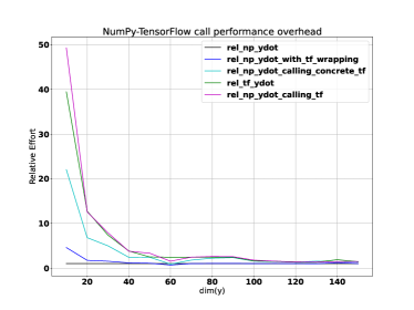
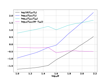
Figure 2: Left: Computational latency for evaluating a function that computes a einsum(’abc,b,c->a’, coeffs, y, y) tensor product, relative to a NumPy-only Python function. Curve rel_np_ydot is constant at 1, rel_np_ydot_with_tf_wrapping includes the effort to convert a numpy.ndarray to a tf.Tensor and back. Curve rel_np_ydot_calling_concrete_tf shows relative effort for calling the ‘concrete TensorFlow function’ for the given input-signature. Curve rel_tf_ydot shows time for TensorFlow to compute a tf.Tensor result from a constant tf.Tensor input. Curve rel_np_ydot_calling_tf shows relative effort for calling a just-in-time-compiled @tf.function-decorated function tf_f not-first-time via tf_f(tf.constant(data, dtype=tf.float64)).numpy(). This in particular includes the effort to determine (through Python-level code) the specific compiled realization from the call-signature. Clearly, for small vector-sizes, the overhead can be very sizeable. Right: $\log_{10}(\mbox{effort-ratio})$/$\log_{10}(\mbox{time / reference\_time})$ log/log-plot for computing the Hessian via methods ‘BP2’ and ‘DP’. Reference time $T_{0}$ is computation of a Hessian via method ‘DP’ for state vector size 100: The point $(\log_{10}N,0)$ sits on the black curve. As the slope of the black curve indicates, computational effort grows roughly cubically for problem sizes above $N=40$. The ‘BP2’ curve sits about 1.5 units above the ‘DP’ curve, indicating a typical relative-effort factor of about 30 in the range shown here. Overall, while the raw effort-ratio (cyan) grows with increasing problem size, growth is sublinear, as is also indicated when dividing the effort-ratio by the problem size (cyan). This suggests that the effort-ratio should (as expected) approach a constant for much larger problem sizes, when the overhead to forward numerical data between the ODE-integrator and the RM-AD framework is fully amortized.

Overall, we conclude that despite method ‘BP2’ being expected to have asymptotically-same time-complexity (i.e. scaling behavior with problem size) as method ‘DP’ if we consider equally-sized ODE time-steps for fixed step size integrators, its big achilles heel is that a large number of (small) ODE integrations that to be performed, and this can prominently surface any relevant constant-effort function call overhead of evaluating the rate-of-change function (and its derivatives). For not-implausible tool combinations and smallish ODEs, observing a performance-advantage of ‘DP’ over ‘BP2’ by a factor 30 should not come as a surprise. This however may look rather different if highly optimized code can be synthesized that in particular avoids all unnecessary processing.

4 Hand-crafting an “orbit non-closure” Hessian

We want to illustrate some of the subtleties that can arise when hand-backpropagating ODEs to compute Hessians by studying an ‘orbit-nonclosure’ loss. This example illustrates how to address subtleties that arise when an objective function depends on both initial and final state of the ODE-integration.

The idea is that for some dynamical system, such as a collection of planets, the state-of-motion is completely described by a collection of positions and velocities (equivalently, momenta), one per object. We are then asking, for a given time interval $\Delta T$, how large the misalignment is between the state-of-motion vector after ODE-integrating the equations of motion over time-interval $\Delta T$ and the starting state-of-motion. Somewhat unusually, the loss here depends on both the initial- and final-state of ODE-integration, in a non-additive way. Overall, this detail complicates hand-backpropagation, and we will address the need to make the construction’s complexity manageable by introducing an appropriate formalism. This, then, is not tied to backpropagation-of-backpropagation applications, but should be generically useful for reasoning about the ‘wiring’ of complicated field theoretic constructions (including ‘differential programming’).

The code that is published alongside this article  provides a Python reference implementation for the algorithms described in Sections 2.3 and 2.5 in general terms in a form that should admit straightforward implementation in other software frameworks in which there is only limited support for (ODE-)backpropagation.

Using the grammar described in Appendix B, we are given the function ydot that computes the “configuration-space velocity” as a function of configuration-space position. We explore this for autonomous systems, i.e. ydot is time-independent and has signature:

    ydot: ^(y[:]) => [:]

(4.1)

The ODE-integrator ODE computes a final configuration-space position given the velocity-function ydot, the initial configuration-vector y[:], as well as the starting time t0[] and final time t1[] and hence has signature:

    ODE: ^(ydot{}, y[:], t0[], t1[]) => [:]

The ODE-backpropagation transformation OBP turns a function with the signature of ydot, as in Eq. (4), into a velocity-function for the backpropagating ODE-integration. There are multiple ways to write this given the grammar, but the idea likely is most clearly conveyed by this form, where the position-vector slot-name for the ‘doubled’ ODE is also y[:] (to allow forming the doubled-ODE of a doubled-ODE), and the configuration-space dimensionality is dim.

    OBP = ^ (ydot{},
             y[:],
             vy[:] = ydot(y[:]=y[:dim]),
             J_ydot[:, :] = ydot(y[:]=y[:dim])[:, d y[:]]) ->
           &concat(0, vy[:], &es(-J_ydot[:, :] @ i, j; y[dim:] @ i -> j))

(4.2)

According to the language rules in appendix B, we can alternatively regard OBP as a higher order function that maps a function-parameter named ‘ydot‘ to a function of a configuration space position ‘y[:]‘, hence another function with the signature of ‘ydot‘, but for the twice-as-wide vector, incorporating also the costate equation.

For the example problem of orbit non-closure, we need a ‘target’ function that measures the deviation between configuration space positions. We will subsequently evaluate this on the initial and final state of ODE-integration for a given time interval and initial position, but the most straightforward “L2 loss” target function one can use here is:

    T = ^(pos0[:], pos1[:],
          delta[:] = pos0[:] - pos1[:]) ->
        &es(delta[:] @ a; delta[:] @ a ->)

(4.3)

It makes sense to introduce names for the first and second derivatives of T:

    T0 = ^(pos0[:], pos1[:]) -> T(pos0[:]=pos0[:],pos1[:]=pos1[:])[d pos0[:]]
    T1 = ^(pos0[:], pos1[:]) -> T(pos0[:]=pos0[:], pos1[:]=pos1[:])[d pos1[:]]
    T00 = ^(pos0[:], pos1[:]) -> T0(pos0[:]=pos0[:], pos1[:]=pos1[:])[:, d pos0[:]]
    T01 = ^(pos0[:], pos1[:]) -> T0(pos0[:]=pos0[:], pos1[:]=pos1[:])[:, d pos1[:]]
    T11 = ^(pos0[:], pos1[:]) -> T1(pos0[:]=pos0[:], pos1[:]=pos1[:])[:, d pos1[:]]

(4.4)

With these ingredients, we can formulate orbit non-closure NC as a function of the velocity-function, initial configuration-vector, and orbit-time as follows:

    NC = ^(ydot{}, y_start[:], t_final[],
           y_final[:] = ODE(ydot{}=ydot, y[:]=y_start[:],
                            t0[]=0, t1[]=t_final[])[:]) ->
         T(pos0[:]=y_start[:], pos1[:]=y_final[:])[]

(4.5)

The gradient of this orbit non-closure with respect to the initial position, which we would write as:

    grad_NC = ^(ydot{}, y_start[:], t_final[]) ->
              NC(ydot{}=ydot, y_start[:]=y_start[:],
                 t_final[]=t_final[])[d y_start[:]]

(4.6)

clearly is useful for finding closed orbits via numerical minimization, and in case the original ODE is well-behaved under time-reversal, this can be computed as follows:

    grad_NC = ^(
      ydot{}, y_start[:], t_final[],
      y_final[:] = ODE(ydot{}=ydot, y[:]=y_start[:], t0[]=0, t1[]=t_final[])[:],
      s_T_y_start[:] = T(pos0[:]=y_start[:], pos1[:]=y_final[:])[d pos0[:]],
      s_T_y_final[:] = T(pos0[:]=y_start[:], pos1[:]=y_final[:])[d pos1[:]],
      s_T_y_start_via_y_final[:] = ODE(ydot{}=OBP(ydot{}=ydot),
                                       y[:]=&concat(0, y_final[:], s_T_y_final[:]),
                                       t0[]=t_final[], t1[]=0)[dim:]) ->
      s_T_y_start[:] + s_T_y_start_via_y_final[:]

(4.7)

The task at hand is now about computing the gradient (per-component, so Jacobian) of grad_NC with respect to y_start[:],

    hessian_NC = ^(ydot{}, y_start[:], t_final[]) ->
                  NC(ydot{}=ydot, y_start[:]=y_start[:],
                     t_final[]=t_final[])[d y_start[:], d y_start[:]]

(4.8)

which is the same as

    hessian_NC = ^(ydot{}, y_start[:], t_final[]) ->
                  grad_NC(ydot{}=ydot, y_start[:]=y_start[:],
                           t_final[]=t_final[])[:, d y_start[:]]

(4.9)

Let us consider a fixed component of grad_NC. Let j henceforth be the index of this component. We first proceed by introducing the following auxiliary vector-valued function S_fn, which computes the sensitivity of the grad_NC[j] component with respect to the starting position of the ODE-integration for s_T_y_start_via_y_final[:] in Eq. (4). We can now write this as:

    S_fn = ^(
      ydot{}, y_start[:], t_final[],
      y_final[:] = ODE(ydot{}=ydot, y[:]=y_start[:],
                       t0[]=0, t1[]=t_final[])[:],
      s_T_y_final[:] = T1(pos0[:]=y_start[:], pos1[:]=y_final[:])[:]) ->
         ODE(ydot{}=OBP(ydot{}=ydot),
             y[:]=&concat(0, y_final[:], s_T_y_final[:]),
             t0[]=t_final[], t1[]=0)[dim:][j, d y[:]]

(4.10)

Using ODE backpropagation again to obtain the gradient, and remembering that we can regard taking the $j$-th vector component as a scalar product with a one-hot vector, i.e.

    x[j] = &es(x[:] @ k; &onehot(j, dim) @ k ->)

we can compute (4) as:

    S_fn = ^ (
      ydot{}, y_start[:], t_final[],
      y_final[:] = ODE(ydot{}=ydot, y[:]=y_start[:], t0[]=0, t1[]=t_final[])[:],
      s_T_y_final[:] = T1(pos0[:]=y_start[:], pos1[:]=y_final[:])[:],
      ydot2{} = OBP(ydot{}=ydot),
      obp1_start[:] = &concat(0, y_final[:], s_T_y_final[:])[:],
      s_T_y_start_via_y_final_ext[:] = ODE(ydot{}=ydot2,
                                           y[:]=obp1_start[:],
                                           t0[]=t_final[], t1[]=0)[:] ) ->
        ODE(ydot{}=OBP(ydot{}=ydot2),
            t0[]=t_final[], t1[]=0,
            y[:]=&concat(0,
                         s_T_y_start_via_y_final_ext[:],
                         &onehot(dim + j, 2 * dim)))

(4.11)

Here, unlike in the initial version of S_fn, we have not trimmed s_T_y_final to its second half, to show more clearly the conceptual form of this 2nd backpropagation approach.

At this point, we encounter a relevant detail: the second ODE(...) starts from an initial position that contains the reconstructed starting-position of the system y_start[:] obtained after numerically going once forward and once backward through ODE-integration. This is exactly the code that an algorithm which provides backpropagation as a code transformation would synthesize here. Pondering the structure of the problem, we can however eliminate some numerical noise by instead starting from the known good starting position, i.e. performing the second ODE-backpropagation as follows:

    ODE(ydot{}=OBP(ydot{}=ydot2),
        t0[]=t_final[], t1[]=0,
        y[:]=&concat(0,
                     y_start[:],
                     s_T_y_start_via_y_final_ext[dim:],
                     &zeros(dim),
                     &onehot(j, dim)))

(4.12)

Now, with S_fn, we have the sensitivity of an entry of the orbit-nonclosure gradient on the initial state of the ODE-backpropagation in Eq. (4). At this point, it might be somewhat difficult to see what to do when not having a formalism that helps reasoning this out, but going back to Eq. 4, it is clear where we are: we need to find the sensitivity of gradNC[j] on the input that goes into T0 and T1.

Once we have these sensitivities of the $j$-th entry of the gradient on y_start[:] and y_final[:] via the pos0[:] respectively pos1[:] slots of T0, T1, we can backpropagate the sensitivity on y_final[:] into an extra contribution to the full sensitivity on y_start[:].

With this insight, we are ready to complete the construction, obtaining the $j$-th row of the Hessian now as follows. We use the prefix s_ as before to indicate the sensitivity of the value of the target function T[] on various intermediate quantities, and the prefix z_ to indicate the sensitivity of gradNC[j] on some specific intermediate quantity. Comments F{nn} label the forward-computation steps, and on the backward pass label reference these forward-labels to flag up the use of an intermediate quantity that produces a contribution to the sensitivity.

    hessian_row_j = ^(
      ydot{}, y_start[:], t_final[],  # F1
      y_final[:] = ODE(ydot{}=ydot, # F2
                       y[:]=y_start[:],
                       t0[]=0,
                       t1[]=t_final[])[:],
      # Value for which we obtain the Hessian - not needed here:
      # T_val = T(pos0[:]=y_start[:], pos1[:]=y_end[:])
      s_T_y_start[:] = T0(pos0[:]=y_start[:], pos1[:]=y_final[:]),  # F3
      s_T_y_final[:] = T1(pos0[:]=y_start[:], pos1[:]=y_final[:]),  # F4
      obp1_start[:] = &concat(0, y_final[:], s_T_y_final[:])[:],  # F5
      ydot2{} = OBP(ydot{}=ydot),
      s_T_y_start_via_y_final[:] = ODE(ydot{}=ydot2, # F6
                                       y[:]=obp1_start,
                                       t0[]=t_final[], t1[]=0)[dim:],
      # The j-th entry of the gradient of T_val.
      # Not needed, but shown to document structural dependency.
      # grad_T_val_entry_j[] = (
      #  [s_T_y_start[:] + s_T_y_start_via_y_final[:]][j]),  # F7
      onehot_j[:] = &onehot(j, dim),
      # We want to know the sensitivity of grad_T_val_entry_j[] on
      # y0. Subsequently, let zj_{X} be the sensitivity of this quantity
      # on the corresponding intermediate quantity {X}.
      # Processing dependencies of intermediate quantities in reverse,
      # obp1_start, then s_T_y_final, s_T_y_start, finally y_final:
      z_obp1_start = ODE(ydot{}=OBP(ydot{}=ydot2),
                         y[:]=&concat(0,
                                      y_start[:],
                                      s_T_y_start_via_y_final[:],
                                      &zeros(dim),
                                      onehot_j))[2*dim:],
      z_s_T_y_final[:] = z_obp1_start[dim:],  # from F5
      z_s_T_y_start[:] = onehot_j[:],  # from F7
      z_y_final[:] = (
        # from F5
        z_obp1_start[:dim] +
        # from F4
        &es(T11(pos0[:]=y_start[:], pos1[:]=y_final[:]) @ a, b;
            z_s_T_y_final[:] @ b -> a) +
        # from F3
        &es(T01(pos0[:]=y_start[:], pos1[:]=y_final[:]) @ a, b;
            z_s_T_y_start[:] @ b -> a))
      ) ->
      # The result is "z_y_start[:]", i.e. grad_T_val[j, d y_start[:]].
      ( # from F3
        &es(T00(pos0[:]=y_start[:], pos1[:]=y_final[:]) @ a, b;
            z_s_T_y_start @ a -> b) +
        # from F4
        &es(T01(pos0[:]=y_start[:], pos1[:]=y_final[:]) @ a, b;
             z_s_T_y_start @ a -> b) +
        # from F2
        ODE(ydot{}=ydot2,
            y[:]=&concat(0, y_final[:], z_y_final[:])[:],
            t0[]=t_final[],
            t1[]=0)[dim:])

(4.13)

We can then readily stack these Hessian-rows into the Hessian $h_{jk}$. Overall, while the Hessian always is a symmetric matrix, this numerical approach gives us a result that is not symmetric-by-construction, and numerical inaccuracies might actually make $h_{jk}\neq h_{kj}$. The magnitude of asymmetric part can be regarded as providing an indication of the accuracy of the result, and one would in general want to project to the symmetric part.

5 Hessians for ODEs – examples

In this Section we apply the backpropagation of gradients and Hessians, as developed in Section 4, through ODEs describing specific dynamical systems of interest. We focus on Hamiltonian systems, where the time-evolution for each component of phase-space is given by a first-order ODE in wall-time. More precisely, we consider Hamiltonian functions H{} with signature

    H: ^(y[:]) => []

(5.1)

where y[:] is a d+d-dimensional phase space vector, which should be treated as the concatenation of the position d-vector and the conjugate momentum d-vector:

    y[:] = &concat(0, q[:], p[:])

(5.2)

Given such Hamiltonian function, the time-evolution ODE of y[:] is given by Hamilton’s equations as

    ydot_H = ^(y[:], q[:]=y[:d], p[:]=y[d:])
               -> &concat(0, H[d q[:]], -H[d p[:]])[:]

(5.3)

In this Section, the Hamiltonian function H{} will successively be taken to be that of the 3d isotropic harmonic oscillator, the Kepler problem, and the 2d three-body-problem. In each case, the loss function NC{} is defined in Eq. (4), Eq. (4), to be the squared-coordinate-distance misalignment between an initial configuration y_start[:] at an initial time (that we fix to 0) and the corresponding time-evolved end-state configuration y_final[:] at boundary time t1[]. For convenience, we copy it here:

    NC = ^(ydot{}, y_start[:], t_final[],
           y_final[:] = ODE(ydot{}=ydot, y[:]=y_start[:],
                            t0[]=0, t1[]=t_final[])[:])
                     ->
                     T(pos0[:]=y_start[:], pos2[:]=y_final[:])[]

(5.4)

where

    T = ^(pos0[:], pos1[:],
          delta[:] = pos0[:] - pos1[:]) ->
        &es(delta[:] @ a; delta[:] @ a ->)

(5.5)

For a given Hamiltonian system as in Eq. (5), the initial configurations of interest on these systems are configurations y_start[:]=Y0[:] with fixed boundary time t1[]=T_final[] corresponding to closed orbits. For a given t1[]=T_final[], we refer to Y0[:] as a solution. Our exact task here is then to perform (using our backpropagation formalism) the evaluation of the loss function, its gradient function and Hessian functions on such solutions. That is, we wish to compute:

    # 0-index loss
    loss = NC(ydot{}=ydot_H, y_start[:]=Y0[:],
              t_final[]=T_final)
    # 1-index gradient
    grad = grad_NC(ydot{}=ydot_H, y_start[:]=Y0[:],
                   t_final[]=T_final)
    # 2-index Hessian
    hessian = hessian_NC(ydot{}=ydot_H, y_start[:]=Y0[:],
                         t_final[]=T_final)

(5.6)

If y_start[:]=Y0[:] with t1[]=T_final[] is indeed a solution, then the loss should be zero. If the solution is stationary, we also expect the gradient-vector-function to evaluate to the zero-vector. Finally, by analyzing the flat directions of the Hessian, we comment on the symmetries of the solution. These are all independent deformations of an orbit-closing solution Y0[:] -> Y0_def[:], such that Y0_def[:] is also an orbit-closing solution for the prescribed orbit-time.

Continuous-parameter symmetries that act on phase-space in a way that commutes with time-translation, i.e. the action of the Hamiltonian, will neither affect time-to-orbit nor orbit-closure. Hence, their infinitesimal action-at-a-point belongs to the nullspace of the Hessian of the aforementioned function, evaluated at that point. It can however happen that a Hessian’s nullspace is larger than deformations that correspond to symmetries of the system. This can happen for different reasons: there can be deformations that do not affect orbit-closure and also time-to-orbit, but nevertheless change the total energy, i.e. the value of the Hamiltonian, or the higher (e.g. fourth) order corrections from the Taylor expansion of the loss function might not respect the symmetry of the system.

Hence, the dynamical symmetries of the Hamiltonian always form a (not necessarily proper) subspace of the symmetries of a solution that leave orbit-time invariant.

5.1 The 3d Harmonic Oscillator

As a first simple example, consider the classical isotropic 3d harmonic oscillator.

The harmonic oscillator describes the dynamics of a point mass m[] in three-dimensional space, experiencing a force towards the coordinate-origin that is proportional to its distance from that point, with spring constant k[]. A generic state-vector y[:] is the concatenation of the six phase space coordinates contained in q[:] and p[:], which respectively correspond to position and conjugate momentum vectors of the mass. For simplicity we set the mass and spring constant to unity. The Hamiltonian function for this system is then

    H_ho3 = ^ (y[:]) ->  (1/2) * &es(y[:3] @ qi; y[:3] @ qi ->)
                      +  (1/2) * &es(y[3:] @ pi; y[3:] @ pi ->)

(5.7)

The rate-of-change function for a phase-space vector y[:] in this system is given by Hamilton’s equations (5) as

    ydot_ho3 = ^(y[:]) -> &concat(0, y[3:], -y[:3])[:]

(5.8)

We now come to the task of evaluating for the harmonic oscillator Eq. (5.1) the loss function Eq. (5), its gradient function and its Hessian functions. As discussed in the introduction of this Section, we choose a particular initial configuration y_start[:]=Y0[:] and fixed boundary time t_final[]=T_final[] such that the corresponding trajectory is a closed orbit. In the harmonic oscillator, such configurations are simply obtained by setting T_final[] to be the “orbit time”, which is a function of the mass and spring constant only, $T=2\pi\sqrt{m/k}$. For this choice of boundary time, any initial state vector yields an orbit. For m[] = k[] = 1, we hence have:

    T_final[] = 6.28318530718  # 2 pi

(5.9)

The arbitrary initial configuration Y0[:] is chosen as

    Y0[:] = [50., 10., 50., -20., 10., -0.1]

(5.10)

We now have all the data to perform an evaluation the loss, gradient and Hessian functions. The loss and its gradient for y_start[:]=Y0[:] and t1[]=T_final[] given in Eq. (5.1) are indeed numerically-zero:

    NC(ydot{}=ydot_ho3, y_start[:]=Y0[:], t_final[]=T_final[])[]
    # = 1.0523667647935759e-17

    grad_NC(ydot{}=ydot_ho3, y_start[:]=Y0[:],
            t_final[]=T_final[])[:]
    #    = [1.22409460e-09, -9.60937996e-10, -4.89819740e-10,
    #       4.50560833e-09, 7.61573915e-10,  4.30725394e-09]

(5.11)

The vector of eigenvalues of the Hessian also has numerically-zero entries:

    &eigvals(hessian_NC(ydot{}=ydot_ho3, y_start[:]=Y0[:],
             t_final[]=T_final[])[:,:])[:]
    #   = [-5.9e-11, -5.9e-11, -5.9e-11,
    #      4.4e-11, 4.4e-11, 4.4e-11]

(5.12)

The zero loss and gradient in Eq. (5.1) indicates that the initial configuration Eq. (5.1) with boundary time Eq. (5.1) is indeed a stable orbit-closure solution for the harmonic oscillator. The zero Hessian eigenvalues (in fact, all entries of the Hessian are zero) captures the fact that with boundary time Eq. (5.1), any arbitrary deformation of Y0[:] preserves orbit closure. It is therefore interesting to note that while the dynamical symmetry group of the Hamiltonian Eq. (5.1) is $U(3)$, the symmetries for orbit closure are in actually $GL(6)$ (i.e. the group of all invertible transformations on the 6-vector Y0[:]). This is then an example of the aforementioned phenomenon that the orbit closure criterion can admit additional symmetries beyond those of the dynamical symmetries of the system. The transformations on phase space associated to these extra symmetries will excite the system to different values for the conserved charges of the Hamiltonian. We will see shortly that, for instance, they may map one orbit-closure solution with energy $E=\texttt{H\_ho3(y[:]=Y0[:])}$ to another orbit-closure solution with energy $E^{\prime}\neq E$.

In Figure LABEL:fig:orbitplots(a), the full line shows the orbit whose initial configuration is the solution Y0[:]. The dotted line shows the trajectory whose initial configuration is a small (and arbitrarily chosen) deformation of Y0[:]:

    Y0_deformed[:] =  [50.70710678 , 10. ,  50. , -20. , 9.29289322,  -0.1]

(5.13)

This trajectory is also an orbit with the same orbit time Eq. (5.1), as expected from the discussion in the prior paragraph. The loss on this deformed solution is

    NC(ydot{}=ydot_ho3, y_start[:]=Y0_deformed[:], t_final[]=T_final[])[]
    #  = 1.0717039249337393e-17

(5.14)

Finally, note that the original solution Y0[:] and the deformed solution Y0_deformed[:] have differing energies, explicitly illustrating the aforementioned situation:

    H_ho3(y[:]=Y0[:]) # = 2800.
    H_ho3(y[:]=Y0_deformed[:]) # = 2828.79

(5.15)

5.2 The 3d Kepler Problem

A more complex system is the 3d Kepler problem. This is the gravitational two-body problem where the central force between the two masses is taken to be proportional to the squared-inverse Euclidean separation. This system is naturally symmetric under three-dimensional spatial translations, and we use this to fix the origin in the centre of mass of the two bodies. This procedure reduces the problem to the motion of one body, with mass equal to the so-called reduced mass mu[] = m1[]*m2[]/(m1[]+m2[]), in a central field with potential energy proportional to the inverse distance of the body to the origin. For simplicity, we also choose the masses m1[], m2[] such that mu[]=1. The Hamiltonian function in terms of a generic phase-space vector

    y[:] = &concat(0, q[:], p[:])[:]

is given, for an appropriately chosen Newton’s constant, as

    H_kepl = ^ (y[:]) -> (1/2) * &es(y[3:] @ i; y[3:] @ i ->)
                               - &pow(&es(y[:3] @ i; y[:3] @ i ->), -1/2)

(5.16)

The rate-of-change vector-function of y[:] is given by Hamilton’s equations as

    ydot_kepl = ^(y[:],
                  r_factor[] = &pow(&es(y[:3] @ i; y[:3] @ i ->), -3/2))
                  -> &concat(0, y[3:], -y[:3] * r_factor[])

(5.17)

As for the prior example (harmonic oscillator), we evaluate the orbit-closure loss function given in Eq. (5), as well as its gradient and Hessian functions, on an orbit-closure configuration (y_start[:]=Y0[:], t1[]=T_final[]). Unlike for the harmonic oscillator, we do not use analytical expressions of the system to ab-initio prescribe a good T_final[] and Y0[:]. Instead, we first fix T_final[] to a sensible value and then let a BFGS optimizer (that minimizes the orbit-closure loss NC{}) find a solution for Y0[:] based on some initialization Y0_init[:]. Note that the BFGS-type optimizers rely on knowing a gradient at each iteration, which we provide by allowing the optimizer to evaluate the grad_NC{} function. Note also that throughout this Section, our optimizer runs are set with target gradient norm tolerance of 1e-12. Now, for the boundary time, we fix

    T_final[] = 6.28318530718

(5.18)

while for the state-vector initialization Y0_init[:], we take

    Y0_init[:] = [0.1, 0.2, -0.33, -0.2, 0.5, -0.1]

(5.19)

After 10 calls of the loss and gradient functions, the optimizer reaches the solution

    Y0[:] = [0.351, 0.706, -1.161, -0.238, 0.595, -0.12]

(5.20)

which one checks corresponds to a bound state (H_kepl(y[:]=Y0[:])[] = -0.5 < 0). We can now evaluate NC{}, grad_NC{}, hessian_NC{} directly on the above solution. For the loss and the gradient, we obtain, respectively:

    NC(ydot{}=ydot_kepl, y_start[:]=Y0[:],
       t_final[]=T_final[])[]
    #  = 8.485708295471493e-19

    grad_NC(ydot{}=ydot_kepl, y_start[:]=Y0[:],
            t_final[]=T_final[])[:]
    #  = [0.0, 0.0, 0.0, 0.0, 0.0, 0.0]

(5.21)

For the Hessian, we obtain the following eigenvalues:

    &eigvals(hessian_NC(ydot{}=ydot_kepl, y_start[:]=Y0[:],
                        t_final[]=T_final[])[:,:])[:]
    #  =  [-2.39514e-07, -1.69088e-07, -8.688e-08,
    #      1.04679e-07, 5.13102e-07, 331.266786046988]

(5.22)

In the above Hessian, we observe five flat directions.

These can be understood as follows: The dynamical symmetries of a bound state of the Kepler problem form a $\mathfrak{so}(4)\simeq\mathfrak{so}(3)\oplus\mathfrak{so}(3)$ Lie algebra, which is six-dimensional. Picking the angular momentum algebra $(L_{x},L_{y},L_{z})$ as an obvious $\mathfrak{so}(3)$ subalgebra, we cannot find three conserved quantities that commute with $\vec{L}$, so the angular momentum subalgebra cannot be a regular subalgebra, it must be a diagonal. Then, the further generators $A_{i}$ must transform nontrivially under the angular momentum algebra. The only option here is that they transform as a vector, i.e. we have $[\vec{L},\vec{L}]\sim\vec{L}$, $[\vec{L},\vec{A}]\sim\vec{A}$. This leaves us with $[\vec{A},\vec{A}]\sim\kappa\vec{L}$, where $\kappa$ provides a sign that depends on the sign of $H$. For bound-states (“planetary orbits”), we get $\mathfrak{so}(4)$ as a symmetry algebra, while for scattering-states (“extrasolar comets”), we get $\mathfrak{so}(3,1)$, with $\mathfrak{iso}(3)$ at-threshold (“parabolic-orbit” bodies). For the Kepler problem, $\vec{A}$ is the Laplace-Runge-Lenz (‘LRL’) vector, which for $k=m=1$ has the form $\vec{p}\times\vec{L}-\vec{r}/r$. Intuitively, the symmetries associated with the components of the LRL vector do not turn circular orbits into circular orbits, but rather change the eccentricity of the orbit. Since they commute with the Hamiltonian, i.e. time-translation, they leave energy, and also orbit-time, invariant. A useful geometrical property here is codified by Kepler’s third law – Orbit-time is is a function of the semimajor axis, i.e. ‘diameter’ of the orbit. For a circular orbit, there is a two-dimensional subspace of eccentricity-inducing/adjusting deformations that leave the orbit-diameter invariant, which can (for example) be parametrized by eccentricity and angular position of the periapsis. The third component of the LRL vector – the one parallel to angular momentum – then acts trivially on the orbiting body’s state-of-motion. The situation parallels the observation that acting with $SO(3)$ on a $3d$ unit-vector will only have two independent $SO(3)$-generators change the vector, while the third (which generates rotations whose axis is aligned with the given vector) acts trivially: In the six-dimensional space of $SO(4)$-generators, we can find a one-dimensional subspace of generators acting one acts trivially on any given motion-state, and the other five give rise to flat directions in the orbit-nonclosure Hessian.

In Figure LABEL:fig:orbitplots(b), the full line shows the orbit whose initial configuration is the solution Y0[:]. We can use an SO(3)-rotation, as allowed by the symmetries of the system (conservation of angular momentum), to rotate Y0[:] into an initial configuration that evolves into an orbit in the (y,z) plane. This is denoted in the figure by the dotted line. The relevant rotation matrix is

    R[:,:] = [[ 0.77615609,  0.40681284,  0.48175205],
              [-0.40681284,  0.90682312, -0.11034105],
              [-0.48175205, -0.11034105,  0.86933297]]

(5.23)

which acts finitely on phase space in the usual way as

    Y0[:] -> Y0_deformed[:] :=
      &concat(0, &es(R[:,:] @ i, j; Y0[:3] @ j -> i),
                 &es(R[:,:] @ i, j; Y0[3:] @ j -> i))
    #  = [1.11022302e-16, 6.25127871e-01, -1.25656979e+00,
    #     0.00000000e+00, 6.49574734e-01, -5.55264728e-02]

(5.24)

The loss on this configuration is

    NC(ydot{}=ydot_ho3, y_start[:]=Y0_deformed[:], t_final[]=T_final[])[]
    #  = 2.916662688870734e-16

(5.25)

5.3 The planar three-body-problem

Our final example is the three-body-problem, restricted to motion in two dimensions. We here use the common abbreviation ‘p3bp’ for the planar three-body problem. For simplicity, we consider units masses and unit Newton’s constant. We first focus on the well-known figure-of-eight orbit-closure solution [27, 28]. We subsequently perform a deformation of this solution along a flat direction of its Hessian, which yields another orbit of the type discovered and analyzed in [1].

A phase-space vector y[:] is now 12-dimensional: six positions (two coordinates for each of the three masses) and six conjugate momenta (again two coordinates per mass). Hamilton’s equations for this system are:

    ydot_p3bp = ^(
      y[:],
      q[:,:] = &reshape(y[:6], 3, 2),
      dist[:,:,:] = q[:,+,:] - q[+,:,:], # dist[i,j,:] = q[i,:] - q[j,:]
      r_factor[:,:] = &pow(&es(dist[:,:,:] @ i, j, a;
                               dist[:,:,:] @ i, j, a -> i, j), -3/2))
       -> &concat(0,
            y[6:],  # dq/dt
            dist[1,0,:] * r_factor[1,0] + dist[2,0,:] * r_factor[2,0],
            dist[0,1,:] * r_factor[0,1] + dist[2,1,:] * r_factor[2,1],
            dist[0,2,:] * r_factor[0,2] + dist[1,2,:] * r_factor[1,2])[:]

(5.26)

where the intermediate quantity r_factor[i,j], i,j = 0,1,2 computes the inverse cube of the Euclidean separation between mass i and mass j.

As for the above two examples, our goal is to evaluate the gradient and Hessian functions of the orbit-closure loss function on a closed orbit solution. As discussed above, we aim for the figure-of-eight solution of [27, 28]. We quote the solution as given in the online three-body-problem gallery [29, 30], recently compiled by the authors of [30] (their conventions align with our). The initial vector is given as

    Y0_init[:] = [-1. ,  0. ,  1. ,
                  0. ,  0. ,  0. ,
                  0.347111,  0.532728,  0.347111,
                  0.532728, -0.694222, -1.065456]

(5.27)

The orbit time is quoted as

T_final[] = 6.324449

(5.28)

and we fix it to this value for the remainder of this analysis. Instead of evaluating the loss, gradient and Hessian directly on the configuration in Eq. (5.3), we first substitute it into a BFGS optimizer (in the same way as we did in the Kepler problem). This allows us to flow to a more accurate solution. After typically about 40 function calls, the optimizer returns a solution such as

    Y0[:] = [-9.99845589e-01, -5.69207692e-06,  9.99845620e-01,
             5.70200735e-06, -3.08148821e-08, -9.93042629e-09,
             3.47140692e-01,  5.32768073e-01, 3.47140612e-01,
             5.32768034e-01, -6.94281303e-01, -1.06553611e+00]

(5.29)

with numerically-zero loss, zero gradient, and Hessian eigenvalues given as:

    NC(ydot{}=ydot_p3bp, y_start[:]=Y0[:],
       t_final[]=T_final[])[]
    #  = 4.459981866710229e-19

    grad_NC(ydot{}=ydot_p3bp, y_start[:]=Y0[:],
            t_final[]=T_final[])[:]
    #  = [6.98443059e-10,  8.23949237e-12, -7.23697523e-10,
    #     8.16570974e-12, 2.52579189e-11, -1.64137619e-11,
    #     -1.97349744e-10, -2.79343635e-10, -1.97437565e-10,
    #     -3.26573785e-10,  3.94809824e-10,  6.05863284e-10]


    &eigvals(hessian_NC(ydot{}=ydot_p3bp, y_start[:]=Y0[:],
                      t_final[]=T_final[])[:,:])[:]
    #  = [-2.9436638e-05, -2.214641e-06, 3.956369e-06,
    #     1.3811708e-05, 0.000595885249, 0.009097681599,
    #     11.10411162849, 17.795125948157, 79.997311426776,
    #     79.997322634127, 2626.009830021427, 10534.09893184725]

(5.30)

The Hessian eigenvalues in Eq. (5.3) above suggest that the solution Eq. (5.3) has four flat directions. These may be identified as follows:

• time-translations, i.e. shifting the initial state-vector along the orbit (1 flat direction).

• translations of the system in two spatial directions (2 flat directions).

• SO(2)-rotation of the system in two spatial directions (1 flat direction).

We now discuss a deformation of this solution. For the prior two systems (harmonic oscillator and Kepler problem) recall that the deformations given in Eq. (5.1), EQ. (5.2) of the original solutions Eq. (5.2), Eq. (5.1) were generated by the allowed symmetries of those solutions (a  $GL(6)$ and $SO(3)$ rotation respectively). In this sense, the deformed solutions were equivalent, under symmetry, to the original solutions.

Here, we want to focus attention on a deformation that is not associated with a null-eigenvalue of the Hessian Clearly, such a deformation cannot be symmetry of the problem, and the resulting deformed state-of-motion vector will not correspond to a closed orbit. That being said, we may pick an eigenvector with small associated eigenvalue, so that we do less damage to orbit-closure than other arbitrary deformations of similar magnitude would do. Upon taking this deformation, our approach is then to take the deformed vector as initialization for a BFGS-type optimization step.

Now, from Eq. (5.3), we choose the eigenvector with eigenvalue $\approx 0.00059\ldots$. The associated eigenvector is

    deformation_evec[:] := &e_vec(hessian_NC(ydot{}=ydot_p3bp, y_start[:]=Y0[:],
                                             t_final[]=T_final[])[:,:])[:])[4]
                         = [-0.40539516 , -0.397770681 , 0.105262168 ,
                            0.289586383 , -0.312660227 , 0.0140926167 ,
                            0.241227186 , 0.406375493 , -0.0000000420869 ,
                           -0.0000000636894 , 0.0651632629 , 0.506912208]

(5.31)

We apply a small shift along this direction to Y0[:]:

    Y0[:] -> Y0[:]_deformed_init[:]
                 = Y0[:] - 0.02 * deformation_evec[:]
                 = [-0.9917376858 , 0.0079497215431 , 0.99774037664 ,
                    -0.0057860256527 , 0.0062531737251 , -0.0002818622644 ,
                    0.34231614828 , 0.52464056314 , 0.3471406128417 ,
                    0.5327680352738 , -0.695584568258 , -1.07567435416]

(5.32)

where the magnitude 0.02 of the deformation was chosen by hand. We now pass Y0[:]_deformed_init into the minimizer. This leads to the new solution:

    Y0_deformed[:] = [-1.00149036,  0.00959776,  1.00543596, -0.01484088,
                      0.00831026, 0.00712495,  0.33774162,  0.53113049,
                      0.35292643,  0.53094484, -0.69066805, -1.06207533]

(5.33)

For this solution, the orbit-nonclosure loss is once again numerically-zero:

    NC(ydot{}=ydot_p3bp, y_start[:]=Y0_deformed[:],
       t_final[]=T_final[])[]
                       = 3.834269651089502e-19

(5.34)

In Figure LABEL:fig:orbitplots(c), we show the orbit corresponding to the original Y0[:] solution Eq. (5.3) and the orbit corresponding to the deformed Y0_deformed[:] solution Eq. (5.3). We note that, unlike for the original solution, the deformed solution gives trajectories where each mass moves on a distinct figure-of-eight curve. This class of solutions turns out to be known. Indeed, they are referred to as the “hyperbolic-elliptic companion orbits” of the figure-of-eight orbit, having been discovered and analyzed in detail in work by Simo [1].

See orbit_plots.pdf

6 Conclusion and outlook

The problem of backpropagating Hessians through ODEs involves quite a few subtleties – in general, the preferred choice of approach will depend on characteristics of the problem, such as whether we want a straightforward-to-understand scheme for validating more sophisticated numerical code, whether or not it is feasible to employ some framework that provides backpropagation capabilities, whether there are disadvantages that are related to computing the Hessian all in one go rather than row-by-row, and whether one is interested only in backpropagating a Hessian around a minimum or not. Given that sensitivity backpropagation allows us to compute the gradient of a $\mathbb{R}^{D}\to\mathbb{R}$ scalar function that is defined in terms of an algorithm with a constant-bound effort multiplier $b\leq 8$, as long as we can remember all intermediate quantities, and given also that calculations that involve ODE integration admit forgetting intermediate quantities if the ODE can be reversed in time, it is unsurprising that an gradient of a scalar-valued function involving ODE backpropagation with not remembered intermediate positions can be computed numerically with effort multiplier $B=b+1$ (if using a fixed time step ODE integrator whose computational effort characteristics are easy to reason about), where the $+1$ is due to the need to redo (and backpropagate) the velocity-field evaluation on the backward pass in order to backpropagate also through that, for evaluating the $\sigma_{i}F_{i,k}$-term. Then, using this approach for every component of a gradient to obtain a Hessian, we can naturally expect to be able to work this out with effort-multiplier no more than $B^{2}D$, not remembering intermediate results for ODE-integration.

Each of the major approaches that have this time complexity in principle has some drawbacks, such as: requiring some software framework that cannot be used for the particular case at hand, not automatically using a good starting point, requiring to solve an ODE with $\leq D^{2}$-dimensional state-vector, or, for the particular case of hand-crafting backpropagation-of-backpropagation code, being laborious and easily getting confusing and also not tolerating constant-effort overhead for computing the rate-of-change function (and its derivatives) well due to the large number of ODEs that need to be solved. Pragmatically, one however observes that the ‘differential programming’ approach here is a very strong contender for many real-world problems.

We addressed the point that ‘the wiring might get complicated’ by means of introducing a dedicated formalism. We hope that our thorough discussion of various nontrivial aspects of the problem may provide useful guidance to practitioners encountering such problems across a broad range of fields.

The one aspect of this work that might appear most unfamiliar to a numerical practitioner is the introduction of a formalism to help manage the complexity that often arises when hand-backpropagating code, including a fully-specified Chomsky type-2 grammar. Considering the use case this formalism was designed for, it addresses the problem that stringent equational reasoning should be possible for ‘tensor-field like’ quantities, as well as (potentially higher order) functions involving such fields with complicated interdependencies, and nothing beyond that. This language in itself looks promising for addressing a frequent complaint by newcomers to field theory (including hydrodynamics) literature that ‘too many dependencies are implicitly understood’, and expressions hence often are not really self-contained in the sense of a precise description of the mathematical idea sans extra information of which dependencies were suppressed. Many students first encounter this problem when trying to make sense of the Euler-Lagrange approach to variational calculus, in the form of “$(d/dt)(\partial L/\partial\dot{\vec{q}})=\partial L/\partial\vec{q}$”. One textbook that handles this aspect with a similar emphasis as ours with respect to “precisely describing the wiring” is [31], and in a way, the formalism presented there can be seen as an intellectual precursor of (certainly an inspiration for) our formal language. Overall, there are three major advantages from aligning the formalism with some ingredients taken from the Python programming language, and NumPy: insisting on named function-slots which may be both unbound or bound not only allows good alignment with actual code implementations (making the formalism suitable for code comments), but also does away with the need of any ‘let’-syntax type syntactic sugar that many functional programming languages identified as essentially necessary to facilitate code clarity. Since our formalism has to support general multilinear algebra, we deliberately do away with concepts such as ‘matrices’ and ‘vectors’, which merely are $n=2$ and $n=1$ special cases of $n$-index objects and use an uniform approach.

While we think (and hope) that our proposal to systematically describe field-theoretic constructions of high complexity might be more generally useful, we by no means consider the proposed language as finalized. Overall, future amendments will however not go against the grain of fundamental design principles. The most important principles here are admitting and simplifying use in code-comments, to improve alignment between expressions in research articles and in code, and ‘staying minimalistic’ in the sense of not introducing anything that would introduce unnecessary special cases.

One aspect which we did not at all discuss in this work is in what sense the ability to easily backpropagate Hessians might shed new lights onto path integral based analysis, considering that in both cases, we are often interested in exploring second-order spatial dependencies of some objective function around a ‘classical’ trajectory.

Appendix A Evaluation of $\sigma_{i}F_{i,k}$

Figure 4 shows TensorFlow code that maps a vector-valued TensorFlow function to a corresponding matrix-valued function that evaluates the Jacobian, optionally admitting autograph-transformation of the Python code for generating efficient low-level code. Here, computation of the Jacobian will effectively use backpropagation using, per intermediate quantity, one sensitivity-accumulator per output-vector entry of the backpropagated function. This means that for a $\mathbb{R}^{D}\to\mathbb{R}^{N}$ function $F$, the effort to compute the Jacobian is bounded by $bN$ times the effort to evaluate $F$ (with $b$ as in the main text). In contradistinction, the code shown in figure 5 computes the gradient of a scalar-valued function $\sigma_{j}F_{j}$, where only the $F_{j}$ are position-dependent. This can be accomplished with effort-multiplier $b$.

⬇

_DEFAULT_USE_AUTOGRAPH = True

def maybe_tf_function(use_autograph):

”””Returns␣tf.function␣if␣use_autograph␣is␣true,␣identity␣otherwise.”””

return tf.function if use_autograph else lambda f: f

def tf_jacobian(t_vec_func: Callable[[tf.Tensor], tf.Tensor],

use_autograph=_DEFAULT_USE_AUTOGRAPH) -> Callable[[tf.Tensor],

tf.Tensor]:

”””Maps␣a␣TF␣vector-valued␣function␣to␣its␣TF␣Jacobian-function.”””

# This is here only used to work out the hessian w.r.t. ODE initial-state

# and final-state coordinates.

# (!!!) Computing the costate-equation jacobian with this would be wasteful.

@maybe_tf_function(use_autograph)

def tf_j(t_xs):

tape = tf.GradientTape()

with tape:

tape.watch(t_xs)

v = t_vec_func(t_xs)

ret = tape.jacobian(v, t_xs,

unconnected_gradients=tf.UnconnectedGradients.ZERO)

return ret

return tf_j

Figure 4: Mapping a vector-valued TensorFlow function to a function computing its Jacobian. The unconnected_gradients=tf.UnconnectedGradients.ZERO keyword argument ensures that TensorFlow produces a mathematically correct zero gradient, rather than a None-value if the graph for v is not connected to t_xs.

⬇

def tf_jac_vec_v0(

t_vec_func: Callable[[tf.Tensor], tf.Tensor],

use_autograph=_DEFAULT_USE_AUTOGRAPH) -> Callable[[tf.Tensor, tf.Tensor],

tf.Tensor]:

”””Maps␣a␣TF␣vector-function␣F␣to␣a␣”(x, sx) -> sx_j Fj,k(x)”␣function.”””

@maybe_tf_function(use_autograph)

def tf_j(t_xs, t_s_xs):

tape = tf.GradientTape()

with tape:

tape.watch(t_xs)

t_v = t_vec_func(t_xs)

return tape.gradient(t_v, t_xs,

output_gradients=[t_s_xs],

unconnected_gradients=tf.UnconnectedGradients.ZERO)

return tf_j

def tf_jac_vec_v1(

t_vec_func: Callable[[tf.Tensor], tf.Tensor],

use_autograph=_DEFAULT_USE_AUTOGRAPH) -> Callable[[tf.Tensor, tf.Tensor],

tf.Tensor]:

”””Maps␣a␣TF␣vector-function␣F␣to␣a␣”(x, sx) -> sx_j Fj,k(x)”␣function.”””

@maybe_tf_function(use_autograph)

def tf_j(t_xs, t_s_xs):

tape = tf.GradientTape()

with tape:

tape.watch(t_xs)

t_v = tf.tensordot(t_s_xs, t_vec_func(t_xs), axes=1)

return tape.gradient(t_v, t_xs,

unconnected_gradients=tf.UnconnectedGradients.ZERO)

return tf_j

Figure 5: Mapping a vector-valued TensorFlow function to the gradient of its scalar product with a given vector. This can be accomplished by either using the somewhat under-documented output_gradients= parameter of tf.GradientTape.gradient, or alternatively by taking the partial gradient of a scalar product.

Appendix B A DSL for dependencies in tensor calculus

This appendix describes the notational conventions used in this work in detail. These conventions, which have been designed to simplify equational reasoning about (multi-index) tensor calculus dependencies, can be regarded as a domain specific language (DSL) – henceforth abbreviated ‘TCD-DSL’. They not only should be useful to adapt the reasoning outlined in this work to minor variations such as explicitly time-dependent velocity-functions, but may ultimately (perhaps after some refinement of the grammar) be considered useful more widely for generic vector/tensor calculus problems, not only at the interface of symbolic analysis and numeric computation, but also whenever having a precise specification of the wiring is important.

The incentive for this formal language comes from the need to simplify keeping track of functional dependencies of tensorial quantities in situations where the commonly used formalism that heavily makes use of abuse-of-notation approaches becomes too unwieldy or ambiguous. The grammar proposal presented here is to be seen as a starting point for further discussion, and should not be considered as being cast in stone.

While this article comes with a proper PEG grammar specification [32] with which expressions can be checked (using a parser generator) with respect to grammatical well-formedness, no effort has yet been attempted to implement higher level components of a compiler that can process computational specifications following this grammar into various other forms, including NumPy. Even having only the syntax analysis part of such a compiler fleshed out clearly would be useful for discovering typos in an automated fashion. Still, the structure of the grammar is such that it should allow adding these components in a rather straightforward manner. The TCD-DSL grammar in its present form is presented in appendix C.

B.1 Design desiderata

The fundamental requirements that the language’s design addresses are:

1. The language should be minimalistic, addressing precisely the unavoidable requirements, but with powerful primitives that eliminate the need for complicated structure.

2. The language should rely on tried-and-tested widely understood approaches for the sub-problems it needs to handle: some form of lambda calculus for functional dependencies and function-application, some form of tensor arithmetics to specify complicated tensor contractions and index reshufflings, and NumPy like syntax for common operations on multi-index arrays, such as reshaping, index-expansion, broadcasting, and slicing. This is in particular to simplify aligning formal expressions with code using a NumPy-like approach to handling multi-index data.

3. Expressions should be good to use in textual descriptions, such as research articles, but also admit being added verbatim as explanatory comments to code without requiring the reader to hallucinate the effects of typesetting instructions.

The final requirement here asks for using a plain ASCII-based textual representation, perhaps using indentation for emphasis.

We decided to use an amalgamation of lambda calculus and python/lisp-style multi-parameter keyword arguments, with the character ‘^’ representing the ‘lambda‘ that indicates an “anonymous function”. The second requirement asks for introducing some way to bind functions to names (treating functions as ‘first-class citizens’ in the value-universe) and to represent function-evaluation. In a language like LISP or OCaml, it would not be uncommon to have both a way to specify an anonymous function, such as (lambda (x) (* x x)), and on top of that some syntactic sugar for introducing scoped variable bindings, such as (let ((x-squared (* x x))) {body}), which is semantically equivalent to an immediately-evaluated lambda, such as ((lambda (x-squared) {body}) (* x x)). If we require function parameters to always be named, this allows us to kill three birds with one stone: We get close alignment with a possible translation to code from named-keyword parameters as available in Python (and also LISP), plus a rather intuitive way to specify partial derivatives with respect to parameters, and on top of that can meld let into lambda with one simple convention.

B.2 Concept overview

The main concepts designed into this language are:

• Positionally-indexed multi-index numerical quantities. Alongside function parameter names, the number of indices is generally indicated by square bracket indexing ‘[:, :, ...]’ that would be valid Python syntax and a no-op when applied to a multi-index quantity of the intended shape, and not also valid for some quantity with a different number of indices: While a 3-index numpy array x could be indexed as ‘x[:, :], this would also be valid indexing for a 2-index numpy array. This is not permitted here – if a parameter is designated as x[:,:,:], this clearly specifies that the quantity carries three indices.

• Tensor contractions use an uniform approach that is based on generalized Einstein summation, via a special-function language primitive ‘&es()’. While this is slightly burdensome for simple scalar products and matrix/vector products, it follows the minimality principle that special cases of fundamental operations should not have special non-uniform syntax. As a consequence of this design, tensor index names (which are ubiquitous in field theory) can only occur to specify how to form and contract products, and outside such ‘&es()’ expressions, indices on tensors are discriminated by index-order alone.

• Immediately-bound function parameters. All function parameters are named, and unlike in pure lambda calculus (but like in most programming languages), functions can have multiple parameters. Borrowing some ideas from modern C++ constructor initialization syntax, named parameters can have a value assigned to them right at the time of their introduction, and this can refer to immediately-bound function parameters that were bound earlier (i.e. to the left of the current argument) on the same evaluation parameter-list. This means that we want to consider this expression, which describes a function with one open named scalar (zero-indices) parameter a that gets mapped to a+a*a

      ^(a[], b[]=a[]*a[]) -> a[] + b[]
  

  (B.1)

  as being equivalent to the expression:

      ^(a[]) -> (^(a[], b[]) -> a[] + b[])(a[]=a[], b[]=a[]*a[])
  

  (B.2)

  The corresponding rules for name-resolution are:

  • If a name ‘x[...]’ is used in an expression, the name this is looked up by going through a sequence of fallbacks, where the first-found binding wins.

  • If the expression is the right hand side of a bound-parameter introduction, the name is looked up first among the earlier-introduced parameters on the same lambda parameter-list, where the latest (rightmost-in-text) such parameter-binding gets checked first.

  • Otherwise, the tightest lexically-surrounding lambda’s parameter bindings, right-to-left, will be checked, then the lexically next outer lambda’s bindings, etc. If no binding is found, the name is considered to be ‘unbound’, so considered as coming from ‘global’ context.

• Partial derivatives. These are expressed by adding an index such as d Z[:] to a positionally-indexed quantity. The semantic meaning of such an index is that, for every combination of the other indices present on the positionally-indexed quantity with this partial-derivative index removed, we use sensitivity backpropagation to determine the sensitivity of the corresponding coefficient on the coefficients of the input parameter named after the ‘d’. If a partial derivative is taken with respect to an immediately-bound multi-index quantity, the corresponding gradient represents the sensitivity (relative to $\varepsilon$, to first order) of the entries of the multi-index quantity without the partial-derivative slot with respect to $\varepsilon$-perturbations of the individual coordinates of the input. When taking partial derivatives with respect to a $k$-index input, this splices k indices into the index list of the designated partial derivative (so, adding zero extra indices for a partial derivative with respect to a scalar).

  Hence,

      ^(x[:], y[:]=x[:]) -> &es(x[:] @ a; y[:] @ a ->)[d y[:]]
  

  (B.3)

  is the derivative of the scalar product of a vector with itself with respect to varying the 2nd factor only. This is equivalent to the eps[i]$\rightarrow 0$ limit of g in:

      f = ^(x[:], y[:]) -> &es(x[:] @ a; y[:] @ a ->)[d y[:]]
      g = ^(x[:]) -> (f(x[:]=x[:], y[:]=x[:]+eps[:]) - f(x[:]=x[:], y[:]=x[:])) / eps[:]
  

  (B.4)

  using NumPy’s broadcasting rules to divide by a vector.

• Identifying a 0-parameter function with its value. We generally consider ^() -> T[:] to be equivalent to T[:] (and likewise for other numbers of indices on the object).

• Functions can take functions as parameters. This is generally indicated by putting curly-braces indexing behind a slot-name. The current form of the grammar makes no attempt to precisely represent the slot-name expectations for such function-parameters.

• The grammar should also have a notion of “whitespace” that admits comments – here in the form of “hash character ‘#’ starts whitespace that ends at end-of-line”.

B.3 Open questions

It has been said that every formal language first and foremost codifies what things its author did not properly understand. Major pain points around the current language proposal which likely would benefit from subsequent refinement include:

• For function-parameters, no detail about their call signature is (or can be) made part of the parameter-specification. This is a trade off between brevity and precision.

• Ultimately, one likely would want to extend the grammar to admit tagging indices that correspond to a particular linear representation of some Lie group group and the representation, such as “this is a SO(3, 1) co-vector index”.

• It is not yet clear what the best style decisions are with respect to proper use of technically unnecessary index-structure specifications. Is it visually clearer to mandate T(pos0[:]=v0[:], pos1[:]=v1[:]), or should the terser form T(pos0[:]=v0, pos1[:]=v1) be given preference?

Appendix C PEG grammar

The PEG grammar for TCD-DSL is listed in this appendix. The grammar rule comments provide additional clarification about specific rules. This grammar can be directly processed by a parser generator such as in particular the ‘lark’ Python module  to produce a working parser. The code published alongside this article provides a corresponding grammar-checker, which can also check expressions in LaTeX files.

⬇

// Valid input consists of zero or more statements.

?start: (signature_spec | statement)*

// A signature-specification.

signature_spec: (NAME ”:”)? LAMBDA lambda_args ”=>” signature_rhs

?signature_rhs: (signature_spec | (”[” (COLON (”,” COLON)*)? ”]”))

// An individual statement is either an expression or a definition.

statement: expr | definition

// A definition is equivalent to a parameter binding.

// The only difference is that definitions are top-level, i.e. not scoped.

definition: parameter_binding

// An expression is a tensorial expression or a function-definition.

?expr: tensor_expr | fn_lambda

// Function, using ”lambda notation”: \(param1[:], param2[:]) -> {expr}

// Clarification: The right hand side expression can indeed

// be a function-definition, indicating a lexical closure.

fn_lambda: LAMBDA lambda_args ”->” expr

// lambda arguments

lambda_args: ”(” (fn_arg (”,” fn_arg)*)? ”)”

// Tensor expression

?tensor_expr: tensor_sum | tensor_optionally_indexed

?tensor_optionally_indexed: tensor_optionally_indexed_head bracketed_indexing*

?tensor_optionally_indexed_head: tensor_paren

| tensor_special_fn

| tensor_atom

// A parenthesized tensor expression may evaluate to a callable,

// so can optionally have call-arguments.

// This is valid:

// ”(\(x[:], y[:]) -> x[0]*y[0])(x[:]=y[:])”

// (”We take a function of two vectors, ‘x‘ and ‘y‘, which computes the

// product of the leading components, and bind the 2nd input to have

// the same value as the first, leaving us with this function:

// ”\(x[:]) -> x[0] * x[0]”.

?tensor_paren: /[+-]/? ”(” expr ”)” call_args*

// Function calls bind zero or more parameters.

// Interpretation: if only some slots are bound, the value of the

// call-expression is the function of the still-to-be-bound named

// parameters. A parameter-binding can refer to another earlier.

// parameter-binding on the same call.

call_args: ”(” (parameter_binding (”,” parameter_binding)*)? ”)”

// A function argument is either a bound or an unbound slot.

fn_arg: slot_spec // Unbound slot.

| parameter_binding // Bound slot.

// Q: Do we handle binding function-slots against functions properly?

parameter_binding: slot_spec ”=” expr

// A tensor sum-expression can start with a sign, and is a sum of one

// or more tensor product-expressions.

?tensor_sum: /[+-]/? tensor_prod (/[+-]/ tensor_prod)*

// A tensor product-expression is a parenthesized or atomic

// tensor-expression, followed by zero or more such expressions

// separated by multiplication or division.

// The operator is made mandatory, since otherwise,

// telling apart a product expression such as ”x[:](y[:]+z[:])”

// from a function-application such as ”x[:](y[:]=z[:])”

// may be visually confusing.

?tensor_prod: tensor_optionally_indexed (/[*\/]/ tensor_optionally_indexed)*

// An atomic tensor expression is either a number or a name,

// optionally to be called, and optionally with indexing.

?tensor_atom: number | NAME call_args*

// Index-names may get extended later to also admit transporting

// information about the group and the representation.

index_name: NAME

index_name_seq: index_name (”,” index_name)*

// ==============

// ”[…]” indexing where individual indices may carry tags such as ”@a”.

bracketed_indexing: ”[” (index (”,” index)*)? ”]”

// An index is either a Python ”start:stop:range” type index, or ”d slot”.

// A ’+’, when used as an index, corresponds to ‘numpy.newindex‘.

// NumPy’s broadcasting rules are understood, except that broadcasting

// always requires both expressions to have the same number of indices,

// and if ranges for some particular index differ, then one of them

// must be a range-1 index.

index: DIFF WS diff_slot_spec

| stride_part? (COLON stride_part?) ~ 0..2

| ”+”

// For ease of changing the definition of some tokens.

DIFF: ”d”

LAMBDA: ”^”

COLON: ”:”

?stride_part: int_expr

// A slot specifier, such as ‘pos0[:]‘ in ODE(pos0[:]=y[:10])

// The only allowed forms are:

// - optional list of comma-separated COLONs in square brackets.

// - literal {} to indicate that we are passing in a function here.

// TODO: When passing in a function, do we need to do something about slot-renaming?

slot_spec: NAME /\{\}/

| diff_slot_spec

?diff_slot_spec: NAME (”[” (COLON (”,” COLON)*)? ”]”)?

// Integer expressions - for indexing.

// Rules parallel the tensor_{paren|sum|prod} rules.

?int_num: /[+-]?[0-9]+/

?int_atom: int_num | /[+-]/? NAME

?int_expr: int_atom | int_paren | int_sum

?int_paren: /[+-]/? ”(” (int_sum | int_paren) ”)”

?int_sum: /[+-]/? int_prod (/[+-]/ int_prod)*

?int_prod: (int_paren | int_atom) (/[*\/]/? (int_paren | int_atom))*

// Tensor special-functions: concatenation, stacking, reshaping,

// and other operations.

// Also: Since all ”field-functions” have all slots named,

// common unnamed-slots functions (like &exp) also will be of

// this type.

// These functions all start with a ’&’.

tensor_special_fn: ”&” any_special_fn

?any_special_fn: special_concat

| special_stack

| special_reshape

| special_onehot

| special_zeros

| special_es

| special_analytic

// Tensor-concatenation special function.

// Leading parameter needs to be a literal integer,

// the axis along which to concatenate.

special_concat: ”concat” ”(” int_num ”,” tensor_expr (”,” tensor_expr)* ”)”

// Stacking. Syntactically equivalent to concatenation.

special_stack: ”stack” ”(” int_num ”,” tensor_expr (”,” tensor_expr)* ”)”

// Reshaping. Indices are to be provided as a list of integers.

special_reshape: ”reshape” ”(” tensor_expr ”,” int_num (”,” int_num)* ”)”

// One-hot. Index and dimension can be int-expressions.

special_onehot: ”onehot” ”(” int_expr ”,” int_expr ”)”

// Vector of zeros.

special_zeros: ”zeros” ”(” (NAME | int_num) ”)”

// Generalized ”Einstein Summation”. This uses rather special syntax.

// - Product-factors are separated with semicolons,

// - Multi-index product-factors are expected to have all indices named

// with ”@ indexname1, indexname2, …”.

// - 0-index (scalar) tensors need not have index names.

// - result-indices are listed after ’->’.

// Interpretation:

// - multi-index array indices are named according to the order in which

// indices occur.

// - Every right hand side index combination addresses one coefficient

// of the resulting tensor (in index order). The left hand side

// indices that do not also occur on the right hand side

// are being summed over. (This ”generalized” Einstein summation is

// group-theoretically unsound, but useful for formulas that are

// ultimately not using group theory, but short-cuts.)

special_es: ”es” ”(” index_named ( ”;” index_named ) * ”->” index_names? ”)”

// Single-argument special-functions,

special_analytic: special_analytic_1arg | special_analytic_2arg | special_matrix

// For mult-index tensorial quantities, these are understood to operate

// element-wise on the coordinates.

?special_analytic_1arg: (”exp” | ”log”) ”(” tensor_expr ”)”

?special_analytic_2arg: ”pow” ”(” tensor_expr ”,” tensor_expr ”)”

// Eigenvalues/Eigenvectors, 2-index-to-1-index or 2-index-to-2-index:

?special_matrix: (”eigvals” | ”eigvecs”) ”(” tensor_expr ”)”

index_named: tensor_expr (”@” index_names?)?

index_names: index_name (”,” index_name)*

NAME: /[A-Za-z][A-Za-z0-9_]*/

// TODO: This needs further refinement.

number: /[0-9]+/

// Whitespace – will get ignored.

WS: /(\s|#.*)+/

%ignore WS

References

- [1] Carles Simó. Dynamical properties of the figure eight solution of the. In Celestial Mechanics: Dedicated to Donald Saari for His 60th Birthday: Proceedings of an International Conference on Celestial Mechanics, December 15-19, 1999, Northwestern University, Evanston, Illinois, volume 292, page 209. American Mathematical Soc., 2002.
- [2] William H Press, Saul A Teukolsky, William T Vetterling, and Brian P Flannery. Numerical recipes 3rd edition: The art of scientific computing. Cambridge university press, 2007.
- [3] Seppo Linnainmaa. Taylor expansion of the accumulated rounding error. BIT Numerical Mathematics, 16(2):146–160, 1976.
- [4] Bert Speelpenning. Compiling fast partial derivatives of functions given by algorithms. University of Illinois at Urbana-Champaign, 1980.
- [5] David E Rumelhart, Geoffrey E Hinton, and Ronald J Williams. Learning representations by back-propagating errors. nature, 323(6088):533–536, 1986.
- [6] Sepp Hochreiter and Jürgen Schmidhuber. Long short-term memory. Neural computation, 9(8):1735–1780, 1997.
- [7] Geoffrey E Hinton, Simon Osindero, and Yee-Whye Teh. A fast learning algorithm for deep belief nets. Neural computation, 18(7):1527–1554, 2006.
- [8] Kaiming He, Xiangyu Zhang, Shaoqing Ren, and Jian Sun. Deep residual learning for image recognition. In Proceedings of the IEEE conference on computer vision and pattern recognition, pages 770–778, 2016.
- [9] Ricky TQ Chen, Yulia Rubanova, Jesse Bettencourt, and David K Duvenaud. Neural ordinary differential equations. Advances in neural information processing systems, 31, 2018.
- [10] Amir Gholami, Kurt Keutzer, and George Biros. Anode: Unconditionally accurate memory-efficient gradients for neural odes. arXiv preprint arXiv:1902.10298, 2019.
- [11] Revaz V Gamkrelidze. Discovery of the maximum principle. Journal of dynamical and control systems, 5(4):437–451, 1999.
- [12] Thomas Fischbacher. A rosetta stone for subproblem optimality. In Preparation.
- [13] Guan-Horng Liu, Tianrong Chen, and Evangelos Theodorou. Second-order neural ode optimizer. Advances in Neural Information Processing Systems, 34:25267–25279, 2021.
- [14] Martín Abadi, Ashish Agarwal, Paul Barham, Eugene Brevdo, Zhifeng Chen, Craig Citro, Greg S. Corrado, Andy Davis, Jeffrey Dean, Matthieu Devin, Sanjay Ghemawat, Ian Goodfellow, Andrew Harp, Geoffrey Irving, Michael Isard, Yangqing Jia, Rafal Jozefowicz, Lukasz Kaiser, Manjunath Kudlur, Josh Levenberg, Dandelion Mané, Rajat Monga, Sherry Moore, Derek Murray, Chris Olah, Mike Schuster, Jonathon Shlens, Benoit Steiner, Ilya Sutskever, Kunal Talwar, Paul Tucker, Vincent Vanhoucke, Vijay Vasudevan, Fernanda Viégas, Oriol Vinyals, Pete Warden, Martin Wattenberg, Martin Wicke, Yuan Yu, and Xiaoqiang Zheng. TensorFlow: Large-scale machine learning on heterogeneous systems, 2015. Software available from tensorflow.org.
- [15] Adam Paszke, Sam Gross, Francisco Massa, Adam Lerer, James Bradbury, Gregory Chanan, Trevor Killeen, Zeming Lin, Natalia Gimelshein, Luca Antiga, et al. Pytorch: An imperative style, high-performance deep learning library. Advances in neural information processing systems, 32, 2019.
- [16] James Bradbury, Roy Frostig, Peter Hawkins, Matthew James Johnson, Chris Leary, Dougal Maclaurin, George Necula, Adam Paszke, Jake VanderPlas, Skye Wanderman-Milne, and Qiao Zhang. JAX: composable transformations of Python+NumPy programs, 2018.
- [17] Tianqi Chen, Mu Li, Yutian Li, Min Lin, Naiyan Wang, Minjie Wang, Tianjun Xiao, Bing Xu, Chiyuan Zhang, and Zheng Zhang. Mxnet: A flexible and efficient machine learning library for heterogeneous distributed systems. arXiv preprint arXiv:1512.01274, 2015.
- [18] Yuanming Hu, Luke Anderson, Tzu-Mao Li, Qi Sun, Nathan Carr, Jonathan Ragan-Kelley, and Frédo Durand. Difftaichi: Differentiable programming for physical simulation. arXiv preprint arXiv:1910.00935, 2019.
- [19] Stephen Wolfram. The mathematica book, volume 1. Wolfram Research, Inc., 2003.
- [20] André Heck and Wolfram Koepf. Introduction to MAPLE, volume 1993. Springer, 1993.
- [21] Scott D Cohen, Alan C Hindmarsh, and Paul F Dubois. Cvode, a stiff/nonstiff ode solver in c. Computers in physics, 10(2):138–143, 1996.
- [22] Dong C Liu and Jorge Nocedal. On the limited memory bfgs method for large scale optimization. Mathematical programming, 45(1):503–528, 1989.
- [23] Stanley D Deser and Bruno Zumino. Consistent supergravity. Phys. Lett. B, 62(CERN-TH-2164):335–337, 1976.
- [24] Daniel Z Freedman, P van Nieuwenhuizen, and Sergio Ferrara. Progress toward a theory of supergravity. In Supergravities in Diverse Dimensions: Commentary and Reprints (In 2 Volumes), pages 512–516. World Scientific, 1989.
- [25] Daniel Z Freedman and Antoine Van Proeyen. Supergravity. Cambridge university press, 2012.
- [26] Fredrik Johansson et al. mpmath: a python library for arbitrary-precision floating-point arithmetic (version 0.18). Official Wiki Page available at: http://code. google. com/p/mpmath, 2013.
- [27] Alain Chenciner and Richard Montgomery. A remarkable periodic solution of the three-body problem in the case of equal masses. Annals of Mathematics, pages 881–901, 2000.
- [28] Cristopher Moore. Braids in classical dynamics. Physical Review Letters, 70(24):3675, 1993.
- [29] Milovan Šuvakov and Veljko Dmitrašinović. Three-body gallery.
- [30] Milovan Šuvakov and Veljko Dmitrašinović. Three classes of newtonian three-body planar periodic orbits. Physical review letters, 110(11):114301, 2013.
- [31] Gerald Jay Sussman and Jack Wisdom. Structure and interpretation of classical mechanics. The MIT Press, 2015.
- [32] Bryan Ford. Parsing expression grammars: a recognition-based syntactic foundation. In Proceedings of the 31st ACM SIGPLAN-SIGACT symposium on Principles of programming languages, pages 111–122, 2004.