Stable Contact Guaranteeing Motion/Force Control
for an Aerial Manipulator on an Arbitrarily Tilted Surface

Abstract

This study aims to design a motion/force controller for an aerial manipulator which guarantees the tracking of time-varying motion/force trajectories as well as the stability during the transition between free and contact motions. To this end, we model the force exerted on the end-effector as the Kelvin-Voigt linear model and estimate its parameters by recursive least-squares estimator. Then, the gains of the disturbance-observer (DOB)-based motion/force controller are calculated based on the stability conditions considering both the model uncertainties in the dynamic equation and switching between the free and contact motions. To validate the proposed controller, we conducted the time-varying motion/force tracking experiments with different approach speeds and orientations of the surface. The results show that our controller enables the aerial manipulator to track the time-varying motion/force trajectories.

I INTRODUCTION

Unmanned aerial manipulators (UAMs) interacting with structures located in hard-to-reach areas (e.g., walls or windows installed on tall structures) has been one of the most popular research topics in aerial robotics. Such tasks include window-cleaning [1], painting [2], and non-destructive inspection [3], and there needs a motion/force controller for operations with higher precision. Particularly, for the tasks such as teleoperation [4], multi-manual object manipulation [5] and plug-pulling [6], the capability to track the time-varying motion/force trajectories is also required. However, very few studies have designed a time-varying motion/force tracking controller which simultaneously considers model uncertainty and switching between the free and contact motion.

In [7], [8] and [9], motion/force controllers for the omnidirectional aerial vehicles equipped with a robotic arm were proposed. However, since we are more interested in utilizing a conventional underactuated multirotor rather than developing a special configuration for an omnidirectional aerial vehicle, we focus on designing a motion/force controller for an underactuated UAM (uUAM) configured with an underactuated multirotor and a robotic arm.

An impedance-based force controller was presented in [10] and [11] for a uUAM conducting peg-in-hole insertion tasks. In [12], an image-based visual impedance force controller was introduced. However, those controllers were designed under the assumption that the desired force is constant. Also, [13] proposed a contact force tracking controller minimizing the battery consumption, and [14] introduced a nonlinear motion/force model predictive controller. However, they only conducted tracking experiments for constant force. Although the tracking of time-varying force was conducted in [15], [16] and [17], they did not prove the stability under the model uncertainty and switching behavior between the free and contact motion.

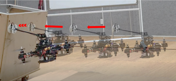
Figure 1: An aerial manipulator approaches a tilted surface and tracks the desired motion and force trajectories while maintaining stable contact.

In this paper, we present a motion/force controller for a uUAM which guarantees both the tracking of time-varying motion/force trajectories and stability during the transition between the free and contact motions. To this end, we derive the translational dynamic model of the uUAM exerting force on a tilted surface with respect to the position of the end-effector, and model the force as the Kelvin-Voigt linear model. Also, a disturbance-observer (DOB)-based motion/force controller is designed, and its gains are calculated to satisfy the analytically obtained input-to-state stability conditions, considering the model uncertainty as well as the switching between the free and contact motions. To validate the proposed controller, we conduct time-varying force-tracking experiments on a tilted surface with a coaxial octocopter-based aerial manipulator with different approach speeds as shown in Fig. 1.

This paper is outlined as follows; In Section II, we formulate the translational dynamic model of a uUAM exerting force to a tilted surface, and we describe the planning and control strategies for motion/force tracking in Section III. In Section IV, we present a scheduling procedure of the controller gains which are utilized during the contact motion, and the proposed controller is validated experimentally in Section V.

Notations: 0_ij, $I_{i}$ and $e_{3}$ represent the $i\times j$ zero matrix, $i\times i$ identity matrix and $[0;0;1]$, respectively. For vectors $\alpha$ and $\beta$, we let $\alpha_{i}$ and $[\alpha]_{\times}\in\mathbb{R}^{3\times 3}$ denote the $i$-th element of $\alpha$ and the operator which maps $\alpha$ into a skew-symmetric matrix such as $[\alpha]_{\times}\beta=\alpha\times\beta$, respectively. Also, we abbreviate the phrase ”with respect to” to w.r.t..

II Translational Dynamic Model

II-A Dynamic Equation w.r.t. the Position of the End-Effector

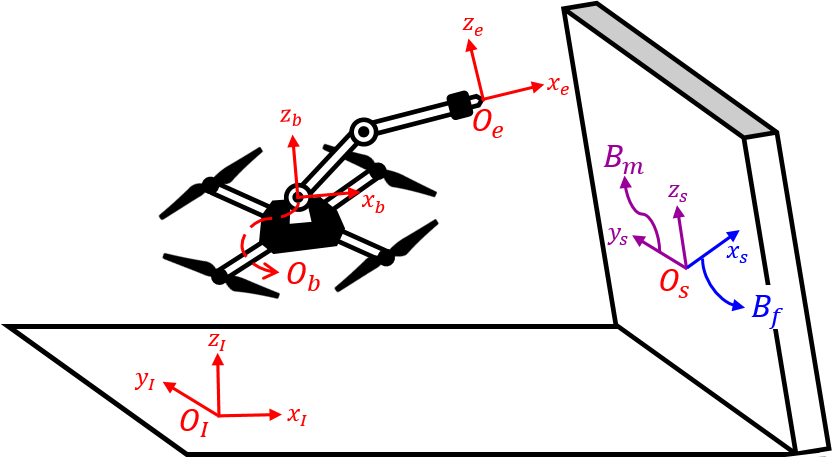
Figure 2: Illustration of a uUAM flying in front of a tilted surface. Coordinate frames required to demonstrate the uUAM system and the basis vectors of force and motion spaces are depicted.

In Fig. 2, coordinate frames to describe the configuration of the uUAM and the tilted surface are defined. Let $O_{I}$, $O_{b}$ and $O_{e}$ denote the inertial, multirotor body and end-effector coordinate frames, respectively, and $O_{s}$ the surface coordinate frame with its $x$ axis aligned with the force exerting direction. The generalized coordinate variables of the uUAM $q\triangleq[p;\phi;\theta]$ is defined with the position of the multirotor in $O_{I}$, $p\triangleq[p_{x};p_{y};p_{z}]$, the Euler angles of the multirotor, $\phi\triangleq[\phi_{x};\phi_{y};\phi_{z}]$, and the joint angles of the robotic arm, $\theta\triangleq[\theta_{1};\cdots;\theta_{n}]$. We set the generalized control input $\tau$ as $[TR(\phi)e_{3};\tau_{\phi};\tau_{\theta}]$ where $T\in\mathbb{R}$, $R(\phi)\in SO(3)$ $\tau_{\phi}\in\mathbb{R}^{3}$ and $\tau_{\theta}\in\mathbb{R}^{n_{a}}$ represent the total thrust of the multirotor, the rotation matrix from $O_{b}$ to $O_{I}$, the body torque in the body frame and the actuator torques of the robotic manipulator, respectively, where $n_{a}$ means the number of actuators used in the robotic arm.

According to [18, Proposition 2] the translational dynamic model w.r.t. the center-of-mass position of a uUAM, $p_{t}$, is expressed as follows:

$$m_{t}\ddot{p}_{t}+m_{t}ge_{3}=TRe_{3}+f_{e}+\delta_{t}$$ (1)

where $m_{t},g\in\mathbb{R}$, $f_{e}$ and $\delta_{t}\in\mathbb{R}^{3}$ express the mass of the uUAM, gravitational acceleration, force exerted on the end-effector and translational part of exogenous disturbance, respectively. To arrange (1) w.r.t. the position of the end-effector $p_{e}$, we obtain the relation between $p_{t}$ and $p_{e}$ as follows:

$$\begin{split}p_{t}=&\tfrac{m}{m_{t}}p+\tfrac{m_{e}}{m_{t}}p_{e}+\overset{n_{o}}{\underset{i=1}{\Sigma}}\tfrac{m_{i}}{m_{t}}p_{i}\\ =&\tfrac{m}{m_{t}}(p_{e}-Rp_{be}(\theta))+\tfrac{m_{e}}{m_{t}}p_{e}\\ &+\overset{n_{o}}{\underset{i=1}{\Sigma}}\tfrac{m_{i}}{m_{t}}(p_{e}-R(p_{be}(\theta)-p_{bi}(\theta)))\\ =&p_{e}-R\ \underset{\triangleq d(\theta)}{\underline{(\tfrac{m}{m_{t}}p_{be}(\theta)+\overset{n_{o}}{\underset{i=1}{\Sigma}}\tfrac{m_{i}}{m_{t}}(p_{be}(\theta)-p_{bi}(\theta)))}}\end{split}$$ (2)

where $m$, $m_{e}$ and $m_{i}$ mean the mass of the multirotor, the end-effector and the $i$-th object of the robotic manipulator, respectively, and $n_{o}$ represents the number of the added objects. Also, we let $p_{be}(\theta)$ and $p_{bi}(\theta)$ denote the positions of the end-effector and the $i$-th object w.r.t. $O_{b}$, respectively. If we differentiate $p_{t}$ twice w.r.t. time and substitute it for (1), the translational dynamic equation w.r.t. $p_{e}$ is formulated as follows:

$$m_{t}\ddot{p}_{e}=-m_{t}ge_{3}+u_{e}+f_{e}+\Delta_{e}$$ (3)

where

$$\begin{split}\Delta_{e}\triangleq&m_{t}R(([\omega_{b}]_{\times}^{2}+[\omega_{b}]_{\times})d+2[\omega_{b}]_{\times}\dot{d}+\ddot{d})+\delta_{t},\\ u_{e}\triangleq&TRe_{3}=T\Psi\Phi,\\ \Psi\triangleq&\begin{bmatrix}c_{\phi_{z}}&s_{\phi_{z}}&0\\ s_{\phi_{z}}&-c_{\phi_{z}}&0\\ 0&0&1\end{bmatrix},\quad\Phi\triangleq\begin{bmatrix}c_{\phi_{x}}s_{\phi_{y}}\\ s_{\phi_{x}}\\ c_{\phi_{x}}c_{\phi_{y}}\end{bmatrix}.\end{split}$$

with the angular velocity of $O_{b}$ w.r.t. $O_{I}$ expressed in $O_{b}$, $\omega_{b}$.

II-B Control Input Extraction

In (3), $u_{e}$ acts as a control input. However, since the roll and pitch angles cannot be manually set, there needs the following assumption on the relation between $(\phi_{x}(t),\phi_{y}(t))$ and its reference trajectory $(\phi_{x,r}(t),\phi_{y,r}(t))$ as follows:

   Assumption 1

Attitude controller is properly designed so that the roll and pitch angles $\phi_{x}(t)$ and $\phi_{y}(t)$ follow their reference trajectories $\phi_{x,r}(t)$ and $\phi_{y,r}(t)$ as follows:

$$\begin{split}\phi_{x}(t)=\phi_{x,r}(t-\gamma_{\phi_{x}}),\quad\phi_{y}(t)=\phi_{y,r}(t-\gamma_{\phi_{y}})\end{split}$$ (4)

with time-varying nonnegative delays $\gamma_{\phi_{x}}$ and $\gamma_{\phi_{y}}$.

According to [19], if we simply replace $(\phi_{x}(t),\phi_{y}(t))$ in $u_{e}$ into $(\phi_{x,r}(t),\phi_{y,r}(t))$, respectively, there might be control performance degradation due to the error in roll and pitch angles. If we let $\bar{u}_{e}$ denote the desired value of $u_{e}$ calculated by a well-designed position controller, we extract the desired roll, pitch angles and total thrust ($\bar{T}$) as follows:

$$\begin{split}\bar{T}=&\tfrac{(\Psi\bar{u}_{e})_{3}}{c_{\phi_{x}}c_{\phi_{y}}}\\ \phi_{x,r}=&\sin^{-1}(\tfrac{(\Psi\bar{u}_{e})_{2}}{\bar{T}}),\quad\phi_{y,r}=\sin^{-1}\big{(}\tfrac{(\Psi\bar{u}_{e})_{1}}{\bar{T}c_{\phi_{x}}}\big{)}.\end{split}$$ (5)

II-C Dynamic Equation Decomposition

To conduct motion/force control, the translational dynamic model (3) is decomposed into two parts, force and motion, as introduced in [20]:

$$m_{t}\ddot{x}_{f}= -m_{t}gB^{\top}_{f}e_{3}+u_{f}+f_{f}+B^{\top}_{f}\Delta_{e}$$ (6)

$$m_{t}\ddot{x}_{m}= -m_{t}gB^{\top}_{m}e_{3}+u_{m}+f_{m}+B^{\top}_{m}\Delta_{e}$$ (7)

where

$$\begin{split}x_{f}\triangleq&B^{\top}_{f}p_{e},\quad u_{f}\triangleq B^{\top}_{f}u_{e},\quad f_{f}\triangleq B^{\top}_{f}f_{e},\\ x_{m}\triangleq&B^{\top}_{m}p_{e},\quad u_{m}\triangleq B^{\top}_{m}u_{e}\quad f_{m}\triangleq B^{\top}_{m}f_{e}\end{split}$$

with the basis vector of the force part, $B_{f}\in\mathbb{R}^{3}$, and the concatenation of the basis vectors of the motion part, $B_{m}\in\mathbb{R}^{3\times 2}$. In (6), the force exerted to the end-effector that is normal to the tilted surface, $f_{f}$, is expressed with the following Kelvin-Voigt linear model:

$$f_{f}=-k_{e}(x_{f}-x_{f,s})-b_{e}\dot{x}_{f}$$ (8)

where $x_{f,s}\triangleq B^{\top}_{f}p_{s}$ where $k_{e},b_{e}\in\mathbb{R}$ and $p_{s}\in\mathbb{R}^{3}$ represent the environment stiffness, environment damping coefficient and the position of the contact point w.r.t. $O_{I}$, respectively. Even though $f_{f}$ is measured by 1DOF force sensor, the friction force tangential to the surface, $f_{m}$, is treated as an exogenous disturbance. Hence, because $B_{f}$ and $B_{m}$ are orthonormal to each other as shown in Fig. 2, (6) and (7) are rearranged as follows:

$$m_{t}\ddot{x}_{f}= -m_{t}gB^{\top}_{f}e_{3}+\bar{u}_{f}+f_{f}+\Delta_{f}$$ (9)

$$m_{t}\ddot{x}_{m}= -m_{t}gB^{\top}_{m}e_{3}+\bar{u}_{m}+\Delta_{m}$$ (10)

where

$$\begin{split}\bar{u}_{f}\triangleq&B^{\top}_{f}\bar{u}_{e},\quad\Delta_{f}\triangleq\bar{u}_{f}-u_{f}+B^{\top}_{f}\Delta_{e},\\ \bar{u}_{m}\triangleq&B^{\top}_{m}\bar{u}_{e},\quad\Delta_{m}\triangleq\bar{u}_{m}-u_{m}+f_{m}+B^{\top}_{m}\Delta_{e}.\end{split}$$

III Controller Design

In this section, the structure of the motion/force controller is presented. To this end, we first estimate $k_{e}$ and $b_{e}$ in (8) using recursive least-squares estimation (RLSE). Then, we generate the reference trajectories of $x_{f}$, $f_{f}$ and $x_{m}$ and calculate the control inputs $\bar{u}_{f}$ and $\bar{u}_{m}$.

III-A Environment Parameter Estimation

As introduced in [21], we estimate $k_{e}$ and $b_{e}$ as follows:

$$\begin{split}\epsilon&\triangleq f_{f}-Y\hat{\theta}_{e},\qquad\dot{\hat{\theta}}_{e}=PY^{\top}\epsilon\\ \dot{P}&=\begin{cases}\mu_{1}P-\mu_{2}PY^{\top}YP,&\lambda_{\textrm{max}}(P)\leq\rho_{M}\\ \textit{0}_{21},&\textrm{otherwise}\end{cases}\end{split}$$ (11)

where $Y\triangleq-[x_{f}-B^{\top}_{f}p_{s}\ \dot{x}_{f}]$, $\hat{\theta}_{e}\triangleq[\hat{k}_{e};\hat{b}_{e}]$ and $\lambda_{\textrm{max}}(\cdot)$ represents the maximum eigenvalue of a square matrix with a large positive number $\rho_{M}$. Since the undesirable peaking in $\hat{\theta}_{e}$ can hinder the generation of reference motion/force trajectories, we set its lower and upper bounds as $\hat{k}_{e}\in[k_{e,m},k_{e,M}]$ and $\hat{b}_{e}\in[b_{e,m},b_{e,M}]$.

III-B Reference Motion/Force Trajectories Generation

To enhance the control performance, we generate smooth reference trajectories of motion and force $x_{f,r}(t)$, $x_{m,r}(t)$ and $f_{f,r}(t)$ from their setpoints $x_{f,d}(t)$, $x_{m,d}(t)$ and $f_{f,d}(t)$ [22]. When the uUAM is flying in the free space, the reference trajectories are generated as follows:

$$\begin{split}\ddot{x}_{f,r}&=-2\omega_{n}\dot{x}_{f,r}-\omega_{n}^{2}(x_{f,r}-x_{f,d}),\quad f_{f,r}=0,\\ \ddot{x}_{m,r}&=-2\omega_{n}\dot{x}_{m,r}-\omega_{n}^{2}(x_{m,r}-x_{m,d})\end{split}$$ (12)

with a natural frequency $\omega_{n}$. Meanwhile, when the uUAM is in the contact motion, the reference trajectories are generated as follows:

$$\begin{split}\ddot{x}_{f,r}&=-\tfrac{\bar{k}_{e}}{\bar{b}_{e}}\dot{x}_{f,r}-\tfrac{1}{\bar{b}_{e}}\dot{f}_{f,r},\\ \ddot{f}_{f,r}&=-2\omega_{n}\dot{f}_{f,r}-\omega_{n}^{2}(f_{f,r}-f_{f,d}),\\ \ddot{x}_{m,r}&=-2\omega_{n}\dot{x}_{m,r}-\omega_{n}^{2}(x_{m,r}-x_{m,d}).\end{split}$$ (13)

III-C DOB-based Motion/Force Controller

III-C1 Control Law

Let $\bar{m}_{t}$ and $\bar{g}$ denote the nominal values of $m_{t}$ and $g_{t}$, respectively, the switching control laws for $\bar{u}_{m}$ and $\bar{u}_{f}$ are shown as follows:

$$\begin{split}\bar{u}_{f}=&\begin{cases}\bar{m}_{t}\ddot{x}_{f,r}+k_{d}\dot{e}_{x,f}+k_{p}e_{x,f}\\ \quad+\bar{m}_{t}\bar{g}B^{\top}_{f}e_{3}-\hat{\Delta}_{f},\quad\textrm{(free motion)}\\ \bar{m}_{t}\ddot{x}_{f,r}-f_{f,r}-k_{f}e_{f,f}+b_{f}\dot{e}_{x,f}\\ \quad+\bar{m}_{t}\bar{g}B^{\top}_{f}e_{3}-\hat{\Delta}_{f},\quad\textrm{(contact motion)}\end{cases}\\ \bar{u}_{m}=&\bar{m}_{t}\ddot{x}_{m,r}+K_{m,d}\dot{e}_{x,m}+K_{m,p}e_{x,m}\\ &\quad+\bar{m}_{t}\bar{g}B^{\top}_{m}e_{3}-\hat{\Delta}_{m}\end{split}$$ (14)

where $e_{x,f}\triangleq x_{f,r}-x_{f}$, $e_{x,m}\triangleq x_{m,r}-x_{m}$ and $e_{f,f}\triangleq f_{f,r}-f_{f}$ with the user-defined positive parameters $k_{p}$, $k_{d}$ and positive definite matrices $K_{m,p},K_{m,d}\in\mathbb{R}^{2\times 2}$. Also, $\hat{\Delta}_{f}$ and $\hat{\Delta}_{m}$ are the estimated disturbances from the DOBs w.r.t. the force and motion spaces, and $k_{f}$ and $b_{f}$ are the force-controller gains calculated from the force-controller-gain scheduler which will be explained in Section IV.

III-C2 DOB (Disturbance Observer)

$\hat{\Delta}_{f}$ and $\hat{\Delta}_{m}$ are obtained from the DOBs formulated as follows :

$$\begin{split}{\nu}_{f}&=\bar{m}_{t}L_{f}\dot{x}_{f},\quad\hat{\Delta}_{f}=z_{f}+{\nu}_{f}\\ \dot{z}_{f}&=-L_{f}z_{f}+L_{f}(\bar{m}_{t}\bar{g}B^{\top}_{f}e_{3}-f_{f}\bar{u}_{f}-{\nu}_{f})\\ {\nu}_{m}&=\bar{m}_{t}L_{m}\dot{x}_{m},\quad\hat{\Delta}_{m}=z_{m}+{\nu}_{m}\\ \dot{z}_{m}&=-L_{m}z_{m}+L_{m}(\bar{m}_{t}\bar{g}B^{\top}_{m}e_{3}-\bar{u}_{m}-{\nu}_{m})\end{split}$$ (15)

where $L_{f}\in\mathbb{R}$ and $L_{m}\in\mathbb{R}^{2\times 2}$ represent a positive parameter and a positive definite matrix, respectively. According to [23], if $\dot{\Delta}_{f}$ and $\dot{\Delta}_{m}$ are bounded, $||\hat{\Delta}_{f}-\Delta_{f}||$ and $||\hat{\Delta}_{m}-\Delta_{m}||$ exponentially converge to the balls with certain radius.

IV Force-Controller-Gain Scheduler

In this section, we first derive the input-to-state stability conditions for the force-controller gains. Then, with given $k_{p}$, $k_{d}$, $\hat{k}_{e}$ and $\hat{b}_{e}$, we set $k_{f}$ and $b_{f}$ to the values located at the farthest point from the boundary that distinguishes when the given switched system is stable and unstable.

IV-A Input-to-State Stable (ISS) Conditions

By substituting (8) and (14) for (9), the perturbed switched system is obtained as follows:

$$\begin{split}\dot{z}_{f}=A_{i}z_{f}+Nw_{i}(t)=\begin{bmatrix}0&1\\ -K_{i}&-B_{i}\end{bmatrix}z_{f}+Nw_{i}(t)\\ z_{f}\in\Omega_{i}(t),\quad i\in\{1,2\},\end{split}$$ (16)

where $z_{f}\triangleq[e_{x,f};\dot{e}_{x,f}]$, $N\triangleq[0;1]$,

$$\begin{split}K_{1}\triangleq&\tfrac{k_{p}}{m_{t}},\quad B_{1}\triangleq\tfrac{k_{d}}{m_{t}},\\ K_{2}\triangleq&\tfrac{(1+k_{f})k_{e}}{m_{t}},\quad B_{2}\triangleq\tfrac{(1+k_{f})b_{e}+b_{f}}{m_{t}},\\ w_{1}(t)\triangleq&-\tfrac{\tilde{m}_{t}\ddot{x}_{f,r}+(\bar{m}_{t}\bar{g}-m_{t}g)B^{\top}_{f}e_{3}-\tilde{\Delta}_{f}}{m_{t}},\\ w_{2}(t)\triangleq&-\tfrac{\tilde{m}_{t}\ddot{x}_{f,r}+(1+k_{f})(\tilde{b}_{e}\dot{x}_{f,r}+\tilde{k}_{e}(x_{f,r}-x_{f,s}))}{m_{t}}\\ &-\tfrac{(\bar{m}_{t}\bar{g}-m_{t}g)B^{\top}_{f}e_{3}-\tilde{\Delta}_{f}}{m_{t}},\\ \Omega_{1}\triangleq&\{z_{f}\in\mathbb{R}^{2}\ |\ x_{f,r}-z_{f,1}\leq 0\},\\ \Omega_{2}\triangleq&\{z_{f}\in\mathbb{R}^{2}\ |\ 0<x_{f,r}-z_{f,1}\}\end{split}$$

with $\tilde{m}_{t}\triangleq\bar{m}_{t}-m_{t}$, $\tilde{k}_{e}\triangleq\hat{k}_{e}-k_{e}$, $\tilde{b}_{e}\triangleq\hat{b}_{e}-b_{e}$ and $\tilde{\Delta}_{f}\triangleq\hat{\Delta}_{f}-\Delta_{f}$.

According to [22, Theorem 1], with $\Delta K\triangleq K_{1}-K_{2}$ and $\Delta B\triangleq B_{1}-B_{2}$, the solution of (16), $z_{f}(t)$, is ISS w.r.t. $w_{i}(t)$ if $K_{1}$, $B_{1}$, $K_{2}$ and $B_{2}$ satisfy at least one of the following conditions:

• No switching conditions: Stable transition from free to contact motion without detaching

  1. $\Delta B<0,4K_{1}\leq B^{2}_{1}\ \textrm{and}\ \tfrac{\Delta K}{\Delta B}<\tfrac{2K_{1}}{B_{1}-\sqrt{B_{1}^{2}-4K_{1}}}$

  2. $\Delta B<0$, $4K_{2}\leq B^{2}_{2}$ and $\tfrac{2K_{2}}{B_{2}+\sqrt{B^{2}_{2}-4K_{2}}}<\tfrac{\Delta K}{\Delta B}$

  3. $0\leq\Delta B$ and $4K_{2}\leq B^{2}_{2}$

• Finite switching condition: Finite number of switches between free and contact motion before achieving the stable contact.

  • $\Lambda_{1}\Lambda_{2}<1$ where $\Lambda_{i}$, $i\in\{1,2\}$, are defined as:

    1. if $B_{i}^{2}<4K_{i}$,

       $$\big{(}\tfrac{K_{i}}{\omega_{i}}\big{(}\tfrac{(\Delta K)^{2}}{L^{2}}+\tfrac{Q^{2}}{4\omega_{i}^{2}L^{2}}\big{)}^{-\tfrac{1}{2}})^{(-1)^{i}}e^{-\tfrac{-B_{i}}{2\omega_{i}}\varphi_{i}}$$

       with $L\triangleq\sqrt{(\Delta K)^{2}+(\Delta B)^{2}}$, $\varphi_{i}\triangleq\textrm{mod}\Big{(}-\tan^{-1}\Big{(}\tfrac{(-1)^{i}2\omega_{i}\Delta K}{Q}),\pi\Big{)}$, $\omega_{i}\triangleq\tfrac{1}{2}\sqrt{4K_{i}-B_{i}^{2}}$ and $Q\triangleq B_{i}\Delta K-2K_{i}\Delta B$,

    2. if $B_{i}^{2}=4K_{i}$, $|\tfrac{B_{i}L}{2\Delta K-B_{i}\Delta B}|$

    3. if $B_{i}^{2}>4K_{i}$,

       $$|\tfrac{\Delta K\lambda_{bi}+K_{i}\Delta B}{K_{i}L}|^{\tfrac{(-1)^{i}\lambda_{ai}}{\lambda_{bi}-\lambda_{ai}}}|\tfrac{\Delta K\lambda_{ai}+K_{i}\Delta B}{K_{i}L}|^{\tfrac{(-1)^{i}\lambda_{bi}}{\lambda_{ai}-\lambda_{bi}}}$$

       with $\lambda_{ai}\triangleq\tfrac{-B_{i}-\sqrt{B_{i}^{2}-4K_{i}}}{2}$ and $\lambda_{bi}\triangleq\tfrac{-B_{i}+\sqrt{B_{i}^{2}-4K_{i}}}{2}$.

If the above ISS conditions are satisfied, $z_{f}(t)$ is bounded to a small ball around the origin because $w_{1}(t)$ and $w_{2}(t)$ are also bounded due to the smoothness of reference trajectories $x_{f,r}$, $\dot{x}_{f,r}$ and $\ddot{x}_{f,r}$.

IV-B Force-Controller-Gain Scheduler

Prior to calculating the force-controller gains, due to the motor saturation and the noise in velocity measurement, we need to set the limits of $k_{f}$ and $b_{f}$ as follows:

$$0<k_{f,m}\leq k_{f}\leq k_{f,M},\quad 0<b_{f,m}\leq b_{f}\leq b_{f,M}.$$ (17)

With (17), the procedure of force-controller-gain scheduling is summarized as follows:

1. Find the convex hulls which envelop the no switching conditions 1), 2) and 3), respectively.

2. Find a convex hull with the largest area and set $k_{f}$ and $b_{f}$ to its center of geometry.

3. If all three convex hulls are empty sets, find $k_{f}$ and $b_{f}$ which minimize the cost function $J(k_{f},b_{f})$ defined as follows (related to the finite switching condition):

   $$\begin{split}J(k_{f},b_{f})\triangleq\Lambda_{1}\Lambda_{2}&+(\tfrac{2}{k_{f,M}-k_{f,m}})^{2}(k_{f}-\tfrac{k_{f,M}+k_{f,m}}{2})^{2}\\ &+(\tfrac{2}{b_{f,M}-b_{f,m}})^{2}(b_{f}-\tfrac{b_{f,M}+b_{f,m}}{2})^{2}.\end{split}$$ (18)

4. If $k_{f}$ and $b_{f}$ do not exist, set $k_{f}$ and $b_{f}$ to $k_{f,m}$ and $k_{d}$, respectively.

To proceed with step 1), we need to find the region of force-controller gains which satisfy each of the no-switching conditions. The most straightforward way is to generate $(N+1)^{2}$ grid points in the rectangular area represented by (17) and check whether the ISS conditions are satisfied as in Fig. 3a. However, because the time complexity of this method is $\mathcal{O}(N^{2})$, the stable region of force-controller gains may not be obtained within a controller loop with large $N$. Therefore, we rearrange the no-switching conditions 1), 2) and 3) into explicit inequalities, e.g., $f(k_{f})\leq b_{f}$, and find the grid points that comprise the convex hull of each condition. Fig. 3b compares the computation time of the grid-based search algorithm and the method using the explicit inequalities, where the latter is much faster. Also, Fig. 3c shows the comparative results of those two methods. Meanwhile, to proceed with step 3), we adopt the gradient-free optimization algorithms such as pattern search [24].

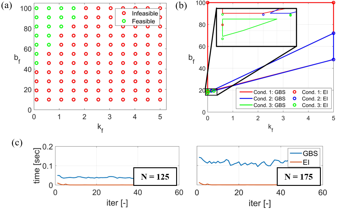
Figure 3: (a) Example of grid-based search of stable region of force-controller gains ($N=20$), (b) Computed results of region of stable force-controller gains by the grid-based search (GBS) and the method using explicit inequalities (EI) and (c) Comparison of computation time for searching stable regions of the force-controller gains when $N=125$ and $N=175$.

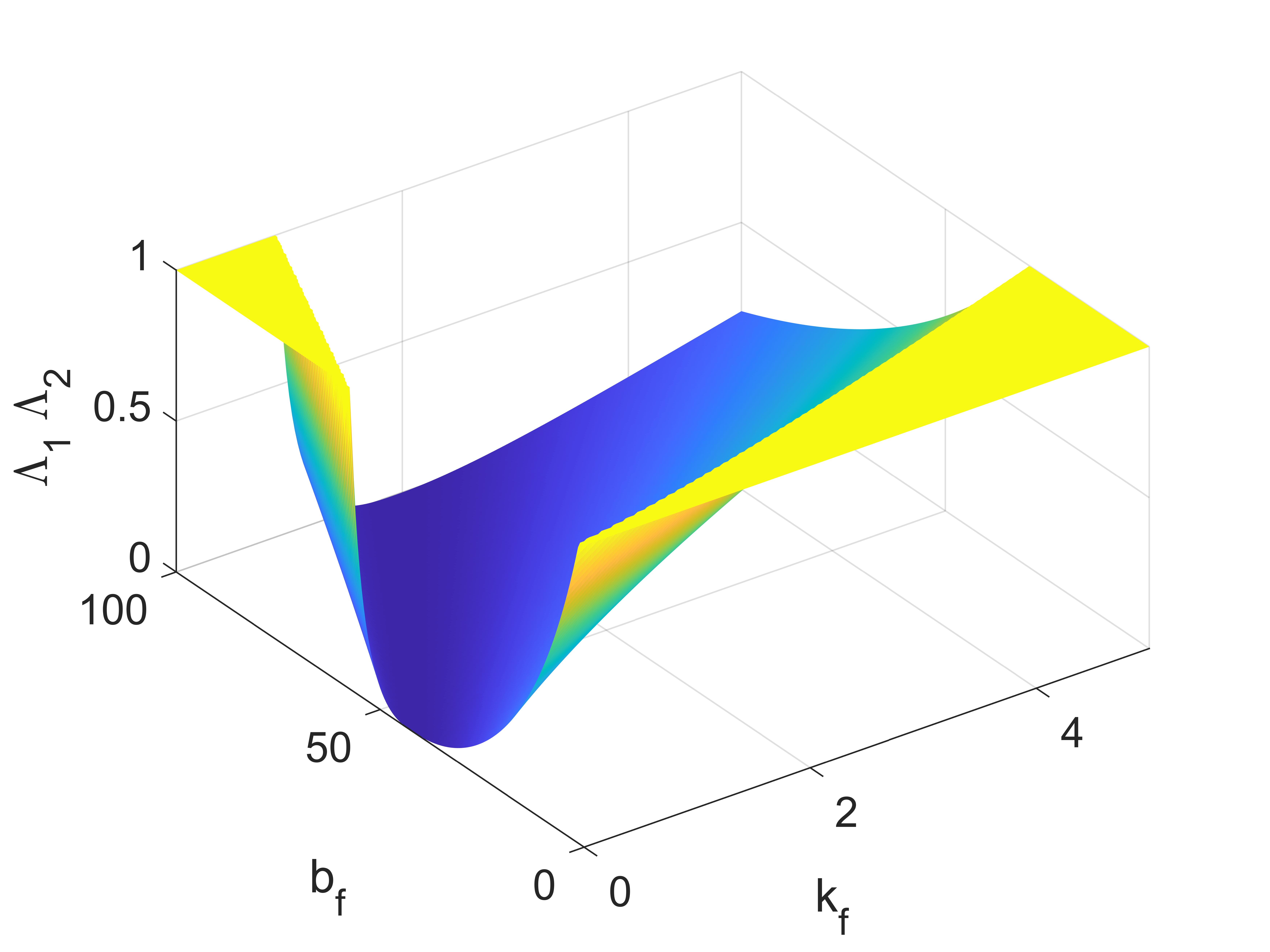
Figure 4: 3D surface map of $\Lambda_{1}\Lambda_{2}$

IV-B1 No-switching condition 1)

If the inequality $4m_{t}k_{p}\leq k_{d}^{2}$ holds, the other conditions are rearranged as follows:

$$\begin{split}-b_{e}(k_{f}+1)+k_{d}<b_{f}\\ \Big{(}\tfrac{k_{e}}{C}-b_{e}\Big{)}k_{f}+\tfrac{k_{e}-k_{p}}{C}+k_{d}-b_{e}<b_{f}\end{split}$$ (19)

where $C\triangleq\tfrac{2K_{1}}{B_{1}-\sqrt{B_{1}^{2}-4K_{1}}}=\tfrac{2k_{p}}{k_{d}-\sqrt{k^{2}_{d}-4m_{t}k_{p}}}$.

IV-B2 No-switching condition 2)

The first and second inequalities are rearranged as follows:

$$\begin{split}-b_{e}(1+k_{f})+k_{d}<b_{f}\\ -b_{e}(1+k_{f})+2\sqrt{m_{t}k_{e}(1+k_{f})}\leq b_{f}.\end{split}$$ (20)

Meanwhile, the third equation is rearranged as follows:

$$(K_{1}+K_{2})B_{2}-2B_{1}K_{2}<(K_{2}-K_{1})\sqrt{B_{2}^{2}-4K_{2}}.$$ (21)

To arrange this inequality in an explicit form, we first need to determine the sign of the left side of (21). If the left side is negative, the above inequality holds, otherwise, we obtain additional conditions by squaring the both sides. After a few computations, the additional condition is arranged as follows:

$$C_{u}k_{p}+(C_{l}k_{e}-b_{e})(1+k_{f})<b_{f}\\ <C_{l}k_{p}+(C_{u}k_{e}-b_{e})(1+k_{f})$$ (22)

where

$$\begin{split}C_{l}\triangleq\tfrac{B_{1}-\sqrt{B_{1}^{2}-4K_{1}}}{2K_{1}},\quad C_{u}\triangleq\tfrac{B_{1}+\sqrt{B_{1}^{2}-4K_{1}}}{2K_{1}}\end{split}$$

when $4m_{t}k_{p}\leq k_{d}^{2}$ holds.

IV-B3 No-switching condition 3)

This condition is rearranged in the form of explicit inequalities as follows:

$$-b_{e}(1+k_{f})+2\sqrt{m_{t}k_{e}(1+k_{f})}\leq b_{f}\\ \leq-b_{e}(1+k_{f})+k_{d}.$$ (23)

IV-B4 Finite-switching condition

Fig. 4 shows that $\Lambda_{1}\Lambda_{2}$ has a bowl shape w.r.t. $k_{f}$ and $b_{f}$. Thus, we can find a globally optimal point of $(k_{f},b_{f})$ which minimizes $J(k_{f},b_{f})$ defined in step 3) using convex optimization. However, since we cannot differentiate $\Lambda_{1}\Lambda_{2}$ due to the modular expression, we need to utilize gradient-free algorithms. Since the given system gets more stable when $\Lambda_{1}\Lambda_{2}$ gets smaller and $(k_{f},b_{f})$ gets further from their limits $[k_{f,m},b_{f,m}]$ and $[k_{f,M},b_{f,M}]$, we set $k_{f}$ and $b_{f}$ to the values which minimize the convex cost function $J(k_{f},b_{f})$ defined in (18) by using the pattern search algorithm.

V Experimental Results

This section reports the experimental validation of the proposed motion/force control strategy.

V-A Experimental Setups

The experimental setup for this research consists of four parts: an underactuated coaxial octocopter, a robotic arm, a 1-axis force sensor and a tilted surface. The coaxial octocopter which weighs 3.78kg was assembled with the custom-built frame, eight KDE2314XF-965 motors with corresponding KDEXF-UAS35 electronic speed controllers, and 9-inch APC LPB09045MR propellers, two Turnigy LiPo batteries for power supplement, and Intel NUC for computing. On Intel NUC, Robot Operating System (ROS) is installed in Ubuntu 18.04, and the position controller for the octocopter, servo-angle controller for the robotic arm and the navigation algorithm with Optitrack are executed. The attitude controllers are executed in Pixhawk 4 which is connected to the Intel NUC. The robotic arm is comprised of ROBOTIS dynamixel XH540 and XM430 servo motors. We mount Honeywell FSS2000NSB 1-axis force sensor to the end-effector which is connected to the arduino nano board. The tilted surface is made of medium density fibreboard (MDF) and we attach four Optitrack markers to that surface to measure its rotation matrix $[B_{f}\ B_{m}]$.

The values of the parameters during the experiments are arranged in Table I.

Estimation of Kelvin-Voigt linear model’s parameters
$\mu_{1}$	$\mu_{2}$	$\rho_{M}$	$k_{e,m}$	$b_{e,m}$	$k_{e,M}$	$b_{e,M}$
0.9996	0.9996	5000	50	0.1	500	1
Reference trajectory generation and controller
$\omega_{n}$	$k_{p}$	$k_{d}$	$K_{m,p}$	$K_{m,d}$
10.0	23.5	19.5	23.5$I_{2}$	19.5$I_{2}$
Force-controller-gain scheduler
$k_{f,m}$	$b_{f,m}$	$k_{f,M}$	$b_{f,M}$
0.1	10	1	40

Table I: Parameters used in the experiments.

We assumed that only the orientation of the contact surface is known while its position is not given. Also, for the constant reference force, $f_{f,r}(t)$ was set to $-6$ while it was set to $-3.5+2.5\cos{\tfrac{2\pi t}{5}}$ for the time-varying reference force.

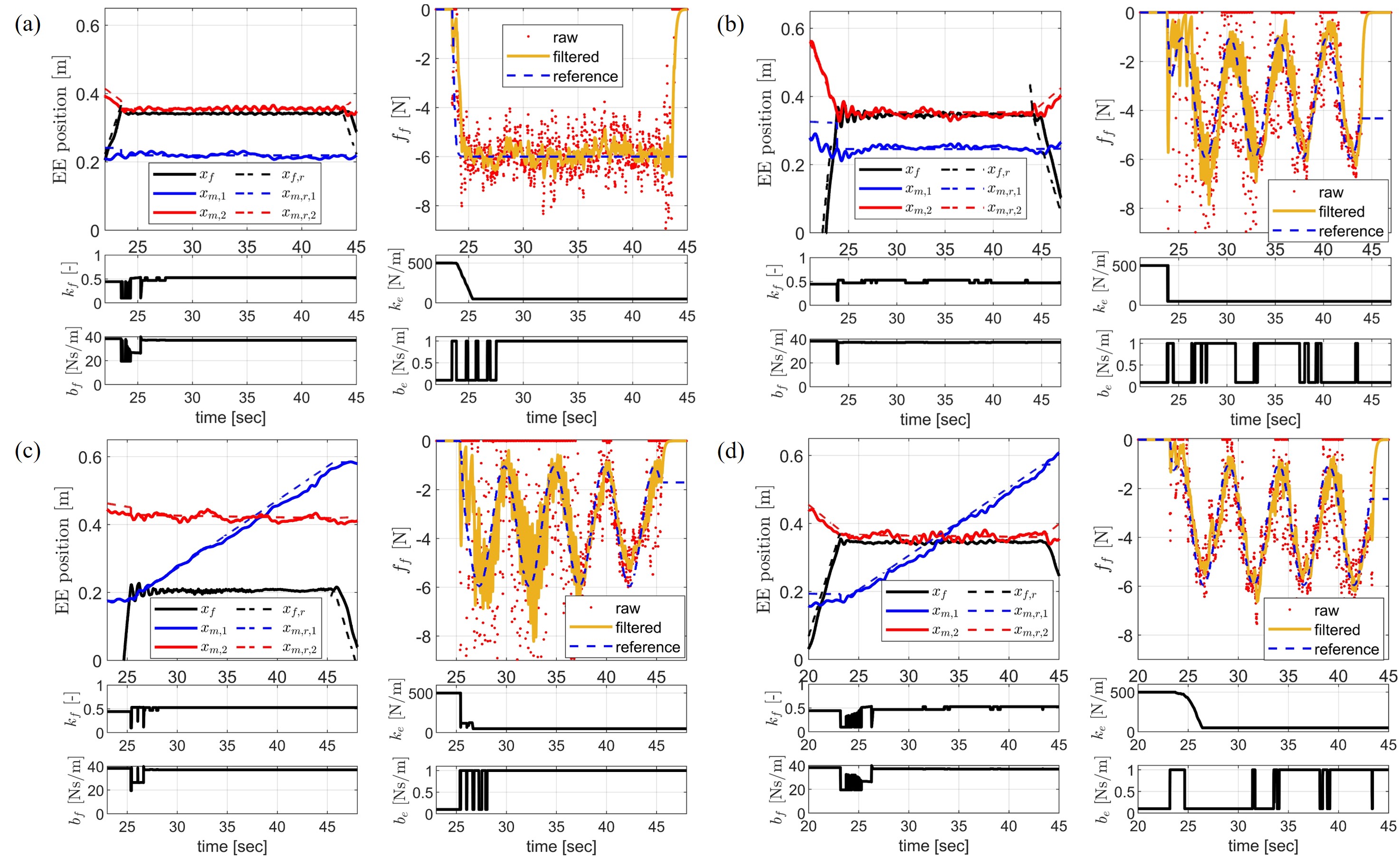
Figure 5: Histories of the end-effector’s position ($p_{e}$), force exerted on the end-effector ($f_{f}$), force-controller gains ($k_{f}$ and $b_{f}$) and estimated environmental parameters ($\hat{k}_{e}$ and $\hat{b}_{e}$) of (a) the first one of Experiment 1, (b) the second one of Experiment 1, (c) the first one of Experiment 2 and (d) the second one of Experiment 2.

V-B Experiment 1: Force Tracking on the Tilted Surface with Two Different Approach Speeds

The uUAM configured with an underactuated coaxial octocopter and a robotic arm approaches the tilted surface with two different approach speeds (0.1 m/s and 0.3 m/s) and exerts the constant or time-varying force onto a specific point of that surface.

Fig. 5a presents the measured values of position and exerted force of the end-effector, the force-controller gains and the estimated environment parameters when the uUAM attempts to exert the constant force to the tilted surface after approaching with the slow speed. As observed in the measured force values, the uUAM was able to track the constant reference force trajectory while keeping the constant position of the end-effector.

In Fig. 5b, contrary to Fig. 5a, the reference force trajectory varied with time and the approach speed was relatively fast. Despite the large oscillations in the force measurement, the stable tracking of the time-varying reference force trajectory was finally attained. From this result, we can notice that the proposed controller can also make the uUAM follow the time-varying reference force after the collision with relatively high speed.

Meanwhile, we can also confirm that the proposed force-controller-gain scheduler successfully generated $k_{f}$ and $b_{f}$ along with the estimated values of $k_{e}$ and $b_{e}$ both in Figs. 5a and 5b.

V-C Experiment 2: Force Tracking while Sliding on the Vertical and Tilted Surfaces

V-C1 Scenario

In this experiment, the uUAM slides on a vertical or tilted surface while exerting the time-varying force for 20 seconds. The approach speed to the vertical surface is set to 0.3 m/s while that to the tilted surface is set to 0.1 m/s.

V-C2 Results

The result of tracking the time-varying reference force trajectory while sliding on the vertical surface is shown in Fig. 5c. The result of $x_{m,1}$ shows that the uUAM successfully slid in the $+y$ direction of the vertical surface while $f_{f}$ followed $f_{f,r}$ after the initial oscillation. This result demonstrates that the proposed controller can make the uUAM simultaneously track the time-varying reference motion and force trajectories even with the high approach speed.

Fig. 5d presents the result of tracking the time-varying force while sliding on the tilted surface. The force tracking performance is enhanced than Fig. 5c due to the lower speed.

VI Conclusions

This paper presents motion/force control that guarantees a stable contact for an aerial manipulator on an arbitrarily tilted surface. To analyze the dynamic characteristics, the translational dynamic equation w.r.t. the position of the end-effector is derived, and decomposed into force and motion spaces where the force exerted on the end-effector is modeled as the Kelvin-Voigt linear model. Then, we estimate the parameters of Kelvin-Voigt linear model by recursive least-squares estimation, and generate the reference motion and force trajectories based on their setpoints. The disturbance-observer-based controller with scheduling of the force-controller gains is designed based on the stability conditions considering both model uncertainty and switching behavior between the free and contact motion. To check the performance of our controller, we conduct four different force tracking experiments with different approach speeds and reference motion/force trajectories. The results confirm that the proposed controller enables the aerial manipulator to simultaneously track the time-varying reference motion and force trajectories while maintaining stable contact. Future works may involve the design of a switching rule which can enhance the stability during the switch between the free and contact motion or a motion/force control law to push a movable structure.

References

- [1] Y. Sun, Z. Jing, P. Dong, J. Huang, W. Chen, and H. Leung, “A switchable unmanned aerial manipulator system for window-cleaning robot installation,” IEEE Robotics and Automation Letters, vol. 6, no. 2, pp. 3483–3490, 2021.
- [2] M. Orsag, C. M. Korpela, S. Bogdan, and P. Y. Oh, “Hybrid adaptive control for aerial manipulation,” Journal of intelligent & robotic systems, vol. 73, no. 1, pp. 693–707, 2014.
- [3] M. Á. Trujillo, J. R. Martínez-de Dios, C. Martín, A. Viguria, and A. Ollero, “Novel aerial manipulator for accurate and robust industrial ndt contact inspection: A new tool for the oil and gas inspection industry,” Sensors, vol. 19, no. 6, p. 1305, 2019.
- [4] M. Allenspach, N. Lawrance, M. Tognon, and R. Siegwart, “Towards 6dof bilateral teleoperation of an omnidirectional aerial vehicle for aerial physical interaction,” arXiv preprint arXiv:2203.03177, 2022.
- [5] E. Shahriari, S. A. B. Birjandi, and S. Haddadin, “Passivity-based adaptive force-impedance control for modular multi-manual object manipulation,” IEEE Robotics and Automation Letters, vol. 7, no. 2, pp. 2194–2201, 2022.
- [6] J. Byun, D. Lee, H. Seo, I. Jang, J. Choi, and H. J. Kim, “Stability and robustness analysis of plug-pulling using an aerial manipulator,” in 2021 IEEE/RSJ International Conference on Intelligent Robots and Systems (IROS). IEEE, 2021, pp. 4199–4206.
- [7] G. Nava, Q. Sablé, M. Tognon, D. Pucci, and A. Franchi, “Direct force feedback control and online multi-task optimization for aerial manipulators,” IEEE Robotics and Automation Letters, vol. 5, no. 2, pp. 331–338, 2019.
- [8] K. Bodie, M. Brunner, M. Pantic, S. Walser, P. Pfändler, U. Angst, R. Siegwart, and J. Nieto, “Active interaction force control for contact-based inspection with a fully actuated aerial vehicle,” IEEE Transactions on Robotics, vol. 37, no. 3, pp. 709–722, 2020.
- [9] L. Peric, M. Brunner, K. Bodie, M. Tognon, and R. Siegwart, “Direct force and pose nmpc with multiple interaction modes for aerial push-and-slide operations,” in 2021 IEEE International Conference on Robotics and Automation (ICRA). IEEE, 2021, pp. 131–137.
- [10] M. Car, A. Ivanovic, M. Orsag, and S. Bogdan, “Impedance based force control for aerial robot peg-in-hole insertion tasks,” in 2018 IEEE/RSJ International Conference on Intelligent Robots and Systems (IROS). IEEE, 2018, pp. 6734–6739.
- [11] L. Marković, M. Car, M. Orsag, and S. Bogdan, “Adaptive stiffness estimation impedance control for achieving sustained contact in aerial manipulation,” in 2021 IEEE international conference on robotics and automation (ICRA). IEEE, 2021, pp. 117–123.
- [12] M. Xu, A. Hu, and H. Wang, “Image-based visual impedance force control for contact aerial manipulation,” IEEE Transactions on Automation Science and Engineering, 2022.
- [13] T. Ikeda, S. Yasui, S. Minamiyama, K. Ohara, S. Ashizawa, A. Ichikawa, A. Okino, T. Oomichi, and T. Fukuda, “Stable impact and contact force control by uav for inspection of floor slab of bridge,” Advanced Robotics, vol. 32, no. 19, pp. 1061–1076, 2018.
- [14] D. Tzoumanikas, F. Graule, Q. Yan, D. Shah, M. Popovic, and S. Leutenegger, “Aerial manipulation using hybrid force and position nmpc applied to aerial writing,” arXiv preprint arXiv:2006.02116, 2020.
- [15] H. W. Wopereis, J. J. Hoekstra, T. H. Post, G. A. Folkertsma, S. Stramigioli, and M. Fumagalli, “Application of substantial and sustained force to vertical surfaces using a quadrotor,” in 2017 IEEE international conference on robotics and automation (ICRA). IEEE, 2017, pp. 2704–2709.
- [16] C. Izaguirre-Espinosa, A.-J. Muñoz-Vázquez, A. Sanchez-Orta, V. Parra-Vega, and P. Castillo, “Contact force tracking of quadrotors based on robust attitude control,” Control Engineering Practice, vol. 78, pp. 89–96, 2018.
- [17] K. Yi, J. Han, X. Liang, and Y. He, “Contact transition control with acceleration feedback enhancement for a quadrotor,” ISA transactions, vol. 109, pp. 288–294, 2021.
- [18] H. Yang and D. Lee, “Dynamics and control of quadrotor with robotic manipulator,” in 2014 IEEE international conference on robotics and automation (ICRA). IEEE, 2014, pp. 5544–5549.
- [19] S. J. Lee, S. H. Kim, and H. J. Kim, “Robust translational force control of multi-rotor uav for precise acceleration tracking,” IEEE Transactions on Automation Science and Engineering, vol. 17, no. 2, pp. 562–573, 2019.
- [20] J. Byun, H. J. Kim, and M. Kwon, “Hybrid motion/force control of the aerial manipulator without information on the added equipment,” in Control Conference (ASCC), 2022 13th Asian. IEEE, 2022.
- [21] Y. Lin, Z. Chen, and B. Yao, “Unified motion/force/impedance control for manipulators in unknown contact environments based on robust model-reaching approach,” IEEE/ASME Transactions on Mechatronics, vol. 26, no. 4, pp. 1905–1913, 2021.
- [22] D. Heck, A. Saccon, N. Van de Wouw, and H. Nijmeijer, “Guaranteeing stable tracking of hybrid position–force trajectories for a robot manipulator interacting with a stiff environment,” Automatica, vol. 63, pp. 235–247, 2016.
- [23] A. Mohammadi, M. Tavakoli, H. J. Marquez, and F. Hashemzadeh, “Nonlinear disturbance observer design for robotic manipulators,” Control Engineering Practice, vol. 21, no. 3, pp. 253–267, 2013.
- [24] C. Audet and J. E. Dennis Jr, “Analysis of generalized pattern searches,” SIAM Journal on optimization, vol. 13, no. 3, pp. 889–903, 2002.