Geodesic slice sampling on the sphere

Abstract

Probability measures on the sphere form an important class of statistical models and are used, for example, in modeling directional data or shapes. Due to their widespread use, but also as an algorithmic building block, efficient sampling of distributions on the sphere is highly desirable. We propose a shrinkage based and an idealized geodesic slice sampling Markov chain, designed to generate approximate samples from distributions on the sphere. In particular, the shrinkage based algorithm works in any dimension, is straight-forward to implement and has no tuning parameters. We verify reversibility and show that under weak regularity conditions geodesic slice sampling is uniformly ergodic. Numerical experiments show that the proposed slice samplers achieve excellent mixing on challenging targets including the Bingham distribution and mixtures of von Mises-Fisher distributions. In these settings our approach outperforms standard samplers such as random-walk Metropolis Hastings and Hamiltonian Monte Carlo.

1 Introduction

In recent years, with the advent of sampling methods based on Markov chains, Bayesian inference with posterior distributions on manifolds attracted considerable attention. In particular, various Markov chain based algorithms for approximate sampling of posterior distributions on manifolds have been developed, see for example [BG13, LZS14, GS19, LRSS22, BK22]. Here we focus on the prototypical case of the sphere embedded in $\mathbb{R}^{d}$ as the underlying manifold. Following the slice sampling paradigm, we introduce and analyse an efficient way for approximate sampling of distributions on the sphere.

Let $\mathbb{S}^{d-1}$ be the $(d-1)$-dimensional Euclidean unit sphere in $\mathbb{R}^{d}$ and let $\sigma_{d-1}$ denote the volume measure on $\mathbb{S}^{d-1}$. For $p\colon\mathbb{S}^{d-1}\to(0,\infty)$ satisfying

$$Z\coloneqq\int_{\mathbb{S}^{d-1}}p(x)\sigma_{d-1}({\rm d}x)\in(0,\infty),$$ (1)

we are interested in a target distribution $\pi$ of the form

$$\pi({\rm d}x)=\frac{1}{Z}\,p(x)\sigma_{d-1}({\rm d}x)$$ (2)

such that $p/Z$ is the probability density function of $\pi$ relative to $\sigma_{d-1}$. In a Bayesian setting, $\pi$ can be considered a posterior distribution determined by likelihood $p$ and prior measure $\sigma_{d-1}$. Throughout the paper, we assume that $p$ can be evaluated, which is a common minimal requirement in the Markov chain Monte Carlo (MCMC) literature.

Our motivation for considering MCMC on the sphere is twofold:

1. Posteriors naturally defined on the sphere require efficient sampling: Sampling distributions on the sphere play an important role in directional statistics and shape analysis, see [MJ00], and Bayesian inverse problems on $\mathbb{S}^{2}$ occur, e.g., in astrophysics or geophysics (see [MMFK22] for a list of some examples). Moreover, Bayesian density estimation [HLSS20] requires sampling of a posterior on an infinite-dimensional sphere, which usually is approximated by truncating the dimension, ending up with $\mathbb{S}^{d-1}$ for large $d$

2. Spherical sampling can be used as tool within transforming Markov chains: Lan et al. introduced a Hamiltonian Monte Carlo (HMC) scheme for sampling from spherical distributions to efficiently sample from distributions in $\mathbb{R}^{d}$ constrained by inequalities [LZS14]. Recently, Yang et al. demonstrated that MCMC algorithms on $\mathbb{S}^{d-1}$ can target distributions in $\mathbb{R}^{d}$ by mapping them to the sphere by means of the stereographic projection [YŁR22]. They report that for their proposed algorithms this approach is advantageous in heavy-tailed distribution scenarios.

We follow the slice sampling paradigm for approximately simulating $\pi$, since it allows us to avoid local random walk behavior, no tuning of a parameter such as a step-size is required and usually a richer choice of possible updates is offered, for details see [Nea03, MAM10]. A transition mechanism for realizing a corresponding Markov chain works as follows: Given current state $x\in\mathbb{S}^{d-1}$, a superlevel set $L(t)$ of $p$ is randomly determined by choosing a level $t\in(0,p(x))$. Then, the next Markov chain instance is specified by (mimicking) sampling of the normalized reference measure $\sigma_{d-1}$ restricted to the levelset. The latter step requires some care regarding its algorithmic design. We propose to randomly choose a great circle on the sphere that forms a geodesic through the current state. Then, ideally, we draw by acceptance/rejection uniformly distributed in the levelset intersected with the geodesic. Alternatively, we use a shrinkage procedure, proposed in [Nea03], to draw the next instance from the intersection. We refer to the first version of the sampling algorithm as the ideal and the second version as the shrinkage-based geodesic slice sampler.

The main contributions of our paper are:

• We introduce an ideal geodesic slice sampler with corresponding Markov kernel $H$ for approximately simulating $\pi$. The kernel $H$ moves along great circles on $\mathbb{S}^{d-1}$ and can be algorithmically realized by using an univariate acceptance/rejection approach.

• To efficiently simulate the uniform distribution on the intersection of the superlevel set with a great circle containing the current state, we modify the ideal transition mechanism by using the shrinkage procedure introduced in [Nea03] and obtain a corresponding Markov kernel $\widetilde{H}$. This strategy is also used in the elliptical slice sampling approach [MAM10].

• We show reversibility with respect to the target distribution $\pi$ for both $H$ and $\widetilde{H}$. This leads to the well-definedness of both algorithms.

• We prove uniform ergodicity with explicit constants for target densities $p$ that satisfy a boundedness condition. We provide total variation distance estimates of the $n$th marginal of a Markov chain with transition kernel $H$ or $\widetilde{H}$ to $\pi$, see Theorem 15 and Theorem 26.

• We test our algorithms on challenging targets such as the Bingham distribution and mixtures of von Mises-Fisher distributions. We observe that our slice samplers outperform standard samplers such as random walk Metropolis Hastings (RWMH) and Hamiltonian Monte Carlo (HMC) on spherical distributions.

Let us comment on how our contributions fit into the literature. In [LRSS22] Lie et al. present two MCMC algorithms to sample distributions on the sphere utilizing push forward kernels of a preconditioned Crank-Nicolson algorithm and of elliptical slice sampling, respectively. The crucial difference to our work is that Lie et al. assume that the target density is defined relative to an angular Gaussian distribution. Instead, here we consider target densities relative to the volume measure of the sphere. Observe that with increasing dimension both reference measures become ‘increasingly singular’ to each other. Furthermore, Marignier et al. propose in [MMFK22] a proximal MCMC method to sample from posterior distributions of inverse imaging problems on $\mathbb{S}^{2}$. An infinite-dimensional setting of Bayesian density estimation is treated in [HLSS20] by an HMC algorithm on a sphere. Other MCMC approaches have been developed on more general manifolds that usually cover $\mathbb{S}^{d-1}$ as a special case. This includes the HMC algorithm for manifolds embedded in Euclidean space introduced in [BG13] which utilizes the geodesic flow. Furthermore, in [GS19] a Metropolis-Hastings-like geodesic walk on manifolds with non-negative curvature is investigated. There are some similarities between their geodesic walk and our algorithms: A geodesic is sampled and then moves on the geodesic are proposed as next step. However, in [GS19] the move on the geodesic is performed by a Metropolis-Hastings-like acceptance/rejection step, whereas we rely on slice sampling incorporating the geodesic. Here it is also worth to mention that several geodesic walks exist that target the uniform distribution on subsets of the sphere. We refer to Section 2.5 for more details. Finally, note that recently there has been some theoretical progress in the investigation of convergence properties of slice sampling, see for example [ŁR14, NRS21b, NRS21a, HNR23] that very much influenced the presentation and proof arguments of our theoretical results.

The outline of our paper is as follows: We start by introducing the setting, notation and the results for manifolds that are required to argue for the algorithmic design and well-definedness. In Section 3, we formulate the ideal and shrinkage slice sampler in terms of the transition kernel and transition mechanism. Here we also prove the reversibility and uniform ergodicity statements. Next we illustrate the applicability of our approach in different scenarios using numerical experiments. We conclude with a discussion of our findings.

2 Preliminaries

In this section we provide some general notation and introduce several objects on the sphere relevant to us.

2.1. Setting and Notation.

For $d\in\mathbb{N}$ let $\lambda_{d}$ be the Lebesgue measure on $\mathbb{R}^{d}$, and let $\left\|\cdot\right\|$ be the Euclidean norm induced by the standard inner product ${x}^{T}\!{y}$, where $x,y\in\mathbb{R}^{d}$. Throughout this paper we assume $d\geq 3$. We consider the $(d-1)$-dimensional Euclidean unit sphere

$$\mathbb{S}^{d-1}\coloneqq\{x\in\mathbb{R}^{d}\mid\left\|x\right\|=1\},\qquad d\in\mathbb{N},$$

equipped with the Borel-$\sigma$-algebra $\mathcal{B}\left(\mathbb{S}^{d-1}\right)$ and the canonical volume measure $\sigma_{d-1}$. We denote the volume of the $(d-1)$-dimensional sphere by $\omega_{d-1}\coloneqq\sigma_{d-1}\left(\mathbb{S}^{d-1}\right)$. Moreover, we let $\mathrm{Id}_{d}\in\mathbb{R}^{d\times d}$ be the $d$-dimensional identity matrix and note that the essential supremum norm of $p\colon\mathbb{S}^{d-1}\to(0,\infty)$ is given by

$$\left\|p\right\|_{\infty}:=\operatornamewithlimits{ess\,sup}_{x\in\mathbb{S}^{d-1}}p(x)=\inf_{\begin{subarray}{c}N\in\mathcal{B}\left(\mathbb{S}^{d-1}\right),\\ \sigma_{d-1}(N)=0\end{subarray}}\quad\sup_{x\in\mathbb{S}^{d-1}\setminus N}p(x).$$

We stress that $\left\|p\right\|_{\infty}$ may take values in $\mathbb{R}_{+}\cup\{\infty\}$.

Remark 1.

We consider strictly positive $p$, but can also treat unnormalized density functions that are $[0,\infty)$-valued using the following modification: In case $p$ reaches zero, we restrict the state space of our slice sampling algorithms to the set

$$\{x\in\mathbb{S}^{d-1}\mid p(x)>0\}.$$

All arguments can then be performed analogously.

We introduce some useful notation. For a topological space $\mathcal{X}$ let $\mathcal{B}\left(\mathcal{X}\right)$ be the corresponding Borel-$\sigma$-algebra on $\mathcal{X}$. We denote the restriction of any measure $\nu$ on $(\mathcal{X},\mathcal{B}\left(\mathcal{X}\right))$ to a set $A\in\mathcal{B}\left(\mathcal{X}\right)$ by $\nu|_{A}$, that is $\nu|_{A}(B)=\nu(A\cap B)$ for all $B\in\mathcal{B}\left(\mathcal{X}\right)$. Additionally, the Dirac measure at $z\in\mathcal{X}$ is written as $\delta_{z}$. Moreover, we denote the uniform distribution $\frac{1}{\lambda_{1}(A)}\,\lambda_{1}|_{A}$ on $A\in\mathcal{B}\left(\mathbb{R}\right)$ as $\mathcal{U}(A)$.

Assume that $\nu$ and $\mu$ are two probability measures on $(\mathcal{X},\mathcal{B}\left(\mathcal{X}\right))$. Then

$$d_{tv}\left(\mu,\nu\right)\coloneqq\sup_{A\in\mathcal{B}\left(\mathcal{X}\right)}|\mu(A)-\nu(A)|$$

denotes the total variation distance between $\mu$ and $\nu$.

We say that a Markov kernel $P$ on $\mathcal{X}\times\mathcal{B}\left(\mathcal{X}\right)$ is uniformly ergodic if there exist constants $\kappa<\infty$ and $\rho\in(0,1)$ such that

$$\sup_{x\in\mathcal{X}}d_{tv}\left(P^{n}(x,\cdot),\eta\right)\leq\kappa\rho^{n},\qquad\forall\,n\in\mathbb{N},$$

where $\eta$ is the stationary probability measure of $P$.

Sometimes it is more convenient to work with random variables. Therefore, let $(\Omega,\mathcal{F},\mathbb{P})$ be a sufficiently rich probability space on which all random variables occurring in this paper are defined. If a random variable $X$ has distribution $\nu$, we write $X\sim\nu$.

2.2. Geodesics on the Sphere.

For a given point $x\in\mathbb{S}^{d-1}$ we call

$${\mathbb{S}^{d-2}_{x}}\coloneqq\{v\in\mathbb{S}^{d-1}\mid{v}^{T}\!{x}=0\}$$

the great subsphere with pole $x$. Then every pair $(x,v)$ where $x\in\mathbb{S}^{d-1}$ and $v\in{\mathbb{S}^{d-2}_{x}}$ determines a great circle on $\mathbb{S}^{d-1}$, namely

$$\gamma_{(x,v)}:\mathbb{R}\to\mathbb{S}^{d-1},\qquad\theta\mapsto\cos(\theta)x+\sin(\theta)v.$$

Note that $\gamma_{(x,v)}$ is $2\pi$-periodic due to the periodicity of sine and cosine.

Since $\mathbb{S}^{d-1}$ is a complete Riemannian manifold, we want to relate the objects we just defined to tangent spaces, geodesics and unit tangent spheres defined on general Riemannian manifolds. This will enable us to apply results on the geodesic flow. For an introduction to Riemannian manifolds see e.g. [Boo86].

Let $x\in\mathbb{S}^{d-1}$. Then the tangent space to $\mathbb{S}^{d-1}$ at $x$ is

$$E_{x}\coloneqq\{y\in\mathbb{R}^{d}\mid{y}^{T}\!{x}=0\},$$

see e.g. [RS22, Example 2.2.6], equipped with the standard Euclidean metric. Therefore, ${\mathbb{S}^{d-2}_{x}}$ is the unit sphere in the tangent space to $\mathbb{S}^{d-1}$ at $x$. Moreover, the geodesics on the sphere coincide with the great circles. Since $\mathbb{S}^{d-1}$ is compact, for each $x\in\mathbb{S}^{d-1}$ and all $v$ in the tangent unit sphere at $x$, i.e. $v\in{\mathbb{S}^{d-2}_{x}}$, there exists as unique geodesic $\gamma:\mathbb{R}\to\mathbb{S}^{d-1}$ with $\gamma(0)=x$ and velocity vector $v$. This geodesic is exactly $\gamma_{(x,v)}$, see also [Pet16, Section 5.2].

We denote the natural volume measure on ${\mathbb{S}^{d-2}_{x}}$ as $\mu_{x}$. Let $e_{1}^{(x)},\ldots,e_{d-1}^{(x)}\in E_{x}$ be an orthonormal basis of $E_{x}$. Then

$$\varphi_{x}:\mathbb{R}^{d-1}\to E_{x},\qquad(y_{1},\ldots,y_{d-1})\mapsto\sum_{i=1}^{d-1}y_{i}e_{i}^{(x)}$$ (3)

is an isometry and thus $\varphi_{x}(\mathbb{S}^{d-2})={\mathbb{S}^{d-2}_{x}}$. Since isometries preserve volume, we have $\mu_{x}=\varphi_{x}(\sigma_{d-2})$ for all $x\in\mathbb{S}^{d-1}$, that is,

$$\mu_{x}(A)=\sigma_{d-2}\left(\varphi_{x}^{-1}(A)\right),\qquad\forall\,A\in\mathcal{B}\left({\mathbb{S}^{d-2}_{x}}\right),$$ (4)

see also [Mun91, Exercise 25.4]. In particular, this implies $\mu_{x}({\mathbb{S}^{d-2}_{x}})=\omega_{d-2}$.

2.3. Level Sets.

We denote the superlevel set for level $t\in\mathbb{R}_{+}$ as

$$L(t):=\{x\in\mathbb{S}^{d-1}\mid p(x)>t\}.$$

In the following we also make use of geodesic level sets, i.e., intersections of superlevel sets and geodesics

$$L(x,v,t):=\{\theta\in[0,2\pi)\mid p\left(\gamma_{(x,v)}(\theta)\right)>t\}$$

for $x\in\mathbb{S}^{d-1}$, $v\in{\mathbb{S}^{d-2}_{x}}$ and $t\in\mathbb{R}_{+}$.

We observe that

$$\mathbbm{1}_{L(t)}\big{(}\gamma_{(x,v)}(\theta)\big{)}=\mathbbm{1}_{L(x,v,t)}(\theta).$$ (5)

Our integrability assumption on $p$ ensures that geodesic level sets are not ‘too small’. This is formalized in the following lemma, which is proved in Section A.4.

Lemma 2.

For $x\in\mathbb{S}^{d-1}$ and $t\in(0,\left\|p\right\|_{\infty})$ define

$$V(x,t)\coloneqq\{v\in{\mathbb{S}^{d-2}_{x}}\mid\lambda_{1}\big{(}L(x,v,t)\big{)}>0\}.$$

Then for $\frac{1}{\omega_{d-1}}\,\sigma_{d-1}$- almost all $x\in\mathbb{S}^{d-1}$ we have

$$\frac{1}{p(x)}\lambda_{1}\left(\left\{t\in(0,p(x))\,\biggl{|}\,\,\frac{1}{\omega_{d-2}}\biggr{.}\,\mu_{x}(V(x,t))=1\right\}\right)=1.$$

2.4. Liouville Measure.

We now introduce a measure on

$$\mathcal{S}\mathbb{S}^{d-1}\coloneqq\bigcup_{x\in\mathbb{S}^{d-1}}\big{(}\{x\}\times{\mathbb{S}^{d-2}_{x}}\big{)},$$

the so called Liouville measure defined by

$$\mathcal{L}(A):=\int_{\mathbb{S}^{d-1}}\int_{{\mathbb{S}^{d-2}_{x}}}\mathbbm{1}_{A}(x,v)\mu_{x}({\rm d}v)\sigma_{d-1}({\rm d}x),\qquad A\in\mathcal{B}\left(\mathcal{S}\mathbb{S}^{d-1}\right).$$ (6)

Moreover, we define the map

$$T_{\theta}:\mathcal{S}\mathbb{S}^{d-1} \to\mathcal{S}\mathbb{S}^{d-1}$$

$$(x,v) \mapsto\big{(}\cos(\theta)x+\sin(\theta)v,\sin(\theta)x-\cos(\theta)v\big{)}$$

for $\theta\in\mathbb{R}$. The following observation is central to our proof techniques.

Lemma 3.

Let $F:\mathcal{S}\mathbb{S}^{d-1}\to\mathbb{R}$ be a function that is integrable with respect to the Liouville measure $\mathcal{L}$. Then

$$\int_{\mathcal{S}\mathbb{S}^{d-1}}F(y)\mathcal{L}({\rm d}y)=\int_{\mathcal{S}\mathbb{S}^{d-1}}F\left(T_{\theta}(y)\right)\mathcal{L}({\rm d}y)$$ (7)

holds for all $\theta\in\mathbb{R}$.

This invariance of the Liouville measure under the map $T_{\theta}$ results from the invariance of $\mathcal{L}$ under the geodesic flow and the invariance of $\mu_{x}$ under flipping the sign of the second component. Note that identity (7) already appears in the proof of [GS19, Theorem 27] in a setting of more general manifolds. Nonetheless, for the convenience of the reader we provide the details of the proof for Lemma 3 in Appendix A.3.

The behaviour of some of the previously defined objects under the map $T_{\theta}$ for $\theta\in\mathbb{R}$ is summarized in the following lemma, which is proved in Section A.2.

Lemma 4.

Let $x\in\mathbb{S}^{d-1}$, $v\in{\mathbb{S}^{d-2}_{x}}$ and $t\in(0,\left\|p\right\|_{\infty})$. Then we have

1. $\gamma_{(x,v)}(\theta-r)=\gamma_{T_{\theta}(x,v)}(r)$ for all $r\in\mathbb{R}$,

2. $\gamma_{T_{\theta}(x,v)}(\theta)=x$,

3. $\lambda_{1}\big{(}L(T_{\theta}(x,v),t)\big{)}=\lambda_{1}\big{(}L(x,v,t)\big{)}$,

for all $\theta\in\mathbb{R}$.

2.5. Geodesic Walk on the Sphere.

We describe our principal approach for generating a next point on the sphere given a current position $x\in\mathbb{S}^{d-1}$ by following geodesics. The transition to the next point comprises two steps:

1. Choose a random geodesic $\gamma$ through the given point $x$.

2. Choose a random point on the geodesic $\gamma$.

Remark 5.

The appeal of this approach is twofold. First, the geodesics on the $(d-1)$-dimensional sphere are available in an explicit form that is easy to evaluate thereby allowing for cheap exact computations. Second, sampling from a geodesic is a one-dimensional problem. Here, it can even be reduced to a problem on an interval of length $2\pi$ due to the periodicity of the geodesics on $\mathbb{S}^{d-1}$.

The first step in the outlined approach relies on the fact that the geodesics through $x\in\mathbb{S}^{d-1}$ are parametrized by ${\mathbb{S}^{d-2}_{x}}$. Therefore, choosing a random geodesic boils down to sampling a point $v$ from the uniform distribution $\frac{1}{\omega_{d-2}}\,\mu_{x}$ on ${\mathbb{S}^{d-2}_{x}}$. This uniquely determines the geodesic $\gamma_{(x,v)}$. Section A.1 presents a simple algorithm to sample from $\frac{1}{\omega_{d-2}}\,\mu_{x}$.

The mechanism of the second step crucially influences the stationary distribution of the resulting Markov chain. We will first discuss the use of a fixed probability distribution in this step, which causes the stationary distribution to be uniform. In Section 3, we explain how the second step can be modified so as to obtain a Markov chain with prespecified stationary distribution that can be almost arbitrary.

Let $\tau$ be a probability distribution on $[0,2\pi)$. Using this distribution to sample from the geodesic, we obtain the following Markov kernel

$$K_{\tau}(x,A)\coloneqq\frac{1}{\omega_{d-2}}\int_{{\mathbb{S}^{d-2}_{x}}}\int_{[0,2\pi)}\mathbbm{1}_{A}\left(\gamma_{(x,v)}(\theta)\right)\tau({\rm d}\theta)\mu_{x}({\rm d}v),$$

with $x\in\mathbb{S}^{d-1},A\in\mathcal{B}\left(\mathbb{S}^{d-1}\right)$. The corresponding transition mechanism is described in Algorithm 1. Observe that $\tau$ can be interpreted as the distribution of the step-size of the algorithm.

Algorithm 1 Geodesic random walk on the sphere.

input: current state $x\in\mathbb{S}^{d-1}$
output: next state $x^{\prime}$

1:  Draw $V\sim\frac{1}{\omega_{d-2}}\,\mu_{x}$, call the result $v$.

2:  Draw $\Theta\sim\tau$, call the result $\theta$.

3:  Set $x^{\prime}=\cos(\theta)x+\sin(\theta)v$.

Lemma 3 implies reversibility of $K_{\tau}$ with respect to the uniform distribution $\sigma_{d-1}$. More precisely, let $A,B\in\mathcal{B}\left(\mathbb{S}^{d-1}\right)$ and set

$$F_{\theta}(x,v)\coloneqq\mathbbm{1}_{B}(x)\mathbbm{1}_{A}\big{(}\gamma_{(x,v)}(\theta)\big{)},\qquad x\in\mathbb{S}^{d-1},v\in{\mathbb{S}^{d-2}_{x}},\theta\in[0,2\pi).$$

Then Lemma 3 and Lemma 4.ii yield

$$\omega_{d-2}\int_{B}K_{\tau}(x,A)\ \sigma_{d-1}({\rm d}x)$$

$$\qquad=\int_{\mathbb{S}^{d-1}}\int_{{\mathbb{S}^{d-2}_{x}}}\int_{[0,2\pi)}\mathbbm{1}_{B}(x)\mathbbm{1}_{A}\left(\gamma_{(x,v)}(\theta)\right)\tau({\rm d}\theta)\,\mu_{x}({\rm d}v)\,\sigma_{d-1}({\rm d}x)$$

$$\qquad=\int_{[0,2\pi)}\int_{\mathcal{S}\mathbb{S}^{d-1}}F_{\theta}(x,v)\ \mathcal{L}({\rm d}(x,v))\,\tau({\rm d}\theta)$$

$$\qquad=\int_{[0,2\pi)}\int_{\mathcal{S}\mathbb{S}^{d-1}}(F_{\theta}\circ T_{\theta})(x,v)\ \mathcal{L}({\rm d}(x,v))\,\tau({\rm d}\theta)$$

$$\qquad=\int_{\mathbb{S}^{d-1}}\int_{{\mathbb{S}^{d-2}_{x}}}\int_{[0,2\pi)}\mathbbm{1}_{B}\left(\gamma_{(x,v)}(\theta)\right)\mathbbm{1}_{A}(x)\ \tau({\rm d}\theta)\,\mu_{x}({\rm d}v)\,\sigma_{d-1}({\rm d}x)$$

$$\qquad=\omega_{d-2}\int_{A}K_{\tau}(x,B)\ \sigma_{d-1}({\rm d}x).$$

Remark 6.

Applying results of either [LV18] or [GS19, Theorem 27] to $\mathbb{S}^{d-1}$ also yields reversibility of $K_{\tau}$ with respect to the uniform distribution $\sigma_{d-1}$.

Note that, depending on how $\tau$ is chosen, $K_{\tau}$ coincides with different random walks that have been discussed in the literature. We add some remarks on that:

Remark 7 (Refers to [MS18]).

If we choose the step-size to be constant, that is, $\tau=\delta_{\varepsilon}$ for a fixed $\varepsilon\in[0,2\pi)$, then we obtain the geodesic walk from [MS18] for the special case of the sphere. In [MS18], Mangoubi and Smith provide dimension independent mixing time results for this walk on manifolds with bounded positive sectional curvature.

Remark 8 (Refers to [GS19]).

For targeting the uniform distribution on the sphere, the geodesic random walk introduced in [GS19, Algorithm 1, choose $K=\mathbb{S}^{d-1}$] corresponds to $K_{\tau}$ with $\tau$ being the distribution of $\varepsilon R$, where $R$ is a chi-distributed random variable with $d-1$ degrees of freedom and fixed $\varepsilon>0$. For manifolds with non-negative sectional curvature and bounded Riemannian curvature tensor, Goyal and Shetty provide mixing time results if their unfiltered walk is modified to target the uniform distribution of a strongly convex subset of the ambient manifold.

Remark 9 (Refers to [HSSW22]).

The kernel $K_{\delta_{\varepsilon}}$ from Remark 7 is related to the retraction-based random walk introduced in [HSSW22], where the geodesics are replaced by retractions, i.e. second order approximations of the geodesics. Herrmann et al. show that for $\varepsilon\to 0$ this algorithm can be used to sample paths of the Brownian motion on a general manifold. Note, however, that this causes the stationary distribution of the resulting Markov chain to deviate from the uniform distribution.

Remark 10 (Refers to Givens rotation).

Transitions according to $K_{\tau}$ can also be interpreted as the repeated action of random rotations. The $d$-dimensional rotation matrix

$$G(y,z,\theta)=\,\,\mathrm{Id}_{d}+(\cos(\theta)-1)(yy^{T}+zz^{T})+\sin(\theta)\,(yz^{T}-zy^{T})$$ (8)

is the Givens rotation acting in the plane spanned by two orthogonal directions $y,z\in\mathbb{S}^{d-1}$ where $\theta$ is the rotation angle, see [Giv58]. In this view, a transition of $K_{\tau}$ to the next state $X^{\prime}$ is achieved by drawing an axis $V\sim\mathcal{U}({\mathbb{S}^{d-2}_{x}})$ and an angle $\Theta\sim\tau$ to form a random Givens rotation that is applied to the current state $x$, i.e.

$$X^{\prime}=G(V,x,\Theta)\,x.$$ (9)

Remark 11 (Refers to Kac’s walk).

Reformulation (9) can be viewed as a generalization of Kac’s random walk on the sphere, see e.g. [Kac56, PS17]. To perform a transition of Kac’s walk, draw $1\leq I<J\leq d$ and $\Theta\sim\mathcal{U}(0,2\pi)$ randomly to generate the next state $X^{\prime}$ by rotating the current state $x$, i.e.

$$X^{\prime}=G(e_{I},e_{J},\Theta)\,x$$ (10)

where $\{e_{i}\}_{i=1}^{d}$ is the standard basis of $\mathbb{R}^{d}$.

Kac’s walk also approximately simulates the uniform distribution, but chooses the plane of rotation from a discrete set, whereas in the generalized version (9), the plane of rotation changes continuously and always contains the current state $x$. In [PS17], Pillai and Smith show optimal mixing time results for Kac’s walk.

3 Geodesic Slice Sampling in $\mathbb{S}^{d-1}$

Our main goal is to construct a Markov chain that can be used for approximate sampling of the probability distribution $\pi$ defined in (2). To do so, we combine a slice sampling strategy with the approach to walk the sphere described in Section 2.5. More precisely, in each iteration we run a one-dimensional slice sampler on a randomly chosen geodesic through the current state.

3.1. Ideal Geodesic Slice Sampling

We start by presenting a rejection sampling based version of the geodesic slice sampler. For $x\in\mathbb{S}^{d-1}$, $t\in(0,p(x))$ and $A\in\mathcal{B}\left(\mathbb{S}^{d-1}\right)$ let

$$H_{t}(x,A)\coloneqq\frac{1}{\omega_{d-2}}\int_{{\mathbb{S}^{d-2}_{x}}}\frac{1}{\lambda_{1}(L(x,v,t))}\int_{L(x,v,t)}\mathbbm{1}_{A}\left(\gamma_{(x,v)}(\theta)\right)\,{\rm d}\theta\,\mu_{x}({\rm d}v).$$

We call the algorithm simulating the Markov kernel

$$H(x,A)\coloneqq\frac{1}{p(x)}\int_{0}^{p(x)}H_{t}(x,A)\,{\rm d}t,\qquad x\in\mathbb{S}^{d-1},A\in\mathcal{B}\left(\mathbb{S}^{d-1}\right),$$ (11)

the ideal geodesic slice sampler. A single transition of it is described in Algorithm 2.

Algorithm 2 Ideal geodesic slice sampler.

input: current state $x\in\mathbb{S}^{d-1}$
output: next state $x^{\prime}$

1:  Draw $V\sim\frac{1}{\omega_{d-2}}\,\mu_{x}$, call the result $v$.

2:  Draw $\Upsilon\sim\mathcal{U}(0,p(x))$, call the result $t$.

3:  repeat

4:   Draw $\Theta\sim\mathcal{U}(0,2\pi)$, call the result $\theta$.

5:   Set $x^{\prime}=\cos(\theta)x+\sin(\theta)v$.

6:  until $p(x^{\prime})>t$.

Note that $H$ is well defined for $\frac{1}{\omega_{d-1}}\,\sigma_{d-1}$-almost all $x\in\mathbb{S}^{d-1}$ due to Lemma 2. On the $\sigma_{d-1}$-null set where (11) is not well defined, we set $H(x,\cdot)=\frac{1}{\omega_{d-1}}\,\sigma_{d-1}$ for the sake of completeness.

Remark 12.

The geodesic slice sampler can be viewed as realisation of the procedure described in Section 2.5 where the second step utilizes a distribution on the geodesic that depends on the initial point $x$ and the chosen geodesic $\gamma$.

A useful tool for showing reversibility of Markov kernels exhibiting the same structure as the ideal geodesic slice sampling kernel is Lemma 1 from [ŁR14]. It applies to subsets of $\mathbb{R}^{d}$ in its original formulation, but can be extended to arbitrary $\sigma$-finite measure spaces. For the convenience of the reader we adapt the relevant parts of the aforementioned lemma to our setting.

Lemma 13.

Let

$$P(x,A)\coloneqq\frac{1}{p(x)}\int_{0}^{p(x)}P_{t}(x,A)\,{\rm d}t,\qquad x\in\mathbb{S}^{d-1},A\in\mathcal{B}\left(\mathbb{S}^{d-1}\right),$$

be a Markov kernel where $P_{t}:\mathbb{S}^{d-1}\times\mathcal{B}\left(\mathbb{S}^{d-1}\right)\to[0,1]$ for $t\in(0,\left\|p\right\|_{\infty})$ are themselves Markov kernels. If $P_{t}$ is reversible with respect to $\frac{1}{\sigma_{d-1}(L(t))}\,\sigma_{d-1}|_{L(t)}$ for all $t\in(0,\left\|p\right\|_{\infty})$, then $P$ is reversible with respect to $\pi$.

Utilizing this lemma we obtain the following reversibility result for $H$.

Lemma 14.

For $\pi$ defined as in (2), the kernel $H$ is reversible with respect to $\pi$.

Proof.

Let $t\in(0,\left\|p\right\|_{\infty})$ and $A,B\in\mathcal{B}\left(\mathbb{S}^{d-1}\right)$. Lemma 3 implies

$$\omega_{d-2}\int_{B\cap L(t)}H_{t}(x,A)\,\sigma_{d-1}({\rm d}x)$$

$$\quad=\int_{B\cap L(t)}\int_{{\mathbb{S}^{d-2}_{x}}}\frac{1}{\lambda_{1}(L(x,v,t))}\int_{L(x,v,t)}\mathbbm{1}_{A}\big{(}\gamma_{(x,v)}(\theta)\big{)}\,{\rm d}\theta\,\mu_{x}({\rm d}v)\,\sigma_{d-1}({\rm d}x)$$

$$\quad=\int_{[0,2\pi)}\int_{\mathbb{S}^{d-1}}\int_{{\mathbb{S}^{d-2}_{x}}}\frac{\mathbbm{1}_{L(T_{\theta}(x,v),t)}(\theta)\mathbbm{1}_{B\cap L(t)}(\gamma_{(x,v)}(\theta))\mathbbm{1}_{A}\big{(}\gamma_{T_{\theta}(x,v)}(\theta)\big{)}}{\lambda_{1}(L(T_{\theta}(x,v),t))}$$

$$\quad\hskip 256.0748pt\times\,\mu_{x}({\rm d}v)\sigma_{d-1}({\rm d}x)\,{\rm d}\theta.$$

Then (5) and Lemma 4 yield

$$\omega_{d-2}\int_{B\cap L(t)}H_{t}(x,A)\,\sigma_{d-1}({\rm d}x)$$

$$\quad=\int_{[0,2\pi)}\int_{\mathbb{S}^{d-1}}\int_{{\mathbb{S}^{d-2}_{x}}}\frac{1}{\lambda_{1}(L(x,v,t))}\mathbbm{1}_{L(t)}(x)\mathbbm{1}_{B}(\gamma_{(x,v)}(\theta))\mathbbm{1}_{L(x,v,t)}(\theta)\mathbbm{1}_{A}(x)$$

$$\quad\hskip 256.0748pt\times\,\mu_{x}({\rm d}v)\sigma_{d-1}({\rm d}x)\,{\rm d}\theta$$

$$\quad=\omega_{d-2}\int_{A\cap L(t)}H_{t}(x,B)\,\sigma_{d-1}({\rm d}x).$$

Hence, $H_{t}$ is reversible with respect to $\frac{1}{\sigma_{d-1}(L(t))}\,\sigma_{d-1}|_{L(t)}$. Lemma 13 then implies that $H$ is reversible with respect to $\pi$. ∎

Now we present our main result for the ideal geodesic slice sampler: Imposing boundedness assumptions on $p$, we provide explicit convergence rates for the convergence to the stationary distribution in total variation distance.

Theorem 15.

Assume that there exists a set $C\in\mathcal{B}\left(\mathbb{S}^{d-1}\right)$ with $\sigma_{d-1}(C)>0$ such that

$$0<\inf_{x\in C}p(x)\qquad\text{and}\qquad\sup_{x\in\mathbb{S}^{d-1}}p(x)<\infty.$$

Set

$$\beta\coloneqq\frac{\inf_{y\in C}p(y)}{\sup_{y\in\mathbb{S}^{d-1}}p(y)}\in(0,1],$$

and let $\pi$ be defined as in (2). Then the kernel $H$ is uniformly ergodic. More precisely, for

$$\rho\coloneqq 1-\frac{\beta}{2\pi}\frac{\sigma_{d-1}(C)}{\omega_{d-2}}\in(0,1),$$

we have

$$\sup_{x\in\mathbb{S}^{d-1}}d_{tv}\left(H^{n}(x,\cdot),\pi\right)\leq\rho^{n},\qquad\forall n\in\mathbb{N}.$$

Let us first comment on the assumptions of Theorem 15.

Remark 16.

The existence of a set $C$ with $\sigma_{d-1}(C)>0$ and $\inf_{y\in C}p(y)>0$ follows immediately, because $p$ satisfies (1). Otherwise

$$\{x\in\mathbb{S}^{d-1}\mid p(x)>0\}=\bigcup_{n\in\mathbb{N}}\left\{x\in\mathbb{S}^{d-1}\,\biggl{|}\,\,p(x)>\frac{1}{n}\biggr{.}\right\}$$

would be a $\sigma_{d-1}$-null set. Note that the choice of $C$ determines the ergodicity constant $\rho$. Its smallest possible, and therefore optimal, value is reached when $\inf_{y\in C}p(y)\cdot\sigma_{d-1}(C)$ is maximized.

Assuming $\sup_{x\in\mathbb{S}^{d-1}}p(x)<\infty$ is more restrictive, but not unnatural, since the $(d-1)$-dimensional unit sphere is compact, which implies, for example, that all continuous functions satisfy this boundedness assumption.

Remark 17.

Theorem 15 gives an exponential rate of convergence. We examine the dimension dependence of this rate in a best case scenario. Note that the dimension determines the maximal value of $\frac{\sigma_{d-1}(C)}{\omega_{d-2}}$, which is attained at $C=\mathbb{S}^{d-1}$. Observe that $\sigma_{d-1}(\mathbb{S}^{d-1})=\omega_{d-1}=\frac{2\pi^{d/2}}{\Gamma(d/2)}$, where $\Gamma$ denotes the Gamma-function. Using $\Gamma(z+1/2)\leq\sqrt{z}\Gamma(z)$ for all $z>0$, see [MN07, Lemma 6], this implies

$$\frac{\omega_{d-1}}{\omega_{d-2}}\geq\frac{\sqrt{2\pi}}{\sqrt{d-1}}.$$

Hence the minimal value for the ergodicity constant $\rho$ in Theorem 15 can be upper bounded by

$$1-\frac{\beta}{2\pi}\frac{\omega_{d-1}}{\omega_{d-2}}\leq 1-\frac{\beta}{\sqrt{2\pi(d-1)}}.$$

Remark 18.

We can also interpret the ideal geodesic slice sampler as Hit-and-run on the sphere. Recall that the Hit-and-run algorithm can be used for approximate sampling of distributions on $\mathbb{R}^{d}$, see [BRS93]. A transition of the algorithm that starts in $x\in\mathbb{R}^{d}$ is performed in the following way: A direction $v$ is chosen uniformly at random in the unit ball centered around $x$ to construct a straight line $\ell$ through $x$ in direction $v$. Then the next point is chosen w.r.t. the distribution of interest restricted to the line $\ell$. Since on the sphere straight lines correspond to great circles, ideal geodesic slice sampling can be considered as Hit-and-run where simulating the target distribution restricted to the geodesic is performed by slice sampling. In particular in the case $C=\mathbb{S}^{d-1}$, we observe a nice dependence on the dimension for the uniform ergodicity constant, see the previous remark.

We comment on our proof strategy for Theorem 15. To prove uniform ergodicity, we show that the whole state space is a small set. Theorem 16.2.4 in [MT09] then yields the desired ergodicity and explicit convergence estimates. For the convenience of the reader we provide a reformulation of the relevant parts of this result.

Lemma 19 ([MT09, Theorem 16.2.4]).

Let $P:\mathbb{S}^{d-1}\times\mathcal{B}\left(\mathbb{S}^{d-1}\right)\to[0,1]$ be a Markov kernel with stationary probability measure $\eta$. Assume there exists a measure $\nu$ on $\big{(}\mathbb{S}^{d-1},\mathcal{B}\left(\mathbb{S}^{d-1}\right)\big{)}$ that is not the zero-measure such that

$$P(x,A)\geq\nu(A)$$

holds for all $x\in\mathbb{S}^{d-1}$ and all $A\in\mathcal{B}\left(\mathbb{S}^{d-1}\right)$. Set $\rho\coloneqq 1-\nu(\mathbb{S}^{d-1})$. Then we have

$$\sup_{x\in\mathbb{S}^{d-1}}d_{tv}\left(P^{n}(x,\cdot),\eta\right)\leq\rho^{n},\qquad\forall n\in\mathbb{N}.$$

Before we turn to the proof of Theorem 15 we provide an auxiliary result to show the smallness of the whole state space. Its proof is stated in the Section A.5.

Lemma 20.

Under the assumptions of Theorem 15 we have

$$\frac{1}{p(x)}\int_{0}^{p(x)}\int_{\mathbb{S}^{d-2}_{x}}\int_{L(x,v,t)}\mathbbm{1}_{A}\big{(}\gamma_{(x,v)}(\theta)\big{)}\ {\rm d}\theta\,\mu_{x}({\rm d}v)\,{\rm d}t\geq\beta\,\sigma_{d-1}(A\cap C)$$

for all $x\in\mathbb{S}^{d-1}$ and all $A\in\mathcal{B}(\mathbb{S}^{d-1})$.

Lemma 20 is proved in Section A.5 in the appendix.

Proof of Theorem 15.

Let $x\in\mathbb{S}^{d-1}$ such that $H$ from (11) is well defined. Observe that $L(x,v,t)\subseteq[0,2\pi)$ such that $\lambda_{1}(L(x,v,t))\leq 2\pi$ for all $v\in{\mathbb{S}^{d-2}_{x}}$ and all $t\in(0,\infty)$. Together with Lemma 20 this implies

$$H(x,A)$$

$$\quad=\frac{1}{\omega_{d-2}}\cdot\frac{1}{p(x)}\int_{0}^{p(x)}\int_{{\mathbb{S}^{d-2}_{x}}}\frac{1}{\lambda_{1}(L(x,v,t))}\int_{L(x,v,t)}\mathbbm{1}_{A}\big{(}\gamma_{(x,v)}(\theta)\big{)}\,{\rm d}\theta\,\mu_{x}({\rm d}v)\,{\rm d}t$$

$$\quad\geq\frac{\beta}{2\pi\ \omega_{d-2}}\sigma_{d-1}(A\cap C)$$

for all $A\in\mathcal{B}\left(\mathbb{S}^{d-1}\right)$.

Recall that for $x\in\mathbb{S}^{d-1}$ where (11) is not well defined we have $H(x,\cdot)=\frac{1}{\omega_{d-1}}\,\sigma_{d-1}$. Moreover, $\frac{1}{\omega_{d-1}}\geq\frac{\beta}{2\pi\ \omega_{d-2}}$ for all $d\geq 2$. Therefore,

$$H(x,A)\geq\frac{\beta}{2\pi\ \omega_{d-2}}\sigma_{d-1}(A\cap C)$$

holds for all $x\in\mathbb{S}^{d-1}$ and all $A\in\mathcal{B}\left(\mathbb{S}^{d-1}\right)$. By Lemma 19 this implies

$$\sup_{x\in\mathbb{S}^{d-1}}d_{tv}\left(H^{n}(x,\cdot),\pi\right)\leq\left(1-\frac{\beta}{2\pi\ \omega_{d-2}}\sigma_{d-1}(C)\right)^{n}.\qed$$

3.2. Geodesic Shrinkage Slice Sampling.

Now we modify the ideal geodesic slice sampler by replacing the acceptance/rejection step of Algorithm 2 by Neal’s bracketing procedure on the interval $[0,2\pi)$, see [Nea03]. Since we are on a bounded interval, only shrinkage and no expansion steps are necessary to sample from a geodesic: We pick candidates from subsets of $[0,2\pi)$ that shrink until an accepted sample is generated. Intuitively, this strategy reduces the number of rejections per iteration, because candidates will be drawn from nested intervals that contain a neighbourhood of the current state. To study this variant of geodesic slice sampling, we exploit the fact that it coincides with the shrinkage procedure used in elliptical slice sampling, see [MAM10]. Note that this algorithm can still be viewed as a realisation of the procedure in Section 2.5 in the sense of Remark 12.

In addition to the requirements of the previous sections, we now assume that the unnormalized density $p$ is lower semi-continuous, that is, the superlevel sets $L(t)$ are open for all $t\in\mathbb{R}_{+}$. We start by introducing the shrinkage procedure.

Definition 21.

For lower semi-continuous $p$, for $x\in\mathbb{S}^{d-1}$, $v\in{\mathbb{S}^{x}_{d-2}}$ and $t\in(0,p(x))$ we set

$$Q_{{x,}{v,}{t}}(A):=\mathbb{P}\big{(}(\text{shrink}(x,v,t)\mod 2\pi)\in A\big{)},\qquad\forall A\in\mathcal{B}\left([0,2\pi)\right),$$

where $\text{shrink}(x,v,t)$ is determined by Algorithm 3.

Algorithm 3 Shrinkage procedure, called as $\text{shrink}(x,v,t)$.

input: current state $x\in\mathbb{S}^{d-1}$, direction $v\in{\mathbb{S}^{d-2}_{x}}$, level $t\in(0,p(x))$
output: parameter $\theta\in L(x,v,t)$

1:  Draw $\Xi\sim\mathcal{U}(0,2\pi)$, call the result $\theta$.

2:  Set $\theta_{\min}=\theta-2\pi$.

3:  Set $\theta_{\max}=\theta$.

4:  while $p\left(\cos(\theta)x+\sin(\theta)v\right)\leq t$ do

5:     if  $\theta<0$ then

6:        Set $\theta_{\min}=\theta$.

7:     else

8:        Set $\theta_{\max}=\theta$.

9:     end if

10:     Draw $\Xi\sim\mathcal{U}(\theta_{\min},\theta_{\max})$, call the result $\theta$.

11:  end while

Remark 22.

The distribution $Q_{{x,}{v,}{t}}$ coincides with the kernel of the shrinkage procedure defined in [HNR23, Algorithm 2.2 with $\theta_{\text{in}}=0$, $S=L(x,v,t)$]. For details we refer to Section A.6. As in [HNR23], we assume lower semi-continuity to ensure that $Q_{{x,}{v,}{t}}$ is well-defined. Intuitively, the openness of the superlevel sets guarantees that $x$ lies in a subinterval of the image of the geodesic level set $\gamma_{(x.v)}\big{(}L(x,v,t)\big{)}$ for all $v\in{\mathbb{S}^{d-2}_{x}}$ and all $t\in(0,p(x))$. Hence, while shrinking the sampling region on $\gamma_{(x,v)}\big{(}[0,2\pi)\big{)}$, the probability to hit the level set for a given level $t\in(0,p(x))$ remains lower bounded by a strictly positive number.

A single transition of the geodesic shrinkage slice sampler is described in Algorithm 4.

Algorithm 4 Geodesic shrinkage slice sampler.

input: current state $x\in\mathbb{S}^{d-1}$
output: next state $x^{\prime}$

1:  Draw $V\sim\frac{1}{\omega_{d-2}}\,\mu_{x}$, call the result $v$.

2:  Draw $\Upsilon\sim\mathcal{U}(0,p(x))$, call the result $t$.

3:  Draw $\Theta\sim Q_{{x,}{v,}{t}}$, call the result $\theta$.

4:  Set $x^{\prime}=\cos(\theta)x+\sin(\theta)v$.

To define the corresponding kernel $\widetilde{H}$, we need the following auxiliary level set kernels. For $x\in\mathbb{S}^{d-1}$, $t\in(0,p(x))$ and $A\in\mathcal{B}\left(\mathbb{S}^{d-1}\right)$ we set

$$\widetilde{H}_{t}(x,A)=\frac{1}{\omega_{d-2}}\int_{{\mathbb{S}^{d-2}_{x}}}\int_{[0,2\pi)}\mathbbm{1}_{A}\big{(}\gamma_{(x,v)}(\theta)\big{)}\,Q_{{x,}{v,}{t}}({\rm d}\theta)\,\mu_{x}({\rm d}v)$$

and let

$$\widetilde{H}(x,A)=\frac{1}{p(x)}\int_{0}^{p(x)}\widetilde{H}_{t}(x,A)\,{\rm d}t,\qquad x\in\mathbb{S}^{d-1},A\in\mathcal{B}\left(\mathbb{S}^{d-1}\right).$$

Remark 23.

Observe that due to the $2\pi$-periodicity of the geodesics on the sphere, we have

$$\cos\big{(}\text{shrink}(x,v,t)\mod 2\pi\big{)}x+\sin\big{(}\text{shrink}(x,v,t)\mod 2\pi\big{)}v$$

$$\qquad=\cos\big{(}\text{shrink}(x,v,t)\big{)}x+\sin\big{(}\text{shrink}(x,v,t)\big{)}v$$

for all $x\in\mathbb{S}^{d-1}$, $v\in{\mathbb{S}^{x}_{d-2}}$ and $t\in(0,p(x))$. Therefore, we may introduce this modulo operation when transitioning from the algorithmic formulation to a Markov kernel.

In Section A.6 we prove that $\widetilde{H}$ is reversible with respect to our target distribution, which implies that $\pi$ is the stationary distribution of this kernel. We obtain the following statement.

Lemma 24.

Assume that $p$ is lower semi-continuous and define $\pi$ as in (2). Then, the kernel $\widetilde{H}$ is reversible with respect to $\pi$.

Remark 25.

We briefly comment on the strategy of proof of Lemma 24: We apply Lemma 13 and adapt the arguments for the derivation of the reversibility of the elliptical slice sampler in [HNR23].

For the geodesic shrinkage slice sampler we can show the same uniform ergodicity result as for the ideal geodesic slice sampler.

Theorem 26.

Assume that $p$ is lower semi-continuous and satisfies for some set $C\in\mathcal{B}\left(\mathbb{S}^{d-1}\right)$ with $\sigma_{d-1}(C)>0$ that

$$0<\inf_{x\in C}p(x)\qquad\text{as well as}\qquad\sup_{x\in\mathbb{S}^{d-1}}p(x)<\infty.$$

Set

$$\beta\coloneqq\frac{\inf_{y\in C}p(y)}{\sup_{y\in\mathbb{S}^{d-1}}p(y)}\in(0,1],$$

and define $\pi$ as in (2). Then, for all $n\in\mathbb{N}$ we have

$$\sup_{x\in\mathbb{S}^{d-1}}d_{tv}\left(\widetilde{H}^{n}(x,\cdot),\pi\right)\leq\rho^{n}$$

where

$$\rho\coloneqq 1-\frac{\beta}{2\pi}\frac{\sigma_{d-1}(C)}{\omega_{d-2}}\in(0,1).$$

The same remarks to the assumptions below Theorem 15 apply here as well.

Remark 27.

Note that the ergodicity constant proved in Theorem 26 for the geodesic shrinkage slice sampler is the same as the one provided in Theorem 15 for the ideal geodesic slice sampler. This is due to the proof technique, since in the small set estimate, we lower bound both kernels with the same expression appearing in (12). Intuitively, it is clear that the smallest possible ergodicity constant of the ideal geodesic slice sampler is smaller than the one of the geodesic shrinkage slice sampler, since the shrinkage procedure just adaptively imitates the acceptance/rejection step of the ideal one to gain computational efficiency. Exactly this gain in efficiency leads in applications to a potentially better accuracy to cost ratio.

Proof of Theorem 26.

We first show that the whole state space is a small set for $\widetilde{H}$ and then apply Lemma 19. To this end, we estimate the distribution $Q_{{x,}{v,}{t}}$ by its restriction to the event that the loop in Algorithm 3 terminates after the first iteration, as in [NRS21a, Proof of Lemma 3.4].

More precisely, for all $x\in\mathbb{S}^{d-1}$, $v\in{\mathbb{S}^{d-2}_{x}}$ and $t\in(0,p(x))$ we have for all $B\in\mathcal{B}\left([0,2\pi)\right)$ that

$$Q_{{x,}{v,}{t}}(B)\geq\mathbb{P}(\Xi\in B\cap L(x,v,t))=\frac{1}{2\pi}\lambda_{1}(B\cap L(x,v,t))$$

where $\Xi\sim\mathcal{U}(0,2\pi)$. This yields

$$\widetilde{H}(x,A)\geq\frac{1}{p(x)}\int_{0}^{p(x)}\frac{1}{\omega_{d-2}}\int_{{\mathbb{S}^{d-2}_{x}}}\frac{1}{2\pi}\int_{L(x,v,t)}\mathbbm{1}_{A}\big{(}\gamma_{(x,v)}(\theta)\big{)}\,{\rm d}\theta\,\mu_{x}({\rm d}v)\,{\rm d}t.$$ (12)

Thus by Lemma 20 we have

$$\widetilde{H}(x,A)\geq\frac{\beta}{2\pi\ \omega_{d-2}}\sigma_{d-1}(A\cap C),\qquad\forall x\in\mathbb{S}^{d-1},A\in\mathcal{B}\left(\mathbb{S}^{d-1}\right).$$

Therefore, by Lemma 19 we obtain

$$\sup_{x\in\mathbb{S}^{d-1}}d_{tv}\left(\widetilde{H}^{n}(x,\cdot),\pi\right)\leq\left(1-\frac{\beta}{2\pi}\frac{\sigma_{d-1}(C)}{\omega_{d-2}}\right)^{n},\quad\forall n\in\mathbb{N}.\qed$$

4 Numerical Illustrations

We demonstrate geodesic slice sampling on the sphere for approximate sampling on various distributions on the sphere and compare it to tailor-made and general purpose MCMC algorithms including random-walk Metropolis-Hastings (RWMH) and Hamiltonian Monte Carlo (HMC). The RWMH algorithm on the sphere is very similar to the standard RWMH, for details refer to Appendix A.7 or Lan et al. [LZS14] have developed a modified version of HMC for sampling spherical distributions. The details of the HMC algorithm can be found in Appendix A.8. Both RWMH and HMC have a step-size parameter that is automatically tuned for each target, see Section A.9. For a prespecified sampler we denote by $(x_{n})_{n\in\mathbb{N}}\subset\mathbb{S}^{d-1}$ a realization of the corresponding Markov chain.

4.1. Bingham Distribution

In our first test, we aim to sample from the Bingham distribution [MJ00] whose unnormalized density is defined as

$$p_{\text{Bing}}{}(x)=\exp(x^{T}\!Ax)$$ (13)

for $x\in\mathbb{S}^{d-1}$. Without loss of generality, the matrix $A\in\mathbb{R}^{d\times d}$ is symmetric such that we can transform the variables into the eigenbasis of $A$. In the following, we assume that the variables underwent this transformation by letting $A=\text{diag}(\kappa_{1},\ldots,\kappa_{d})$ where $\kappa_{1}\leq\kappa_{2}\leq\ldots\leq\kappa_{d}$ are the eigenvalues of $A$. Because the Bingham distribution is invariant under shifts of the diagonal of $A$, i.e., invariant under $A\mapsto A+c\,\mathrm{Id}_{d}$, where $c\in\mathbb{R}$ is some constant, we can let $\kappa_{1}=0$. The Bingham distribution is bimodal with symmetric modes at $\pm u_{d}$ where $u_{d}\in\mathbb{S}^{d-1}$ is the eigenvector of $A$ with the largest eigenvalue $\kappa_{d}$. The maximal value of the logarithm of the unnormalized probability density is $\kappa_{d}$, i.e., $\max_{x\in\mathbb{S}^{d-1}}\log p_{\text{Bing}}{}(x)=\kappa_{d}$. Various algorithms for simulating the Bingham distribution have been proposed. The algorithm by Kent et al. [KGM18] is particularly attractive because it uses an acceptance/rejection sampler based on the angular central Gaussian (ACG) distribution as an envelope and is therefore straightforward to implement. We use this method as a baseline against which we compare our slice samplers as well as RWMH and HMC. We run the geodesic slice samplers on the sphere (geoSSS) as well as RWMH and HMC on two high-dimensional Bingham targets with $d=10$ and $d=50$, respectively. For each target and sampling algorithm, we simulate the consecutive Markov chain realizations $x_{1},\dots,x_{N}$ with $N=10^{5}$ starting from the mode $u_{d}$. To explore the variability of all MCMC algorithms, we run 10 repetitions. The step-size parameter of the RWMH and HMC algorithm is tuned as described in Section A.9 to achieve a reasonable average acceptance rate.

Figure 1: Traces of approximate samples from a Bingham distribution with $d=10$ and $\kappa_{d}=30$ projected onto one of both modes $u_{d}$.

The first Bingham target has $d=10$ and $\kappa_{d}=30$. In Figure 1, we show traces of approximate Bingham samples projected onto the first mode, that is $u_{d}^{T}x$, which varies between $1$ and $-1$ and is expected to peak somewhat below these extreme values that correspond to both modes. As is evident from the trace plots, both variants of geodesic slice sampling on the sphere find both modes of the Bingham distribution and rapidly jump between them. RWMH, on the other hand, does not escape from the mode in which the chain was started and therefore only finds a single mode. HMC also finds the second mode, but only jumps occasionally between the two modes.

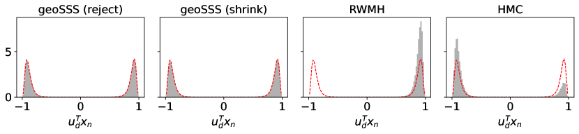
Figure 2: Histograms of approximate Bingham samples with $d=10$ and $\kappa_{d}=30$ projected on the first mode obtained with each MCMC method are shown in grey. The red dashed line indicates the baseline obtained with the acceptance/rejection sampler of [KGM18].

The insufficient sampling by RWMH and HMC results in an incorrect exploration of the modes, which should be populated equally. This is illustrated in Figure 2 which also shows the distribution of $u_{d}^{T}x$ obtained by the aforementioned acceptance/rejection method proposed in [KGM18]. The histograms obtained with the geodesic slice samplers closely match the baseline, whereas RWMH completely misses the second mode and HMC misrepresents the probability mass under the modes.

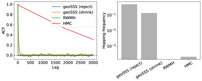
Figure 3: Left: Autocorrelation analysis of $x\mapsto u_{d}^{T}x$ with respect to approximate samples from a Bingham distribution with $d=10$ and $\kappa_{d}=30$. Right: Estimated hopping frequency between both modes of the Bingham distribution. Note that the hopping frequency is shown on a logarithmic axis.

Figure 3 shows the autocorrelation function (ACF) of $u_{d}^{T}x$ for the four MCMC samplers. We see a rapid decorrelation in case of both geodesic slice samplers; in fact, the ACF of rejection-based geoSSS drops to zero after a single step. Samples generated with RWMH decorrelate after roughly $200$ MCMC steps, but the faster decorrelation (in comparison to HMC) is due to the fact that RWMH only explores a single mode. HMC finds both modes but shows a very slowly decaying ACF, because jumps between the two modes only occur very rarely. This is also reflected in the effective sample size (ESS). Due to the immediate decorrelation of samples generated with geoSSS using a rejection strategy, the relative ESS is estimated to be 99.73 %. The shrinkage-based geoSSS obtains a relative ESS of 15.2 %, whereas RMWH and HMC achieve only very low relative ESS: 0.004 % and 0.01 %, respectively.

To quantify how rapidly the MCMC samplers mix between the two modes of the Bingham distribution, we estimated a hopping frequency, which we define as the average number of times the Markov chain jumps from one mode to the other, given by

$$\frac{1}{N-1}\sum_{n=1}^{N-1}\llbracket\text{sign}(u_{d}^{T}x_{n+1})\not=\text{sign}(u_{d}^{T}x_{n})\rrbracket,$$ (14)

where $x_{n}$ is the realization of the $n$-th Markov chain sample, $N$ the total number of steps and $\llbracket\cdot\rrbracket$ denotes the Iverson bracket.

Figure 3 shows the estimated hopping frequencies. As expected, the rejection-based geoSSS shows the highest number of oscillations between both modes with approximately 50% hopping frequency, whereas the shrinkage-based geoSSS tends to jump only every seventh step to the other mode. This behavior is expected, because the geodesic level set always contains both modes with equal probability. Therefore, the rejection sampling strategy finds each mode with equal probability, independent of what the current state of the Markov chain is. The shrinkage-based approach has a higher chance to stay in the vicinity of the current state.

Another quality measure is the geodesic or great circle distance between successive samples given as

$$\delta(x_{n+1},x_{n}):=\arccos(x_{n+1}^{T}x_{n})\,.$$

An efficient MCMC algorithm should explore the sphere rapidly by making large leaps from one sample to the next. Again, we see in Fig. 4 a superior performance of geoSSS. The RWMH algorithm achieves only small jumps. As expected, HMC moves more rapidly over the sphere compared to RWMH, but it still cannot compete with the geodesic slice samplers.

Figure 4: Geodesic distance (log-scale) between successive approximate samples for a Bingham distribution with $d=10$ and $\kappa_{d}=30$.

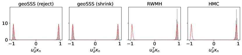
Figure S1: Histograms of approximate Bingham samples ($d=50,\kappa_{d}=300$) projected on the first mode obtained with each MCMC method are shown in grey. The red dashed line indicates the baseline obtained with the acceptance/rejection sampler of [KGM18].

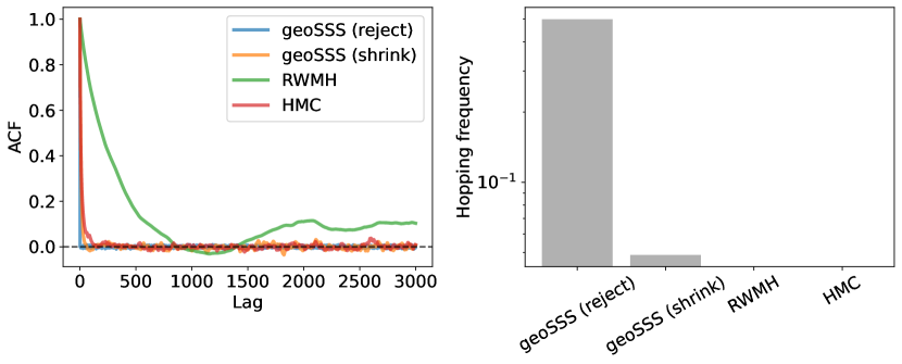
Figure S2: Left: Autocorrelation analysis of $x\mapsto u_{d}^{T}x$ with respect to approximate samples from a Bingham distribution with $d=50$ and $\kappa_{d}=300$. Right: Estimated hopping frequency between both modes of the Bingham distribution. Note that the hopping frequency is shown on a logarithmic axis.

We also run similar tests on a more challenging Bingham target with $d=50$ and $\kappa_{d}=300$, i.e., the dimension of the sample space is much larger and the distribution is more concentrated. We observe the same trends as before. Supplementary Figure S1 shows the distribution of samples projected onto the first mode. Now, both RWMH and HMC are stuck in the first mode and fail to find the second mode, whereas the geodesic slice samplers represent both modes accurately. The ACF of HMC outperforms RWMH as expected (see Supplementary Fig. S2), but still the geodesic slice samplers show a faster decorrelation than HMC resulting in a higher effective sample size. Since no jumps occur during the entire run of RWMH and HMC, their hopping frequencies are estimated to be smaller than $10^{-5}$, whereas geoSSS still achieves an acceptable jump rate (see Fig. S2). The rejection-based geoSSS clearly outperforms the shrinkage strategy on this target by achieving a higher hopping rate and as a consequence also a more favorable distribution of step sizes $\delta(x_{n+1},x_{n})$ (see Supplementary Fig. S3).

4.2. Mixture of von Mises-Fisher Distributions

We test the slice samplers as well as RWMH and HMC also on a $K$-component mixture model of von Mises-Fisher (vMF) distributions in $d$ dimensions. The vMF distribution is defined by the unnormalized density

$$p_{\text{vMF}}{}(x;\kappa,\mu)=\exp(\kappa\mu^{T}\!x),\quad x\in\mathbb{S}^{d-1},$$ (15)

where $\kappa>0$ is the concentration parameter and $\mu\in\mathbb{S}^{d-1}$. For $K\in\mathbb{N}$ our target distribution is a particular mixture of vMF distributions where each component has the same weight $1/K$ and concentration parameter $\kappa$, i.e., the corresponding unnormalized density takes the form

$$p_{\text{mix}}(x)=\frac{1}{K}\sum_{k=1}^{K}p_{\text{vMF}}(x;\kappa,\mu_{k}),\quad x\in\mathbb{S}^{d-1},$$ (16)

where every $\mu_{k}\in\mathbb{S}^{d-1}$ with $k\in\{1,\dots,K\}$ is sampled w.r.t. the uniform distribution on the unit sphere and then fixed. To generate a baseline, we use the method by Wood [Woo94].

As before, we evaluate both geoSSS variants against RWMH and HMC on a $10$-dimensional mixture of vMF distributions with $K=5$ mixture components on the unit sphere $\mathbb{S}^{9}$. We set $\kappa=100$ and draw $10^{6}$ samples.

As a measure for the quality of approximate sampling we consider the distribution with which the samplers visit the $K$ modes of the target mixture model (16). Ideally, this distribution should be uniform, because each component of the mixture has the same weight and concentration parameter. We contrast the empirical frequency $q_{k}$ with which the $k$-th mode is visited by a sampler with the uniform distribution by using the Kullback-Leibler (KL) divergence

$$\text{KL}(q\mid p):=\sum_{k=1}^{K}q_{k}\log(q_{k}/p_{k})$$

where $p_{k}=1/K$ is the ideal distribution. To estimate $q_{k}$, we assign samples $x_{n}$ to the nearest of the $K$ peaks based on the geodesic distance. This allows us to count how often each mode was visited by the Markov chain. A good MCMC sampler should produce $q_{k}\approx 1/K$ resulting in $\text{KL}(q\mid p)\approx 0$. The more the KL divergence differs from the minimum value of zero, the greater is the mismatch between the ideal and empirical frequency of mode visits. Remarkably as seen from the right panel of Fig. 5, only the geoSSS variants achieve a small KL divergence. RWMH and HMC produce large KL divergences, indicating a poorer representation of the target distribution compared to geoSSS. Although RWMH is the fastest to decorrelate (see left panel of Fig. 5), it is unreliable as observed from the KL divergence result. The geoSSS variants decorrelate much faster as compared to HMC. This aligns with the observations from the marginal histograms (see Fig. 6). Both variants of geoSSS approximates the underlying mixture significantly better compared to HMC and especially RWMH which fails to approximate every component correctly. Furthermore, the great circle distance between successive samples (see Fig. 7) shows that the slice samplers explore the entire sphere again consistent with previous numerical tests.

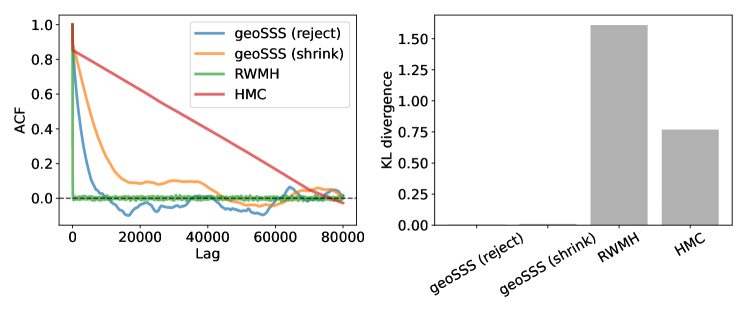
Figure 5: Left panel: ACF plotted for the first dimension from the $10$-dimensional mixture of a vMF distribution. Right panel: KL divergence between the empirical and ideal frequency with which each mode is visited by the four MCMC samplers.

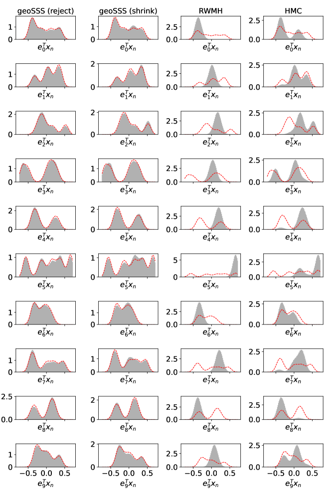
Figure 6: Marginal distributions (shown in grey) for the mixture of vMF distribution ($d=10,\kappa=100,K=5$) where columns corresponds to MCMC methods and rows correspond to the dimension of the marginal. The red dashed line indicates the baseline obtained with the acceptance/rejection sampler [Woo94].

We further evaluate the performance of the samplers by fixing the components on the sphere and increasing the concentration parameter $\kappa$ from $50$ to $500$, therefore making the distributions “spikier”. We estimate the effective sample size (ESS) for each method by considering $10$ chains and $10^{6}$ MCMC steps from the first dimension, resulting in ESS values per method for each $\kappa$. Left panel of Fig. 8 shows the estimated ESS for each of the four samplers as a function of the concentration parameter $\kappa$. Overall, we observe that sampling the mixture model becomes more challenging as the components become more concentrated with increasing $\kappa$ for all methods. However, both geoSSS outperform RWMH and HMC, particularly for lower $\kappa$ values. At large $\kappa$ values, all samplers perform similarly poorly and fail to produce a reliable approximation of the target.

Figure 7: Geodesic distance (log-scale) between successive approximate samples for the mixture of vMF distribution ($d=10$, $K=5$ and $\kappa=100$).

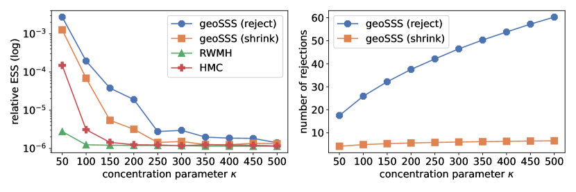
Figure 8: Comparing the MCMC samplers for the mixture of vMF distribution ($d=10$, $K=5$) by varying $\kappa$ from 50 to 500; Left panel: Considering the first dimension, estimating the relative effective sample size (ESS) for 10 chains. Right panel: Number of rejections per MCMC step.

It is worth noting that the rejection-based geoSSS yields the highest ESS, albeit at the cost of generating a significantly larger number of rejected samples in comparison to the shrinkage-based geoSSS. This is demonstrated in the right panel of Fig. 8, where it is observed that the rejection-based geoSSS generates an increasingly larger number of rejected samples for higher values of $\kappa$. For instance, for $\kappa=50$, approximately 17 rejections happen per MCMC step, while for $\kappa=500$, around 60 rejections occur. On the other hand, the number of rejections for the shrinkage-based geoSSS increases at a much slower rate with $\kappa$. It can be seen here that for $\kappa=50$, we have approximately 4 rejections per MCMC step, and for $\kappa=500$, approximately just 6 rejections per MCMC step occur. Thus, selecting between the two samplers necessitates a trade-off between computational requirements and accuracy. The number of rejections directly determines the number of log probability evaluations and thereby the computational costs of the slice samplers. RWMH and HMC, on the other hand, have a fixed computational budget per MCMC step. In case of RWMH, one step requires a single log probability evaluation, whereas an HMC step involves one log probability evaluation as well as multiple gradient evaluations, one for each leapfrog step. In our settings, we use 10 leapfrog integration steps. Among the four MCMC strategies studied here, RWMH has the lowest computational costs, but also the smallest ESS. The computational costs of shrinkage-based geoSSS is smaller than the costs of HMC, nevertheless geoSSS also performs better in terms of the other evaluation criteria in comparison to HMC.

4.3. Curved Distribution on the 2-Sphere

HMC is expected to show superior performance on target densities that accumulate ‘mass’ along narrow connected regions. To study such a sampling problem, we define a spherical distribution along a curve. The curve is created by picking 10 points uniformly distributed on the $2$-sphere and connecting them such that the overall distance is shortest (this is done by solving a small traveling salesman problem). We use spherical linear interpolation (slerp) to interpolate between two successive points $x,y\in\mathbb{S}^{d-1}$, i.e., we apply

$$t\mapsto\frac{\sin(\theta\,(1-t))x+\sin(\theta\,t)y}{\sin(\theta)},$$

where $\theta=\arccos(x^{T}y)$, c.f. [Han95]. If $\mu(t)$ with $t\in[0,1]$ is the curve obtained by concatenating the slerps between the 9 pairs of successive points, then we define the spherical distribution with unnormalized density

$$p(x)=\exp\left\{\kappa\max_{t\in[0,1]}x^{T}\!\mu(t)\right\},\qquad x\in\mathbb{S}^{d-1},$$ (17)

which we also call curved von Mises-Fisher distribution (curved vMF).

The maximum of $x^{T}\!\mu(t)$ for a single slerp can be computed in closed form. The total maximum over the entire curve is the maximum over the maxima of slerps connecting two successive points. The probability distribution determined by (17) concentrates ‘mass’ around the curve. As in the case for the standard vMF distribution, the parameter $\kappa$ controls the concentration. In our sampling tests, we choose $\kappa=300$. We run all four samplers on targeting the corresponding curved vMF. Rejection-based geoSSS and HMC takes roughly similar run duration, HMC taking slightly longer. However, almost twice as long as shrinkage-based geoSSS. RWMH is by far the fastest method. Refer Section A.11 for run times.

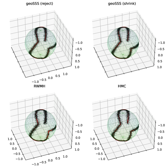
Figure 9: Samples of the four different MCMC samplers targeting a curved vMF on the $2$-sphere are shown as black dots. The red curve is generated by positioning $10$ points uniformly distributed on the sphere and interpolating between them using slerp. The concentration parameter is $\kappa=300$.

Figure 9 shows the samples of the four Markov chain approaches of the first $10000$ MCMC iterations. RWMH fails to explore the entire curve. On the other hand, the slice samplers and, as expected, HMC manage to explore the entire curve fairly uniformly. To measure the discrepancy between the discretized target and the histogram generated by a sampling procedure, we use KL divergence as a metric. Right panel of Fig. 10 shows that the two slice samplers achieve the lowest KL values, surprisingly better than HMC, and thus produce a representation of the target that is more faithful to the true distribution than what RWMH is able to achieve. RWMH also shows the worst ACF with a very slow decay (left panel Fig. 10). Among the other three samplers, the slice samplers outperform HMC in that they decorrelate more rapidly. As expected, the rejection-based geoSSS shows the fastest decorrelation. The distribution of distances between successive samples also disfavors RWMH (Fig. 11). Both geoSSS variants show a peak at very short distances. HMC performs better in that it avoids minor changes and produces larger distances. Nevertheless the slice samplers reach out to larger distances covering the entire range of great-circle distance from 0 to $\pi$ more often than HMC.

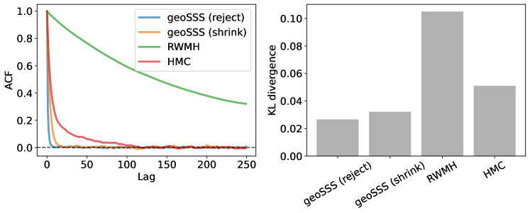
Figure 10: Left panel: ACF plotted for the first dimension based on $10^{5}$ samples. Right panel: KL divergence between a discretized version of the curved vMF target and a histogram compiled from the MCMC samples.

Figure 11: Geodesic distance (log-scale) between successive approximate samples for the curved von Mises-Fisher distribution (17).

5 Summary

We introduce two slice sampling based MCMC-methods on the sphere, the ideal geodesic and geodesic shrinkage slice samplers, that use movements on great circles. For the Markov kernels of both samplers we are able to establish reversibility under mild assumptions, and uniform ergodicity if the target density is bounded. In numerical experiments we see that in particular for moderately concentrated target distributions with a moderate number of dimensions our slice samplers perform well and can compete with RWMH and HMC on the sphere, while having the additional advantage of being free of tuning parameters. For multimodal target distributions we observe that the ideal geodesic slice sampler and the geodesic shrinkage slice sampler even outperform RWMH and HMC. However, we observe that the performance of our methods, just as for RWMH and HMC, deteriorates for increasing concentration of the target distribution, and it is to be expected that the same happens for increasing dimension. This dependence on concentration and dimension already appears in the ergodicity constants of Theorem 15 and Theorem 26. Regarding the comparison between the two geodesic slice samplers, the ideal version seems to outperform the shrinkage based sampler in terms of Markov chain transitions. However, this comes with a (significantly) greater computational cost per transition.

Code Availability

The implementation of our geoSSS algorithms as well as RWMH (see Appendix A.7) and spherical HMC [LZS14] on the sphere as well as scripts for all the numerical illustrations are compiled in our package labeled “GeoSSS”, accessible at this GitHub repository https://github.com/microscopic-image-analysis/geosss. The numerical illustration results computed from the “/scripts” directory from the repository are uploaded at Zenodo https://doi.org/10.5281/zenodo.8287302.

Appendix A Appendix

A.1. Sampling from $\frac{1}{\omega_{d-2}}\,\mu_{x}$.

Implementing the slice sampling algorithms provided in this paper involves sampling from $\frac{1}{\omega_{d-2}}\,\mu_{x}$ for $x\in\mathbb{S}^{d-1}$. Algorithm 5 describes a procedure to achieve this. We provide a proof for the validity of this algorithm.

Algorithm 5 Sampling from $\frac{1}{\omega_{d-2}}\,\mu_{x}$.

0:  point $x\in\mathbb{S}^{d-1}$

0:  sample $v$ from $\frac{1}{\omega_{d-2}}\,\mu_{x}$

1:  Draw $Y\sim\mathcal{N}(0,\mathrm{Id}_{d})$, call the result $y$.

2:  Set $z=y-({x}^{T}\!{y})\,x$.

3:  Set $v=z/\|z\|$.

Lemma 28.

Let $Y$ be a random variable distributed according to the $d$-dimensional standard normal distribution $\mathcal{N}(0,\mathrm{Id}_{d})$. Then we have

$$\frac{Y-{x}^{T}\!{\,Y}\,x}{\left\|Y-{x}^{T}\!{\,Y}\,x\right\|}\sim\frac{1}{\omega_{d-2}}\,\mu_{x},\qquad x\in\mathbb{S}^{d-1}.$$

Proof.

Let $x\in\mathbb{S}^{d-1}$. Moreover, let $U\in\mathbb{R}^{d\times(d-1)}$ be the matrix with columns $e_{1}^{(x)},\ldots,e_{d-1}^{(x)}$ and let $\widetilde{U}\in\mathbb{R}^{d\times d}$ be the matrix with columns $e_{1}^{(x)},\ldots,e_{d-1}^{(x)},x$ where $e_{1}^{(x)},\ldots,e_{d-1}^{(x)}$ are defined as in Section 2.2. Since $e_{1}^{(x)},\ldots,e_{d-1}^{(x)},x$ is an orthonormal basis of $\mathbb{R}^{d}$, we may write $y\in\mathbb{R}^{d}$ as

$$y=\sum_{i=1}^{d-1}\alpha_{i}e_{i}^{(x)}+\alpha_{d}x$$

where $\alpha\coloneqq(\alpha_{1},\dots,\alpha_{d})^{T}=\widetilde{U}^{T}y$ holds for the coefficients. Therefore, we have

$$y-{x}^{T}\!{y}\,x=\sum_{i=1}^{d-1}\alpha_{i}e_{i}^{(x)}=\varphi_{x}\left((\alpha_{1},\dots,\alpha_{d-1})^{T}\right)=\varphi_{x}(U^{T}y).$$

Since $Y\sim\mathcal{N}(0,\mathrm{Id}_{d})$ and $\widetilde{U}$ is orthogonal, also $\widetilde{U}^{T}Y\sim\mathcal{N}(0,\mathrm{Id}_{d})$. Observe that the distribution of $U^{T}Y$ is a marginal distribution of the distribution of $\widetilde{U}^{T}Y$. Hence $U^{T}Y\sim\mathcal{N}(0,\mathrm{Id}_{d-1})$. This implies $\frac{U^{T}Y}{\left\|U^{T}Y\right\|}\sim\frac{1}{\omega_{d-2}}\,\sigma_{d-2}$. Using (4) and that $\varphi_{x}$ is a linear isometry, we obtain for $A\in\mathcal{B}\left({\mathbb{S}^{d-2}_{x}}\right)$ that

$$\mathbb{P}\left(\frac{Y-{x}^{T}\!{Y}\,x}{\left\|Y-{x}^{T}\!{Y}\,x\right\|}\in A\right) =\mathbb{P}\left(\varphi_{x}\left(\frac{U^{T}Y}{\left\|U^{T}Y\right\|}\right)\in A\right)=\mathbb{P}\left(\frac{U^{T}Y}{\left\|U^{T}Y\right\|}\in\varphi_{x}^{-1}(A)\right)$$

$$=\frac{1}{\omega_{d-2}}\,\sigma_{d-2}\left(\varphi_{x}^{-1}(A)\right)=\frac{1}{\omega_{d-2}}\,\mu_{x}(A).\qed$$

A.2. Proof of Lemma 4.

We show the identities of the objects under the map $T_{\theta}$ by elementary calculations.

To (i): Using classic trigonometric identities of sine and cosine, we obtain for all $r\in\mathbb{R}$ that

$$\gamma_{T_{\theta}(x,v)}(r) =\cos(r)\big{(}\cos(\theta)x+\sin(\theta)v\big{)}+\sin(r)\big{(}\sin(\theta)x-\cos(\theta)v\big{)}$$

$$=\cos(\theta-r)x+\sin(\theta-r)v=\gamma_{(x,v)}(\theta-r).$$

To (ii): This statement is an immediate consequence of (i), since

$$\gamma_{T_{\theta}(x,v)}(\theta)=\gamma_{(x,v)}(0)=\cos(0)x+\sin(0)v=x.$$

To (iii): For $\theta\in\mathbb{R}$ set

$$w_{\theta}\colon[0,2\pi) \to[0,2\pi),\quad r\mapsto(\theta-r)\cdot\mathbbm{1}_{\theta\geq r}+(\theta-r+2\pi)\cdot\mathbbm{1}_{\theta<r}.$$

Due to the $2\pi$-periodicity of sine and cosine, we have

$$L(T_{\theta}(x,v),t)=w_{\theta}^{-1}\big{(}L(x,v,t)\big{)}.$$

Since the Lebesgue measure $\lambda_{1}$ is invariant under $w_{\theta}$, we obtain

$$\lambda_{1}\left(L(T_{\theta}(x,v),t)\right)=\lambda_{1}\left(w_{\theta}^{-1}\big{(}L(x,v,t)\big{)}\right)=\lambda_{1}\left(L(x,v,t)\right),$$

which finishes the proof.

A.3. Proof of Lemma 3.

To prove Lemma 3 we need the concept of the geodesic flow. It is defined on general Riemannian manifolds. However, we are only interested into the special case of the Euclidean unit sphere, where the expression for the geodesic flow simplifies considerably.

Definition 29.

Let $\theta\in\mathbb{R}$. The function

$$\psi_{\theta}:\mathcal{S}\mathbb{S}^{d-1} \to\mathcal{S}\mathbb{S}^{d-1}$$

$$(x,v) \mapsto\big{(}\cos(\theta)x+\sin(\theta)v,-\sin(\theta)x+\cos(\theta)v\big{)}$$

is called the geodesic flow on the sphere.

Intuitively, the geodesic flow can be thought of as moving a point $x\in\mathbb{S}^{d-1}$ and a velocity $v\in E_{x}$ for a step-size of $\theta$ along the geodesic on the sphere which is determined by $x$ and $v$.

We use the geodesic flow, because Liouville’s theorem states that the Liouville measure is invariant under the geodesic flow. This is a result which holds on general Riemannian manifolds. For convenience of the reader, we provide a formulation of it in our notation and therefore naturally restricted to the special case of the sphere.

Lemma 30 ([Cha84, Section V.2]).

For $\theta\in\mathbb{R}$ the Liouville measure as defined in (6) is invariant with respect to the geodesic flow given in Definition 29, that is,

$$\mathcal{L}\left(\psi_{\theta}^{-1}(A)\right)=\mathcal{L}(A),\quad\forall A\in\mathcal{B}\left(\mathcal{S}\mathbb{S}^{d-1}\right).$$

Proof of Lemma 3.

Let $\theta\in\mathbb{R}$ and define

$$\iota:\mathcal{S}\mathbb{S}^{d-1} \to\mathcal{S}\mathbb{S}^{d-1},\qquad(x,v)\mapsto(x,-v).$$

Observe that the Liouville measure is invariant under $\iota$, see e.g. [Pat99, Lemma 1.34]. We can express the map $T_{\theta}$ as $T_{\theta}=\iota\circ\psi_{\theta}$. Using Lemma 30 and [Pat99, Lemma 1.34] we obtain

$$\int_{\mathcal{S}\mathbb{S}^{d-1}}F\left(T_{\theta}(y)\right)\,\mathcal{L}({\rm d}y) =\int_{\mathcal{S}\mathbb{S}^{d-1}}(F\circ\iota\circ\psi_{\theta})(y)\,\mathcal{L}({\rm d}y)$$

$$=\int_{\mathcal{S}\mathbb{S}^{d-1}}(F\circ\iota)(y)\,\mathcal{L}({\rm d}y)=\int_{\mathcal{S}\mathbb{S}^{d-1}}F(y)\,\mathcal{L}({\rm d}y).\qed$$

A.4. Proof of Lemma 2.

In the following, we provide a proof for the claim that the intersection of the level sets with the geodesics have positive mass in an appropriate sense. To this end, we need the following auxiliary statement.

Lemma 31.

Let $t\in(0,\left\|p\right\|_{\infty})$. Set

$$N(t)\coloneqq\{x\in L(t)\mid\mu_{x}(V(x,t))<\omega_{d-2}\}$$

where $V(x,t)$ is defined as in Lemma 2. Then we have $\sigma_{d-1}(N(t))=0.$

Proof.

We know from Section 2.5 that $\sigma_{d-1}$ is an stationary measure of the kernel $K_{\mathcal{U}(0,2\pi)}$. We use this and (5) to rewrite $\sigma_{d-1}(L(t))$ as

$$\sigma_{d-1}(L(t)) =\int_{\mathbb{S}^{d-1}}K_{\mathcal{U}(0,2\pi)}(x,L(t))\,\sigma_{d-1}({\rm d}x)$$

$$=\int_{\mathbb{S}^{d-1}}\frac{1}{\omega_{d-2}}\int_{{\mathbb{S}^{d-2}_{x}}}\frac{1}{2\pi}\int_{[0,2\pi)}\mathbbm{1}_{L(t)}\left(\gamma_{(x,v)}(\theta)\right)\,{\rm d}\theta\,\mu_{x}({\rm d}v)\,\sigma_{d-1}({\rm d}x)$$

$$=\int_{\mathbb{S}^{d-1}}\frac{1}{\omega_{d-2}}\int_{{\mathbb{S}^{d-2}_{x}}}\frac{1}{2\pi}\int_{[0,2\pi)}\mathbbm{1}_{L(x,v,t)}\left(\theta\right)\,{\rm d}\theta\,\mu_{x}({\rm d}v)\,\sigma_{d-1}({\rm d}x)$$

$$=\frac{1}{\omega_{d-2}\ 2\pi}\int_{\mathbb{S}^{d-1}}\int_{{\mathbb{S}^{d-2}_{x}}}\lambda_{1}\big{(}L(x,v,t)\big{)}\,\mu_{x}({\rm d}v)\,\sigma_{d-1}({\rm d}x).$$

Set

$$V(t)\coloneqq\bigcup_{y\in\mathbb{S}^{d-1}}\{y\}\times V(y,t).$$

Exploiting the definitions of $V(x,t)$ and $V(t)$, we have

$$\sigma_{d-1}(L(t)) =\frac{1}{\omega_{d-2}\ 2\pi}\int_{\mathbb{S}^{d-1}}\int_{{\mathbb{S}^{d-2}_{x}}}\mathbbm{1}_{V(x,t)}(v)\lambda_{1}\big{(}L(x,v,t)\big{)}\,\mu_{x}({\rm d}v)\,\sigma_{d-1}({\rm d}x)$$

$$=\frac{1}{\omega_{d-2}\ 2\pi}\int_{\mathbb{S}^{d-1}}\int_{{\mathbb{S}^{d-2}_{x}}}\mathbbm{1}_{V(t)}(x,v)\lambda_{1}\big{(}L(x,v,t)\big{)}\,\mu_{x}({\rm d}v)\,\sigma_{d-1}({\rm d}x).$$

Lemma 3 and statement (ii) of Lemma 4 yield

$$\sigma_{d-1}(L(t))=\frac{1}{\omega_{d-2}\ 2\pi}\int_{[0,2\pi)}\int_{\mathbb{S}^{d-1}}\int_{{\mathbb{S}^{d-2}_{x}}}\mathbbm{1}_{V(t)}(x,v)\mathbbm{1}_{L(t)}\left(\gamma_{(x,v)}(\theta)\right)$$

$$\hskip 241.84842pt\,\times\mu_{x}({\rm d}v)\,\sigma_{d-1}({\rm d}x)\,{\rm d}\theta$$

$$=\frac{1}{\omega_{d-2}\ 2\pi}\int_{[0,2\pi)}\int_{\mathbb{S}^{d-1}}\int_{{\mathbb{S}^{d-2}_{x}}}\mathbbm{1}_{V(t)}\left(T_{\theta}(x,v)\right)\mathbbm{1}_{L(t)}\left(\gamma_{T_{\theta}(x,v)}(\theta)\right)$$

$$\hskip 241.84842pt\,\times\mu_{x}({\rm d}v)\,\sigma_{d-1}({\rm d}x)\,{\rm d}\theta$$

$$=\frac{1}{\omega_{d-2}\ 2\pi}\int_{[0,2\pi)}\int_{\mathbb{S}^{d-1}}\int_{{\mathbb{S}^{d-2}_{x}}}\mathbbm{1}_{V(t)}\left(T_{\theta}(x,v)\right)\mathbbm{1}_{L(t)}\left(x\right)\mu_{x}({\rm d}v)\,\sigma_{d-1}({\rm d}x)\,{\rm d}\theta.$$

Observe that statement iii of Lemma 4 and the definition of $V(t)$ directly imply $\mathbbm{1}_{V(t)}\big{(}T_{\theta}(x,v)\big{)}=\mathbbm{1}_{V(t)}(x,v)=\mathbbm{1}_{V(x,t)}(v)$. Therefore

$$\sigma_{d-1}(L(t)) =\frac{1}{\omega_{d-2}\ 2\pi}\int_{[0,2\pi)}\int_{\mathbb{S}^{d-1}}\int_{{\mathbb{S}^{d-2}_{x}}}\mathbbm{1}_{V(x,t)}(v)\mathbbm{1}_{L(t)}\left(x\right)\,\mu_{x}({\rm d}v)\,\sigma_{d-1}({\rm d}x)\,{\rm d}\theta$$

$$=\frac{1}{\omega_{d-2}}\int_{L(t)}\mu_{x}(V(x,t))\,\sigma_{d-1}({\rm d}x).$$

Now assume that $\sigma_{d-1}(N(t))>0$ would hold. Then we would have by the definition of $N(t)$ that

$$\sigma_{d-1}(L(t))$$

$$\quad=\frac{1}{\omega_{d-2}}\left(\int_{N(t)}\mu_{x}(V(x,t))\,\sigma_{d-1}({\rm d}x)+\int_{L(t)\setminus N(t)}\mu_{x}(V(x,t))\,\sigma_{d-1}({\rm d}x)\right)$$

$$\quad<\sigma_{d-1}(N(t))+\sigma_{d-1}(L(t)\setminus N(t))=\sigma_{d-1}(L(t)).$$

This is a contradiction, such that $\sigma_{d-1}(N(t))=0$. ∎

Proof of Lemma 2.

For $x\in\mathbb{S}^{d-1}$ set

$$R(x):=\{t\in(0,p(x))\mid x\in N(t)\}\subseteq\mathbb{R}_{+}.$$

Then

$$\int_{\mathbb{S}^{d-1}}\lambda_{1}(R(x))\,\sigma_{d-1}({\rm d}x) =\int_{\mathbb{S}^{d-1}}\int_{0}^{\left\|p\right\|_{\infty}}\mathbbm{1}_{N(t)}(x)\,{\rm d}t\,\sigma_{d-1}({\rm d}x)$$

$$=\int_{0}^{\left\|p\right\|_{\infty}}\sigma_{d-1}(N(t))\,{\rm d}t=0$$

due to Lemma 31. Consequently $\lambda_{1}(R(x))=0$ for $\frac{1}{\omega_{d-1}}\sigma_{d-1}$-almost all $x\in\mathbb{S}^{d-1}$. Observe that for $x\in\mathbb{S}^{d-1}$ we have

$$\{t\in(0,p(x))\mid\frac{1}{\omega_{d-2}}\,\mu_{x}(V(x,t))=1\}=(0,p(x))\setminus R(x).$$

Therefore, for $\frac{1}{\omega_{d-1}}\sigma_{d-1}$-almost all $x\in\mathbb{S}^{d-1}$ holds

$$\frac{1}{p(x)}\lambda_{1}\left(\{t\in(0,p(x))\mid\frac{1}{\omega_{d-2}}\,\mu_{x}(V(x,t))=1\}\right)=1-\frac{\lambda_{1}\left(R(x)\right)}{p(x)}=1.\quad\qed$$

A.5. Proof of Lemma 20.

The aim of this section is to give a proof of the integral estimate in Lemma 20. Note that this estimate is important for deriving the smallness of the whole state space for both slice sampling kernels on the sphere. We need the following auxiliary lemma.

Lemma 32.

Let $x\in\mathbb{S}^{d-1}$ and $A\in\mathcal{B}\left(\mathbb{S}^{d-1}\right)$. Then we have

$$\int_{0}^{\pi}\int_{{\mathbb{S}^{d-2}_{x}}}\mathbbm{1}_{A}\big{(}\gamma_{(x,v)}(\theta)\big{)}\,\mu_{x}({\rm d}v)\,{\rm d}\theta\geq\sigma_{d-1}(A).$$

To prove this statement, we make use of an expression for $\sigma_{d-1}$ in terms of polar coordinates, see [Sch17, Corollary 16.19]. Define the functions

$$f_{d-1}:(0,\pi)^{d-2}\times(-\pi,\pi) \to\mathbb{R}^{d}\setminus\{x\mid x_{d}=0,x_{d-1}\leq 0\},$$

$$(\theta_{1},\ldots,\theta_{d-1}) \mapsto\begin{pmatrix}\cos(\theta_{1})\\ \sin(\theta_{1})\cos(\theta_{2})\\ \sin(\theta_{1})\sin(\theta_{2})\cos(\theta_{3})\\ \vdots\\ \sin(\theta_{1})\cdot\ldots\cdot\sin(\theta_{d-2})\cos(\theta_{d-1})\\ \sin(\theta_{1})\cdot\ldots\cdot\sin(\theta_{d-1})\end{pmatrix},$$

$$J_{d-1}(\theta_{1},\ldots,\theta_{d-1})=\sin^{d-2}(\theta_{1})\sin^{d-3}(\theta_{2})\cdot\ldots\cdot\sin(\theta_{d-2}),$$

and

$$g:\mathbb{R}^{d}\setminus\big{\{}y\mid|y_{1}|>1\big{\}} \to\mathbb{R}_{+},\qquad(y_{1},\ldots,y_{d})\mapsto\frac{1}{\sin^{d-2}(\arccos(y_{1}))}.$$

Then for all $A\in\mathcal{B}\left(\mathbb{S}^{d-1}\right)$ we have

$$\begin{split}&\sigma_{d-1}(A)\\ &\quad=\int_{0}^{\pi}\ldots\int_{0}^{\pi}\int_{-\pi}^{\pi}\mathbbm{1}_{A}\big{(}f_{d-1}(\theta_{1},\ldots,\theta_{d-1})\big{)}J_{d-1}(\theta_{1},\ldots,\theta_{d-1})\,{\rm d}\theta_{d-1}\ldots{\rm d}\theta_{1}.\end{split}$$ (18)

Proof of Lemma 32.

Recall that $\mu_{x}=\varphi_{x}(\sigma_{d-2})$ where $\varphi_{x}$ is defined in (3). Applying (18) to $\sigma_{d-2}$ we may express

$$\int_{0}^{\pi}\int_{{\mathbb{S}^{d-2}_{x}}}\mathbbm{1}_{A}\big{(}\gamma_{(x,v)}(\theta)\big{)}\,\mu_{x}({\rm d}v)\,{\rm d}\theta=\int_{0}^{\pi}\int_{\mathbb{S}^{d-2}}\mathbbm{1}_{A}\big{(}\gamma_{(x,\varphi_{x}(y))}(\theta)\big{)}\,\sigma_{d-2}({\rm d}y)\,{\rm d}\theta$$

$$\qquad=\int_{0}^{\pi}\int_{0}^{\pi}\ldots\int_{0}^{\pi}\int_{-\pi}^{\pi}\mathbbm{1}_{A}\left(\gamma_{\left(x,\varphi_{x}\left(f_{d-2}(\theta_{1},\ldots,\theta_{d-2})\right)\right)}(\theta)\right)J_{d-2}(\theta_{1},\ldots,\theta_{d-2})$$

$$\qquad\hskip 256.0748pt\times{\rm d}\theta_{d-2}\ldots{\rm d}\theta_{1}\,{\rm d}\theta.$$

Extend the map $\varphi_{x}$ to

$$\widetilde{\varphi}_{x}:\mathbb{S}^{d-1} \to\mathbb{S}^{d-1},\qquad(y_{1},\ldots,y_{d})\mapsto y_{1}x+\sum_{i=1}^{d-1}y_{i+1}e_{i}^{(x)}.$$

Observe that

$$\gamma_{\left(x,\varphi_{x}\left(f_{d-2}(\theta_{1},\ldots,\theta_{d-2})\right)\right)}(\theta)=\widetilde{\varphi}_{x}\big{(}f_{d-1}(\theta,\theta_{1},\ldots,\theta_{d-2})\big{)}$$

and

$$J_{d-2}(\theta_{1},\ldots,\theta_{d-2})=g\big{(}f_{d-1}(\theta,\theta_{1},\ldots,\theta_{d-2})\big{)}J_{d-1}(\theta,\theta_{1},\ldots,\theta_{d-2}).$$

Therefore

$$\int_{0}^{\pi}\int_{{\mathbb{S}^{d-2}_{x}}}\mathbbm{1}_{A}\big{(}\gamma_{(x,v)}(\theta)\big{)}\,\mu_{x}({\rm d}v)\,{\rm d}\theta$$

$$=\int_{0}^{\pi}\int_{0}^{\pi}\ldots\int_{0}^{\pi}\int_{-\pi}^{\pi}\mathbbm{1}_{A}\left(\widetilde{\varphi}_{x}\big{(}f_{d-1}(\theta,\theta_{1},\ldots,\theta_{d-2})\big{)}\right)g\big{(}f_{d-1}(\theta,\theta_{1},\ldots,\theta_{d-2})\big{)}$$

$$\hskip 170.71652pt\cdot J_{d-1}(\theta,\theta_{1},\ldots,\theta_{d-2})\,{\rm d}\theta_{d-2}\ldots{\rm d}\theta_{1}\,{\rm d}\theta.$$

Applying (18) for $\sigma_{d-1}$ we obtain

$$\int_{0}^{\pi}\int_{{\mathbb{S}^{d-2}_{x}}}\mathbbm{1}_{A}\big{(}\gamma_{(x,v)}(\theta)\big{)}\,\mu_{x}({\rm d}v)\,{\rm d}\theta=\int_{\mathbb{S}^{d-1}}\mathbbm{1}_{A}\left(\widetilde{\varphi}_{x}(y)\right)g(y)\,\sigma_{d-1}({\rm d}y).$$

Observe that $0\leq\sin^{d-2}\circ\arccos\leq 1$, such that $g\geq 1$. Moreover, $\sigma_{d-1}$ is invariant under the orthogonal map $\widetilde{\varphi}_{x}$. Hence,

$$\int_{0}^{\pi}\int_{{\mathbb{S}^{d-2}_{x}}}\mathbbm{1}_{A}\big{(}\gamma_{(x,v)}(\theta)\big{)}\,\mu_{x}({\rm d}v)\,{\rm d}\theta\geq\int_{\mathbb{S}^{d-1}}\mathbbm{1}_{A}(\widetilde{\varphi}_{x}(y))\,\sigma_{d-1}({\rm d}y)=\sigma_{d-1}(A).\quad\qed$$

To prove Lemma 20, we adapt the strategy that was used by [NRS21a, Lemma 3.4] to prove smallness of compact sets for the elliptical slice sampler to our setting and combine it with Lemma 32.

Proof of Lemma 20.

Let $x\in\mathbb{S}^{d-1}$. Observe that for all $v\in{\mathbb{S}^{d-2}_{x}}$ and $\theta\in[0,2\pi)$ with $\gamma_{(x,v)}(\theta)\in C$ holds

$$\frac{1}{p(x)}\int_{0}^{p(x)}\mathbbm{1}_{\left[0,p\left(\gamma_{(x,v)}(\theta)\right)\right]}(t)\,{\rm d}t=\min\left\{1,\frac{p\left(\gamma_{(x,v)}(\theta)\right)}{p(x)}\right\}\geq\frac{\inf_{y\in C}p(y)}{\sup_{y\in\mathbb{S}^{d-1}}p(y)}=\beta.$$

Therefore for $A\in\mathcal{B}\left(\mathbb{S}^{d-1}\right)$ we have

$$\frac{1}{p(x)}\int_{0}^{p(x)}\int_{{\mathbb{S}^{d-2}_{x}}}\int_{L(x,v,t)}\mathbbm{1}_{A}\big{(}\gamma_{(x,v)}(\theta)\big{)}\ {\rm d}\theta\,\mu_{x}({\rm d}v)\,{\rm d}t$$

$$\qquad\geq\frac{1}{p(x)}\int_{0}^{p(x)}\int_{{\mathbb{S}^{d-2}_{x}}}\int_{L(x,v,t)}\mathbbm{1}_{A\cap C}\big{(}\gamma_{(x,v)}(\theta)\big{)}\ {\rm d}\theta\,\mu_{x}({\rm d}v)\,{\rm d}t$$

$$\qquad=\int_{{\mathbb{S}^{d-2}_{x}}}\int_{0}^{2\pi}\mathbbm{1}_{A\cap C}\big{(}\gamma_{(x,v)}(\theta)\big{)}\cdot\frac{1}{p(x)}\int_{0}^{p(x)}\mathbbm{1}_{\left[0,p\left(\gamma_{(x,v)}(\theta)\right)\right]}(t)\,{\rm d}t\,{\rm d}\theta\,\mu_{x}({\rm d}v)$$

$$\qquad\geq\beta\int_{{\mathbb{S}^{d-2}_{x}}}\int_{0}^{\pi}\mathbbm{1}_{A\cap C}\big{(}\gamma_{(x,v)}(\theta)\big{)}\,{\rm d}\theta\,\mu_{x}({\rm d}v).$$

Applying Lemma 32 yields

$$\frac{1}{p(x)}\int_{0}^{p(x)}\int_{{\mathbb{S}^{d-2}_{x}}}\int_{L(x,v,t)}\mathbbm{1}_{A}\big{(}\gamma_{(x,v)}(\theta)\big{)}\ {\rm d}\theta\,\mu_{x}({\rm d}v)\,{\rm d}t\geq\beta\,\sigma_{d-1}(A\cap C).\qquad\quad\qed$$

A.6. Proof of Lemma 24.

In [HNR23] a formal description, with a reversibility result, of the shrinkage scheme is provided. The shrinkage procedure of the geodesic shrinkage slice sampler fits into the framework considered in there, such that we may use the aforementioned reversibility in the proof of Lemma 24. For convenience of the reader we restate the description of the shrinkage procedure from [HNR23] and state the corresponding reversibility result. To this end we call a set $S\in\mathcal{B}\left([0,2\pi)\right)$ open in $\mathbb{S}^{1}$ if for all $\theta\in S$ there exists $\varepsilon>0$ such that $\{a\mod 2\pi\mid|a-\theta|<\varepsilon,a\in\mathbb{R}\}\subseteq S$.

Algorithm 6 Algorithm 2.2 from [HNR23] with input $S\in\mathcal{B}\left([0,2\pi)\right)$ and $\theta\in S$, called by $\overline{\text{shrink}}(\theta,S)$.

input:  current state $\theta\in S$

1:  Set $i:=1$ and draw $\Lambda_{i}\sim\mathcal{U}(0,2\pi)$, call the result $a_{i}$.

2:  Set $a^{\min}_{i}:=a_{i}$ and $a_{i}^{\max}:=a_{i}$.

3:  while $a_{i}\notin S$ do

4:     if  $a_{i}\in I(a^{\min}_{i},\theta)$ then

5:        Set $a^{\min}_{i+1}:=a_{i}$ and $a^{\max}_{i+1}:=a^{\max}_{i}$.

6:     else

7:        Set $a^{\min}_{i+1}=a^{\min}_{i}$ and $a^{\max}_{i+1}=a_{i}$.

8:     end if

9:     Draw $\Lambda_{i+1}\sim\mathcal{U}(a^{\min}_{i+1},a^{\max}_{i+1})$, call the result $a_{i+1}$.

10:     Set $i:=i+1$.

11:  end while

output:  step-size $a_{i}$

For $a,b\in[0,2\pi)$ define generalized intervals

$$I(a,b):=\begin{dcases}[0,b)\cup[a,2\pi),&a\geq b\\ [a,b),&a<b.\end{dcases}$$

For a given set $S\in\mathcal{B}\left([0,2\pi)\right)$ that is open in $\mathbb{S}^{1}$ the transition kernel defined by Algorithm 6 is denoted by

$$\bar{Q}_{S}:S\times\mathcal{B}\left(S\right)\to[0,1],$$ (19)

that is,

$$\bar{Q}_{S}(\theta,A)=\mathbb{P}\big{(}\overline{\text{shrink}}(\theta,S)\in A\big{)},\qquad\forall\theta\in[0,2\pi),A\in\mathcal{B}\left([0,2\pi)\right).$$

Observe that for $S=L(x,v,t)$, $x\in\mathbb{S}^{d-1}$, $v\in{\mathbb{S}^{d-2}_{x}}$ and $t\in\mathbb{R}_{+}$, holds

$$\begin{split}Q_{{x,}{v,}{t}}(\cdot)&=\mathbb{P}\big{(}\text{shrink}(x,v,t)\in\cdot\big{)}=\mathbb{P}\big{(}\overline{\text{shrink}}(0,L(x,v,t))\in\cdot\big{)}\\ &=\bar{Q}_{L(x,v,t)}(0,\cdot),\end{split}$$ (20)

where the distribution $Q_{{x,}{v,}{t}}$ is provided in Definition 21. We state two useful properties of the kernel of the shrinkage procedure $\bar{Q}_{S}$ that are proven in [HNR23].

Lemma 33 ([HNR23, Theorem 2.9]).

Let $S\in\mathcal{B}\left([0,2\pi)\right)$ be open in $\mathbb{S}^{1}$. Then the kernel $\bar{Q}_{S}$ defined in (19) is reversible with respect to the uniform distribution $\mathcal{U}(S)$ on $S$.

Lemma 34 ([HNR23, Lemma 2.10]).

Let $S\in\mathcal{B}\left([0,2\pi)\right)$ be open in $\mathbb{S}^{1}$, $\theta\in[0,2\pi)$, and define

$$g_{\theta}:[0,2\pi)\to[0,2\pi),\qquad a\mapsto(\theta-a)\ \text{mod}\ 2\pi.$$

Then

$$\bar{Q}_{g_{\theta}^{-1}(S)}\left(0,g_{\theta}^{-1}(A)\right)=\bar{Q}_{S}(\theta,A),\qquad\forall A\in\mathcal{B}\left(S\right).$$

By Lemma 4 statement (i) and the $2\pi$-periodicity of sine and cosine, we have

$$\gamma_{(x,y)}\left(g_{\theta}(a)\right)=\gamma_{T_{\theta}(x,v)}(a),\qquad\forall\ x\in\mathbb{S}^{d-1},v\in{\mathbb{S}^{d-2}_{x}},\theta,a\in[0,2\pi),$$

where $g_{\theta}$ is defined as in the previous lemma. This yields

$$g_{\theta}^{-1}\big{(}L(x,v,t)\big{)}=L(T_{\theta}(x,v),t)\qquad\text{and}\qquad g_{\theta}^{-1}\left(\gamma_{(x,v)}^{-1}(B)\right)=\gamma_{T_{\theta}(x,v)}^{-1}(B)$$

for all $B\in\mathcal{B}\left(\mathbb{S}^{d-1}\right)$. Hence, by applying Lemma 34 for $A=\gamma_{(x,v)}^{-1}(B)$ and $S=L(x,v,t)$, we obtain

$$\begin{split}\bar{Q}_{L(T_{\theta}(x,v),t)}\left(0,\gamma_{T_{\theta}(x,v)}^{-1}(B)\right)&=\bar{Q}_{g_{\theta}^{-1}\big{(}L(x,v,t)\big{)}}\left(0,g_{\theta}^{-1}\left(\gamma_{(x,v)}^{-1}(B)\right)\right)\\ &=\bar{Q}_{L(x,v,t)}(\theta,\gamma_{(x,v)}^{-1}(B))\end{split}$$ (21)

for all $x\in\mathbb{S}^{d-1},v\in{\mathbb{S}^{d-2}_{x}},\theta\in[0,2\pi),t>0$ and $B\in\mathcal{B}\left(\mathbb{S}^{d-1}\right)$.

Remark 35.

We comment on the strategy of proof for Lemma 24. We obtain the statement by applying Lemma 13. This means we need to show that $\widetilde{H}_{t}$ is reversible with respect to $\frac{1}{\sigma_{d-1}(L(t))}\,\sigma_{d-1}|_{L(t)}$ for all $t\in(0,\left\|p\right\|)_{\infty}$. We achieve this by using the invariance of the Liouville measure $\mathcal{L}$ under the map $T_{\theta}$ (see Lemma 3) and Lemma 33.

Proof of Lemma 24.

Let $t\in(0,\left\|p\right\|_{\infty})$ and $A,B\in\mathcal{B}\left(\mathbb{S}^{d-1}\right)$. Due to the lower-semicontinuity of $p$, the level set $L(t)$ is open. Thus, $L(x,v,t)$ is open in $\mathbb{S}^{1}$ for all $x\in L(t)$ and $v\in{\mathbb{S}^{d-2}_{x}}$. Additionally $x\in L(t)$ implies that $L(x,v,t)$ is also non-empty, such that

$$\lambda_{1}\big{(}L(x,v,t)\big{)}>0,\qquad\forall\ x\in L(t),v\in{\mathbb{S}^{d-2}_{x}}.$$

Hence, we have, exploiting (20), that

$$\omega_{d-2}\int_{B\cap L(t)}\widetilde{H}_{t}(x,A)\,\sigma_{d-1}({\rm d}x)$$

$$=\int_{B\cap L(t)}\int_{{\mathbb{S}^{d-2}_{x}}}\bar{Q}_{L(x,v,t)}(0,\gamma_{(x,v)}^{-1}(A))\,\mu_{x}({\rm d}v)\,\sigma_{d-1}({\rm d}x)$$

$$=\int_{[0,2\pi)}\int_{B\cap L(t)}\int_{{\mathbb{S}^{d-2}_{x}}}\frac{\mathbbm{1}_{L(x,v,t)}(\theta)}{\lambda_{1}(L(x,v,t))}\bar{Q}_{L(x,v,t)}(0,\gamma_{(x,v)}^{-1}(A))\mu_{x}({\rm d}v)\,\sigma_{d-1}({\rm d}x)\,{\rm d}\theta.$$

Then, Lemma 3 yields

$$\omega_{d-2}\int_{B\cap L(t)}\widetilde{H}_{t}(x,A)\,\sigma_{d-1}({\rm d}x)$$

$$\qquad=\int_{[0,2\pi)}\int_{\mathbb{S}^{d-1}}\int_{{\mathbb{S}^{d-2}_{x}}}\mathbbm{1}_{B\cap L(t)}\left(\gamma_{(x,v)}(\theta)\right)\frac{\mathbbm{1}_{L(T_{\theta}(x,v),t)}(\theta)}{\lambda_{1}(L(T_{\theta}(x,v),t))}$$

$$\quad\hskip 128.0374pt\times\bar{Q}_{L(T_{\theta}(x,v),t)}(0,\gamma_{T_{\theta}(x,v)}^{-1}(A))\ \mu_{x}({\rm d}v)\,\sigma_{d-1}({\rm d}x)\,{\rm d}\theta.$$

Using (21), (5) and Lemma 4, we obtain

$$\omega_{d-2}\int_{B\cap L(t)}\widetilde{H}_{t}(x,A)\,\sigma_{d-1}({\rm d}x)$$

$$=\int_{[0,2\pi[}\int_{\mathbb{S}^{d-1}}\int_{{\mathbb{S}^{d-2}_{x}}}\mathbbm{1}_{B}(\gamma_{(x,v)}(\theta))\mathbbm{1}_{L(x,v,t)}(\theta)\frac{\mathbbm{1}_{L(t)}(x)}{\lambda_{1}(L(x,v,t))}\bar{Q}_{L(x,v,t)}(\theta,\gamma_{(x,v)}^{-1}(A))$$

$$\hskip 270.30118pt\times\mu_{x}({\rm d}v)\,\sigma_{d-1}({\rm d}x)\,{\rm d}\theta$$

$$=\int_{L(t)}\int_{{\mathbb{S}^{d-1}_{x}}}\frac{1}{\lambda_{1}(L(x,v,t))}\int_{\gamma_{(x,v)}^{-1}(B)\cap L(x,v,t)}\bar{Q}_{L(x,v,t)}(\theta,\gamma_{(x,v)}^{-1}(A))$$

$$\hskip 270.30118pt\times{\rm d}\theta\,\mu_{x}({\rm d}v)\,\sigma_{d-1}({\rm d}x).$$

As $L(x,v,t)$ is open in $\mathbb{S}^{1}$ for all $x\in L(t)$ and $v\in{\mathbb{S}^{d-2}_{x}}$, we may apply Lemma 33 and get

$$\omega_{d-2}\int_{B\cap L(t)}\widetilde{H}_{t}(x,A)\,\sigma_{d-1}({\rm d}x)$$

$$\quad=\int_{L(t)}\int_{{\mathbb{S}^{d-1}_{x}}}\frac{1}{\lambda_{1}(L(x,v,t))}\int_{\gamma_{(x,v)}^{-1}(A)\cap L(x,v,t)}\bar{Q}_{L(x,v,t)}(\theta,\gamma_{(x,v)}^{-1}(B))$$

$$\quad\hskip 250.38434pt\times{\rm d}\theta\,\mu_{x}({\rm d}v)\,\sigma_{d-1}({\rm d}x).$$

Performing the same arguments in reversed order, we get

$$\omega_{d-2}\int_{B\cap L(t)}\widetilde{H}_{t}(x,A)\,\sigma_{d-1}({\rm d}x)=\omega_{d-2}\int_{A\cap L(t)}\widetilde{H}_{t}(x,B)\,\sigma_{d-1}({\rm d}x).$$

Thus, by Lemma 13, we obtain reversibility of $\widetilde{H}$ with respect to $\pi$. ∎

A.7. Random-walk Metropolis-Hastings on the Sphere.

The random-walk Metropolis-Hastings (RWMH) algorithm uses an isotropic Gaussian proposal kernel. As suggested in [LRSS22], for current state $x\in\mathbb{S}^{d-1}$ we choose an auxiliary point $\sqrt{r}x$ in the ambient space $\mathbb{R}^{d}$ by generating a radius $\sqrt{r}$, with $r$ being a realization of

$$R\sim{\rm Gamma}(d/2,1/2)\,.$$

Then, given $\sqrt{r}x$ we sample a realization $y$ from

$$Y\sim{\rm Normal}\left(rx,\varepsilon^{2}\mathrm{Id}_{d}\right),$$

where $\varepsilon$ is the step-size of the random walk. Since this $y$ does not yet lie on the sphere, we radially project and propose $y/\|y\|$, which finally is accepted or rejected using the usual acceptance ratio. In Algortihm 7 we provide the corresponding pseudocode.

Algorithm 7 Reprojected RWMH on $\mathbb{S}^{d-1}$ for step-size $\varepsilon>0$.

input: current state $x\in\mathbb{S}^{d-1}$
output: next state $x^{\prime}$

1:  Draw $R\sim{\rm Gamma}\left(d/2,1/2\right)$, call the result $r$.

2:  Draw $Y\sim{\rm Normal}\left(\sqrt{r}\,x,\varepsilon^{2}\mathrm{Id}_{d}\right)$, call the result $y$.

3:  Set $z=y/\|y\|$.

4:  Draw $U\sim\mathcal{U}(0,1)$, call the result $u$.

5:  if $u\leq\min\left\{1,p(z)/p(x)\right\}$ then

6:     $x^{\prime}=z$

7:  else

8:     $x^{\prime}=x$

9:  end if

A.8. Hamiltonian Monte Carlo on the Sphere.

Since RWMH suffers from diffusive behavior, we also test spherical Hamiltonian Monte Carlo (HMC) suggested in [LZS14] as an alternative MCMC approach. In spherical HMC, the sample space is first augmented by momenta or velocities $v\in\mathbb{R}^{d}$ that are in the the tangent space $E_{x}$ to $\mathbb{S}^{d-1}$ at the current sample $x$. The momenta follow a standard Normal distribution, and the Markov chain is generated in the space $\{(x,v)\mid x\in\mathbb{S}^{d-1},v\in E_{x}\}$. Diffusive behavior is suppressed by the special type of proposal step that solves Hamilton’s equations of motion by using a leapfrog integrator [Nea11]. During leapfrog integration, the gradient of the log probability $\nabla\log p(x)$ guides the Markov chain, thereby reaching nearby modes in much shorter time than RWMH. The spherical HMC algorithm is detailed in Algorithm 8. In contrast to standard HMC, spherical HMC involves a rotation of the positions and momenta during leapfrog integration where the rotation matrix is a Givens rotation $G(v/\|v\|,x,\theta)$ in the plane spanned by the momenta $v$ and the positions $x$ (see lines 8–10 in Algorithm 8 and (8)). In addition to the step-size parameter $\varepsilon>0$, we also need to choose the number of leapfrog steps $T\in\mathbb{N}$. In our experiments, we always set $T=10$.

A.9. Step-size Tuning for RWMH and HMC

Both RWMH and spherical HMC involve a step-size parameter $\varepsilon$. Because a good choice of $\varepsilon$ depends on the particular shape of our target distribution $p(x)$, we first find $\varepsilon$ automatically during a burn-in phase. During burn-in, we increase $\varepsilon$ by a factor 1.02, if the proposal (based on the current value of $\varepsilon$) is accepted. We decrease $\varepsilon$ by a factor 0.98 if the proposed state is rejected. After a burn-in phase, the value of $\varepsilon$ is kept fixed.

Algorithm 8 Hamiltonian Monte Carlo on $\mathbb{S}^{d-1}$ for step-size $\varepsilon>0$ and number of integration steps $T$ .

input: current state $x\in\mathbb{S}^{d-1}$
output: next state $x^{\prime}$

1:  Draw $V\sim{\rm Normal}(0,\mathrm{Id}_{d})$, call the result $v$.

2:  Set $v_{1}=(\mathrm{Id}_{d}-xx^{T})\,v$.

3:  Set $x_{1}=x$.

4:  Set $t=1$.

5:  while $t\leq T$ do

6:     Set $v_{t+1/2}=v_{t}+\frac{\varepsilon}{2}\,\left(\mathrm{Id}_{d}-x_{t}x_{t}^{T}\right)\,\nabla\log p(x_{t})$.

7:     Set $R=G(v_{t+1/2}/\|v_{t+1/2}\|,x_{t},\varepsilon\,\|v_{t+1/2}\|)$.

8:     Set $x_{t+1}=R\,x_{t}$.

9:     Set $v_{t+1}=R\,v_{t+1/2}+\frac{\varepsilon}{2}\,\left(\mathrm{Id}_{d}-x_{t+1}x_{t+1}^{T}\right)\,\nabla\log p(x_{t+1})$.

10:     Set $t:=t+1$.

11:  end while

12:  Draw $U\sim\mathcal{U}(0,1)$, call the result $u$.

13:  if $u<\min\left\{1,\exp\left(\|v_{1}\|^{2}/2-\|v_{T}\|^{2}/2\right)\,{p(x_{T})}/{p(x)}\right\}$ then

14:     Set $x^{\prime}=x_{T}$.

15:  else

16:     Set $x^{\prime}=x$.

17:  end if

A.10. Tests on 50-dimensional Bingham Distribution.

Tests for the 50-dimensional Bingham distribution with a concentration parameter $\kappa_{50}=300$.

Figure S3: Geodesic distance (log-scale) between successive approximate samples for a Bingham distribution with $d=50$ and $\kappa_{d}=300$.

A.11. Run Times of Numerical Illustrations

We summarize the run times in seconds (s) for all the numerical experiments tested on Intel i7-10510U CPU in Table 1. We nomenclate these experiments for brevity. For the Bingham distribution with $d=10$, $\kappa_{d}=30$ and $N=10^{5}$ as “Bingham-d10”, for the Bingham distribution with $d=50$, $\kappa_{d}=300$ and $N=10^{5}$ as “Bingham-d50”, for the mixture of vMF distribution with $d=10$, $\kappa=100$, $K=5$ and $N=10^{6}$ as “vMF-d10” and for the curve vMF distribution with $\kappa=300$ and $N=10^{5}$ as “curved-vMF”.

Numerical	MCMC Methods
Illustrations	geoSSS (reject)	geoSSS (shrink)	RWMH	HMC
Bingham-d10	13.9 s	8.5 s	3.5 s	28.4 s
Bingham-d50	36.5 s	13.1 s	3.5 s	32.0 s
vMF-d10	2601.6 s	812.9 s	274.4 s	1898.9 s
curved-vMF	926.6 s	419.5 s	151.4 s	1008.1 s

Table 1: Comparison of run times for each MCMC method across different numerical illustrations.

References

• [BG13] Simon Byrne and Mark Girolami, Geodesic Monte Carlo on embedded manifolds, Scandinavian Journal of Statistics 40 (2013), no. 4, 825–845.
• [BK22] Alexandros Beskos and Kengo Kamatani, MCMC algorithms for posteriors on matrix spaces, Journal of Computational and Graphical Statistics 31 (2022), no. 3, 721–738.
• [Boo86] William M. Boothby, An introduction to differentiable manifolds and Riemannian geometry, second ed., Pure and Applied Mathematics, vol. 120, Academic Press, Inc., Orlando, FL, 1986.
• [BRS93] Claude J. P. Bélisle, H. Edwin Romeijn, and Robert L. Smith, Hit-and-run algorithms for generating multivariate distributions, Mathematics of Operations Research 18 (1993), no. 2, 255–266.
• [Cha84] Isaac Chavel, Eigenvalues in Riemannian geometry, Pure and Applied Mathematics, vol. 115, Academic Press, Inc., Orlando, FL, 1984.
• [Giv58] Wallace Givens, Computation of plain unitary rotations transforming a general matrix to triangular form, Journal of the Society for Industrial and Applied Mathematics 6 (1958), no. 1, 26–50.
• [GS19] Navin Goyal and Abhishek Shetty, Sampling and optimization on convex sets in Riemannian manifolds of non-negative curvature, Proceedings of the Thirty-Second Conference on Learning Theory, vol. 99, PMLR, 2019, pp. 1519–1561.
• [Han95] Andrew J. Hanson, Rotations for N-dimensional graphics, Graphics Gems V, Elsevier, 1995, pp. 55–64.
• [Has70] Wilfred K. Hastings, Monte Carlo sampling methods using Markov chains and their applications, Biometrika 57 (1970), no. 1, 97–109.
• [Hir21] Osamu Hirose, A bayesian formulation of coherent point drift, IEEE Transactions on Pattern Analysis and Machine Intelligence 43 (2021), no. 7, 2269–2286.
• [HLSS20] Andrew Holbrook, Shiwei Lan, Jeffrey Streets, and Babak Shahbaba, Nonparametric Fisher geometry with application to density estimation, Proceedings of the 36th Conference on Uncertainty in Artificial Intelligence (UAI), vol. 124, PMLR, 2020, pp. 101–110.
• [HNR23] Mareike Hasenpflug, Viacheslav Natarovskii, and Daniel Rudolf, Reversibility of elliptical slice sampling revisited, arXiv: 2301.02426v1, 2023.
• [HSSW22] Michael Herrmann, Simon Schwarz, Anja Sturm, and Max Wardetzky, Efficient random walks on Riemannian manifolds, arXiv:2022.00959v1, 2022.
• [Kac56] Marc Kac, Foundations of kinetic theory, Proceedings of the Third Berkeley Symposium on Mathematical Statistics and Probability, vol. 3, University of California Press, 1956, pp. 171–197.
• [KGM18] John T. Kent, Asaad M. Ganeiber, and Kanti V. Mardia, A new unified approach for the simulation of a wide class of directional distributions, Journal of Computational and Graphical Statistics 27 (2018), no. 2, 291–301.
• [ŁR14] Krzysztof Łatuszyński and Daniel Rudolf, Convergence of hybrid slice sampling via spectral gap, arXiv: 1409.2709v1, 2014.
• [LRSS22] Han C. Lie, Daniel Rudolf, Björn Sprungk, and Timothy J. Sullivan, Dimension-independent Markov chain Monte Carlo on the sphere, arXiv:2112.12185v2, 2022.
• [LV18] Yin Tat Lee and Santosh S. Vempala, Convergence rate of Riemannian Hamiltonian Monte Carlo and faster polytope volume computation, Proceedings of the 50th Annual ACM SIGACT Symposium on Theory of Computing, Association for Computing Machinery, 2018, p. 1115–1121.
• [LZS14] Shiwei Lan, Bo Zhou, and Babak Shahbaba, Spherical Hamiltonian Monte Carlo for constrained target distributions, Proceedings of the 31st International Conference on Machine Learning, vol. 32, PMLR, 2014, pp. 629–637.
• [MAM10] Iain Murray, Ryan Adams, and David MacKay, Elliptical slice sampling, Proceedings of the thirteenth International Conference on Artificial Intelligence and Statistics, vol. 9, PMLR, 2010, pp. 541–548.
• [MJ00] Kanti V. Mardia and Peter E. Jupp, Directional statistics, John Wiley & Sons, Ltd., Chichester, 2000.
• [MMFK22] Augustin Marignier, Jason D. McEwen, Ana M. G. Ferreira, and Thomas D. Kitching, Posterior sampling for inverse imaging problems on the sphere in seismology and cosmology, arXiv: 2107.06500v3, 2022.
• [MN07] Peter Mathé and Erich Novak, Simple Monte Carlo and the Metropolis algorithm, Journal of Complexity 23 (2007), no. 4, 673–696.
• [MS18] Oren Mangoubi and Aaron Smith, Rapid mixing of geodesic walks on manifolds with positivecurvature, The Annals of Applied Probability 28 (2018), no. 4, 2501–2543.
• [MT09] Sean Meyn and Richard L. Tweedie, Markov chains and stochastic stability, second ed., Cambridge University Press, Cambridge, 2009.
• [Mun91] James R. Munkres, Analysis on manifolds, Addison-Wesley Publishing Company, 1991.
• [Nea03] Radford M. Neal, Slice sampling, The Annals of Statistics 31 (2003), no. 3, 705–767.
• [Nea11]  , MCMC using Hamiltonian dynamics, Handbook of Markov Chain Monte Carlo (2011), 113–162.
• [NRS21a] Viacheslav Natarovskii, Daniel Rudolf, and Björn Sprungk, Geometric convergence of elliptical slice sampling, Proceedings of the 38th International Conference on Machine Learning, vol. 139, PMLR, 2021, pp. 7969–7978.
• [NRS21b]  , Quantitative spectral gap estimate and Wasserstein contraction of simple slice sampling, The Annals of Applied Probability 31 (2021), no. 2, 806 – 825.
• [Pat99] Gabriel P. Paternain, Geodesic flows, Prog. Math., vol. 180, Boston, MA: Birkhäuser, 1999 (English).
• [Pet16] Peter Petersen, Riemannian geometry, third ed., Graduate Texts in Mathematics, vol. 171, Springer, Cham, 2016.
• [PS17] Natesh S. Pillai and Aaron Smith, Kac’s walk on $n$-sphere mixes in $n\log n$ steps, The Annals of Applied Probability 27 (2017), no. 1, 631–650.
• [RS22] Joel W. Robbin and Dietmar A. Salamon, Introduction to differential geometry, Springer Spektrum Berlin, Heidelberg, 2022.
• [Sch17] René L. Schilling, Measures, integrals and martingales, second ed., Cambridge University Press, Cambridge, 2017.
• [SK97] Edward .B Saff and Amo B. J. Kuijlaars, Distributing many points on a sphere, The mathematical intelligencer 19 (1997), 5–11.
• [Woo94] Andrew T. A. Wood, Simulation of the von Mises Fisher distribution, Communications in Statistics - Simulation and Computation 23:1 (1994), 157–164.
• [YŁR22] Jun Yang, Krzysztof Łatuszyński, and Gareth O. Roberts, Stereographic Markov Chain Monte Carlo, arXiv:2205.12112v1, 2022.