Photometric Calibrations of M-dwarf Metallicity with Markov Chain Monte Carlo and Bayesian Inference

Abstract

Knowledge of stellar atmospheric parameters ($T_{\rm eff}$, $\log{g}$, [Fe/H]) of M dwarfs can be used to constrain both theoretical stellar models and Galactic chemical evolutionary models, and guide exoplanet searches, but their determination is difficult due to the complexity of the spectra of their cool atmospheres. In our ongoing effort to characterize M dwarfs, and in particular their chemical composition, we carried out multiband photometric calibrations of metallicity for early- and intermediate-type M dwarfs. The third Gaia data release provides high-precision astrometry and three-band photometry. This information, combined with the 2MASS and CatWISE2020 infrared photometric surveys and a sample of 4919 M dwarfs with metallicity values determined with high-resolution spectroscopy by The Cannon and APOGEE spectra, allowed us to study the effect of the metallicity in color–color and color–magnitude diagrams. We divided this sample into two subsamples: we used 1000 stars to train the calibrations with Bayesian statistics and Markov Chain Monte Carlo techniques, and the remaining 3919 stars to check the accuracy of the estimations. We derived several photometric calibrations of metallicity applicable to M dwarfs in the range of $-0.45\leq\text{[Fe/H]}\leq+0.45$ dex and spectral types down to M5.0 V that yield uncertainties down to the $0.10$ dex level. Lastly, we compared our results with other photometric estimations published in the literature for an additional sample of 46 M dwarfs in wide binary systems with FGK-type primary stars, and found a great predictive performance.

1 Introduction

M-type dwarf stars are the coolest, smallest, and most numerous main-sequence stars in the Galaxy, with effective temperatures of $3900\,\text{K}\gtrsim T_{\rm eff}\gtrsim 2300\,\text{K}$, radii of $0.61\,R_{\odot}\gtrsim R\gtrsim 0.10\,R_{\odot}$, and masses of $0.62\,M_{\odot}\gtrsim M\gtrsim 0.08\,M_{\odot}$ (Delfosse et al., 2000; Schweitzer et al., 2019; Cifuentes et al., 2020). These stars are so faint that, despite dominating in number the solar neighborhood, none of them is visible to the naked eye (Croswell, 2002). These stars are also characterized by very active chromospheres and coronae (West et al., 2008; Jeffers et al., 2018; Kiman et al., 2021).

M dwarfs are objects of special interest in multiple branches of astrophysics. These stars have main-sequence lifetimes that exceed the currently known age of the universe, due to the slow fusion process in their mainly convective interiors (Adams & Laughlin, 1997), and they are the most abundant main-sequence stars in the Milky Way, accounting for more than 75 % of them (Henry et al., 2006; Winters et al., 2015; Reylé et al., 2021). Therefore, M dwarfs stand as excellent probes to study the chemical and dynamical evolution of our Galaxy (Bahcall & Soneira, 1980; Reid et al., 1997; Chabrier, 2003; Ferguson et al., 2017).

Despite the considerable progress with the modeling of stellar spectra over the last decades, there are still disagreements between the observational characteristics of M dwarfs and the values predicted by synthetic spectra. For instance, effective temperatures ($T_{\text{eff}}$) from models can be up to 200–300 K hotter than observed values, while radii predictions differ from interferometric measurements by up to 25 % (Jones et al., 2005; Sarmento et al., 2020). These deviations may be due to effects caused by the level of activity (López-Morales & Ribas, 2005), differences in metallicity (Berger et al., 2006; López-Morales, 2007), or the synthetic gap (Passegger et al., 2020, 2022). Additionally, there are several complications in the model atmospheres of late-type stars. For example, stellar convection in M dwarfs challenges some of the physical assumptions for radiative transfer (Bergemann et al., 2017; Olander et al., 2021) and there is an incompleteness regarding the line lists and atomic parameters used (Shetrone et al., 2015).

Furthermore, the two most successful techniques for detecting exoplanets, namely the radial velocity and transit methods, are favored in M dwarfs (Nutzman & Charbonneau, 2008; Engle & Guinan, 2011; Shields et al., 2016; Reiners et al., 2018). The lower masses of these stars facilitate the detection of exoplanets by analyzing their radial velocity curves and, due to their faintness, their habitable zone is located much closer to the star than for solar-type stars (Tarter et al., 2007; Kopparapu et al., 2014; Martínez-Rodríguez et al., 2019). This closeness translates into much shorter orbital periods of the exoplanets in the habitable zone, which makes their detection by the transit method much easier. There are several programs focused on finding exoplanets around M dwarfs. On the one hand, there are transit surveys both from the ground (e.g. MEarth; Irwin et al., 2015) and space (TESS; Ricker et al., 2014), including several JWST (Gardner et al., 2006) Guaranteed Time Observations (GTO) programs focused on exoplanets. On the other hand, there are several ground-based radial velocity instruments such as ESPRESSO (Pepe et al. 2010, 2021), HARPS (Mayor et al. 2003), HARPS-N (Cosentino et al. 2012), HPF (Mahadevan et al. 2012), IRD (Kotani et al. 2018), MAROON-X (Seifahrt et al. 2020), NEID (Schwab et al. 2016), or CARMENES (Alonso-Floriano et al. 2015; Quirrenbach et al. 2020, Ribas et al. in press). Of them, CARMENES has been the most successful in discovering and characterizing exoplanets around M dwarfs. The instrument consists of a high-resolution, double-channel spectrograph that provides coverage in the visible ($520$–$960$ nm) and near-infrared ($960$–$1710$ nm) with spectral resolutions of $R=94\,600$ and $80\,400$, respectively. The main scientific goal of CARMENES is the detection and characterization of Earth-like exoplanets around M dwarfs. Simultaneous observations in two wavelength ranges help to distinguish between a planetary signal and stellar activity. Both spectrographs are designed to perform high-accuracy radial velocity measurements with a long-term stability of $\sim 1$  m s^-1, which allows the detection of $2\,M_{\oplus}$ planets orbiting in the habitable zone of M5 V stars (Trifonov et al. 2018; Luque et al. 2019; Morales et al. 2019; Zechmeister et al. 2019; Caballero et al. 2022).

Moreover, it has been observed that the frequency of gas giant planets increases with stellar metalicity in the case of FGK-type stars, which is known as the planet-metallicity correlation (Gonzalez, 1997; Fischer & Valenti, 2005; Brewer et al., 2016). It has been proposed that M dwarfs follow the same tendency: the higher the metallicity, the higher the probability of having icy and gaseous giant planets orbiting around them (Johnson & Apps, 2009; Rojas-Ayala et al., 2010; Terrien et al., 2012; Hobson et al., 2018). Therefore, studying the correlations between stellar properties, such as metallicity, and the presence of exoplanets can be useful in selecting targets for future exoplanet surveys and in understanding planetary formation mechanisms.

Stellar metallicity is defined as the relative abundance of elements heavier than helium, and the iron abundance ratio [Fe/H] is usually used as a proxy for the overall metallicity. The determination of metallicity of M dwarfs is challenging, and measurements of abundances of these cool stars have been limited due to difficulties in the analysis of their spectra, which are much more complex than those of solar-type or hot stars due to their low atmospheric temperatures. Forests of lines caused by several molecular species (TiO, VO, ZrO, FeH, CaH in the optical regime; H₂O, CO in the near infrared) dominate the spectrum, making it difficult to determine atmospheric parameters (Allard et al., 1997; de Laverny et al., 2012; Van Eck et al., 2017; Passegger et al., 2018; Marfil et al., 2021).

Consequently, methods for determining the metallicity of M dwarfs require observationally expensive data, such as high-resolution spectra, and a complicated subsequent analysis. For this reason, another series of techniques have been used to estimate the metallicity of these objects. Among these techniques are, for instance, the use of spectral features in the $K$ band in intermediate-resolution spectra (Rojas-Ayala et al., 2010, 2012), studying binary systems in which the metallicity of the FGK-type primary star is extrapolated to the secondary M dwarf (Montes et al., 2018; Ishikawa et al., 2020), or with different photometric calibrations using several sky surveys, such as Gaia (Gaia Collaboration et al., 2016), Two Micron All Sky Survey (2MASS; Skrutskie et al. 2006), Wide-field Infrared Survey Explorer (WISE; Wright et al. 2010) or Sloan Digital Sky Survey (SDSS; Alam et al. 2015), among others. Nevertheless, different methods and models can lead to diverse results, finding different values of the metallicity for the same star in the literature (see Passegger et al. 2022).

This paper focuses on the different photometric calibrations of metallicity for M dwarfs. Initially, Stauffer & Hartmann (1986) used broadband photometry to identify nearby M dwarfs with metallicities significantly different from that of the Sun. Bonfils et al. (2005) proposed an empirical calibration to derive the metallicity of M-dwarf components in wide visual binaries using the $V-K_{s}$ vs. $M_{K_{s}}$ color–magnitude diagram, obtaining a precision of $0.20$ dex and demonstrating that metallicity explains the dispersion in the empirical $V$-band mass-luminosity relation. Later, Johnson & Apps (2009), Schlaufman & Laughlin (2010), and Neves et al. (2012) updated the photometric calibration based on the same color–magnitude diagram. Johnson et al. (2012) and Mann et al. (2013) estimated the metallicity of M dwarfs using the $J-K_{s}$ vs. $V-K_{s}$ color–color diagram. Hejazi et al. (2015) used SDSS and 2MASS photometry to derive metallicity from the $(g-K_{s})$ vs. $(J-K_{s})$ color–color diagram, while Dittmann et al. (2016) exploited 2MASS and MEarth passband in a color–magnitude diagram for this purpose. Schmidt et al. (2016) explored the $r^{\prime}-z^{\prime}$ vs. $W1-W2$ color–color diagram, combining SDSS and WISE photometry, to derive new calibrations for late K- and early M-dwarf metallicities. They explored the sensitivity of color indices to metallicity, illustrating the importance of the $W1-W2$ color index as a metallicity indicator. Davenport & Dorn-Wallenstein (2019) presented ingot, a k-nearest neighbors regressor to estimate [Fe/H] of low-mass stars using Gaia, 2MASS, and WISE photometry (and Gaia astrometry). Medan et al. (2021) trained a Gaussian process regressor to calibrate two photometric metallicity relationships: for K- and early M dwarfs ($3500\,\text{K}<T_{\text{eff}}<5280$ K), and for intermediate M dwarfs ($2850\text{\,K}<T_{\text{eff}}<3500$ K), combining SDSS and WISE photometry. Rains et al. (2021) followed the approaches of Johnson & Apps (2009), Schlaufman & Laughlin (2010), and Neves et al. (2012), although using $G_{\text{BP}}-K_{s}$ instead of $V-K_{s}$.

The aim of the present paper is to extend these previous studies and perform different photometric calibrations based on color–color and color–magnitude diagrams applying Bayesian statistics and Markov Chain Monte Carlo (MCMC), and compare them with the “Leave One Out – Cross Validation” criterion (LOO-CV – Vehtari et al. 2017).

This manuscript is organized as follows. In Sect. 2 we describe the compilation of the photometric and astrometric data from public catalogs, the star samples considered, and the statistical tools employed. Sect. 3 describes the calibrations based on color–color and color–magnitude diagrams and their comparison using LOO-CV. Additionally, we compile all the information in three-dimensional color–color–magnitude diagrams and compare our results with other photometric estimations found in the literature. Finally, in Sect. 4 we discuss our results and future improvements.

2 Analysis

2.1 Star Samples

Birky et al. (2020, hereafter B20) presented a sample of 5875 early- and intermediate-type M dwarfs (down to M6 V) in the Apache Point Observatory Galactic Evolution Experiment (APOGEE; Majewski et al. 2017, Abolfathi et al. 2018) and Gaia DR2 (Gaia Collaboration et al., 2018a) surveys. Stellar parameters were inferred for these stars using The Cannon (Ness et al., 2015), a fully empirical model that, beyond the reference labels, employs no line lists or radiative transfer models, transferring labels from high-resolution spectra for which we know parameters to those for which we do not, and circumventing the difficulties of modeling the stellar atmospheres and common issues associated such as incomplete line lists. We used the B20 sample to train our calibrations and check their accuracy (Sect. 3). The coverage, distribution, and biases of this star sample are displayed in Fig. 1. The B20 sample does not cover the $T_{\text{eff}}$ vs. [Fe/H] space homogeneously, since only early M dwarfs have the highest metallicity values and in the coolest range the sample is biased to solar-metallicity stars.

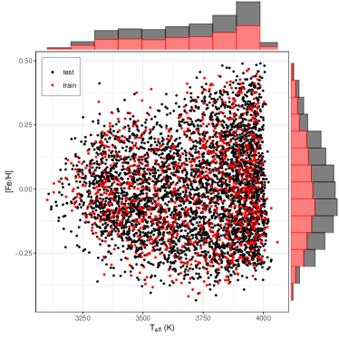
Figure 1: $T_{\text{eff}}$ vs. [Fe/H] diagram for the training (red) and test (black) subsamples from B20, showing the histograms for both variables.

Moreover, we tested the predictive performance of the calibrations with the sample presented by Montes et al. (2018), who studied 192 binary systems made of late F, G, or early K primaries and late K- or M-dwarf companion candidates. The authors carried out observations with the HERMES spectrograph at the 1.2 m Mercator telescope (Raskin et al., 2011) and obtained high-resolution spectra for the 192 primaries and five secondaries. These spectra were analyzed with the automatic code StePar (Tabernero et al., 2019), based on the equivalent width method, to derive precise stellar atmospheric parameters (effective temperature $T_{\rm eff}$, surface gravity $\log{g}$, and metallicity [Fe/H]). Since binaries are assumed to be born at the same time and from the same molecular cloud, the composition and age of the FGK-type primary star can be extrapolated to its secondary M dwarf (Desidera et al., 2006; Andrews et al., 2018). Next we checked our calibrations for these stars and compared them to other photometric estimations found in the literature.

2.2 Photometry and Data Filtering

Table 1: Data Filtering Criteria Applied to Astrophotometric Data

Survey	Filter
Gaia EDR3	parallax_over_error > 10
	ruwe < 1.4
	photo_g_mean_flux_over_error > 50
	photo_bp_mean_flux_over_error > 20
	photo_rp_mean_flux_over_error > 20
2MASS	Qfl = AAA
CatWISE2020	qph = AA**

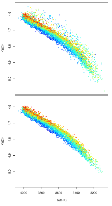
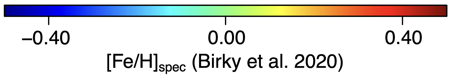
Figure 2: Kiel diagram of the B20 sample, before (upper panel) and after (lower panel) having removed the stars with lower surface gravity, i.e. not in the main sequence.

The third Gaia data release (Gaia DR3; Gaia Collaboration et al., 2022) provides the position and apparent magnitude in the $G$ band (330–1050 nm) for $1.8$ billion sources. For $1.5$ billion of them, parallax and proper motion data are also available. In addition, photometry in the $G_{\text{BP}}$ (330–680 nm) and $G_{\text{RP}}$ (630–1050 nm) bands is offered for another $1.5$ billion sources (Gaia Collaboration et al., 2016, 2021; Riello et al., 2021). To study M dwarfs, which have the peak of the emission beyond 1000 nm (Cifuentes et al., 2020), we also used information in the infrared (IR) wavelength range: 2MASS provides magnitudes in the near-IR $J$ ($1229$ nm), $H$ ($1639$ nm) and $K_{s}$ bands ($2152$ nm), while WISE offers data in the mid-IR bands $W1$, $W2$, $W3$, and $W4$, centered at 3316 nm, 4564 nm, 10 787 nm, and 21 915 nm, respectively. In particular, we used the data from the updated version CatWISE2020 (Marocco et al., 2021), which has enhanced sensitivity and accuracy. Initially, the analysis was performed with the AllWISE version (Cutri et al., 2021), but the uncertainties in the $W1-W2$ color index were a factor of $\sim 2$ larger than those of CatWISE2020.

First, we crossmatched the star samples described above with the Gaia DR3, 2MASS, and CatWISE2020 catalogs. For that, we used the Tool for OPerations on Catalogues And Tables (TOPCAT; Taylor 2005). In particular, we used the automatic positional crossmatch tool of the Centre de Données astronomiques de Strasbourg, CDS X-match, with a search radius of 5 arcsec and the “All” find option. Next, we used the Aladin sky atlas (Bonnarel et al., 2000) to inspect and correct the possibly mismatched cases.

These data do not have homogeneous quality. Consequently, we applied the data filtering indicated by Gaia Collaboration et al. (2018b). In particular, for color–magnitude diagrams, we made use of the absolute magnitude calculated using the Gaia parallax and selected only stars that fulfill the 10 % relative precision criterion, which corresponds to an uncertainty in $M_{G}$ lower than $0.22$ mag. Similarly, we applied filters to the relative flux error on the $G$, $G_{\text{BP}}$, and $G_{\text{RP}}$ magnitudes, which led to uncertainties of 0.022 mag, 0.054 mag, and 0.054 mag, respectively. To discard close unresolved or partially resolved binaries, we also applied a conservative filter in the astrometric quality indicator RUWE (renormalized unit weight error) as indicated by Lindegren et al. (2021), retaining those stars with RUWE values $<1.4$. For sources where the single-star model provides a good fit to the astrometric observations, the RUWE value is expected to be around $1.0$, and value significantly greater ($>1.4$) could indicate that the source is nonsingle or problematic for the astrometric solution.

In addition, we selected the stars with an “A” quality flag in the $J$, $H$, $K_{s}$, $W1$, and $W2$ bands, which corresponds to an approximate signal-to-noise ratio higher than 10. We discarded the $W3$ and $W4$ bands from our analysis, as they tend to present a lower photometric quality. All these criteria are compiled in Table 1. Applying these criteria to the 5875 stars presented by B20, we ended up with a sample of 5453 M dwarfs.

Finally, we removed young objects and/or evolved stars, i.e. stars arriving or leaving the main sequence, since for those cases the age plays an important role in the position of the star in the color–color and color–magnitude diagrams. To do this, we estimated the radii and masses of the stars with the $M_{K_{s}}$ absolute magnitude using the calibrations given by Mann et al. (2015) [Eq. 5] and Mann et al. (2019) [Eq. 5], respectively. With these two properties, we calculated the surface gravity $\log g$. The pre-main-sequence and the evolved stars are expected to have inflated radii, and thus lower surface gravities. Therefore, we calibrated the surface gravity using the effective temperature and metallicity and removed these lower surface gravity stars, those with a difference between the photometric and fitted surface gravities larger than $0.03$ dex. Hence we obtained a final sample of 4919 M dwarfs. We show in Fig. 2 the Kiel diagram ($T_{\text{eff}}$ vs. $\log g$) before and after having removed the lower $\log g$ stars. Note the gradient of metallicity present in the main sequence of the Kiel diagram, having decreasing $\log g$ with increasing metallicity for a given effective temperature.

The crossmatch between Montes et al. (2018), Gaia DR3, and CatWISE2020 catalogs resulted in a subsample of 115 M dwarfs among the 192 systems after having eliminated nonphysical pairs (Espada, 2019) or systems with double-lined spectroscopic binaries. Then, we applied the data filtering mentioned above and constrained to identical values as in B20, that is, early and mid M dwarfs between M0 V and M5 V, and having $1.85$ mag $\leq G-J\leq$ $3.10$ mag, $-0.10$ mag $\leq W1-W2\leq$ $0.24$ mag, and $-0.5\leq\text{[Fe/H]}\leq 0.5$ dex, and retrieved a final sample of 46 FGK+M systems to test the calibration.

2.3 Calibrations, Statistical Analysis, and Model Selection

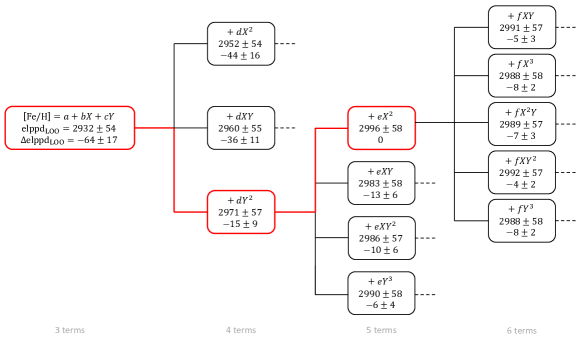
Figure 3: Comparison of different metallicity photometric calibrations with LOO-CV following a stepwise regression (forward selection) procedure, where $X=W1-W2$, $Y=G_{\text{BP}}-G_{\text{RP}}$, $\text{elppd}_{\text{LOO}}$ is the expected log-pointwise predictive density given by Eq. 1, and $\Delta\text{elppd}_{\text{LOO}}$ is the difference with respect to the model with the largest $\text{elppd}_{\text{LOO}}$, given by Eq. 2 and marked in red.

We divided the 4919 crossmatched, filtered M dwarfs from B20 into two subsamples: 1000 stars constitute the calibration or training sample, and the remaining 3919 stars are the test sample to check the accuracy of the calibrations. The $T_{\text{eff}}$–[Fe/H] space and their corresponding histograms for both subsamples are shown in Fig. 1.

The calibrations were derived with MCMC using Stan (Carpenter et al., 2017) through its R interface, namely RStan. Stan is a C++ library for Bayesian modeling and inference that incorporates, among other components, the Hamiltonian Monte Carlo no-U-turn sampler (HMC$+$NUTS) algorithm. After deriving different calibrations, we compared them with the LOO-CV criterion, which allowed us to choose the calibration that best reproduces the metallicity values by penalizing the more complicated models (i.e. with more free parameters) with respect to the simplest ones. The LOO-CV criterion defines the expected log-pointwise predictive density as:

$$\text{elppd}_{\text{LOO}}=\sum_{i=1}^{N}\log(P(x_{i}|\boldsymbol{x_{-i}}))$$ (1)

where $P(x_{i}|\boldsymbol{x_{-i}})$ denotes the probability of predicting $x_{i}$ using the data without the $i$th observation (Gelman et al., 2014; Vehtari et al., 2017). The value of $\text{elppd}_{\text{LOO}}$ can be either positive or negative since it uses the probability density, not the probability itself. The model with the largest $\text{elppd}_{\text{LOO}}$ presents the best predictive accuracy. The computed $\text{elppd}_{\text{LOO}}$ is defined as the sum of $N$ independent components, so its standard error can be computed as the standard deviation of the $N$ components divided by $\sqrt{N}$. We used the R package loo for implementing the necessary functions and for estimating $\text{elppd}_{\text{LOO}}$ with the Pareto smoothed importance sampling method (Vehtari et al., 2015).

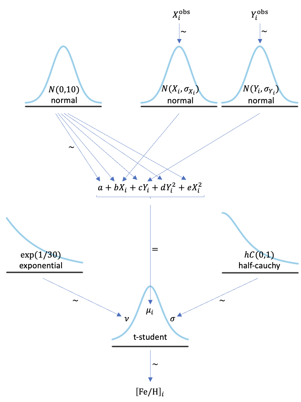
Figure 4: Summary of the distributions used in the Stan model for the robust regression, where $X_{i}^{\rm obs}$ and $Y_{i}^{\rm obs}$ indicate the observed values of the predictors, with their observational errors $\sigma_{X_{i}}$ and $\sigma_{Y_{i}}$, respectively. Therefore the observed values of the predictors come from a normal distribution (with standard deviations equal to the observed errors) around the ‘true’ values $X_{i}$ and $Y_{i}$. In the same way, $\mu$ is the predicted value of the metallicity, which relates to the observed metallicity through a $t$-distribution with parameters $\nu$ (degrees of freedom) and $\sigma$ (scale parameter). For the coefficients we assumed normal priors, while an exponential distribution and a half-Cauchy distribution are used as priors for $\nu$ and $\sigma$, respectively. See Kruschke (2014) for more details on the interpretation of this kind of graph.

In order to derive the best calibration using the LOO-CV criterion, we tried different calibrations, starting with a linear model and increasingly adding more terms following a stepwise regression procedure (forward selection), shown in Fig. 3 for the $W1-W2$ vs. $G_{\text{BP}}-G_{\text{RP}}$ diagram as an example. For this case, we performed the stepwise regression including up to six terms and found that the model with the best predictive performance (i.e., the largest $\text{elppd}_{\text{LOO-CV}}$) is given by:

$$\text{[Fe/H]}=a+bX+cY+dY^{2}+eX^{2}$$ (2)

The distribution of the residuals of the calibrations exhibited extended wings and could not be fitted by a Gaussian distribution. As a result, we used a generalized linear model with a $t$-distribution instead of a Gaussian one to model the corresponding likelihood. Furthermore, this robust regression (with $t$-distribution instead of the Gaussian likelihood) significantly increased the $\text{elppd}_{\text{LOO-CV}}$. For the robust regression, we used weakly informative priors for the coefficients, that is, $a,b,c,d,e\sim$ normal(0,10). The likelihood is given by $\text{[Fe/H]}\sim$ t-Student$(\mu,\nu,\sigma)$, where $\mu$ is the expression in Eq. 2, and the priors for the scale parameter and degrees of freedom are $\sigma\sim$ half-Cauchy(0,1) and $\nu\sim$ exponential(1/30), respectively. These are suitable priors for $\sigma$ and $\nu$ since the half-Cauchy distribution is a less informative prior than the normal distribution, with heavier tails, and the exponential(1/30) distribution captures the behavior of the degrees of freedom in the $t$-distribution, that is, nearly all the variation in the family of $t$-distribution happens when $\nu$ is fairly small and for $\nu>30$ the $t$-distribution is essentially normal. Therefore, since $\nu=30$ is the mean of the exponential(1/30) distribution, with this prior we give the same weights to the low and high regimes of $\nu$. We provide a graphical representation of the model in Fig. 4 (see Kruschke 2014).

Table 2: Fit Parameters of Color–Color Diagram Calibrations

$X$	$Y$	$a$	$b$	$c$	$d$	$e$	$\sigma$	$\nu$	$\text{elppd}_{\text{LOO}}$	$\Delta\text{elppd}_{\text{LOO}}$
(mag)	(mag)	(dex)	(mag-1)	(mag-1)	(mag-2)	(mag-2)	(dex)
$W1-W2$	$G_{\text{BP}}-G_{\text{RP}}$	$-2.72\pm 0.18$	$-3.96\pm 0.13$	$1.91\pm 0.16$	$-0.253\pm 0.036$	$0.65\pm 0.90$	$0.0960\pm 0.0049$	$22.32\pm 19.58$	$2996\pm 58$	$0$
$W1-W2$	$G-H$	$-4.92\pm 0.47$	$-3.54\pm 0.11$	$2.49\pm 0.30$	$-0.266\pm 0.049$	$2.07\pm 0.79$	$0.0875\pm 0.0050$	$8.27\pm 4.13$	$2974\pm 61$	$-21\pm 26$
$W1-W2$	$G-K_{s}$	$-4.39\pm 0.43$	$-3.71\pm 0.12$	$2.03\pm 0.26$	$-0.189\pm 0.040$	$2.45\pm 0.80$	$0.0875\pm 0.0048$	$8.62\pm 4.81$	$2965\pm 62$	$-31\pm 25$
$W1-W2$	$G-J$	$-3.32\pm 0.29$	$-3.87\pm 0.13$	$2.06\pm 0.24$	$-0.243\pm 0.049$	$1.11\pm 0.88$	$0.0953\pm 0.0052$	$15.77\pm 13.79$	$2891\pm 59$	$-105\pm 20$
$W1-W2$	$G_{\text{RP}}-K_{s}$	$-4.93\pm 0.43$	$-3.52\pm 0.12$	$3.50\pm 0.38$	$-0.536\pm 0.085$	$3.05\pm 0.79$	$0.0863\pm 0.0048$	$7.19\pm 2.81$	$2882\pm 64$	$-113\pm 33$
$W1-W2$	$G_{\text{RP}}-H$	$-5.70\pm 0.49$	$-3.20\pm 0.11$	$4.60\pm 0.48$	$-0.83\pm 0.12$	$2.34\pm 0.80$	$0.0878\pm 0.0049$	$7.35\pm 2.80$	$2873\pm 62$	$-123\pm 36$
$W1-W2$	$G_{\text{RP}}-J$	$-2.87\pm 0.22$	$-3.70\pm 0.13$	$3.23\pm 0.32$	$-0.70\pm 0.11$	$1.21\pm 0.90$	$0.0995\pm 0.0052$	$19.36\pm 17.28$	$2765\pm 59$	$-231\pm 29$
$W1-W2$	$G-W1$	$-3.59\pm 0.44$	$-3.43\pm 0.14$	$1.56\pm 0.26$	$-0.131\pm 0.037$	$2.06\pm 0.87$	$0.1024\pm 0.0055$	$13.12\pm 10.73$	$2720\pm 58$	$-276\pm 18$
$W1-W2$	$G-W2$	$-3.14\pm 0.37$	$-4.14\pm 0.16$	$1.28\pm 0.21$	$-0.089\pm 0.030$	$2.52\pm 0.93$	$0.1001\pm 0.0059$	$13.44\pm 11.48$	$2696\pm 60$	$-300\pm 19$
$W1-W2$	$G_{\text{RP}}-W1$	$-3.72\pm 0.43$	$-3.20\pm 0.14$	$2.44\pm 0.36$	$-0.327\pm 0.076$	$2.46\pm 0.91$	$0.1061\pm 0.0056$	$11.97\pm 8.70$	$2603\pm 57$	$-393\pm 23$
$W1-W2$	$G_{\text{RP}}-W2$	$-3.00\pm 0.35$	$-4.15\pm 0.17$	$1.80\pm 0.29$	$-0.188\pm 0.059$	$3.16\pm 0.96$	$0.1036\pm 0.0060$	$12.48\pm 10.09$	$2568\pm 59$	$-428\pm 24$

A Bayesian approach to error measurement can be formulated by treating the true quantities being measured as missing data or latent variables, needing a model of how the measurements are derived from the true values. We can suppose that the ‘true’ values of a predictor $A_{i}$, for example the magnitude in a given photometric band, are not known, but for each $i$ star, a measurement $A_{i}^{\rm obs}$ of $A_{i}$ is available. Then the approach is to assume that the measured values arise from a normal distribution with a mean equal to the true value and some measurement error $\sigma_{A_{i}}$, that is, $A_{i}^{\rm obs}\sim normal(A_{i},\sigma_{A_{i}})$. Therefore, the regression is not performed with the measured values $A_{i}^{\rm obs}$ but with the true ones $A_{i}$ (see Fig. 4).

Finally, to ensure the convergence of the MCMC chains we applied the Gelman–Rubin diagnostic or shrink factor $\hat{R}$ (Gelman & Rubin, 1992; Brooks & Gelman, 1998), which analyzes the difference between multiple Markov chains. The convergence is assessed by comparing the estimated between-chains and within-chain variances for each model parameter. If $\hat{R}<1.1$ for all parameters, one can be confident that convergence has been reached. In our case, we obtained a shrink factor of $\hat{R}=1.0$ for all parameters. We typically run three simultaneous chains with 3000 steps in each of them and 500 warm-up iterations.

3 Results and discussion

3.1 Color–Color Diagrams

Color–color diagrams allow us to compare apparent magnitudes at different wavelengths. In these diagrams the chemical composition plays a fundamental role, showing a gradient of metallicity that is more noticeable for cool stars (Gaia Collaboration et al., 2018b). In particular, the $W1-W2$ color index constitutes an appropriate metallicity indicator (Schmidt et al., 2016).

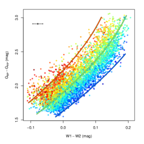
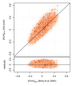
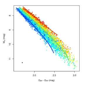
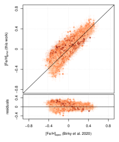
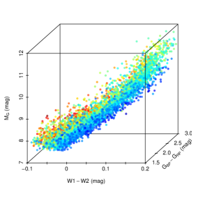
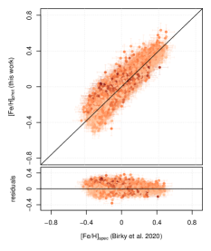
Figure 5: Left panels: from top to bottom, representative examples of color–color, color–magnitude, and color–color–magnitude diagrams of the stars from B20, color-coded by [Fe/H]${}_{\text{spec}}$, with the respective calibrations given by this work (red: $\text{[Fe/H]}=0.3$ dex, green: $\text{[Fe/H]}=0.0$ dex, blue: $\text{[Fe/H]}=-0.3$ dex). The mean uncertainties of the color indices and absolute magnitudes involved are also shown with a black dot. Right panels: comparison between the spectroscopic metallicity values reported by B20 and the photometric estimations with the corresponding diagrams in the left for the 3919 stars from the test subsample, and respective residuals, color-coded by $G_{\text{BP}}-G_{\text{RP}}$ color index (darker symbols: cooler stars; lighter symbols: warmer stars). The solid lines denote the 1:1 relationship and the residuals $=0$.

In Table 2 we present the posterior mean and standard deviation of the coefficients of the calibration given by Eq. 2 for different color–color combinations, the scale parameter and degrees of freedom of the Student’s $t$-distribution, and their comparison with LOO-CV, sorted from the best to the worst combination according to their elppd value. The posterior distributions of the coefficients are Gaussian. All these calibrations fit the observed metallicities with a residual standard deviation of $0.08$–$0.09$ dex, of the same order as the [Fe/H] uncertainty provided by B20, which means we are performing our regression until the observational limit. An example of color–color diagram is shown in the top left panel of Fig. 5. The remaining color–color diagram combinations are available in Fig. A.1.

In the top right panels of Fig. 5 we also represent the [Fe/H] values reported by B20 versus the estimated values using the $W1-W2$ vs. $G_{\text{BP}}-G_{\text{RP}}$ color–color diagram, and the corresponding residuals, for the 3919 stars from the test subsample, color-coded by $G_{\text{BP}}-G_{\text{RP}}$ color index. We conclude that most of the estimated metallicities follow the one-to-one relationship and that there is no correlation between them and $T_{\rm eff}$, as expected. Some photometric metallicities are more than $2\sigma$ above or below the spectroscopic value given by B20, but they are just 112 stars, $2.9\,\%$ of the test sample.

3.2 Color–Magnitude Diagrams

Color–magnitude or Hertzsprung–Russell diagrams represent the absolute magnitude or luminosity versus the color index, spectral type, or $T_{\rm eff}$. The position of a star in these diagrams is mainly given by its initial mass, chemical composition, and age, but other effects such as rotation, stellar winds, or magnetic fields also play a role (Gaia Collaboration et al., 2018b). Similar to what is observed in our color–color diagrams, color–magnitude diagrams also present a metallicity gradient.

We proceeded with the analysis as in the previous section. In Table 3 we present the coefficients of the calibration given by Eq. 2 for different color–magnitude combinations and their comparison using the LOO-CV criterion.

In the central panels of Fig. 5, we represent the color–magnitude diagram $G_{\text{BP}}-G_{\text{RP}}$ vs. $M_{G}$ of the 4919 stars from B20 (left) and the comparison between the spectroscopic [Fe/H] values and the corresponding estimated values for the 3 919 stars from the test subsample (right). Again, the rest of color–magnitude diagrams can be found in Figs. A.2, A.3, A.4, and A.5. In the case of the $G_{\text{BP}}-G_{\text{RP}}$ vs. $M_{G}$ color–magnitude diagram, 237 stars ($6.0\,\%$) are more than $2\sigma$ above or below the spectroscopic value.

Table 3: Fit Parameters of Color–Magnitude Diagram Calibrations

$X$	$Y$	$a$	$b$	$c$	$d$	$e$	$\sigma$	$\nu$	$\text{elppd}_{\text{LOO}}$	$\Delta\text{elppd}_{\text{LOO}}$
(mag)	(mag)	(dex)	(mag-1)	(mag-1)	(mag-2)	(mag-2)	(dex)
$G_{\text{BP}}-G_{\text{RP}}$	$M_{G}$	$8.89\pm 0.36$	$5.89\pm 0.24$	$-3.22\pm 0.13$	$0.1432\pm 0.0068$	$-0.933\pm 0.054$	$0.0706\pm 0.0033$	$4.20\pm 0.71$	$3611\pm 61$	$0$
$G_{\text{BP}}-G_{\text{RP}}$	$M_{K_{s}}$	$4.75\pm 0.22$	$2.93\pm 0.16$	$-2.63\pm 0.11$	$0.1790\pm 0.0090$	$-0.416\pm 0.036$	$0.0718\pm 0.0034$	$4.43\pm 0.79$	$3519\pm 62$	$-92\pm 24$
$G_{\text{BP}}-G_{\text{RP}}$	$M_{H}$	$4.44\pm 0.22$	$3.19\pm 0.17$	$-2.54\pm 0.10$	$0.1660\pm 0.0083$	$-0.468\pm 0.037$	$0.0710\pm 0.0035$	$4.08\pm 0.70$	$3491\pm 62$	$-120\pm 22$
$G_{\text{BP}}-G_{\text{RP}}$	$M_{J}$	$7.34\pm 0.31$	$3.49\pm 0.17$	$-3.19\pm 0.13$	$0.1953\pm 0.0094$	$-0.525\pm 0.039$	$0.0725\pm 0.0035$	$4.25\pm 0.75$	$3460\pm 62$	$-151\pm 18$
$G-W1$	$M_{K_{s}}$	$2.25\pm 0.32$	$2.39\pm 0.23$	$-2.29\pm 0.10$	$0.1559\pm 0.0084$	$-0.209\pm 0.034$	$0.0761\pm 0.0034$	$4.32\pm 0.70$	$3399\pm 63$	$-212\pm 50$
$G-W1$	$M_{H}$	$1.63\pm 0.32$	$2.70\pm 0.24$	$-2.19\pm 0.10$	$0.1430\pm 0.0081$	$-0.250\pm 0.036$	$0.0766\pm 0.0035$	$4.25\pm 0.68$	$3372\pm 63$	$-239\pm 49$
$G-W1$	$M_{J}$	$3.91\pm 0.34$	$2.94\pm 0.25$	$-2.72\pm 0.12$	$0.1665\pm 0.0089$	$-0.279\pm 0.037$	$0.0773\pm 0.0035$	$4.38\pm 0.74$	$3367\pm 62$	$-244\pm 47$
$G-K_{s}$	$M_{H}$	$1.16\pm 0.35$	$2.84\pm 0.27$	$-2.072\pm 0.098$	$0.1356\pm 0.0079$	$-0.276\pm 0.041$	$0.0773\pm 0.0037$	$4.66\pm 0.85$	$3351\pm 63$	$-260\pm 46$
$G-K_{s}$	$M_{J}$	$3.24\pm 0.38$	$3.05\pm 0.28$	$-2.55\pm 0.12$	$0.1556\pm 0.0089$	$-0.303\pm 0.043$	$0.0797\pm 0.0038$	$5.26\pm 1.11$	$3323\pm 62$	$-288\pm 44$
$G-H$	$M_{K_{s}}$	$0.65\pm 0.40$	$3.09\pm 0.30$	$-2.009\pm 0.099$	$0.1366\pm 0.0082$	$-0.331\pm 0.049$	$0.0768\pm 0.0038$	$4.30\pm 0.78$	$3311\pm 63$	$-300\pm 45$
$G-W1$	$M_{G}$	$2.64\pm 0.34$	$4.73\pm 0.34$	$-2.42\pm 0.12$	$0.1064\pm 0.0063$	$-0.486\pm 0.049$	$0.0807\pm 0.0035$	$4.57\pm 0.74$	$3270\pm 61$	$-341\pm 52$
$G-K_{s}$	$M_{K_{s}}$	$1.80\pm 0.37$	$2.39\pm 0.27$	$-2.10\pm 0.10$	$0.1427\pm 0.0087$	$-0.215\pm 0.042$	$0.0817\pm 0.0038$	$5.39\pm 1.14$	$3268\pm 62$	$-343\pm 48$
$G-K_{s}$	$M_{G}$	$1.69\pm 0.37$	$4.93\pm 0.36$	$-2.24\pm 0.11$	$0.0984\pm 0.0059$	$-0.530\pm 0.054$	$0.0796\pm 0.0039$	$5.38\pm 1.20$	$3256\pm 63$	$-355\pm 48$
$G-H$	$M_{J}$	$1.89\pm 0.41$	$3.66\pm 0.31$	$-2.35\pm 0.12$	$0.1431\pm 0.0086$	$-0.413\pm 0.051$	$0.0785\pm 0.0040$	$4.43\pm 0.86$	$3252\pm 63$	$-360\pm 42$
$G-J$	$M_{K_{s}}$	$3.42\pm 0.27$	$2.84\pm 0.25$	$-2.36\pm 0.11$	$0.1600\pm 0.0092$	$-0.351\pm 0.052$	$0.0825\pm 0.0041$	$5.33\pm 1.22$	$3245\pm 62$	$-366\pm 40$
$G-W2$	$M_{K_{s}}$	$4.43\pm 0.29$	$1.95\pm 0.21$	$-2.72\pm 0.12$	$0.185\pm 0.010$	$-0.143\pm 0.031$	$0.0797\pm 0.0037$	$4.20\pm 0.69$	$3241\pm 63$	$-370\pm 46$
$G_{\text{RP}}-W1$	$M_{K_{s}}$	$1.49\pm 0.33$	$3.82\pm 0.33$	$-2.16\pm 0.10$	$0.1481\pm 0.0085$	$-0.531\pm 0.070$	$0.0785\pm 0.0034$	$4.19\pm 0.63$	$3223\pm 64$	$-388\pm 59$
$G-W2$	$M_{H}$	$3.86\pm 0.28$	$2.30\pm 0.22$	$-2.65\pm 0.12$	$0.1733\pm 0.0095$	$-0.189\pm 0.032$	$0.0794\pm 0.0037$	$3.93\pm 0.61$	$3205\pm 63$	$-406\pm 45$
$G-J$	$M_{H}$	$2.97\pm 0.26$	$3.18\pm 0.25$	$-2.27\pm 0.11$	$0.1481\pm 0.0087$	$-0.414\pm 0.052$	$0.0821\pm 0.0042$	$4.91\pm 1.08$	$3203\pm 62$	$-408\pm 39$
$G_{\text{RP}}-W1$	$M_{H}$	$0.91\pm 0.32$	$4.20\pm 0.34$	$-2.057\pm 0.099$	$0.1352\pm 0.0080$	$-0.607\pm 0.071$	$0.0792\pm 0.0035$	$4.15\pm 0.63$	$3193\pm 64$	$-418\pm 58$
$G_{\text{RP}}-W1$	$M_{J}$	$3.04\pm 0.36$	$4.51\pm 0.36$	$-2.55\pm 0.12$	$0.1566\pm 0.0089$	$-0.661\pm 0.077$	$0.0797\pm 0.0035$	$4.25\pm 0.65$	$3186\pm 63$	$-426\pm 56$
$G-H$	$M_{H}$	$0.13\pm 0.40$	$3.26\pm 0.31$	$-1.862\pm 0.095$	$0.1212\pm 0.0077$	$-0.358\pm 0.051$	$0.0804\pm 0.0040$	$4.45\pm 0.83$	$3167\pm 62$	$-445\pm 46$
$G-W2$	$M_{J}$	$6.75\pm 0.35$	$2.57\pm 0.23$	$-3.32\pm 0.15$	$0.203\pm 0.011$	$-0.221\pm 0.034$	$0.0816\pm 0.0039$	$4.17\pm 0.71$	$3158\pm 62$	$-453\pm 42$
$G-H$	$M_{G}$	$-0.02\pm 0.41$	$5.52\pm 0.40$	$-1.97\pm 0.10$	$0.0857\pm 0.0055$	$-0.656\pm 0.064$	$0.0788\pm 0.0042$	$4.45\pm 0.87$	$3154\pm 63$	$-457\pm 46$
$G_{\text{RP}}-K_{s}$	$M_{H}$	$0.16\pm 0.38$	$4.53\pm 0.41$	$-1.873\pm 0.097$	$0.1228\pm 0.0078$	$-0.699\pm 0.090$	$0.0785\pm 0.0039$	$4.49\pm 0.80$	$3137\pm 65$	$-474\pm 54$
$G_{\text{RP}}-K_{s}$	$M_{J}$	$2.00\pm 0.40$	$4.80\pm 0.42$	$-2.29\pm 0.12$	$0.1398\pm 0.0087$	$-0.749\pm 0.094$	$0.0810\pm 0.0040$	$5.07\pm 1.06$	$3104\pm 64$	$-507\pm 53$
$G_{\text{RP}}-K_{s}$	$M_{K_{s}}$	$0.79\pm 0.39$	$3.87\pm 0.40$	$-1.89\pm 0.10$	$0.1289\pm 0.0086$	$-0.568\pm 0.090$	$0.0834\pm 0.0039$	$5.11\pm 0.99$	$3055\pm 63$	$-556\pm 56$
$G_{\text{RP}}-W2$	$M_{K_{s}}$	$4.68\pm 0.28$	$2.80\pm 0.29$	$-2.77\pm 0.13$	$0.189\pm 0.011$	$-0.306\pm 0.060$	$0.0824\pm 0.0037$	$3.99\pm 0.60$	$3047\pm 64$	$-564\pm 53$
$G_{\text{RP}}-H$	$M_{K_{s}}$	$-0.86\pm 0.43$	$5.28\pm 0.47$	$-1.705\pm 0.096$	$0.1156\pm 0.0080$	$-0.94\pm 0.12$	$0.0793\pm 0.0041$	$4.23\pm 0.77$	$3046\pm 64$	$-565\pm 53$
$G-J$	$M_{J}$	$5.22\pm 0.33$	$3.27\pm 0.27$	$-2.70\pm 0.13$	$0.1646\pm 0.0099$	$-0.433\pm 0.056$	$0.0905\pm 0.0045$	$6.29\pm 1.83$	$3035\pm 60$	$-576\pm 40$
$G-J$	$M_{G}$	$5.12\pm 0.33$	$5.59\pm 0.37$	$-2.57\pm 0.13$	$0.1131\pm 0.0069$	$-0.797\pm 0.074$	$0.0879\pm 0.0047$	$6.03\pm 2.06$	$3024\pm 61$	$-587\pm 40$
$G-W2$	$M_{G}$	$6.96\pm 0.37$	$4.76\pm 0.34$	$-3.32\pm 0.16$	$0.1469\pm 0.0084$	$-0.457\pm 0.049$	$0.0859\pm 0.0039$	$4.10\pm 0.64$	$3012\pm 60$	$-599\pm 46$
$G_{\text{RP}}-W2$	$M_{H}$	$4.16\pm 0.28$	$3.27\pm 0.30$	$-2.70\pm 0.13$	$0.177\pm 0.010$	$-0.395\pm 0.061$	$0.0825\pm 0.0039$	$3.80\pm 0.57$	$3005\pm 64$	$-606\pm 52$
$G_{\text{RP}}-W1$	$M_{G}$	$1.49\pm 0.34$	$6.74\pm 0.46$	$-2.13\pm 0.11$	$0.0939\pm 0.0061$	$-1.042\pm 0.096$	$0.0845\pm 0.0036$	$4.24\pm 0.63$	$2985\pm 62$	$-626\pm 63$
$G_{\text{RP}}-H$	$M_{J}$	$0.13\pm 0.45$	$5.92\pm 0.50$	$-1.94\pm 0.11$	$0.1177\pm 0.0082$	$-1.08\pm 0.12$	$0.0815\pm 0.0044$	$4.44\pm 0.87$	$2977\pm 64$	$-634\pm 51$
$G_{\text{RP}}-W2$	$M_{J}$	$7.13\pm 0.35$	$3.59\pm 0.32$	$-3.37\pm 0.16$	$0.207\pm 0.012$	$-0.448\pm 0.066$	$0.0850\pm 0.0040$	$4.04\pm 0.65$	$2947\pm 63$	$-664\pm 49$
$G_{\text{RP}}-J$	$M_{K_{s}}$	$3.58\pm 0.26$	$4.23\pm 0.35$	$-2.17\pm 0.12$	$0.1468\pm 0.0097$	$-0.94\pm 0.13$	$0.0895\pm 0.0046$	$6.22\pm 1.81$	$2935\pm 62$	$-676\pm 47$
$G_{\text{RP}}-K_{s}$	$M_{G}$	$0.15\pm 0.39$	$7.11\pm 0.51$	$-1.87\pm 0.11$	$0.0816\pm 0.0056$	$-1.17\pm 0.11$	$0.0806\pm 0.0042$	$4.78\pm 0.95$	$2917\pm 65$	$-695\pm 59$
$G_{\text{RP}}-H$	$M_{H}$	$-1.25\pm 0.45$	$5.36\pm 0.50$	$-1.547\pm 0.095$	$0.1001\pm 0.0077$	$-0.96\pm 0.12$	$0.0841\pm 0.0044$	$4.53\pm 0.89$	$2901\pm 63$	$-710\pm 54$
$G_{\text{RP}}-J$	$M_{H}$	$3.23\pm 0.26$	$4.57\pm 0.37$	$-2.06\pm 0.11$	$0.1338\pm 0.0091$	$-1.05\pm 0.13$	$0.0903\pm 0.0048$	$6.02\pm 1.78$	$2884\pm 62$	$-727\pm 47$
$G_{\text{RP}}-H$	$M_{G}$	$-1.98\pm 0.46$	$8.06\pm 0.62$	$-1.467\pm 0.096$	$0.0628\pm 0.0051$	$-1.51\pm 0.15$	$0.0828\pm 0.0047$	$4.40\pm 0.88$	$2778\pm 65$	$-833\pm 56$
$G_{\text{RP}}-J$	$M_{J}$	$5.20\pm 0.36$	$4.48\pm 0.40$	$-2.38\pm 0.14$	$0.144\pm 0.011$	$-1.03\pm 0.14$	$0.1007\pm 0.0051$	$8.68\pm 4.77$	$2701\pm 59$	$-910\pm 47$
$G_{\text{RP}}-W2$	$M_{G}$	$7.32\pm 0.41$	$6.36\pm 0.49$	$-3.24\pm 0.18$	$0.1430\pm 0.0093$	$-0.877\pm 0.098$	$0.0928\pm 0.0041$	$3.94\pm 0.57$	$2643\pm 61$	$-968\pm 56$
$G_{\text{RP}}-J$	$M_{G}$	$5.03\pm 0.39$	$7.00\pm 0.54$	$-2.08\pm 0.14$	$0.0897\pm 0.0074$	$-1.70\pm 0.19$	$0.1019\pm 0.0058$	$9.45\pm 6.34$	$2530\pm 60$	$-1082\pm 50$

Table 4: Fit Parameters of Color–Color–Magnitude Diagram Calibrations

$Z$	$a$	$b$	$c$	$d$	$e$	$f$	$\sigma$	$\nu$	$\text{elppd}_{\text{LOO-CV}}$	$\Delta\text{elppd}_{\text{LOO-CV}}$
(mag)	(dex)	(mag-1)	(mag-1)	(mag-1)	(mag-2)	(mag-2)	(dex)
$M_{G}$	$5.87\pm 0.44$	$-1.40\pm 0.12$	$5.08\pm 0.24$	$-2.45\pm 0.14$	$-0.788\pm 0.052$	$0.1094\pm 0.0071$	$0.0691\pm 0.0032$	$5.43\pm 1.19$	$3961\pm 59$	$0$
$M_{K_{s}}$	$2.70\pm 0.27$	$-1.39\pm 0.12$	$2.82\pm 0.15$	$-1.99\pm 0.11$	$-0.392\pm 0.034$	$0.1355\pm 0.0090$	$0.0677\pm 0.0032$	$4.82\pm 0.93$	$3864\pm 61$	$-97\pm 20$
$M_{J}$	$4.42\pm 0.37$	$-1.54\pm 0.12$	$3.23\pm 0.17$	$-2.34\pm 0.14$	$-0.472\pm 0.037$	$0.1442\pm 0.0097$	$0.0697\pm 0.0034$	$5.37\pm 1.19$	$3859\pm 60$	$-102\pm 15$
$M_{H}$	$2.42\pm 0.27$	$-1.42\pm 0.13$	$3.01\pm 0.16$	$-1.90\pm 0.11$	$-0.430\pm 0.036$	$0.1248\pm 0.0087$	$0.0686\pm 0.0033$	$4.86\pm 0.95$	$3839\pm 60$	$-121\pm 18$

3.3 Color–Color–Magnitude Diagrams

Some authors, such as Davenport & Dorn-Wallenstein (2019), added an absolute magnitude as a third variable in their calibrations in order to improve their estimations, which we refer to as color–color–magnitude diagrams. Thus, we performed a stepwise regression using three variables, finding that the model with the best predictive performance is given by:

$$\text{[Fe/H]}=a+bX+cY+dZ+eY^{2}+fZ^{2},$$ (3)

where, as an example, $X=W1-W2$ and $Y=G_{\text{BP}}-G_{\text{RP}}$ are two color indices, and the absolute magnitude $Z=M_{G}$ is added as a third variable. We display the coefficients of the calibration given by Eq. 3 in Table 4. As Davenport & Dorn-Wallenstein (2019), we found an improvement by adding $M_{G}$ to the $W1-W2$ vs. $G_{\text{BP}}-G_{\text{RP}}$ diagram, having that the residual dispersion $\sigma$ and the $\text{elppd}_{\text{LOO}}$ improve with the addition of this third independent variable. The three-dimensional color–color–magnitude $W1-W2$ vs. $G_{\text{BP}}-G_{\text{RP}}$ vs. $M_{G}$ and the comparison between the spectroscopic and estimated [Fe/H] values for the 3919 test stars are plotted in Fig. 5 (bottom panels) and the pairs plot of the coefficients regarding this model is shown in Fig. A.6. For this color–color–magnitude diagram, 201 stars ($5.1\,\%$) are more than $2\sigma$ above or below the spectroscopic value. The statistics of the residuals regarding the three calibrations displayed in Fig. 5 are shown in Table 5.

Table 5: Statistics of the Residuals of the Best Color–Color, Color–Magnitude, and Color–Color–Magnitude calibrations

	$\overline{x}$	$\tilde{x}$	$\sigma_{x}$	MAD($x$)
$W1-W2$ vs. $G_{\text{BP}}-G_{\text{RP}}$	$0.003$	$-0.004$	$0.112$	$0.103$
$G_{\text{BP}}-G_{\text{RP}}$ vs. $M_{G}$	$0.012$	$-0.006$	$0.095$	$0.072$
$W1-W2$ vs. $G_{\text{BP}}-G_{\text{RP}}$ vs. $M_{G}$	$0.009$	$-0.006$	$0.089$	$0.075$

Table 6: Statistics of the Differences between Primary’s [Fe/H]${}_{\text{spec}}$ and Secondary’s [Fe/H]${}_{\text{phot}}$

	$\overline{x}$	$\tilde{x}$	$\sigma_{x}$	MAD($x$)	$r$	$r_{\rm S}$
B05	$0.144$	$0.111$	$0.147$	$0.105$	$0.707$	$0.671$
JA09	$-0.064$	$-0.086$	$0.206$	$0.144$	$0.688$	$0.656$
N12	$0.071$	$0.039$	$0.149$	$0.115$	$0.693$	$0.659$
M13	$0.043$	$0.063$	$0.144$	$0.156$	$0.649$	$0.641$
DD19	$0.047$	$0.056$	$0.176$	$0.167$	$0.528$	$0.518$
R21	$-0.007$	$0.001$	$0.105$	$0.089$	$0.842$	$0.783$
This work	$-0.012$	$-0.004$	$0.087$	$0.081$	$0.897$	$0.827$

3.4 Comparison with Previous Photometric Estimations

We compared our results with previous photometric estimations from the literature (B05: Bonfils et al. 2005 [Eq. 1], JA09: Johnson & Apps 2009 [Eq. 1], N12: Neves et al. 2012 [Eq. 3], M13: Mann et al. 2013 [Eq. 29], DD19: Davenport & Dorn-Wallenstein 2019 [ingot], R21: Rains et al. 2021 [Eq. 2]). To do this, we used the stellar sample of FGK+M binary systems presented by Montes et al. (2018). We did not compare with Schlaufman & Laughlin (2010) and Johnson et al. (2012) because updated versions of their calibrations are in N12 and M13, respectively. We did not compare either with Schmidt et al. (2016), Hejazi et al. (2015) and Medan et al. (2021) since less than the $50\,\%$ of the M-dwarf companions presented in Montes et al. (2018) have a counterpart in the SDSS catalog, nor with Dittmann et al. (2016) which requires the MEarth photometry. In Fig. 6 we represent the spectroscopic metallicity values of the primary stars reported by Montes et al. (2018) versus the photometrically estimated values for the M-dwarf companions. In our case, we use the best accurate color–color–magnitude calibration. The open circles represent the 115 stars and the filled circles the 46 stars that remain after applying the criteria described in Sect. 2 (i.e. stars with good photometric and astrometric data). Qualitatively, our estimations and the ones from R21 for the 46 stars follow the 1:1 relationship with less dispersion than the estimated values from previous studies. In Fig. A.7 we compared all the photometric estimations for the metallicity of M-dwarf companions. We found that the calibrations by B05, JA09 and N12 are highly correlated, since they are based on the same color–magnitude diagram. We also noted that our estimations show a good consistency with the ones by R21.

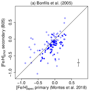
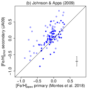
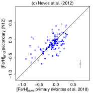
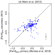
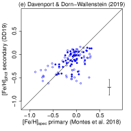
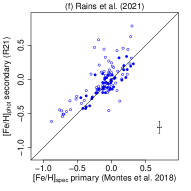
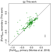
Figure 6: Comparison between the spectroscopic metallicity of the the FGK-type primary stars measured by Montes et al. (2018) and the photometric metallicity estimated by B05, JA09, N12, M13, DD19, R21 (blue), and by us (green) using the best accurate color–color–magnitude calibration from Table 4 of the 46 secondary M dwarfs of Sect. 2. The open circles represent the 115 stars and the filled circles the 46 stars with good photometric and astrometric data. The solid line denotes the 1:1 relationship. The error bars show the mean spectroscopic uncertainty and the MAD of the differences between the metallicities of each of the literature methods and the spectroscopic values.

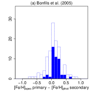
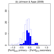
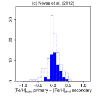
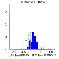
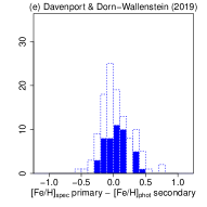
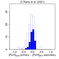
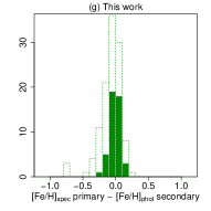
Figure 7: Same as Fig. 6 but for the distributions of the difference between primary’s [Fe/H]${}_{\text{spec}}$ and solid and dashed histograms instead of solid and open circles.

For a more quantitative comparison, we studied the distributions of the differences between the primary’s [Fe/H]${}_{\text{spec}}$ and the secondary’s [Fe/H]${}_{\text{phot}}$. The histograms of these distributions are plotted in Fig. 7, while some statistics are compiled in Table 6, along with the Pearson’s and Spearman’s correlation coefficients for the spectroscopic and photometric metallicity values. Our metallicity estimations and their uncertainties, shown for the 46 M dwarfs in Table B.1, are quantitatively less biased and have less dispersion and a greater correlation than those from previous studies. Our calibration can also be used even when some of the filtering criteria are not met, obtaining a distribution that, despite having outliers, is not biased and reproduces reasonably well the metallicity values.

4 Summary

In the present work we studied the photometric estimations of metallicity for M dwarfs. The precision, accuracy, and homogeneity of both astrometry and photometry from Gaia DR3, complemented by near- and mid-IR photometry from 2MASS and CatWISE2020, allowed us to study different calibrations based on color–color and color–magnitude diagrams. In order to obtain the best quality for calibrations, we filtered our data and removed multiple stars, lower surface gravity stars or with low photometric or astrometric quality.

Using the sample presented by B20, we derived several photometric calibrations using MCMC methods with Stan. We studied the metallicity gradient shown in color–color and color–magnitude diagrams in order to estimate the metallicity of early and mid M dwarfs (down to M5.0 V). We compared the predictive performance of the different calibrations with the LOO-CV criterion, and combined the information in a three-dimensional color–color–magnitude diagram. We obtained an improvement when adding an absolute magnitude as a third variable to the optical-IR color–color diagrams.

Finally, we compared our most accurate calibration with other photometric metallicity estimations found in the literature (B05, JA09, N12, M13, DD19, and R21) for an additional sample of M-dwarf common proper motion companions to FGK-type primary stars with well defined spectroscopic metallicities (Montes et al., 2018). Our metallicity estimations are not significantly biased and have a lower dispersion than those of previous photometric studies. Our most accurate calibration is given by:

$$\text{[Fe/H]}=a+bX+cY+dZ+eY^{2}+fZ^{2},$$ (4)

where $X=W1-W2$, $Y=G_{\text{BP}}-G_{\text{RP}}$, $Z=M_{G}$, and $a$, $b$, $c$, $d$, $e$, and $f$ are the parameters provided in the first row of Table 4. A code in GitHub and a shinyapp are provided to facilitate the calculation of the metallicity estimations and their uncertainties (Duque-Arribas, 2022).

The Bayesian approach leads to an improvement due to several factors, among which are the objective determination of the terms to be included in the calibrations based on the application of an information criterion such as the LOO-CV, the inclusion of errors in the variables, and the implementation of a robust approach adopting a t-Student likelihood instead of the Gaussian one used in the frequentist analysis. Furthermore, the improvement of our calibration may also be due to the use of the color index $W1-W2$. Some of the previous calibrations did not include this color index, but relied on indices that included instead the visual magnitude $V$, which has been shown to perform poorly in M-dwarf analyses (see Cifuentes et al. 2020).

This work can be extended in several ways. More passbands from different surveys can be used, mainly in the optical and near-IR, such as SDSS, J-PLUS, and J-PAS (Cenarro et al., 2019) from the ground or EUCLID (Laureijs et al., 2011) from space. Furthermore, the calibrations can be extended to late M dwarfs using other star samples, which would allow the obtaining of a complete understanding of the photometric estimations of metallicity for these cool stars.

Appendix A Figures

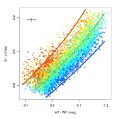
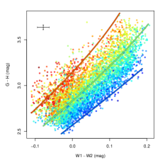
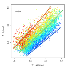
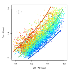
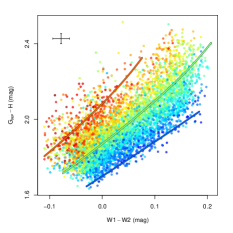
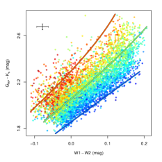
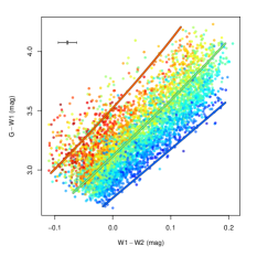
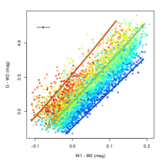
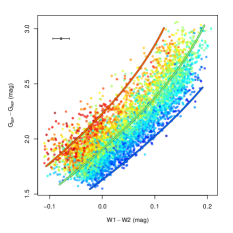
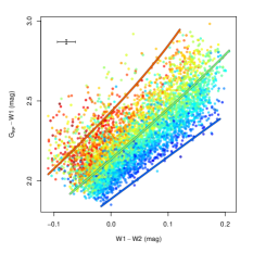
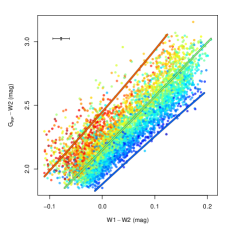
Figure A.1: Color–color diagrams of the stars from B20, color-coded by [Fe/H]${}_{\text{spec}}$, with the respective calibrations given by this work (red: $\text{[Fe/H]}=+0.3$, green: $\text{[Fe/H]}=0.0$, blue: $\text{[Fe/H]}=-0.3$). The mean uncertainties of the color indices involved are also shown in black in the bottom right corner of the panels.

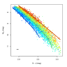
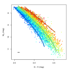
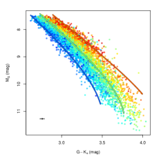
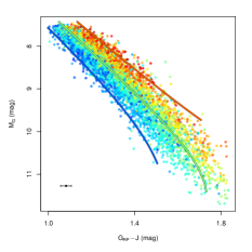
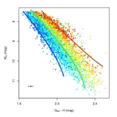
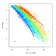
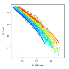
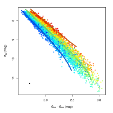
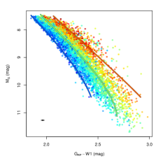
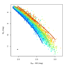
Figure A.2: Same as Fig. A.2 but for color–magnitude diagrams with $M_{G}$

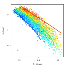
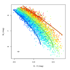
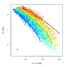
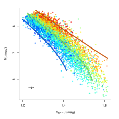
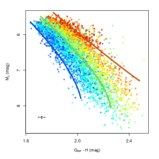
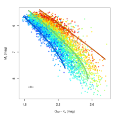
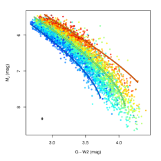
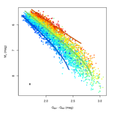
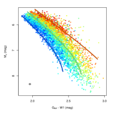
Figure A.3: Same as Fig. A.3 but for color–magnitude diagrams with $M_{J}$

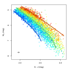
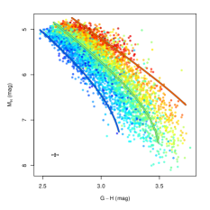
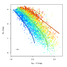
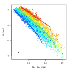
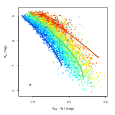
Figure A.4: Same as Fig. A.4 but for color–magnitude diagrams with $M_{H}$

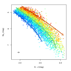
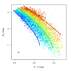
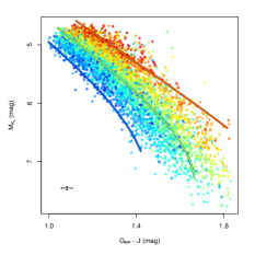
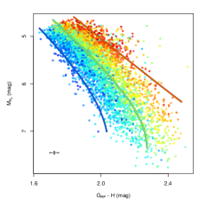
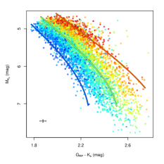
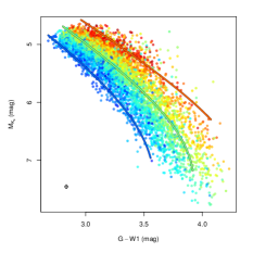
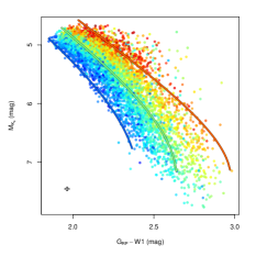
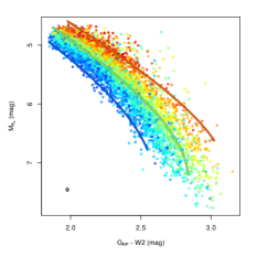
Figure A.5: Same as Fig. A.5 but for color–magnitude diagrams with $M_{K_{s}}$

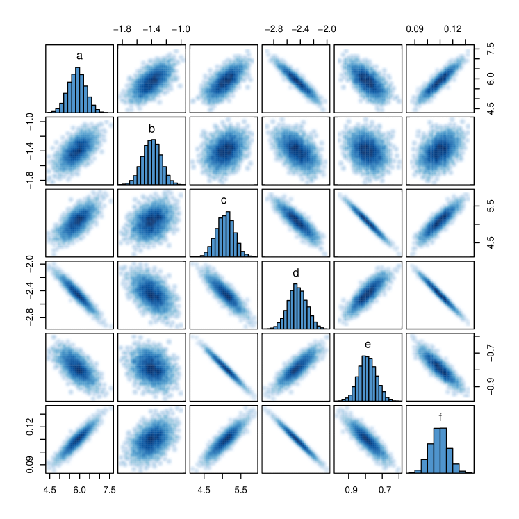
Figure A.6: Pairs plot of the coefficients corresponding to our best model: $W1-W2$ vs. $G_{\text{BP}}-G_{\text{RP}}$ vs. $M_{G}$.

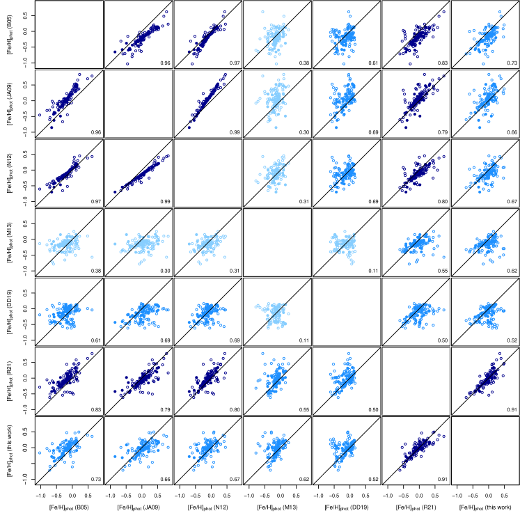
Figure A.7: Comparison between the different photometric estimations for the metallicity of the M-dwarf companions. The panels are color-coded by the correlation coefficient $r$ given in the bottom right corner (dark blue: $r\geq 0.75$; blue: $0.50\leq r<0.75$; light blue: $r<0.50$).

Appendix B Long table

Table B.1: Estimated metallicities of M-dwarf secondaries in FGK+M systems.

WDS	Name	$\alpha$	$\delta$	Sp.	[Fe/H]${}_{\text{spec}}$	[Fe/H]${}_{\text{phot}}$
				type	Montes+18	This work
J00467-0426	LP 646-9	00:46:43.4	$-$04:24:46	M4.0 V	$-0.10\pm 0.07$	$0.09\pm 0.08$
J01450-0104	LP 588-44	01:44:57.0	$-$01:03:04	M2.0	$-0.37\pm 0.03$	$-0.33\pm 0.08$
J02556+2652	HD 18143 C	02:55:35.8	$+$26:52:21	M4.0 V	$0.18\pm 0.05$	$0.16\pm 0.08$
J03078+2533	HD 19381B	03:07:58.3	$+$25:32:02	M3.5 V	$0.11\pm 0.02$	$0.11\pm 0.08$
J03203+0902	HD 20727B	03:20:42.5	$+$09:02:10	M4.0 V	$-0.24\pm 0.02$	$-0.03\pm 0.08$
J03356+4253	Wolf 191	03:35:28.5	$+$42:53:35	M0.5 V	$-0.37\pm 0.03$	$-0.43\pm 0.08$
J03520+3947	TYC 2868-639-1	03:51:58.1	$+$39:46:57	M0.0 V	$-0.13\pm 0.05$	$-0.03\pm 0.08$
J03556+5214	LSPM J0355+5214	03:55:36.9	$+$52:14:29	M2.5 V	$-0.32\pm 0.02$	$-0.32\pm 0.08$
J05003+2508	HD 31867B	05:00:19.5	$+$25:07:51	M1.0 V	$-0.01\pm 0.02$	$-0.02\pm 0.08$
J05264+0351	2MASS J05262029+0351111	05:26:20.3	$+$03:51:11	M1.5 V	$0.01\pm 0.03$	$-0.09\pm 0.08$
J05466+0110	HD 38529 B	05:46:19.4	$+$01:12:47	M2.5 V	$0.32\pm 0.02$	$0.23\pm 0.08$
J06319+0039	G 106-52	06:31:23.7	$+$00:36:45	M1.5 V	$-0.29\pm 0.02$	$-0.30\pm 0.08$
J06332+0528	HD 46375 B	06:33:12.1	$+$05:27:53	M2.0 V	$0.23\pm 0.06$	$0.23\pm 0.08$
J06461+3233	HD 263175 B	06:46:07.5	$+$32:33:15	M1.0 V	$-0.38\pm 0.03$	$-0.41\pm 0.08$
J07041+7514	LP 16-395	07:04:09.5	$+$75:14:37	M4.0 V	$0.18\pm 0.02$	$0.10\pm 0.08$
J08138+6306	NLTT 19115	08:14:19.0	$+$63:04:40	M1.5 V	$-0.09\pm 0.01$	$-0.19\pm 0.08$
J08484+2042	2MASS J08482492+2042188	08:48:24.9	$+$20:42:18	M1.5 V	$-0.03\pm 0.02$	$-0.14\pm 0.08$
J08492+0329	LEP 33	08:49:02.3	$+$03:29:47	M4	$0.05\pm 0.02$	$0.04\pm 0.08$
J09008+2347	HD 77052 B	09:00:53.2	$+$23:46:59	M2.5 V	$0.04\pm 0.02$	$-0.02\pm 0.08$
J09029+0600	2MASS J09025320+0602095	09:02:53.2	$+$06:02:10	M1.5 V	$-0.12\pm 0.02$	$-0.09\pm 0.08$
J09058+5532	NLTT 20915	09:05:51.2	$+$55:32:18	M3.5 V	$0.03\pm 0.02$	$-0.02\pm 0.08$
J09152+2323	BD+23 2063B	09:15:10.1	$+$23:21:33	M0.0 V	$0.21\pm 0.02$	$0.19\pm 0.08$
J11403+0931	LP 493-31	11:40:20.8	$+$09:30:45	M1.5 V	$-0.28\pm 0.03$	$-0.25\pm 0.08$
J11455+4740	G 122-46	11:47:21.7	$+$47:45:57	M2.5	$-0.45\pm 0.02$	$-0.31\pm 0.08$
J11523+0957	LP 493-64	11:52:17.9	$+$10:00:39	M4.0 V	$0.22\pm 0.06$	$0.16\pm 0.08$
J12051+1933	BD+20 2678B	12:05:11.9	$+$19:31:41	M2	$-0.07\pm 0.03$	$0.02\pm 0.08$
J12372+3545	2MASS J12371547+3549176	12:37:15.5	$+$35:49:18	M1.5 V	$-0.05\pm 0.02$	$-0.03\pm 0.08$
J13315-0800	HD 117579B	13:31:29.8	$-$07:59:59	M0.0 V	$-0.18\pm 0.02$	$-0.09\pm 0.08$
J14050+0157	NLTT 36190	14:04:55.8	$+$01:57:23	M2	$-0.01\pm 0.02$	$0.00\pm 0.08$
J14336+0920	HD 127871B	14:33:39.9	$+$09:20:10	M3.5 V	$-0.11\pm 0.03$	$-0.09\pm 0.08$
J14415+1336	HD 129290B	14:41:30.3	$+$13:37:36	M1.0 V	$-0.12\pm 0.02$	$-0.08\pm 0.08$
J15123+3939	LP 222-50	15:11:51.5	$+$39:33:02	M2.5 V	$-0.21\pm 0.03$	$-0.21\pm 0.08$
J15353+6005	LP 99-392	15:35:25.7	$+$60:05:08	M3.5 V	$-0.13\pm 0.06$	$-0.02\pm 0.08$
J16239+0315	G 17-23	16:33:02.8	$+$03:11:37	M3.0 V	$0.01\pm 0.04$	$0.00\pm 0.08$
J17428+1646	2MASS J17425203+1643476	17:42:52.0	$+$16:43:48	M1.5 V	$-0.23\pm 0.03$	$-0.21\pm 0.08$
J17477+2748	G 182-27	17:47:44.3	$+$27:47:07	M1.5 V	$-0.06\pm 0.02$	$0.00\pm 0.08$
J18006+6833	LDS 1460B	18:00:37.0	$+$68:32:54	K7 V	$-0.02\pm 0.02$	$0.00\pm 0.12$
J18006+2934	HD 164595B	18:00:45.4	$+$29:33:57	M2.0 V	$-0.08\pm 0.01$	$-0.09\pm 0.08$
J18090+2409	2MASS J18090192+2409041	18:09:01.9	$+$24:09:04	M1.0 V	$-0.13\pm 0.02$	$-0.11\pm 0.08$
J18292+1142	2MASS 18291369+1141271	18:29:13.7	$+$11:41:27	K5.0 V	$0.28\pm 0.02$	$0.21\pm 0.08$
J19321-1116	HD 183870B	19:32:08.1	$-$11:19:57	M3.5 V	$-0.10\pm 0.06$	$-0.02\pm 0.08$
J21324-2058	LP 873-74	21:32:21.0	$-$20:58:10	M0.5 V	$-0.19\pm 0.03$	$-0.15\pm 0.08$
J21575+2856	2MASS J21572970+2854494	21:57:29.7	$+$28:54:50	M1.5 V	$0.15\pm 0.02$	$0.10\pm 0.08$
J22090-1754	LP 819-37	22:08:54.2	$-$17:47:52	M2.5 V	$-0.42\pm 0.02$	$-0.28\pm 0.08$
J22159+5440	HD 211472B	22:16:02.6	$+$54:40:00	M4.0 V	$-0.05\pm 0.02$	$0.00\pm 0.08$
J22311+4509	HD 213519B	22:31:06.5	$+$45:09:44	M3	$0.00\pm 0.01$	$-0.06\pm 0.08$

References

- Abolfathi et al. (2018) Abolfathi, B., Aguado, D. S., Aguilar, G., et al. 2018, ApJS, 235, 42, doi: 10.3847/1538-4365/aa9e8a
- Adams & Laughlin (1997) Adams, F. C., & Laughlin, G. 1997, Reviews of Modern Physics, 69, 337, doi: 10.1103/RevModPhys.69.337
- Alam et al. (2015) Alam, S., Albareti, F. D., Allende Prieto, C., et al. 2015, ApJS, 219, 12, doi: 10.1088/0067-0049/219/1/12
- Allard et al. (1997) Allard, F., Hauschildt, P. H., Alexander, D. R., & Starrfield, S. 1997, ARA&A, 35, 137, doi: 10.1146/annurev.astro.35.1.137
- Alonso-Floriano et al. (2015) Alonso-Floriano, F. J., Morales, J. C., Caballero, J. A., et al. 2015, A&A, 577, A128, doi: 10.1051/0004-6361/201525803
- Andrews et al. (2018) Andrews, J. J., Chanamé, J., & Agüeros, M. A. 2018, MNRAS, 473, 5393, doi: 10.1093/mnras/stx2685
- Bahcall & Soneira (1980) Bahcall, J. N., & Soneira, R. M. 1980, ApJS, 44, 73, doi: 10.1086/190685
- Bergemann et al. (2017) Bergemann, M., Collet, R., Schönrich, R., et al. 2017, ApJ, 847, 16, doi: 10.3847/1538-4357/aa88b5
- Berger et al. (2006) Berger, D. H., Gies, D. R., McAlister, H. A., et al. 2006, ApJ, 644, 475, doi: 10.1086/503318
- Birky et al. (2020) Birky, J., Hogg, D. W., Mann, A. W., & Burgasser, A. 2020, ApJ, 892, 31, doi: 10.3847/1538-4357/ab7004
- Bonfils et al. (2005) Bonfils, X., Delfosse, X., Udry, S., et al. 2005, A&A, 442, 635, doi: 10.1051/0004-6361:20053046
- Bonnarel et al. (2000) Bonnarel, F., Fernique, P., Bienaymé, O., et al. 2000, A&AS, 143, 33, doi: 10.1051/aas:2000331
- Brewer et al. (2016) Brewer, J. M., Fischer, D. A., Valenti, J. A., & Piskunov, N. 2016, ApJS, 225, 32, doi: 10.3847/0067-0049/225/2/32
- Brooks & Gelman (1998) Brooks, S. P., & Gelman, A. 1998, Journal of Computational and Graphical Statistics, 7, 434, doi: 10.1080/10618600.1998.10474787
- Caballero et al. (2022) Caballero, J. A., González-Álvarez, E., Brady, M., et al. 2022, A&A, 665, A120, doi: 10.1051/0004-6361/202243548
- Carpenter et al. (2017) Carpenter, B., Gelman, A., Hoffman, M. D., et al. 2017, Journal of Statistical Software, 76, 1
- Cenarro et al. (2019) Cenarro, A. J., Moles, M., Cristóbal-Hornillos, D., et al. 2019, A&A, 622, A176, doi: 10.1051/0004-6361/201833036
- Chabrier (2003) Chabrier, G. 2003, PASP, 115, 763, doi: 10.1086/376392
- Cifuentes et al. (2020) Cifuentes, C., Caballero, J. A., Cortés-Contreras, M., et al. 2020, A&A, 642, A115, doi: 10.1051/0004-6361/202038295
- Cosentino et al. (2012) Cosentino, R., Lovis, C., Pepe, F., et al. 2012, in Society of Photo-Optical Instrumentation Engineers (SPIE) Conference Series, Vol. 8446, Ground-based and Airborne Instrumentation for Astronomy IV, ed. I. S. McLean, S. K. Ramsay, & H. Takami, 84461V, doi: 10.1117/12.925738
- Croswell (2002) Croswell, K. 2002, S&T, 104, 38
- Cutri et al. (2021) Cutri, R. M., Wright, E. L., Conrow, T., et al. 2021, VizieR Online Data Catalog, II/328
- Davenport & Dorn-Wallenstein (2019) Davenport, J. R. A., & Dorn-Wallenstein, T. Z. 2019, Research Notes of the American Astronomical Society, 3, 54, doi: 10.3847/2515-5172/ab11c9
- de Laverny et al. (2012) de Laverny, P., Recio-Blanco, A., Worley, C. C., & Plez, B. 2012, A&A, 544, A126, doi: 10.1051/0004-6361/201219330
- Delfosse et al. (2000) Delfosse, X., Forveille, T., Ségransan, D., et al. 2000, A&A, 364, 217. https://arxiv.org/abs/astro-ph/0010586
- Desidera et al. (2006) Desidera, S., Gratton, R. G., Lucatello, S., & Claudi, R. U. 2006, A&A, 454, 581, doi: 10.1051/0004-6361:20064896
- Dittmann et al. (2016) Dittmann, J. A., Irwin, J. M., Charbonneau, D., & Newton, E. R. 2016, ApJ, 818, 153, doi: 10.3847/0004-637X/818/2/153
- Duque-Arribas (2022) Duque-Arribas, C. 2022, METaMorPHosis: METallicity for M dwarfs using PHotometry, 1.0, Zenodo, doi: 10.5281/zenodo.7428860
- Engle & Guinan (2011) Engle, S. G., & Guinan, E. F. 2011, in Astronomical Society of the Pacific Conference Series, Vol. 451, 9th Pacific Rim Conference on Stellar Astrophysics, ed. S. Qain, K. Leung, L. Zhu, & S. Kwok, 285. https://arxiv.org/abs/1111.2872
- Espada (2019) Espada, A. 2019, M.Sc. thesis, Universidad Complutense de Madrid, Spain
- Ferguson et al. (2017) Ferguson, D., Gardner, S., & Yanny, B. 2017, ApJ, 843, 141, doi: 10.3847/1538-4357/aa77fd
- Fischer & Valenti (2005) Fischer, D. A., & Valenti, J. 2005, ApJ, 622, 1102, doi: 10.1086/428383
- Gaia Collaboration et al. (2016) Gaia Collaboration, Prusti, T., de Bruijne, J. H. J., et al. 2016, A&A, 595, A1, doi: 10.1051/0004-6361/201629272
- Gaia Collaboration et al. (2018a) Gaia Collaboration, Brown, A. G. A., Vallenari, A., et al. 2018a, A&A, 616, A1, doi: 10.1051/0004-6361/201833051
- Gaia Collaboration et al. (2018b) Gaia Collaboration, Babusiaux, C., van Leeuwen, F., et al. 2018b, A&A, 616, A10, doi: 10.1051/0004-6361/201832843
- Gaia Collaboration et al. (2021) Gaia Collaboration, Brown, A. G. A., Vallenari, A., et al. 2021, A&A, 649, A1, doi: 10.1051/0004-6361/202039657
- Gaia Collaboration et al. (2022) Gaia Collaboration, Vallenari, A., Brown, A. G. A., et al. 2022, arXiv e-prints, arXiv:2208.00211. https://arxiv.org/abs/2208.00211
- Gardner et al. (2006) Gardner, J. P., Mather, J. C., Clampin, M., et al. 2006, Space Sci. Rev., 123, 485, doi: 10.1007/s11214-006-8315-7
- Gelman et al. (2014) Gelman, A., Hwang, J., & Vehtari, A. 2014, Stat Comput, 24, 997 , doi: 10.1007/s11222-013-9416-2
- Gelman & Rubin (1992) Gelman, A., & Rubin, D. B. 1992, Statistical Science, 7, 457 , doi: 10.1214/ss/1177011136
- Gonzalez (1997) Gonzalez, G. 1997, MNRAS, 285, 403, doi: 10.1093/mnras/285.2.403
- Hejazi et al. (2015) Hejazi, N., De Robertis, M. M., & Dawson, P. C. 2015, AJ, 149, 140, doi: 10.1088/0004-6256/149/4/140
- Henry et al. (2006) Henry, T. J., Jao, W.-C., Subasavage, J. P., et al. 2006, AJ, 132, 2360, doi: 10.1086/508233
- Hobson et al. (2018) Hobson, M. J., Jofré, E., García, L., Petrucci, R., & Gómez, M. 2018, Rev. Mexicana Astron. Astrofis., 54, 65. https://arxiv.org/abs/1711.04878
- Irwin et al. (2015) Irwin, J. M., Berta-Thompson, Z. K., Charbonneau, D., et al. 2015, in Cambridge Workshop on Cool Stars, Stellar Systems, and the Sun, Vol. 18, 18th Cambridge Workshop on Cool Stars, Stellar Systems, and the Sun, 767–772. https://arxiv.org/abs/1409.0891
- Ishikawa et al. (2020) Ishikawa, H. T., Aoki, W., Kotani, T., et al. 2020, PASJ, 72, 102, doi: 10.1093/pasj/psaa101
- Jeffers et al. (2018) Jeffers, S. V., Schöfer, P., Lamert, A., et al. 2018, A&A, 614, A76, doi: 10.1051/0004-6361/201629599
- Johnson & Apps (2009) Johnson, J. A., & Apps, K. 2009, ApJ, 699, 933, doi: 10.1088/0004-637X/699/2/933
- Johnson et al. (2012) Johnson, J. A., Gazak, J. Z., Apps, K., et al. 2012, AJ, 143, 111, doi: 10.1088/0004-6256/143/5/111
- Jones et al. (2005) Jones, H. R. A., Pavlenko, Y., Viti, S., et al. 2005, MNRAS, 358, 105, doi: 10.1111/j.1365-2966.2005.08736.x
- Kiman et al. (2021) Kiman, R., Faherty, J. K., Cruz, K. L., et al. 2021, AJ, 161, 277, doi: 10.3847/1538-3881/abf561
- Kopparapu et al. (2014) Kopparapu, R. K., Ramirez, R. M., SchottelKotte, J., et al. 2014, ApJ, 787, L29, doi: 10.1088/2041-8205/787/2/L29
- Kotani et al. (2018) Kotani, T., Tamura, M., Nishikawa, J., et al. 2018, in Society of Photo-Optical Instrumentation Engineers (SPIE) Conference Series, Vol. 10702, Ground-based and Airborne Instrumentation for Astronomy VII, ed. C. J. Evans, L. Simard, & H. Takami, 1070211, doi: 10.1117/12.2311836
- Kruschke (2014) Kruschke, J. K. 2014, Doing Bayesian Data Analysis: A Tutorial with R, JAGS, and Stan (2nd edition), ISBN 978-0-12-405888-0
- Laureijs et al. (2011) Laureijs, R., Amiaux, J., Arduini, S., et al. 2011, arXiv e-prints, arXiv:1110.3193. https://arxiv.org/abs/1110.3193
- Lindegren et al. (2021) Lindegren, L., Klioner, S. A., Hernández, J., et al. 2021, A&A, 649, A2, doi: 10.1051/0004-6361/202039709
- López-Morales (2007) López-Morales, M. 2007, ApJ, 660, 732, doi: 10.1086/513142
- López-Morales & Ribas (2005) López-Morales, M., & Ribas, I. 2005, ApJ, 631, 1120, doi: 10.1086/432680
- Luque et al. (2019) Luque, R., Pallé, E., Kossakowski, D., et al. 2019, A&A, 628, A39, doi: 10.1051/0004-6361/201935801
- Mahadevan et al. (2012) Mahadevan, S., Ramsey, L., Bender, C., et al. 2012, in Society of Photo-Optical Instrumentation Engineers (SPIE) Conference Series, Vol. 8446, Ground-based and Airborne Instrumentation for Astronomy IV, ed. I. S. McLean, S. K. Ramsay, & H. Takami, 84461S, doi: 10.1117/12.926102
- Majewski et al. (2017) Majewski, S. R., Schiavon, R. P., Frinchaboy, P. M., et al. 2017, AJ, 154, 94, doi: 10.3847/1538-3881/aa784d
- Mann et al. (2013) Mann, A. W., Brewer, J. M., Gaidos, E., Lépine, S., & Hilton, E. J. 2013, AJ, 145, 52, doi: 10.1088/0004-6256/145/2/52
- Mann et al. (2015) Mann, A. W., Feiden, G. A., Gaidos, E., Boyajian, T., & von Braun, K. 2015, ApJ, 804, 64, doi: 10.1088/0004-637X/804/1/64
- Mann et al. (2019) Mann, A. W., Dupuy, T., Kraus, A. L., et al. 2019, ApJ, 871, 63, doi: 10.3847/1538-4357/aaf3bc
- Marfil et al. (2021) Marfil, E., Tabernero, H. M., Montes, D., et al. 2021, A&A, 656, A162, doi: 10.1051/0004-6361/202141980
- Marocco et al. (2021) Marocco, F., Eisenhardt, P. R. M., Fowler, J. W., et al. 2021, ApJS, 253, 8, doi: 10.3847/1538-4365/abd805
- Martínez-Rodríguez et al. (2019) Martínez-Rodríguez, H., Caballero, J. A., Cifuentes, C., Piro, A. L., & Barnes, R. 2019, ApJ, 887, 261, doi: 10.3847/1538-4357/ab5640
- Mayor et al. (2003) Mayor, M., Pepe, F., Queloz, D., et al. 2003, The Messenger, 114, 20
- Medan et al. (2021) Medan, I., Lépine, S., & Hartman, Z. 2021, AJ, 161, 234, doi: 10.3847/1538-3881/abe878
- Montes et al. (2018) Montes, D., González-Peinado, R., Tabernero, H. M., et al. 2018, MNRAS, 479, 1332, doi: 10.1093/mnras/sty1295
- Morales et al. (2019) Morales, J. C., Mustill, A. J., Ribas, I., et al. 2019, Science, 365, 1441, doi: 10.1126/science.aax3198
- Ness et al. (2015) Ness, M., Hogg, D. W., Rix, H. W., Ho, A. Y. Q., & Zasowski, G. 2015, ApJ, 808, 16, doi: 10.1088/0004-637X/808/1/16
- Neves et al. (2012) Neves, V., Bonfils, X., Santos, N. C., et al. 2012, A&A, 538, A25, doi: 10.1051/0004-6361/201118115
- Nutzman & Charbonneau (2008) Nutzman, P., & Charbonneau, D. 2008, PASP, 120, 317, doi: 10.1086/533420
- Olander et al. (2021) Olander, T., Heiter, U., & Kochukhov, O. 2021, A&A, 649, A103, doi: 10.1051/0004-6361/202039747
- Passegger et al. (2018) Passegger, V. M., Reiners, A., Jeffers, S. V., et al. 2018, A&A, 615, A6, doi: 10.1051/0004-6361/201732312
- Passegger et al. (2020) Passegger, V. M., Bello-García, A., Ordieres-Meré, J., et al. 2020, A&A, 642, A22, doi: 10.1051/0004-6361/202038787
- Passegger et al. (2022) —. 2022, A&A, 658, A194, doi: 10.1051/0004-6361/202141920
- Pepe et al. (2021) Pepe, F., Cristiani, S., Rebolo, R., et al. 2021, A&A, 645, A96, doi: 10.1051/0004-6361/202038306
- Pepe et al. (2010) Pepe, F. A., Cristiani, S., Rebolo Lopez, R., et al. 2010, in Society of Photo-Optical Instrumentation Engineers (SPIE) Conference Series, Vol. 7735, Ground-based and Airborne Instrumentation for Astronomy III, ed. I. S. McLean, S. K. Ramsay, & H. Takami, 77350F, doi: 10.1117/12.857122
- Quirrenbach et al. (2020) Quirrenbach, A., CARMENES Consortium, Amado, P. J., et al. 2020, in Society of Photo-Optical Instrumentation Engineers (SPIE) Conference Series, Vol. 11447, Society of Photo-Optical Instrumentation Engineers (SPIE) Conference Series, 114473C, doi: 10.1117/12.2561380
- Rains et al. (2021) Rains, A. D., Žerjal, M., Ireland, M. J., et al. 2021, MNRAS, 504, 5788, doi: 10.1093/mnras/stab1167
- Raskin et al. (2011) Raskin, G., van Winckel, H., Hensberge, H., et al. 2011, A&A, 526, A69, doi: 10.1051/0004-6361/201015435
- Reid et al. (1997) Reid, I. N., Gizis, J. E., Cohen, J. G., et al. 1997, PASP, 109, 559, doi: 10.1086/133914
- Reiners et al. (2018) Reiners, A., Zechmeister, M., Caballero, J. A., et al. 2018, A&A, 612, A49, doi: 10.1051/0004-6361/201732054
- Reylé et al. (2021) Reylé, C., Jardine, K., Fouqué, P., et al. 2021, A&A, 650, A201, doi: 10.1051/0004-6361/202140985
- Ricker et al. (2014) Ricker, G. R., Winn, J. N., Vanderspek, R., et al. 2014, in Society of Photo-Optical Instrumentation Engineers (SPIE) Conference Series, Vol. 9143, Space Telescopes and Instrumentation 2014: Optical, Infrared, and Millimeter Wave, ed. J. Oschmann, Jacobus M., M. Clampin, G. G. Fazio, & H. A. MacEwen, 914320, doi: 10.1117/12.2063489
- Riello et al. (2021) Riello, M., De Angeli, F., Evans, D. W., et al. 2021, A&A, 649, A3, doi: 10.1051/0004-6361/202039587
- Rojas-Ayala et al. (2010) Rojas-Ayala, B., Covey, K. R., Muirhead, P. S., & Lloyd, J. P. 2010, ApJ, 720, L113, doi: 10.1088/2041-8205/720/1/L113
- Rojas-Ayala et al. (2012) —. 2012, ApJ, 748, 93, doi: 10.1088/0004-637X/748/2/93
- Sarmento et al. (2020) Sarmento, P., Delgado Mena, E., Rojas-Ayala, B., & Blanco-Cuaresma, S. 2020, A&A, 636, A85, doi: 10.1051/0004-6361/201936296
- Schlaufman & Laughlin (2010) Schlaufman, K. C., & Laughlin, G. 2010, A&A, 519, A105, doi: 10.1051/0004-6361/201015016
- Schmidt et al. (2016) Schmidt, S. J., Wagoner, E. L., Johnson, J. A., et al. 2016, MNRAS, 460, 2611, doi: 10.1093/mnras/stw1139
- Schwab et al. (2016) Schwab, C., Rakich, A., Gong, Q., et al. 2016, in Society of Photo-Optical Instrumentation Engineers (SPIE) Conference Series, Vol. 9908, Ground-based and Airborne Instrumentation for Astronomy VI, ed. C. J. Evans, L. Simard, & H. Takami, 99087H, doi: 10.1117/12.2234411
- Schweitzer et al. (2019) Schweitzer, A., Passegger, V. M., Cifuentes, C., et al. 2019, A&A, 625, A68, doi: 10.1051/0004-6361/201834965
- Seifahrt et al. (2020) Seifahrt, A., Bean, J. L., Stürmer, J., et al. 2020, in Society of Photo-Optical Instrumentation Engineers (SPIE) Conference Series, Vol. 11447, Society of Photo-Optical Instrumentation Engineers (SPIE) Conference Series, 114471F, doi: 10.1117/12.2561564
- Shetrone et al. (2015) Shetrone, M., Bizyaev, D., Lawler, J. E., et al. 2015, ApJS, 221, 24, doi: 10.1088/0067-0049/221/2/24
- Shields et al. (2016) Shields, A. L., Ballard, S., & Johnson, J. A. 2016, Phys. Rep., 663, 1, doi: 10.1016/j.physrep.2016.10.003
- Skrutskie et al. (2006) Skrutskie, M. F., Cutri, R. M., Stiening, R., et al. 2006, AJ, 131, 1163, doi: 10.1086/498708
- Stauffer & Hartmann (1986) Stauffer, J. R., & Hartmann, L. W. 1986, ApJS, 61, 531, doi: 10.1086/191123
- Tabernero et al. (2019) Tabernero, H. M., Marfil, E., Montes, D., & González Hernández, J. I. 2019, A&A, 628, A131, doi: 10.1051/0004-6361/201935465
- Tarter et al. (2007) Tarter, J. C., Backus, P. R., Mancinelli, R. L., et al. 2007, Astrobiology, 7, 30, doi: 10.1089/ast.2006.0124
- Taylor (2005) Taylor, M. B. 2005, in Astronomical Society of the Pacific Conference Series, Vol. 347, Astronomical Data Analysis Software and Systems XIV, ed. P. Shopbell, M. Britton, & R. Ebert, 29
- Terrien et al. (2012) Terrien, R. C., Mahadevan, S., Bender, C. F., et al. 2012, ApJ, 747, L38, doi: 10.1088/2041-8205/747/2/L38
- Trifonov et al. (2018) Trifonov, T., Kürster, M., Zechmeister, M., et al. 2018, A&A, 609, A117, doi: 10.1051/0004-6361/201731442
- Van Eck et al. (2017) Van Eck, S., Neyskens, P., Jorissen, A., et al. 2017, A&A, 601, A10, doi: 10.1051/0004-6361/201525886
- Vehtari et al. (2017) Vehtari, A., Gelman, A., & Gabry, J. 2017, Stat Comput, 27, 1413–1432, doi: 10.1007/s11222-016-9696-4
- Vehtari et al. (2015) Vehtari, A., Simpson, D., Gelman, A., Yao, Y., & Gabry, J. 2015, arXiv e-prints, arXiv:1507.02646. https://arxiv.org/abs/1507.02646
- West et al. (2008) West, A. A., Hawley, S. L., Bochanski, J. J., et al. 2008, AJ, 135, 785, doi: 10.1088/0004-6256/135/3/785
- Winters et al. (2015) Winters, J. G., Henry, T. J., Lurie, J. C., et al. 2015, AJ, 149, 5, doi: 10.1088/0004-6256/149/1/5
- Wright et al. (2010) Wright, E. L., Eisenhardt, P. R. M., Mainzer, A. K., et al. 2010, AJ, 140, 1868, doi: 10.1088/0004-6256/140/6/1868
- Zechmeister et al. (2019) Zechmeister, M., Dreizler, S., Ribas, I., et al. 2019, A&A, 627, A49, doi: 10.1051/0004-6361/201935460