Global Nash Equilibrium in Non-convex Multi-player Game: Theory and Algorithms

Abstract

Wide machine learning tasks can be formulated as non-convex multi-player games, where Nash equilibrium (NE) is an acceptable solution to all players, since no one can benefit from changing its strategy unilaterally. Attributed to the non-convexity, obtaining the existence condition of global NE is challenging, let alone designing theoretically guaranteed realization algorithms. This paper takes conjugate transformation to the formulation of non-convex multi-player games, and casts the complementary problem into a variational inequality (VI) problem with a continuous pseudo-gradient mapping. We then prove the existence condition of global NE: the solution to the VI problem satisfies a duality relation. Based on this VI formulation, we design a conjugate-based ordinary differential equation (ODE) to approach global NE, which is proved to have an exponential convergence rate. To make the dynamics more implementable, we further derive a discretized algorithm. We apply our algorithm to two typical scenarios: multi-player generalized monotone game and multi-player potential game. In the two settings, we prove that the step-size setting is required to be $\mathcal{O}(1/k)$ and $\mathcal{O}(1/\sqrt{k})$ to yield the convergence rates of $\mathcal{O}(1/k)$ and $\mathcal{O}(1/\sqrt{k})$, respectively. Extensive experiments in robust neural network training and sensor localization are in full agreement with our theory.

1 Introduction

Many advanced learning approaches in artificial intelligence are developed toward multi-agent ways, distributed manners, or federated frameworks [yu2019multi, li2019interaction, fan2021fault, zhu2022topology]. For instance, as one of the most popular schemes, adversarial learning is gradually generalized to multiple agents [song2018multi, zhao2020improving, 9613799], not restricted to classic models with one generator and one discriminator. Also, most complex systems involve the interaction and interference of the multiple participants therein, such as smart grids [saad2012game], intelligent transportation [saharan2020dynamic], and cloud computing [pang2008distributed]. The common core ideology is to sufficiently utilize the autonomy and evolvability of individual computational units in large-scale tasks. General optimization frameworks or min-max adversarial protocols will be no longer evergreen, and proper models should be established for describing these multi-agent systems as well as the accompanied solvers.

Game theory exploits the advantages to the full in such multi-player scenarios. Actually, game theory has been playing an essential role in the leading edge of machine learning nowadays such as adversarial training and reinforcement learning [busoniu2008comprehensive, lanctot2017unified, dai2018sbeed, 6330964]. The Nash equilibrium (NE) therein [nash1951non] becomes a popular concept in various fields like applied mathematics, computer sciences, and engineering, in addition to economy. When all players’ strategy profile reaches an NE, no one can benefit from changing its strategy unilaterally. This paper focuses on a typical class of non-convex multi-player games. Player $i$ minimizes its own payoff function $J_{i}(x_{i},\bm{x}_{-i}):\mathbb{R}^{Nn}\rightarrow\mathbb{R}$, which is influenced by both the player’s own decision $x_{i}\in\mathbb{R}^{n}$ and others’ decisions $\bm{x}_{-i}\in\mathbb{R}^{(N-1)n}$. Specifically, the non-convex structure in players’ payoff is endowed with

$$J_{i}(x_{i},\bm{x}_{-i})=\Psi_{i}(\Lambda_{i}(x_{i},\bm{x}_{-i})).$$

Here, $\Lambda_{i}:\mathbb{R}^{Nn}\rightarrow\mathbb{R}^{q_{i}}$ is a vector-valued nonlinear operator, where $\Lambda_{i}=(\Lambda_{i,1},\cdots,\Lambda_{i,q_{i}})^{T}$ and for $k\in\{1,\cdots,q_{i}\}$, $\Lambda_{i,k}:\mathbb{R}^{Nn}\rightarrow\mathbb{R}$ is a quadratic function in $x_{i}$. Besides, $\Psi_{i}:\mathbb{R}^{q_{i}}\rightarrow\mathbb{R}$ is a canonical function [gao2017canonical], whose gradient $\nabla\Psi_{i}$ is a one-to-one mapping from the primal space into the dual space.

This setting has been widely investigated in machine learning applications, such as robust network training and sensor network localization. For example, in sensor localization [ke2017distributed, yang2018df], $x_{i}$ is the sensor node, $\Lambda_{i,k}$ represents the estimated distance between $x_{i}$ and $\bm{x}_{-i}$, while $\Psi_{i}$ is reified as Euclidean norms to measure the error of the true distance and the estimated distance. In robust neural network training [nouiehed2019solving, deng2021local], $x_{i}$ denotes the model parameter, $\Lambda_{i,k}$ serves as the output of training data, while $\Psi_{i}$ represents the cross-entropy function. Moreover, this setting may also inspire solutions to resource allocation problems in unmanned vehicles [yang2019energy] and secure transmission [ruby2015centralized], where $x_{i}$ stands for the transmit resources, $\Psi_{i}$ denotes the transmission cost together with $\Lambda_{i,k}$, which is a logarithmic-posynomial function.

Given the above formulation, it is natural and essential from both game-theoretic and machine-learning perspectives to seek its global NE, which characterizes a global optimum solution since no one will deviate from its strategy unilaterally with others’ given strategies. However, it is the status quo that finding the global optimum or equilibrium in non-convex settings is still an open problem [1177151, 8643982, 9398583]. That is not only owing to the lack of powerful tools compared with convex categories, but also due to the diversity of non-convex structures, which may not be solved by a common methodology. Despite many efficient tools within convex conditions leading to fruitful achievements of multi-player game models [yi2019operator, chen2021distributed, facchinei2010penalty], they may be far from enough when encountering the non-convexity, and may be stuck in local NE or approximations when tracking along the pseudo-gradients, rather than reaching a global NE. On the other hand, although some inspiring breakthroughs have been made for solving non-convex two-player min-max games in different situations, such as Polyak-Łojasiewicz cases [nouiehed2019solving, fiez2021global], concave cases [lin2020gradient, rafique2021weakly], they may not provide available help in multi-player settings, because the global stationary conditions are mutually coupled and cannot be handled individually by each player. Thus, we need novel processes to explore the existence of global NE and design algorithms to realize it.

To this end, we first employ the canonical duality theory [gao2017canonical] and obtain a one-to-one duality relation within a conjugate transformation [rockafellar1974conjugate], in order to deal with the non-convexity in payoff functions. By generalizing to continuous vector fields, we compactly formulate the coupled stationary conditions of the transformed problem as a continuous mapping. Thus, seeking all players’ NE profile can be accomplished by verifying a fixed point of this continuous mapping. We then cast the fixed point seeking into solving a variational inequality (VI) problem [facchinei2003finite]. By the above procedures, we can transform the global NE of a non-convex multi-player game into the solution to a VI problem, which is much easier to be solved since all players’ coupled stationary conditions are regarded from an entire perspective. So far, we obtain the existence condition of the global NE in such a non-convex multi-player game: the solution to the VI problem is required to satisfy the duality relation.

Based on this transformation, we then propose a conjugate-based ordinary differential equation (ODE) for solving the VI problem. No longer flowing in the primal spaces, the ODE evolves in the dual spaces of both decision variables and canonical variables. Then a mapping from this dual space to the primal space is enforced via the gradient information of differentiable Legendre conjugate functions [diakonikolas2019approximate]. We prove that the equilibrium of this conjugate-based ODE is the global NE of this non-convex multi-player game if the aforementioned existence condition is verified. Besides, we provide rigorous convergence analysis on the continuous dynamics, as well as prove that the ODE has an exponential convergence rate.

For practical implementation, we further derive a discrete algorithm associated with the proposed conjugate-based ODE. We analyze the step-size settings for some desired convergence rates in two typical non-convex game models. Specifically, with a step size as $\mathcal{O}(1/k)$, the convergence rate achieves $\mathcal{O}(1/k)$ in a class of multi-player generalized monotone games [facchinei2010penalty, koshal2016distributed]; while with another step size as $\mathcal{O}(1/\sqrt{k})$, the convergence rate achieves $\mathcal{O}(1/\sqrt{k})$ in a class of multi-player potential games [ke2017distributed, yang2018df].

We conduct extensive experiments in robust neural network training and sensor localization. All these experimental results show that our algorithm converges to the global NE of non-convex games, instead of being stuck in local NE or approximate NE. Moreover, we compare our algorithm against several popular methods on these multi-player settings and demonstrate that our algorithm outperforms all other techniques.

To our best knowledge, this is the first paper on the existence condition and realization algorithms of the global Nash equilibria in a non-convex multi-player game. Our contributions are summarised below:

• Existence condition. We employ canonical duality theory to transform the non-convex multi-player game into a complementary dual problem, and cast solving all players’ stationary point profile into solving a VI problem. Then we provide the existence condition of global NE: the solution to the VI problem is required to satisfy a duality relation.

• Conjugate-based ODE. We propose a conjugate-based ODE for solving the VI problem, which evolves in the dual spaces of both decision variables and canonical variables. The equilibrium of the ODE is the global NE of this non-convex multi-player game if the existence condition is verified. The convergence analysis of the ODE and its exponential convergence rate are provided.

• Discrete algorithm. We derive a discrete algorithm based on the continuous ODE for practical implementation in two typical non-convex scenarios – a convergence rate of $\mathcal{O}(1/k)$ in a class of multi-player generalized monotone games with a step size of $\mathcal{O}(1/k)$, and another convergence rate of $\mathcal{O}(1/\sqrt{k})$ in a class of multi-player potential games with a step size of $\mathcal{O}(1/\sqrt{k})$.

The rest of this paper is organized as follows: Section 2 introduces the related work. Section 3 formulates a non-convex multi-player game, while Section 4 investigates the existence of global NE. Section 5 proposes an ODE to seek the global NE and gives the exponential convergence analysis. Section LABEL:d5 derives a discretized algorithm from the ODE and presents the step-size settings and convergence rates in two typical scenarios. Section LABEL:e11 examines the effectiveness of the proposed approach with several experiments. Section LABEL:discuss gives some discussions on the results of theory and algorithms obtained in this paper. Finally, Section LABEL:conclusion concludes the paper and gives some future directions.

2 Related Work

Convex multi-player games. Many theoretical results in multi-player games have been built on fundamental convexity assumptions [facchinei2010penalty, yi2019operator, chen2021distributed]. Under the frame of convexity, NE seeking has been extensively studied in many typical multi-player game models, including aggregative games [koshal2016distributed, xu2022efficient], potential games [lei2020asynchronous, yang2018df], and hierarchical games [kim2001hierarchical]. For example, [facchinei2010penalty, lei2020asynchronous] directly required convex payoffs on each player’s decision variable, while [koshal2016distributed, chen2021distributed] needs strongly/strictly monotone pseudo gradients to display the interaction on all players’ actions. Despite many efficient tools within convex conditions leading to fruitful achievements, they may be far from enough when encountering non-convexity in practical circumstances.

Non-convex two-player min-max problems. Some inspiring breakthroughs have been achieved for solving non-convex two-player min-max problems, including Polyak-Łojasiewicz cases [nouiehed2019solving, fiez2021global], strongly-concave cases [lin2020gradient, rafique2021weakly], and general non-convex non-concave cases [heusel2017gans, daskalakis2018limit]. Such popular researches owe to the success of GAN and its variants [goodfellow2014generative, daskalakis2018training]. For instance, [heusel2017gans] proposed a two time-scale update rule with stochastic gradient descent to find a local NE in GANs, while [daskalakis2018limit] designed an optimistic mirror descent algorithm to explore NE in GANs with a theoretical guarantee. However, it is not straightforward and realistic to directly generalize the above two-player approaches to solve multi-player settings. It is because the global stationary conditions are mutually coupled among multiple players and cannot be handled individually, which is unlike two-player situations.

Non-convex multi-player games with local NE or approximations. Initial efforts have been made for solving non-convex multi-player games. [pang2011nonconvex] proposed a best-response scheme for Nash stationary points of a class of non-convex games in signal processing, and then [hao2020piecewise] extended this method in multi-player bilevel games with non-convex constraints. Moreover, [raghunathan2019game] introduced a gradient-based Nikaido-Isoda function to find Nash stationary points in a reformulated non-convex game, while [liu2020approximate] designed a gradient-proximal algorithm for approximate NE in a class of non-convex aggregative games. The algorithms within these works lead to local NE or Nash stationary points dependent on the initial points. How to guarantee the existence of global NE and how to design algorithms for seeking global NE deserve further investigation in non-convex multi-player game models.

Similar non-convex structures in optimization. Related results exist in solving such non-convex problems where the objectives or payoffs are composited with canonical functions and quadratic operators, which are however somewhat premature. [zhu2012approximate] considered an approximate optimization to relax such non-convex constraints and provided the optimality conditions for the simplified problem, while [latorre2016canonical] proposed similar sufficient conditions and discussed the existence of the global optimum via canonical duality theory. On this basis, [ren2021distributed] investigated the global optimal solution of such a non-convex optimization in a distributed manner over multi-agent networks, while [liang2019topology] focused on approximating the solutions of discrete variable topology problems with multiple constraints. We notice that regarded as so important a class of non-convex problems, most of the existing work concentrated on the optimization perspective. Taking into account the interference and interaction among multiple players, the global stationary conditions are mutually coupled and can not be handled individually by each player. Therefore, the above optimization methods cannot completely match our problems. Serving as a widely accepted equilibrium concept, the global NE therein needs to be further discussed with respect to its existence conditions and seeking algorithms. The consequent results in this paper will help demystify the complicated interactions among players and provide trustworthy insights for large-scale problems afterward.

3 Preliminaries on Game Theory

We begin our study of the non-convex games with multiple players indexed by $\mathcal{I}=\{1,\cdots,N\}$. For $i\in\mathcal{I}$, the $i$th player has an action variable $x_{i}$ in an action set $\Omega_{i}\subseteq\mathbb{R}^{n}$, where $\Omega_{i}$ is compact and convex, and $\bm{\Omega}=\prod_{i=1}^{N}\Omega_{i}$. Let $\bm{x}=\operatorname{col}\{x_{1},...,x_{N}\}\in\mathbb{R}^{nN}$ be the profile of all players’ actions, while $\bm{x}_{-i}$ be the profile of all players’ actions except for the $i$th player’s. Moreover, the $i$th player has a payoff function $J_{i}(x_{i},\bm{x}_{-i}):\bm{\Omega}\rightarrow\mathbb{R}$, which is dependent on both $x_{i}$ and $\bm{x}_{-i}$, and twice continuously differentiable in $x_{i}$. Given $\bm{x}_{-i}$, the $i$th player intends to solve the following problem

$$\min\limits_{x_{i}}J_{i}\left(x_{i},\bm{x}_{-i}\right),\quad\text{s.t. }x_{i}\in\Omega_{i}.$$ (1)

In this paper, we focus on a typical class of non-convex multi-player games, in which the $i$th player’s payoff function is endowed with the following structure

$$J_{i}(x_{i},\bm{x}_{-i})=\Psi_{i}(\Lambda_{i}(x_{i},\bm{x}_{-i})).$$ (2)

Here $\Lambda_{i}:\mathbb{R}^{Nn}\rightarrow\Theta_{i}\subseteq\mathbb{R}^{q_{i}}$ is a vector-valued nonlinear operator with $\Lambda_{i}=(\Lambda_{i,1},\cdots,\Lambda_{i,q_{i}})^{T}$. For $k\in\{1,\cdots,q_{i}\}$, each $\Lambda_{i,k}:\mathbb{R}^{Nn}\rightarrow\mathbb{R}$ is quadratic in $x_{i}$, whose second-order partial derivative in $x_{i}$ is both $x_{i}$-free and $\bm{x}_{-i}$-free, e.g., $\Lambda_{i,k}=x_{i}^{T}A_{i,k}x_{i}+\sum_{i\neq j}x_{i}^{T}B_{i,k}x_{j}$. Moreover, $\Psi_{i}:\Theta_{i}\rightarrow\mathbb{R}$ is a convex differential canonical function [gao2017canonical], whose gradient $\nabla\Psi_{i}:\Theta_{i}\rightarrow\Theta^{*}_{i}$ is a one-to-one mapping. Such non-convex structures composited by canonical functions and quadratic operators emerge in broad applications, including robust network training [nouiehed2019solving], sensor localization [yang2018df], and GAN [gidel2018variational]. We provide specific examples in the following for intuition about the above non-convex model.

Example 1 (Euclidian distance function)

$$\sum\nolimits_{j\in\mathcal{N}_{i}}(\left\|x_{i}-{x}_{j}\right\|^{2}-d_{i,j})^{2},$$ (3)

where $\Psi_{i}=\sum\nolimits_{j=1}\nolimits^{\mathcal{N}_{i}}\Lambda_{i,j}^{T}\Lambda_{i,j}$ and $\Lambda_{i,j}=\left\|x_{i}-{x}_{j}\right\|^{2}-d_{i,j}$. (3) usually serves as the payoffs in sensor localization [jia2013distributed, ke2017distributed, yang2018df], where $x_{i}\in\Omega_{i}$ is a sensor node, $\mathcal{N}_{i}$ is the neighbors of node $i$, and $d_{i,j}$ is the distance parameter.

Example 2 (Log-sum-exp function)

$$\beta_{1}\log[1+\exp(-x_{i}^{T}x_{i}-\sum\nolimits_{j=1}^{N}x_{i}^{{T}}x_{j}-\beta_{2}^{{T}}x_{i})],$$ (4)

where $\Psi_{i}=\beta_{1}\log[1+\exp\Lambda_{i}]$ and $\Lambda_{i}=-x_{i}^{T}x_{i}-\sum\nolimits_{j=1}^{N}x_{i}^{{T}}x_{j}-\beta_{2}^{{T}}x_{i}$. (4) usually appears in the tasks like robust neural network training [nouiehed2019solving, deng2021local], where $x_{i}$ is the neural network parameter, $x_{j}$ is the perturbation, and $\beta_{1},\beta_{2}$ are training data.

Example 3 (Log-posynomial function)

$$\log(x_{i}^{T}\mathbf{C}_{i}x_{i}+x_{i}^{T}\mathbf{D}_{i}\bm{x}_{-i})^{-1},$$ (5)

where $\Psi_{i}=\log(\Lambda_{i})^{-1}$ and $\Lambda_{i}=x_{i}^{T}\mathbf{C}_{i}x_{i}+x_{i}^{T}\mathbf{D}_{i}\bm{x}_{-i}$. (5) usually occurs in resource allocation [yang2019energy, ruby2015centralized, chiang2007power], where $x_{i}$ stands for transmitting resources, and matrices $\mathbf{C}_{i}$ and $\mathbf{D}_{i}$ represent the correlation coefficients.

We introduce the following important concept for solving the non-convex multi-player game (1).

Definition 1 (global Nash equilibrium)

A strategy profile $\bm{x}^{\Diamond}\in\bm{\Omega}$ is said to be a global Nash equilibrium (NE) of (1), if for all $i\in\mathcal{I}$,

$$J_{i}(x_{i}^{\Diamond},\bm{x}_{-i}^{\Diamond})\leq J_{i}(x_{i},\bm{x}_{-i}^{\Diamond}),\quad\forall x_{i}\in\Omega_{i}.$$ (6)

The global NE above characterizes a strategy profile that each player adopts its globally optimal strategy. That is, given others’ actions, no player can benefit from changing her/his action unilaterally. Actually, the conception of global NE here is indeed the concept of NE [nash1951non], and we emphasize global in the non-convex formulation to tell the difference from local NE [pang2011nonconvex, nouiehed2019solving, heusel2017gans]. Also, we consider another mild but well-known concept to help characterize the solutions to (1).

Definition 2 (Nash stationary point)

A strategy profile $\bm{x}^{\Diamond}$ is said to be a Nash stationary point of (1) if for all $i\in\mathcal{I}$,

$$\mathbf{0}_{n}\in\nabla_{x_{i}}J_{i}(x_{i}^{\Diamond},\bm{x}_{-i}^{\Diamond})+\mathcal{N}_{\Omega_{i}}({x_{i}^{\Diamond}}).$$ (7)

It is not difficult to reveal that if $\bm{x}^{\Diamond}$ is a global NE, then it must be a NE stationary point, but not vice versa. For instance, in Fig. 1, the global NE distinguishes from Nash stationary points, shown on the surface plot of one player’s non-convex payoff.

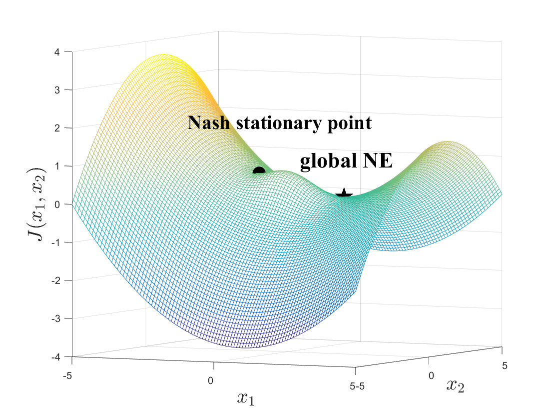
Figure 1: A non-convex two-player demo with log-sum-exp payoffs in (4).

Actually, as for convex games, most existing research computes global NE via investigating Nash stationary points [facchinei2010penalty, koshal2016distributed, chen2021distributed]. However, considering the bumpy geometric structure of the non-convex payoff function, one cannot expect to find a global NE of (1) merely via the Nash stationary conditions in (7). To this end, we aim at obtaining a global NE of such a non-convex multi-player model (1) and begin the exploration in the sequel.

4 Existence Condition of Global NE

In this section, we primarily explore the existence of global NE with the following procedures, that is,

1. We employ canonical duality theory to transform the original game (1) into a complementary dual problem, and investigate the relationship between the stationary points of the dual problem and the Nash stationary points of game (1);

2. We adopt a sufficient feasible domain for the introduced conjugate variable to investigate the global optimality of the stationary points;

3. We cast solving all players’ stationary point profile of the dual problem into solving a variational inequality (VI) problem with a continuous pseudo-gradient mapping;

4. We provide the existence condition of global NE of the non-convex multi-player game: the solution to the VI problem is required to satisfy a duality relation.

Step 1: Complementary dual problem

We first take $\xi_{i}=\Lambda_{i}(x_{i},\bm{x}_{-i})\in\Theta_{i}$ in the payoff function of (2), which is called a canonical measure. This follows the definition of canonical functions, for $i\in\mathcal{I}$. Since $\Psi_{i}(\xi_{i})$ is a convex canonical function, the one-to-one duality relation $\sigma_{i}=\nabla\Psi_{i}\left(\xi_{i}\right):\Theta_{i}\rightarrow\Theta^{*}_{i}$ implies the existence of the conjugate function $\Psi^{*}_{i}:\Theta^{*}_{i}\rightarrow\mathbb{R}$, which can be uniquely described by the Legendre transformation [rockafellar1974conjugate, 8770111, gao2017canonical], that is,

$$\Psi_{i}^{*}\left(\sigma_{i}\right)=\xi_{i}^{T}\sigma_{i}-\Psi_{i}\left(\xi_{i}\right),$$

where $\sigma_{i}\in\Theta_{i}^{*}$ is a canonical dual variable. Thus, denote $\bm{\sigma}=\operatorname{col}\{\sigma_{1},\cdots,\sigma_{N}\}$ and $\bm{\Theta}^{*}=\prod_{i=1}^{N}\Theta^{*}_{i}\subseteq\mathbb{R}^{q}$ with $q=\sum_{i=1}^{N}q_{i}$. Then the complementary function $\Gamma_{i}:\bm{\Omega}\times\Theta_{i}^{*}\rightarrow\mathbb{R}$ referring to the canonical duality theory can be defined as

$$\Gamma_{i}(x_{i},\sigma_{i},\bm{x}_{-i})= \xi_{i}^{T}\sigma_{i}-\Psi_{i}^{*}(\sigma_{i})$$

$$= \sigma_{i}^{T}\Lambda_{i}\left(x_{i},\bm{x}_{-i}\right)-\Psi_{i}^{*}\left(\sigma_{i}\right).$$ (8)

Lemma 1

There exists a profile $\bm{x}^{\Diamond}$ as a Nash stationary point of (1) if $\bm{\sigma}^{\Diamond}\in\bm{\Theta}^{*}$ and for $i\in\mathcal{I}$, $({x_{i}^{\Diamond}},{\sigma_{i}^{\Diamond}})$ is a stationary point of complementarity function $\Gamma_{i}(x_{i},\sigma_{i},\bm{x}_{-i}^{\Diamond})$.

Lemma 1 reveals the equivalency relationship of stationary points between (4) and (1). This means that we can close the duality gap between the non-convex original game and its canonical dual problem with the canonical transformation. More proof details of Lemma 1 can be found in the Supplementary Materials due to space limitations.

Step 2: Sufficient feasible domain

For $i\in\mathcal{I}$, we define the second-order partial derivative of $\Gamma_{i}(x_{i},{\sigma}_{i},\bm{x}_{-i})$ in $x_{i}$ is defined as follows.

$$P_{i}(\sigma_{i})=\nabla^{2}_{x_{i}}\Gamma_{i}=\sum\nolimits_{k=1}\nolimits^{q_{i}}[\sigma_{i}]_{k}\nabla^{2}_{x_{i}}\Lambda_{i,k}(x_{i},\bm{x}_{-i}).$$

Recalling that $\Lambda_{i}:\bm{\Omega}\rightarrow\Theta_{i}$ is a quadratic operator and $\nabla^{2}_{x_{i}}\Lambda_{i}$ is both $x_{i}$-free and $\bm{x_{-i}}$-free (see the cases in (3)-(5)), we can easily check that $P_{i}(\sigma_{i})$ is indeed a linear combination of $[\sigma_{i}]_{k}$. On this basis, we introduce the following set of $\sigma_{i}$ for $i\in\mathcal{I}$.

$$\mathscr{E}_{i}^{+}=\Theta_{i}^{*}\cap\{\sigma_{i}:P_{i}(\sigma_{i})\succeq\kappa_{x}\bm{I}_{n}\},$$ (9)

where the constant $\kappa_{x}>0$ and the further notation

$$\bm{\mathscr{E}}^{+}=\mathscr{E}_{1}^{+}\times\cdots\times\mathscr{E}_{N}^{+}.$$

When $\sigma_{i}\in\mathscr{E}_{i}^{+}$, the positive definiteness of $P_{i}(\sigma_{i})$ implies that $\Gamma_{i}(x_{i},{\sigma}_{i},\bm{x}_{-i})$ is convex with respect to $x_{i}$. Besides, the convexity of $\Psi_{i}(\xi_{i})$ derives that its Legendre conjugate $\Psi_{i}^{*}(\sigma_{i})$ is also convex. Hence, the complementary function $\Gamma_{i}(x_{i},{\sigma}_{i},\bm{x}_{-i})$ is concave in $\sigma_{i}$. This convex-concave property of $\Gamma_{i}$ enables us to further investigate the optimality of the stationary points of (4), that is, the optimality of the Nash stationary point of (1).

Remark 1

The computation of $\mathscr{E}_{i}^{+}$ is actually not so hard in most practical cases. For example, take the payoff function in (3) with $i=1,2$ and $n=q_{i}=1$. The complementary function is $\Gamma_{i}(x_{i},\sigma_{i},x_{3-i})=\sigma_{i}((x_{i}-x_{3-i})^{2}-d_{i,3-i})-\sigma_{i}^{2}/4$, where $x_{i}\in\Omega_{i}=[a,b]$ and $\sigma_{i}\in\Theta_{i}^{*}=[-2d_{i,3-i},2(b-a)^{2}-2d_{i,3-i}]$. Thus, the subset $\mathscr{E}_{i}^{+}=\left\{\sigma_{i}:2\sigma_{i}\geq\kappa_{x}\right\}\cap\Theta_{i}^{*}=[\kappa_{x}/2,2(b-a)^{2}-2d_{i,3-i}]$, which can serve as the feasible constraint set for the dual variable $\sigma_{i}$.

Step 3: Variational inequality

With the interference of $\bm{x}_{-i}$, the transformed problem actually reflects a cluster of $\Gamma_{i}$ with a mutual coupling of stationary conditions, rather than a deterministic one. Therefore, different from classic optimization works [zhu2012approximate, latorre2016canonical, gao2017canonical], the stationary points for player $i$ cannot be calculated independently. We should consider the computation of all players’ stationary point profile and discuss its optimality in an entire perspective.

To this end, variational inequalities (VI) help us to carry forward [facchinei2003finite]. Specifically, denote $\bm{z}=\operatorname{col}\{\bm{x},\bm{\sigma}\}$ and $\bm{\Xi}=\bm{\Omega}\times\mathscr{E}^{+}$. Take the following continuous mapping as the pseudo-gradient of (4).

$$F(\bm{z})=\operatorname{col}\Big{\{}\operatorname{col}\{\sum\nolimits_{k=1}\nolimits^{q_{i}}[\sigma_{i}]_{k}\nabla_{x_{i}}\Lambda_{i,k}(x_{i},\bm{x}_{-i})\} {}_{i=1}^{N},$$

$$\operatorname{col}\{-\Lambda_{i}(x_{i},\bm{x}_{-i})+\nabla\Psi_{i}^{*}(\sigma_{i})\} {}_{i=1}^{N}\Big{\}}.$$

Note that the interaction on all players’ variables is displayed in mapping $F$, which is a joint function of the partial derivatives of all players’ complementary functions (4). Then (4) can be cast as a VI problem $\operatorname{VI}(\bm{\Xi},F)$ to solve, i.e., finding $\bm{z}^{\Diamond}\in\bm{\Xi}$ such that

$$(\bm{z}-\bm{z}^{\Diamond})^{T}F(\bm{z}^{\Diamond})\geq 0,\quad\forall\bm{z}\in\bm{\Xi}.$$ (10)

Step 4: Existence condition

Based on the above steps, we have the following existence condition for identifying the global NE of (1).

Theorem 1

There exists $\bm{x}^{\Diamond}$ as the global NE of the non-convex multi-player game (1) if $(\bm{x}^{\Diamond},\bm{\sigma}^{\Diamond})$ is a solution to $\operatorname{VI}(\bm{\Xi},F)$ with $\sigma_{i}^{\Diamond}=\nabla\Psi_{i}\left(\xi_{i}\right)\mid_{\xi_{i}=\Lambda_{i}\left(x_{i}^{\Diamond},\bm{x}_{-i}^{\Diamond}\right)}$ for $i\in\mathcal{I}$.

The proof sketch can be summarized as below. Under Assumption 1, if there exists $\bm{\sigma}^{\Diamond}\in\mathscr{E}^{+}$ such that $\bm{z}^{\Diamond}=\operatorname{col}\{\bm{x}^{\Diamond},\bm{\sigma}^{\Diamond}\}$ is a solution to $\operatorname{VI}(\bm{\Xi},F)$, then it satisfies the first-order condition of the VI. Together with $\sigma_{i}^{\Diamond}=\nabla\Psi_{i}\left(\xi_{i}\right)\mid_{\xi_{i}=\Lambda_{i}\left(x_{i}^{\Diamond},\bm{x}_{-i}^{\Diamond}\right)}$, we claim that the canonical duality relation holds over $\Theta_{i}\times\mathscr{E}_{i}^{+}$ for $i\in\mathcal{I}$. It follows from Lemma 1 that the solution to $\operatorname{VI}(\bm{\Xi},F)$ is a stationary point profile of (4) on $\Theta_{i}\times\Theta_{i}^{*}$. We can further verify that the total complementary function $\Gamma_{i}(x_{i},\sigma_{i},\bm{x}_{-i})$ is concave in dual variable $\sigma_{i}$ and convex in $x_{i}$. In this light, we obtain the globally optimality of $(\bm{x}^{\Diamond},\bm{\sigma}^{\Diamond})$ on $\bm{\Omega}\times\mathscr{E}^{+}$, that is, for $x_{i}\in\Omega_{i}$ and $\sigma_{i}\in\mathscr{E}_{i}^{+}$,

$$\Gamma_{i}(x_{i}^{\Diamond},\sigma_{i},\bm{x}_{-i}^{\Diamond})\leq\Gamma_{i}(x_{i}^{\Diamond},\sigma_{i}^{\Diamond},\bm{x}_{-i}^{\Diamond})\leq\Gamma_{i}(x_{i},\sigma_{i}^{\Diamond},\bm{x}_{-i}^{\Diamond}).$$

This confirms that $\bm{x}^{\Diamond}$ is the global NE of (1). The whole proof of Theorem 1 can be found in the Supplementary Materials due to space limitations.

The result in Theorem 1 reveals that once the solution of $\operatorname{VI}(\bm{\Xi},F)$ is obtained, we can check whether the duality relation $\sigma_{i}^{\Diamond}=\nabla\Psi_{i}\left(\xi_{i}\right)\mid_{\xi_{i}=\Lambda_{i}\left(x_{i}^{\Diamond},\bm{x}_{-i}^{\Diamond}\right)}$ holds, so as to identify whether the solution of $\operatorname{VI}(\bm{\Xi},F)$ is a global NE. Based on the above conclusion, we are inspired to solve $\operatorname{VI}(\bm{\Xi},F)$ via its first-order conditions and employ the duality relation as a criterion for identifying the global NE.

Remark 2

The foundation to realize the above idea is the nonempty set $\mathscr{E}_{i}^{+}$. It is possible to obtain an empty $\mathscr{E}_{i}^{+}$ in reality, provided by $P_{i}(\sigma_{i})\succeq\kappa_{x}\bm{I}_{n}$ has no intersection with $\Theta_{i}^{*}$, and these situations make the above duality theory approach unavailable. Thus, $\mathscr{E}_{i}^{+}$ should be effectively checked once the problem is formulated. Such a process has also been similarly employed in some classic optimization works to solve non-convex problems [zhu2012approximate, liang2019topology, ren2021distributed, zheng2012zero, latorre2016canonical]. In addition, this is why we cannot directly employ the standard Lagrange multiplier method and the associated KKT theory, because we need to confirm a feasible d domain of multiplier $\sigma_{i}$ by utilizing canonical duality information (referring to $\Theta_{i}^{*}$).

Remark 3

By generalizing the coupled stationary conditions to continuous vector fields, we compactly formulate these stationary conditions of the dual problem (4) as a continuous mapping in a VI problem $\operatorname{VI}(\bm{\Xi},F)$. Thus, seeking all players’ stationary point profile (or Nash stationary point) can be accomplished by verifying a fixed point of this continuous mapping. The seed of employing the VI idea in game problems dates back to [harker1990finite], and has since found wide applications in various game models, for a survey, see [giannessi2006equilibrium] and the references therein.

5 Approaching Global NE via Conjugate-based ODE

In this section, we propose an ODE to seek the solutions to $\operatorname{VI}(\bm{\Xi},F)$ (10) with the assisted complementary information (the Legendre conjugate of $\Psi_{i}$ and the canonical dual variable $\sigma_{i}$). In fact, an ODE provides continuously evolved dynamics, which help reveal how the primal variables and the canonical dual ones influence each other via conjugate gradient information. Meanwhile, the analysis techniques in modern calculus and nonlinear systems for theoretical guarantees of ODEs may lead to comprehensive results with mild assumptions.

5.1 ODE Design

Consider that the local set constraints of variables, like $\Omega_{i}$ and $\mathscr{E}_{i}^{+}$ of (10), are usually equipped with specific structures in various tasks. We intend to employ conjugate properties of the generating functions within Bregman divergence to design ODE flows. Take $\phi_{i}(x_{i})$ and $\varphi_{i}(\sigma_{i})$ as two generating functions, where $\phi_{i}(x_{i})$ is $\mu_{x}$-strongly convex and $L_{x}$-smooth on $\Omega_{i}$, and $\varphi_{i}(\sigma_{i})$ is $\mu_{\sigma}$-strongly convex and $L_{\sigma}$-smooth on $\mathscr{E}_{i}^{+}$. It follows from the Fenchel inequality [diakonikolas2019approximate] that the Legendre conjugate $\phi_{i}^{*}$ and $\varphi_{i}^{*}$ are convex and differentiable, where for $y_{i}\in\mathbb{R}^{n}$,

$$\phi_{i}^{*}(y_{i})\triangleq\operatorname{min}_{x_{i}\in\Omega_{i}}\{-x_{i}^{T}y_{i}+\phi_{i}(x_{i})\},$$

and for $\nu_{i}\in\mathbb{R}^{q_{i}}$,

$$\varphi_{i}^{*}(\nu_{i})\triangleq\operatorname{min}_{\sigma_{i}\in\mathscr{E}_{i}^{+}}\{-\sigma_{i}^{T}\nu_{i}+\varphi_{i}(\sigma_{i})\}.$$

Accordingly, their conjugate gradients satisfy

$$\nabla\phi_{i}^{*}(y_{i})=\operatorname{argmin}_{x_{i}\in\Omega_{i}}\left\{-x_{i}^{T}y_{i}+\phi_{i}(x_{i})\right\},$$ (11)

$$\nabla\varphi_{i}^{*}(\nu_{i})=\operatorname{argmin}_{\sigma_{i}\in\mathscr{E}_{i}^{+}}\{-\sigma_{i}^{T}\nu_{i}+\varphi_{i}(\sigma_{i})\}.$$ (12)

TABLE I: Closed-form conjugate gradients with different generating functions.

	Feasible set	Generating function	Conjugate gradient
General convex set	$\Omega$	$\!\frac{1}{2}\|x\|^{2}_{2}$	$\!{\operatorname{argmin}_{x\in\Omega}}\frac{1}{2}\|x\!-\!y\|^{2}$
Non-negative orthant	$\mathbb{R}^{n}_{+}$	$\!\!\sum\nolimits_{l=1}\nolimits^{n}\!x^{l}\log(x^{l})\!-\!x^{l}$	${\exp(y)}$
Unit square $[a,b]^{n}$	$\!\!\{x^{l}\!\in\!\mathbb{R}\!\!:\!a\!\leq\!x^{l}\!\leq\!b\}$		col{a+bexp(yl)exp(yl)+1}l=1n
SimplexΔn	​​{x​∈​Rn+​:​∑nl=1​xl=1}	​∑l=1n​xllog(xl)	col{exp(yl)∑j=1nexp(yj)}l=1n
EuclideansphereBnρ(w)	​​{