Towards Rigorous Understanding of Neural Networks via Semantics-preserving Transformations

Abstract

In this paper, we present an algebraic approach to the precise and global verification and explanation of Rectifier Neural Networks, a subclass of Piece-wise Linear Neural Networks (PLNNs), i.e., networks that semantically represent piece-wise affine functions. Key to our approach is the symbolic execution of these networks that allows the construction of semantically equivalent Typed Affine Decision Structures (TADS). Due to their deterministic and sequential nature, TADS can, similarly to decision trees, be considered as white-box models and therefore as precise solutions to the model and outcome explanation problem. TADS are linear algebras, which allows one to elegantly compare Rectifier Networks for equivalence or similarity, both with precise diagnostic information in case of failure, and to characterize their classification potential by precisely characterizing the set of inputs that are specifically classified, or the set of inputs where two network-based classifiers differ. All phenomena are illustrated along a detailed discussion of a minimal, illustrative example: the continuous XOR function.

1 Introduction

Neural networks are perhaps today’s most important machine learning models, with exciting results, e.g., in image recognition [SZ14], speech recognition [CSW⁺18, BMR⁺20] and even in highly complex games [VBC⁺19, BBC⁺19, SSS⁺17]. As the name suggests, neural networks are learned from data using efficient, but approximate training algorithms [Rud16, KB14]. At their core, neural networks are (dataflow-oriented) computation graphs [GBC16]. They consist of many computation units, called neurons, that are arranged in layers such that computations in each layer can be performed in parallel, with successive layers only depending on the preceding layer. Modern neural networks, in practice, possess up to multiple billions of parameters [BMR⁺20] and leverage parallel hardware such as GPUs to perform computations of this scale [OJ04]. This highly quantitative approach is responsible for exciting success stories, but also for their main weakness: Neural network behavior is often chaotic and hard to comprehend for a human. Perhaps most infamously, a neural network’s prediction can change drastically under imperceptible changes to its input, so-called adversarial examples [MMS⁺17, GSS14, SZS⁺13].

The explainability of neural networks, which are computationally considered as black-boxes due to their highly parallel and non-linear nature, is therefore one of the current core challenges in AI research [DSB17]. The fact that neural networks are increasingly used in safety-critical systems such as self-driving cars [BGC⁺21] turns trustworthiness of machine learning into a must [DSB17]. However, state-of-the-art explanation technology is more about reassuring intuition, e.g., to support cooperative work of humans with AI systems, such as in the field of medical diagnostics [TG20], than about precise explanation or guarantees [LPK21]. Moreover, current approaches to Neural Network verification are still in their infancy in that they are not yet sufficiently tailored to the nature of Neural Networks to achieve the required scalability or to provide diagnostic information beyond individual witness traces in cases where the verification attempts fail (cf., [BLJ21, KBD⁺17, WZX⁺21] and Section 8 for a more detailed discussion).

In this paper, we present an algebraic approach to the verification and explanation of Rectifier Neural Networks (PLNN), a very popular subclass of neural networks that semantically represent piece-wise affine functions (PAF) [MPCB14]. Key to our approach are Typed Affine Decision Structures (TADS) that concisely represent PAF in a white-box fashion that is as accessible to human understanding as decision trees. TADS can nicely be derived from PLNNs via symbolic execution [Cla76, Kin76], or, alternatively, compositionally along the PLNN’s layering structure, and their algebraic structure allows for elegant solutions to verification and explanation tasks:

• TADS can be used for PLNNs similarly as Algebraic Decision Diagrams (ADDs) have been used for Random Forests in [GS21] to elegantly provide model and outcome explanations as well as class characterizations.

• Using the algebraic operations of TADS one can not only decide the equivalence problem, i.e., whether two PLNNs are semantically equivalent, but also whether they are $\epsilon$-similar, i.e., never differ more than $\epsilon$. In both cases, diagnostic information in terms of a corresponding ‘difference’ TADS is provided that precisely specifies where one of these properties is violated.

• TADS comprise non-continuous piece-wise linear operations which cannot be represented by PLNNs. This is necessary to not only deal with regression tasks, where one aims at approximating continuous functions, but also with classification tasks with discrete output domains. In the latter case, TADS-based class characterization allows one to precisely characterize the set of inputs that are classified as members of a given class, or the set of inputs where two (PLNN-based) classifiers differ.

• Finally, TADS can also profitably be used for the verification of preconditions and postconditions, the illustration of which is beyond the scope of this paper, but will be discussed in [NSMB23] in the setting of digit recognition.

The paper illustrates the essential features of TADS using a minimal, illustrative example: the continuous XOR function. The simplicity of XOR is ideally suited to provide an intuitive entry into the presented theory. A more comprehensive example is presented in [NSMB23], where digit recognition based on the MNIST data base is considered. In this highly dimensional setting, specific scalability measures are required to apply our TADS technology.

After specifying the details of our running example in Section 2, Section 3 sketches Algebraic Decision Structures that later on will be instantiated with Affine Functions recalled in Section 4 to introduce the central notion of this paper, Typed Affine Decision Structures (TADS). Semantically, TADS represent piece-wise affine functions, which marks them as a fitting representation for Rectifier Networks that represent continuous piece-wise affine functions and that are discussed in Section 5. Our main contribution is the derivation of TADS, using both symbolic execution and compositionality along the layering structure of PLNN, as a complete and precise model explanation of PLNNs. We introduce TADS in Section 6 and state important algebraic properties that allow the manipulations mentioned beforehand. Subsequently, Section 7 illustrates the impact on verification and explanation of the algebraic properties of TADS that are also established in Section 6 along the running example. The paper closes after a discussion of related work in Section 8 with conclusions and direction to future work in Section 9.

2 Running Example – XOR

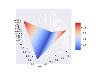
Figure 1: A baseline solution to the XOR-regression problem given by $f_{*}(x,y)=|x-y|$. Note that this function is piece-wise linear, having two separate linear regions, which is minimal for the problem.

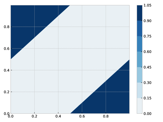
Figure 2: A baseline solution to the XOR-classification problem given by $g_{*}(x,y)=1$ iff $f_{*}(x,y)\geq 0.5$.

As a running example throughout this paper, we discuss the XOR function under the perspective of a regression task and a classification task, as specified below. We chose the XOR problem for illustration for two reasons:

• The XOR problem concerns a two-dimensional function which can be visualized as a function plot.

• While simple, the XOR problem has been a roadblock in early AI research because it cannot be solved by linear approaches [MP69]. Therefore, it is a minimal problem that still requires a more powerful non-linear model such as a PLNN.

For the following formalizations, let us fix some basic notation: The set of natural numbers (including zero) is denoted $\mathbb{N}$ and the set of real numbers $\mathbb{R}$. Unions and intersections of sets are defined as usual. The cartesian product of two sets is defined as

$$M\times N\mathrel{\vcentcolon=}\{\,(x,y)\nonscript\>|\allowbreak\nonscript\>\mathopen{}x\in M\>\land\>y\in N\,\}.$$

A sequence of cartesian products over the same set may be abbreviated as $M^{n}$ ($n\geq 0$), where

$$M^{0} =\emptyset M^{1} =M M^{n+2} =M\times M^{n+1}$$

and the Kleene star operator is defined as

$$M^{*}\mathrel{\vcentcolon=}\bigcup_{n\in\mathbb{N}}M^{n}$$

Moreover, intervals of $\mathbb{R}$ are of the form $[a,b]$ for $a,b\in\mathbb{R}$ with $a\leq b$ and denote the set of all real values between $a$ and $b$.

As a regression task, the XOR problem is stated as follows:

Definition 2.1 (XOR Regression).

Find a piece-wise affine function $f\colon[0,1]^{2}\rightarrow[0,1]$ that is continuous and satisfies:

$$f(0,0)\approx 0\approx f(1,1)\quad\text{and}\quad f(1,0)\approx 1\approx f(0,1)$$

Thus, a learning algorithm is tasked with approximating a continuous version of an XOR gate, interpolating between the four edge points for which the XOR function is defined.

When posing the XOR problem as a classification task, the XOR function can be regarded as a function with discrete binary output $1$ or $0$ but with a continuous domain $\mathbb{R}^{2}$.

Definition 2.2 (XOR Classification).

Find a piece-wise affine function $f\colon[0,1]^{2}\rightarrow\{0,1\}$ such that:

$$f(0,0)=0=f(1,1)\quad\text{and}\quad f(1,0)=1=f(0,1)$$

As the XOR-problem requires fixed values only at four points, there exist infinitely many solutions. This is typical for machine learning problems where only some few points are fixed and others are left for the machine learning model to freely interpolate. Different machine learning models have different principles that dictate this interpolation. For example, concerning PLNNs, the interpolation is (piece-wise) linear.

In line with the principle of Occam’s razor [Sob15], humans would optimally solve the XOR-regression problem with a function as simple as:

$$f_{*}(x,y)=\lvert x-y\rvert$$

A visualisation of $f_{*}$ can be found in Figure 1. Similarly, a human would probably choose the following corresponding straightforward extension to the classification problem:

$$g_{*}(x,y)=\begin{cases}1\quad&\text{if }f_{*}(x,y)\geq 0.5\\ 0\quad&\text{otherwise}\end{cases}$$

An illustration of $g_{*}$ can be found in Figure 2. It is straightforward to check that these functions solve the XOR-regression and XOR-classification problems optimally in the sense that they match the traditional XOR function at all points where it is defined.

The continuous XOR problems will serve as running examples throughout this work: We will demonstrate different representations of piece-wise linear functions (such as $f_{*}$) and transformations between them along the development of our theory, and showcase differences between the manually constructed solutions to the regression and classification tasks and their learned counterparts in Section 7.

3 Algebraic Decision Structures

In order to prepare the algebraic treatment of decision structures, we focus on decision structures whose leafs are labeled with the elements of an algebra $A=(\mathcal{A},O)$, so-called Algebraic Decision Structures (ADDs). This subsumes the classical case where leafs of decision structures are elements of a set, as these are simply algebras where $O$ is empty. In this section we summarize the definitions and theorems of [GS21], which are required later in this paper.

Definition 3.1 (Algebraic Structures).

An algebraic structure, or algebra for short, is a pair $(\mathcal{A},O)$ of a carrier set $\mathcal{A}$ and a set of operations $O$. Operations $\mathit{op}\in O$ have a fixed arity and are closed under $\mathcal{A}$.

In the following, the algebra is identified with its carrier set and both are written calligraphically.

Definition 3.2 (Algebraic Decision Tree).

An Algebraic Decision Tree (ADT) over the algebra $A$ and the predicates $\mathcal{P}$ is inductively defined by the following BNF:

$$T\>\mathrel{\vcentcolon\vcentcolon=}\>\varepsilon\,\mathbin{|}\,a\,\mathbin{|}\,(p,T,T)\quad\textrm{ with }a\in\mathcal{A}\textrm{ and }p\in\mathcal{P}\textrm{.}$$

ADTs are (directed) trees where for a node $(p,l,r)$ the root is given by $p$ and the left and right children by $l$ and $r$, respectively. ADTs of the form $a$ are leafs with no children and $\varepsilon$ denotes the empty tree. We can merge nodes in these ADTs, which leads to the more general Algebraic Decision Structures (ADS):

Definition 3.3 (Node Merging).

Let $t$ be an ADT and $t_{1}$ and $t_{2}$ be two nodes in $t$ such that $t_{2}$ is not reachable from $t_{1}$. Then, the two-step transformation of $t$

• re-route the incoming edges of $t_{2}$ to $t_{1}$ and

• eliminate all unreachable nodes of $t$.

is called a $t_{2}$ into $t_{1}$ merge.

Node merges aggregate subtrees in a manner that does not create directed cycles. Later, we will define semantics preserving merges.

Definition 3.4 (Algebraic Decision Structure).

A rooted directed acyclic graph (DAG) that results from an ADT by a series of node merges is called an Algebraic Decision Structure (ADS). Let $\mathcal{S}_{\scriptsize A}$ denote the set of all such ADSs over an algebra $A$.

We can define their semantics inductively.

Definition 3.5 (Decision Structure Semantics).

For a set $\Sigma$ of valuations the semantic function

$$\llbracket\,\cdot\,\rrbracket_{\scriptscriptstyle\mathcal{S}\!_{A}}:\mathcal{S}_{\scriptsize A}\rightarrow(\Sigma\rightarrow\mathcal{A})$$

for ADSs is inductively defined as

$$\llbracket a\rrbracket_{\scriptscriptstyle\mathcal{S}\!_{A}}(\sigma) \mathrel{\vcentcolon=}a$$

$$\llbracket(p,l,r)\rrbracket_{\scriptscriptstyle\mathcal{S}\!_{A}}(\sigma) \mathrel{\vcentcolon=}\begin{cases}\llbracket l\rrbracket_{\scriptscriptstyle\mathcal{S}\!_{A}}(\sigma)&\textrm{if }\llbracket p\rrbracket(\sigma)=1\\ \llbracket r\rrbracket_{\scriptscriptstyle\mathcal{S}\!_{A}}(\sigma)&\textrm{if }\llbracket p\rrbracket(\sigma)=0\end{cases}$$

ADS can be considered the universe in which we operate, typically using semantics-preserving transformations. In particular, we will frequently apply semantic reduction and infeasible path reduction as discussed in the next two subsections. These two operations reduce the representational overhead of ADS while preserving their semantics.

3.1 Semantic Reduction

Semantic functions naturally induce an equivalence relation:

Definition 3.6 (Semantic Equivalence).

Two ADSs $t_{1}$ and $t_{2}$ are semantically equivalent iff their semantic functions coincide

$$t_{1}\sim t_{2}\quad\textrm{iff}\quad\llbracket t_{1}\rrbracket_{\scriptscriptstyle\mathcal{S}\!_{A}}=\llbracket t_{2}\rrbracket_{\scriptscriptstyle\mathcal{S}\!_{A}}$$

The following theorem states that one of two different nodes of an ADS that are semantically equivalent is redundant:

Theorem 3.7 (Semantic Reduction).

Let $t$ be an ADS with two nodes $t_{1}$ and $t_{2}$ that are semantically equivalent, i.e., $t_{1}\sim t_{2}$, and such that $t_{2}$ is not reachable from $t_{1}$. Moreover, let $t_{3}$ be the $t_{2}$ into $t_{1}$ merge of $t$. Then $t$ and $t_{3}$ are semantically equivalent, i.e., $t\sim t_{3}$.

Our implementation heuristically reduces the number of semantically equivalent nodes of the ADSs. However, in contrast to Algebraic Decision Diagrams [BFG⁺97], which are known for their normal forms, we cannot guarantee canonicity here.

3.2 Vacuity Reduction

Typically, there are dependencies between different predicates in $\mathcal{P}$, which induces so-called infeasible paths in the corresponding ADSs. This can be exploited for further reducing ADSs by eliminating so-called vacuous predicates:

Definition 3.8 (Vacuity).

Let $\bar{\mathcal{P}}$ be the set of negated predicates of $\mathcal{P}$. Then we call $\pi=p_{0}\cdots p_{m}\in(\mathcal{P}\cup\bar{\mathcal{P}})^{*}$ a predicate path.

• $\pi$ is called a predicate path of a decision structure $t\in\mathcal{S}_{\scriptsize A}$ iff there exists a path $\pi^{\prime}=p^{\prime}_{0}\cdots p^{\prime}_{m}\in\mathcal{P}^{*}$ from the root of $t$ to one of its other nodes such that $p_{i}=p^{\prime}_{i}$ in case that $\pi^{\prime}$ follows the left/true branch at $p_{i}$ in $t$ and $p_{i}=\bar{p}^{\prime}_{i}$ otherwise.

  We denote the last predicate $p_{m}\in\mathcal{P}\cup\bar{\mathcal{P}}$ of $\pi$ by $\mathit{final}(\pi)$.

• Given a predicate path $\pi=p_{0}\cdots p_{m}$ the predicate $\mathit{final}(\pi)$ is called vacuous for $\pi$ iff the conjunction of the preceding predicates $p_{0}\land\cdots\land p_{m-1}$ in $\pi$ implies $\mathit{final}(\pi)$.

• Let $\Pi_{n}$ be the set of predicate paths of $t\in\mathcal{S}_{\scriptsize A}$ that end in a given node $n$. We call $n$ vacuous in $t$, iff $\mathit{final}(\pi)$ is vacuous for all paths $\pi\in\Pi$ and $\mathit{final}(\pi)$ coincides for all $\pi$.

• A decision structure $t\in\mathcal{S}_{\scriptsize A}$ is called vacuity-free iff there exists no vacuous node.

This allows us to define the following optimization step.

Definition 3.9 (Vacuity Reduction).

Let $t\in\mathcal{S}_{\scriptsize A}$ be a decision structure with a vacuous node $n$ and $\mathit{final}(\pi)\in\mathcal{P}\cup\bar{\mathcal{P}}$ be the last predicate of some predicate path $\pi$ ending in $n$. Then, re-routing all incoming edges of $n$ to the ’true’-successor of $n$ in case of $\mathit{final}(\pi)\in\mathcal{P}$ and to the ’false’-successor otherwise is called a vacuity reduction step.

ADSs, being DAGs, only have finitely many predicate paths which can be effectively analysed for vacuous predicates, as long as the individual predicates are decidable. As the elimination of vacuous predicates is a simple semantics-preserving transformation, we have:

Theorem 3.10 (Minimality).

Every ADS can be effectively transformed into a semantically equivalent, vacuity-free ADS that is minimal in the sense that any further reduction would change its semantics.

In the remainder of the paper, we will not explicitly discuss the effects of semantic reduction and vacuity reduction. Rather, we will concentrate on the algebraic properties of ADS that they inherit from their leaf algebra via lifting.

3.3 Lifting

It is well-known that algebraic structures $A=(\mathcal{A},O)$ can point-wise be lifted to cartesian products and arbitrary function spaces $M\to A$. This has successfully been exploited for Binary Decision Diagrams (BDDs) and Algebraic Decision Diagrams (ADDs) that canonically represent functions of type $\mathbb{B}^{n}\to\mathbb{B}$ and $\mathbb{B}^{n}\to\mathcal{A}$ respectively. In fact, the canonicity of these representations allows one to identify the BDD/ADD representations directly with their semantics, which in particular reduces the verification of semantic equivalence to checking for isomorphism.

In our case, canonicity is unrealistic for two reasons (cf., Section 6.1):

1. Considering predicates rather than Boolean values introduces infeasibility and thereby prohibits minimal canonical representations.

2. The ordering of predicates may lead to an exponential explosion of the representation. Please note that, in contrast to, e.g., the typical BDD setting, we do not have just a few (64, 128, 256,$\ldots$ or the like) input bits that specify the control of some circuit, but predicates capture the effect of the ReLU function in a history-dependent way; Predicates that result from computations in a later layer depend on predicates from earlier layers. Moreover, as predicates are continuous objects, the probability of them coinciding can be considered $0$. Thus, ordering predicates would typically lead to representations that are doubly exponential in the number of neurons of a neural network.

We will see, however, that all the algebraic properties we need also hold for unordered ADSs, and that we can conveniently compute on (arbitrary) representatives of the partition defined by semantic equivalence. This way, we arrive at an exponential worst-case complexity (in the size of the argument PLNNs) both, for the algebraic operations and the decision of semantic equivalence.

Although ADSs are not canonical one can effectively apply operators on concrete representatives while preserving semantics. Every operator can be lifted inductively as follows

Definition 3.11 (Lifted Operators).

For every operator $\mathbin{\scalerel*{\square}{\diamond}}:\mathcal{A}^{2}\to\mathcal{A}$ of an algebra $A=(\mathcal{A},O)$ we define the lifted operator $\mathbin{\scalerel*{\blacksquare}{\diamond}}\colon\mathcal{S}_{\scriptsize A}{}^{2}\to\mathcal{S}_{\scriptsize A}$ that operates over ADS inductively as

$$a\mathbin{\scalerel*{\blacksquare}{\diamond}}a^{\prime} =a\mathbin{\scalerel*{\square}{\diamond}}a^{\prime}$$

$$a\mathbin{\scalerel*{\blacksquare}{\diamond}}(p,l,r) =(p,a\mathbin{\scalerel*{\blacksquare}{\diamond}}l,a\mathbin{\scalerel*{\blacksquare}{\diamond}}r)$$

$$(p,l,r)\mathbin{\scalerel*{\blacksquare}{\diamond}}t =(p,l\mathbin{\scalerel*{\blacksquare}{\diamond}}t,r\mathbin{\scalerel*{\blacksquare}{\diamond}}t)$$

where $a,a^{\prime}\in\mathcal{A}$ are ADS identified with an element of the algebra, $t,l,r\in\mathcal{S}_{\scriptsize A}$ are ADS, and $p\in\mathcal{P}$ is a predicate.

Intuitively, for two ADS $t_{1}$ and $t_{2}$, this construction replaces leaves in $t_{1}$ with copies of $t_{2}$. Thus, each path of the resulting ADS $t_{3}$ expresses a conjunction of one path in $t_{1}$ and one path in $t_{2}$. The partition of the domain imposed by all paths of $t_{2}$ therefore coincides with the intersection imposed by the intersection of partitions imposed by $t_{1}$ and $t_{2}$. The required lifting of the operators to leaf nodes is straightforward (cf., Figure 4 for illustration).

The following theorem which states the correctness of the lifted operators can straightforwardly be proved by induction:

Theorem 3.12 (Correctness of Lifted Operators).

Let $t_{1},t_{2}\in\mathcal{S}_{\scriptsize A}$ be two ADS over some algebra ${A=(\mathcal{A},O)}$. Let $\mathbin{\scalerel*{\blacksquare}{\diamond}}\colon\mathcal{S}_{\scriptsize A}{}^{2}\to\mathcal{S}_{\scriptsize A}$ denote the lifted version of the operator $\mathbin{\scalerel*{\square}{\diamond}}\in O$. Then the following equation holds for all $\sigma\in\Sigma$:

$$\llbracket t_{1}\mathbin{\scalerel*{\blacksquare}{\diamond}}t_{2}\rrbracket_{\scriptscriptstyle\mathcal{S}\!_{A}}(\sigma)\mathrel{\vcentcolon=}\llbracket t_{1}\rrbracket_{\scriptscriptstyle\mathcal{S}\!_{A}}(\sigma)\mathbin{\scalerel*{\square}{\diamond}}\llbracket t_{2}\rrbracket_{\scriptscriptstyle\mathcal{S}\!_{A}}(\sigma)$$

3.4 Abstraction

Abstraction is one of the most powerful means for achieving scalability. The following easy to prove theorem concerns the interplay of abstractions imposed by a homomorphism of the leaf algebra and their effect on some classification function.

Theorem 3.13 (Abstraction).

Let $A=(\mathcal{A},O)$ and $A^{\prime}=(\mathcal{A^{\prime}},O^{\prime})$ be two algebras, and $\alpha\colon A\rightarrow A^{\prime}$ a homomorphism. Then $\alpha_{S}\colon\mathcal{S}_{\scriptsize A}\rightarrow\mathcal{S}_{\scriptsize A^{\prime}}$ defined by simply applying $\alpha$ to all the leaves of the argument ADS completes the following commutative diagram:

We will see in Section 7 how elegantly abstraction can be dealt with in the TADS setting: The abstraction that transforms the XOR regression setting into a classification setting can be easily realized via the TADS composition operator.

4 Affine Functions

The following notations of linear algebra are based on the book [Axl97]. The real vector space $(\mathbb{R}^{n},+,\cdot)$ with $n>0$ is an algebraic structure with the operations

$$+ \colon\mathbb{R}^{n}\times\mathbb{R}^{n}\to\mathbb{R}^{n}$$ vector addition

$${}\cdot{} \colon\mathbb{R}\phantom{{}^{n}}\times\mathbb{R}^{n}\to\mathbb{R}^{n}$$ scalar multiplication

which are defined as

$$(x_{1},\dots,x_{n})+(y_{1},\dots,y_{n}) =(x_{1}+y_{1},\dots,x_{n}+y_{n})$$

$$\lambda\cdot(x_{1},\dots,x_{n}) =(\lambda\cdot x_{1},\dots,\lambda\cdot x_{n})$$

A real vector $(x_{1},\dots,x_{n})$ of $\mathbb{R}^{n}$ is abbreviated as $\vec{x}$. To refer to one of the components, we write $\vec{x}_{i}\mathrel{\vcentcolon=}x_{i}$ (note the arrow ends before the subscript in contrast to $\vec{x_{i}}$, which denotes the $i$-th vector). The dimension of a real vector space $\mathbb{R}^{n}$ is given as $\dim\mathbb{R}^{n}=n$.

A matrix $\bm{W}$ is a collection of real values arranged in a rectangular array with $n$ rows and $m$ columns.

$$\bm{W}=\begin{pmatrix}w_{1,1}&w_{1,2}&\dots&w_{1,m}\\ w_{2,1}&w_{2,2}&\dots&w_{2,m}\\ \vdots&\vdots&\ddots&\vdots\\ w_{n,1}&w_{n,2}&\dots&w_{n,m}\end{pmatrix}$$

To indicate the number of rows and columns, one says $\bm{W}$ has type $n\times m$ also notated as $\bm{W}\in\mathbb{R}^{n\times m}$.

An element at position $i,j$ of the matrix $\bm{W}$ is denoted by $\bm{W}_{i,j}\mathrel{\vcentcolon=}w_{i,j}$ (where $1\leq i\leq n$ and $1\leq j\leq m$). A matrix $\bm{W}\in\mathbb{R}^{n\times m}$ can be reflected along the main diagonal resulting in the transpose $\bm{W}^{\transp}$ of shape $m\times n$ defined by the equation

$$\big{(}\>\bm{W}^{\transp}\>\big{)}_{i,j}\mathrel{\vcentcolon=}\bm{W}_{j,i}$$

The $i$-th row of $\bm{W}$ can be regarded as a $1\times m$ matrix given by

$$\bm{W}_{i,\cdot}\mathrel{\vcentcolon=}(w_{i,1},\dots,w_{i,m}).$$

Similarly, the $j$-th column of $\bm{W}$ can be regarded as a $n\times 1$ matrix defined as

$$\bm{W}_{\cdot,j}\mathrel{\vcentcolon=}(w_{1,j},\dots,w_{n,j})^{\transp}.$$

Matrix addition is defined over matrices with the same type to be component-wise, i.e.,

$$\big{(}\>\bm{W}+\bm{N}\>\big{)}_{i,j}\mathrel{\vcentcolon=}\bm{W}_{i,j}+\bm{N}_{i,j}$$

and scalar multiplication as

$$\big{(}\>\lambda\cdot\bm{W}\>\big{)}_{i,j}\mathrel{\vcentcolon=}\lambda\cdot\bm{W}_{i,j}.$$

The (type-correct) multiplication of two matrices ${\bm{W}\in\mathbb{R}^{n\times r}}$ and $\bm{N}\in\mathbb{R}^{r\times m}$ is defined as

$$\big{(}\>\bm{W}\cdot\bm{N}\>\big{)}_{i,j}\mathrel{\vcentcolon=}\sum_{k=1}^{r}\bm{W}_{i,k}\cdot\bm{N}_{k,j}$$

Identifying

• $n\times 1$ matrices with (column) vectors

• $1\times m$ matrices with row vectors

• $1\times 1$ matrices with scalars

as indicated above, makes the well-known dot product of $\vec{v},\vec{w}\in\mathbb{R}^{n}$

$${{\vec{v}}^{\top}\!}\cdot{\vec{w}}\mathrel{\vcentcolon=}\sum_{i=1}^{n}\vec{v}_{i}\cdot\vec{w}_{i}$$

just a special case of matrix multiplication. The same holds for matrix-vector multiplication that is defined for a $n\times m$ matrix $\bm{W}$ and a vector $\vec{x}\in\mathbb{R}^{n}$ as

$$\big{(}\>\bm{W}\cdot\vec{x}\>\big{)}_{i}\mathrel{\vcentcolon=}\bm{W}_{i,\cdot}\cdot\vec{x}$$

Matrices with the same number of rows and columns, i.e., with type $n\times n$ for some $n\in\mathbb{N}$, are said to be square matrices. Square matrices have a neutral element for matrix multiplication, called identity matrix, that is zero everywhere except for the entries on the main diagonal which are one.

$$\bm{I}^{n}\mathrel{\vcentcolon=}\begin{pmatrix}1&&0\\ &\ddots&\\ 0&&1\\ \end{pmatrix}$$

The $i$-th unit vector $\vec{\mathrm{e}_{i}}$ is a vector where all entries are zero except the $i$-th which is one.

4.1 Piece-wise Affine Functions

Definition 4.1 (Affine Function).

A function $\alpha\colon\mathbb{R}^{n}\rightarrow\mathbb{R}^{m}$ is called affine iff it can be written as

$$\alpha(\vec{x})=\bm{W}\vec{x}+\vec{b}$$

for some matrix $\bm{W}\in\mathbb{R}^{m\times n}$ and vector $b\in\mathbb{R}^{m}$.

We identify the semantics and syntax of affine functions with the pair $(\bm{W},\vec{b})$, which can be considered as a canonical representation of affine functions. Furthermore, we denote the set of all affine functions $\mathbb{R}^{n}\rightarrow\mathbb{R}^{m}$ as $\Phi(n,m)$ and call $(n,m)$ the type of $\Phi(n,m)$. The untyped version $\Phi$ is meant to refer to the set of all affine functions, independently of their type.

Lemma 4.2 (Operations on Affine Functions).

Let $\alpha_{1},\alpha_{2}$ be two affine functions in canonical form, i.e.,

$$\alpha_{1}(\vec{x}) =\bm{W_{1}}\vec{x}+\vec{b_{1}}$$

$$\alpha_{2}(\vec{x}) =\bm{W_{2}}\vec{x}+\vec{b_{2}}$$

Assuming matching types, the operations $+$ (addition), $\cdot$ (scalar multiplication), and $\circ$ (function application) can be calculated on the representation as

$$(s\cdot\alpha_{1})(\vec{x}) =(s\cdot\bm{W_{1}})\,\vec{x}+(s\cdot\vec{b_{1}})$$

$$(\alpha_{1}+\alpha_{2})(\vec{x}) =(\bm{W_{1}}+\bm{W_{2}})\,\vec{x}+(\vec{b_{1}}+\vec{b_{2}})$$

$$(\alpha_{2}\circ\alpha_{1})(\vec{x}) =(\bm{W_{2}}\bm{W_{1}})\,\vec{x}+(\bm{W_{2}}\vec{b_{1}}+\vec{b_{2}})$$

resulting again in an affine function in canonical representation.

It is well-known that the type resulting from function composition evolves as follows

$$\circ\colon\Phi(r,m)\times\Phi(n,r)\to\Phi(n,m).$$

The type of the operation is important for the closure axiom, the basis for most algebraic structures. This leads to the following well-known theorem [Axl97]:

Theorem 4.3 (Algebraic Properties).

Denoting, as usual, scalar multiplication with $\cdot$ and function composition with $\circ$, we have:

• $(\Phi(n,m),+,\cdot)$ forms a vector space and

• $(\Phi(n,n),\circ)$ forms a monoid.

This theorem can straightforwardly be lifted to untyped $\Phi$ by simply restricting all operations to the cases where they are well-typed, i.e., where addition is restricted to functions of the same type ($+_{t}$), and function composition to situation where the output type of the first function matches the input type of the second ($\circ_{t}$):

Theorem 4.4 (Properties of Typed Operations).

The quadruple $(\Phi,+_{t},\cdot,\circ_{t})$ forms a typed algebra, i.e., an algebraic structure that is closed under well-typed operations.

Piece-wise affine functions are usually defined over a polyhedral partitioning of the pre-image space [Bro83, GZB94, Ovc10].

Definition 4.5 (Halfspace).

Let $\vec{w}\in\mathbb{R}^{n}$ and $b\in\mathbb{R}$. Then the set

$$p=\{\,\vec{x}\in\mathbb{R}^{n}\nonscript\>|\allowbreak\nonscript\>\mathopen{}{{\vec{w}}^{\top}\!}\cdot{\vec{x}}+b=0\,\}$$

is called a hyperplane of $\mathbb{R}^{n}$. A hyperplane partitions $\mathbb{R}^{n}$ into two convex subspaces, called halfspaces. The positive and negative halfspaces of $p$ are defined as

$$p^{+} \mathrel{\vcentcolon=}\{\,\vec{x}\in\mathbb{R}^{n}\nonscript\>|\allowbreak\nonscript\>\mathopen{}{{\vec{w}}^{\top}\!}\cdot{\vec{x}}+b>0\,\}$$

$$p^{-} \mathrel{\vcentcolon=}\{\,\vec{x}\in\mathbb{R}^{n}\nonscript\>|\allowbreak\nonscript\>\mathopen{}{{\vec{w}}^{\top}\!}\cdot{\vec{x}}+b<0\,\}$$

Definition 4.6 (Polyhedron).

A polyhedron $Q\subseteq\mathbb{R}^{n}$ is the intersection of $k$ halfspaces for some natural number $k$.

$$Q=\bigcap_{i=1}^{k}\{\,\vec{x}\in\mathbb{R}^{n}\nonscript\>|\allowbreak\nonscript\>\mathopen{}{{\vec{w_{i}}}^{\top}\!}\cdot{\vec{x}}+{b_{i}}\leq 0\,\}$$

Definition 4.7 (Piece-wise Affine Function).

A function $\psi\colon\mathbb{R}^{n}\rightarrow\mathbb{R}^{m}$ is called piece-wise affine if it can be written as

$$\psi(\vec{x})=\alpha_{i}(\vec{x})\;\text{ for }\;\vec{x}\in Q_{i}$$

where $Q=\{\,Q_{1},\dots,Q_{k}\,\}$ is a set of polyhedra that partitions the space of $\vec{x}$ and $\alpha_{1},\dots,\alpha_{k}$ are some affine functions. We call $\alpha_{i}=\bm{W}_{i}\vec{x}+\vec{b}_{i}$ ($1\leq i\leq k$) the function associated with polyhedron $Q_{i}$.

The proof of the following property is straightforward:

Proposition 4.8 (Continuity).

A piece-wise affine function is continuous iff at each border between two connected polyhedra the affine functions associated with either polygon agree.

4.2 The Activation Function ReLU

In this paper, we focus on neural network architectures that use the ReLU activation function:

Definition 4.9 (ReLU).

The Rectified Linear Unit (ReLU)

$$\operatorname{ReLU}^{k}:\mathbb{R}^{k}\rightarrow\mathbb{R}_{+}^{k}$$

is a projection of $\mathbb{R}^{k}$ onto the space of positive vectors $\mathbb{R}_{+}^{k}$ defined by replacing each component $x_{i}$ of a vector $\vec{x}$ by $\max\{\,0,x_{i}\,\}$:

$$\big{(}\,\operatorname{ReLU}^{k}(\vec{x})\,\big{)}_{j}\mathrel{\vcentcolon=}\max\{\,0,x_{j}\,\}$$

If the input dimension is clear, we omit the index and just write $\operatorname{ReLU}$.

The term $\max\{\,0,x_{i}\,\}$ is continuous and piece-wise linear. As $\operatorname{ReLU}$ operates independently on all dimensions of its input, it is itself piece-wise linear.

From a practical perspective, $\operatorname{ReLU}$ is one of the best understood activation functions, and the corresponding rectifier networks are one of the most popular modern neural network architectures [GBB11].

For ease of notation in later sections, we use the fact that $\operatorname{ReLU}$ operates on each component of a vector independently, and can therefore be decomposed into

$$\operatorname{ReLU}^{k}=\phi^{k}_{k}\circ\phi^{k}_{k-1}\circ\dots\circ\phi^{k}_{1}$$

where $\phi^{k}_{i}:\mathbb{R}^{k}\rightarrow\mathbb{R}^{k}$ is the partial ReLU function defined by setting the $i$-th component of a vector $\vec{x}$ to $0$ iff $x_{i}<0$. More formally,

$$\big{(}\,\phi^{k}_{i}(\vec{x})\,\big{)}_{j}\mathrel{\vcentcolon=}\begin{cases}x_{j}\quad&\text{if }i\neq j\\ \max\{\,0,x_{j}\,\}&\text{if }i=j\end{cases}\>.$$

5 Piece-wise Linear Neural Network

Piece-wise linear neural networks are specific representations of continuous piece-wise affine functions. Calling them piece-wise linear is formally incorrect (the term piece-wise affine would be correct), but established. For the ease of exposition, we restrict the following development to the case where all activation functions are partial ReLU functions. This suffices to capture the entire class of Rectifier Networks, which themselves can represent all piece-wise affine functions [HLXZ18]. We adopt the popular naming in the following definition:

Definition 5.1 (Rectifier Neural Networks).

The syntax for Rectifier Neural Networks, or here synonymously used, Piece-wise Linear Neural Networks (PLNNs), is defined by the following BNF

$$\mathcal{N}\>\mathrel{\vcentcolon\vcentcolon=}\>\varepsilon\,\mathbin{|}\,\alpha\mathbin{;}{\mathcal{N}}\,\mathbin{|}\,\phi\mathbin{;}\mathcal{N}$$

where the meta variables $\alpha$ and $\phi$ stand for affine functions and partial ReLU functions, respectively. Writing PLNNs as $N=f_{0}\mathbin{;}\dots\mathbin{;}f_{l}$ where $f\in\{\,\alpha,\phi\,\}$ we denote the set of all PLNNs with $\operatorname{dom}(f_{0})=\mathbb{R}^{n}$ and $\operatorname{codom}(f_{l})=\mathbb{R}^{m}$ as $\mathcal{N}(n,m)$ and the set of all PLNNs as

$$\mathcal{N}=\bigcup_{n,m\in\mathbb{N}}\mathcal{N}(n,m)$$

This definition of a PLNN slightly flexibilizes the classical definition as it does not require the strict alternation of affine functions and activation functions and uses partial ReLU functions instead of ReLU. We will exploit this flexibility to directly have the right granularity for defining according operational semantics (cf., Section 5.2).

Example 5.2 (Representing XOR as PLNN).

As stated in Section 2, our baseline solution to the XOR regression model is defined by the function $\lvert x-y\rvert$. We can represent this function as a PLNN $N_{*}$. It consists of two affine functions

$$\alpha_{1} =\begin{pmatrix}1&-1\\ -1&1\end{pmatrix} \alpha_{2} =\begin{pmatrix}1&1\end{pmatrix}$$

and two partial ReLUs applied in this order:

$$N_{*}\mathrel{\vcentcolon=}\alpha_{1}\mathbin{;}\phi^{2}_{1}\mathbin{;}\phi^{2}_{2}\mathbin{;}\alpha_{2}$$

Note that typically $N_{*}$ would be defined as

$$N_{*}^{\prime}=\alpha_{1}\mathbin{;}{\operatorname{ReLU}}\mathbin{;}\alpha_{2}$$

in the context of machine learning. However, as both definitions impose the same semantics

$$\llbracket N_{*}\rrbracket_{\scriptscriptstyle\mathrm{DS}}=\llbracket N_{*}^{\prime}\rrbracket_{\scriptscriptstyle\mathrm{DS}}$$

we defined it directly using the notational conventions of this paper. This construction uses the observation that

$$\operatorname{ReLU}(x-y)=\begin{cases}x-y\quad&\text{if }x>y\\ 0&\text{otherwise}\end{cases}\ .$$

The following figure shows the (instantiated) corresponding network architecture:

This example shows that PLNNs can encode our baseline solution to the XOR problem. However, it is important to note that PLNNs are not usually manually defined, but rather trained to approximate a function using approximate learning algorithms [GBC16], see also Section 7.

5.1 Semantics of PLNNs

PLNNs come with a very natural denotational semantics:

Definition 5.3 (Denotational Semantics).

The denotational semantics

$$\llbracket\,\cdot\,\rrbracket_{\scriptscriptstyle\mathrm{DS}}:\mathcal{N}(n,m)\rightarrow(\mathbb{R}^{n}\rightarrow\mathbb{R}^{m})$$

of PLNNs is inductively defined as the composition of all functions in a PLNN:

$$\llbracket\varepsilon\rrbracket_{\scriptscriptstyle\mathrm{DS}}=\operatorname{id}\ \ \text{and}\ \ \llbracket f\mathbin{;}N\rrbracket_{\scriptscriptstyle\mathrm{DS}}=\llbracket N\rrbracket_{\scriptscriptstyle\mathrm{DS}}\circ f$$

where $f\in\{\alpha,\phi\}$.

Remark: In this definition we overload $f$ to represent both its corresponding syntactic artifact (e.g., a matrix) and its semantic artifact (e.g., the corresponding affine function or partial ReLU function, respectively). In the remainder of the paper it should always be clear from the context which interpretation we refer to.

PLNNs can also be evaluated in an operational manner based on derivation rules which closely resemble their process of computation. For that we define the defect matrix $\bm{E}^{k}_{i}$ ($1\leq i\leq k$) as the identity matrix $\bm{I}^{k}$ where the $i$-th entry on the main diagonal, i.e., element $(i,i)$, is set to zero.

Definition 5.4 (Operational Semantics).

The operational semantics of PLNNs is defined via the following three rules that operate on configurations ${\langle{N,\vec{x}}\rangle}$ consisting of the remainder $N$ of the PLNN to process and the current intermediate result vector $\vec{x}$.

$$\inference[Affine]{\text{$\alpha$ is affine}}{\langle{\alpha\mathbin{;}N,\vec{x}}\rangle\xrightharpoonup{\operatorname{tt}}\langle{N,\alpha(\vec{x})}\rangle}$$

$$\inference[ReLU1]{x_{i}\geq 0}{\langle{\phi^{k}_{i}\mathbin{;}N,\vec{x}}\rangle\xrightharpoonup{1}\langle{N,\vec{x}}\rangle}$$

$$\inference[ReLU2]{x_{i}<0}{\langle{\phi^{k}_{i}\mathbin{;}N,\vec{x}}\rangle\xrightharpoonup{0}\langle{N,\bm{E}^{k}_{i}\vec{x}}\rangle}$$

The labels (the symbols above the arrow) provide a history of which rule was applied. It is easy to see that the rule to be applied next is always uniquely determined by the first component (the PLNN) which guarantees that the operational semantics is deterministic. In fact, for each input there exists a unique computation path. Thus, the following definition is well-defined:

Definition 5.5 (Semantic Functional $\llbracket\,\cdot\,\rrbracket_{\scriptscriptstyle\mathrm{OS}}$).

The semantic functional for the operational semantics

$$\llbracket\,\cdot\,\rrbracket_{\scriptscriptstyle\mathrm{OS}}:\mathcal{N}(n,m)\rightarrow(\mathbb{R}^{n}\rightarrow\mathbb{R}^{m})$$

is defined as

$$\llbracket N\rrbracket_{\scriptscriptstyle\mathrm{OS}}(\vec{x})=\vec{y}\ \ \mbox{iff}\ \ \langle{N,\vec{x}}\rangle\xrightharpoonup{}^{*}\langle{\varepsilon,\vec{y}}\rangle$$

Note that these rules stand in close correspondence to the denotational semantics of PLNNs with each rule describing the evaluation of one of its constituent functions. In fact, we have:

Theorem 5.6 (Correctness of $\llbracket\,\cdot\,\rrbracket_{\scriptscriptstyle\mathrm{OS}}$).

For any $N\in\mathcal{N}$ we have $\llbracket N\rrbracket_{\scriptscriptstyle\mathrm{DS}}=\llbracket N\rrbracket_{\scriptscriptstyle\mathrm{OS}}$.

The proof follows straightforwardly by induction on the number of layers of a PLNN. It suffices to show that the affine rule corresponds to the application of the affine function $\alpha$ and that the executions of the adequate rules ReLU 1 and ReLU 2 correctly cover the partial ReLU activation functions. Thus, the operational semantics $\llbracket\,\cdot\,\rrbracket_{\scriptscriptstyle\mathrm{OS}}$ provides a constructive, local, and correct semantic interpretation of PLNNs.

Example 5.7 (Semantics of $N_{*}$).

We consider the baseline solution to the XOR regression model defined by the function $\lvert x-y\rvert$. The network $N_{*}$ implements this function as a PLNN. We calculate $\llbracket N_{*}\rrbracket_{\scriptscriptstyle\mathrm{OS}}$ by applying the SOS rules to the initial configuration $\langle{N_{*},(1,0)^{\transp}}\rangle$.

$$\langle{\alpha_{1}\mathbin{;}\phi^{2}_{1}\mathbin{;}\phi^{2}_{2}\mathbin{;}\alpha_{2},(1,0)^{\transp}}\rangle$$

$$\xrightharpoonup{\operatorname{tt}}\quad \langle{\phi^{2}_{1}\mathbin{;}\phi^{2}_{2}\mathbin{;}\alpha_{2},(1,-1)^{\transp}}\rangle$$

$$\xrightharpoonup{1}\quad \langle{\phi^{2}_{2}\mathbin{;}\alpha_{2},(1,-1)^{\transp}}\rangle$$

$$\xrightharpoonup{0}\quad \langle{\alpha_{2},(1,0)^{\transp}}\rangle$$

$$\xrightharpoonup{\operatorname{tt}}\quad \langle{\varepsilon,1}\rangle$$

This is the correct outcome. Note that the SOS rules correspond to an iterative processing of each component function (i.e., layer) of the neural network, much like function composition.

Next, we will naturally adapt the presented rules to symbolic execution, which by itself provides the first outcome explanation of PLNNs.

5.2 Symbolic Execution of PLNNs

Symbolic execution aims at characterizing program states in terms of symbolic input values and corresponding path conditions. In particular, it reveals how program states depend on the initial values during execution. PLNNs are ideally suited for symbolic execution as they are acyclic computation graphs and contain only affine computations.

• Affine functions are closed under composition. This allows one to aggregate (partially evaluate) the entire symbolic computation history corresponding to some symbolic execution path in terms of a single affine function, and to express all paths conditions as affine inequalities, also expressed in terms of the initial values.

• PLNNs possess finite, acyclic computation graphs, which conceptually allow for precise execution without need for abstractions.

In Section 6, we will see that this results in a directed, acyclic, side-effect-free computation graph whose leaves are affine function in $\Phi(n,m)$ that express the PLNN’s effect on inputs belonging to the polyhedron specified by the path condition.

We define the required symbolic execution via derivation rules that transform configurations of the form $\langle{N,\alpha,\pi}\rangle$, where

• $N\in\mathcal{N}(r,m)$,

• $\alpha\colon\mathbb{R}^{n}\to\mathbb{R}^{r}$ with representation $\alpha(\vec{x})=\bm{W}\vec{x}+\vec{b}$,

• and $\pi$ is a path condition

throughout the transformation. The dimensions of $n$ and $m$ are bound by the initial PLNN while $r$ is the dimension of some hidden layer. The following definition operates on the concrete representations of $N$, $\alpha$, and $\pi$. In the case of the last two, the representation is expected to be canonical and therefore syntax and semantics can be identified. Operations are expected to be applied directly to the representation. Thus, the effect of a concrete execution path of $\llbracket\,\cdot\,\rrbracket_{\scriptscriptstyle\mathrm{OS}}$ is aggregated (instead of simply recorded) into the components $\alpha$ and $\pi$, while $N$ is destructed further and further until all layers have been considered.

Definition 5.8 (Symbolic Execution of PLNNs).

$$\langle{\alpha^{\prime}\mathbin{;}N,\alpha,\pi}\rangle \xrightharpoonup{\operatorname{tt}}_{\scriptscriptstyle\mathrm{SOS}}\langle{N,{\alpha^{\prime}\circ\alpha},\pi}\rangle$$

$$\langle{\phi^{k}_{i}\mathbin{;}N,\alpha,\pi}\rangle \xrightharpoonup{1}_{\scriptscriptstyle\mathrm{SOS}}\langle{N,\alpha,{\pi^{\prime}\land\pi}}\rangle$$

$$\langle{\phi^{k}_{i}\mathbin{;}N,\alpha,\pi}\rangle \xrightharpoonup{0}_{\scriptscriptstyle\mathrm{SOS}}\langle{N,{\bm{E}^{k}_{i}\circ\alpha},{\neg\pi^{\prime}\land\pi}}\rangle$$

where $\pi^{\prime}=\alpha(x)_{i}\geq 0$.

For a sequence

$$c_{0}\xrightharpoonup{a_{1}}_{\scriptscriptstyle\mathrm{SOS}}c_{1}\>\cdots\>c_{n-1}\xrightharpoonup{a_{n}}_{\scriptscriptstyle\mathrm{SOS}}c_{n}$$

of derivations we write $c_{0}\xrightharpoonup{a_{1}\cdots a_{n}}_{\scriptscriptstyle\mathrm{SOS}}c_{n}$. Further, we denote with $(\xrightharpoonup{}_{\scriptscriptstyle\mathrm{SOS}})^{k}$ the application of $\xrightharpoonup{}_{\scriptscriptstyle\mathrm{SOS}}$ $k$ times, and we write $\xrightharpoonup{}_{\scriptscriptstyle\mathrm{SOS}}^{*}$ if $k$ is of no interest. The following properties follow by straightforward induction on the length of the derivation sequences:

Proposition 5.9 (Derivation Sequences).

The following properties hold for all derivations of $\xrightharpoonup{}_{\scriptscriptstyle\mathrm{SOS}}$:

1. $\displaystyle\langle{N,\operatorname{id},\operatorname{tt}}\rangle\xrightharpoonup{w}_{\scriptscriptstyle\mathrm{SOS}}\langle{\varepsilon,\alpha,\pi}\rangle\iff$
   $\displaystyle\langle{N\mathbin{;}N^{\prime},\operatorname{id},\operatorname{tt}}\rangle\xrightharpoonup{w}_{\scriptscriptstyle\mathrm{SOS}}\langle{N^{\prime},\alpha,\pi}\rangle$,

2. $\displaystyle\langle{N,\operatorname{id},\operatorname{tt}}\rangle\xrightharpoonup{w}_{\scriptscriptstyle\mathrm{SOS}}\langle{\varepsilon,\alpha,\pi}\rangle\implies$
   $\displaystyle\langle{N,\alpha^{\prime},\pi^{\prime}}\rangle\xrightharpoonup{w}_{\scriptscriptstyle\mathrm{SOS}}\langle{\varepsilon,\alpha\circ\alpha^{\prime},\pi\land\pi^{\prime}}\rangle$,

3. $\displaystyle\langle{N,\alpha,\pi}\rangle\xrightharpoonup{w}_{\scriptscriptstyle\mathrm{SOS}}\langle{N^{\prime},\alpha^{\prime},\pi^{\prime}}\rangle$ is unique in $w$.

Intuitively, the first identity states that derivations with the same prefix in the first component result in the same configuration after the prefix was completely processed. The second states the effect of other starting values in the initial configuration. Note that this relation does not hold in the reversed case, as $\circ$ and $\land$ are not injective and the configuration is only determined up to isomorphism. The last identity corresponds to the result that $\xrightharpoonup{}$ of Definition 5.4 is uniquely determined. As the symbolic rules are more general, the result is restricted to the case where the word $w$ is known.

Moreover, the path conditions induce a partition of the input space $\mathbb{R}^{n}$.

Lemma 5.10 (Partition of $\pi$).

For an arbitrary but fixed $N\in\mathcal{N}$ define the set of all derivations with depth $k$ as

$$V_{k}(N)\mathrel{\vcentcolon=}\{\,c\nonscript\>|\allowbreak\nonscript\>\mathopen{}\langle{N,\operatorname{id},\operatorname{tt}}\rangle\xrightharpoonup{w}_{\scriptscriptstyle\mathrm{SOS}}c\>\land\>\lvert w\rvert=k\,\}$$

Define the set of all path conditions of the same $V_{k}$ as $\Pi_{k}$, then

• each $\pi\in\Pi_{k}$ defines a polyhedron for $k>0$

• the polyhedra of $\Pi_{k}$ are a partition of $\mathbb{R}^{n}$.

Induction over derivation sequences of $N$. Specifically, for each input vector $\vec{x}\in\mathbb{R}^{n}$, there exists exactly one sequence of derivations $\displaystyle\langle{N,\operatorname{id},\operatorname{tt}}\rangle\xrightharpoonup{w}_{\scriptscriptstyle\mathrm{SOS}}\langle{\varepsilon,\alpha,\pi}\rangle$ such that $\pi(\vec{x})$ holds. Therefore, the following is well-defined:

Definition 5.11 (Semantic Functional $\llbracket\,\cdot\,\rrbracket_{\scriptscriptstyle\mathrm{SOS}}$).

The semantic functional for the symbolic operational semantics

$$\llbracket\,\cdot\,\rrbracket_{\scriptscriptstyle\mathrm{SOS}}:\mathcal{N}(n,m)\rightarrow(\mathbb{R}^{n}\rightarrow\mathbb{R}^{m})$$

is defined as $\llbracket N\rrbracket_{\scriptscriptstyle\mathrm{SOS}}(\vec{x})=\vec{y}$ iff

$$\langle{N,\operatorname{id},\operatorname{tt}}\rangle\xrightharpoonup{}_{\scriptscriptstyle\mathrm{SOS}}^{*}\langle{\varepsilon,\alpha,\pi}\rangle\ \ \land\ \ \pi(\vec{x})=1\ \ \land\ \ \alpha(\vec{x})=\vec{y}$$

Also the symbolic operational semantics is fully aligned with the denotational semantics:

Theorem 5.12 (Correctness of $\llbracket\,\cdot\,\rrbracket_{\scriptscriptstyle\mathrm{SOS}}$).

For any $N\in\mathcal{N}$ we have:   $\llbracket N\rrbracket_{\scriptscriptstyle\mathrm{DS}}=\llbracket N\rrbracket_{\scriptscriptstyle\mathrm{SOS}}$.

According to Theorem 5.12, it suffices to show the semantic equivalence with $\llbracket\,\cdot\,\rrbracket_{\scriptscriptstyle\mathrm{OS}}$. As both the concrete and the symbolic operational semantics define unique computation paths for each input vector, the proof follows straightforwardly by an inductive proof that establishes the desired equivalence as an invariant when simultaneously following these paths. More concretely, we can prove

$$\forall\vec{x}\in\mathbb{R}^{n}:\llbracket N\rrbracket_{\scriptscriptstyle\mathrm{OS}}(\vec{x})=\llbracket N\rrbracket_{\scriptscriptstyle\mathrm{SOS}}(\vec{x})$$

using the following induction hypothesis

$$\langle{N_{0},\vec{x_{0}}}\rangle\xrightharpoonup{w}_{\scriptscriptstyle\mathrm{OS}}\langle{N_{k},\vec{x_{k}}}\rangle\iff$$

$$\langle{N_{0},\operatorname{id},\operatorname{tt}}\rangle\xrightharpoonup{w}_{\scriptscriptstyle\mathrm{SOS}}\langle{N_{k},\alpha_{k},\pi_{k}}\rangle\land\alpha_{k}(\vec{x_{0}})=\vec{x_{k}}\land\pi_{k}(\vec{x_{0}})$$

by a simple analysis of the following three cases:

1. $\displaystyle N_{k+1}=\alpha^{\prime}\mathbin{;}N_{k}$

2. $\displaystyle N_{k+1}=\phi^{k}_{i}\mathbin{;}N_{k}\ \land\ \vec{x}_{i}\geq 0$

3. $\displaystyle N_{k+1}=\phi^{k}_{i}\mathbin{;}N_{k}\ \land\ \vec{x}_{i}<0$

The symbolic operational semantics of PLNNs is sufficient to derive local explanations and decision boundaries similar to the ones presented in [CHH⁺18, GWZ⁺18]. In the following, we will show how symbolic operational semantics can be used to define semantically equivalent Typed Affine Decisions Structures (TADS), which themselves are specific Algebraic Decision Structures (ADS), as defined in the next section. TADS collect all the local explanations in an efficient query structure such that we arrive at model explanations.

Example 5.13 (XOR-Regression).

As a brief example for the symbolic execution of PLNNs, we will calculate $\llbracket N_{*}\rrbracket_{\scriptscriptstyle\mathrm{SOS}}$ by applying the symbolic SOS rules to the initial configuration $\langle{N_{*},\operatorname{id},\operatorname{tt}}\rangle$. Symbolic interpretation is not deterministic for the partial ReLU functions. We therefore chose the execution path that corresponds to the former example $\vec{x}=(1,0)^{\transp}$, i.e., with the label sequence $w=(\operatorname{tt},1,0,\operatorname{tt})$, for illustration:

$$\langle{\alpha_{1}\mathbin{;}\phi^{2}_{1}\mathbin{;}\phi^{2}_{2}\mathbin{;}\alpha_{2},\begin{pmatrix}1&0\\ 0&1\end{pmatrix},\operatorname{tt}}\rangle$$

$$\xrightharpoonup{\operatorname{tt}}_{\scriptscriptstyle\mathrm{SOS}}\quad \langle{\phi^{2}_{1}\mathbin{;}\phi^{2}_{2}\mathbin{;}\alpha_{2},\begin{pmatrix}1&-1\\ -1&1\end{pmatrix},\operatorname{tt}}\rangle$$

$$\xrightharpoonup{1}_{\scriptscriptstyle\mathrm{SOS}}\quad \langle{\phi^{2}_{2}\mathbin{;}\alpha_{2},\begin{pmatrix}1&-1\\ -1&1\end{pmatrix},x_{1}-x_{2}\geq 0}\rangle$$

$$\xrightharpoonup{0}_{\scriptscriptstyle\mathrm{SOS}}\quad \langle{\alpha_{2},\begin{pmatrix}1&-1\\ 0&0\end{pmatrix},x_{1}-x_{2}>0}\rangle$$

$$\xrightharpoonup{\operatorname{tt}}_{\scriptscriptstyle\mathrm{SOS}}\quad \langle{\varepsilon,\begin{pmatrix}1&-1\end{pmatrix},x_{1}-x_{2}>0}\rangle$$

Note that the path conditions and the affine functions have been simplified in every step. The affine functions are given in their canonical representation $\bm{W}\vec{x}+\vec{b}$ (as $\vec{b}$ is zero in all steps it is omitted). For the path conditions we have not fixed a representation, instead they are simplified to aid readability. The most important simplifications are

$$\left(\begin{pmatrix}1&-1\\ -1&1\end{pmatrix}\vec{x}\right)_{1}\geq 0 \iff x_{1}-x_{2}\geq 0$$

$$\lnot(-x_{1}+x_{2}\geq 0)\land x_{1}-x_{2}\geq 0 \iff x_{1}-x_{2}>0$$

6 Typed Affine Decision Structures

Consider the transition system $(V,\xrightharpoonup{}_{\scriptscriptstyle\mathrm{SOS}})$ that represents the symbolic operational semantics $\llbracket\,\cdot\,\rrbracket_{\scriptscriptstyle\mathrm{SOS}}$ of some ${N\in\mathcal{N}(n,m)}$ where

$$V=\{\,c\nonscript\>|\allowbreak\nonscript\>\mathopen{}\langle{N,\operatorname{id},\operatorname{tt}}\rangle\xrightharpoonup{}_{\scriptscriptstyle\mathrm{SOS}}^{*}c\,\}$$

is the set of configurations which are reachable from $\langle{N,\mathrm{id},\operatorname{tt}}\rangle$ and let (recall Definitions 3.4 and 4.1)

$$\tau\colon V\to\mathcal{S}_{\scriptsize\Phi}$$

denote the following inductively defined transformation that closely follows the symbolic SOS rules:

• $\tau(\langle{\varepsilon,\alpha,{}\cdot{}}\rangle)\ \mathrel{\vcentcolon=}\ \alpha$

• $\tau(\langle{\alpha^{\prime}\mathbin{;}N,\alpha,{}\cdot{}}\rangle)\ \mathrel{\vcentcolon=}\ (\operatorname{tt},\tau(\langle{N,\alpha^{\prime}\circ\alpha,{}\cdot{}}\rangle),\varepsilon)$

• $\tau(\langle{\phi^{k}_{i}\mathbin{;}N,\alpha,{}\cdot{}}\rangle)\\ \mathrel{\vcentcolon=}\ (\alpha(x)_{i}\geq 0,\tau(\langle{N,\alpha,{}\cdot{}}\rangle),\tau(\langle{N,\bm{E}^{k}_{i}\circ\alpha,{}\cdot{})}\rangle)$

where “${}\cdot{}$” should be considered a don’t care entry. Identifying $N$ with its computation tree, which is specified by its set of configurations that are reachable from $\langle{N,\mathrm{id},\operatorname{tt}}\rangle$, $\tau$ can be regarded as an injective relabeling of this tree, which results in the structure of an ADT:

Theorem 6.1 (TADT).

Let $N\in\mathcal{N}(n,m)$. Then $\tau(N)$ is an ADT over $\Phi(n,m)$ whose predicates are all of the form of affine inequalities.

The proof follows by straightforward induction along the isomorphic structure of the two trees. The following invariants hold for all steps of the transformation

$$\tau(c)=(p,\tau(c_{t}),{}\cdot{}) \iff c\xrightharpoonup{1}_{\scriptscriptstyle\mathrm{SOS}}c_{t}$$

$$\tau(c)=(p,{}\cdot{},\tau(c_{f})) \iff c\xrightharpoonup{0}_{\scriptscriptstyle\mathrm{SOS}}c_{f}$$

where we abbreviate $c=\langle{N,\alpha,\pi}\rangle$, $c_{t}=\langle{N^{\prime},\alpha^{\prime},p\land\pi}\rangle$, and $c_{f}=\langle{N^{\prime},\alpha^{\prime},\lnot p\land\pi}\rangle$ We call the structures resulting from $\tau$-transformation Typed Affine Decision Trees (TADT). A TADT inherits the type from its underlying algebra of typed affine functions $\Phi(n,m)$ (cf., Lemmas 4.2 and 4.4). Similar to ADTs, TADT can also be generalized to acyclic graph structures:

Definition 6.2 (Typed Affine Decision Structure).

An ADS over the algebra $(\Phi(n,m),+_{t},\cdot,\circ_{t})$ where all predicates are linear inequalities in $\mathbb{R}^{n}$ is called Typed Affine Decision Structure of type $n\times m$.

The set of all such decision structures is denoted by $\Theta(n,m)$, and the set of all typed affine decision structures of any type with:

$$\Theta=\bigcup_{n,m\in\mathbb{N}^{+}}\Theta(n,m)$$

TADS are special kinds of ADS. Thus, they inherit the ADS semantics (cf., Definition 3.5) when specializing $\Sigma$ to $\mathbb{R}^{n}$ and $\sigma$ to $\vec{x}$. The fact that the semantics of leafs is given by affine functions that are also applied to $\vec{x}$ is not important for the resulting specialized definition which reads:

Definition 6.3 (Semantics of TADS).

The semantic function

$$\llbracket\,\cdot\,\rrbracket_{\scriptscriptstyle\mathrm{\Theta}}\colon\Theta(n,m)\rightarrow(\mathbb{R}^{n}\rightarrow\mathbb{R}^{m})$$

for TADS is inductively defined as

$$\llbracket\alpha\rrbracket_{\scriptscriptstyle\mathrm{\Theta}}(\vec{x}) \mathrel{\vcentcolon=}\alpha(\vec{x})$$

$$\llbracket(p,l,r)\rrbracket_{\scriptscriptstyle\mathrm{\Theta}}(\vec{x}) \mathrel{\vcentcolon=}\begin{cases}\llbracket l\rrbracket_{\scriptscriptstyle\mathrm{\Theta}}(\vec{x})&\textrm{if }\llbracket p\rrbracket(\vec{x})=1\\ \llbracket r\rrbracket_{\scriptscriptstyle\mathrm{\Theta}}(\vec{x})&\textrm{if }\llbracket p\rrbracket(\vec{x})=0\end{cases}$$

Every PLNN $N$ defines an ADT $t_{N}$ over $\Phi$. We can therefore apply the results of Section 3. In particular, we can apply the various reduction techniques, which transform $t_{N}$ into the more general form of an ADS, or more precisely, of a TADS.

Optimizations in terms of semantic reduction and infeasible path elimination do not alter the semantics of a (T)ADS. In other words

$$\Theta(N)\ =\ \big{\{}\,t\nonscript\>\big{|}\allowbreak\nonscript\>\mathopen{}\llbracket t\rrbracket_{\scriptscriptstyle\mathrm{\Theta}}=\llbracket(\tau(N)\rrbracket_{\scriptscriptstyle\mathrm{\Theta}}\,\big{\}}$$

is closed under semantic reduction and infeasible path elimination. Moreover, we have:

Theorem 6.4 (Correctness of $\llbracket t\rrbracket_{\scriptscriptstyle\mathrm{\Theta}}$).

Let $N\in\mathcal{N}$ and $t\in\Theta(N)$. Then we have:

$$\llbracket N\rrbracket_{\scriptscriptstyle\mathrm{DS}}=\llbracket t\rrbracket_{\scriptscriptstyle\mathrm{\Theta}}$$

In the following, we sometimes abuse notation and also write $\tau(N)$ for other members of $t\in\Theta(N)$ when the concrete structure of the TADS does not matter. This concerns, in particular, Section 7 where we always apply semantic reduction and infeasible path elimination to reduce size.

Following [GMR⁺18]:

In the state of the art a small set of existing interpretable models is recognized: decision tree, rules, linear models [$\ldots$]. These models are considered easily understandable and interpretable for humans. ([GMR⁺18])

we have:

Corollary 6.5 (Model Explanation).

TADS provide precise solutions to the model explanation problem, and therefore also to the outcome explanation problem.

Please note that outcome explanation is easily derived from model explanation simply by following the respective evaluation path.

Figure 3: The TADS $\tau({N_{*}})$.

Example 6.6 (XOR-TADS).

As an example, the resulting TADS of the symbolic execution ADS of $N_{*}$ is shown in Figure 3.

6.1 The TADS Linear Algebra

(a) (T)ADS $2\odot\phi^{2}_{1}$

(b) (T)ADS $3\odot\phi^{2}_{2}$

(c) Sum of (a) and (b) $2\odot\phi^{2}_{1}\oplus 3\odot\phi^{2}_{2}$

Figure 4: Example for (T)ADS addition. The (T)ADS in (a) and (b) are based on partial ReLUs and (c) is the sum of both. The input vector is given as $\vec{x}=(a,b)$ with $a,b\in\mathbb{R}$.

According to Theorem 4.4, $(\Phi,+_{t},{}\cdot_{t}{})$ forms a typed algebra. Moreover, due to the canonical representation of affine functions, $\Phi$ also supports the equality relation $=$. Applying Theorem 3.12, all these operations can be lifted to obtain the following corresponding operations on TADS:

1. $\displaystyle\oplus\colon\Theta(n,m)\times\Theta(n,m)\to\Theta(n,m)$

2. $\displaystyle\ominus\colon\Theta(n,m)\times\Theta(n,m)\to\Theta(n,m)$

3. $\displaystyle\odot\colon\mathbb{R}\times\Theta(n,m)\to\Theta(n,m)$

4. $\displaystyle=⃝\colon\Theta(n,m)\times\Theta(n,m)\to\Theta(n,1)$

These operations lift, in the order that they are given, (1) addition, (2) subtraction, (3) scalar multiplication, and (4) equality. The resulting TADS has size $\operatorname{\mathcal{O}}(\lvert t_{1}\rvert\cdot\lvert t_{2}\rvert)$ where $\lvert t_{i}\rvert$ is the number of nodes of considered TADS $t_{i}$. An example of addition is given in Figure 4.

The operations $\oplus$ and $\odot$ are characteristic for vector spaces. Indeed, TADS form a (function) vector space (cf., Theorems 4.3 and 4.4):

Theorem 6.7 (The TADS Linear Algebra).

The triple $(\Theta,\oplus_{t},\odot_{t})$ forms a typed linear algebra.

We will exploit this theorem in Section 7.

However, when lifting these two operators over affine predicates, a second interpretation occurs naturally: that of piece-wise affine functions. Both interpretations are compatible, as stated in the following lemma.

Theorem 6.8 (Two Consistent Views on TADS).

Let $\psi_{1},\psi_{2}\colon\mathbb{R}^{n}\to\mathbb{R}^{m}$ be two piece-wise affine functions and $\vec{x}\in\mathbb{R}^{n}$ be a real vector. Define $\alpha_{1}$ as the affine function of $\psi_{1}$ that is associated with the region for $\vec{x}$ and $\alpha_{2}$ for $\psi_{2}$, respectively and denote with $\mathbin{\scalerel*{\square}{\diamond}}$ a generic operation over (piece-wise) affine functions. Then, if for all such $\vec{x}$

$$\psi_{1}(\vec{x})\mathbin{\scalerel*{\square}{\diamond}}\psi_{2}(\vec{x})=\alpha_{1}(\vec{x})\mathbin{\scalerel*{\square}{\diamond}}\alpha_{2}(\vec{x})$$

holds both interpretations agree for $\mathbin{\scalerel*{\square}{\diamond}}$.

One can easily show that this is indeed the case for $\mathbin{\scalerel*{\square}{\diamond}}\in\{\,\oplus,\ominus,\odot\,\}$. However, there is a slight difference in the interpretations. The first lifts affine functions over affine predicates and the latter associates affine functions with affine predicates. This distinction can, for example, be seen in the signature of the respective semantics:

$$\llbracket t\rrbracket_{\scriptscriptstyle\mathcal{S}\!_{A}} \colon\mathbb{R}^{n}\to( \mathbb{R}^{n}\to\mathbb{R}^{m})$$

$$\llbracket t\rrbracket_{\scriptscriptstyle\mathrm{\Theta}} \colon\mathbb{R}^{n}\to \mathbb{R}^{m}$$

For TADS to be equivalent to piece-wise affine functions, the semantics have to be adapted to $\llbracket\,\cdot\,\rrbracket_{\scriptscriptstyle\mathrm{\Theta}}$, which slightly differs from $\llbracket\,\cdot\,\rrbracket_{\scriptscriptstyle\mathcal{S}\!_{A}}$ in that the leafs are also evaluated under the input.

Considering Lemma 5.10, one can easily see that every path in a TADS defines a polyhedron and that the set of all paths partitions $\mathbb{R}^{n}$. As all terminals of TADS are affine functions, it is straightforward to prove that for every TADS $t$ the semantics $\llbracket t\rrbracket_{\scriptscriptstyle\mathrm{\Theta}}$ is a piece-wise affine function.

The complexity of piece-wise affine functions is commonly defined as the smallest number of classes (so-called regions) that are needed to partition the input space [MPCB14, PMB13, HR19a], and which we call region complexity. This complexity measure can easily be adopted for TADS using the above reasoning, as it is simply the number of all paths from the root to its terminals. In other words, TADS are linear-size representations of PAF with respect to their region complexity, which implies:

Theorem 6.9 (Complexity of Operations).

The operations $\oplus,\ominus,=⃝$ are of quadratic and $\odot$ of linear time region complexity.

Via structural induction along Definition 3.11 it is easy to establish that each node of the tree underlying $t_{1}$ is processed at most once, while the nodes of the tree underlying $t_{2}$ may be processed at most once for each leaf of $t_{1}$. The theorem follows from the fact that the number of nodes in a binary tree is at most twice the number of its paths. Interesting is the expression $t_{1}\ominus t_{2}$ which evaluates to the constant function $0$ iff $t_{1}$ and $t_{2}$ are semantically equivalent. Thus, we have the following:

Corollary 6.10 (Complexity of $\equiv$).

Deciding semantic equivalence between two TADS has quadratic time region complexity.

Please note that this way of deciding semantic equivalence does not only provide a Yes/No answer, but, in case of failure, also precise diagnostic information: For $t_{2}-t_{1}$ we have (see Figure 11)

• positive parts mark regions where $t_{2}$ is bigger

• zero marks regions where both TADS agree

• negative parts mark regions where $t_{1}$ is bigger

This is particularly interesting when combined with a threshold $\varepsilon$ (see Figure 13).

6.2 The TADS Typed Monoid

As shown in previous sections, TADS are a comprehensible and efficient representation of piece-wise affine functions. In the following, we will go even further and show that TADS also directly support all common operations on piece-wise affine functions.

Piece-wise affine functions form a typed monoid under function composition, i.e., the composition of two piece-wise affine functions is again piece-wise affine, assuming that domain and co-domain adequately match. This property is highly useful both for the design of neural networks (which are themselves fundamentally compositions of multiple, simple piece-wise affine functions) and neural network analysis, as will be shown in Section 7.

Consider the following result, which follows as a consequence of the previous correctness theorems and the compositionality of $\llbracket\cdot\rrbracket_{\scriptscriptstyle\mathrm{DS}}$:

Corollary 6.11 (Compositionality).

Let $N_{0},N_{1},N_{2}\in\mathcal{N}$ with $N_{0}=N_{1}\mathbin{;}N_{2}$ and $t_{i}\in\Theta(N_{i})$. Then we have:

$$\llbracket N_{0}\rrbracket_{\scriptscriptstyle\mathrm{DS}} =\llbracket N_{1}\mathbin{;}N_{2}\rrbracket_{\scriptscriptstyle\mathrm{DS}}$$

$$=\llbracket N_{2}\rrbracket_{\scriptscriptstyle\mathrm{DS}}\circ\llbracket N_{1}\rrbracket_{\scriptscriptstyle\mathrm{DS}}$$

$$=\llbracket t_{2}\rrbracket_{\scriptscriptstyle\mathrm{\Theta}}\circ\llbracket t_{1}\rrbracket_{\scriptscriptstyle\mathrm{\Theta}}=\llbracket t_{0}\rrbracket_{\scriptscriptstyle\mathrm{\Theta}}$$

Obviously, there is a gap in the result that poses the question: “Is it possible to define composition operator that directly works on TADS?” Just composing the affine functions at the leafs, which would be sufficient to, e.g., for $\oplus$, is insufficient because of the side effect of the first TADS. Thus, we end up with the following composition operator that handles this side effect in a way that is typical for structured operational semantics:

Definition 6.12 (TADS Composition).

The composition operator $\Join$ of TADS with type

$$\Join\colon\Theta(n,r)\times\Theta(r,m)\to\Theta(n,m)$$

is inductively defined as

$$\alpha\Join\alpha^{\prime} =\alpha^{\prime}\circ\alpha$$

$$\alpha\Join(p,l,r) =(p\circ\alpha,\alpha\Join l,\alpha\Join r)$$

$$(p,l,r)\Join t =(p,l\Join t,r\Join t)$$

where $\alpha,\alpha^{\prime}\in\Phi$ are TADS identified with their affine function, $t,l,r\in\Theta$ are TADS, and $p\in\mathcal{P}$ is a predicate. Here $p\circ\alpha$ with $p=\alpha^{\prime}(x)_{i}\geq 0$ is defined as

$$(\alpha^{\prime}\circ\alpha)(x)_{i}\geq 0$$

Notice that this definition is similar to the lifted operators of Definition 3.11. However, TADS composition is not side-effect free as can be seen by the modification of the predicate in the second case. This is due to the fact that the first TADS distorts the input vector space of the second TADS. Again, let us formalize the correctness of this operation.

(a) TADS $2\odot\phi^{2}_{1}$

(b) TADS $3\odot\phi^{2}_{2}$

(c) Composition of (a) and (b) $2\odot\phi^{2}_{1}\Join 3\odot\phi^{2}_{2}$

Figure 5: Example for TADS composition. The TADS (a) and (b) are based on partial ReLUs. TADS (c) is the composition of (a) and (b). Note the difference between lifting (Figure 4) and composing in the inner nodes. The input vector is given as $\vec{x}=(a,b)$ with $a,b\in\mathbb{R}$.

Theorem 6.13 (TADS Composition).

Let $t_{1}\in\Theta(n,r)$ and $t_{2}\in\Theta(r,m)$. Then we have:

$$\llbracket t_{1}\Join t_{2}\rrbracket_{\scriptscriptstyle\mathrm{\Theta}}=\llbracket t_{2}\rrbracket_{\scriptscriptstyle\mathrm{\Theta}}\circ\llbracket t_{1}\rrbracket_{\scriptscriptstyle\mathrm{\Theta}}$$

Structural induction along the second component and in the inductive step induction along the first component. An example of a composition can be found in Figure 5.

(a) identity $\varepsilon$

(b) affine function with bias

(c) ReLU $\phi^{2}_{1}$

Figure 6: A few examples for atomic TADS. The input vector is given as $\vec{x}=(a,b)$ with $a,b\in\mathbb{R}$.

This directly yields:

Corollary 6.14 (The TADS typed Monoid).

The pair $(\Theta,\Join)$ forms a typed monoid, i.e., an algebraic structure that is closed under type-correct composition and that has typed neutral elements $\varepsilon$.

On this structure $\tau$ is a homomorphism between the monoids $(\Theta,\Join)$ and $(N,;)$, i.e., the following diagram commutes

Due to their similarity to the lifted operators, it is easy to show that composing to TADS results in a third TADS that has size complexity equal to product of its inputs and whose complexity with respect to the measure of affine regions is quadratic in its inputs. Following the same line of reasoning as for Theorem 6.9 yields:

Theorem 6.15 (Complexity of Composition).

TADS compositions $\Join$ has quadratic time region complexity.

One may argue that semantic equivalence between two TADS is of limited practical value, in particular, as in most applications of neural networks, small errors are, to a certain degree accepted. In contrast, $\epsilon$-similarity, i.e., whether two TADS differ more than $\epsilon$ for some small threshold $\epsilon\in\mathbb{R}$, can be regarded as a practically very relevant notion, in particular, to study robustness properties. The corresponding property required for TADS leaves is easily defined:

$$l_{\epsilon}(x,y) \mathrel{\vcentcolon=}(\lvert x-y\rvert-\epsilon)\,\mathbb{I}(\lvert x-y\rvert\geq\epsilon)$$

Intuitively, this function yields $0$ if the difference of $x$ and $y$ is less than $\epsilon$ and the absolute value (minus epsilon) of their difference otherwise. $l_{\epsilon}$ can easily be realized using only standard algebraic operations and ReLU applications, which are already defined:

$$l_{\epsilon}=\operatorname{ReLU}(x-y-\epsilon)+\operatorname{ReLU}(y-x-\epsilon)$$

Just lifting this function to the TADS level

$$t_{4}=\operatorname{ReLU}(t_{1}\ominus t_{2}\ominus\epsilon)\oplus\operatorname{ReLU}(t_{2}\ominus t_{1}\ominus\epsilon)$$

(where $\operatorname{ReLU}(t)=t\Join\tau(\operatorname{ReLU})$) is sufficient to decide $\epsilon$-similarity. Thus, we have:

Corollary 6.16 (Deciding $\epsilon$-similarity).

$\epsilon$-similarity has quadratic time region complexity.

Please note that, again, this way of deciding $\epsilon$-similarity does not only provide a Yes/No answer, but, in case of failure, also precise diagnostic information. All this will be showcased in Section 7.

In the remainder of this section, we elaborate on the compositionality that is imposed by $\Join$:

Corollary 6.17 (Layer-wise Transformation).

By Theorem 6.13, we can transform a PLNN layer-wise into a TADS.

$$\llbracket N\rrbracket_{\scriptscriptstyle\mathrm{DS}} =\llbracket\alpha_{1}\mathbin{;}\ldots\mathbin{;}\alpha_{n}\rrbracket_{\scriptscriptstyle\mathrm{DS}}$$

$$=\llbracket\tau(\alpha_{n})\rrbracket_{\scriptscriptstyle\mathrm{\Theta}}\circ\dots\circ\llbracket\tau(\alpha_{1})\rrbracket_{\scriptscriptstyle\mathrm{\Theta}}$$

$$=\llbracket\tau(\alpha_{1})\Join\cdots\Join\tau(\alpha_{n})\rrbracket_{\scriptscriptstyle\mathrm{\Theta}}$$

$$=\llbracket\tau(N)\rrbracket_{\scriptscriptstyle\mathrm{\Theta}}$$

As a consequence, the transformation function $\tau$ can also be inductively defined using the following three atomic TADS

• identity $\varepsilon$

• affine functions $\alpha\colon\mathbb{R}^{n}\to\mathbb{R}^{m}$ where $n,m\in\mathbb{N}$

• single ReLUs $\phi^{n}_{i}$ where $n,i\in\mathbb{N}$, $i\leq n$

which are illustrated in Figure 6.

Corollary 6.18 (Inductive Definition of $\tau$).

The transformation of a network to a TADS can be defined inductively as

$$\tau^{\prime}(\varepsilon) =\varepsilon$$

$$\tau^{\prime}(\alpha\mathbin{;}N) =\alpha\Join\tau^{\prime}(N)$$

$$\tau^{\prime}(\phi^{k}_{i}\mathbin{;}N) =\big{(}\,{{\vec{\mathrm{e}_{i}}}^{\top}\!}\cdot{\vec{x}}\geq 0,\bm{I}^{k},\bm{E}^{k}_{i}\,\big{)}\Join\tau^{\prime}(N)$$

such that

$$\tau^{\prime}(N) =\tau(N).$$

This consistency of viewpoints and operational handling indicates that the TADS setup is natural, and that it supports to approach PLNN analysis and explanation from various perspectives

7 TADS at Work

(a) Graph of $N_{1}$

(b) Graph of $N_{2}$

Figure 7: Function graphs corresponding to the PLNNs $N_{1}$ and $N_{2}$. Observe that both PLNNs fulfill the conditions of the XOR problem very closely.

(a) TADS of $N_{1}$

(b) TADS of $N_{2}$

Figure 8: TADS corresponding to the PLNNs $N_{1}$ and $N_{2}$. Note that both TADS are a full characterization of the semantic functions $f_{1}$ and $f_{2}$, respectively.

In this section, we continue the discussion of the XOR function as a minimal example to showcase the power of TADS for:

• Model Explanation. For a given PLNN, describe precisely its behavior in a comprehensible manner. This allows for a semantic comparison of PLNNs comprising (approximative) semantic equivalence with precise diagnostic information in case of violation.

• Class Characterization. PLNNs are frequently extended by the so-called argmax function to be used as classifiers. TADS-based class characterization allows one to precisely characterize the set of inputs that are specifically classified, or the set of inputs where two (PLNN-based) classifier differ.

• Verification. Verification is beyond the scope of this section but will be discussed in [NSMB23] in the setting of digit recognition.

In the remainder of this section we focus on the impact of Model Explanation and Class Characterization. Two properties of TADS are important here:

Compositionality. Due to the compositional nature of TADS, any TADS that represents a given PLNN can be modified and extended by output interpretation mechanisms. This mirrors a very important use case of neural networks; while neural networks are fundamentally functions ${\mathbb{R}^{n}\rightarrow\mathbb{R}^{m}}$, they are often used for discrete problems, which requires a different interpretation of their output.

Precision. As the TADS transformation of a PLNN is semantics-preserving, all results are precise.

Based on these properties, it is possible to solve all the aforementioned problems elegantly by simple algebraic transformations of TADS.

7.1 Model Explanation and Algebraic Implications

Figure 9: The architecture of the networks $N_{1}$ and $N_{2}$. Weights and biases are omitted for brevity.

To start, we train a small neural network to solve the continuous XOR problem. The resulting network, $N_{1}$, represents a continuous function $f_{1}=\llbracket N_{1}\rrbracket_{\scriptscriptstyle\mathrm{DS}}$ (see Figure 7a). $N_{1}$ solves the XOR problem relatively well, with all corners being within a distance of $<0.1$ to the desired values of $1$ and $0$ respectively.

The architecture of $N_{1}$ is shown in Figure 9. Note that this architecture is much bigger than the architecture for $N_{*}$ (cf., Section 5). This is needed as the training procedure is approximate and does not reach a global optimum. On all substantially smaller networks, we failed to train a network that was close to the specifications of XOR.

7.1.1 Model Explanation

First, we consider full model explanation of $N_{1}$. We can attain a precise and complete characterization of $f_{1}$ by creating the corresponding TADS $t_{1}=\tau(N_{1})$, as shown in Figure 8a. This TADS describes precisely and completely the behavior of $f_{1}$ in a white-box manner.

Similarly to the function plot shown in Figure 7a, the TADS gives a comprehensible view of $f_{1}$.In contrast to the mere function plot, the TADS of Figure 8a is a solid basis for further systematic analyses and extends to more than two dimensions.

Model Explanation as illustrated here is the basic use case of a TADS as a white-box model for PLNNs, however, the true power of TADS becomes apparent when used for high-level analyses using algebraic operations on TADS.

7.1.2 Algebraic Implications

Figure 10: The TADS $t_{2}-t_{1}$ describing the difference of $f_{2}$ and $f_{1}$. This TADS corresponds to the function plot of Figure 11.

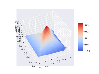
Figure 11: The function plot describing the difference between the two networks $N_{1}$ and $N_{2}$.

As mentioned in the last section, the training process of neural networks is approximate and can lead to many different solutions. A very natural question to ask is: “How differently do two neural networks solve the same problem?”. This question can be answered using algebraic operations on TADS.

Consider $N_{2}$, a PLNN that has also been trained with the network architecture shown in Figure 9, but with a different setting of hyperparameters. Its represented (semantic) function $f_{2}=\llbracket N_{2}\rrbracket_{\scriptscriptstyle\mathrm{DS}}$ is depicted in Figure 7b and the corresponding TADS $t_{2}=\tau(N_{2})$ in Figure 8b.

As TADS form a linear algebra, one can easily mirror the computation $f_{2}-f_{1}$ by $t_{2}-t_{1}$ on TADS level. The result is identical because the transformation process is precise, i.e.,

$$\llbracket N_{2}\rrbracket_{\scriptscriptstyle\mathrm{DS}}-\llbracket N_{1}\rrbracket_{\scriptscriptstyle\mathrm{DS}}=f_{2}-f_{1}=\llbracket t_{2}-t_{1}\rrbracket_{\scriptscriptstyle\mathrm{\Theta}}$$

The resulting difference TADS $t_{3}$ is shown in Figure 10 and the corresponding function graph in Figure 11.

The TADS $t_{3}$ is ideal to study the semantic difference between PLNN $N_{1}$ and$N_{2}$. Most interestingly, as can be visually seen in Figure 11, the largest differences between both networks occur in the middle of the function domain, i.e., in the region most distant from the edges where the XOR problem is clearly defined. This matches the intuition that points further away from known points are more uncertain under neural network training.

Further, observe that the difference of both networks yields a TADS of roughly double the size. This moderate increase in size indicates the similarity of $N_{1}$ and $N_{2}$, as linear regions of the difference TADS $t_{3}$ result from the intersection of the regions for $f_{1}$ and $f_{2}$ which could, in the worst case, grow quadratically.

As mentioned above (cf., Corollary 6.16), it is also possible to analyse $\epsilon$-similarity via algebraic operations to, in this case, obtain the TADS shown in Figure 12, which is much smaller than the full difference TADS (cf., Figure 10). The piece-wise affine function of this TADS is visualised in Figure 13.

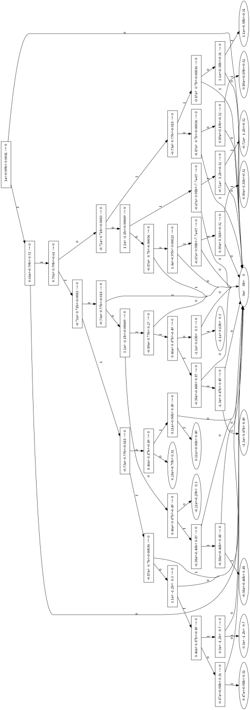
Figure 12: A TADS describing the difference between $f_{2}$ and $f_{1}$ iff it exceeds $\epsilon=0.3$.

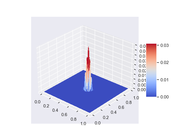
Figure 13: The function graph describing the difference between $f_{2}$ and $f_{1}$ iff it exceeds $\epsilon=0.3$

There are 8 regions in which the difference values exceed $0.3$, all close to the center of $[0,1]^{2}$. This, again matches the intuition that the volatility of solution grows with the distance to the defined values.

This result is interesting as it shows that, while the two neural networks that we trained differ, they do not differ more than $0.3$ except for a small region in the center of the input space. Similar constructions can be used to analyze robustness of neural networks. Robustness of neural networks is of large interest to neural network research [CW17] and the application of TADS to this problem is discussed in more detail in [NSMB23].

7.2 Classification

(a) TADS $t_{1}^{c}$ for the function $g_{1}=\mathbb{I}({x\geq 0.5})\circ f_{1}$

(b) TADS $t_{2}^{c}$ for the function $g_{2}=\mathbb{I}({x\geq 0.5})\circ f_{2}$

Figure 14: Classification TADS that indicates where the PLNNs $N_{1}$ and $N_{2}$ output a value greater than 0.5.

Figure 15: A TADS describing the function $\mathbb{I}({x\geq 0.5})$ that is used to transform the output of neural networks into discrete values.

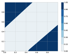
(a) ${g_{1}=\mathbb{I}({x\geq 0.5})\circ f_{1}}$ (cf., Figure 14a)

(b) ${g_{2}=\mathbb{I}({x\geq 0.5})\circ f_{2}}$ (cf., Figure 14b)

(c) $\llbracket t_{1}^{c}\ \ominus\ t_{2}^{c}\rrbracket_{\scriptscriptstyle\mathrm{\Theta}}$ (cf., Figure 17b)

Figure 16: Contour plots of the classification functions (a) $g_{1}$ and (b) $g_{2}$. The difference between both classifiers is visualized in (c).

Applications of neural networks are traditionally split into regression tasks and classification tasks. In regression tasks, one seeks to approximate a function with continuous values, whereas classification tasks have discrete outputs. As learned, piece-wise linear functions are inherently continuous, classification tasks require an additional step that interprets the continuous output of a neural network as one of multiple discrete classes. Note that this is a change of mindset, with the same neural network being interpreted differently depending on the context.

In our context, one might be interested in a model that classifies each input point $\vec{x}\in\mathbb{R}^{2}$ as either $1$ or $0$ instead of returning a real-value.

7.2.1 Class Characterization

A standard method for classification tasks is the interpretation of neural network outputs as a probability distribution over classes [GBC16]. In our XOR example, it is natural to interpret $f_{1}(\vec{x})$ as the probability of $\vec{x}$ belonging to class $1$ and $1-f_{1}(\vec{x})$ as the probability of $\vec{x}$ belonging to class $0$.

At evaluation time, one might naturally choose the class with the highest probability. Thus, $N_{1}$’s output is set to $1$ if it is greater than $0.5$ and $0$ otherwise, which is, actually, in line with the definition of $g_{*}$. Applying

$$\mathbb{I}(x\geq 0.5)=\begin{cases}1\quad&\text{if }x\geq 0.5\\ 0&\text{otherwise}\end{cases}.$$

to the continuous learned function $f_{1}$ therefore results in a suitable classifier for this problem:

$$g=\mathbb{I}(x\geq 0.5)\circ f_{1}$$

Note that $\mathbb{I}(x\geq 0.5)$ is not continuous and therefore cannot be represented by a PLNN.

To construct the TADS, we use the compositionality of TADS. We manually construct the simple TADS ${\tau(\mathbb{I}(x\geq 0.5))}$, as shown in Figure 15 and compose it with the TADS $t_{1}$ of $f_{1}$. The resulting TADS

$$t_{1}^{c}=\tau(\mathbb{I}(x\geq 0.5))\Join t_{1}$$

is shown in Figure 14a. Note that this TADS is reminiscent of a binary decision diagram with just two final nodes. Figure 16a and shows precisely which inputs are interpreted as $1$ and which as $0$. As we only have two classes here, this classification can be considered as what is called class characterization in [GS21] for both classes $0$ and $1$. Please note that class characterizations allows one to change the perspective from a classification task to the task of finding adequate candidates of specific profile, here given as a corresponding class.

This shows that, given an output interpretation that maps the continuous network outputs to discrete classes, it is possible to transform neural networks, fundamentally black-box representations of real valued functions, into semantically equivalent decision diagrams, fundamentally white-box representations of discrete valued functions.

7.2.2 Comparison of Classifiers

(a) TADS $t_{1}^{c}\ \ =⃝\ \ t_{2}^{c}$

(b) TADS $t_{1}^{c}\ \ominus\ t_{2}^{c}$

Figure 17: TADS representing the difference of the classification behavior of $N_{1}$ and $N_{2}$. The TADS in (a) expresses the equality of the classifications while (b) expresses the difference. Thus, by mapping the nodes $-1$ and $1$ to $0$ and $0$ to $1$ one can transform (b) to (a). Note, however, that despite their syntactical similarities, they represent different concepts.

After having constructed TADS that characterize the classification behavior of neural networks, we can also characterize the difference in classification behavior of two neural networks. We can simply do so by using the lifted equality relation to the TADS level and compute the TADS:

$$t_{1}^{c}\ \ =⃝\ \ t_{2}^{c}$$

The resulting TADS is shown in Figure 17a and the corresponding function graph in Figure 16c. This plot describes precisely the areas where both functions differ and where they coincide.

Notably, it shows that, while the absolute difference of $f_{1}$ and $f_{2}$ is highest in the center of the interval $[0,1]^{2}$, the networks agree in that area with respect to classification. Indeed, it appears that the largest difference with respect to classification occurs in the diagonals separating the classes $1$ and $0$. This is not too surprising, as it is at the borderline between classes were small changes may affect the classification result.

Using an encoding of boolean values as $1$ and $0$ respectively, we can also compute the difference of $t_{1}^{c}$ and $t_{2}^{c}$

$$t_{1}^{c}\ \ \ominus\ \ t_{2}^{c}$$

This TADS not only describes where $t_{1}^{c}$ and $t_{2}^{c}$ disagree, but also how they disagree. The corresponding TADS is shown in Figure 17b.

This shows the utility of TADS for output interpretation. While the absolute difference between two networks is a suitable measure of difference for regression tasks, the difference of the classification functions is suitable for classification. Playing with this difference, e.g., by modifying the classification function, is a powerful analytical instrument. E.g., in settings with many classes, separately analyzing the class characterizations of the individual classes typically leads to much smaller and easier to comprehend TADS and may therefore be a good means to increase scalability.

Figure 18: The TADS describing the difference between the baseline solution $\mathbb{I}(\lvert x-y\rvert\geq 0.5)$ and the solution learned by $N_{1}$.

In machine learning, one often compares learned classifiers to groundtruth solutions by sampling from the groundtruth solution and checking whether the neural network matches the groundtruth predictions. TADS enable a straightforward and precise way of evaluating a neural network in instances where one has access to the groundtruth model. E.g., the TADS of Figure 13 precisely specifies where $N_{1}$ differs from the baseline solution $\mathbb{I}(\lvert x-y\rvert\geq 0.5)$.

8 Related Work

The presented TADS-based approach towards understanding of neural networks is explicitly meant to bridge between the various existing initiative that aim in the same direction, but typically with quite different means. In this section, we review the state of the art under three perspectives:

• The intent, explainability, as approached in the neural networks community.

• Applied concepts, e.g., symbolic execution that aim at (locally) precise results.

• Applied background, in particular concerning piece-wise affine functions.

Whereas the first perspective (Section 8.1) is conceptually distant, both in its applied technologies as well as in its achievements, the mindset of second perspective (Section 8.2) is similar in aims and means, but, except for our previous work, restricts its attention to a locally precise analysis close to some (partly symbolic) input. The third perspective just concerns the mathematical background (Section 8.3). We are not aware of any previous work that systematically applies algebraic reasoning to achieve precise explanation and verification results about neural networks.

8.1 Machine Learning Explainability

In recent years, explainable AI (XAI) as a subfield of machine learning has seen a surge of activity. In line with existing machine learning research, XAI focuses on approaches that scale efficiently at the cost of precision and comprehensibility.

Due to vast amount of work in this direction we can only provide sketch of the field here, which from our perspective is characterized by is use of ‘traditional’ deep learning technologies such as gradient based optimization and its focus on directly investigating the neural networks themselves in an approximate fashion and without explicit link to some semantic model.

A typical example of a gradient-based method is activation maximization [MV16, SCD⁺17], which seeks to find, for one class $C$ and network $N$, the input $\vec{x}$ for which $\llbracket\vec{x}\rrbracket$ is maximal for class $C$. Being based on gradient based optimization, this approach is clearly approximate.

Other examples of approaches working on the neural network level are frequently found in attribution methods. Attribution methods focus on attributing a prediction $\llbracket N\rrbracket(\vec{x})=y$, to parts of the input that one deems responsible for this prediction. In general, this question is unclear and subjective. As a consequence, there exist multiple different methods that attribute the prediction differently to the original input. Examples include gradient based saliency maps [SVZ13, MCF19], layer-wise relevance propagation (LRP) [BBM⁺15] and deep taylor decomposition [MLB⁺17]. As attribution is natural to answer for linear models, these methods focus on linearly approximating the model (gradient based saliency maps) or parts of the model (LRP and deep taylor decomposition). The latter methods depend strongly on the neural network architecture and not on its semantics.

These methods are useful to gain rough intuition, but they do not offer any guarantees or reliable results. This is a direct consequence of most of these methods working with classical machine learning tools such as backpropagation and numerical optimization, which are fast but approximative [GBC16].

The class of XAI methods that is most closely related to TADS are local proxy models like LIME [RSG16] and SHAP [LL17]. Both methods consider one fixed input $\vec{x}$ and treat the model as a black-box. They observe the model’s behavior on multiple perturbations of the form $\vec{x}+p$ with $p$ being sampled randomly. Then, they use simple machine learning models such as a linear classifier or a decision tree to describe the model’s behavior on the perturbations $\vec{x}+p$ they observed.

These methods are similar in their intent to the TADS approach, as they use conceptually simple models to represent the black-box behavior of a neural network. However, both LIME and SHAP are imprecise. They both sample only a few points $\vec{x}+p$ in the neighborhood of $\vec{x}$ and might miss important properties of the neural network model. Further, both methods use a machine learning classifier to represent these points. These classifiers are usually linear models (or a comparably simple model) and cannot capture the full behavior of the network, which leads to potentially large and uncontrolled errors.

We are not aware of XAI methods that provide guarantees strong enough to justify a responsible use in safety critical applications.

8.2 Conceptually Related Work

Symbolic Execution of Neural Networks.

More closely related to TADS are approaches to explainability based on symbolic execution of neural networks.

The idea of explainability via symbolic (or rather concolic execution) of neural networks was already explored in the works of [GPW⁺19]. In their work, the authors translate a given PLNN into an imperative program and concolically execute one given input $\vec{x}\in\mathbb{R}^{n}$. This corresponds to exploring the one path of a TADS corresponding to $\vec{x}$. This yields the path condition and the affine transformation that are responsible for the prediction $N(\vec{x})$. The authors further use these explanations to find adversarial examples and find parts of an input that they deem important for a given classification. The results of this work are promising, but (very) local, as they restrict themselves to one linear region of the input.

The authors of [CHH⁺18] propose a method that closely mirrors the method of [GWZ⁺18]. In essence, both methods are almost identical, but differ in their conceptual derivation of the method. The authors of [CHH⁺18] also consider sets of predictions and work out what features act as discriminators in many of these predictions.

Moving from the idea of explanation, the authors of [SWR⁺18] consider concolic testing instead. Similar to the work of [GWZ⁺18], they execute singular inputs concolically. They use the results from concolic execution to heuristically derive new inputs that cover large areas of the input space.

TADS improve on these approaches in two ways. First, TADS offer a global viewpoint on neural network semantics, independent of a sample set. Second, TADS support algebraic operations on a conceptual level to derive globally precise explanation and verification results. As illustrated in Section 7, algebraic operations nicely serve as a toolbox to derive tailored and precise analyses.

Neural Network Verification.

Neural network verification aims to verify properties of neural networks, usually piece-wise linear neural networks using techniques from SMT-solving and abstract interpretation extended by domain-specific techniques [KBD⁺17, WZX⁺21, TMLM⁺19]. Verification approaches are usually precise, or at least provide a counterexample if a property is shown false. Modern solvers can scale quite well, but are still far from being able to tackle practically relevant applications [BLJ21].

Verification approaches are related to TADS as they also provide tools for the precise analysis of piece-wise linear neural networks. However, while SMT-based verification approaches currently scale better than TADS, they focus only on binary answers to a verification problem. They are not able to provide full diagnostics and descriptions of where and how an error occurs. However, please note, SMT-based approaches should not be considered as an alternative but rather as a provider of technologies that can also be applied at the TADS level. In fact, we use SMT solving, e.g., to eliminate infeasible paths in TADS.

Precise Explainability of Random Forests.

This work is conceptually closely related to and builds upon the work of [GS21, MNSB23]. There, ADDs are used and extended to derive explainable global models for random forests. Similar to the approach in this paper, these models are derived through a sequence of semantics-preserving transformations and later on refined by performing algebraic operations on the white-box representation of random forests. In fact, considering the underlying mindset, the work in this paper can be regarded as an extension of our work on random forest to neural networks. However, the much higher complexity of PLNN requires substantial generalization, which to our surprise did not clutter the theory, but rather added to its elegance.

8.3 Technologically Related Work

Linear Regions of Neural Networks.

Vast amounts of research have been conducted regarding the number and shape of linear regions in a given PLNN [Hin21, CHH⁺18, MPCB14, PMB13, ZW20, HR19b, STR18, HR19a, WL18, SKS⁺20, RPK⁺17, ABMM16]. Linear regions are of huge interest to neural network research as they give a natural characterization of the expressive power of neural network classes. This research is beneficial to the understanding of TADS as it can be used to bound the size of TADS and understand where and when explosions and size occur. On the other hand, TADS give a precise and minimal representation of the linear regions belonging to given neural network and can be used to facilitate experiments in this field, e.g., to find a linear region containing a negative example for a given property that could not be verified [KBD⁺17].

Structures for Polyhedral Sets.

At their core, TADS are efficient representations of multiple polyhedral regions within high-dimensional spaces. Similar problems occur in other divisions of computer science, most notably computer graphics.

TADS are closely related to Binary Space Partition Trees (BSP-trees) [TN87] and comparable structures [TJB03]. These structures are built to represent a partition of a real-dimensional space into polygons, much like TADS do. TADS extend these structures with optimizations from ADDs to account for domain-specific properties of piece-wise linear functions that are not present in the general case of polygonal partitions.

9 Conclusion and Future Work

We have presented an algebraic approach to the precise and global explanation of Rectifier Neural Networks (PLNNs), one of the most popular kinds of Neural Networks. Key to our approach is the symbolic execution of these networks that allows the construction of semantically equivalent Typed Affine Decision Structures (TADS). Due to their deterministic and sequential nature, TADS can be considered as white-box models and therefore as precise solutions to the model explanation problem, which directly imposes also solutions to the outcome explanation, and class characterization problems [GMS21, GS21]. Moreover, as linear algebras, TADS support operations that allows one to elegantly compare Rectifier Networks for equivalence or $\epsilon$-similarity, both with precise diagnostic information in case of failure, and to characterize their classification potential by precisely characterizing the set of inputs that are specifically classified, or the set of inputs where two Network-based classifiers differ. These are steps towards a more rigorous understanding of Neural Networks that is required when applying them in safety-critical domains without the possibility of human interference, such as self-driving cars.

This elegant situation at the semantic TADS level is in contrast with today’s practical reality where people directly work with learned PLNNs that are in particular characterized by their hidden layers that often comprise millions sometimes even billions of parameters. The reason for this complex structure is learning efficiency, a property paid for with semantic intractability: There is essentially no way to control the impact of minor changes of a parameter or input values, and even the mere evaluation for a sample input exceed the capacity of a human’s mind by far. This is why PLNNs are considered as black-box models.

The reason why TADS have not yet been studied may be due to their size: they may be exponentially larger than a corresponding PLNN. The reason for this expansion is the transformation of the incomprehensible hidden layers structure into a large decision structure, which conceptually is as easy to comprehend as a decision tree and a linear classifier. In this sense, our transformation into TADS can be regarded as trade of size for transparency, turning the verification and explanation problem into a scalability issue. There are at least three promising angles for attacking the scalability problem:

1. Learned PLNNs have a high amount of noise resulting from the underlying learning process that works by locally optimizing individual parameters of the hidden layers. Noise reduction may have a major impact on size. Detecting noise is clearly a semantic task and can therefore profit from TADS-based semantic analyses.

2. PLNNs are accepted to be approximate. Thus, controlled modifications with minor semantic impact are easily tolerated. TADS provide the means to control the effect of modifications and thereby to keep modifications in the tolerable range.

3. Modern neural network architectures are typically compositions of multiple sub-networks that are intended to support the learning of different subtasks. However, this structure at the representational layer gets semantically blurred during joint the learning process, which, e.g., prohibits compositional approaches as known from formal methods. The semantic transparency of TADS may provide means to reinforce the intended compositional structure also at the semantical level in order to support compositional reasoning and incremental construction.

Of course, there seems to be a hen/egg problem here. If we can construct the TADS, we are able to reduce it in order to achieve scalability. On the other hand, we need scalability first to construct the TADS. This is a well-known problem in the formal methods world, and despite a wealth of heuristics and domain-specific technologies, the answer is compositionality and incremental construction. This is exactly in line with the observation reported in the third item above: We need to learn how to use divide and conquer techniques for PLNN in a semantics-aware fashion. TADS are designed to support this quest by providing both a leading mindset and a tool-supported technology.

References

- [ABMM16] Raman Arora, Amitabh Basu, Poorya Mianjy, and Anirbit Mukherjee. Understanding deep neural networks with rectified linear units. arXiv preprint arXiv:1611.01491, 2016.
- [Axl97] Sheldon Axler. Linear algebra done right. Springer Science & Business Media, 1997.
- [BBC+19] Christopher Berner, Greg Brockman, Brooke Chan, Vicki Cheung, Przemysław Dębiak, Christy Dennison, David Farhi, Quirin Fischer, Shariq Hashme, Chris Hesse, et al. Dota 2 with large scale deep reinforcement learning. arXiv preprint arXiv:1912.06680, 2019.
- [BBM+15] Sebastian Bach, Alexander Binder, Grégoire Montavon, Frederick Klauschen, Klaus-Robert Müller, and Wojciech Samek. On pixel-wise explanations for non-linear classifier decisions by layer-wise relevance propagation. PloS one, 10(7):e0130140, 2015.
- [BFG+97] R. Iris Bahar, Erica A. Frohm, Charles M. Gaona, Gary D. Hachtel, Enrico Macii, Abelardo Pardo, and Fabio Somenzi. Algebric decision diagrams and their applications. Formal methods in system design, 10(2):171–206, 1997.
- [BGC+21] Claudine Badue, Rânik Guidolini, Raphael Vivacqua Carneiro, Pedro Azevedo, Vinicius B. Cardoso, Avelino Forechi, Luan Jesus, Rodrigo Berriel, Thiago M. Paixao, Filipe Mutz, et al. Self-driving cars: A survey. Expert Systems with Applications, 165:113816, 2021.
- [BLJ21] Stanley Bak, Changliu Liu, and Taylor Johnson. The second international verification of neural networks competition (vnn-comp 2021): Summary and results. arXiv preprint arXiv:2109.00498, 2021.
- [BMR+20] Tom Brown, Benjamin Mann, Nick Ryder, Melanie Subbiah, Jared D. Kaplan, Prafulla Dhariwal, Arvind Neelakantan, Pranav Shyam, Girish Sastry, Amanda Askell, et al. Language models are few-shot learners. Advances in neural information processing systems, 33:1877–1901, 2020.
- [Bro83] Arne Brondsted. An Introduction to Convex Polytopes. Springer, New York, NY, first edition, 1983.
- [CHH+18] Lingyang Chu, Xia Hu, Juhua Hu, Lanjun Wang, and Jian Pei. Exact and consistent interpretation for piecewise linear neural networks: A closed form solution. In Proceedings of the 24th ACM SIGKDD International Conference on Knowledge Discovery & Data Mining, pages 1244–1253, 2018.
- [Cla76] Lori A. Clarke. A system to generate test data and symbolically execute programs. IEEE Transactions on software engineering, (3):215–222, 1976.
- [CSW+18] Chung-Cheng Chiu, Tara N. Sainath, Yonghui Wu, Rohit Prabhavalkar, Patrick Nguyen, Zhifeng Chen, Anjuli Kannan, Ron J. Weiss, Kanishka Rao, Ekaterina Gonina, et al. State-of-the-art speech recognition with sequence-to-sequence models. In 2018 IEEE International Conference on Acoustics, Speech and Signal Processing (ICASSP), pages 4774–4778. IEEE, 2018.
- [CW17] Nicholas Carlini and David Wagner. Towards evaluating the robustness of neural networks. In 2017 ieee symposium on security and privacy (sp), pages 39–57. IEEE, 2017.
- [DSB17] Derek Doran, Sarah Schulz, and Tarek R. Besold. What does explainable AI really mean? a new conceptualization of perspectives. arXiv preprint arXiv:1710.00794, 2017.
- [GBB11] Xavier Glorot, Antoine Bordes, and Yoshua Bengio. Deep sparse rectifier neural networks. In Proceedings of the fourteenth international conference on artificial intelligence and statistics, pages 315–323. JMLR Workshop and Conference Proceedings, 2011.
- [GBC16] Ian Goodfellow, Yoshua Bengio, and Aaron Courville. Deep Learning. MIT Press, 2016. http://www.deeplearningbook.org.
- [GMR+18] Riccardo Guidotti, Anna Monreale, Salvatore Ruggieri, Franco Turini, Fosca Giannotti, and Dino Pedreschi. A survey of methods for explaining black box models. ACM Comput. Surv., 51(5), August 2018.
- [GMS21] Frederik Gossen, Tiziana Margaria, and Bernhard Steffen. Formal methods boost experimental performance for explainable ai. IT Professional, 23(6):8–12, 2021.
- [GPW+19] Divya Gopinath, Corina S. Pasareanu, Kaiyuan Wang, Mengshi Zhang, and Sarfraz Khurshid. Symbolic execution for attribution and attack synthesis in neural networks. In 2019 IEEE/ACM 41st International Conference on Software Engineering: Companion Proceedings (ICSE-Companion), pages 282–283. IEEE, 2019.
- [GS21] Frederik Gossen and Bernhard Steffen. Algebraic aggregation of random forests: towards explainability and rapid evaluation. International Journal on Software Tools for Technology Transfer, 2021.
- [GSS14] Ian J. Goodfellow, Jonathon Shlens, and Christian Szegedy. Explaining and harnessing adversarial examples. arXiv preprint arXiv:1412.6572, 2014.
- [GWZ+18] Divya Gopinath, Kaiyuan Wang, Mengshi Zhang, Corina S. Pasareanu, and Sarfraz Khurshid. Symbolic execution for deep neural networks. arXiv preprint arXiv:1807.10439, 2018.
- [GZB94] Valentin V. Gorokhovik, Oleg I. Zorko, and G. Birkhoff. Piecewise affine functions and polyhedral sets. Optimization, 31(3):209–221, 1994.
- [Hin21] Peter Hinz. Using activation histograms to bound the number of affine regions in ReLU feed-forward neural networks. ArXiv, abs/2103.17174, 2021.
- [HLXZ18] Juncai He, Lin Li, Jinchao Xu, and Chunyue Zheng. ReLU deep neural networks and linear finite elements. arXiv preprint arXiv:1807.03973, 2018.
- [HR19a] Boris Hanin and David Rolnick. Complexity of linear regions in deep networks. In Kamalika Chaudhuri and Ruslan Salakhutdinov, editors, Proceedings of the 36th International Conference on Machine Learning, volume 97 of Proceedings of Machine Learning Research, pages 2596–2604. PMLR, 09–15 Jun 2019.
- [HR19b] Boris Hanin and David Rolnick. Deep relu networks have surprisingly few activation patterns. Advances in neural information processing systems, 32, 2019.
- [KB14] Diederik P. Kingma and Jimmy Ba. Adam: A method for stochastic optimization. arXiv preprint arXiv:1412.6980, 2014.
- [KBD+17] Guy Katz, Clark Barrett, David L. Dill, Kyle Julian, and Mykel J. Kochenderfer. Reluplex: An efficient SMT solver for verifying deep neural networks. In International conference on computer aided verification, pages 97–117. Springer, 2017.
- [Kin76] James C. King. Symbolic execution and program testing. Communications of the ACM, 19(7):385–394, 1976.
- [LL17] Scott M. Lundberg and Su-In Lee. A unified approach to interpreting model predictions. Advances in neural information processing systems, 30, 2017.
- [LPK21] Pantelis Linardatos, Vasilis Papastefanopoulos, and Sotiris Kotsiantis. Explainable ai: A review of machine learning interpretability methods. Entropy, 23(1):18, 2021.
- [MCF19] T. Nathan Mundhenk, Barry Y. Chen, and Gerald Friedland. Efficient saliency maps for explainable ai. arXiv preprint arXiv:1911.11293, 2019.
- [MLB+17] Grégoire Montavon, Sebastian Lapuschkin, Alexander Binder, Wojciech Samek, and Klaus-Robert Müller. Explaining nonlinear classification decisions with deep taylor decomposition. Pattern recognition, 65:211–222, 2017.
- [MMS+17] Aleksander Madry, Aleksandar Makelov, Ludwig Schmidt, Dimitris Tsipras, and Adrian Vladu. Towards deep learning models resistant to adversarial attacks. arXiv preprint arXiv:1706.06083, 2017.
- [MNSB23] Alnis Murtovi, Gerrit Nolte, Maximilian Schlüter, and Steffen Bernhard. Forest Gump: A tool for veification and explanation. In this issue, 2023.
- [MP69] Marvin Minsky and Seymour Papert. Perceptrons. 1969.
- [MPCB14] Guido F. Montufar, Razvan Pascanu, Kyunghyun Cho, and Yoshua Bengio. On the number of linear regions of deep neural networks. Advances in neural information processing systems, 27, 2014.
- [MV16] Aravindh Mahendran and Andrea Vedaldi. Visualizing deep convolutional neural networks using natural pre-images. International Journal of Computer Vision, 120(3):233–255, 2016.
- [NSMB23] Gerrit Nolte, Maximilian Schlüter, Alnis Murtovi, and Steffen Bernhard. The power of Typed Affine Decision Structures: A case study. In this issue, 2023.
- [OJ04] Kyoung-Su Oh and Keechul Jung. GPU implementation of neural networks. Pattern Recognition, 37(6):1311–1314, 2004.
- [Ovc10] Sergei Ovchinnikov. Discrete piecewise linear functions. European Journal of Combinatorics, 31(5):1283–1294, 2010.
- [PMB13] Razvan Pascanu, Guido Montufar, and Yoshua Bengio. On the number of response regions of deep feed forward networks with piece-wise linear activations. arXiv preprint arXiv:1312.6098, 2013.
- [RPK+17] Maithra Raghu, Ben Poole, Jon Kleinberg, Surya Ganguli, and Jascha Sohl-Dickstein. On the expressive power of deep neural networks. In international conference on machine learning, pages 2847–2854. PMLR, 2017.
- [RSG16] Marco Tulio Ribeiro, Sameer Singh, and Carlos Guestrin. " why should i trust you?" explaining the predictions of any classifier. In Proceedings of the 22nd ACM SIGKDD international conference on knowledge discovery and data mining, pages 1135–1144, 2016.
- [Rud16] Sebastian Ruder. An overview of gradient descent optimization algorithms. arXiv preprint arXiv:1609.04747, 2016.
- [SCD+17] Ramprasaath R. Selvaraju, Michael Cogswell, Abhishek Das, Ramakrishna Vedantam, Devi Parikh, and Dhruv Batra. Grad-cam: Visual explanations from deep networks via gradient-based localization. In Proceedings of the IEEE international conference on computer vision, pages 618–626, 2017.
- [SKS+20] A. Sudjianto, William Knauth, Rahul Singh, Zebin Yang, and Aijun Zhang. Unwrapping the black box of deep ReLU networks: Interpretability, diagnostics, and simplification. ArXiv, abs/2011.04041, 2020.
- [Sob15] Elliott Sober. Ockham’s razors. Cambridge University Press, 2015.
- [SSS+17] David Silver, Julian Schrittwieser, Karen Simonyan, Ioannis Antonoglou, Aja Huang, Arthur Guez, Thomas Hubert, Lucas Baker, Matthew Lai, Adrian Bolton, et al. Mastering the game of go without human knowledge. nature, 550(7676):354–359, 2017.
- [STR18] Thiago Serra, Christian Tjandraatmadja, and Srikumar Ramalingam. Bounding and counting linear regions of deep neural networks. In International Conference on Machine Learning, pages 4558–4566. PMLR, 2018.
- [SVZ13] Karen Simonyan, Andrea Vedaldi, and Andrew Zisserman. Deep inside convolutional networks: Visualising image classification models and saliency maps. arXiv preprint arXiv:1312.6034, 2013.
- [SWR+18] Youcheng Sun, Min Wu, Wenjie Ruan, Xiaowei Huang, Marta Kwiatkowska, and Daniel Kroening. Concolic testing for deep neural networks. In Proceedings of the 33rd ACM/IEEE International Conference on Automated Software Engineering, pages 109–119, 2018.
- [SZ14] Karen Simonyan and Andrew Zisserman. Very deep convolutional networks for large-scale image recognition. arXiv preprint arXiv:1409.1556, 2014.
- [SZS+13] Christian Szegedy, Wojciech Zaremba, Ilya Sutskever, Joan Bruna, Dumitru Erhan, Ian Goodfellow, and Rob Fergus. Intriguing properties of neural networks. arXiv preprint arXiv:1312.6199, 2013.
- [TG20] Erico Tjoa and Cuntai Guan. A survey on explainable artificial intelligence (xai): Toward medical xai. IEEE transactions on neural networks and learning systems, 32(11):4793–4813, 2020.
- [TJB03] P. Tøndel, T. A. Johansen, and A. Bemporad. Evaluation of piecewise affine control via binary search tree. Automatica, 39(5):945–950, 2003.
- [TMLM+19] Hoang-Dung Tran, Diago Manzanas Lopez, Patrick Musau, Xiaodong Yang, Luan Viet Nguyen, Weiming Xiang, and Taylor T. Johnson. Star-based reachability analysis of deep neural networks. In International symposium on formal methods, pages 670–686. Springer, 2019.
- [TN87] William C. Thibault and Bruce F. Naylor. Set operations on polyhedra using binary space partitioning trees. In Proceedings of the 14th annual conference on Computer graphics and interactive techniques, pages 153–162, 1987.
- [VBC+19] Oriol Vinyals, Igor Babuschkin, Wojciech M. Czarnecki, Michaël Mathieu, Andrew Dudzik, Junyoung Chung, David H. Choi, Richard Powell, Timo Ewalds, Petko Georgiev, et al. Grandmaster level in StarCraft II using multi-agent reinforcement learning. Nature, 575(7782):350–354, 2019.
- [WL18] Seongyoun Woo and Chulhee Lee Lee. Decision boundary formation of deep convolution networks with ReLU. In 2018 IEEE 16th Intl Conf on Dependable, Autonomic and Secure Computing, 16th Intl Conf on Pervasive Intelligence and Computing, 4th Intl Conf on Big Data Intelligence and Computing and Cyber Science and Technology Congress (DASC/PiCom/DataCom/CyberSciTech), pages 885–888. IEEE, 2018.
- [WZX+21] Shiqi Wang, Huan Zhang, Kaidi Xu, Xue Lin, Suman Jana, Cho-Jui Hsieh, and J. Zico Kolter. Beta-crown: Efficient bound propagation with per-neuron split constraints for complete and incomplete neural network verification. arXiv preprint arXiv:2103.06624, 2021.
- [ZW20] Xiao Zhang and Dongrui Wu. Empirical studies on the properties of linear regions in deep neural networks. arXiv preprint arXiv:2001.01072, 2020.