Quadrupole transitions and quantum gates protected by continuous dynamic decoupling

Abstract

Dynamical decoupling techniques are a versatile tool for engineering quantum states with tailored properties. In trapped ions, nested layers of continuous dynamical decoupling by means of radio-frequency field dressing can cancel dominant magnetic and electric shifts and therefore provide highly prolonged coherence times of electronic states. Exploiting this enhancement for frequency metrology, quantum simulation or quantum computation, poses the challenge to combine the decoupling with laser-ion interactions for the quantum control of electronic and motional states of trapped ions. Ultimately, this will require running quantum gates on qubits from dressed decoupled states. We provide here a compact representation of nested continuous dynamical decoupling in trapped ions, and apply it to electronic $S$ and $D$ states and optical quadrupole transitions. Our treatment provides all effective transition frequencies and Rabi rates, as well as the effective selection rules of these transitions. On this basis, we discuss the possibility of combining continuous dynamical decoupling and Mølmer-Sørensen gates.

I Introduction

Since the early work of Hahn on spin echoes in nuclear magnetic resonance (NMR) Hahn (1950), techniques for dynamically decoupling a quantum system from its environment to increase its coherence times have become indispensable tools of quantum technology Souza et al. (2012), with applications in quantum simulations, computation, and metrology. Robust dynamic decoupling methods by applying external pulses have been intensively developed both in theory Viola and Lloyd (1998); Viola et al. (1999); Zanardi (1999); Byrd and Lidar (2002); Facchi et al. (2005); Khodjasteh and Lidar (2008); Khodjasteh and Viola (2009a, b); Khodjasteh et al. (2010); D.A (2012); Aharon et al. (2019); Green et al. (2013); West et al. (2010); Uhrig (2007); Haeberlen and Waugh (1968) and in experiment Biercuk et al. (2009); Du et al. (2009); Damodarakurup et al. (2009); de Lange et al. (2010); Souza et al. (2011); Naydenov et al. (2011); van der Sar et al. (2012); Shaniv et al. (2019); Wang et al. (2017); Qiu et al. (2021); Zhou et al. (2020); Manovitz et al. (2017); Shaniv et al. (2016); Piltz et al. (2013); de Lange et al. (2010). In recent years, continuous dynamical decoupling (CDD), where control pulses are applied in the form of continuous time periodic fields in the spirit of Floquet engineering Kuwahara et al. (2016), have been proposed and demonstrated Fonseca-Romero et al. (2005); Chen (2006); Yalçınkaya et al. (2019); Clausen et al. (2010); Xu et al. (2012); Fanchini et al. (2007); Fanchini and Napolitano (2007); Fanchini et al. (2015); Rabl et al. (2009); Chaudhry and Gong (2012); Cai et al. (2012); Laraoui and Meriles (2011); Shaniv et al. (2019); Bermudez et al. (2011, 2012); Timoney et al. (2011); Doherty et al. (2013); Albrecht et al. (2014); Golter et al. (2014); Finkelstein et al. (2021); Trypogeorgos et al. (2018); Anderson et al. (2018); Laucht et al. (2017); Sárkány et al. (2014); Webster et al. (2013); Tan et al. (2013); Aharon et al. (2013); Zanon-Willette et al. (2012).

The design of long-lived quantum states using CDD has promising perspectives, especially for trapped ion frequency metrology as proposed and studied in Cai et al. (2012); Aharon et al. (2019); Shaniv et al. (2019). The statistical uncertainty for a given clock species can be improved by extending the probe time, which will ultimately be limited by the lifetime of the excited states Kessler et al. (2014). Nevertheless, in practice, it is usually limited by the coherence time of the clock laser Peik et al. (2005); Leroux et al. (2017). We can also improve the statistical uncertainty by interrogating many atoms simultaneously Keller et al. (2019); Arnold et al. (2015); Herschbach et al. (2012); Champenois et al. (2010). But increasing the number of ions stored in a Paul trap entails further obstacles to overcome. Depending on the ion species chosen, inhomogeneous or time-dependent frequency shifts, such as the Zeeman shift, the Quadrupole shift, or the radio frequency (rf) electric field-induced tensor ac Stark shift Itano (2000); Berkeland et al. (1998); Arnold et al. (2015), pose a limitation. These effects can contribute to the decoherence of the state or broaden the joint linewidth of the ions, thus limiting the usable probe time. Several approaches exist to constrain the tensor-like electric field shifts even without exact knowledge of the electric field gradient. One approach consists in averaging over different transitions or directions to exploit the different scaling of the shift with the angular momentum component Itano (2000); Schneider et al. (2005); Dubé et al. (2005), or by chosing a magnetic field direction along which the tensor shifts have a zero crossing Tan et al. (2019). Another method dynamically changes the static offset B-field direction within the clock interrogation Lange et al. (2020) to mimic the magic angle spinning technique of nuclear magnetic resonance spectroscopy Andrew et al. (1958). Elimination of these shifts can also be achieved by suitable hyperfine or Zeeman averaging using DD Kaewuam et al. (2020); Shaniv et al. (2019). Achieving robust optical clock transitions protected by CDD has been explored by Aharon et al. Aharon et al. (2019).

In order to exploit these tailored states for quantum metrology, possibly involving entangled states of many ions, dynamical decoupling has to be combined with laser-ion interaction on optical quadrupole transitions, which will be the focus of the current work. Following the work of Aharon et. al. Aharon et al. (2019) we reformulate the CDD description to easily treat the laser ion interaction. We begin by recapitulating the dynamical decoupling principle for a particular spin manifold, which is subject to a Zeeman splitting controlled by a static dc magnetic field, showing the effective Hamiltonian in the so-called doubly-dressed basis. Here, modulated external rf magnetic fields are employed to mitigate the amplitude-induced line shifts Aharon et al. (2019). Then, with appropriate CDD parameters, we achieve suppression of Zeeman and quadrupole shifts in this basis. Next, we consider optical quadrupole transitions between two of these spin manifolds and characterize the laser-ion interaction needed to drive the above transitions. We will show that there is no selection rule for transitions in the doubly-dressed basis. The only necessary condition will be the proper detuning of the laser. The suppression of Zeeman and quadrupole shifts will come at the cost of a reduction of the effective Rabi frequency for these transitions, and therefore, the characterization of these transitions will allow us to choose an appropriate candidate for a clock transition. We compare our analytical treatment with measurements of CDD states of a single ${}^{40}\mathrm{Ca}^{+}$ ion. Measurements of the energy spectrum between different spin manifolds as well as their relative optical coupling are in good agreement with the predictions. We will finish by discussing the application of a Mølmer-Sørensen gate in the doubly dressed basis, discussing its challenges and calculating a theoretical prediction for the gate time.

The article is organized as follows: In Section II we reformulate the CDD description showing the suppression of Zeeman and quadrupole shifts for the appropiate parameters. The characterization of the optical transitions among two doubly-dressed manifolds through laser interaction, as well as the application to a trapped ${}^{40}\mathrm{Ca}^{+}$ ion is discussed in Section 2. In Section IV the experiment is described along with a comparison of the predicted and measured first stage CDD spectrum. Finally in Section V we motivate the application of a Mølmer-Sørensen gate and study the time gate for the case of a trapped ${}^{40}\mathrm{Ca}^{+}$ ion.

II Dynamical Decoupling

In this section, we recapitulate the principle of dynamical decoupling for the suppression of Zeeman and quadrupole shifts by applying radiofrequency magnetic fields Cai et al. (2012); Aharon et al. (2019); Shaniv et al. (2019). Although we will eventually consider quadrupole transitions from a spin-$S^{\mathrm{s}}$ manifold of ground states to a spin-$S^{\mathrm{d}}$ manifold of excited states, it will be useful to first examine how the dressing fields affect a single spin-$S$ manifold. This will facilitate the discussion of the physical principle of dynamical decoupling. Moreover, this will separate the effects associated with the problem of a single manifold from those associated with the cross-coupling of spin manifolds, which we will consider later.

II.1 Doubly-dressed basis

We will consider a manifold of total spin $S$ with $\mathbf{S}=(S_{x},S_{y},S_{z})$, basis states $\ket*{M}$, $|M|\leq S$, and quantization axis along $z$. If a static magnetic field $B$ along the $z$-axis is present, the internal states $\ket*{M}$ will be shifted by a value proportional to their spin, due to the linear Zeeman effect. Therefore, the Hamiltonian will have the expression

$$H_{\mathrm{dc}}=g\mu_{B}BS_{z}=\omega_{0}S_{z},$$ (1)

where $g$ is the gyromagnetic factor, the corresponding Larmor frequency is $\omega_{0}=g\mu_{B}B$, with $\mu_{B}$ being the Bohr magnetron, and we set $\hbar=1$. The eigenstates of this Hamiltonian will be referred to as bare states. A radio-frequency field $B_{\mathrm{rf}}(t)$ is applied with a polarisation in the $x-y$ plane, which for the sake of generality we consider enclosing an angle $\alpha$ with the $x$-axis. The ${\mathrm{rf}}$ field $B_{\mathrm{rf}}(t)$ is assumed to comprise frequency components at a fundamental frequency $\omega_{1}$ and sideband frequencies $\omega_{1}\pm\omega_{2}$, where $\omega_{2}<\omega_{1}$, such that the Hamiltonian for the rf fields is

$$H_{{\mathrm{rf}}} =g\quantity\big(\Omega_{1}\cos(\omega_{1}t)-\Omega_{2}\sin(\omega_{1}t)\cos(\omega_{2}t))$$

$$\quad\times(S_{x}\cos\alpha+S_{y}\sin\alpha),$$ (2)

where $\Omega_{1}$ and $\Omega_{2}$ are set by the amplitudes of the fundamental and sideband components of the rf-magnetic field, respectively. Therefore, the total Hamiltonian for the spin $S$ in the laboratory frame (LF) is

$$H^{\mathrm{LF}}=H_{\mathrm{dc}}+H_{{\mathrm{rf}}}.$$ (3)

To help characterize the rf or dressing fields, we are going to introduce a series of transformations into several frames. In this sequence of transformations we will denote a unitary rotation around an axis $\mathbf{n}$ about an angle $\theta$ by

$$U_{\mathbb{n}}(\theta)=\exp\quantity(\mathrm{i}\theta\mathbf{n}\mathbf{S}),$$ (4)

and use the notation

$$\mathcal{R}_{\mathbb{n}}(\theta)A\coloneqq U^{\phantom{\dagger}}_{\mathbb{n}}(\theta)AU^{\dagger}_{\mathbb{n}}(\theta),$$ (5)

for the superoperator corresponding to the conjugation of an operator $A$ with $U_{\mathbb{n}}(\theta)$. Bold symbols denote three-vectors. To determine the Hamiltonian operator $H$ in a new reference system, we consider the transformation of the operator $H-\mathrm{i}\derivative{t}$ in each case so that the time dependence of the transformation is properly accounted for. This will be useful when dealing with sequences of transformations.

First, we go into a frame rotating around the $z$-axis at the rf frequency $\omega_{1}$

$$\mathcal{R}_{\mathbb{z}}(\omega_{1}t)\quantity[H^{\mathrm{LF}}-\mathrm{i}\textstyle{\derivative{t}}]$$

$$=\quantity(\mathcal{R}_{\mathbb{z}}(\omega_{1}t)H^{\mathrm{LF}})-\omega_{1}S_{z}-\mathrm{i}\derivative{t}$$

$$=\Delta_{1}S_{z}+\frac{g\Omega_{1}}{2}(S_{x}\cos\alpha+S_{y}\sin\alpha)$$ (6)

$$\quad+\frac{g\Omega_{2}}{2}\cos(\omega_{2}t)(S_{y}\cos\alpha-S_{x}\sin\alpha)-\mathrm{i}\derivative{t}.$$

Here, we have defined the detuning of the rf-field with respect to the Larmor frequency $\Delta_{1}=\omega_{0}-\omega_{1}$. We have also used a rotating wave approximation (RWA) and dropped terms oscillating at $2\omega_{1}$, assuming $2\omega_{1}\gg g\Omega_{1}/2$. The effective contribution of these counter rotating terms on the bare states is addressed in Appendix C.

In the next step, the Hamiltonian is rewritten in the dressed state basis corresponding to the eigenstates of the time-independent part of the Hamiltonian on the right-hand side of Eq. (II.1), which correspond to the first line in the right-hand side. We achieve this by a rotation around an axis $\mathbb{n}_{1}=(-\sin\alpha,\cos\alpha,0)$ and an angle $\theta_{1}\in\left[0,\pi\right]$ defined by $\cos\theta_{1}=\Delta_{1}/\mkern 1.7mu\hbox{\vbox{\hrule height=0.4pt\kern 1.29167pt\hbox{\kern 0.0pt$\mkern-1.7mu\omega\mkern-1.7mu$\kern 0.0pt}}}\mkern 1.7mu_{0}$, where

$$\mkern 1.7mu\hbox{\vbox{\hrule height=0.4pt\kern 1.29167pt\hbox{\kern 0.0pt$\mkern-1.7mu\omega\mkern-1.7mu$\kern 0.0pt}}}\mkern 1.7mu_{0}=\quantity(\Delta_{1}^{2}+g^{2}\Omega^{2}_{1}/4)^{1/2}.$$ (7)

The Hamiltonian in this first dressed basis is

$$\mathcal{R}_{\mathbb{n_{\text{1}}}}(\theta_{1})\mathcal{R}_{\mathbb{z}}(\omega_{1}t)\quantity[H^{\mathrm{LF}}-\mathrm{i}\textstyle{\derivative{t}}]$$

$$=\mkern 1.7mu\hbox{\vbox{\hrule height=0.4pt\kern 1.29167pt\hbox{\kern 0.0pt$\mkern-1.7mu\omega\mkern-1.7mu$\kern 0.0pt}}}\mkern 1.7mu_{0}S_{z}+\frac{g\Omega_{2}}{2}\cos(\omega_{2}t)(S_{y}\cos\alpha-S_{x}\sin\alpha)-\mathrm{i}\derivative{t}.$$ (8)

This Hamiltonian refers to a new time-dependent quantization axis enclosing an angle $\theta_{1}$ with the $z$-axis. The relation between the bare basis and the dressed basis and their respective quantization axis and energy splittings $\hbar\omega_{0}$ and $\hbar\mkern 1.7mu\hbox{\vbox{\hrule height=0.4pt\kern 1.29167pt\hbox{\kern 0.0pt$\mkern-1.7mu\omega\mkern-1.7mu$\kern 0.0pt}}}\mkern 1.7mu_{0}$ are shown in Fig. 1. In the regime considered here, these frequencies satisfy the hierarchy $\omega_{0}\gg\mkern 1.7mu\hbox{\vbox{\hrule height=0.4pt\kern 1.29167pt\hbox{\kern 0.0pt$\mkern-1.7mu\omega\mkern-1.7mu$\kern 0.0pt}}}\mkern 1.7mu_{0}$.

Figure 1: Sketch of dynamical decoupling effect on a spin manifold (here $S=3/2$). (a) illustrates the quantization axis and (b) the energy splitting $\omega_{1}$ of bare basis states $\ket{m}$ and the rf drive at Rabi frequency $\Omega_{1}$ and detuning $\Delta_{1}$. (c) shows the quantization with one layer of dressing, and (d) the effective level scheme of the dressed levels $\ket{\mkern 1.7mu\hbox{\vbox{\hrule height=0.4pt\kern 1.29167pt\hbox{\kern 0.0pt$\mkern-1.7mum\mkern-1.7mu$\kern 0.0pt}}}\mkern 1.7mu}$ with splitting $\mkern 1.7mu\hbox{\vbox{\hrule height=0.4pt\kern 1.29167pt\hbox{\kern 0.0pt$\mkern-1.7mu\omega\mkern-1.7mu$\kern 0.0pt}}}\mkern 1.7mu_{0}$. (b) and (d) are not to scale as $\mkern 1.7mu\hbox{\vbox{\hrule height=0.4pt\kern 1.29167pt\hbox{\kern 0.0pt$\mkern-1.7mu\omega\mkern-1.7mu$\kern 0.0pt}}}\mkern 1.7mu_{0}\ll\omega_{0}$.

The next dressing layer consists of the same two types of transformations as the first one. First, the system is transformed into the rotating frame with frequency $\omega_{2}$ around the new quantization axis, where fast oscillating terms $2\omega_{2}\gg g\Omega_{2}/4$ are neglected. Then, a transformation is applied in a new basis that diagonalizes the Hamiltonian, now independent of time. The transformation that achieves this corresponds to a rotation by an axis $\mathbb{n}_{2}=(-\cos\alpha,-\sin\alpha,0)$ and the angle $\theta_{2}$ where $\cos\theta_{2}=\Delta_{2}/\mkern 1.7mu\hbox{\vbox{\hrule height=0.4pt\kern 0.86108pt\hbox{\kern 0.0pt$\mkern-1.7mu\mkern 1.7mu\hbox{\vbox{\hrule height=0.4pt\kern 1.29167pt\hbox{\kern 0.0pt$\mkern-1.7mu\omega\mkern-1.7mu$\kern 0.0pt}}}\mkern 1.7mu\mkern-1.7mu$\kern 0.0pt}}}\mkern 1.7mu_{0}$, and

$$\mkern 1.7mu\hbox{\vbox{\hrule height=0.4pt\kern 0.86108pt\hbox{\kern 0.0pt$\mkern-1.7mu\mkern 1.7mu\hbox{\vbox{\hrule height=0.4pt\kern 1.29167pt\hbox{\kern 0.0pt$\mkern-1.7mu\omega\mkern-1.7mu$\kern 0.0pt}}}\mkern 1.7mu\mkern-1.7mu$\kern 0.0pt}}}\mkern 1.7mu_{0}=\quantity(\Delta_{2}^{2}+g^{2}\Omega^{2}_{2}/16)^{1/2}.$$ (9)

The detuning at the second dressing layer is $\Delta_{2}=\mkern 1.7mu\hbox{\vbox{\hrule height=0.4pt\kern 1.29167pt\hbox{\kern 0.0pt$\mkern-1.7mu\omega\mkern-1.7mu$\kern 0.0pt}}}\mkern 1.7mu_{0}-\omega_{2}$. This results in the final, doubly-dressed Hamiltonian

$$\mathcal{R}_{\mathbb{n_{\text{2}}}}(\theta_{2})\mathcal{R}_{\mathbb{z}}(\omega_{2}t)\mathcal{R}_{\mathbb{n_{\text{1}}}}(\theta_{1})\mathcal{R}_{\mathbb{z}}(\omega_{1}t)\quantity[H^{\mathrm{LF}}-\mathrm{i}\textstyle{\derivative{t}}]$$

$$=\mkern 1.7mu\hbox{\vbox{\hrule height=0.4pt\kern 0.86108pt\hbox{\kern 0.0pt$\mkern-1.7mu\mkern 1.7mu\hbox{\vbox{\hrule height=0.4pt\kern 1.29167pt\hbox{\kern 0.0pt$\mkern-1.7muH\mkern-1.7mu$\kern 0.0pt}}}\mkern 1.7mu\mkern-1.7mu$\kern 0.0pt}}}\mkern 1.7mu-\mathrm{i}\derivative{t}$$ (10)

where the Hamiltonian in the doubly-dressed basis is

    $$\mkern-1.7muH\mkern-1.7mu =\mkern 1.7mu\hbox{\vbox{\hrule height=0.4pt\kern 0.86108pt\hbox{\kern 0.0pt$\mkern-1.7mu\mkern 1.7mu\hbox{\vbox{\hrule height=0.4pt\kern 1.29167pt\hbox{\kern 0.0pt$\mkern-1.7mu\omega\mkern-1.7mu$\kern 0.0pt}}}\mkern 1.7mu\mkern-1.7mu$\kern 0.0pt}}}\mkern 1.7mu_{0}S_{z}.$$ (11)

The quantization axis of the Hamiltonian in Eq. (II.1) is now again rotated at an angle $\theta_{2}$ with respect to the previous one. In principle, further dressing layers can be added, which will correspond to a similar sequence of transformations. Applications of $n$ layers of dressing have been discussed by Cai et al. Cai et al. (2012). We note that we will use symbols with single and double overbars (such as $\mkern 1.7mu\hbox{\vbox{\hrule height=0.4pt\kern 1.29167pt\hbox{\kern 0.0pt$\mkern-1.7mu\omega\mkern-1.7mu$\kern 0.0pt}}}\mkern 1.7mu_{0}$ and $\mkern 1.7mu\hbox{\vbox{\hrule height=0.4pt\kern 0.86108pt\hbox{\kern 0.0pt$\mkern-1.7mu\mkern 1.7mu\hbox{\vbox{\hrule height=0.4pt\kern 1.29167pt\hbox{\kern 0.0pt$\mkern-1.7mu\omega\mkern-1.7mu$\kern 0.0pt}}}\mkern 1.7mu\mkern-1.7mu$\kern 0.0pt}}}\mkern 1.7mu_{0}$) to denote quantities in the singly or doubly dressed frame, respectively.

We emphasize that the dressing procedure involves two rotating wave approximations, which are implicit in Eq. (II.1), and are based on $2\omega_{i}\gg g\Omega_{i}/2^{i}$ for $i=1,2$. Thus, we have the hierarchy $\mkern 1.7mu\hbox{\vbox{\hrule height=0.4pt\kern 0.86108pt\hbox{\kern 0.0pt$\mkern-1.7mu\mkern 1.7mu\hbox{\vbox{\hrule height=0.4pt\kern 1.29167pt\hbox{\kern 0.0pt$\mkern-1.7mu\omega\mkern-1.7mu$\kern 0.0pt}}}\mkern 1.7mu\mkern-1.7mu$\kern 0.0pt}}}\mkern 1.7mu_{0}\ll\omega_{2}\ll\omega_{1}$. Nevertheless, the terms neglected during the RWA will be accounted for perturbatively using the Magnus expansion in appendix C. We note that, instead of the perturbative treatment given here, it is also possible to determine the exact quasi-energy eigenstates of the time-periodic Hamiltonian in the laboratory frame in the framework of Floquet theory. However, since this analysis provides mainly numerical insight, we focus on the analytical perturbative treatment in this presentation. We checked numerically that this treatment is in excellent agreement with the dc component of the Floquet states when counter-rotating terms are accounted for in a Magnus expansion Martínez (2022).

II.2 Suppression of Zeeman and quadrupole shifts

In this section we briefly discuss how the two layers of dressing help to suppress linear Zeeman and electric quadrupole shifts. We refer to the original work of Aharon et. al. Aharon et al. (2019) for a detailed discussion. Both effects can be modeled by adding a suitable perturbation $V^{\mathrm{LF}}(t)$ to the Hamiltonian in the laboratory frame in Eq. (3). This term may be time-dependent, but is assumed to fluctuate slowly on the time scale of the dressed states energy splitting $\mkern 1.7mu\hbox{\vbox{\hrule height=0.4pt\kern 0.86108pt\hbox{\kern 0.0pt$\mkern-1.7mu\mkern 1.7mu\hbox{\vbox{\hrule height=0.4pt\kern 1.29167pt\hbox{\kern 0.0pt$\mkern-1.7mu\omega\mkern-1.7mu$\kern 0.0pt}}}\mkern 1.7mu\mkern-1.7mu$\kern 0.0pt}}}\mkern 1.7mu_{0}^{-1}$. In the doubly-dressed basis (DB) and in an interaction picture with respect to       $\mkern-1.7muH\mkern-1.7mu$  , Eq. (11), such an additional term will be effectively described by

$$V^{\mathrm{DB}} =\mathcal{R}_{\mathbb{z}}(\mkern 1.7mu\hbox{\vbox{\hrule height=0.4pt\kern 0.86108pt\hbox{\kern 0.0pt$\mkern-1.7mu\mkern 1.7mu\hbox{\vbox{\hrule height=0.4pt\kern 1.29167pt\hbox{\kern 0.0pt$\mkern-1.7mu\omega\mkern-1.7mu$\kern 0.0pt}}}\mkern 1.7mu\mkern-1.7mu$\kern 0.0pt}}}\mkern 1.7mu_{0}t)\mathcal{R}_{\mathbb{n_{\text{2}}}}(\theta_{2})\mathcal{R}_{\mathbb{z}}(\omega_{2}t)\mathcal{R}_{\mathbb{n_{\text{1}}}}(\theta_{1})\mathcal{R}_{\mathbb{z}}(\omega_{1}t)V^{\mathrm{LF}}$$

$$\eqqcolon\mathcal{D}(\omega_{i},g\Omega_{i},t)\quantity[V^{\mathrm{LF}}].$$ (12)

The last (leftmost) rotation around $z$ at frequency $\mkern 1.7mu\hbox{\vbox{\hrule height=0.4pt\kern 0.86108pt\hbox{\kern 0.0pt$\mkern-1.7mu\mkern 1.7mu\hbox{\vbox{\hrule height=0.4pt\kern 1.29167pt\hbox{\kern 0.0pt$\mkern-1.7mu\omega\mkern-1.7mu$\kern 0.0pt}}}\mkern 1.7mu\mkern-1.7mu$\kern 0.0pt}}}\mkern 1.7mu_{0}$ accounts for the interaction picture. The complete sequence of transformations corresponding to the dynamic decoupling and the change to the interaction picture will be abbreviated by the superoperator $\mathcal{D}(\omega_{i},g\Omega_{i},t)$. The goal of dynamic decoupling is to reduce $V^{\mathrm{DB}}$ by an appropriate choice of the driving parameters, which are the rf frequencies $\omega_{i}$ and Rabi frequencies $g\Omega_{i}$ with $i=1,2$. This general reasoning can now be applied to linear-magnetic and electric-quadrupole shifts.

Let us first study the shift of the bare states created through magnetic field fluctuations. This shift can be described by

$$V^{\mathrm{LF}}_{\delta B}=g\mu_{B}\delta\mathbb{B}(t)\mathbb{S},$$ (13)

where $\delta\mathbb{B}(t)$ is the time dependent part of the magnetic field, being the total magnetic field $\mathbb{B}(t)=(0,0,B)+\delta\mathbb{B}(t)$. Transforming this shift into the doubly-dressed basis according to Eq. (12) gives rise to

$$V^{\mathrm{DB}}_{\delta B} =\mathcal{D}(\omega_{i},g\Omega_{i},t)\quantity[V^{\mathrm{LF}}_{\delta B}]$$

$$=\cos\theta_{1}\cos\theta_{2}\,g\mu_{B}\delta B_{z}(t)S_{z}.$$ (14)

The derivation of this expression is shown in Appendix A. Under the assumption that $\delta\mathbb{B}(t)$ fluctuates slowly on all relevant time scales, only the component along $z$, the direction of the dc field, matters. The terms in the $x$ and $y$ components of $\delta\mathbb{B}(t)$ can be neglected in a rotating wave approximation after the first rotation around $z$ with frequency $\omega_{1}$. Eq. (14) shows that magnetic field fluctuations can be suppressed and even nulled by choosing the angle in the first and/or second stage dressing to be $\theta_{1(2)}=\pi/2$, which is fulfilled by a set of resonant parameters $\Delta_{1(2)}=0$.

A similar cancelation can be achieved for electric-quadrupole shifts, as has been shown in Aharon et al. (2019); Shaniv et al. (2019) for a single layer of dressing. We generalize this treatment here for two layers of dressing. The quadrupole shift is described by the Hamiltonian

$$V^{\mathrm{LF}}_{Q}=\Tr\quantity{QF(t)},$$ (15)

where $Q_{ij}=\frac{3}{2}\left(S_{i}S_{j}+S_{j}S_{i}\right)-S\left(S+1\right)\mathds{1}$ with $S\left(S+1\right)=\mathbb{S}^{2}$, $F_{ij}=\frac{\partial E_{j}}{\partial x_{i}}$ and the components of the electric field $E_{j}$. The change to the doubly-dressed basis and the interaction picture following Eq. (12) gives

$$V_{Q}^{\mathrm{DB}} =\mathcal{D}(\omega_{i},g\Omega_{i},t)\quantity[V^{\mathrm{LF}}_{Q}]$$

$$=\frac{1}{4}\quantity(1-3\cos^{2}\theta_{1})\quantity(1-3\cos^{2}\theta_{2})$$

$$\quad\times\frac{3F_{zz}(t)}{2}\quantity[S(S+1)-3S_{z}^{2}].$$ (16)

Details of the derivation of this expression are given in Appendix A. The first line on the right-hand side of Eq. (16), whose magnitude is at most one, gives the reduction of the quadrupole shift due to dynamic decoupling. The last line is just the standard expression for the quadrupole shift of the non-degenerate levels in the rotating wave approximation. With the so-called magic angle, $\cos^{2}\theta_{1(2)}=1/3$, the quadrupole shift can be eliminated in either the first or the second dressing layer.

In general, with two layers of dressing, it is possible to eliminate both Zeeman and quadrupole shifts by choosing $\cos\theta_{1(2)}=0$ and $\cos^{2}\theta_{2(1)}=1/3$. When determining which effect to cancel in the first layer and which in the second, it is important to consider time scales and shift magnitudes. The first dressing layer involves a coarse grain of time over a scale of $\omega_{1}^{-1}$ with a protective energy gap proportional to $\Omega_{1}$, while the second one averages over $\omega_{2}^{-1}>\omega_{1}^{-1}$ at a correspondingly smaller energy gap proportional to $\Omega_{2}$. Therefore, it will be advantageous to cancel the faster fluctuations with larger magnitude first. For example, in the case of ${}^{40}\mathrm{Ca}^{+}$ discussed in the next section, it is advantageous to suppress magnetic field fluctuations using the first drive and the quadrupole and other small quasi-static tensor shifts using the second drive.

III Laser ion interaction

Now, we will apply this formalism to the description to two Zeeman manifolds, and study the electric-quadrupole transitions between them. We will start by characterizing the laser-ion interaction and finding the conditions that drive each transition. After that we will apply this formalism to the particular case of ${}^{40}\mathrm{Ca}^{+}$ in order to visualize how this transitions will be spread in the frequency spectrum.

Figure 2: Dressed atomic levels and couplings for a singly-dressed system with $S^{\mathrm{s}}=1/2\rightarrow S^{\mathrm{d}}=5/2$. (a) illustrates the quadrupole selection rules among the bare basis states $\ket*{m}$ and $\ket*{M}$. For the specific case considered here, there are 10 possible transitions. In (b) we consider a particular transition in the dressed basis, $\mkern 1.7mu\hbox{\vbox{\hrule height=0.4pt\kern 1.29167pt\hbox{\kern 0.0pt$\mkern-1.7muM\mkern-1.7mu$\kern 0.0pt}}}\mkern 1.7mu=-1/2\leftrightarrow\mkern 1.7mu\hbox{\vbox{\hrule height=0.4pt\kern 1.29167pt\hbox{\kern 0.0pt$\mkern-1.7mum\mkern-1.7mu$\kern 0.0pt}}}\mkern 1.7mu=-1/2$. Since the dressed states are a time dependent superposition of the bare basis states, cf. Fig. 1, this transition can be driven with any one of the 10 underlying transitions in the bare basis. This is illustrated in (c) which shows the effective Rabi frequencies $\mkern 1.7mu\hbox{\vbox{\hrule height=0.4pt\kern 1.29167pt\hbox{\kern 0.0pt$\mkern-1.7mu\Omega\mkern-1.7mu$\kern 0.0pt}}}\mkern 1.7mu^{mM}_{\scriptsize{\mkern 2.0mu\hbox{\vbox{\hrule height=0.4pt\kern 0.90417pt\hbox{\kern 0.0pt$\mkern-2.0mum\mkern-2.0mu$\kern 0.0pt}}}\mkern 2.0mu}\scriptsize{\mkern 2.0mu\hbox{\vbox{\hrule height=0.4pt\kern 0.90417pt\hbox{\kern 0.0pt$\mkern-2.0muM\mkern-2.0mu$\kern 0.0pt}}}\mkern 2.0mu}}$, scaled to the Rabi frequency $\Omega_{mM}$ for the bare states, and the effective transition frequency. Colors correspond to those of (a).

III.1 Quadrupole transitions in doubly-dressed basis

We consider an ion with a manifold of ground states ($\mathrm{s}$) and a manifold of excited states ($\mathrm{d}$) that exhibit an electric-quadrupole allowed, optical transition at frequency $\omega_{\mathrm{sd}}$. The spin in the manifolds is $S^{\kappa}$ ($\kappa=\mathrm{s},\,\mathrm{d}$) and the angular momentum operators are denoted by $\mathbb{S}^{\kappa}$, such that $\quantity(\mathbb{S}^{\kappa})^{2}=S^{\kappa}(S^{\kappa}+1)$. The Zeeman states in the two manifolds will be expressed with lower case letters for the ground states, $\ket{m}$, $|m|\leq S^{\mathrm{s}}$, and upper case letters for the excited states, $\ket{M}$, $|M|\leq S^{\mathrm{d}}$. A schematic for this transition between the two manifolds can be seen in Fig. 2 $a)$ for the case of ${}^{40}\mathrm{Ca}^{+}$.

The dc magnetic field along the laboratory axis $z$ splits the Zeeman states by frequencies $\omega_{0}^{\kappa}=g_{\kappa}\mu_{B}B$, where $g_{\kappa}$ is the gyromagnetic factor of spin manifold $S^{\kappa}$. Both manifolds are subject to the respective dynamical decoupling rf-dressing fields with angles $\alpha_{\kappa}$, rf frequencies $\omega_{i}^{\kappa}$, and Rabi frequencies $g_{\kappa}\Omega_{i}^{\kappa}$, for $i=1,2$, as explained in Sec. II.1. Therefore, the Hamiltonian in the laboratory frame is

$$H^{\mathrm{LF}} =H^{\mathrm{s}}_{\mathrm{dc}}+H^{\mathrm{s}}_{{\mathrm{rf}}}+H^{\mathrm{d}}_{\mathrm{dc}}+H^{\mathrm{d}}_{{\mathrm{rf}}},$$ (17)

generalizing Eq. (3) to the case of two spin manifolds. We note that this neglects an unavoidable cross-coupling through off-resonant driving of the $\mathrm{s}$ manifold by the rf dressing fields of the $\mathrm{d}$ manifold, and vice versa. This effect will be neglected in the following, and is treated in Appendix D. In the doubly-dressed basis, this Hamiltonian becomes

$$\mkern 1.7mu\hbox{\vbox{\hrule height=0.4pt\kern 0.86108pt\hbox{\kern 0.0pt$\mkern-1.7mu\mkern 1.7mu\hbox{\vbox{\hrule height=0.4pt\kern 1.29167pt\hbox{\kern 0.0pt$\mkern-1.7muH\mkern-1.7mu$\kern 0.0pt}}}\mkern 1.7mu\mkern-1.7mu$\kern 0.0pt}}}\mkern 1.7mu=\mkern 1.7mu\hbox{\vbox{\hrule height=0.4pt\kern 0.86108pt\hbox{\kern 0.0pt$\mkern-1.7mu\mkern 1.7mu\hbox{\vbox{\hrule height=0.4pt\kern 1.29167pt\hbox{\kern 0.0pt$\mkern-1.7mu\omega\mkern-1.7mu$\kern 0.0pt}}}\mkern 1.7mu\mkern-1.7mu$\kern 0.0pt}}}\mkern 1.7mu_{0}^{\mathrm{s}}S_{z}^{\mathrm{s}}+\mkern 1.7mu\hbox{\vbox{\hrule height=0.4pt\kern 0.86108pt\hbox{\kern 0.0pt$\mkern-1.7mu\mkern 1.7mu\hbox{\vbox{\hrule height=0.4pt\kern 1.29167pt\hbox{\kern 0.0pt$\mkern-1.7mu\omega\mkern-1.7mu$\kern 0.0pt}}}\mkern 1.7mu\mkern-1.7mu$\kern 0.0pt}}}\mkern 1.7mu_{0}^{\mathrm{d}}S_{z}^{\mathrm{d}},$$ (18)

generalizing Eq. (11). From now on, we will not include the time derivative in the Hamiltonian, since we will not perform any further time-dependent transformations.

The electric-quadrupole interaction ($E2$) of the ion with a laser of frequency $\omega_{L}$ and vector potential $\mathbb{A}(\mathbb{R},t)=\mathbb{A}^{+}(\mathbb{R})\mathrm{e}^{-\mathrm{i}\omega_{L}t}+\mathrm{c.c.}$ is $V_{E2}=\frac{\mathrm{i}e\omega_{\mathrm{sd}}}{2}\left(r_{i}r_{j}\partial_{i}{A}_{j}(\mathbb{R},t)-h.c.\right)$, see e.g. James (1998). In a frame rotating at the optical transition frequency $\omega_{\mathrm{sd}}$, one obtains, in optical RWA,

$$V^{\mathrm{LF}}_{E2} =\mathrm{i}\sum_{m,M}\quantity(\Omega_{mM}\outerproduct{M}{m}\mathrm{e}^{-\mathrm{i}\Delta_{L}t}-\mathrm{h.c.})$$ (19)

where we used an expansion in the laboratory frame bare states $\ket{m}$ and $\ket{M}$ of the $\mathrm{s}$ and $\mathrm{d}$ manifolds, respectively. The Rabi frequencies are $\Omega_{mM}=\matrixelement{M}{r_{i}r_{j}}{m}\partial_{i}{A}^{+}_{j}(\mathbb{R})/\hbar$. The matrix elements $\matrixelement{M}{r_{i}r_{j}}{m}$ imply the quadrupole selection rules $\absolutevalue{\Delta m}=\absolutevalue{M-m}\leq 2$, see e.g. Fig. 2 $a)$. The laser detuning is $\Delta_{L}=\omega_{L}-\omega_{\mathrm{sd}}$.

We are now in a position to discuss how the dynamical decoupling affects the quadrupole interaction. To do so, we need to switch to the doubly-dressed basis and an interaction picture with respect to (18), generalizing the procedure explained in the previous section to two spin manifolds. Denoting by $\mathcal{D}^{\kappa}=\mathcal{D}^{\kappa}(\omega^{\kappa}_{i},g_{\kappa}\Omega^{\kappa}_{i},t)$ the dressing procedure of the spin manifold $\kappa$, where $\mathcal{D}$ is defined in Eq. (12), the laser-ion interaction becomes

$$V^{\mathrm{DB}}_{E2} =\mathcal{D}^{\mathrm{s}}\otimes\mathcal{D}^{\mathrm{d}}\quantity[V^{\mathrm{LF}}_{E2}]$$

$$=\mathrm{i}\sum_{\scriptsize{\mkern 2.0mu\hbox{\vbox{\hrule height=0.4pt\kern 0.60275pt\hbox{\kern 0.0pt$\mkern-2.0mu\scriptsize{\mkern 2.0mu\hbox{\vbox{\hrule height=0.4pt\kern 0.90417pt\hbox{\kern 0.0pt$\mkern-2.0mum\mkern-2.0mu$\kern 0.0pt}}}\mkern 2.0mu}\mkern-2.0mu$\kern 0.0pt}}}\mkern 2.0mu},\scriptsize{\mkern 2.0mu\hbox{\vbox{\hrule height=0.4pt\kern 0.60275pt\hbox{\kern 0.0pt$\mkern-2.0mu\scriptsize{\mkern 2.0mu\hbox{\vbox{\hrule height=0.4pt\kern 0.90417pt\hbox{\kern 0.0pt$\mkern-2.0muM\mkern-2.0mu$\kern 0.0pt}}}\mkern 2.0mu}\mkern-2.0mu$\kern 0.0pt}}}\mkern 2.0mu}}\left(\sum_{m,M}\Omega_{mM}\matrixelement*{\mkern 2.0mu\hbox{\vbox{\hrule height=0.4pt\kern 0.86108pt\hbox{\kern 0.0pt$\mkern-2.0mu\mkern 2.0mu\hbox{\vbox{\hrule height=0.4pt\kern 1.29167pt\hbox{\kern 0.0pt$\mkern-2.0muM\mkern-2.0mu$\kern 0.0pt}}}\mkern 2.0mu\mkern-2.0mu$\kern 0.0pt}}}\mkern 2.0mu}{\mathcal{D}^{\mathrm{s}}\otimes\mathcal{D}^{\mathrm{d}}\quantity\big[\outerproduct{M}{m}]}{\mkern 2.0mu\hbox{\vbox{\hrule height=0.4pt\kern 0.86108pt\hbox{\kern 0.0pt$\mkern-2.0mu\mkern 2.0mu\hbox{\vbox{\hrule height=0.4pt\kern 1.29167pt\hbox{\kern 0.0pt$\mkern-2.0mum\mkern-2.0mu$\kern 0.0pt}}}\mkern 2.0mu\mkern-2.0mu$\kern 0.0pt}}}\mkern 2.0mu}\right.$$

$$\quad\times\outerproduct*{\mkern 2.0mu\hbox{\vbox{\hrule height=0.4pt\kern 0.86108pt\hbox{\kern 0.0pt$\mkern-2.0mu\mkern 2.0mu\hbox{\vbox{\hrule height=0.4pt\kern 1.29167pt\hbox{\kern 0.0pt$\mkern-2.0muM\mkern-2.0mu$\kern 0.0pt}}}\mkern 2.0mu\mkern-2.0mu$\kern 0.0pt}}}\mkern 2.0mu}{\mkern 2.0mu\hbox{\vbox{\hrule height=0.4pt\kern 0.86108pt\hbox{\kern 0.0pt$\mkern-2.0mu\mkern 2.0mu\hbox{\vbox{\hrule height=0.4pt\kern 1.29167pt\hbox{\kern 0.0pt$\mkern-2.0mum\mkern-2.0mu$\kern 0.0pt}}}\mkern 2.0mu\mkern-2.0mu$\kern 0.0pt}}}\mkern 2.0mu}\mathrm{e}^{-\mathrm{i}\Delta_{L}t}-\mathrm{h.c.}\Biggr{)}$$

$$=\mathrm{i}\sum_{\scriptsize{\mkern 2.0mu\hbox{\vbox{\hrule height=0.4pt\kern 0.60275pt\hbox{\kern 0.0pt$\mkern-2.0mu\scriptsize{\mkern 2.0mu\hbox{\vbox{\hrule height=0.4pt\kern 0.90417pt\hbox{\kern 0.0pt$\mkern-2.0mum\mkern-2.0mu$\kern 0.0pt}}}\mkern 2.0mu}\mkern-2.0mu$\kern 0.0pt}}}\mkern 2.0mu},\scriptsize{\mkern 2.0mu\hbox{\vbox{\hrule height=0.4pt\kern 0.60275pt\hbox{\kern 0.0pt$\mkern-2.0mu\scriptsize{\mkern 2.0mu\hbox{\vbox{\hrule height=0.4pt\kern 0.90417pt\hbox{\kern 0.0pt$\mkern-2.0muM\mkern-2.0mu$\kern 0.0pt}}}\mkern 2.0mu}\mkern-2.0mu$\kern 0.0pt}}}\mkern 2.0mu}}\sum_{m,M}\sum_{\scriptsize{\mkern 2.0mu\hbox{\vbox{\hrule height=0.4pt\kern 0.90417pt\hbox{\kern 0.0pt$\mkern-2.0mum\mkern-2.0mu$\kern 0.0pt}}}\mkern 2.0mu},\scriptsize{\mkern 2.0mu\hbox{\vbox{\hrule height=0.4pt\kern 0.90417pt\hbox{\kern 0.0pt$\mkern-2.0muM\mkern-2.0mu$\kern 0.0pt}}}\mkern 2.0mu}}\mkern 1.7mu\hbox{\vbox{\hrule height=0.4pt\kern 1.29167pt\hbox{\kern 0.0pt$\mkern-1.7mu\Omega\mkern-1.7mu$\kern 0.0pt}}}\mkern 1.7mu^{mM,\scriptsize{\mkern 2.0mu\hbox{\vbox{\hrule height=0.4pt\kern 0.90417pt\hbox{\kern 0.0pt$\mkern-2.0mum\mkern-2.0mu$\kern 0.0pt}}}\mkern 2.0mu}\scriptsize{\mkern 2.0mu\hbox{\vbox{\hrule height=0.4pt\kern 0.90417pt\hbox{\kern 0.0pt$\mkern-2.0muM\mkern-2.0mu$\kern 0.0pt}}}\mkern 2.0mu}}_{\scriptsize{\mkern 2.0mu\hbox{\vbox{\hrule height=0.4pt\kern 0.60275pt\hbox{\kern 0.0pt$\mkern-2.0mu\scriptsize{\mkern 2.0mu\hbox{\vbox{\hrule height=0.4pt\kern 0.90417pt\hbox{\kern 0.0pt$\mkern-2.0mum\mkern-2.0mu$\kern 0.0pt}}}\mkern 2.0mu}\mkern-2.0mu$\kern 0.0pt}}}\mkern 2.0mu}\scriptsize{\mkern 2.0mu\hbox{\vbox{\hrule height=0.4pt\kern 0.60275pt\hbox{\kern 0.0pt$\mkern-2.0mu\scriptsize{\mkern 2.0mu\hbox{\vbox{\hrule height=0.4pt\kern 0.90417pt\hbox{\kern 0.0pt$\mkern-2.0muM\mkern-2.0mu$\kern 0.0pt}}}\mkern 2.0mu}\mkern-2.0mu$\kern 0.0pt}}}\mkern 2.0mu}}\outerproduct*{\mkern 2.0mu\hbox{\vbox{\hrule height=0.4pt\kern 0.86108pt\hbox{\kern 0.0pt$\mkern-2.0mu\mkern 2.0mu\hbox{\vbox{\hrule height=0.4pt\kern 1.29167pt\hbox{\kern 0.0pt$\mkern-2.0muM\mkern-2.0mu$\kern 0.0pt}}}\mkern 2.0mu\mkern-2.0mu$\kern 0.0pt}}}\mkern 2.0mu}{\mkern 2.0mu\hbox{\vbox{\hrule height=0.4pt\kern 0.86108pt\hbox{\kern 0.0pt$\mkern-2.0mu\mkern 2.0mu\hbox{\vbox{\hrule height=0.4pt\kern 1.29167pt\hbox{\kern 0.0pt$\mkern-2.0mum\mkern-2.0mu$\kern 0.0pt}}}\mkern 2.0mu\mkern-2.0mu$\kern 0.0pt}}}\mkern 2.0mu}$$

$$\quad\times\exp(\mathrm{i}t\Delta^{mM,\scriptsize{\mkern 2.0mu\hbox{\vbox{\hrule height=0.4pt\kern 0.90417pt\hbox{\kern 0.0pt$\mkern-2.0mum\mkern-2.0mu$\kern 0.0pt}}}\mkern 2.0mu}\scriptsize{\mkern 2.0mu\hbox{\vbox{\hrule height=0.4pt\kern 0.90417pt\hbox{\kern 0.0pt$\mkern-2.0muM\mkern-2.0mu$\kern 0.0pt}}}\mkern 2.0mu}}_{\scriptsize{\mkern 2.0mu\hbox{\vbox{\hrule height=0.4pt\kern 0.60275pt\hbox{\kern 0.0pt$\mkern-2.0mu\scriptsize{\mkern 2.0mu\hbox{\vbox{\hrule height=0.4pt\kern 0.90417pt\hbox{\kern 0.0pt$\mkern-2.0mum\mkern-2.0mu$\kern 0.0pt}}}\mkern 2.0mu}\mkern-2.0mu$\kern 0.0pt}}}\mkern 2.0mu}\scriptsize{\mkern 2.0mu\hbox{\vbox{\hrule height=0.4pt\kern 0.60275pt\hbox{\kern 0.0pt$\mkern-2.0mu\scriptsize{\mkern 2.0mu\hbox{\vbox{\hrule height=0.4pt\kern 0.90417pt\hbox{\kern 0.0pt$\mkern-2.0muM\mkern-2.0mu$\kern 0.0pt}}}\mkern 2.0mu}\mkern-2.0mu$\kern 0.0pt}}}\mkern 2.0mu}})-\mathrm{h.c.}.$$ (20)

Here, we expanded the quadrupole interaction in the basis of doubly-dressed states $\ket*{\mkern 2.0mu\hbox{\vbox{\hrule height=0.4pt\kern 0.86108pt\hbox{\kern 0.0pt$\mkern-2.0mu\mkern 2.0mu\hbox{\vbox{\hrule height=0.4pt\kern 1.29167pt\hbox{\kern 0.0pt$\mkern-2.0mum\mkern-2.0mu$\kern 0.0pt}}}\mkern 2.0mu\mkern-2.0mu$\kern 0.0pt}}}\mkern 2.0mu}$ and $\ket*{\mkern 2.0mu\hbox{\vbox{\hrule height=0.4pt\kern 0.86108pt\hbox{\kern 0.0pt$\mkern-2.0mu\mkern 2.0mu\hbox{\vbox{\hrule height=0.4pt\kern 1.29167pt\hbox{\kern 0.0pt$\mkern-2.0muM\mkern-2.0mu$\kern 0.0pt}}}\mkern 2.0mu\mkern-2.0mu$\kern 0.0pt}}}\mkern 2.0mu}$ of the $\mathrm{s}$ and $\mathrm{d}$ manifolds, respectively, and introduced the effective Rabi frequency

$$\mkern 1.7mu\hbox{\vbox{\hrule height=0.4pt\kern 1.29167pt\hbox{\kern 0.0pt$\mkern-1.7mu\Omega\mkern-1.7mu$\kern 0.0pt}}}\mkern 1.7mu^{mM,\scriptsize{\mkern 2.0mu\hbox{\vbox{\hrule height=0.4pt\kern 0.90417pt\hbox{\kern 0.0pt$\mkern-2.0mum\mkern-2.0mu$\kern 0.0pt}}}\mkern 2.0mu}\scriptsize{\mkern 2.0mu\hbox{\vbox{\hrule height=0.4pt\kern 0.90417pt\hbox{\kern 0.0pt$\mkern-2.0muM\mkern-2.0mu$\kern 0.0pt}}}\mkern 2.0mu}}_{\scriptsize{\mkern 2.0mu\hbox{\vbox{\hrule height=0.4pt\kern 0.60275pt\hbox{\kern 0.0pt$\mkern-2.0mu\scriptsize{\mkern 2.0mu\hbox{\vbox{\hrule height=0.4pt\kern 0.90417pt\hbox{\kern 0.0pt$\mkern-2.0mum\mkern-2.0mu$\kern 0.0pt}}}\mkern 2.0mu}\mkern-2.0mu$\kern 0.0pt}}}\mkern 2.0mu}\scriptsize{\mkern 2.0mu\hbox{\vbox{\hrule height=0.4pt\kern 0.60275pt\hbox{\kern 0.0pt$\mkern-2.0mu\scriptsize{\mkern 2.0mu\hbox{\vbox{\hrule height=0.4pt\kern 0.90417pt\hbox{\kern 0.0pt$\mkern-2.0muM\mkern-2.0mu$\kern 0.0pt}}}\mkern 2.0mu}\mkern-2.0mu$\kern 0.0pt}}}\mkern 2.0mu}}=\Omega_{mM}$$

$$\quad\times\mathrm{e}^{-\mathrm{i}\alpha_{\mathrm{d}}(\scriptsize{\mkern 2.0mu\hbox{\vbox{\hrule height=0.4pt\kern 0.60275pt\hbox{\kern 0.0pt$\mkern-2.0mu\scriptsize{\mkern 2.0mu\hbox{\vbox{\hrule height=0.4pt\kern 0.90417pt\hbox{\kern 0.0pt$\mkern-2.0muM\mkern-2.0mu$\kern 0.0pt}}}\mkern 2.0mu}\mkern-2.0mu$\kern 0.0pt}}}\mkern 2.0mu}-M)-\mathrm{i}\frac{\pi}{2}(\scriptsize{\mkern 2.0mu\hbox{\vbox{\hrule height=0.4pt\kern 0.60275pt\hbox{\kern 0.0pt$\mkern-2.0mu\scriptsize{\mkern 2.0mu\hbox{\vbox{\hrule height=0.4pt\kern 0.90417pt\hbox{\kern 0.0pt$\mkern-2.0muM\mkern-2.0mu$\kern 0.0pt}}}\mkern 2.0mu}\mkern-2.0mu$\kern 0.0pt}}}\mkern 2.0mu}-\scriptsize{\mkern 2.0mu\hbox{\vbox{\hrule height=0.4pt\kern 0.90417pt\hbox{\kern 0.0pt$\mkern-2.0muM\mkern-2.0mu$\kern 0.0pt}}}\mkern 2.0mu})}d_{M\scriptsize{\mkern 2.0mu\hbox{\vbox{\hrule height=0.4pt\kern 0.90417pt\hbox{\kern 0.0pt$\mkern-2.0muM\mkern-2.0mu$\kern 0.0pt}}}\mkern 2.0mu}}(\theta_{1}^{\mathrm{d}})d_{\scriptsize{\mkern 2.0mu\hbox{\vbox{\hrule height=0.4pt\kern 0.90417pt\hbox{\kern 0.0pt$\mkern-2.0muM\mkern-2.0mu$\kern 0.0pt}}}\mkern 2.0mu}\scriptsize{\mkern 2.0mu\hbox{\vbox{\hrule height=0.4pt\kern 0.60275pt\hbox{\kern 0.0pt$\mkern-2.0mu\scriptsize{\mkern 2.0mu\hbox{\vbox{\hrule height=0.4pt\kern 0.90417pt\hbox{\kern 0.0pt$\mkern-2.0muM\mkern-2.0mu$\kern 0.0pt}}}\mkern 2.0mu}\mkern-2.0mu$\kern 0.0pt}}}\mkern 2.0mu}}(\theta_{2}^{\mathrm{d}})$$

$$\quad\times\mathrm{e}^{\mathrm{i}\alpha_{\mathrm{s}}(\scriptsize{\mkern 2.0mu\hbox{\vbox{\hrule height=0.4pt\kern 0.60275pt\hbox{\kern 0.0pt$\mkern-2.0mu\scriptsize{\mkern 2.0mu\hbox{\vbox{\hrule height=0.4pt\kern 0.90417pt\hbox{\kern 0.0pt$\mkern-2.0mum\mkern-2.0mu$\kern 0.0pt}}}\mkern 2.0mu}\mkern-2.0mu$\kern 0.0pt}}}\mkern 2.0mu}-m)+\mathrm{i}\frac{\pi}{2}(\scriptsize{\mkern 2.0mu\hbox{\vbox{\hrule height=0.4pt\kern 0.60275pt\hbox{\kern 0.0pt$\mkern-2.0mu\scriptsize{\mkern 2.0mu\hbox{\vbox{\hrule height=0.4pt\kern 0.90417pt\hbox{\kern 0.0pt$\mkern-2.0mum\mkern-2.0mu$\kern 0.0pt}}}\mkern 2.0mu}\mkern-2.0mu$\kern 0.0pt}}}\mkern 2.0mu}-\scriptsize{\mkern 2.0mu\hbox{\vbox{\hrule height=0.4pt\kern 0.90417pt\hbox{\kern 0.0pt$\mkern-2.0mum\mkern-2.0mu$\kern 0.0pt}}}\mkern 2.0mu})}d_{\scriptsize{\mkern 2.0mu\hbox{\vbox{\hrule height=0.4pt\kern 0.90417pt\hbox{\kern 0.0pt$\mkern-2.0mum\mkern-2.0mu$\kern 0.0pt}}}\mkern 2.0mu}m}(\theta_{1}^{\mathrm{s}})d_{\scriptsize{\mkern 2.0mu\hbox{\vbox{\hrule height=0.4pt\kern 0.60275pt\hbox{\kern 0.0pt$\mkern-2.0mu\scriptsize{\mkern 2.0mu\hbox{\vbox{\hrule height=0.4pt\kern 0.90417pt\hbox{\kern 0.0pt$\mkern-2.0mum\mkern-2.0mu$\kern 0.0pt}}}\mkern 2.0mu}\mkern-2.0mu$\kern 0.0pt}}}\mkern 2.0mu}\scriptsize{\mkern 2.0mu\hbox{\vbox{\hrule height=0.4pt\kern 0.90417pt\hbox{\kern 0.0pt$\mkern-2.0mum\mkern-2.0mu$\kern 0.0pt}}}\mkern 2.0mu}}(\theta_{2}^{\mathrm{s}}),$$ (21)

with $d_{m\scriptsize{\mkern 2.0mu\hbox{\vbox{\hrule height=0.4pt\kern 0.90417pt\hbox{\kern 0.0pt$\mkern-2.0mum\mkern-2.0mu$\kern 0.0pt}}}\mkern 2.0mu}}(\theta)$ the elements of the Wigner $d$-matrix, whose explicit expression is given in Appendix B along with more details on the last equality. We note that the angles $\alpha_{\kappa}$ determining the direction of the second dressing fields, cf. Eq. (II.1), contribute to the Rabi frequencies only in the form of phases. We also introduced the effective detuning

$$\Delta^{mM,\scriptsize{\mkern 2.0mu\hbox{\vbox{\hrule height=0.4pt\kern 0.90417pt\hbox{\kern 0.0pt$\mkern-2.0mum\mkern-2.0mu$\kern 0.0pt}}}\mkern 2.0mu}\mkern 1.7mu\hbox{\vbox{\hrule height=0.4pt\kern 0.90417pt\hbox{\kern 0.0pt$\mkern-1.7muM\mkern-1.7mu$\kern 0.0pt}}}\mkern 1.7mu}_{\scriptsize{\mkern 2.0mu\hbox{\vbox{\hrule height=0.4pt\kern 0.60275pt\hbox{\kern 0.0pt$\mkern-2.0mu\scriptsize{\mkern 2.0mu\hbox{\vbox{\hrule height=0.4pt\kern 0.90417pt\hbox{\kern 0.0pt$\mkern-2.0mum\mkern-2.0mu$\kern 0.0pt}}}\mkern 2.0mu}\mkern-2.0mu$\kern 0.0pt}}}\mkern 2.0mu}\scriptsize{\mkern 2.0mu\hbox{\vbox{\hrule height=0.4pt\kern 0.60275pt\hbox{\kern 0.0pt$\mkern-2.0mu\scriptsize{\mkern 2.0mu\hbox{\vbox{\hrule height=0.4pt\kern 0.90417pt\hbox{\kern 0.0pt$\mkern-2.0muM\mkern-2.0mu$\kern 0.0pt}}}\mkern 2.0mu}\mkern-2.0mu$\kern 0.0pt}}}\mkern 2.0mu}}= -\Delta_{L}+\mkern 2.0mu\hbox{\vbox{\hrule height=0.4pt\kern 0.86108pt\hbox{\kern 0.0pt$\mkern-2.0mu\mkern 2.0mu\hbox{\vbox{\hrule height=0.4pt\kern 1.29167pt\hbox{\kern 0.0pt$\mkern-2.0muM\mkern-2.0mu$\kern 0.0pt}}}\mkern 2.0mu\mkern-2.0mu$\kern 0.0pt}}}\mkern 2.0mu\mkern 1.7mu\hbox{\vbox{\hrule height=0.4pt\kern 0.86108pt\hbox{\kern 0.0pt$\mkern-1.7mu\mkern 1.7mu\hbox{\vbox{\hrule height=0.4pt\kern 1.29167pt\hbox{\kern 0.0pt$\mkern-1.7mu\omega\mkern-1.7mu$\kern 0.0pt}}}\mkern 1.7mu\mkern-1.7mu$\kern 0.0pt}}}\mkern 1.7mu_{0}^{\mathrm{d}}+\mkern 1.7mu\hbox{\vbox{\hrule height=0.4pt\kern 1.29167pt\hbox{\kern 0.0pt$\mkern-1.7muM\mkern-1.7mu$\kern 0.0pt}}}\mkern 1.7mu\omega^{\mathrm{d}}_{2}+M\omega^{\mathrm{d}}_{1}$$

$$-\mkern 2.0mu\hbox{\vbox{\hrule height=0.4pt\kern 0.86108pt\hbox{\kern 0.0pt$\mkern-2.0mu\mkern 2.0mu\hbox{\vbox{\hrule height=0.4pt\kern 1.29167pt\hbox{\kern 0.0pt$\mkern-2.0mum\mkern-2.0mu$\kern 0.0pt}}}\mkern 2.0mu\mkern-2.0mu$\kern 0.0pt}}}\mkern 2.0mu\mkern 1.7mu\hbox{\vbox{\hrule height=0.4pt\kern 0.86108pt\hbox{\kern 0.0pt$\mkern-1.7mu\mkern 1.7mu\hbox{\vbox{\hrule height=0.4pt\kern 1.29167pt\hbox{\kern 0.0pt$\mkern-1.7mu\omega\mkern-1.7mu$\kern 0.0pt}}}\mkern 1.7mu\mkern-1.7mu$\kern 0.0pt}}}\mkern 1.7mu_{0}^{\mathrm{s}}-\mkern 1.7mu\hbox{\vbox{\hrule height=0.4pt\kern 1.29167pt\hbox{\kern 0.0pt$\mkern-1.7mum\mkern-1.7mu$\kern 0.0pt}}}\mkern 1.7mu\omega^{\mathrm{s}}_{2}-m\omega^{\mathrm{s}}_{1}.$$ (22)

In Eq. (20) no RWA is applied with respect to these detunings.

Thus, to drive a $\mkern 2.0mu\hbox{\vbox{\hrule height=0.4pt\kern 0.86108pt\hbox{\kern 0.0pt$\mkern-2.0mu\mkern 2.0mu\hbox{\vbox{\hrule height=0.4pt\kern 1.29167pt\hbox{\kern 0.0pt$\mkern-2.0mum\mkern-2.0mu$\kern 0.0pt}}}\mkern 2.0mu\mkern-2.0mu$\kern 0.0pt}}}\mkern 2.0mu\leftrightarrow\mkern 2.0mu\hbox{\vbox{\hrule height=0.4pt\kern 0.86108pt\hbox{\kern 0.0pt$\mkern-2.0mu\mkern 2.0mu\hbox{\vbox{\hrule height=0.4pt\kern 1.29167pt\hbox{\kern 0.0pt$\mkern-2.0muM\mkern-2.0mu$\kern 0.0pt}}}\mkern 2.0mu\mkern-2.0mu$\kern 0.0pt}}}\mkern 2.0mu$ transition in the doubly-dressed basis, the laser detuning must be chosen such that $\Delta^{mM,\scriptsize{\mkern 2.0mu\hbox{\vbox{\hrule height=0.4pt\kern 0.90417pt\hbox{\kern 0.0pt$\mkern-2.0mum\mkern-2.0mu$\kern 0.0pt}}}\mkern 2.0mu}\scriptsize{\mkern 2.0mu\hbox{\vbox{\hrule height=0.4pt\kern 0.90417pt\hbox{\kern 0.0pt$\mkern-2.0muM\mkern-2.0mu$\kern 0.0pt}}}\mkern 2.0mu}}_{\scriptsize{\mkern 2.0mu\hbox{\vbox{\hrule height=0.4pt\kern 0.60275pt\hbox{\kern 0.0pt$\mkern-2.0mu\scriptsize{\mkern 2.0mu\hbox{\vbox{\hrule height=0.4pt\kern 0.90417pt\hbox{\kern 0.0pt$\mkern-2.0mum\mkern-2.0mu$\kern 0.0pt}}}\mkern 2.0mu}\mkern-2.0mu$\kern 0.0pt}}}\mkern 2.0mu}\scriptsize{\mkern 2.0mu\hbox{\vbox{\hrule height=0.4pt\kern 0.60275pt\hbox{\kern 0.0pt$\mkern-2.0mu\scriptsize{\mkern 2.0mu\hbox{\vbox{\hrule height=0.4pt\kern 0.90417pt\hbox{\kern 0.0pt$\mkern-2.0muM\mkern-2.0mu$\kern 0.0pt}}}\mkern 2.0mu}\mkern-2.0mu$\kern 0.0pt}}}\mkern 2.0mu}}=0$, that is

$$\Delta_{L}=\mkern 2.0mu\hbox{\vbox{\hrule height=0.4pt\kern 0.86108pt\hbox{\kern 0.0pt$\mkern-2.0mu\mkern 2.0mu\hbox{\vbox{\hrule height=0.4pt\kern 1.29167pt\hbox{\kern 0.0pt$\mkern-2.0muM\mkern-2.0mu$\kern 0.0pt}}}\mkern 2.0mu\mkern-2.0mu$\kern 0.0pt}}}\mkern 2.0mu\mkern 1.7mu\hbox{\vbox{\hrule height=0.4pt\kern 0.86108pt\hbox{\kern 0.0pt$\mkern-1.7mu\mkern 1.7mu\hbox{\vbox{\hrule height=0.4pt\kern 1.29167pt\hbox{\kern 0.0pt$\mkern-1.7mu\omega\mkern-1.7mu$\kern 0.0pt}}}\mkern 1.7mu\mkern-1.7mu$\kern 0.0pt}}}\mkern 1.7mu_{0}^{\mathrm{d}}+\mkern 1.7mu\hbox{\vbox{\hrule height=0.4pt\kern 1.29167pt\hbox{\kern 0.0pt$\mkern-1.7muM\mkern-1.7mu$\kern 0.0pt}}}\mkern 1.7mu\omega^{\mathrm{d}}_{2}+M\omega^{\mathrm{d}}_{1}-\mkern 2.0mu\hbox{\vbox{\hrule height=0.4pt\kern 0.86108pt\hbox{\kern 0.0pt$\mkern-2.0mu\mkern 2.0mu\hbox{\vbox{\hrule height=0.4pt\kern 1.29167pt\hbox{\kern 0.0pt$\mkern-2.0mum\mkern-2.0mu$\kern 0.0pt}}}\mkern 2.0mu\mkern-2.0mu$\kern 0.0pt}}}\mkern 2.0mu\mkern 1.7mu\hbox{\vbox{\hrule height=0.4pt\kern 0.86108pt\hbox{\kern 0.0pt$\mkern-1.7mu\mkern 1.7mu\hbox{\vbox{\hrule height=0.4pt\kern 1.29167pt\hbox{\kern 0.0pt$\mkern-1.7mu\omega\mkern-1.7mu$\kern 0.0pt}}}\mkern 1.7mu\mkern-1.7mu$\kern 0.0pt}}}\mkern 1.7mu_{0}^{\mathrm{s}}-\mkern 1.7mu\hbox{\vbox{\hrule height=0.4pt\kern 1.29167pt\hbox{\kern 0.0pt$\mkern-1.7mum\mkern-1.7mu$\kern 0.0pt}}}\mkern 1.7mu\omega^{\mathrm{s}}_{2}-m\omega^{\mathrm{s}}_{1},$$ (23)

is satisfied for one set of indices $(m,M,\mkern 1.7mu\hbox{\vbox{\hrule height=0.4pt\kern 1.29167pt\hbox{\kern 0.0pt$\mkern-1.7mum\mkern-1.7mu$\kern 0.0pt}}}\mkern 1.7mu,\mkern 1.7mu\hbox{\vbox{\hrule height=0.4pt\kern 1.29167pt\hbox{\kern 0.0pt$\mkern-1.7muM\mkern-1.7mu$\kern 0.0pt}}}\mkern 1.7mu)$. These resonance frequencies can be intuitively understood within the dressed state energy level picture including the photon energy of the rf dressing fields Dalibard and Cohen-Tannoudji (1985). The magnitude of the effective Rabi frequency is $\absolutevalue{\mkern 1.7mu\hbox{\vbox{\hrule height=0.4pt\kern 1.29167pt\hbox{\kern 0.0pt$\mkern-1.7mu\Omega\mkern-1.7mu$\kern 0.0pt}}}\mkern 1.7mu^{mM,\scriptsize{\mkern 2.0mu\hbox{\vbox{\hrule height=0.4pt\kern 0.90417pt\hbox{\kern 0.0pt$\mkern-2.0mum\mkern-2.0mu$\kern 0.0pt}}}\mkern 2.0mu}\scriptsize{\mkern 2.0mu\hbox{\vbox{\hrule height=0.4pt\kern 0.90417pt\hbox{\kern 0.0pt$\mkern-2.0muM\mkern-2.0mu$\kern 0.0pt}}}\mkern 2.0mu}}_{\scriptsize{\mkern 2.0mu\hbox{\vbox{\hrule height=0.4pt\kern 0.60275pt\hbox{\kern 0.0pt$\mkern-2.0mu\scriptsize{\mkern 2.0mu\hbox{\vbox{\hrule height=0.4pt\kern 0.90417pt\hbox{\kern 0.0pt$\mkern-2.0mum\mkern-2.0mu$\kern 0.0pt}}}\mkern 2.0mu}\mkern-2.0mu$\kern 0.0pt}}}\mkern 2.0mu}\scriptsize{\mkern 2.0mu\hbox{\vbox{\hrule height=0.4pt\kern 0.60275pt\hbox{\kern 0.0pt$\mkern-2.0mu\scriptsize{\mkern 2.0mu\hbox{\vbox{\hrule height=0.4pt\kern 0.90417pt\hbox{\kern 0.0pt$\mkern-2.0muM\mkern-2.0mu$\kern 0.0pt}}}\mkern 2.0mu}\mkern-2.0mu$\kern 0.0pt}}}\mkern 2.0mu}}}\leq\absolutevalue{\Omega_{mM}}$ since the Wigner $d$-matrix is unitary, and therefore, all its elements are smaller than one in magnitude. To make efficient use of the laser power, it will be advantageous to choose $(m,M,\mkern 1.7mu\hbox{\vbox{\hrule height=0.4pt\kern 1.29167pt\hbox{\kern 0.0pt$\mkern-1.7mum\mkern-1.7mu$\kern 0.0pt}}}\mkern 1.7mu,\mkern 1.7mu\hbox{\vbox{\hrule height=0.4pt\kern 1.29167pt\hbox{\kern 0.0pt$\mkern-1.7muM\mkern-1.7mu$\kern 0.0pt}}}\mkern 1.7mu)$ such that the contribution of the Wigner $d$-matrix elements is as large as possible. In doing so, $m$ and $M$ have to respect the quadrupole selection rules, but not the pairs $(\mkern 1.7mu\hbox{\vbox{\hrule height=0.4pt\kern 1.29167pt\hbox{\kern 0.0pt$\mkern-1.7mum\mkern-1.7mu$\kern 0.0pt}}}\mkern 1.7mu,\mkern 1.7mu\hbox{\vbox{\hrule height=0.4pt\kern 1.29167pt\hbox{\kern 0.0pt$\mkern-1.7muM\mkern-1.7mu$\kern 0.0pt}}}\mkern 1.7mu)$ and $(\mkern 2.0mu\hbox{\vbox{\hrule height=0.4pt\kern 0.86108pt\hbox{\kern 0.0pt$\mkern-2.0mu\mkern 2.0mu\hbox{\vbox{\hrule height=0.4pt\kern 1.29167pt\hbox{\kern 0.0pt$\mkern-2.0mum\mkern-2.0mu$\kern 0.0pt}}}\mkern 2.0mu\mkern-2.0mu$\kern 0.0pt}}}\mkern 2.0mu,\mkern 2.0mu\hbox{\vbox{\hrule height=0.4pt\kern 0.86108pt\hbox{\kern 0.0pt$\mkern-2.0mu\mkern 2.0mu\hbox{\vbox{\hrule height=0.4pt\kern 1.29167pt\hbox{\kern 0.0pt$\mkern-2.0muM\mkern-2.0mu$\kern 0.0pt}}}\mkern 2.0mu\mkern-2.0mu$\kern 0.0pt}}}\mkern 2.0mu)$, since the dressed states are composed of all of the bare states. It is worthwhile noting that the polarisation and $k$-vector dependence of the coupling strength is contained in $\Omega_{mM}$, akin to the Wigner-Eckart theorem. Thus, $\Omega_{mM}$ can be maximized independent of the selected dressed-state transition.

III.2 Illustration for ${}^{40}\mathrm{Ca}^{+}$

In this section, we will apply the above expressions to the case of the $S_{1/2}$ to $D_{5/2}$ transition in a ${}^{40}\mathrm{Ca}^{+}$ ion and compare them to measurements on the decoupled system. Therefore, we will have the total spin of the manifolds $S^{\mathrm{s}}=\frac{1}{2}$ and $S^{\mathrm{d}}=\frac{5}{2}$. The goal is to derive the frequency spectrum and the relative coupling strengths with the parameters given in Table 1, for each possible transition with a set of indices $\left(m,M,\mkern 1.7mu\hbox{\vbox{\hrule height=0.4pt\kern 1.29167pt\hbox{\kern 0.0pt$\mkern-1.7mum\mkern-1.7mu$\kern 0.0pt}}}\mkern 1.7mu,\mkern 1.7mu\hbox{\vbox{\hrule height=0.4pt\kern 1.29167pt\hbox{\kern 0.0pt$\mkern-1.7muM\mkern-1.7mu$\kern 0.0pt}}}\mkern 1.7mu,\mkern 2.0mu\hbox{\vbox{\hrule height=0.4pt\kern 0.86108pt\hbox{\kern 0.0pt$\mkern-2.0mu\mkern 2.0mu\hbox{\vbox{\hrule height=0.4pt\kern 1.29167pt\hbox{\kern 0.0pt$\mkern-2.0mum\mkern-2.0mu$\kern 0.0pt}}}\mkern 2.0mu\mkern-2.0mu$\kern 0.0pt}}}\mkern 2.0mu,\mkern 2.0mu\hbox{\vbox{\hrule height=0.4pt\kern 0.86108pt\hbox{\kern 0.0pt$\mkern-2.0mu\mkern 2.0mu\hbox{\vbox{\hrule height=0.4pt\kern 1.29167pt\hbox{\kern 0.0pt$\mkern-2.0muM\mkern-2.0mu$\kern 0.0pt}}}\mkern 2.0mu\mkern-2.0mu$\kern 0.0pt}}}\mkern 2.0mu\right)$.

Dressing	Parameter	Value
	$g_{s}\mu_{b}B_{z}$	$2\pi\times$10\text{\,}\mathrm{MHz}$$
	$\Omega_{1}^{s}$	$2\pi\times$46\,805\text{\,}\mathrm{Hz}$$
$1$st layer	$\Omega_{1}^{d}$	$2\pi\times$115\,600\text{\,}\mathrm{Hz}$$
	$\omega_{1}^{s}$	$2\pi\times$10\,002\,090\text{\,}\mathrm{Hz}$$
	$\omega_{1}^{d}$	$2\pi\times$5\,994\,834\text{\,}\mathrm{Hz}$$
	$\Omega_{2}^{s}$	$2\pi\times$3469\text{\,}\mathrm{Hz}$$
$2$nd layer	$\Omega_{2}^{d}$	$2\pi\times$6809\text{\,}\mathrm{Hz}$$
	$\omega_{2}^{s}$	$2\pi\times$72\,050\text{\,}\mathrm{Hz}$$
	$\omega_{2}^{d}$	$2\pi\times$160\,589\text{\,}\mathrm{Hz}$$

Table 1: Case study of double dressing of a ${}^{40}\mathrm{Ca}^{+}$ ion for the $S_{1/2}$ and $D_{5/2}$ manifolds. The upper part of the table refers to the variables in the first layer of dressing and the lower part of the second layer of dressing. The gyromagnetic factors are $g_{s}=2.00225664$ Tommaseo et al. (2003) and $g_{d}=1.2003340$ Chwalla et al. (2009).

Before showing the results for two layers of dressing, we first want to gain some insight by explaining just one particular transition $(\mkern 1.7mu\hbox{\vbox{\hrule height=0.4pt\kern 1.29167pt\hbox{\kern 0.0pt$\mkern-1.7mum\mkern-1.7mu$\kern 0.0pt}}}\mkern 1.7mu,\mkern 1.7mu\hbox{\vbox{\hrule height=0.4pt\kern 1.29167pt\hbox{\kern 0.0pt$\mkern-1.7muM\mkern-1.7mu$\kern 0.0pt}}}\mkern 1.7mu)$ in the case of a single layer of dressing, with the parameters given in the first part of Table 1. We need to translate the equations for the effective Rabi frequency (III.1) and the effective detuning (III.1) for the case of a single dressing. This can be achieved by fixing $\omega_{2}^{\mathrm{d}(\mathrm{s})}=0$ and $\Omega_{2}^{\mathrm{d}(\mathrm{s})}=0$, which implies

$$\mkern 1.7mu\hbox{\vbox{\hrule height=0.4pt\kern 1.29167pt\hbox{\kern 0.0pt$\mkern-1.7mu\Omega\mkern-1.7mu$\kern 0.0pt}}}\mkern 1.7mu^{mM}_{\scriptsize{\mkern 2.0mu\hbox{\vbox{\hrule height=0.4pt\kern 0.90417pt\hbox{\kern 0.0pt$\mkern-2.0mum\mkern-2.0mu$\kern 0.0pt}}}\mkern 2.0mu}\scriptsize{\mkern 2.0mu\hbox{\vbox{\hrule height=0.4pt\kern 0.90417pt\hbox{\kern 0.0pt$\mkern-2.0muM\mkern-2.0mu$\kern 0.0pt}}}\mkern 2.0mu}}=\Omega_{mM}\mathrm{e}^{\mathrm{i}(\alpha_{\mathrm{d}}M-\alpha_{\mathrm{s}}m)+\mathrm{i}\frac{\pi}{2}(\scriptsize{\mkern 2.0mu\hbox{\vbox{\hrule height=0.4pt\kern 0.90417pt\hbox{\kern 0.0pt$\mkern-2.0muM\mkern-2.0mu$\kern 0.0pt}}}\mkern 2.0mu}-\scriptsize{\mkern 2.0mu\hbox{\vbox{\hrule height=0.4pt\kern 0.90417pt\hbox{\kern 0.0pt$\mkern-2.0mum\mkern-2.0mu$\kern 0.0pt}}}\mkern 2.0mu})}d_{M\scriptsize{\mkern 2.0mu\hbox{\vbox{\hrule height=0.4pt\kern 0.90417pt\hbox{\kern 0.0pt$\mkern-2.0muM\mkern-2.0mu$\kern 0.0pt}}}\mkern 2.0mu}}(\theta_{1}^{\mathrm{d}})d_{\scriptsize{\mkern 2.0mu\hbox{\vbox{\hrule height=0.4pt\kern 0.90417pt\hbox{\kern 0.0pt$\mkern-2.0mum\mkern-2.0mu$\kern 0.0pt}}}\mkern 2.0mu}m}(\theta_{1}^{\mathrm{s}}),$$ (24)

and

$$\Delta^{mM}_{\scriptsize{\mkern 2.0mu\hbox{\vbox{\hrule height=0.4pt\kern 0.90417pt\hbox{\kern 0.0pt$\mkern-2.0mum\mkern-2.0mu$\kern 0.0pt}}}\mkern 2.0mu}\scriptsize{\mkern 2.0mu\hbox{\vbox{\hrule height=0.4pt\kern 0.90417pt\hbox{\kern 0.0pt$\mkern-2.0muM\mkern-2.0mu$\kern 0.0pt}}}\mkern 2.0mu}}= -\Delta_{L}+\mkern 1.7mu\hbox{\vbox{\hrule height=0.4pt\kern 1.29167pt\hbox{\kern 0.0pt$\mkern-1.7muM\mkern-1.7mu$\kern 0.0pt}}}\mkern 1.7mu\mkern 1.7mu\hbox{\vbox{\hrule height=0.4pt\kern 1.29167pt\hbox{\kern 0.0pt$\mkern-1.7mu\omega\mkern-1.7mu$\kern 0.0pt}}}\mkern 1.7mu_{0}+M\omega^{\mathrm{d}}_{1}-\mkern 1.7mu\hbox{\vbox{\hrule height=0.4pt\kern 1.29167pt\hbox{\kern 0.0pt$\mkern-1.7mum\mkern-1.7mu$\kern 0.0pt}}}\mkern 1.7mu\mkern 1.7mu\hbox{\vbox{\hrule height=0.4pt\kern 1.29167pt\hbox{\kern 0.0pt$\mkern-1.7mu\omega\mkern-1.7mu$\kern 0.0pt}}}\mkern 1.7mu_{0}-m\omega^{\mathrm{s}}_{1},$$ (25)

where we go to an interaction picture with respect to the Hamiltonian in the first dressed basis (II.1).

The results are illustrated in Fig. 2, where Fig. 2 c) shows the different effective Rabi frequencies for the 10 ways in which a transition in the first dressed basis depicted in Fig. 2 b) with indices $(\mkern 1.7mu\hbox{\vbox{\hrule height=0.4pt\kern 1.29167pt\hbox{\kern 0.0pt$\mkern-1.7mum\mkern-1.7mu$\kern 0.0pt}}}\mkern 1.7mu,\mkern 1.7mu\hbox{\vbox{\hrule height=0.4pt\kern 1.29167pt\hbox{\kern 0.0pt$\mkern-1.7muM\mkern-1.7mu$\kern 0.0pt}}}\mkern 1.7mu)=(-1/2,-1/2)$ can be achieved through transitions in the bare basis for the appropriate laser detunings. The colors refer to the different possible selection rules shown in Fig. 2 a).

Each singly-dressed ground state is composed of two bare states from each of which five transitions lead to the bare excited states that each of the six singly-dressed excited states are composed of. Therefore, $5\times 2$ transitions are possible from a fixed singly-dressed ground to a singly-dressed excited state (see Fig. 2c)) or $10\times 2\times 6$ overall transitions between all singly-dressed ground (two) and excited (six) states. In turn, each doubly-dressed ground state is composed of two singly-dressed ground states, each connected via $10\times 6$ transitions to a single doubly-dressed excited state composed of six singly-dressed excited states), resulting in $10\times 6\times 2$ transitions between two selected doubly-dressed states, $10\times 12\times 6$ between a single doubly-dressed ground state $\ket*{\mkern 2.0mu\hbox{\vbox{\hrule height=0.4pt\kern 0.86108pt\hbox{\kern 0.0pt$\mkern-2.0mu\mkern 2.0mu\hbox{\vbox{\hrule height=0.4pt\kern 1.29167pt\hbox{\kern 0.0pt$\mkern-2.0mum\mkern-2.0mu$\kern 0.0pt}}}\mkern 2.0mu\mkern-2.0mu$\kern 0.0pt}}}\mkern 2.0mu}$ and all excited states or an overall of $10\times 12\times 12$ transitions between all doubly-dressed states. For the transitions with an initial state $\ket*{\mkern 2.0mu\hbox{\vbox{\hrule height=0.4pt\kern 0.86108pt\hbox{\kern 0.0pt$\mkern-2.0mu\mkern 2.0mu\hbox{\vbox{\hrule height=0.4pt\kern 1.29167pt\hbox{\kern 0.0pt$\mkern-2.0mum\mkern-2.0mu$\kern 0.0pt}}}\mkern 2.0mu\mkern-2.0mu$\kern 0.0pt}}}\mkern 2.0mu}=\ket*{-1/2}$, Fig. 3 a) depicts the effective Rabi frequencies relative to the Rabi frequencies of the transitions in the bare basis, i.e., $\absolutevalue{\bar{\Omega}^{mM,\scriptsize{\mkern 2.0mu\hbox{\vbox{\hrule height=0.4pt\kern 0.90417pt\hbox{\kern 0.0pt$\mkern-2.0mum\mkern-2.0mu$\kern 0.0pt}}}\mkern 2.0mu}\scriptsize{\mkern 2.0mu\hbox{\vbox{\hrule height=0.4pt\kern 0.90417pt\hbox{\kern 0.0pt$\mkern-2.0muM\mkern-2.0mu$\kern 0.0pt}}}\mkern 2.0mu}}_{\scriptsize{\mkern 2.0mu\hbox{\vbox{\hrule height=0.4pt\kern 0.60275pt\hbox{\kern 0.0pt$\mkern-2.0mu\scriptsize{\mkern 2.0mu\hbox{\vbox{\hrule height=0.4pt\kern 0.90417pt\hbox{\kern 0.0pt$\mkern-2.0mum\mkern-2.0mu$\kern 0.0pt}}}\mkern 2.0mu}\mkern-2.0mu$\kern 0.0pt}}}\mkern 2.0mu}\scriptsize{\mkern 2.0mu\hbox{\vbox{\hrule height=0.4pt\kern 0.60275pt\hbox{\kern 0.0pt$\mkern-2.0mu\scriptsize{\mkern 2.0mu\hbox{\vbox{\hrule height=0.4pt\kern 0.90417pt\hbox{\kern 0.0pt$\mkern-2.0muM\mkern-2.0mu$\kern 0.0pt}}}\mkern 2.0mu}\mkern-2.0mu$\kern 0.0pt}}}\mkern 2.0mu}}/\Omega_{mM}}$. This ratio is plotted against the laser detuning, that shows for which values the transitions are resonant. The shaded area corresponds to the region defined by the pair $(m,M)=(-0.5,-1.5)$, shown in more detail in Fig. 3 b). Similarly, Fig. 3 c) shows the tuple $(m,M,\mkern 1.7mu\hbox{\vbox{\hrule height=0.4pt\kern 1.29167pt\hbox{\kern 0.0pt$\mkern-1.7mum\mkern-1.7mu$\kern 0.0pt}}}\mkern 1.7mu,\mkern 1.7mu\hbox{\vbox{\hrule height=0.4pt\kern 1.29167pt\hbox{\kern 0.0pt$\mkern-1.7muM\mkern-1.7mu$\kern 0.0pt}}}\mkern 1.7mu)=(-0.5,-1.5,-0.5,-2.5)$, where we can see the transition with higher effective Rabi frequency. Here, we can also observe that there are no selection rules for $\Delta\mkern 2.0mu\hbox{\vbox{\hrule height=0.4pt\kern 0.86108pt\hbox{\kern 0.0pt$\mkern-2.0mu\mkern 2.0mu\hbox{\vbox{\hrule height=0.4pt\kern 1.29167pt\hbox{\kern 0.0pt$\mkern-2.0muM\mkern-2.0mu$\kern 0.0pt}}}\mkern 2.0mu\mkern-2.0mu$\kern 0.0pt}}}\mkern 2.0mu$. Noticeably, the relative Rabi frequencies have different weights. Efficient use of laser power can be achieved by choosing a transition with high effective Rabi frequency and, ideally, a small effective Rabi frequency of the nearest neighboring transitions. As we can see, such an optimization becomes simply a matter of engineering after the characterization of the transitions.

Figure 3: Normalised Rabi frequencies between dressed states. (a) shows the Rabi frequencies $\absolutevalue*{\mkern 1.7mu\hbox{\vbox{\hrule height=0.4pt\kern 1.29167pt\hbox{\kern 0.0pt$\mkern-1.7mu\Omega\mkern-1.7mu$\kern 0.0pt}}}\mkern 1.7mu^{mM,\scriptsize{\mkern 2.0mu\hbox{\vbox{\hrule height=0.4pt\kern 0.90417pt\hbox{\kern 0.0pt$\mkern-2.0mum\mkern-2.0mu$\kern 0.0pt}}}\mkern 2.0mu}\scriptsize{\mkern 2.0mu\hbox{\vbox{\hrule height=0.4pt\kern 0.90417pt\hbox{\kern 0.0pt$\mkern-2.0muM\mkern-2.0mu$\kern 0.0pt}}}\mkern 2.0mu}}_{\scriptsize{\mkern 2.0mu\hbox{\vbox{\hrule height=0.4pt\kern 0.60275pt\hbox{\kern 0.0pt$\mkern-2.0mu\scriptsize{\mkern 2.0mu\hbox{\vbox{\hrule height=0.4pt\kern 0.90417pt\hbox{\kern 0.0pt$\mkern-2.0mum\mkern-2.0mu$\kern 0.0pt}}}\mkern 2.0mu}\mkern-2.0mu$\kern 0.0pt}}}\mkern 2.0mu}\scriptsize{\mkern 2.0mu\hbox{\vbox{\hrule height=0.4pt\kern 0.60275pt\hbox{\kern 0.0pt$\mkern-2.0mu\scriptsize{\mkern 2.0mu\hbox{\vbox{\hrule height=0.4pt\kern 0.90417pt\hbox{\kern 0.0pt$\mkern-2.0muM\mkern-2.0mu$\kern 0.0pt}}}\mkern 2.0mu}\mkern-2.0mu$\kern 0.0pt}}}\mkern 2.0mu}}/\Omega_{mM}}$ in Eq. (III.1) and effective transition frequencies in Eq. (23) for all possible transitions from the doubly-dressed ground state $\ket*{\mkern 2.0mu\hbox{\vbox{\hrule height=0.4pt\kern 0.86108pt\hbox{\kern 0.0pt$\mkern-2.0mu\mkern 2.0mu\hbox{\vbox{\hrule height=0.4pt\kern 1.29167pt\hbox{\kern 0.0pt$\mkern-2.0mum\mkern-2.0mu$\kern 0.0pt}}}\mkern 2.0mu\mkern-2.0mu$\kern 0.0pt}}}\mkern 2.0mu}=-1/2$ to any one of the doubly-dressed excited state $\ket*{\mkern 2.0mu\hbox{\vbox{\hrule height=0.4pt\kern 0.86108pt\hbox{\kern 0.0pt$\mkern-2.0mu\mkern 2.0mu\hbox{\vbox{\hrule height=0.4pt\kern 1.29167pt\hbox{\kern 0.0pt$\mkern-2.0muM\mkern-2.0mu$\kern 0.0pt}}}\mkern 2.0mu\mkern-2.0mu$\kern 0.0pt}}}\mkern 2.0mu}$. Each color represents a different selection rule for $\Delta M=M-m$ for a pair of bare states $\left(m,M\right)$, as shown in the inset of (a). Panels (b) and (c) are zoom-ins on the shaded regions in (a) and (b), respectively.

IV Experiment with ${}^{40}\mathrm{Ca}^{+}$

${}^{40}\mathrm{Ca}^{+}$ is a widely used species, e.g. in the fields of quantum information (Monz et al., 2011; Kaushal et al., 2020; Ringbauer et al., 2022; Pogorelov et al., 2021; Hilder et al., 2022), quantum simulation (Joshi et al., 2022; Kokail et al., 2019; Hempel et al., 2018) and optical ion clocks (Matsubara et al., 2012; Huang et al., 2019, 2021; Cao et al., 2017; Chwalla et al., 2009). The narrow $S_{1/2}$ to $D_{5/2}$ transition in combination with a favourable level sheme for advanced laser cooling techniques (Li et al., 2022; Morigi et al., 2000; Scharnhorst et al., 2018; Lechner et al., 2016) and efficient state readout makes it an ideal testbed for the implementation of the introduced CDD scheme. In addition, the negative static differential polarizability of the transition allows for canncellation of trap drive induced second-oder Doppler shift with the 2^nd-order Stark shift (Huang et al., 2019). Especially ion clocks based on large three-dimensional ion crystals will benefit from this feature due to their unavoidable excess micromotion accross the crystal.

First, we give an overview of the used experimental setup and highlight relevant key figures for the CDD spectroscopy. Next, the hardware for generating of CDD rf-field fields is shown. Finally, the experiments for verification of the predictions are presented together with their results.

IV.1 Setup

A single ${}^{40}\mathrm{Ca}^{+}$ ion is trapped in a segmented Paul trap (Herschbach et al., 2012; Hannig et al., 2019) with secular frequencies of ($\omega_{z},\omega_{x},\omega_{y})=2\pi\times(1.2,1.6,1.8)$ MHz obtained with $\Omega_{RF}=2\pi\times$33\text{\,}\mathrm{MHz}$$ trap drive frequency. All lasers needed for cooling, detection and state preparation are locked to a wave-meter  with typical stability of $\delta\nu<$1\text{\,}\mathrm{MHz}$$ (Hannig et al., 2019). The amplified extended cavity diode laser at $729\text{\,}\mathrm{nm}$ addressing the ${}^{2}\mathrm{S}_{1/2}\leftrightarrow\ ^{2}\mathrm{D}_{5/2}$ transition is pre-stabilised via the Pound-Drever-Hall technique (Drever et al., 1983) to an optical reference cavity. Additionally, the light is transfer-locked (Scharnhorst et al., 2015) to a highly stable laser, which is locked to a cryogenic silicium cavity (Matei et al., 2017). Even without correction of inter-branch comb-noise (Benkler et al., 2019), as well as a few metres of unstabilized fibre path length, a differential frequency stability of $\frac{\Delta\nu_{L}}{\nu_{L}}<10^{-16}$ against the reference at a few seconds is reached. The individual beams are switched and frequency steered by acousto-optic modulators controlled by a pulse sequencer Schindler (2008); Pham (2005). For minimizing photon scattering and light shifts during probing of the clock transition, mechanical shutters in all relevant beam paths are used. Three pairs of orthogonal magnetic field coils generate a static magnetic field of $357\text{\,}\mathrm{\SIUnitSymbolMicro T}$ aligned with the axial trap direction resulting in a $10.0000(4)\text{\,}\mathrm{MHz}$ splitting of the two ${}^{2}\mathrm{S}_{1/2}$ Zeeman components. The B-field is determined by probing two Zeeman levels with resolution of $\delta\nu_{L}<$100\text{\,}\mathrm{Hz}$$. The resolution limit is caused by mains line-synchronous magnetic field fluctuations.

IV.2 RF Coil Setup

Resonant tank-circuits with a radiating coil produce the rf magnet-field needed for the CDD scheme. They consist of two separate LCR-circuits with tunable capacitors to match the resonance frequency of the Zeeman manifolds (see Fig. 4(b)). The current for each coil is supplied via an inductively-coupled, impedance-matched primary coil which is driven by an amplifier. A two-channel arbitrary voltage generator acts as the signal source. A pulse sequencer-controlled rf-switch ensures synchronization of the rf pulses with the remaining sequence.

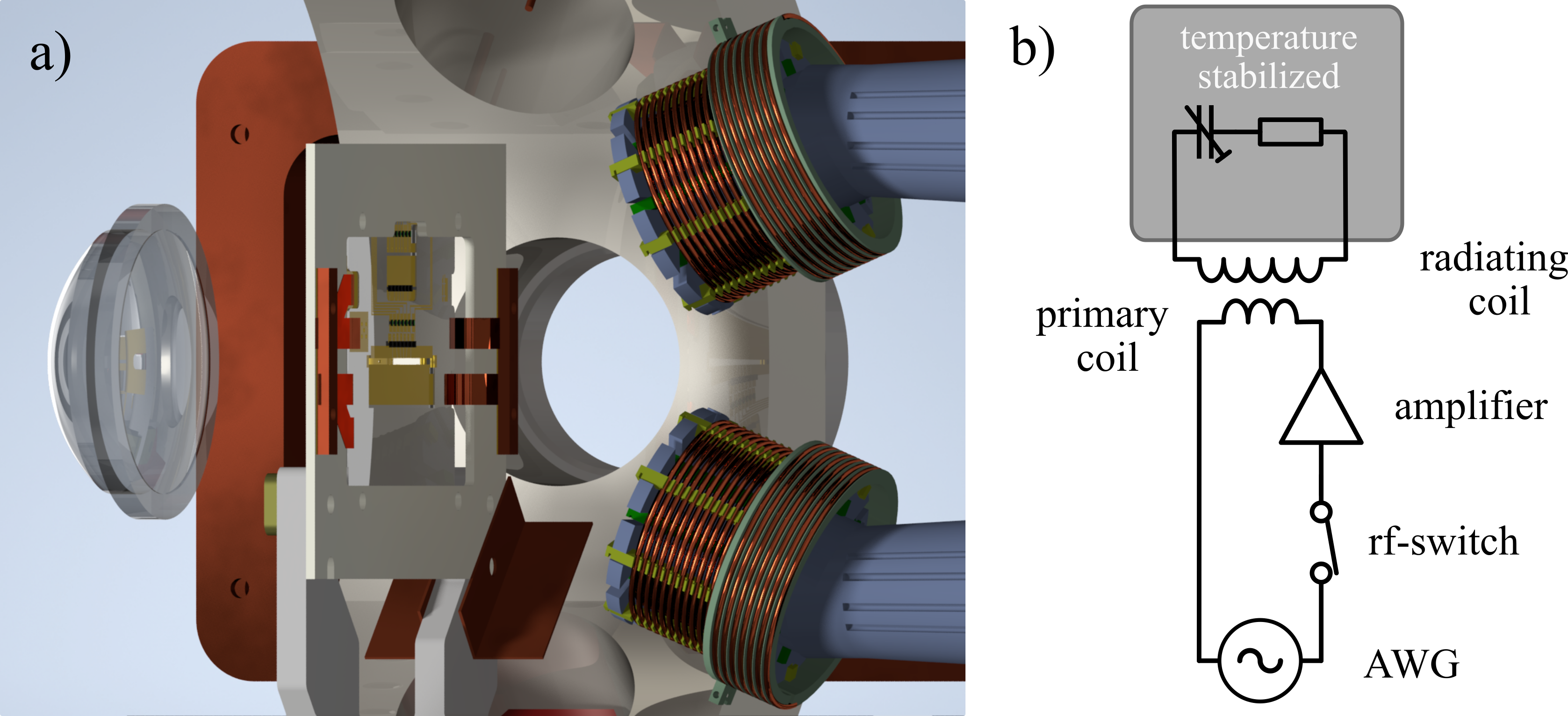
Figure 4: (a) CAD image of the CDD coil setup. RF magnetic field coils (right) for dressing the ${}^{2}\mathrm{S}_{1/2}$ and ${}^{2}\mathrm{D}_{5/2}$ are mounted at a distance of $d_{c}<$50\text{\,}\mathrm{mm}$$ to the Paul trap (centre). The aspheric lens (left) for imaging of the ion crystals has a distance of $d_{a}=$36.6\text{\,}\mathrm{mm}$$ to the trap centre. (b) Electronic schematic of the CDD drive.

The quality factor $Q_{S(D)}=14(30)$ of the coils is chosen as a compromise between large B-field amplitude and corresponding Rabi frequency for high Zeeman shift suppression (compare Eq. (14)) and minimal signal distortion by the coil’s transfer function. The resonance frequency $\omega_{0}(T)=\frac{1}{\sqrt{L(T)C(T)}}$ is temperature dependent. Therefore, the coil temperature increases by up to $10\text{\,}\mathrm{K}$ during operation depending on the applied rf power and the duty cycle of the rf-pulses within the experimental sequence. The circuit design includes a temperature-controlled base plate for the electronic components to avoid theses temperature-induced amplitude drifts. For passive temperature stability, the inductive part of the circuit is a copper coil held by an open, mesh-like 3D printed polylactide-part. This minimizes heat build-up during longer sequences. The holders are placed on translation stages and positioned in close proximity to the ion(s) inside an inverted viewport (see Fig. 4(a)).

IV.3 Experimental sequence

First, the ${}^{40}\mathrm{Ca}^{+}$-ion is Doppler-cooled close to the cooling limit of $T<$1\text{\,}\mathrm{mK}$$. The secular modes are then cooled to a mean motional phonon number of $\mkern 1.7mu\hbox{\vbox{\hrule height=0.4pt\kern 1.29167pt\hbox{\kern 0.0pt$\mkern-1.7mun\mkern-1.7mu$\kern 0.0pt}}}\mkern 1.7mu\lesssim 0.2$ by electromagnetically-induced-transparency cooling (Morigi et al., 2000; Roos et al., 2000; Scharnhorst et al., 2018) to reduce the second-order Doppler shift. After state preparation into the ${}^{2}\mathrm{S}_{1/2},\mathrm{m}=-1/2$ level by optical pumping with an axial $\sigma^{-}$ polarised $397\text{\,}\mathrm{nm}$ beam, the CDD sequence starts.

A frequency and amplitude ramp is applied, realizing a rapid adiabatic passage (Wunderlich et al., 2007), to avoid populating nearby dressed states by abrupt switching of the S-drive-coils. By choosing the sweep direction, the population is transferred to the $\mkern 1.7mu\hbox{\vbox{\hrule height=0.4pt\kern 1.29167pt\hbox{\kern 0.0pt$\mkern-1.7mum\mkern-1.7mu$\kern 0.0pt}}}\mkern 1.7mu=-\frac{1}{2}$ or $\mkern 1.7mu\hbox{\vbox{\hrule height=0.4pt\kern 1.29167pt\hbox{\kern 0.0pt$\mkern-1.7mum\mkern-1.7mu$\kern 0.0pt}}}\mkern 1.7mu=\frac{1}{2}$ dressed states with success probability of $P>98\,\%$. After this initial switch-on sequence, the S & D rf-drives are applied continuously together with a spectroscopy $729\text{\,}\mathrm{nm}$ pulse.

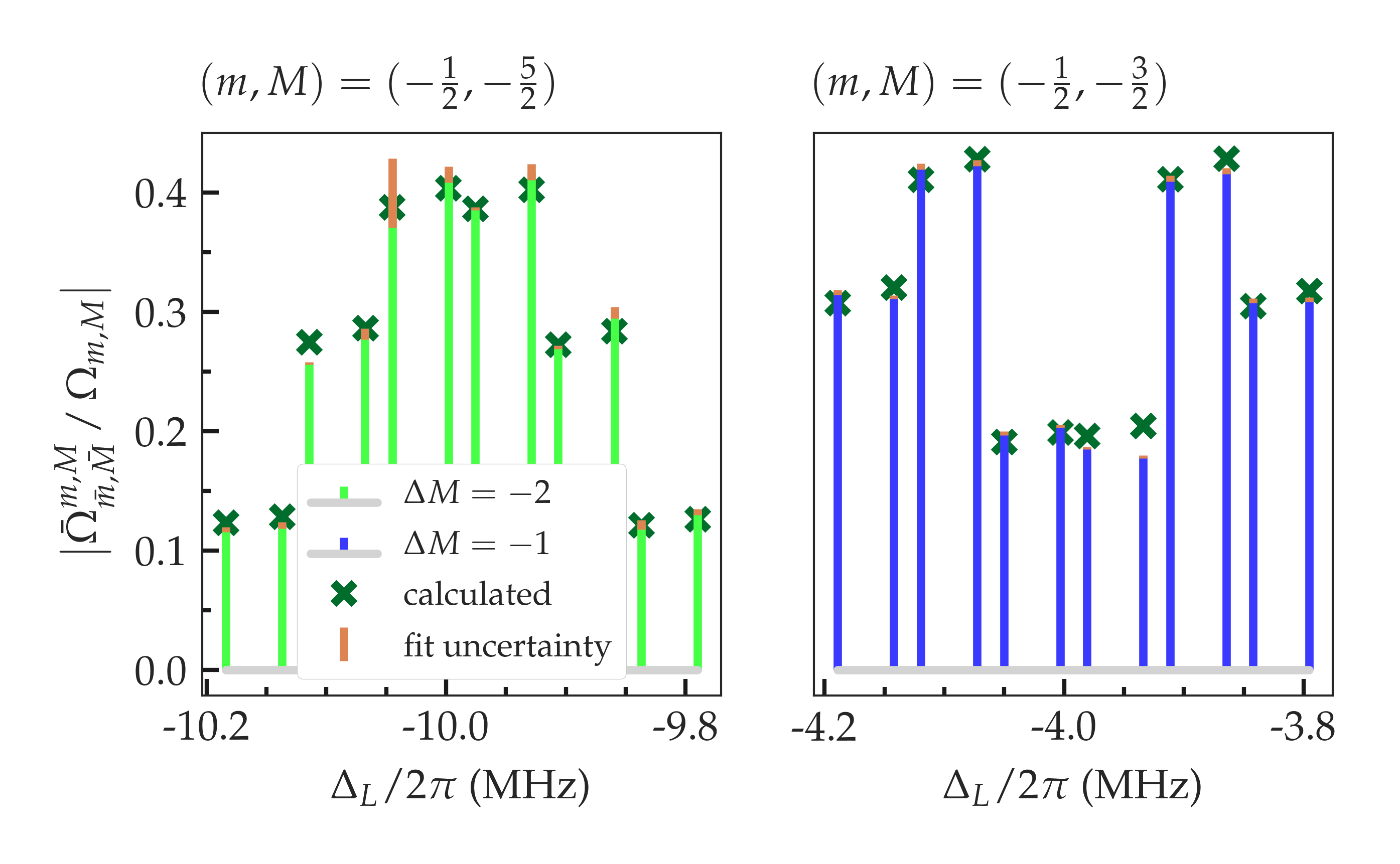
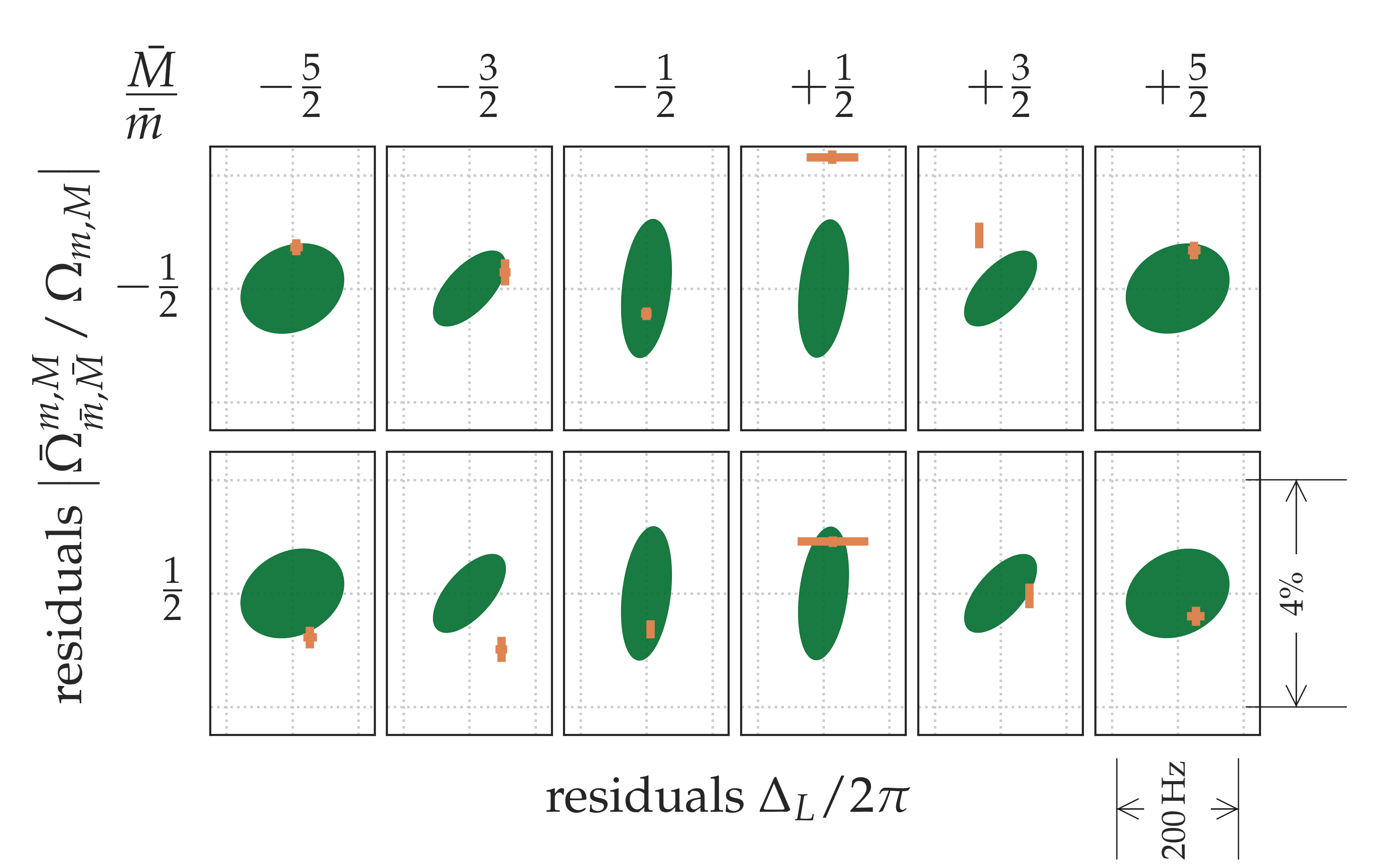
Figure 5: Comparison between experimental and theoretical coupling strengths and resonance frequencies for singly-dressed ${}^{40}\mathrm{Ca}^{+}$. (a) Relative optical coupling strength of two 1^st-stage ensembles with $\theta_{S(D)}=\pi/2$. Pulse length spectroscopy was used to determine the optical coupling strength of each transition. The relative coupling strength of the $729\text{\,}\mathrm{n}\mathrm{m}$ beam with respect to the associated Zeeman transition is plotted against the frequency offset from the zero B-field transition frequency. (b) Residuals for the $m=-\frac{1}{2},\,M=-\frac{3}{2}$ ensemble. The measured transitions values (orange) and the calculated (dark green) are compared. For the calculated uncertainty region, a fractional driving strength uncertainty of $\frac{\Delta\Omega_{i}}{\Omega_{i}}=4\times 10^{-4}$ and B-field uncertainty of $\Delta B_{0}=$60\text{\,}\mathrm{nT}$$ is assumed. For the measured data, only the fitting uncertainty was taken into account.

The dressed states resonances are addressed by their frequency detuning from the field-free $S_{1/2}\rightarrow D_{5/2}$ transition by the $729\text{\,}\mathrm{n}\mathrm{m}$ laser. If the optical coupling is much weaker than the rf-coupling ($\Omega_{m,M}\ll\mkern 1.7mu\hbox{\vbox{\hrule height=0.4pt\kern 1.29167pt\hbox{\kern 0.0pt$\mkern-1.7mu\omega\mkern-1.7mu$\kern 0.0pt}}}\mkern 1.7mu^{s,d}$), the dressed system’s Eigenstates are quasi-static with respect to the laser interaction. We have performed scans across the dressed state resonances to determine their frequency and on-resonance Rabi flopping to determine their coupling strength (compare appendix D).

For the prediction of the transition energies and coupling strengths of the dressed system adequate knowledge of the experimental parameters is crucial. The frequencies $\omega_{i}$ of the driving fields can be chosen with high precision, but the coupling strengths $\Omega_{i}$ must be determined experimentally via the splitting of the dressed states $\tilde{\omega}_{0}^{i}$. Therefore, resonance frequencies of four CDD transitions with opposing    $\mkern-1.7mum\mkern-1.7mu$   and    $\mkern-1.7muM\mkern-1.7mu$   are measured. With knowledge of these parameters the resonance frequencies and relative optical couplings of all 12 1^st-stage transitions per Zeeman-level can be determined (see Eq. (25) and (24)). In figure 5 the comparison of the measured and calculated optical coupling strengths for transitions from the $m=-\frac{1}{2}$ mainfold to the $M=-\frac{5}{2}$ and $M=-\frac{3}{2}$ manifolds are compared. The Rabi frequencies of the CDD states are normalized to the underlying bare Zeeman transition. The theoretical predictions are in good agreement with the measured transition frequencies and relative optical coupling strengths. Deviations arise from calibration imperfections and thermally induced drive strength fluctuations in combination with a drifting offset magnetic field. Equation. (24) predicts scaling of each CDD manifold with the underlying bare Zeeman transition. This was qualitatively confirmed by using different beam propagation directions. Especially, strict vanishing of dressed states together with an underlying bare Zeeman transitions with vanishing optical coupling (e.g. $|\Delta M|\neq 1$ for axial interrogation) was also confirmed.

V Mølmer-Sørensen gates.

We proceed to discuss the feasibility of executing a quantum gate on qubits defined by dressed states. Optical clocks based on entangled particles can provide a stability gain with the ion number $N$ over the standard quantum limit $\sigma_{y}\propto 1/\sqrt{N}\rightarrow 1/N$, the so-called Heisenberg limit (Leibfried et al., 2004; Kessler et al., 2014; Nichol et al., 2022). Therefore, suitably entangled states pose a promising way towards fast averaging ion clocks, even with moderate ion number (Schulte et al., 2020). For performing e.g. a Mølmer-Sørensen (MS) gate Häffner et al. (2008), this requires to drive sideband transitions off-resonantly in a way which is compatible with the dressing procedure explained in the previous sections.

We consider first a monochromatic driving field tuned close to one of the sideband transitions. In first order Lamb-Dicke expansion, the laser-ion interaction in the laboratory frame bare basis is James (1998)

$$V^{\mathrm{LF}}_{E2} =\mathrm{i}\sum_{m,M}\Bigl{\{}\Omega_{mM}\outerproduct{M}{m}\mathrm{e}^{-\mathrm{i}\Delta_{L}t}$$

$$\quad\times\left(1+\mathrm{i}\bar{\eta}\quantity(\hat{a}\mathrm{e}^{-\mathrm{i}\nu t}+\hat{a}^{\dagger}\mathrm{e}^{\mathrm{i}\nu t})\right)-\mathrm{h.c.}\Bigr{\}}.$$ (26)

Here $\bar{\eta}$ is the effective Lamb Dicke parameter, for which we assume $\bar{\eta}\ll 1$, and $\hat{a}$ and $\hat{a}^{\dagger}$ are creation/annhilation operators referring to one of the normal motional modes of the crystal. The laser detuning from the carrier transition in the bare basis is $\Delta_{L}$.

As an example, we consider the case where the detuning is chosen close to the red sideband of one of the transitions in the doubly dressed basis characterized by the set of quantum numbers $(m,M,\mkern 1.7mu\hbox{\vbox{\hrule height=0.4pt\kern 1.29167pt\hbox{\kern 0.0pt$\mkern-1.7mum\mkern-1.7mu$\kern 0.0pt}}}\mkern 1.7mu,\mkern 1.7mu\hbox{\vbox{\hrule height=0.4pt\kern 1.29167pt\hbox{\kern 0.0pt$\mkern-1.7muM\mkern-1.7mu$\kern 0.0pt}}}\mkern 1.7mu,\mkern 2.0mu\hbox{\vbox{\hrule height=0.4pt\kern 0.86108pt\hbox{\kern 0.0pt$\mkern-2.0mu\mkern 2.0mu\hbox{\vbox{\hrule height=0.4pt\kern 1.29167pt\hbox{\kern 0.0pt$\mkern-2.0mum\mkern-2.0mu$\kern 0.0pt}}}\mkern 2.0mu\mkern-2.0mu$\kern 0.0pt}}}\mkern 2.0mu,\mkern 2.0mu\hbox{\vbox{\hrule height=0.4pt\kern 0.86108pt\hbox{\kern 0.0pt$\mkern-2.0mu\mkern 2.0mu\hbox{\vbox{\hrule height=0.4pt\kern 1.29167pt\hbox{\kern 0.0pt$\mkern-2.0muM\mkern-2.0mu$\kern 0.0pt}}}\mkern 2.0mu\mkern-2.0mu$\kern 0.0pt}}}\mkern 2.0mu)$. This means, the detuning $\Delta_{L}$ satisfies

$$\Delta^{mM,\scriptsize{\mkern 2.0mu\hbox{\vbox{\hrule height=0.4pt\kern 0.90417pt\hbox{\kern 0.0pt$\mkern-2.0mum\mkern-2.0mu$\kern 0.0pt}}}\mkern 2.0mu}\mkern 1.7mu\hbox{\vbox{\hrule height=0.4pt\kern 0.90417pt\hbox{\kern 0.0pt$\mkern-1.7muM\mkern-1.7mu$\kern 0.0pt}}}\mkern 1.7mu}_{\scriptsize{\mkern 2.0mu\hbox{\vbox{\hrule height=0.4pt\kern 0.60275pt\hbox{\kern 0.0pt$\mkern-2.0mu\scriptsize{\mkern 2.0mu\hbox{\vbox{\hrule height=0.4pt\kern 0.90417pt\hbox{\kern 0.0pt$\mkern-2.0mum\mkern-2.0mu$\kern 0.0pt}}}\mkern 2.0mu}\mkern-2.0mu$\kern 0.0pt}}}\mkern 2.0mu}\scriptsize{\mkern 2.0mu\hbox{\vbox{\hrule height=0.4pt\kern 0.60275pt\hbox{\kern 0.0pt$\mkern-2.0mu\scriptsize{\mkern 2.0mu\hbox{\vbox{\hrule height=0.4pt\kern 0.90417pt\hbox{\kern 0.0pt$\mkern-2.0muM\mkern-2.0mu$\kern 0.0pt}}}\mkern 2.0mu}\mkern-2.0mu$\kern 0.0pt}}}\mkern 2.0mu}}+\nu=\delta,$$ (27)

where $\Delta^{mM,\scriptsize{\mkern 2.0mu\hbox{\vbox{\hrule height=0.4pt\kern 0.90417pt\hbox{\kern 0.0pt$\mkern-2.0mum\mkern-2.0mu$\kern 0.0pt}}}\mkern 2.0mu}\mkern 1.7mu\hbox{\vbox{\hrule height=0.4pt\kern 0.90417pt\hbox{\kern 0.0pt$\mkern-1.7muM\mkern-1.7mu$\kern 0.0pt}}}\mkern 1.7mu}_{\scriptsize{\mkern 2.0mu\hbox{\vbox{\hrule height=0.4pt\kern 0.60275pt\hbox{\kern 0.0pt$\mkern-2.0mu\scriptsize{\mkern 2.0mu\hbox{\vbox{\hrule height=0.4pt\kern 0.90417pt\hbox{\kern 0.0pt$\mkern-2.0mum\mkern-2.0mu$\kern 0.0pt}}}\mkern 2.0mu}\mkern-2.0mu$\kern 0.0pt}}}\mkern 2.0mu}\scriptsize{\mkern 2.0mu\hbox{\vbox{\hrule height=0.4pt\kern 0.60275pt\hbox{\kern 0.0pt$\mkern-2.0mu\scriptsize{\mkern 2.0mu\hbox{\vbox{\hrule height=0.4pt\kern 0.90417pt\hbox{\kern 0.0pt$\mkern-2.0muM\mkern-2.0mu$\kern 0.0pt}}}\mkern 2.0mu}\mkern-2.0mu$\kern 0.0pt}}}\mkern 2.0mu}}$ is given in Eq. (III.1), and $\delta$ is the detuning from the sideband transition (aka Mølmer-Sørensen detuning). In a rotating wave approximation with respect to all other terms, the Hamiltonian for a red sideband (rsb) transition becomes

$$V^{\mathrm{DB}}_{rsb}\approx -\bar{\eta}\Omega\outerproduct*{\mkern 2.0mu\hbox{\vbox{\hrule height=0.4pt\kern 0.86108pt\hbox{\kern 0.0pt$\mkern-2.0mu\mkern 2.0mu\hbox{\vbox{\hrule height=0.4pt\kern 1.29167pt\hbox{\kern 0.0pt$\mkern-2.0muM\mkern-2.0mu$\kern 0.0pt}}}\mkern 2.0mu\mkern-2.0mu$\kern 0.0pt}}}\mkern 2.0mu}{\mkern 2.0mu\hbox{\vbox{\hrule height=0.4pt\kern 0.86108pt\hbox{\kern 0.0pt$\mkern-2.0mu\mkern 2.0mu\hbox{\vbox{\hrule height=0.4pt\kern 1.29167pt\hbox{\kern 0.0pt$\mkern-2.0mum\mkern-2.0mu$\kern 0.0pt}}}\mkern 2.0mu\mkern-2.0mu$\kern 0.0pt}}}\mkern 2.0mu}\hat{a}\mathrm{e}^{-\mathrm{i}\delta t}+h.c.,$$ (28)

where $\Omega=\bar{\Omega}^{mM,\scriptsize{\mkern 2.0mu\hbox{\vbox{\hrule height=0.4pt\kern 0.90417pt\hbox{\kern 0.0pt$\mkern-2.0mum\mkern-2.0mu$\kern 0.0pt}}}\mkern 2.0mu}\scriptsize{\mkern 2.0mu\hbox{\vbox{\hrule height=0.4pt\kern 0.90417pt\hbox{\kern 0.0pt$\mkern-2.0muM\mkern-2.0mu$\kern 0.0pt}}}\mkern 2.0mu}}_{\scriptsize{\mkern 2.0mu\hbox{\vbox{\hrule height=0.4pt\kern 0.60275pt\hbox{\kern 0.0pt$\mkern-2.0mu\scriptsize{\mkern 2.0mu\hbox{\vbox{\hrule height=0.4pt\kern 0.90417pt\hbox{\kern 0.0pt$\mkern-2.0mum\mkern-2.0mu$\kern 0.0pt}}}\mkern 2.0mu}\mkern-2.0mu$\kern 0.0pt}}}\mkern 2.0mu}\scriptsize{\mkern 2.0mu\hbox{\vbox{\hrule height=0.4pt\kern 0.60275pt\hbox{\kern 0.0pt$\mkern-2.0mu\scriptsize{\mkern 2.0mu\hbox{\vbox{\hrule height=0.4pt\kern 0.90417pt\hbox{\kern 0.0pt$\mkern-2.0muM\mkern-2.0mu$\kern 0.0pt}}}\mkern 2.0mu}\mkern-2.0mu$\kern 0.0pt}}}\mkern 2.0mu}}$, as given in Eq. (III.1). Given that $\mkern 1.7mu\hbox{\vbox{\hrule height=0.4pt\kern 0.86108pt\hbox{\kern 0.0pt$\mkern-1.7mu\mkern 1.7mu\hbox{\vbox{\hrule height=0.4pt\kern 1.29167pt\hbox{\kern 0.0pt$\mkern-1.7mu\omega\mkern-1.7mu$\kern 0.0pt}}}\mkern 1.7mu\mkern-1.7mu$\kern 0.0pt}}}\mkern 1.7mu_{0}^{d}$ will be the smallest frequency scale in the comb of frequencies induced by the dressing fields, the closest neighbouring transitions will be $\Delta^{mM,\scriptsize{\mkern 2.0mu\hbox{\vbox{\hrule height=0.4pt\kern 0.90417pt\hbox{\kern 0.0pt$\mkern-2.0mum\mkern-2.0mu$\kern 0.0pt}}}\mkern 2.0mu}\mkern 1.7mu\hbox{\vbox{\hrule height=0.4pt\kern 0.90417pt\hbox{\kern 0.0pt$\mkern-1.7muM\mkern-1.7mu$\kern 0.0pt}}}\mkern 1.7mu}_{\scriptsize{\mkern 2.0mu\hbox{\vbox{\hrule height=0.4pt\kern 0.60275pt\hbox{\kern 0.0pt$\mkern-2.0mu\scriptsize{\mkern 2.0mu\hbox{\vbox{\hrule height=0.4pt\kern 0.90417pt\hbox{\kern 0.0pt$\mkern-2.0mum\mkern-2.0mu$\kern 0.0pt}}}\mkern 2.0mu}\mkern-2.0mu$\kern 0.0pt}}}\mkern 2.0mu}\scriptsize{\mkern 2.0mu\hbox{\vbox{\hrule height=0.4pt\kern 0.60275pt\hbox{\kern 0.0pt$\mkern-2.0mu\scriptsize{\mkern 2.0mu\hbox{\vbox{\hrule height=0.4pt\kern 0.90417pt\hbox{\kern 0.0pt$\mkern-2.0muM\mkern-2.0mu$\kern 0.0pt}}}\mkern 2.0mu}\mkern-2.0mu$\kern 0.0pt}}}\mkern 2.0mu}\pm 1}$, which will be separated by $\mkern 1.7mu\hbox{\vbox{\hrule height=0.4pt\kern 0.86108pt\hbox{\kern 0.0pt$\mkern-1.7mu\mkern 1.7mu\hbox{\vbox{\hrule height=0.4pt\kern 1.29167pt\hbox{\kern 0.0pt$\mkern-1.7mu\omega\mkern-1.7mu$\kern 0.0pt}}}\mkern 1.7mu\mkern-1.7mu$\kern 0.0pt}}}\mkern 1.7mu_{0}^{d}$. We therefore require $\delta\ll\mkern 1.7mu\hbox{\vbox{\hrule height=0.4pt\kern 0.86108pt\hbox{\kern 0.0pt$\mkern-1.7mu\mkern 1.7mu\hbox{\vbox{\hrule height=0.4pt\kern 1.29167pt\hbox{\kern 0.0pt$\mkern-1.7mu\omega\mkern-1.7mu$\kern 0.0pt}}}\mkern 1.7mu\mkern-1.7mu$\kern 0.0pt}}}\mkern 1.7mu_{0}^{d}$ and $\absolutevalue*{\Omega}\ll\absolutevalue*{\mkern 1.7mu\hbox{\vbox{\hrule height=0.4pt\kern 0.86108pt\hbox{\kern 0.0pt$\mkern-1.7mu\mkern 1.7mu\hbox{\vbox{\hrule height=0.4pt\kern 1.29167pt\hbox{\kern 0.0pt$\mkern-1.7mu\omega\mkern-1.7mu$\kern 0.0pt}}}\mkern 1.7mu\mkern-1.7mu$\kern 0.0pt}}}\mkern 1.7mu_{0}^{d}}$ in applying the rotating wave approximation. For the blue sideband (bsb) one has instead

$$V^{\mathrm{DB}}_{bsb}\approx -\bar{\eta}\Omega\outerproduct*{\mkern 2.0mu\hbox{\vbox{\hrule height=0.4pt\kern 0.86108pt\hbox{\kern 0.0pt$\mkern-2.0mu\mkern 2.0mu\hbox{\vbox{\hrule height=0.4pt\kern 1.29167pt\hbox{\kern 0.0pt$\mkern-2.0muM\mkern-2.0mu$\kern 0.0pt}}}\mkern 2.0mu\mkern-2.0mu$\kern 0.0pt}}}\mkern 2.0mu}{\mkern 2.0mu\hbox{\vbox{\hrule height=0.4pt\kern 0.86108pt\hbox{\kern 0.0pt$\mkern-2.0mu\mkern 2.0mu\hbox{\vbox{\hrule height=0.4pt\kern 1.29167pt\hbox{\kern 0.0pt$\mkern-2.0mum\mkern-2.0mu$\kern 0.0pt}}}\mkern 2.0mu\mkern-2.0mu$\kern 0.0pt}}}\mkern 2.0mu}\hat{a}^{\dagger}\mathrm{e}^{-\mathrm{i}\delta t}+h.c.,$$ (29)

with $\Delta^{mM,\scriptsize{\mkern 2.0mu\hbox{\vbox{\hrule height=0.4pt\kern 0.90417pt\hbox{\kern 0.0pt$\mkern-2.0mum\mkern-2.0mu$\kern 0.0pt}}}\mkern 2.0mu}\mkern 1.7mu\hbox{\vbox{\hrule height=0.4pt\kern 0.90417pt\hbox{\kern 0.0pt$\mkern-1.7muM\mkern-1.7mu$\kern 0.0pt}}}\mkern 1.7mu}_{\scriptsize{\mkern 2.0mu\hbox{\vbox{\hrule height=0.4pt\kern 0.60275pt\hbox{\kern 0.0pt$\mkern-2.0mu\scriptsize{\mkern 2.0mu\hbox{\vbox{\hrule height=0.4pt\kern 0.90417pt\hbox{\kern 0.0pt$\mkern-2.0mum\mkern-2.0mu$\kern 0.0pt}}}\mkern 2.0mu}\mkern-2.0mu$\kern 0.0pt}}}\mkern 2.0mu}\scriptsize{\mkern 2.0mu\hbox{\vbox{\hrule height=0.4pt\kern 0.60275pt\hbox{\kern 0.0pt$\mkern-2.0mu\scriptsize{\mkern 2.0mu\hbox{\vbox{\hrule height=0.4pt\kern 0.90417pt\hbox{\kern 0.0pt$\mkern-2.0muM\mkern-2.0mu$\kern 0.0pt}}}\mkern 2.0mu}\mkern-2.0mu$\kern 0.0pt}}}\mkern 2.0mu}}-\nu=\delta$. For driving a MS gate, we require $\absolutevalue*{\Omega}\ll\absolutevalue*{\delta}$. Thus, the MS detuning, the effective sideband Rabi frequency and the smallest frequency split in the double-dressed basis must therefore satisfy a hierarchy of coupling strengths $\Omega\ll\delta\ll\mkern 1.7mu\hbox{\vbox{\hrule height=0.4pt\kern 0.86108pt\hbox{\kern 0.0pt$\mkern-1.7mu\mkern 1.7mu\hbox{\vbox{\hrule height=0.4pt\kern 1.29167pt\hbox{\kern 0.0pt$\mkern-1.7mu\omega\mkern-1.7mu$\kern 0.0pt}}}\mkern 1.7mu\mkern-1.7mu$\kern 0.0pt}}}\mkern 1.7mu_{0}^{d}$.

For a bi-chromatic field driving the red and the blue sideband transitions at the same time on a crystal of ions, the time evolution operator can be expressed in a Magnus expansion Magnus (1954)

$$U(t)=\mathrm{e}^{\sum_{j}\sigma_{x}^{(j)}\quantity(\alpha_{j}(t)a^{\dagger}-\alpha^{\star}(t)a)}\mathrm{e}^{-\mathrm{i}\sum_{j,n}\sigma_{x}^{(j)}\sigma_{x}^{(n)}\Phi(t)},$$ (30)

with the time-dependent displacement and the geometric phase

$$\alpha(t) =\frac{\Omega}{\delta}\quantity(\mathrm{e}^{-\mathrm{i}\delta t}-1), \Phi(t) =\frac{\Omega^{2}}{\delta}\left[t-\frac{1}{\delta}\sin\quantity(\delta t)\right],$$ (31)

respectively. Here we used the Pauli operator $\sigma_{x}=\outerproduct*{\mkern 2.0mu\hbox{\vbox{\hrule height=0.4pt\kern 0.86108pt\hbox{\kern 0.0pt$\mkern-2.0mu\mkern 2.0mu\hbox{\vbox{\hrule height=0.4pt\kern 1.29167pt\hbox{\kern 0.0pt$\mkern-2.0muM\mkern-2.0mu$\kern 0.0pt}}}\mkern 2.0mu\mkern-2.0mu$\kern 0.0pt}}}\mkern 2.0mu}{\mkern 2.0mu\hbox{\vbox{\hrule height=0.4pt\kern 0.86108pt\hbox{\kern 0.0pt$\mkern-2.0mu\mkern 2.0mu\hbox{\vbox{\hrule height=0.4pt\kern 1.29167pt\hbox{\kern 0.0pt$\mkern-2.0mum\mkern-2.0mu$\kern 0.0pt}}}\mkern 2.0mu\mkern-2.0mu$\kern 0.0pt}}}\mkern 2.0mu}+\outerproduct*{\mkern 2.0mu\hbox{\vbox{\hrule height=0.4pt\kern 0.86108pt\hbox{\kern 0.0pt$\mkern-2.0mu\mkern 2.0mu\hbox{\vbox{\hrule height=0.4pt\kern 1.29167pt\hbox{\kern 0.0pt$\mkern-2.0mum\mkern-2.0mu$\kern 0.0pt}}}\mkern 2.0mu\mkern-2.0mu$\kern 0.0pt}}}\mkern 2.0mu}{\mkern 2.0mu\hbox{\vbox{\hrule height=0.4pt\kern 0.86108pt\hbox{\kern 0.0pt$\mkern-2.0mu\mkern 2.0mu\hbox{\vbox{\hrule height=0.4pt\kern 1.29167pt\hbox{\kern 0.0pt$\mkern-2.0muM\mkern-2.0mu$\kern 0.0pt}}}\mkern 2.0mu\mkern-2.0mu$\kern 0.0pt}}}\mkern 2.0mu}$ and write $\sigma^{(j)}_{x}$ for the operator referring to the $j$-th ion ($j=1,\ldots,N$). For simplicity, we assumed that the sideband Rabi frequency is the same for all particles. In order to decouple the mode of motion in the end of the gate at time $T$, we require $\delta T=2n\pi$ for $n\in\mathds{N}$. For achieving a maximally entangling gate, we need $T\Omega^{2}/\delta=2\pi K$ for $K$ the number of loops executed in phase space.

Picking up the concrete example treated in the previous section, we can estimate the gate parameters. In view of $\Omega\ll\delta\ll\mkern 1.7mu\hbox{\vbox{\hrule height=0.4pt\kern 0.86108pt\hbox{\kern 0.0pt$\mkern-1.7mu\mkern 1.7mu\hbox{\vbox{\hrule height=0.4pt\kern 1.29167pt\hbox{\kern 0.0pt$\mkern-1.7mu\omega\mkern-1.7mu$\kern 0.0pt}}}\mkern 1.7mu\mkern-1.7mu$\kern 0.0pt}}}\mkern 1.7mu_{0}$, we assume $3\Omega_{s}=\delta=\mkern 1.7mu\hbox{\vbox{\hrule height=0.4pt\kern 0.86108pt\hbox{\kern 0.0pt$\mkern-1.7mu\mkern 1.7mu\hbox{\vbox{\hrule height=0.4pt\kern 1.29167pt\hbox{\kern 0.0pt$\mkern-1.7mu\omega\mkern-1.7mu$\kern 0.0pt}}}\mkern 1.7mu\mkern-1.7mu$\kern 0.0pt}}}\mkern 1.7mu_{0}/3$. Assuming $n=K=1$, we estimate a gate duration

$$T=2\pi\frac{\delta}{\Omega^{2}}=2\pi\frac{9}{\delta}=2\pi\frac{27}{\mkern 1.7mu\hbox{\vbox{\hrule height=0.4pt\kern 0.86108pt\hbox{\kern 0.0pt$\mkern-1.7mu\mkern 1.7mu\hbox{\vbox{\hrule height=0.4pt\kern 1.29167pt\hbox{\kern 0.0pt$\mkern-1.7mu\omega\mkern-1.7mu$\kern 0.0pt}}}\mkern 1.7mu\mkern-1.7mu$\kern 0.0pt}}}\mkern 1.7mu_{0}}\approx 3.375\mathrm{ms}.$$ (32)

While this will not be a competitive gate for quantum computing applications, it may well be sufficient for applications in ion clocks. For ion clocks the gate time has to be compared with the interrogation time which can be on the order of seconds. The extra time of the gate will add to the dark time of the interrogation scheme. We note that some of the conditions imposed on the parameters can be relaxed by exploiting the structure of the comb of frequencies induced by the dressing procedure.

VI Conclusions

In this article we developed a compact formalism to describe nested layers of continuous dynamical decoupling by rf dressing fields of ground and excited state Zeeman manifolds. We showed that two layers of dressing can be used to cancel linear Zeeman shifts and electric-quadrupole shifts, and established criteria for which shift to cancel at what layer of dressing. Our main result concerns the description of quadrupole laser-ion interaction in the basis of doubly-dressed states. We characterized the comb of transition frequencies induced by the dressing and expressed the effective Rabi and the transitions frequencies in terms of a set of quantum numbers, which allowed us also to identify the relevant selection rules for these transitions. We addressed the rotating wave approximations and the cross-field effect by treating them in an approximate manner using a Magnus expansion, and showed that both can be effectively interpreted as a shift of the Zeeman splitting for the Zeeman manifolds. With this correction, theoretical predictions are in excellent agreement with experimental data for the quadrupole transitions $S_{1/2}\rightarrow D_{5/2}$ in ${}^{40}\mathrm{Ca}^{+}$. We used our insights to estimate the feasibility of executing MS-gates on the level of the doubly-dressed basis, showing gate times on the order of milliseconds, which is in principle sufficient for use in ion clocks. Faster gates are possible with only one layer of dressing, at the expense of becoming more sensitive to either Zeeman or electric-quadrupole shifts. Gates can be further optimized by exploiting the selection rules and the specific structure of the comb of frequencies induced by the dressing.

Appendix A Magnetic field fluctuations and Quadrupole shift in the interaction picture

To calculate the energy shift of the bare states created through magnetic field fluctuations, Eq. (13), in the interaction picture, the changes of the spin vectors for the different transformations must be taken into account.

In a RWA one has $\mathcal{R}_{\mathbb{z}}(\omega t)\mathbf{S}=S_{z}\mathbb{e}_{z}$, therefore, applying the rotation and going to an interaction picture for one layer with a general direction of rotation $\mathbb{n}=\cos\varphi\mathbb{e}_{x}+\sin\varphi\mathbb{e}_{y}$, we obtain

$$\mathcal{R}_{\mathbb{z}}(\omega t)\mathcal{R}_{\mathbb{n}}(\theta)S_{z}$$

$$=\cos\theta S_{z}+\frac{\mathrm{i}}{2}\sin\theta\left(e^{\mathrm{i}t(\omega+\varphi)}S_{+}-e^{-\mathrm{i}t(\omega+\varphi)}S_{-}\right)$$

$$\simeq\cos\theta S_{z}.$$ (33)

The RWA drops all the terms oscillating at frequency $\omega+\varphi$. This can be applied for the two dressing layers, recovering the result of Eq. (14).

The quadrupole operator, defined by $Q_{ij}=\frac{3}{2}\left(S_{i}S_{j}+S_{j}S_{i}\right)-S\left(S+1\right)\mathds{1}$, becomes in a RWA

$$\mathcal{R}_{\mathbb{z}}(\omega t)Q \simeq\frac{3}{2}\begin{pmatrix}S_{x}^{2}+S_{y}^{2}&0&0\\ 0&S_{x}^{2}+S_{y}^{2}&0\\ 0&0&2S_{z}^{2}\end{pmatrix}-S(S+1)\mathds{1}$$

$$=\frac{S(S+1)-3S_{z}^{2}}{2}\begin{pmatrix}1&0&0\\ 0&1&0\\ 0&0&-2\end{pmatrix}.$$ (34)

The latter expression is useful for evaluating the quadrupole shift. This is further simplified when using the Laplace equation $F_{xx}+F_{yy}+F_{zz}=0$ in the quadrupole shift Hamiltonian

$$\mathcal{R}_{\mathbb{z}}(\omega t)V_{Q}^{\mathrm{LF}} =\Tr{\mathcal{R}_{\mathbb{z}}(\omega t)[Q]F}$$

$$\simeq\frac{3F_{zz}}{2}\left(3S_{z}^{2}-S(S+1)\right).$$ (35)

Thus, in the first layer of dressing one has to evaluate

$$\mathcal{R}_{\mathbb{z}}(\omega t)\mathcal{R}_{\mathbb{n}}(\theta)S^{2}_{z}$$

$$=\quantity[\cos\theta S_{z}+\frac{\mathrm{i}}{2}\sin\theta\left(e^{\mathrm{i}t(\omega+\varphi)}S_{+}-e^{-\mathrm{i}t(\omega+\varphi)}S_{-}\right)]^{2}$$

$$\simeq\cos^{2}\theta S^{2}_{z}+\frac{\sin^{2}\theta}{4}(S_{+}S_{-}+S_{-}S_{+})$$

$$=\frac{\sin^{2}\theta}{2}S(S+1)-\frac{1-3\cos^{2}\theta}{2}S_{z}^{2}$$ (36)

Iterating this expression another time yields Eq. (16).

Appendix B Effective Rabi frequency in the doubled dressed basis

For evaluating the laser-ion interaction in the dressed basis the expression

$$\matrixelement*{\mkern 2.0mu\hbox{\vbox{\hrule height=0.4pt\kern 0.86108pt\hbox{\kern 0.0pt$\mkern-2.0mu\mkern 2.0mu\hbox{\vbox{\hrule height=0.4pt\kern 1.29167pt\hbox{\kern 0.0pt$\mkern-2.0muM\mkern-2.0mu$\kern 0.0pt}}}\mkern 2.0mu\mkern-2.0mu$\kern 0.0pt}}}\mkern 2.0mu}{\mathcal{D}^{\mathrm{s}}\otimes\mathcal{D}^{\mathrm{d}}\quantity\big[\outerproduct{M}{m}]}{\mkern 2.0mu\hbox{\vbox{\hrule height=0.4pt\kern 0.86108pt\hbox{\kern 0.0pt$\mkern-2.0mu\mkern 2.0mu\hbox{\vbox{\hrule height=0.4pt\kern 1.29167pt\hbox{\kern 0.0pt$\mkern-2.0mum\mkern-2.0mu$\kern 0.0pt}}}\mkern 2.0mu\mkern-2.0mu$\kern 0.0pt}}}\mkern 2.0mu}=\mathcal{U}^{\mathrm{d}}_{\scriptsize{\mkern 2.0mu\hbox{\vbox{\hrule height=0.4pt\kern 0.60275pt\hbox{\kern 0.0pt$\mkern-2.0mu\scriptsize{\mkern 2.0mu\hbox{\vbox{\hrule height=0.4pt\kern 0.90417pt\hbox{\kern 0.0pt$\mkern-2.0muM\mkern-2.0mu$\kern 0.0pt}}}\mkern 2.0mu}\mkern-2.0mu$\kern 0.0pt}}}\mkern 2.0mu}M}(t)\quantity(\mathcal{U}^{\mathrm{s}}_{\scriptsize{\mkern 2.0mu\hbox{\vbox{\hrule height=0.4pt\kern 0.60275pt\hbox{\kern 0.0pt$\mkern-2.0mu\scriptsize{\mkern 2.0mu\hbox{\vbox{\hrule height=0.4pt\kern 0.90417pt\hbox{\kern 0.0pt$\mkern-2.0mum\mkern-2.0mu$\kern 0.0pt}}}\mkern 2.0mu}\mkern-2.0mu$\kern 0.0pt}}}\mkern 2.0mu}m}(t))^{*}$$ (37)

is used, with

$$\mathcal{U}^{\mathrm{d}}_{\scriptsize{\mkern 2.0mu\hbox{\vbox{\hrule height=0.4pt\kern 0.60275pt\hbox{\kern 0.0pt$\mkern-2.0mu\scriptsize{\mkern 2.0mu\hbox{\vbox{\hrule height=0.4pt\kern 0.90417pt\hbox{\kern 0.0pt$\mkern-2.0muM\mkern-2.0mu$\kern 0.0pt}}}\mkern 2.0mu}\mkern-2.0mu$\kern 0.0pt}}}\mkern 2.0mu}M}(t)=$$

$$\matrixelement*{\mkern 2.0mu\hbox{\vbox{\hrule height=0.4pt\kern 0.86108pt\hbox{\kern 0.0pt$\mkern-2.0mu\mkern 2.0mu\hbox{\vbox{\hrule height=0.4pt\kern 1.29167pt\hbox{\kern 0.0pt$\mkern-2.0muM\mkern-2.0mu$\kern 0.0pt}}}\mkern 2.0mu\mkern-2.0mu$\kern 0.0pt}}}\mkern 2.0mu}{U_{\mathbb{z}}(\mkern 1.7mu\hbox{\vbox{\hrule height=0.4pt\kern 0.86108pt\hbox{\kern 0.0pt$\mkern-1.7mu\mkern 1.7mu\hbox{\vbox{\hrule height=0.4pt\kern 1.29167pt\hbox{\kern 0.0pt$\mkern-1.7mu\omega\mkern-1.7mu$\kern 0.0pt}}}\mkern 1.7mu\mkern-1.7mu$\kern 0.0pt}}}\mkern 1.7mu_{0}^{\mathrm{d}}t)U_{\mathbb{n^{\mathrm{d}}_{\text{2}}}}(\theta_{2}^{\mathrm{d}})U_{\mathbb{z}}(\omega^{\mathrm{d}}_{2}t)U_{\mathbb{n^{\mathrm{d}}_{\text{1}}}}(\theta_{1}^{\mathrm{d}})U_{\mathbb{z}}(\omega^{\mathrm{d}}_{1}t)}{M}$$ (38)

and equivalently for $\mathcal{U}^{\mathrm{s}}_{\scriptsize{\mkern 2.0mu\hbox{\vbox{\hrule height=0.4pt\kern 0.60275pt\hbox{\kern 0.0pt$\mkern-2.0mu\scriptsize{\mkern 2.0mu\hbox{\vbox{\hrule height=0.4pt\kern 0.90417pt\hbox{\kern 0.0pt$\mkern-2.0mum\mkern-2.0mu$\kern 0.0pt}}}\mkern 2.0mu}\mkern-2.0mu$\kern 0.0pt}}}\mkern 2.0mu}m}(t)$ with $\mathrm{d}\leftrightarrow\mathrm{s}$ and $\mkern 2.0mu\hbox{\vbox{\hrule height=0.4pt\kern 0.86108pt\hbox{\kern 0.0pt$\mkern-2.0mu\mkern 2.0mu\hbox{\vbox{\hrule height=0.4pt\kern 1.29167pt\hbox{\kern 0.0pt$\mkern-2.0muM\mkern-2.0mu$\kern 0.0pt}}}\mkern 2.0mu\mkern-2.0mu$\kern 0.0pt}}}\mkern 2.0mu,M\leftrightarrow\mkern 2.0mu\hbox{\vbox{\hrule height=0.4pt\kern 0.86108pt\hbox{\kern 0.0pt$\mkern-2.0mu\mkern 2.0mu\hbox{\vbox{\hrule height=0.4pt\kern 1.29167pt\hbox{\kern 0.0pt$\mkern-2.0mum\mkern-2.0mu$\kern 0.0pt}}}\mkern 2.0mu\mkern-2.0mu$\kern 0.0pt}}}\mkern 2.0mu,m$. As an example we will evaluate the matrix elements for the $\differential$-states.

$$\matrixelement*{\mkern 2.0mu\hbox{\vbox{\hrule height=0.4pt\kern 0.86108pt\hbox{\kern 0.0pt$\mkern-2.0mu\mkern 2.0mu\hbox{\vbox{\hrule height=0.4pt\kern 1.29167pt\hbox{\kern 0.0pt$\mkern-2.0muM\mkern-2.0mu$\kern 0.0pt}}}\mkern 2.0mu\mkern-2.0mu$\kern 0.0pt}}}\mkern 2.0mu}{U_{\mathbb{z}}(\mkern 1.7mu\hbox{\vbox{\hrule height=0.4pt\kern 0.86108pt\hbox{\kern 0.0pt$\mkern-1.7mu\mkern 1.7mu\hbox{\vbox{\hrule height=0.4pt\kern 1.29167pt\hbox{\kern 0.0pt$\mkern-1.7mu\omega\mkern-1.7mu$\kern 0.0pt}}}\mkern 1.7mu\mkern-1.7mu$\kern 0.0pt}}}\mkern 1.7mu_{0}t)U_{\mathbb{n_{\text{2}}}}(\theta_{2})U_{\mathbb{z}}(\omega_{2}t)U_{\mathbb{n_{\text{1}}}}(\theta_{1})U_{\mathbb{z}}(\omega_{1}t)}{M}$$

$$=\sum_{\scriptsize{\mkern 2.0mu\hbox{\vbox{\hrule height=0.4pt\kern 0.90417pt\hbox{\kern 0.0pt$\mkern-2.0muM\mkern-2.0mu$\kern 0.0pt}}}\mkern 2.0mu}}\matrixelement*{\mkern 2.0mu\hbox{\vbox{\hrule height=0.4pt\kern 0.86108pt\hbox{\kern 0.0pt$\mkern-2.0mu\mkern 2.0mu\hbox{\vbox{\hrule height=0.4pt\kern 1.29167pt\hbox{\kern 0.0pt$\mkern-2.0muM\mkern-2.0mu$\kern 0.0pt}}}\mkern 2.0mu\mkern-2.0mu$\kern 0.0pt}}}\mkern 2.0mu}{U_{\mathbb{n_{\text{2}}}}(\theta_{2})}{\mkern 1.7mu\hbox{\vbox{\hrule height=0.4pt\kern 1.29167pt\hbox{\kern 0.0pt$\mkern-1.7muM\mkern-1.7mu$\kern 0.0pt}}}\mkern 1.7mu}\matrixelement*{\mkern 1.7mu\hbox{\vbox{\hrule height=0.4pt\kern 1.29167pt\hbox{\kern 0.0pt$\mkern-1.7muM\mkern-1.7mu$\kern 0.0pt}}}\mkern 1.7mu}{U_{\mathbb{n_{\text{1}}}}(\theta_{1})}{M}$$

$$\quad\times\mathrm{e}^{\mathrm{i}\quantity(\scriptsize{\mkern 2.0mu\hbox{\vbox{\hrule height=0.4pt\kern 0.60275pt\hbox{\kern 0.0pt$\mkern-2.0mu\scriptsize{\mkern 2.0mu\hbox{\vbox{\hrule height=0.4pt\kern 0.90417pt\hbox{\kern 0.0pt$\mkern-2.0muM\mkern-2.0mu$\kern 0.0pt}}}\mkern 2.0mu}\mkern-2.0mu$\kern 0.0pt}}}\mkern 2.0mu}\mkern 1.7mu\hbox{\vbox{\hrule height=0.4pt\kern 0.60275pt\hbox{\kern 0.0pt$\mkern-1.7mu\mkern 1.7mu\hbox{\vbox{\hrule height=0.4pt\kern 0.90417pt\hbox{\kern 0.0pt$\mkern-1.7mu\omega\mkern-1.7mu$\kern 0.0pt}}}\mkern 1.7mu\mkern-1.7mu$\kern 0.0pt}}}\mkern 1.7mu_{0}+\scriptsize{\mkern 2.0mu\hbox{\vbox{\hrule height=0.4pt\kern 0.90417pt\hbox{\kern 0.0pt$\mkern-2.0muM\mkern-2.0mu$\kern 0.0pt}}}\mkern 2.0mu}\omega_{2}+M\omega_{1})t},$$ (39)

where we used the expansion of the identity $\mathds{1}=\sum_{\scriptsize{\mkern 2.0mu\hbox{\vbox{\hrule height=0.4pt\kern 0.90417pt\hbox{\kern 0.0pt$\mkern-2.0muM\mkern-2.0mu$\kern 0.0pt}}}\mkern 2.0mu}}\outerproduct*{\mkern 1.7mu\hbox{\vbox{\hrule height=0.4pt\kern 1.29167pt\hbox{\kern 0.0pt$\mkern-1.7muM\mkern-1.7mu$\kern 0.0pt}}}\mkern 1.7mu}{\mkern 1.7mu\hbox{\vbox{\hrule height=0.4pt\kern 1.29167pt\hbox{\kern 0.0pt$\mkern-1.7muM\mkern-1.7mu$\kern 0.0pt}}}\mkern 1.7mu}$. Finally, the remaining matrix elements of the unitary matrices corresponding to the rotations of the quantization axis are

$$\matrixelement*{\mkern 1.7mu\hbox{\vbox{\hrule height=0.4pt\kern 1.29167pt\hbox{\kern 0.0pt$\mkern-1.7muM\mkern-1.7mu$\kern 0.0pt}}}\mkern 1.7mu}{U_{\mathbb{n_{\text{1}}}}(\theta_{1})}{M} =\matrixelement*{\mkern 1.7mu\hbox{\vbox{\hrule height=0.4pt\kern 1.29167pt\hbox{\kern 0.0pt$\mkern-1.7muM\mkern-1.7mu$\kern 0.0pt}}}\mkern 1.7mu}{\mathrm{e}^{\mathrm{i}\theta_{1}\quantity(-\sin\alpha S_{x}+\cos\alpha S_{y})}}{M}$$

$$=\matrixelement*{\mkern 1.7mu\hbox{\vbox{\hrule height=0.4pt\kern 1.29167pt\hbox{\kern 0.0pt$\mkern-1.7muM\mkern-1.7mu$\kern 0.0pt}}}\mkern 1.7mu}{\mathrm{e}^{-\mathrm{i}\alpha S_{z}}\mathrm{e}^{\mathrm{i}\theta_{1}S_{y}}\mathrm{e}^{\mathrm{i}\alpha S_{z}}}{M}$$

$$=\mathrm{e}^{-\mathrm{i}\alpha(\scriptsize{\mkern 2.0mu\hbox{\vbox{\hrule height=0.4pt\kern 0.90417pt\hbox{\kern 0.0pt$\mkern-2.0muM\mkern-2.0mu$\kern 0.0pt}}}\mkern 2.0mu}-M)}d^{S}_{M\scriptsize{\mkern 2.0mu\hbox{\vbox{\hrule height=0.4pt\kern 0.90417pt\hbox{\kern 0.0pt$\mkern-2.0muM\mkern-2.0mu$\kern 0.0pt}}}\mkern 2.0mu}}(\theta_{1}),$$ (40)

and

$$\matrixelement*{\mkern 2.0mu\hbox{\vbox{\hrule height=0.4pt\kern 0.86108pt\hbox{\kern 0.0pt$\mkern-2.0mu\mkern 2.0mu\hbox{\vbox{\hrule height=0.4pt\kern 1.29167pt\hbox{\kern 0.0pt$\mkern-2.0muM\mkern-2.0mu$\kern 0.0pt}}}\mkern 2.0mu\mkern-2.0mu$\kern 0.0pt}}}\mkern 2.0mu}{U_{\mathbb{n_{\text{2}}}}(\theta_{2})}{\mkern 1.7mu\hbox{\vbox{\hrule height=0.4pt\kern 1.29167pt\hbox{\kern 0.0pt$\mkern-1.7muM\mkern-1.7mu$\kern 0.0pt}}}\mkern 1.7mu} =\mathrm{e}^{-\mathrm{i}\quantity(\alpha-\pi/2)(\scriptsize{\mkern 2.0mu\hbox{\vbox{\hrule height=0.4pt\kern 0.60275pt\hbox{\kern 0.0pt$\mkern-2.0mu\scriptsize{\mkern 2.0mu\hbox{\vbox{\hrule height=0.4pt\kern 0.90417pt\hbox{\kern 0.0pt$\mkern-2.0muM\mkern-2.0mu$\kern 0.0pt}}}\mkern 2.0mu}\mkern-2.0mu$\kern 0.0pt}}}\mkern 2.0mu}-\scriptsize{\mkern 2.0mu\hbox{\vbox{\hrule height=0.4pt\kern 0.90417pt\hbox{\kern 0.0pt$\mkern-2.0muM\mkern-2.0mu$\kern 0.0pt}}}\mkern 2.0mu})}d^{S}_{\scriptsize{\mkern 2.0mu\hbox{\vbox{\hrule height=0.4pt\kern 0.90417pt\hbox{\kern 0.0pt$\mkern-2.0muM\mkern-2.0mu$\kern 0.0pt}}}\mkern 2.0mu}\scriptsize{\mkern 2.0mu\hbox{\vbox{\hrule height=0.4pt\kern 0.60275pt\hbox{\kern 0.0pt$\mkern-2.0mu\scriptsize{\mkern 2.0mu\hbox{\vbox{\hrule height=0.4pt\kern 0.90417pt\hbox{\kern 0.0pt$\mkern-2.0muM\mkern-2.0mu$\kern 0.0pt}}}\mkern 2.0mu}\mkern-2.0mu$\kern 0.0pt}}}\mkern 2.0mu}}(\theta_{2}).$$ (41)

Here, the Wigner d-matrix is used, which is defined in Galindo and Pascual (2012) as

$$d^{S}_{\scriptsize{\mkern 2.0mu\hbox{\vbox{\hrule height=0.4pt\kern 0.90417pt\hbox{\kern 0.0pt$\mkern-2.0muM\mkern-2.0mu$\kern 0.0pt}}}\mkern 2.0mu}M}(\theta)=\bra{S\mkern 1.7mu\hbox{\vbox{\hrule height=0.4pt\kern 1.29167pt\hbox{\kern 0.0pt$\mkern-1.7muM\mkern-1.7mu$\kern 0.0pt}}}\mkern 1.7mu}e^{-\mathrm{i}\theta S_{y}}\ket{SM}$$

$$=\sqrt{(S+\mkern 1.7mu\hbox{\vbox{\hrule height=0.4pt\kern 1.29167pt\hbox{\kern 0.0pt$\mkern-1.7muM\mkern-1.7mu$\kern 0.0pt}}}\mkern 1.7mu)!(S-\mkern 1.7mu\hbox{\vbox{\hrule height=0.4pt\kern 1.29167pt\hbox{\kern 0.0pt$\mkern-1.7muM\mkern-1.7mu$\kern 0.0pt}}}\mkern 1.7mu)!(S+M)!(S-M)!}$$

$$\times\sum_{k}\frac{(-1)^{k}\cos{\left(\frac{\theta}{2}\right)}^{2S+M-\scriptsize{\mkern 2.0mu\hbox{\vbox{\hrule height=0.4pt\kern 0.90417pt\hbox{\kern 0.0pt$\mkern-2.0muM\mkern-2.0mu$\kern 0.0pt}}}\mkern 2.0mu}-2k}\quantity[-\sin{\left(\frac{\theta}{2}\right)}]^{\scriptsize{\mkern 2.0mu\hbox{\vbox{\hrule height=0.4pt\kern 0.90417pt\hbox{\kern 0.0pt$\mkern-2.0muM\mkern-2.0mu$\kern 0.0pt}}}\mkern 2.0mu}-M+2k}}{(S+M-k)!k!(\mkern 1.7mu\hbox{\vbox{\hrule height=0.4pt\kern 1.29167pt\hbox{\kern 0.0pt$\mkern-1.7muM\mkern-1.7mu$\kern 0.0pt}}}\mkern 1.7mu-M+k)!(S-\mkern 1.7mu\hbox{\vbox{\hrule height=0.4pt\kern 1.29167pt\hbox{\kern 0.0pt$\mkern-1.7muM\mkern-1.7mu$\kern 0.0pt}}}\mkern 1.7mu-k)!}.$$ (42)

The sum is over all $k$ that do not make negative any factorial in the denominator. We also use that $d^{S}_{\scriptsize{\mkern 2.0mu\hbox{\vbox{\hrule height=0.4pt\kern 0.60275pt\hbox{\kern 0.0pt$\mkern-2.0mu\scriptsize{\mkern 2.0mu\hbox{\vbox{\hrule height=0.4pt\kern 0.90417pt\hbox{\kern 0.0pt$\mkern-2.0muM\mkern-2.0mu$\kern 0.0pt}}}\mkern 2.0mu}\mkern-2.0mu$\kern 0.0pt}}}\mkern 2.0mu}M}(-\theta)=d^{S}_{M\scriptsize{\mkern 2.0mu\hbox{\vbox{\hrule height=0.4pt\kern 0.60275pt\hbox{\kern 0.0pt$\mkern-2.0mu\scriptsize{\mkern 2.0mu\hbox{\vbox{\hrule height=0.4pt\kern 0.90417pt\hbox{\kern 0.0pt$\mkern-2.0muM\mkern-2.0mu$\kern 0.0pt}}}\mkern 2.0mu}\mkern-2.0mu$\kern 0.0pt}}}\mkern 2.0mu}}(\theta)$.

Appendix C Counter rotating terms or Bloch-Siegart effect

Now, the previously neglected effect of the counter rotating terms in the first rotating wave approximation (II.1) is investigated. We consider the full Hamiltonian

$$H_{\mathrm{co}} =\frac{g}{4}\left(\Omega_{1}\quantity(\mathrm{e}^{\mathrm{i}\quantity(2\omega_{1}t-\alpha)}S_{+}+\mathrm{e}^{-\mathrm{i}\quantity(2\omega_{1}t-\alpha)}S_{-})\right.$$

$$\left.-\frac{\Omega_{2}}{\mathrm{i}}\cos(\omega_{2}t)\quantity(\mathrm{e}^{\mathrm{i}\quantity(2\omega_{1}t-\alpha)}S_{+}-\mathrm{e}^{-\mathrm{i}\quantity(2\omega_{1}t-\alpha)}S_{-})\right).$$ (43)

We will treat this term as a correction to the detuning, thus in a rotating frame with respect to $H_{\mathrm{det}}=\Delta_{1}S_{z}$ this is

$$H^{\mathrm{RF}}_{\mathrm{co}} =\mathcal{R}_{\mathbb{z}}(\Delta_{1}t)\quantity[H_{\mathrm{co}}]=c(t)S_{+}+c^{*}(t)S_{-},$$ (44)

where

$$c(t)=\frac{g}{4}\left(\Omega_{1}-\frac{\Omega_{2}}{\mathrm{i}}\cos(\omega_{2}t)\right)\mathrm{e}^{\mathrm{i}(\quantity(\omega_{0}+\omega_{1})t-\alpha_{\mathrm{d}})}.$$ (45)

Therefore, $H^{\mathrm{RF}}_{\mathrm{co}}$ will contain only terms oscillating fast at time scales $\omega_{0}+\omega_{1}$ and at sideband frequencies $\omega_{2}$ of these. The effect of these off-resonant driving terms, averaged over a time scale $T\gg\quantity(\omega_{0}+\omega_{1})^{-1}$, can be described by an effective Hamiltonian

$$H_{\mathrm{co}}^{\mathrm{eff}} =-\frac{\mathrm{i}}{2T}\int_{0}^{T}\differential{t_{1}}\int_{0}^{t_{1}}\differential{t_{2}}[H^{\mathrm{RF}}_{\mathrm{co}}(t_{1}),H^{\mathrm{RF}}_{\mathrm{co}}(t_{2})]$$

$$=-\frac{\mathrm{i}}{T}\int_{0}^{T}\differential{t_{1}}\int_{0}^{t_{1}}\differential{t_{2}}\quantity(c(t_{1})c^{*}(t_{2})-\mathrm{c.c.})S_{z}$$

$$\simeq\omega_{0}\frac{g^{2}}{8}\frac{\quantity(\Omega_{1})^{2}+\quantity(\Omega_{2})^{2}}{\omega_{0}\quantity(\omega_{0}+\omega_{1})}S_{z}.$$ (46)

Further corrections are of higher order in $\Omega_{i}/\absolutevalue{\omega_{0}+\omega_{1}}\ll 1$. The form of the effective Hamiltonian (first line) corresponds to the first non-vanishing term in the Magnus expansion of the time evolution operator corresponding to the Hamiltonian (44). Therefore, the counter rotating terms can be accounted for by suitably shifted bare frequencies that absorb the contributions of $H_{\mathrm{co}}^{\mathrm{eff}}$.

Appendix D Cross-field effect

The non-resonant rf dressing fields of the $\mathrm{d}$ ($\mathrm{s}$) spin manifold affect the $\mathrm{s}$ ($\mathrm{d}$) manifold. Here, only the former case is covered. The corresponding Hamiltonian on the $\mathrm{s}$ manifold is

$$H_{\mathrm{d}\rightarrow\mathrm{s}} =g_{\mathrm{s}}\quantity\big(\Omega^{\mathrm{d}}_{1}\cos(\omega_{1}^{\mathrm{d}}t)-\Omega^{\mathrm{d}}_{2}\sin(\omega_{1}^{\mathrm{d}}t)\cos(\omega_{2}^{\mathrm{d}}t))$$

$$\quad\times(S^{\mathrm{s}}_{x}\cos\alpha_{\mathrm{d}}+S^{\mathrm{s}}_{y}\sin\alpha_{\mathrm{d}}).$$ (47)

In a rotating frame with respect to the dc Hamiltonian $H^{\mathrm{s}}_{\mathrm{dc}}=\omega_{0}^{\mathrm{s}}S_{z}^{\mathrm{s}}$, we obtain

$$H^{\mathrm{RF}}_{\mathrm{d}\rightarrow\mathrm{s}} =\mathcal{R}_{\mathbb{z}}(\omega_{0}^{\mathrm{s}}t)\quantity[H_{\mathrm{d}\rightarrow\mathrm{s}}]=c(t)S_{+}+c^{*}(t)S_{-},$$ (48)

where

$$c(t)= \frac{g_{\mathrm{s}}}{2}\left(\Omega^{\mathrm{d}}_{1}\cos(\omega_{1}^{\mathrm{d}}t)\right.$$

$$\left.-\Omega^{\mathrm{d}}_{2}\sin(\omega_{1}^{\mathrm{d}}t)\cos(\omega_{2}^{\mathrm{d}}t)\right)\mathrm{e}^{\mathrm{i}(\omega_{0}^{\mathrm{s}}t-\alpha_{\mathrm{d}})}.$$ (49)

Thus, $H^{\mathrm{RF}}_{\mathrm{d}\rightarrow\mathrm{s}}$ will contain only terms oscillating fast at time scales $\omega_{0}^{\mathrm{s}}\pm\omega_{1}^{\mathrm{d}}$ and at sideband frequencies $\omega_{2}^{\mathrm{d}}$ of these. The effect of these off-resonant driving terms, averaged over a time scale $T\gg\quantity(\omega_{0}^{\mathrm{s}}\pm\omega_{1}^{\mathrm{d}})^{-1}$, can be described by an effective Hamiltonian

$$H_{\mathrm{d}\rightarrow\mathrm{s}}^{\mathrm{eff}} =-\frac{\mathrm{i}}{2T}\int_{0}^{T}\differential{t_{1}}\int_{0}^{t_{1}}\differential{t_{2}}[H^{\mathrm{RF}}_{\mathrm{d}\rightarrow\mathrm{s}}(t_{1}),H^{\mathrm{RF}}_{\mathrm{d}\rightarrow\mathrm{s}}(t_{2})]$$

$$=-\frac{\mathrm{i}}{T}\int_{0}^{T}\differential{t_{1}}\int_{0}^{t_{1}}\differential{t_{2}}\quantity(c(t_{1})c^{*}(t_{2})-\mathrm{c.c.})S_{z}^{\mathrm{s}}$$

$$\simeq\omega_{0}^{\mathrm{s}}\frac{g_{\mathrm{s}}^{2}}{4}\frac{\quantity(\Omega_{1}^{\mathrm{d}})^{2}+\quantity(\Omega_{2}^{\mathrm{d}})^{2}}{\quantity(\omega_{0}^{\mathrm{s}})^{2}-\quantity(\omega_{1}^{\mathrm{d}})^{2}}S^{\mathrm{s}}_{z}.$$ (50)

Corrections to this are of higher order in $\Omega_{i}^{\mathrm{d}}/\absolutevalue{\omega_{0}^{\mathrm{s}}\pm\omega_{1}^{\mathrm{d}}}\ll 1$. The form of the effective Hamiltonian (first line) corresponds to the first non-vanishing term in the Magnus expansion of the time evolution operator corresponding to the Hamiltonian (48). The same result holds for the effect on the other manifold with $\mathrm{s}\leftrightarrow\mathrm{d}.$ Thus, the cross-driving can be accounted for by suitably shifted bare frequencies absorbing the contributions of $H_{\mathrm{d}(\mathrm{s})\rightarrow\mathrm{s}(\mathrm{d})}^{\mathrm{eff}}$.

Appendix E Experimental data recording

After the calibration of the rf-drive amplitudes (compare IV.3), the acquisition of the individual datapoints for figure 5 was performed. Therefore, two different scans were used for each datapoint (compare figure 6).

For the first scan, the laser frequency was varied around the predicted CDD transition to extract the transition frequency with high resolution. For the next scan the center frequency was fixed and the pulse duration varied.

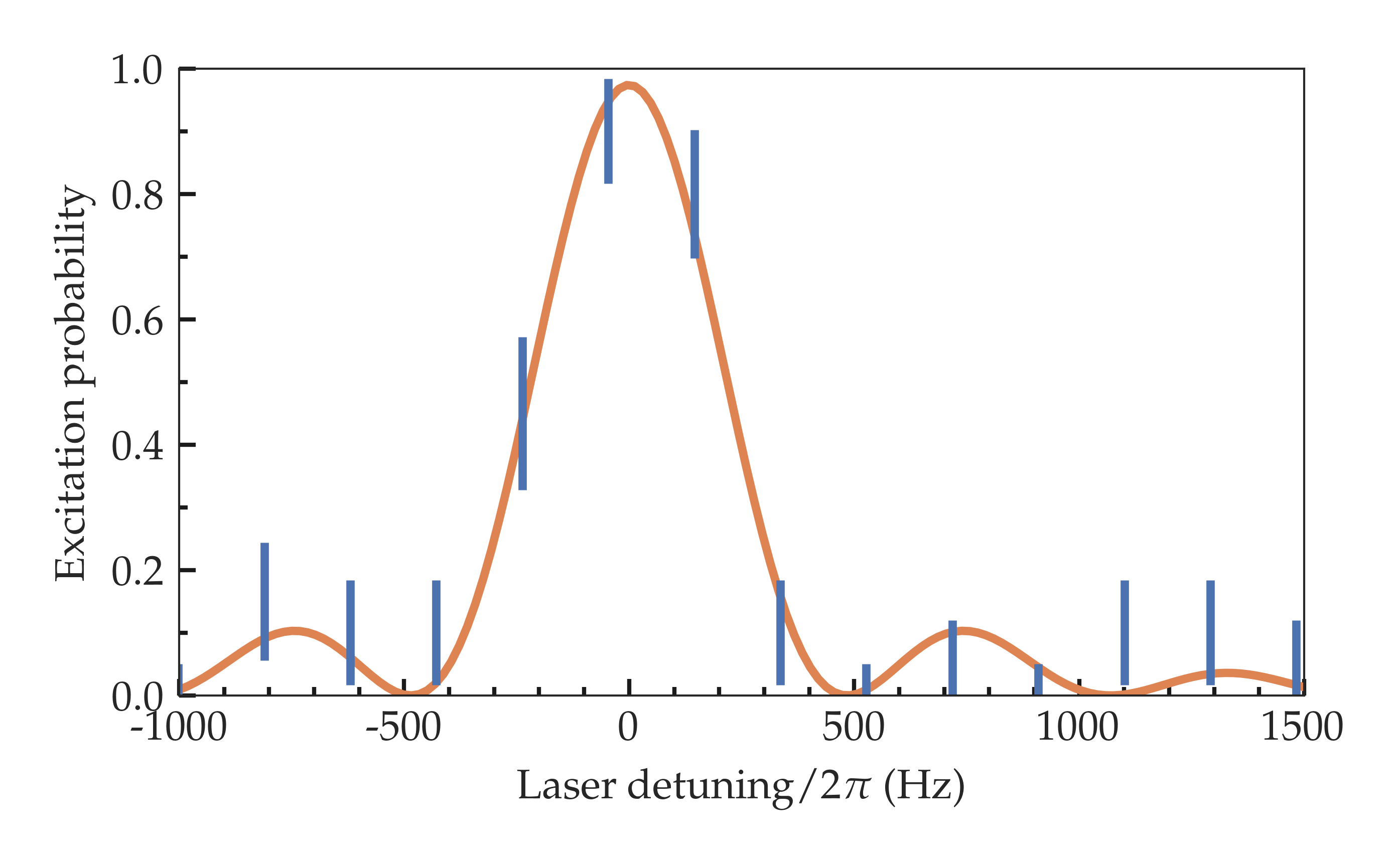
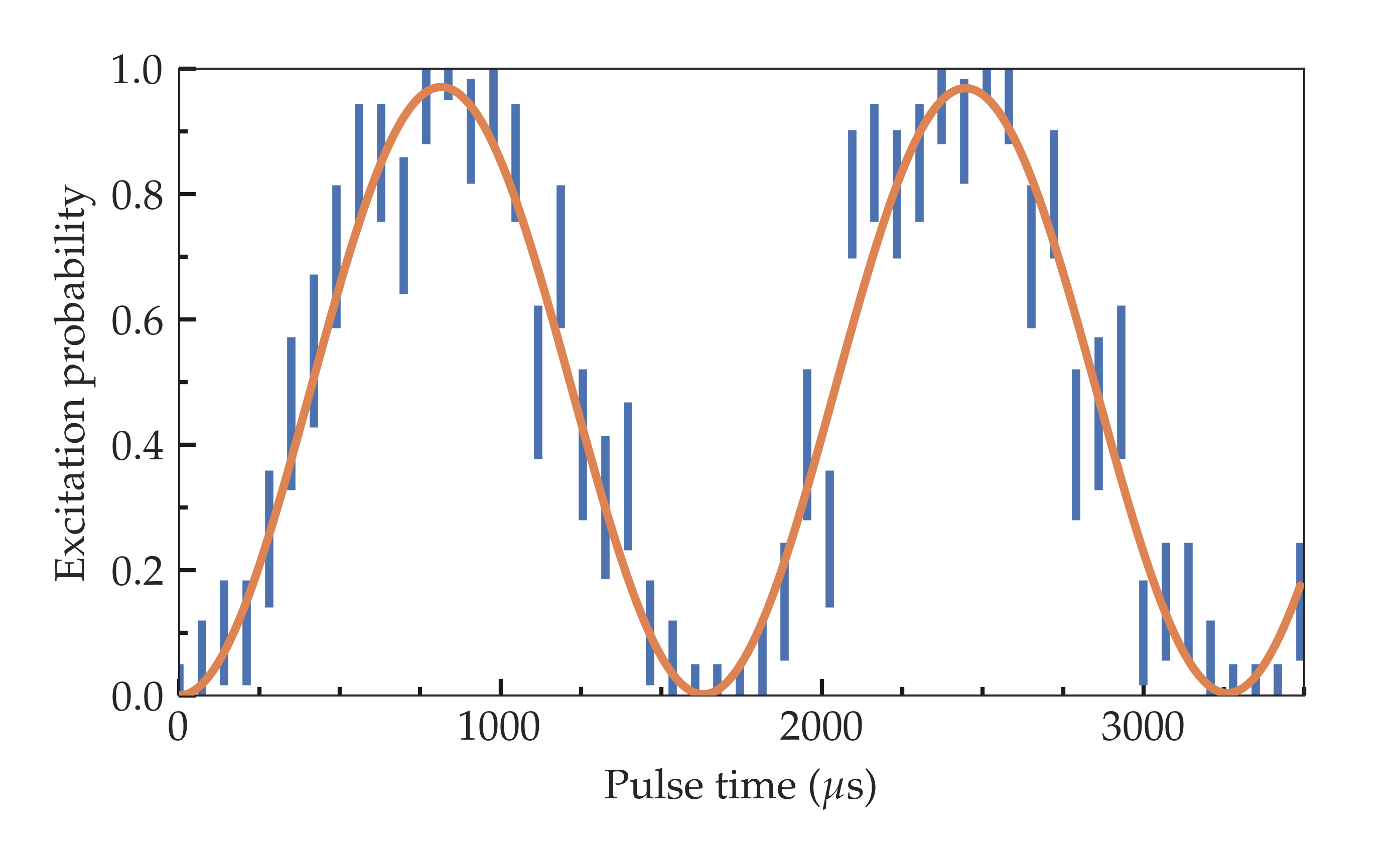
Figure 6: Example measurements for the determination of one transition frequency and coupling strength data point pair. The excitation data (blue) was fitted (orange) to extract: (a) The center frequency of one CDD transition using a laser detuning scan. (b) The coupling strength of the same transition using pulse time spectroscopy. For better frequency resolution, the frequency scan was taken with less optical power, thus higher resolution.

A sinosoidal fit of the Rabi flopping signal is used to extract the optical coupling strength. This procedure was repeated for all transitions. The resolution of the individual scans was chosen as a compromise between sufficient low uncertainty and data acquisition speed. The latter is important in order to minimize the uncertainties of drifting static B-field and coupling strength over the course of a complete series of measurements. The acquired data is summarized in Tab. 2.

m	M	$\mkern-1.7mum\mkern-1.7mu$	$\mkern-1.7muM\mkern-1.7mu$	$\Delta_{L,\text{calc}}$ (MHz)	$\Delta_{L,\text{exp}}$ (MHz)	$\frac{\Omega^{m,M}_{\bar{m},\bar{M}}}{\Omega_{m,M}}$ (calc)	$\Omega^{m,M}_{\bar{m},\bar{M}}$ (kHz)
-0.5	-1.5	0.5	-2.5	-4.18903	-4.18906	0.27493	0.46923
-0.5	-1.5	-0.5	-2.5	-4.14213	-4.14214	0.28640	0.45828
-0.5	-1.5	0.5	-1.5	-4.11965	-4.11970	0.36708	0.62568
-0.5	-1.5	-0.5	-1.5	-4.07275	-4.07281	0.38239	0.62326
-0.5	-1.5	0.5	-0.5	-4.05027	-4.05028	0.17087	0.29412
-0.5	-1.5	-0.5	-0.5	-4.00337	-4.00337	0.17799	0.29951
-0.5	-1.5	0.5	0.5	-3.98089	-3.98091	0.17538	0.27588
-0.5	-1.5	-0.5	0.5	-3.93399	-3.93401	0.18270	0.26195
-0.5	-1.5	0.5	1.5	-3.91151	-3.91156	0.36743	0.61065
-0.5	-1.5	-0.5	1.5	-3.86461	-3.86458	0.38276	0.61313
-0.5	-1.5	0.5	2.5	-3.84213	-3.84216	0.27255	0.45904
-0.5	-1.5	-0.5	2.5	-3.79523	-3.79526	0.28392	0.45519
-0.5	-2.5	0.5	-2.5	-10.18386	-10.18395	0.12331	0.23861
-0.5	-2.5	-0.5	-2.5	-10.13697	-10.13702	0.12845	0.22617
-0.5	-2.5	0.5	-1.5	-10.11448	-10.11448	0.27493	0.52114
-0.5	-2.5	-0.5	-1.5	-10.06759	-10.06771	0.28640	0.52519
-0.5	-2.5	0.5	-0.5	-10.04510	-10.04488	0.38769	0.81061
-0.5	-2.5	-0.5	-0.5	-9.99821	-9.99805	0.40385	0.77476
-0.5	-2.5	0.5	0.5	-9.97572	-9.97573	0.38657	0.78431
-0.5	-2.5	-0.5	0.5	-9.92883	-9.92877	0.40269	0.77869
-0.5	-2.5	0.5	1.5	-9.90634	-9.90644	0.27255	0.54841
-0.5	-2.5	-0.5	1.5	-9.85945	-9.85939	0.28392	0.55880
-0.5	-2.5	0.5	2.5	-9.83696	-9.83703	0.12154	0.24665
-0.5	-2.5	-0.5	2.5	-9.79007	-9.79012	0.12661	0.24661

Table 2: Data used for Fig. 5.

References

- Hahn (1950) E. L. Hahn, Spin echoes, Physical Review 80, 580 (1950).
- Souza et al. (2012) A. M. Souza, G. A. Álvarez, and D. Suter, Robust dynamical decoupling, Philosophical Transactions of the Royal Society A: Mathematical, Physical and Engineering Sciences 370, 4748 (2012).
- Viola and Lloyd (1998) L. Viola and S. Lloyd, Dynamical suppression of decoherence in two-state quantum systems, Physical Review A: Atomic, Molecular, and Optical Physics 58 (1998), 10.1103/PhysRevA.58.2733.
- Viola et al. (1999) L. Viola, E. Knill, and S. Lloyd, Dynamical decoupling of open quantum systems, Physical Review Letters 82 (1999), 10.1103/PhysRevLett.82.2417.
- Zanardi (1999) P. Zanardi, Symmetrizing evolutions, Physics Letters A 258 (1999), 10.1016/S0375-9601(99)00365-5.
- Byrd and Lidar (2002) M. S. Byrd and D. A. Lidar, Quantum Information Processing 1 (2002), 10.1023/a:1019697017584.
- Facchi et al. (2005) P. Facchi, S. Tasaki, S. Pascazio, H. Nakazato, A. Tokuse, and D. A. Lidar, Control of decoherence: Analysis and comparison of three different strategies, Physical Review A 71 (2005), 10.1103/physreva.71.022302.
- Khodjasteh and Lidar (2008) K. Khodjasteh and D. A. Lidar, Rigorous bounds on the performance of a hybrid dynamical-decoupling quantum-computing scheme, Physical Review A 78 (2008), 10.1103/physreva.78.012355.
- Khodjasteh and Viola (2009a) K. Khodjasteh and L. Viola, Dynamically error-corrected gates for universal quantum computation, Physical Review Letters 102 (2009a), 10.1103/physrevlett.102.080501.
- Khodjasteh and Viola (2009b) K. Khodjasteh and L. Viola, Dynamical quantum error correction of unitary operations with bounded controls, Physical Review A 80 (2009b), 10.1103/physreva.80.032314.
- Khodjasteh et al. (2010) K. Khodjasteh, D. A. Lidar, and L. Viola, Arbitrarily accurate dynamical control in open quantum systems, Physical Review Letters 104 (2010), 10.1103/physrevlett.104.090501.
- D.A (2012) L. D.A, Review of decoherence free subspaces, noiseless subsystems, and dynamical decoupling, Adv. Chem. Phys. 154, 295 (2012), arXiv:1208.5791.
- Aharon et al. (2019) N. Aharon, N. Spethmann, I. D. Leroux, P. O. Schmidt, and A. Retzker, Robust optical clock transitions in trapped ions using dynamical decoupling, New Journal of Physics 21 (2019), 10.1088/1367-2630/ab3871.
- Green et al. (2013) T. J. Green, J. Sastrawan, H. Uys, and M. J. Biercuk, Arbitrary quantum control of qubits in the presence of universal noise, New Journal of Physics 15, 095004 (2013).
- West et al. (2010) J. R. West, D. A. Lidar, B. H. Fong, and M. F. Gyure, High Fidelity Quantum Gates via Dynamical Decoupling, Physical Review Letters 105, 230503 (2010).
- Uhrig (2007) G. S. Uhrig, Keeping a quantum bit alive by optimized -pulse sequences, Physical Review Letters 98, 100504 (2007).
- Haeberlen and Waugh (1968) U. Haeberlen and J. S. Waugh, Coherent Averaging Effects in Magnetic Resonance, Physical Review 175, 453 (1968).
- Biercuk et al. (2009) M. J. Biercuk, H. Uys, A. P. VanDevender, N. Shiga, W. M. Itano, and J. J. Bollinger, Optimized dynamical decoupling in a model quantum memory, Nature 458 (2009), 10.1038/nature07951.
- Du et al. (2009) J. Du, X. Rong, N. Zhao, Y. Wang, J. Yang, and R. B. Liu, Preserving electron spin coherence in solids by optimal dynamical decoupling, Nature 461 (2009), 10.1038/nature08470.
- Damodarakurup et al. (2009) S. Damodarakurup, M. Lucamarini, G. D. Giuseppe, D. Vitali, and P. Tombesi, Experimental inhibition of decoherence on flying qubits via “Bang-Bang” control, Physical Review Letters 103 (2009), 10.1103/physrevlett.103.040502.
- de Lange et al. (2010) G. de Lange, Z. H. Wang, D. Ristè, V. V. Dobrovitski, and R. Hanson, Universal Dynamical Decoupling of a Single Solid-State Spin from a Spin Bath, Science (New York, N.Y.) 330, 60 (2010).
- Souza et al. (2011) A. M. Souza, G. A. Álvarez, and D. Suter, Robust dynamical decoupling for quantum computing and quantum memory, Physical Review Letters 106 (2011), 10.1103/physrevlett.106.240501.
- Naydenov et al. (2011) B. Naydenov, F. Dolde, L. T. Hall, C. Shin, H. Fedder, L. C. L. Hollenberg, F. Jelezko, and J. Wrachtrup, Dynamical decoupling of a single-electron spin at room temperature, Physical Review B 83 (2011), 10.1103/physrevb.83.081201.
- van der Sar et al. (2012) T. van der Sar, Z. H. Wang, M. S. Blok, H. Bernien, T. H. Taminiau, D. M. Toyli, D. A. Lidar, D. D. Awschalom, R. Hanson, and V. V. Dobrovitski, Decoherence-protected quantum gates for a hybrid solid-state spin register, Nature 484 (2012), 10.1038/nature10900.
- Shaniv et al. (2019) R. Shaniv, N. Akerman, T. Manovitz, Y. Shapira, and R. Ozeri, Quadrupole Shift Cancellation Using Dynamic Decoupling, Physical Review Letters 122, 223204 (2019).
- Wang et al. (2017) Y. Wang, M. Um, J. Zhang, S. An, M. Lyu, J.-N. Zhang, L.-M. Duan, D. Yum, and K. Kim, Single-qubit quantum memory exceeding ten-minute coherence time, Nature Photonics 11, 646 (2017).
- Qiu et al. (2021) J. Qiu, Y. Zhou, C.-K. Hu, J. Yuan, L. Zhang, J. Chu, W. Huang, W. Liu, K. Luo, Z. Ni, X. Pan, Z. Yang, Y. Zhang, Y. Chen, X.-H. Deng, L. Hu, J. Li, J. Niu, Y. Xu, T. Yan, Y. Zhong, S. Liu, F. Yan, and D. Yu, Suppressing Coherent Two-Qubit Errors via Dynamical Decoupling, Physical Review Applied 16, 054047 (2021).
- Zhou et al. (2020) H. Zhou, J. Choi, S. Choi, R. Landig, A. M. Douglas, J. Isoya, F. Jelezko, S. Onoda, H. Sumiya, P. Cappellaro, H. S. Knowles, H. Park, and M. D. Lukin, Quantum Metrology with Strongly Interacting Spin Systems, Physical Review X 10, 031003 (2020).
- Manovitz et al. (2017) T. Manovitz, A. Rotem, R. Shaniv, I. Cohen, Y. Shapira, N. Akerman, A. Retzker, and R. Ozeri, Fast dynamical decoupling of the Mølmer-Sørensen entangling gate, Physical Review Letters 119, 220505 (2017).
- Shaniv et al. (2016) R. Shaniv, N. Akerman, and R. Ozeri, Atomic Quadrupole Moment Measurement Using Dynamic Decoupling, Physical Review Letters 116, 140801 (2016).
- Piltz et al. (2013) C. Piltz, B. Scharfenberger, A. Khromova, A. F. Varón, and C. Wunderlich, Protecting Conditional Quantum Gates by Robust Dynamical Decoupling, Physical Review Letters 110, 200501 (2013).
- Kuwahara et al. (2016) T. Kuwahara, T. Mori, and K. Saito, Floquet–Magnus theory and generic transient dynamics in periodically driven many-body quantum systems, Annals of Physics 367, 96 (2016).
- Fonseca-Romero et al. (2005) K. M. Fonseca-Romero, S. Kohler, and P. Hänggi, Coherence stabilization of a two-qubit gate by ac fields, Physical Review Letters 95 (2005), 10.1103/PhysRevLett.95.140502.
- Chen (2006) P. Chen, Geometric continuous dynamical decoupling with bounded controls, Physical Review A: Atomic, Molecular, and Optical Physics 73 (2006), 10.1103/PhysRevA.73.022343.
- Yalçınkaya et al. (2019) İ. Yalçınkaya, B. Çakmak, G. Karpat, and F. F. Fanchini, Continuous dynamical decoupling and decoherence-free subspaces for qubits with tunable interaction, Quantum Information Processing 18 (2019), 10.1007/s11128-019-2271-0.
- Clausen et al. (2010) J. Clausen, G. Bensky, and G. Kurizki, Bath-optimized minimal-energy protection of quantum operations from decoherence, Physical Review Letters 104 (2010), 10.1103/PhysRevLett.104.040401.
- Xu et al. (2012) X. Xu, Z. Wang, C. Duan, P. Huang, P. Wang, Y. Wang, N. Xu, X. Kong, F. Shi, X. Rong, and J. Du, Coherence-Protected Quantum Gate by Continuous Dynamical Decoupling in Diamond, Physical Review Letters 109, 070502 (2012).
- Fanchini et al. (2007) F. F. Fanchini, J. E. M. Hornos, and R. d. J. Napolitano, Continuously decoupling single-qubit operations from a perturbing thermal bath of scalar bosons, Physical Review A: Atomic, Molecular, and Optical Physics 75 (2007), 10.1103/PhysRevA.75.022329.
- Fanchini and Napolitano (2007) F. F. Fanchini and R. d. J. Napolitano, Continuous dynamical protection of two-qubit entanglement from uncorrelated dephasing, bit flipping, and dissipation, Physical Review A: Atomic, Molecular, and Optical Physics 76 (2007), 10.1103/PhysRevA.76.062306.
- Fanchini et al. (2015) F. F. Fanchini, R. d. J. Napolitano, B. ÇÇakmak, and A. O. Caldeira, Protecting the SWAP operation from general and residual errors by continuous dynamical decoupling, Physical Review A: Atomic, Molecular, and Optical Physics 91 (2015), 10.1103/PhysRevA.91.042325.
- Rabl et al. (2009) P. Rabl, P. Cappellaro, M. V. G. Dutt, L. Jiang, J. R. Maze, and M. D. Lukin, Strong magnetic coupling between an electronic spin qubit and a mechanical resonator, Physical Review B 79 (2009), 10.1103/PhysRevB.79.041302.
- Chaudhry and Gong (2012) A. Z. Chaudhry and J. Gong, Decoherence control: Universal protection of two-qubit states and two-qubit gates using continuous driving fields, Physical Review A: Atomic, Molecular, and Optical Physics 85 (2012), 10.1103/PhysRevA.85.012315.
- Cai et al. (2012) J.-M. Cai, B. Naydenov, R. Pfeiffer, L. P. McGuinness, K. D. Jahnke, F. Jelezko, M. B. Plenio, and A. Retzker, Robust dynamical decoupling with concatenated continuous driving, New Journal of Physics 14 (2012), 10.1088/1367-2630/14/11/113023.
- Laraoui and Meriles (2011) A. Laraoui and C. A. Meriles, Rotating frame spin dynamics of a nitrogen-vacancy center in a diamond nanocrystal, Physical Review B 84 (2011), 10.1103/PhysRevB.84.161403.
- Bermudez et al. (2011) A. Bermudez, F. Jelezko, M. B. Plenio, and A. Retzker, Electron-mediated nuclear-spin interactions between distant nitrogen-vacancy centers, Physical Review Letters 107 (2011), 10.1103/PhysRevLett.107.150503.
- Bermudez et al. (2012) A. Bermudez, P. O. Schmidt, M. B. Plenio, and A. Retzker, Robust trapped-ion quantum logic gates by continuous dynamical decoupling, Physical Review A: Atomic, Molecular, and Optical Physics 85 (2012), 10.1103/PhysRevA.85.040302.
- Timoney et al. (2011) N. Timoney, I. Baumgart, M. Johanning, A. F. Varón, M. B. Plenio, A. Retzker, and C. Wunderlich, Quantum gates and memory using microwave-dressed states, Nature 476 (2011), 10.1038/nature10319.
- Doherty et al. (2013) M. W. Doherty, N. B. Manson, P. Delaney, F. Jelezko, J. Wrachtrup, and L. C. Hollenberg, The nitrogen-vacancy colour centre in diamond, Physics Reports 528 (2013), 10.1016/j.physrep.2013.02.001.
- Albrecht et al. (2014) A. Albrecht, G. Koplovitz, A. Retzker, F. Jelezko, S. Yochelis, D. Porath, Y. Nevo, O. Shoseyov, Y. Paltiel, and M. B Plenio, Self-assembling hybrid diamond–biological quantum devices, New Journal of Physics 16 (2014), 10.1088/1367-2630/16/9/093002.
- Golter et al. (2014) D. A. Golter, T. K. Baldwin, and H. Wang, Protecting a solid-state spin from decoherence using dressed spin states, Physical Review Letters 113 (2014), 10.1103/PhysRevLett.113.237601.
- Finkelstein et al. (2021) R. Finkelstein, O. Lahad, I. Cohen, O. Davidson, S. Kiriati, E. Poem, and O. Firstenberg, Continuous Protection of a Collective State from Inhomogeneous Dephasing, Physical Review X 11, 011008 (2021).
- Trypogeorgos et al. (2018) D. Trypogeorgos, A. Valdés-Curiel, N. Lundblad, and I. B. Spielman, Synthetic clock transitions via continuous dynamical decoupling, Physical Review A: Atomic, Molecular, and Optical Physics 97, 013407 (2018).
- Anderson et al. (2018) R. P. Anderson, M. J. Kewming, and L. D. Turner, Continuously observing a dynamically decoupled spin-1 quantum gas, Physical Review A: Atomic, Molecular, and Optical Physics 97, 013408 (2018).
- Laucht et al. (2017) A. Laucht, R. Kalra, S. Simmons, J. P. Dehollain, J. T. Muhonen, F. A. Mohiyaddin, S. Freer, F. E. Hudson, K. M. Itoh, D. N. Jamieson, J. C. McCallum, A. S. Dzurak, and A. Morello, A dressed spin qubit in silicon, Nature Nanotechnology 12, 61 (2017).
- Sárkány et al. (2014) L. Sárkány, P. Weiss, H. Hattermann, and J. Fortágh, Controlling the magnetic-field sensitivity of atomic-clock states by microwave dressing, Physical Review A: Atomic, Molecular, and Optical Physics 90, 053416 (2014).
- Webster et al. (2013) S. C. Webster, S. Weidt, K. Lake, J. J. McLoughlin, and W. K. Hensinger, Simple Manipulation of a Microwave Dressed-State Ion Qubit, Physical Review Letters 111, 140501 (2013).
- Tan et al. (2013) T. R. Tan, J. P. Gaebler, R. Bowler, Y. Lin, J. D. Jost, D. Leibfried, and D. J. Wineland, Demonstration of a Dressed-State Phase Gate for Trapped Ions, Physical Review Letters 110, 263002 (2013).
- Aharon et al. (2013) N. Aharon, M. Drewsen, and A. Retzker, General Scheme for the Construction of a Protected Qubit Subspace, Physical Review Letters 111, 230507 (2013).
- Zanon-Willette et al. (2012) T. Zanon-Willette, E. de Clercq, and E. Arimondo, Magic Radio-Frequency Dressing of Nuclear Spins in High-Accuracy Optical Clocks, Physical Review Letters 109, 223003 (2012).
- Kessler et al. (2014) E. M. Kessler, P. Kómár, M. Bishof, L. Jiang, A. S. Sørensen, J. Ye, and M. D. Lukin, Heisenberg-Limited Atom Clocks Based on Entangled Qubits, Physical Review Letters 112, 190403 (2014).
- Peik et al. (2005) E. Peik, T. Schneider, and C. Tamm, Laser frequency stabilization to a single ion, Journal of Physics B: Atomic, Molecular and Optical Physics 39 (2005), 10.1088/0953-4075/39/1/012.
- Leroux et al. (2017) I. D. Leroux, N. Scharnhorst, S. Hannig, J. Kramer, L. Pelzer, M. Stepanova, and P. O. Schmidt, On-line estimation of local oscillator noise and optimisation of servo parameters in atomic clocks, Metrologia 54 (2017), 10.1088/1681-7575/aa66e9.
- Keller et al. (2019) J. Keller, D. Kalincev, T. Burgermeister, A. P. Kulosa, A. Didier, T. Nordmann, J. Kiethe, and T. Mehlstäubler, Probing time dilation in coulomb crystals in a high-precision ion trap, Physical Review Applied 11 (2019), 10.1103/PhysRevApplied.11.011002.
- Arnold et al. (2015) K. Arnold, E. Hajiyev, E. Paez, C. H. Lee, M. D. Barrett, and J. Bollinger, Prospects for atomic clocks based on large ion crystals, Physical Review A: Atomic, Molecular, and Optical Physics 92, 032108 (2015).
- Herschbach et al. (2012) N. Herschbach, K. Pyka, J. Keller, and T. E. Mehlstäubler, Linear Paul trap design for an optical clock with Coulomb crystals, Applied Physics B 107 (2012), 10.1007/s00340-011-4790-y.
- Champenois et al. (2010) C. Champenois, M. Marciante, J. Pedregosa-Gutierrez, M. Houssin, M. Knoop, and M. Kajita, Ion ring in a linear multipole trap for optical frequency metrology, Physical Review A: Atomic, Molecular, and Optical Physics 81 (2010), 10.1103/PhysRevA.81.043410.
- Itano (2000) W. Itano, External-field shifts of the 199Hg+ optical frequency standard, Journal of Research of the National Institute of Standards and Technology 105 (2000), 10.6028/jres.105.065.
- Berkeland et al. (1998) D. J. Berkeland, J. D. Miller, J. C. Bergquist, W. M. Itano, and D. J. Wineland, Minimization of ion micromotion in a Paul trap, Journal of Applied Physics 83 (1998), 10.1063/1.367318.
- Schneider et al. (2005) T. Schneider, E. Peik, and C. Tamm, Sub-hertz optical frequency comparisons between two trapped 171Yb+ ions, Physical Review Letters 94 (2005), 10.1103/physrevlett.94.230801.
- Dubé et al. (2005) P. Dubé, A. Madej, J. Bernard, L. Marmet, J.-S. Boulanger, and S. Cundy, Electric Quadrupole Shift Cancellation in Single-Ion Optical Frequency Standards, Physical Review Letters 95, 033001 (2005).
- Tan et al. (2019) T. R. Tan, R. Kaewuam, K. J. Arnold, S. R. Chanu, Z. Zhang, M. S. Safronova, and M. D. Barrett, Suppressing Inhomogeneous Broadening in a Lutetium Multi-ion Optical Clock, Physical Review Letters 123, 063201 (2019).
- Lange et al. (2020) R. Lange, N. Huntemann, C. Sanner, H. Shao, B. Lipphardt, C. Tamm, and E. Peik, Coherent Suppression of Tensor Frequency Shifts through Magnetic Field Rotation, Physical Review Letters 125 (2020), 10.1103/PhysRevLett.125.143201.
- Andrew et al. (1958) E. R. Andrew, A. Bradbury, and R. G. Eades, Nuclear Magnetic Resonance Spectra from a Crystal rotated at High Speed, Nature 182 (1958), 10.1038/1821659a0.
- Kaewuam et al. (2020) R. Kaewuam, T. R. Tan, K. J. Arnold, S. R. Chanu, Z. Zhang, and M. D. Barrett, Hyperfine Averaging by Dynamic Decoupling in a Multi-Ion Lutetium Clock, Physical Review Letters 124, 083202 (2020).
- Martínez (2022) V. Martínez, Relativistic Corrections and Dynamic Decoupling in Trapped Ion Optical Atomic Clocks, Ph.D. thesis, Leibniz University Hannover (2022).
- James (1998) D. James, Quantum dynamics of cold trapped ions with application to quantum computation, Applied Physics B: Lasers and Optics 66 (1998), 10.1007/s003400050373.
- Dalibard and Cohen-Tannoudji (1985) J. Dalibard and C. Cohen-Tannoudji, Dressed-atom approach to atomic motion in laser light: The dipole force revisited, JOSA B 2, 1707 (1985).
- Tommaseo et al. (2003) G. Tommaseo, T. Pfeil, G. Revalde, G. Werth, P. Indelicato, and J. P. Desclaux, The gJ-factor in the ground state of Ca+, The European Physical Journal D - Atomic, Molecular, Optical and Plasma Physics 25 (2003), 10.1140/epjd/e2003-00096-6.
- Chwalla et al. (2009) M. Chwalla, J. Benhelm, K. Kim, G. Kirchmair, T. Monz, M. Riebe, P. Schindler, A. Villar, W. Hänsel, C. Roos, R. Blatt, M. Abgrall, G. Santarelli, G. Rovera, and P. Laurent, Absolute frequency measurement of the 40Ca+ clock transition, Physical Review Letters 102, 023002 (2009).
- Monz et al. (2011) T. Monz, P. Schindler, J. T. Barreiro, M. Chwalla, D. Nigg, W. A. Coish, M. Harlander, W. Hänsel, M. Hennrich, and R. Blatt, 14-Qubit Entanglement: Creation and Coherence, Physical Review Letters 106, 130506 (2011).
- Kaushal et al. (2020) V. Kaushal, B. Lekitsch, A. Stahl, J. Hilder, D. Pijn, C. Schmiegelow, A. Bermudez, M. Müller, F. Schmidt-Kaler, and U. Poschinger, Shuttling-based trapped-ion quantum information processing, AVS Quantum Science 2, 014101 (2020).
- Ringbauer et al. (2022) M. Ringbauer, M. Meth, L. Postler, R. Stricker, R. Blatt, P. Schindler, and T. Monz, A universal qudit quantum processor with trapped ions, Nature Physics 18, 1053 (2022).
- Pogorelov et al. (2021) I. Pogorelov, T. Feldker, C. D. Marciniak, L. Postler, G. Jacob, O. Krieglsteiner, V. Podlesnic, M. Meth, V. Negnevitsky, M. Stadler, B. Höfer, C. Wächter, K. Lakhmanskiy, R. Blatt, P. Schindler, and T. Monz, Compact Ion-Trap Quantum Computing Demonstrator, PRX Quantum 2, 020343 (2021).
- Hilder et al. (2022) J. Hilder, D. Pijn, O. Onishchenko, A. Stahl, M. Orth, B. Lekitsch, A. Rodriguez-Blanco, M. Müller, F. Schmidt-Kaler, and U. G. Poschinger, Fault-Tolerant Parity Readout on a Shuttling-Based Trapped-Ion Quantum Computer, Physical Review X 12, 011032 (2022).
- Joshi et al. (2022) M. K. Joshi, F. Kranzl, A. Schuckert, I. Lovas, C. Maier, R. Blatt, M. Knap, and C. F. Roos, Observing emergent hydrodynamics in a long-range quantum magnet, Science (New York, N.Y.) 376, 720 (2022).
- Kokail et al. (2019) C. Kokail, C. Maier, R. van Bijnen, T. Brydges, M. K. Joshi, P. Jurcevic, C. A. Muschik, P. Silvi, R. Blatt, C. F. Roos, and P. Zoller, Self-verifying variational quantum simulation of lattice models, Nature 569, 355 (2019).
- Hempel et al. (2018) C. Hempel, C. Maier, J. Romero, J. McClean, T. Monz, H. Shen, P. Jurcevic, B. P. Lanyon, P. Love, R. Babbush, A. Aspuru-Guzik, R. Blatt, and C. F. Roos, Quantum Chemistry Calculations on a Trapped-Ion Quantum Simulator, Physical Review X 8, 031022 (2018).
- Matsubara et al. (2012) K. Matsubara, H. Hachisu, Y. Li, S. Nagano, C. Locke, A. Nogami, M. Kajita, K. Hayasaka, T. Ido, and M. Hosokawa, Direct comparison of a Ca+ single-ion clock against a Sr lattice clock to verify the absolute frequency measurement, Optics Express 20, 22034 (2012).
- Huang et al. (2019) Y. Huang, H. Guan, M. Zeng, L. Tang, and K. Gao, 40Ca+ ion optical clock with micromotion-induced shifts below , Physical Review A 99, 011401 (2019).
- Huang et al. (2021) Y. Huang, B. Zhang, M. Zeng, Y. Hao, H. Zhang, H. Guan, Z. Chen, M. Wang, and K. Gao, A liquid nitrogen-cooled Ca+ optical clock with systematic uncertainty of , ArXiv210308913 Phys. (2021), arXiv:2103.08913 [physics] .
- Cao et al. (2017) J. Cao, P. Zhang, J. Shang, K. Cui, J. Yuan, S. Chao, S. Wang, H. Shu, and X. Huang, A compact, transportable single-ion optical clock with 7.8×10⁻¹⁷ systematic uncertainty, Applied Physics B: Photophysics and Laser Chemistry 123, 112 (2017).
- Li et al. (2022) W. Li, S. Wolf, L. Klein, D. Budker, C. E. Düllmann, and F. Schmidt-Kaler, Robust polarization gradient cooling of trapped ions, New Journal of Physics 24, 043028 (2022).
- Morigi et al. (2000) G. Morigi, J. Eschner, and C. H. Keitel, Ground State Laser Cooling Using Electromagnetically Induced Transparency, Physical Review Letters 85 (2000), 10.1103/PhysRevLett.85.4458.
- Scharnhorst et al. (2018) N. Scharnhorst, J. Cerrillo, J. Kramer, I. D. Leroux, J. B. Wübbena, A. Retzker, and P. O. Schmidt, Experimental and theoretical investigation of a multimode cooling scheme using multiple electromagnetically-induced-transparency resonances, Physical Review A 98 (2018), 10.1103/PhysRevA.98.023424.
- Lechner et al. (2016) R. Lechner, C. Maier, C. Hempel, P. Jurcevic, B. P. Lanyon, T. Monz, M. Brownnutt, R. Blatt, and C. F. Roos, Electromagnetically-induced-transparency ground-state cooling of long ion strings, Physical Review A: Atomic, Molecular, and Optical Physics 93 (2016), 10.1103/PhysRevA.93.053401.
- Hannig et al. (2019) S. Hannig, L. Pelzer, N. Scharnhorst, J. Kramer, M. Stepanova, Z. T. Xu, N. Spethmann, I. D. Leroux, T. E. Mehlstäubler, and P. O. Schmidt, Towards a transportable aluminium ion quantum logic optical clock, Review of Scientific Instruments 90 (2019), 10.1063/1.5090583.
- Note (1) High Finesse U10.
- Note (2) TA pro, Toptica.
- Drever et al. (1983) R. W. P. Drever, J. L. Hall, F. V. Kowalski, J. Hough, G. M. Ford, A. J. Munley, and H. Ward, Laser phase and frequency stabilization using an optical resonator, Applied Physics B 31 (1983), 10.1007/BF00702605.
- Scharnhorst et al. (2015) N. Scharnhorst, J. B. Wübbena, S. Hannig, K. Jakobsen, J. Kramer, I. D. Leroux, and P. O. Schmidt, High-bandwidth transfer of phase stability through a fiber frequency comb, Optics Express 23 (2015), 10.1364/OE.23.019771.
- Matei et al. (2017) D. G. Matei, T. Legero, S. Häfner, C. Grebing, R. Weyrich, W. Zhang, L. Sonderhouse, J. M. Robinson, J. Ye, F. Riehle, and U. Sterr, 1.5m Lasers with Sub-10 mHz Linewidth, Physical Review Letters 118 (2017), 10.1103/PhysRevLett.118.263202.
- Benkler et al. (2019) E. Benkler, B. Lipphardt, T. Puppe, R. Wilk, F. Rohde, and U. Sterr, End-to-end topology for fiber comb based optical frequency transfer at the 10-21 level, Optics Express 27 (2019), 10.1364/OE.27.036886.
- Schindler (2008) P. Schindler, Frequency Synthesis and Pulse Shaping for Quantum Information Processing with Trapped Ions, Diploma Thesis, University of Innsbruck, Innsbruck, Austria (2008).
- Pham (2005) P. T. T. Pham, A General-Purpose Pulse Sequencer for Quantum Computing, Ph.D. thesis, Massachusetts Institute of Technology, Cambridge, Massachusetts, USA (2005).
- Note (3) Keysight 33622A.
- Roos et al. (2000) C. F. Roos, D. Leibfried, A. Mundt, F. Schmidt-Kaler, J. Eschner, and R. Blatt, Experimental demonstration of ground state laser cooling with electromagnetically induced transparency, Physical Review Letters 85, 5547 (2000).
- Wunderlich et al. (2007) C. Wunderlich, T. Hannemann, T. Körber, H. Häffner, C. Roos, W. Hänsel, R. Blatt, and F. Schmidt-Kaler, Robust state preparation of a single trapped ion by adiabatic passage, Journal of Modern Optics 54 (2007), 10.1080/09500340600741082.
- Leibfried et al. (2004) D. Leibfried, M. D. Barrett, T. Schaetz, J. Britton, J. Chiaverini, W. M. Itano, J. D. Jost, C. Langer, and D. J. Wineland, Toward Heisenberg-Limited Spectroscopy with Multiparticle Entangled States, Science (New York, N.Y.) 304, 1476 (2004).
- Nichol et al. (2022) B. C. Nichol, R. Srinivas, D. P. Nadlinger, P. Drmota, D. Main, G. Araneda, C. J. Ballance, and D. M. Lucas, An elementary quantum network of entangled optical atomic clocks, Nature , 1 (2022).
- Schulte et al. (2020) M. Schulte, C. Lisdat, P. O. Schmidt, U. Sterr, and K. Hammerer, Prospects and challenges for squeezing-enhanced optical atomic clocks, Nature Communications 11, 5955 (2020).
- Häffner et al. (2008) H. Häffner, C. Roos, and R. Blatt, Quantum computing with trapped ions, Physics Reports 469, 155 (2008).
- Magnus (1954) W. Magnus, On the exponential solution of differential equations for a linear operator, Communications on Pure and Applied Mathematics 7 (1954), 10.1002/cpa.3160070404.
- Galindo and Pascual (2012) A. Galindo and P. Pascual, Quantum Mechanics I (Springer Berlin, Heidelberg, 2012).