XTrace: Making the most of every sample
in stochastic trace estimation

Abstract

The implicit trace estimation problem asks for an approximation of the trace of a square matrix, accessed via matrix–vector products (matvecs). This paper designs new randomized algorithms, XTrace and XNysTrace, for the trace estimation problem by exploiting both variance reduction and the exchangeability principle. For a fixed budget of matvecs, numerical experiments show that the new methods can achieve errors that are orders of magnitude smaller than existing algorithms, such as the Girard–Hutchinson estimator or the Hutch++ estimator. A theoretical analysis confirms the benefits by offering a precise description of the performance of these algorithms as a function of the spectrum of the input matrix. The paper also develops an exchangeable estimator, XDiag, for approximating the diagonal of a square matrix using matvecs.

65C05, 65F30, 68W20

1 Introduction

Over the past three decades, researchers have developed randomized algorithms for linear algebra problems such as trace estimation [14, 19, 26], low-rank approximation [15], and over-determined least squares [3, 30]. Many of these algorithms collect information by judicious random sampling of the problem data. As a consequence, we can design better algorithms using techniques from the theory of statistical estimation, such as variance reduction and the exchangeability principle. This paper explores how the exchangeability principle leads to faster randomized algorithms for trace estimation.

Suppose that we wish to compute a quantity $Q(\boldsymbol{A})$ associated with a matrix $\boldsymbol{A}$. A typical randomized algorithm might proceed as follows.

1. Collect information about the matrix $\boldsymbol{A}$ by computing matrix–vector products $\boldsymbol{A}\boldsymbol{\omega}_{1},\ldots,\boldsymbol{A}\boldsymbol{\omega}_{k}$ with random test vectors $\boldsymbol{\omega}_{1},\ldots,\boldsymbol{\omega}_{k}$.

2. Form an estimate of $Q(\boldsymbol{A})$ from the samples $\boldsymbol{A}\boldsymbol{\omega}_{1},\ldots,\boldsymbol{A}\boldsymbol{\omega}_{k}$.

The question arises: Given the data $\boldsymbol{A}\boldsymbol{\omega}_{1},\ldots,\boldsymbol{A}\boldsymbol{\omega}_{k}$, what is an optimal estimator for $Q(\boldsymbol{A})$? One property an optimal estimator must obey is the exchangeability principle:

Exchangeability principle: If the test vectors $\boldsymbol{\omega}_{1},\ldots,\boldsymbol{\omega}_{k}$ are exchangeable, the minimum-variance unbiased estimator for $Q(\boldsymbol{A})$ is always a symmetric function of $\boldsymbol{\omega}_{1},\ldots,\boldsymbol{\omega}_{k}$.

“Exchangeability” means that the family $(\boldsymbol{\omega}_{1},\ldots,\boldsymbol{\omega}_{k})$ has the same distribution as the permuted family $(\boldsymbol{\omega}_{\sigma(1)},\ldots,\boldsymbol{\omega}_{\sigma(k)})$ for every permutation $\sigma$ in the symmetric group $\mathsf{S}_{k}$. In particular, an independent and identically distributed (iid) family is exchangeable.

The implication of the exchangeability principle is that our estimators should be symmetric functions of the samples, whenever possible. This idea is attributed to Halmos [16], and it plays a central role in the theory of U-statistics [21].

This paper will demonstrate that the exchangeability principle can lead to new randomized algorithms for linear algebra problems. As a case study, we will explore the problem of implicit trace estimation:

Implicit trace estimation problem: Given access to a square matrix $\boldsymbol{A}$ via the matrix–vector product (matvec) operation $\boldsymbol{\omega}\mapsto\boldsymbol{A}\boldsymbol{\omega}$, estimate the trace of $\boldsymbol{A}$.

Trace estimation plays a role in a wide range of areas, including computational statistics, statistical mechanics, and network analysis. See the survey [35] for more applications.

As we will see, it is natural to design randomized algorithms for trace estimation that use matvecs between the input matrix and random test vectors. At present, the state-of-the-art trace estimators do not satisfy the exchangeability principle. By pursuing this insight, we will develop better trace estimators. Given a fixed budget of matvecs, the new algorithms can reduce the variance of the trace estimate by several orders of magnitude. This case study highlights the importance of enforcing exchangeability in the design of randomized algorithms.

1.1 Stochastic trace estimators

In this section, we outline the classic approach to randomized trace estimation based on Monte Carlo approximation. Then we introduce a more modern approach that incorporates a variance reduction strategy.

1.1.1 The Girard–Hutchinson estimator

The first randomized algorithm for trace estimation was proposed by Girard [14] and extended by Hutchinson [19].

Let $\boldsymbol{A}\in{}^{N\times N}$ be a square input matrix. Consider an isotropic random vector $\boldsymbol{\omega}\in{}^{N}$:

(1) $$\operatorname{\mathbb{E}}[\boldsymbol{\omega}^{\vphantom{*}}\boldsymbol{\omega}^{*}]=\mathbf{I}.$$

For example, we may take a random sign vector $\boldsymbol{\omega}\sim\textsc{uniform}\{\pm 1\}^{N}$. By isotropy,

$$\operatorname{\mathbb{E}}[\boldsymbol{\omega}^{*}(\boldsymbol{A}\boldsymbol{\omega})]=\operatorname{tr}\boldsymbol{A}.$$

The symbol ^∗ denotes the transpose. This relation suggests a Monte Carlo method.

Accordingly, the Girard–Hutchinson trace estimator takes the form

(2) $$\widehat{\operatorname{tr}}_{\rm GH}\coloneqq\frac{1}{m}\sum_{i=1}^{m}\boldsymbol{\omega}_{i}^{*}(\boldsymbol{A}\boldsymbol{\omega}_{i}^{\vphantom{*}})\quad\text{where the $\boldsymbol{\omega}_{i}$ are iid copies of $\boldsymbol{\omega}$.}$$

This estimator is exchangeable, and it is unbiased: $\operatorname{\mathbb{E}}\big{[}\widehat{\operatorname{tr}}_{\rm GH}\big{]}=\operatorname{tr}\boldsymbol{A}$. We can measure the quality of the estimator using the variance, $\operatorname{Var}\big{[}\widehat{\operatorname{tr}}_{\rm GH}\big{]}$. The variance depends on the matrix $\boldsymbol{A}$ and the distribution of $\boldsymbol{\omega}$, but it converges to zero at the Monte Carlo rate $\Theta(m^{-1})$ as we increase the number $m$ of samples. See the survey [25, §4] for more discussion.

1.1.2 The Hutch++ estimator

To improve on the Girard–Hutchinson estimator, several papers [12, 23, 26, 31] have advocated variance reduction techniques. The key idea is to form a low-rank approximation of the input matrix. We can compute the trace of the approximation exactly (as a control variate), so we only need to estimate the trace of the residual. This approach can attain lower variance than the Monte Carlo method.

The Hutch++ estimator of Meyer, Musco, Musco, and Woodruff [26] crystallizes the variance reduction strategy. Let $\boldsymbol{A}\in{}^{N\times N}$ be a square input matrix. Given a fixed budget of $m$ matvecs, with $m$ divisible by $3$, Hutch++ proceeds as follows:

1. Sample iid isotropic vectors $\boldsymbol{\omega}_{1},\ldots,\boldsymbol{\omega}_{2m/3}\in{}^{N}$ as in Eq. 1.

2. Sketch $\boldsymbol{Y}=\boldsymbol{A}\begin{bmatrix}\boldsymbol{\omega}_{m/3+1}&\boldsymbol{\omega}_{m/3+2}&\cdots&\boldsymbol{\omega}_{2m/3}\end{bmatrix}$

3. Orthonormalize $\boldsymbol{Q}=\operatorname{orth}(\boldsymbol{Y})$.

4. Output the estimate

   (3) $$\widehat{\operatorname{tr}}_{\rm H++}\coloneqq\operatorname{tr}(\boldsymbol{Q}^{*}(\boldsymbol{A}\boldsymbol{Q}))+\frac{1}{m/3}\sum_{i=1}^{m/3}\boldsymbol{\omega}_{i}^{*}(\mathbf{I}-\boldsymbol{Q}\boldsymbol{Q}^{*})\big{(}\boldsymbol{A}(\mathbf{I}-\boldsymbol{Q}\boldsymbol{Q}^{*})\boldsymbol{\omega}_{i}^{\vphantom{*}}\big{)}.$$

See Algorithm 1 for efficient Hutch++ pseudocode.

Algorithm 1 Hutch++ [26]

1:Matrix $\boldsymbol{A}\in{}^{N\times N}$ and number $m$ of matvecs, where $m$ is divisible by $3$

2:Trace estimate $\widehat{\operatorname{tr}}\approx\operatorname{tr}\boldsymbol{A}$

3:Draw iid isotropic $\boldsymbol{\omega}_{1},\ldots,\boldsymbol{\omega}_{2m/3}\in{}^{N}$ $\triangleright$ For example, $\boldsymbol{\omega}_{i}\sim\textsc{uniform}\{\pm 1\}^{N}$

4:$\boldsymbol{Y}\leftarrow\boldsymbol{A}\begin{bmatrix}\boldsymbol{\omega}_{m/3+1}&\cdots&\boldsymbol{\omega}_{2m/3}\end{bmatrix}$ $\triangleright$ Use matvecs

5:$\boldsymbol{Q}\leftarrow\operatorname{orth}(\boldsymbol{Y})$

6:$\boldsymbol{G}\leftarrow\begin{bmatrix}\boldsymbol{\omega}_{1}&\cdots&\boldsymbol{\omega}_{m/3}\end{bmatrix}-\boldsymbol{Q}\boldsymbol{Q}^{*}\begin{bmatrix}\boldsymbol{\omega}_{1}&\cdots&\boldsymbol{\omega}_{m/3}\end{bmatrix}$

7:$\widehat{\operatorname{tr}}\leftarrow\operatorname{tr}\big{(}\boldsymbol{Q}^{*}(\boldsymbol{A}\boldsymbol{Q}^{\vphantom{*}})\big{)}+(m/3)^{-1}\operatorname{tr}(\boldsymbol{G}^{*}(\boldsymbol{A}\boldsymbol{G}))$ $\triangleright$ Use matvecs

To illustrate how Hutch++ takes advantage of low-rank approximation, we first observe that $\boldsymbol{\widehat{A}}=\boldsymbol{Q}\boldsymbol{Q}^{*}\boldsymbol{A}$ is a low-rank approximation of the matrix $\boldsymbol{A}$. Indeed, the matrix $\boldsymbol{\widehat{A}}$ coincides with the randomized SVD [15] formed from the test matrix $\begin{bmatrix}\boldsymbol{\omega}_{m/3+1}&\cdots&\boldsymbol{\omega}_{2m/3}\end{bmatrix}$. Hutch++ computes the trace of the low-rank approximation:

$$\operatorname{tr}\boldsymbol{\widehat{A}}=\operatorname{tr}\bigl{(}\boldsymbol{Q}\boldsymbol{Q}^{*}\boldsymbol{A}\bigr{)}=\operatorname{tr}\bigl{(}\boldsymbol{Q}^{*}\boldsymbol{A}\boldsymbol{Q}\bigr{)}.$$

Afterward, Hutch++ applies the Girard–Hutchinson estimator to estimate the trace of the residual

$$\operatorname{tr}\bigl{(}\boldsymbol{A}-\boldsymbol{\widehat{A}}\bigr{)}=\operatorname{tr}\bigl{(}(\mathbf{I}-\boldsymbol{Q}\boldsymbol{Q}^{*})\boldsymbol{A}\bigr{)}=\operatorname{tr}\bigl{(}(\mathbf{I}-\boldsymbol{Q}\boldsymbol{Q}^{*})\boldsymbol{A}(\mathbf{I}-\boldsymbol{Q}\boldsymbol{Q}^{*})\bigr{)}.$$

Like the Girard–Hutchinson trace estimator, the Hutch++ estimator is unbiased. In contrast to the $\Theta(m^{-1})$ variance of Girard–Hutchinson, the variance of Hutch++ is no greater than $\mathcal{O}(m^{-2})$. In practice, the reduction in variance is conspicuous. However, the Hutch++ estimator violates the exchangeability principle, so we recognize an opportunity to design a better algorithm.

1.2 New exchangeable trace estimators

The Hutch++ estimator is not exchangeable because it uses some test vectors to perform low-rank approximation, while it uses other test vectors to estimate the trace of the residual. Although it might seem natural to symmetrize Hutch++ over all splits of the test vectors, this approach is computationally infeasible due the combinatorial explosion in the number ${2m/3\choose m/3}\geq 2^{m/3}$ of assignments of $2m/3$ test vectors to two groups of $m/3$.

To circumvent this obstacle, we develop a new family of exchangeable trace estimators that use an unbalanced splitting of $m/2-1$ test vectors for low-rank approximation and just $1$ test vector for residual trace estimation. By symmetrizing this unbalanced estimator, we effectively use all of the test vectors for low-rank approximation and for estimating the trace of the residual. To make this efficient, we use a leave-one-out technique that can be implemented at the same computational cost as Hutch++. This innovation can reduce the variance by several orders of magnitude.

1.2.1 The XTrace estimator

Our first method, called XTrace, is an exchangeable trace estimator designed for general square matrices. It computes a family of variance-reduced trace estimators. Each estimator uses all but one test vector to form a low-rank approximation, and it uses the remaining test vector to estimate the trace of the residual. XTrace then averages the basic estimators together to obtain an exchangeable trace estimator.

Let us give a more detailed description. Fix a square input matrix $\boldsymbol{A}\in{}^{N\times N}$. The parameter $m$ is the number of matvecs, where $m$ is an even number. Draw an iid family $\boldsymbol{\omega}_{1},\dots,\boldsymbol{\omega}_{m/2}\in{}^{N}$ of isotropic test vectors, and define the test matrix

$$\boldsymbol{\Omega}=\begin{bmatrix}\boldsymbol{\omega}_{1}&\boldsymbol{\omega}_{2}&\boldsymbol{\omega}_{3}&\dots&\boldsymbol{\omega}_{m/2}\end{bmatrix}.$$

Construct the orthonormal matrices

(4) $$\boldsymbol{Q}_{(i)}=\operatorname{orth}(\boldsymbol{A}\boldsymbol{\Omega}_{-i})\quad\text{for each $i=1,\dots,m/2$},$$

where $\boldsymbol{\Omega}_{-i}$ is the test matrix with the $i$th column removed. Compute the basic trace estimators

(5) $$\widehat{\operatorname{tr}}_{i}\coloneqq\operatorname{tr}\big{(}\boldsymbol{Q}_{(i)}^{*}\big{(}\boldsymbol{A}\boldsymbol{Q}_{(i)}^{\vphantom{*}}\big{)}\big{)}+\boldsymbol{\omega}_{i}^{*}\big{(}\mathbf{I}-\boldsymbol{Q}_{(i)}^{\vphantom{*}}\boldsymbol{Q}_{(i)}^{*}\big{)}\big{(}\boldsymbol{A}\big{(}\mathbf{I}-\boldsymbol{Q}_{(i)}^{\vphantom{*}}\boldsymbol{Q}_{(i)}^{*}\big{)}\boldsymbol{\omega}_{i}^{\vphantom{*}}\big{)}$$

for $i=1,\dots,m/2$. The XTrace estimator averages these basic estimators:

(6) $$\widehat{\operatorname{tr}}_{\rm X}\coloneqq\frac{1}{m/2}\sum_{i=1}^{m/2}\widehat{\operatorname{tr}}_{i}.$$

The XTrace method gives an unbiased, exchangeable estimate for the trace. Theorem 1.1 provides a detailed a priori bound for the variance. We can also obtain an a posteriori estimate for the error using the formula

$$\widehat{\mathrm{err}}_{\rm X}^{2}\coloneqq\frac{1}{(m/2)(m/2-1)}\sum_{i=1}^{m/2}(\widehat{\operatorname{tr}}_{i}-\widehat{\operatorname{tr}}_{\rm X})^{2}.$$

Section 3.1 contains further discussion of the error estimate. See Algorithm 2 for a naïve implementation of XTrace.

While it may not seem obvious from Eqs. 4, 5, and 6, XTrace requires exactly $m$ matvecs with the input matrix $\boldsymbol{A}$. Indeed, as we detail in Section 2.1, all the information needed to form the XTrace estimator can be collected in two batches of matvecs. First, we compute $\boldsymbol{Y}\coloneqq\boldsymbol{A}\boldsymbol{\Omega}$ where $\boldsymbol{\Omega}\coloneqq\begin{bmatrix}\boldsymbol{\omega}_{1}&\cdots&\boldsymbol{\omega}_{m/2}\end{bmatrix}$. Then, we orthonormalize the matvecs to obtain $\boldsymbol{Q}\coloneqq\operatorname{orth}(\boldsymbol{Y})$. Finally, we use our second round of matvecs to compute $\boldsymbol{A}\boldsymbol{Q}$. With careful attention to the linear algebra, we can use $\boldsymbol{A}\boldsymbol{\Omega}$ and $\boldsymbol{A}\boldsymbol{Q}$ to form the XTrace estimator at the same $\mathcal{O}(m^{2}N)$ cost as computing a single estimator Eq. 5; see Section 2.1 and Section SM3 for details.

Algorithm 2 XTrace: Naïve implementation

1:Matrix $\boldsymbol{A}\in{}^{N\times N}$ and number $m$ of matvecs, where $m$ is even

2:Trace estimate $\widehat{\operatorname{tr}}\approx\operatorname{tr}\boldsymbol{A}$ and error estimate $\widehat{\mathrm{err}}\approx|\widehat{\operatorname{tr}}-\operatorname{tr}\boldsymbol{A}|$

3:Draw iid isotropic $\boldsymbol{\omega}_{1},\ldots,\boldsymbol{\omega}_{m/2}\in{}^{N}$ $\triangleright$ See Section 2.3

4:$\boldsymbol{Y}\leftarrow\boldsymbol{A}\begin{bmatrix}\boldsymbol{\omega}_{1}&\cdots&\boldsymbol{\omega}_{m/2}\end{bmatrix}$ $\triangleright$ Use matvecs

5:for $i=1,2,3,\ldots,m/2$ do

6:     $\boldsymbol{Q}_{(i)}\leftarrow\operatorname{orth}(\boldsymbol{Y}_{-i})$ $\triangleright$ Remove $i$th column of $\boldsymbol{Y}$

7:     $\widehat{\operatorname{tr}}_{i}\leftarrow\operatorname{tr}\big{(}\boldsymbol{Q}_{(i)}^{*}(\boldsymbol{A}\boldsymbol{Q}_{(i)}^{\vphantom{*}})\big{)}+\boldsymbol{\omega}_{i}^{*}\big{(}\mathbf{I}-\boldsymbol{Q}_{(i)}^{\vphantom{*}}\boldsymbol{Q}_{(i)}^{*}\big{)}\big{(}\boldsymbol{A}\big{(}\mathbf{I}-\boldsymbol{Q}_{(i)}^{\vphantom{*}}\boldsymbol{Q}_{(i)}^{*}\big{)}\big{)}\boldsymbol{\omega}_{i}^{\vphantom{*}}$ $\triangleright$ Use matvecs

8:end for

9:$\widehat{\operatorname{tr}}\leftarrow(m/2)^{-1}\sum_{i=1}^{m/2}\widehat{\operatorname{tr}}_{i}$

10:$\widehat{\mathrm{err}}^{2}\leftarrow((m/2)(m/2-1))^{-1}\sum_{i=1}^{m/2}(\widehat{\operatorname{tr}}_{i}-\widehat{\operatorname{tr}})^{2}$

1.2.2 The XNysTrace estimator

Our second method, XNysTrace, is an exchangeable trace estimator designed for positive-semidefinite (psd) matrices. Rather than using a randomized SVD to reduce the variance, this estimator uses a Nyström approximation [25, §14] of the psd matrix $\boldsymbol{A}\in{}^{N\times N}$. The Nyström approximation takes the form

(7) $$\boldsymbol{A}\langle\boldsymbol{X}\rangle\coloneqq\boldsymbol{A}\boldsymbol{X}(\boldsymbol{X}^{*}\boldsymbol{A}\boldsymbol{X})^{\dagger}(\boldsymbol{A}\boldsymbol{X})^{*}\quad\text{for a test matrix $\boldsymbol{X}\in{}^{N\times k}$.}$$

The Nyström method requires only $k$ matvecs to compute a rank-$k$ approximation, while the randomized SVD requires $2k$ matvecs.

Let us summarize the XNysTrace method. Draw iid isotropic test vectors $\boldsymbol{\omega}_{1},\dots,\boldsymbol{\omega}_{m}$, and form the test matrix $\boldsymbol{\Omega}=\begin{bmatrix}\boldsymbol{\omega}_{1}&\dots&\boldsymbol{\omega}_{m}\end{bmatrix}$. The basic estimators take the form

(8) $$\widehat{\operatorname{tr}}_{i}\coloneqq\operatorname{tr}\boldsymbol{A}\langle\boldsymbol{\Omega}_{-i}\rangle+\boldsymbol{\omega}_{i}^{*}\big{(}(\boldsymbol{A}-\boldsymbol{A}\langle\boldsymbol{\Omega}_{-i}\rangle)\boldsymbol{\omega}_{i}^{\vphantom{*}}\big{)}\quad\text{for $i=1,\dots,m$.}$$

As usual, $\boldsymbol{\Omega}_{-i}$ denotes the test matrix with the $i$th column removed. To obtain the XNysTrace estimator and an error estimate, we use the formulas

(9) $$\widehat{\operatorname{tr}}_{\rm XN}\coloneqq\frac{1}{m}\sum_{i=1}^{m}\widehat{\operatorname{tr}}_{i}\quad\text{and}\quad\widehat{\mathrm{err}}_{\rm XN}\coloneqq\frac{1}{m(m-1)}\sum_{i=1}^{m}(\widehat{\operatorname{tr}}_{i}-\widehat{\operatorname{tr}}_{\rm XN})^{2}.$$

The XNysTrace estimator is unbiased and exchangeable. Theorem 1.1 provides a bound for the variance. See Algorithm 3 for naïve XNysTrace pseudocode and Section 2.2 for a more efficient approach.

The recent paper [28] describes an estimator called Nyström++ that uses a Nyström approximation to perform reduced-variance trace estimation. Nyström++ violates the exchangeability principle, while XNysTrace repairs this weakness.

Algorithm 3 XNysTrace: Naïve implementation

1:Psd matrix $\boldsymbol{A}\in{}^{N\times N}$ and number $m$ of matvecs

2:Trace estimate $\widehat{\operatorname{tr}}\approx\operatorname{tr}\boldsymbol{A}$ and error estimate $\widehat{\mathrm{err}}\approx|\widehat{\operatorname{tr}}-\operatorname{tr}\boldsymbol{A}|$

3:Draw iid isotropic $\boldsymbol{\omega}_{1},\ldots,\boldsymbol{\omega}_{m}\in{}^{N}$ $\triangleright$ See Section 2.3

4:$\boldsymbol{\Omega}\leftarrow\begin{bmatrix}\boldsymbol{\omega}_{1}&\dots&\boldsymbol{\omega}_{m}\end{bmatrix}$

5:$\boldsymbol{Y}\leftarrow\boldsymbol{A}\boldsymbol{\Omega}$ $\triangleright$ Use matvecs

6:for $i=1,2,3,\ldots,m$ do

7:     $\boldsymbol{\widehat{A}}_{i}\leftarrow\boldsymbol{Y}_{-i}^{\vphantom{*}}(\boldsymbol{\Omega}_{-i}^{*}\boldsymbol{Y}_{-i}^{\vphantom{*}})^{\dagger}\boldsymbol{Y}_{-i}^{*}$ $\triangleright$ Remove $i$th column of $\boldsymbol{Y}$ and $\boldsymbol{\Omega}$

8:     $\widehat{\operatorname{tr}}_{i}\leftarrow\operatorname{tr}\boldsymbol{\widehat{A}}_{i}+\boldsymbol{\omega}_{i}^{*}((\boldsymbol{A}-\boldsymbol{\widehat{A}}_{i})\boldsymbol{\omega}_{i}^{\vphantom{*}})$ $\triangleright$ Use matvecs

9:end for

10:$\widehat{\operatorname{tr}}\leftarrow m^{-1}\sum_{i=1}^{m}\widehat{\operatorname{tr}}_{i}$

11:$\widehat{\mathrm{err}}^{2}\leftarrow(m(m-1))^{-1}\sum_{i=1}^{m}(\widehat{\operatorname{tr}}_{i}-\widehat{\operatorname{tr}})^{2}$

1.2.3 Stochastic diagonal estimators

As an extension of XTrace, we also propose the XDiag algorithm for estimating the diagonal of an implicitly defined matrix. We will discuss this approach in Section 2.4.

1.3 Numerical experiments

To highlight the advantages of the XTrace and XNysTrace estimators, we present some motivating numerical experiments. Section 4 contains further numerical work.

1.3.1 Exploiting spectral decay

Our first experiment uses a synthetic input matrix to illustrate how the exchangeable estimators wring more information out of the samples.

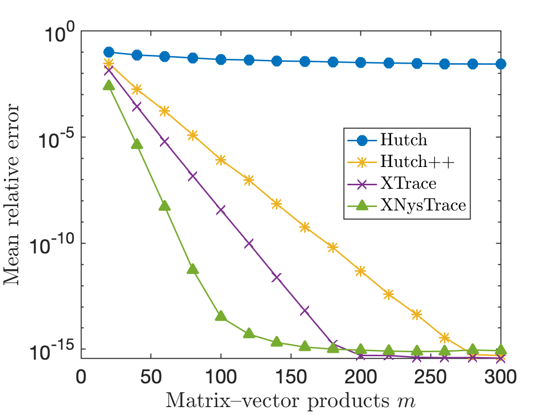
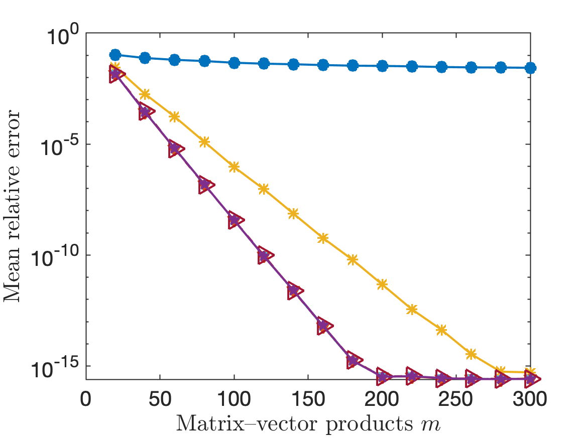
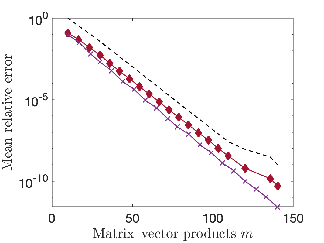
We apply several trace estimators to a psd matrix with exponentially decreasing eigenvalues; see Section 4.1 for the details of the matrix. Figure 1 reports the average error over 1000 trials. The Girard–Hutchinson estimator (Hutch) converges at the Monte Carlo rate, whereas the newer estimators all converge much faster. This improvement comes from variance reduction techniques that exploit the spectral decay. Observe that XTrace and XNysTrace converge exponentially fast at $1.5\times$ and $3\times$ the rate of Hutch++, until reaching machine precision. For a fixed budget of $m$ matvecs, XTrace and XNysTrace can reduce the error by several orders of magnitude compared to Hutch++. Strikingly, the reduction in variance from enforcing exchangeability is almost as significant as the reduction in variance from using a low-rank approximation as a control variate.

Figure 1: Exploiting spectral decay. Average error of trace estimators applied to a (synthetic) psd matrix with exponentially decreasing eigenvalues. See Section 1.3.1.

1.3.2 Computing partition functions

Our second experiment shows how the advantages of using exchangeable estimators persist in a scientific application.

We apply several trace estimators to compute the partition function for a quantum system

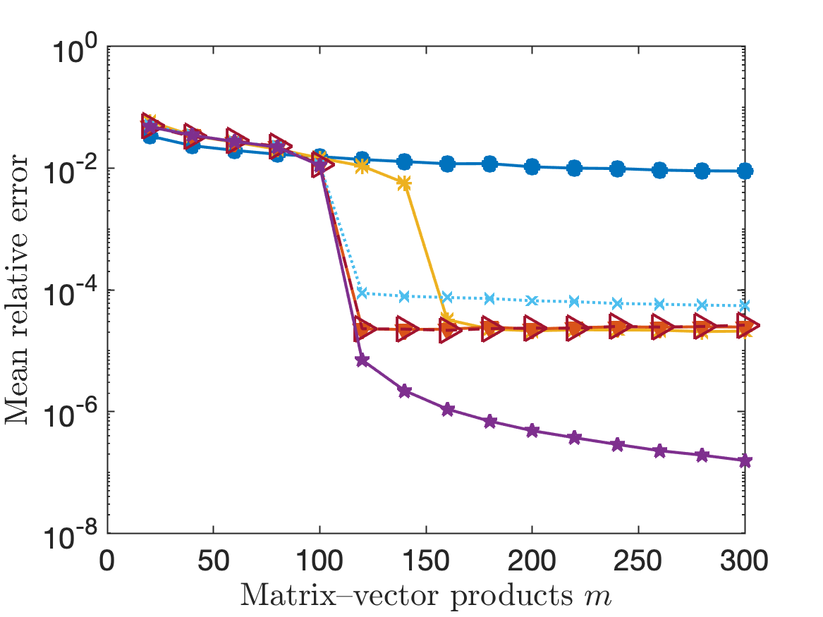
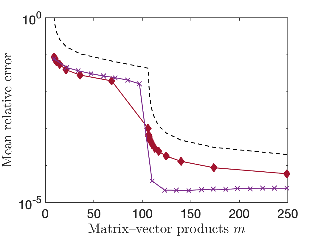
$$Z(\beta)\coloneqq\operatorname{tr}\exp(-\beta\boldsymbol{H}),$$

where $\boldsymbol{H}$ is a symmetric Hamiltonian matrix and $\beta>0$ is an inverse temperature. Specifically, we consider the Hamiltonian matrix $\boldsymbol{H}$ for the tranverse-field Ising model on $18$ sites, which has dimension $N=2^{18}=262\,144$. See Section 4.3 for details on the matrix $\boldsymbol{H}$ and the partition function $Z(\beta)$. To evaluate matvecs with $\exp(-\beta\boldsymbol{H})$, we use the code of Higham [18] that implements an adaptive polynomial approximation [2]. For this problem, each matvec is expensive, occupying over 98% of the total computation time for XTrace with $m=100$. Thus, the cost of all the trace estimators is dominated by the computational cost of the matvecs.

Figure 2: Computing a partition function. Average error of trace estimators applied to the partition function of the transverse-field Ising model. See Section 1.3.2.

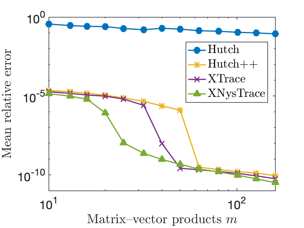
Figure 2 reports the mean estimation error over 100 trials. With just $m=10$ matvecs, all the variance-reduced methods achieve errors that are $5$ orders of magnitude smaller than the Girard–Hutchinson estimator. Furthermore, XTrace and XNysTrace converge more quickly than Hutch++ as we increase the number of matvecs. For example, with $m=40$ matvecs, XTrace is 240$\times$ more accurate, and XNysTrace is 2400$\times$ more accurate. The disparate performance of the three variance-reduced methods is a consequence of the eigenvalues of the matrix $\exp(-\beta\boldsymbol{H})$, which drop sharply from eigenvalue $19$ to $20$: $\lambda_{19}/\lambda_{20}=4600$. Because XNysTrace, XTrace, and Hutch++ use approximation ranks of roughly $m$, $m/2$, and $m/3$, it takes these algorithms 20, 40, and 60 matvecs to capitalize on this eigenvalue drop, leading to the significant differences in performance between the methods.

1.4 Theoretical guarantees

To explain the excellent performance of the exchangeable estimators, we establish detailed theoretical guarantees. For theoretical convenience, our analysis uses standard normal test vectors. As a consequence, we can deliver explicit constants that allow us to make meaningful comparisons among the methods.

Theorem 1.1 (Variance bounds).

Let $\boldsymbol{A}\in{}^{N\times N}$ be a square matrix. Fix the number of matvecs: $m\geq 8$. The Hutch++, XTrace, and XNysTrace estimators are unbiased estimators of the trace. With standard normal test vectors $\boldsymbol{\omega}\sim\textsc{normal}(\boldsymbol{0},\mathbf{I})$, these estimators satisfy the variance bounds

$$\bigl{(}\mathbb{E}\bigl{|}\widehat{\operatorname{tr}}_{\rm H++}-\operatorname{tr}\boldsymbol{A}\bigr{|}^{2}\bigr{)}^{\tfrac{1}{2}} \leq\makebox[0.0pt][r]{}\min_{\color[rgb]{0,0,1}r\leq m/3-2}\,\Biggl{(}\sqrt{2}\frac{\lVert\boldsymbol{A}-\left\llbracket\boldsymbol{A}\right\rrbracket_{r}\rVert_{\rm F}}{\sqrt{m/3-r-1}}\Biggr{)};$$

$$\bigl{(}\mathbb{E}\bigl{|}\widehat{\operatorname{tr}}_{\rm X}-\operatorname{tr}\boldsymbol{A}\bigr{|}^{2}\bigr{)}^{\tfrac{1}{2}} \leq\makebox[0.0pt][r]{$\sqrt{m}$}\min_{\color[rgb]{0,0,1}r\leq m/2-4}\,\Biggl{(}2\frac{\lVert\boldsymbol{A}-\left\llbracket\boldsymbol{A}\right\rrbracket_{r}\rVert}{\sqrt{m/2-r-3}}+2\mathrm{e}\frac{\lVert\boldsymbol{A}-\left\llbracket\boldsymbol{A}\right\rrbracket_{r}\rVert_{\rm F}}{m/2-r-3}\Biggr{)};$$

$$\bigl{(}\mathbb{E}\bigl{|}\widehat{\operatorname{tr}}_{\rm XN}-\operatorname{tr}\boldsymbol{A}\bigr{|}^{2}\bigr{)}^{\tfrac{1}{2}} \leq\makebox[0.0pt][r]{$m$}\min_{\color[rgb]{0,0,1}r\leq m-6}\,\Biggl{(}\sqrt{8}\frac{\lVert\boldsymbol{A}-\left\llbracket\boldsymbol{A}\right\rrbracket_{r}\rVert}{m-r-5}+\sqrt{2}\frac{\lVert\boldsymbol{A}-\left\llbracket\boldsymbol{A}\right\rrbracket_{r}\rVert_{\rm F}}{(m-r-5)^{3/2}}$$

$$\qquad\qquad\qquad\qquad\qquad+5\mathrm{e}^{2}\frac{\lVert\boldsymbol{A}-\left\llbracket\boldsymbol{A}\right\rrbracket_{r}\rVert_{\ast}}{(m-r-5)^{2}}\Biggr{)}.$$

These formulas involve the Frobenius norm $\left\|\cdot\right\|_{\rm F}$, the spectral norm $\left\|\cdot\right\|$, and the trace/nuclear norm $\left\|\cdot\right\|_{*}$. The matrix $\left\llbracket\boldsymbol{A}\right\rrbracket_{r}$ is a simultaneous best rank-$r$ approximation of $\boldsymbol{A}$ in these norms.

In addition, for each of these three methods, it suffices to use $m=\mathcal{O}(\eta^{-1/2})$ matvecs to achieve the variance bound

(10) $$\operatorname{Var}[\widehat{\operatorname{tr}}]=\operatorname{\mathbb{E}}\big{[}|\widehat{\operatorname{tr}}-\operatorname{tr}\boldsymbol{A}|^{2}\big{]}\leq\eta\lVert\boldsymbol{A}\rVert_{\ast}^{2}\quad\text{for $\eta\in(0,1)$.}$$

The proof of Theorem 1.1 appears in Section 5.

As the number $m$ of matvecs increases, Theorem 1.1 ensures that the variance of XTrace, XNysTrace, and Hutch++ decreases at a rate of $\mathcal{O}(1/m^{2})$. Therefore, these algorithms are all superior to the Girard–Hutchinson estimator, whose variance decreases at the Monte Carlo rate $\Theta(1/m)$.

Theorem 1.1 also demonstrates the advantage of XTrace and XNysTrace for matrices whose singular values decay rapidly. This benefit is visible from the error bounds because they allow for larger values $r$ of the approximation rank. As an example, consider a psd matrix $\boldsymbol{A}$ whose eigenvalues have exponential decay with rate $\alpha\in(0,1):$

$$\lambda_{i}(\boldsymbol{A})\leq\alpha^{i}\quad\text{for }i=1,2,3,\ldots.$$

The errors of Hutch++, XTrace, and XNysTrace decay like

$$\bigl{(}\mathbb{E}\bigl{|}\widehat{\operatorname{tr}}_{\rm H++}-\operatorname{tr}\boldsymbol{A}\bigr{|}^{2}\bigr{)}^{1/2} \leq\makebox[0.0pt][r]{}\,C_{1}(\alpha)\,\alpha^{\color[rgb]{0,0,1}m/3};$$

$$\bigl{(}\mathbb{E}\bigl{|}\widehat{\operatorname{tr}}_{\rm X}-\operatorname{tr}\boldsymbol{A}\bigr{|}^{2}\bigr{)}^{1/2} \leq\sqrt{m}\,C_{2}(\alpha)\,\alpha^{\color[rgb]{0,0,1}m/2};$$

$$\bigl{(}\mathbb{E}\bigl{|}\widehat{\operatorname{tr}}_{\rm XN}-\operatorname{tr}\boldsymbol{A}\bigr{|}^{2}\bigr{)}^{1/2} \leq\makebox[0.0pt][r]{$m$}\,C_{3}(\alpha)\,\alpha^{\color[rgb]{0,0,1}m}.$$

For this class of matrix, XTrace converges exponentially fast at $1.5\times$ the rate of Hutch++, and XNysTrace converges exponentially fast at $3\times$ the rate of Hutch++. This is precisely the behavior we observe in Fig. 1.

1.5 Benefits

In summary, the XTrace and XNysTrace estimators have several desirable features as compared with previous approaches.

1. Higher accuracy: For a budget of $m$ matvecs, XTrace and XNysTrace often yield errors that are orders of magnitude smaller than Hutch++.

2. Efficient algorithms: We have designed implementations of XTrace and XNysTrace that only require $m$ matvecs plus $\mathcal{O}(m^{2}N)$ arithmetic operations, which is the same computational cost as Hutch++.

3. Error estimation: We can equip the XTrace and XNysTrace estimators with reliable error estimates.

1.6 A brief history of stochastic trace estimation

Girard wrote the first paper [14] on stochastic trace estimation, in which he proposed the estimator Eq. 2 with test vectors drawn uniformly from a Euclidean sphere. His goal was to develop an efficient way to perform generalized cross-validation for smoothing splines. Hutchinson [19] suggested using random sign vectors instead: $\boldsymbol{\omega}\sim\textsc{uniform}\{\pm 1\}^{N}$. See [25, §4] for further details.

In the last five years, researchers have developed far more efficient methods for trace estimation by incorporating variance reduction techniques. In 2017, Saibaba, Alexanderian, and Ipsen [31] proposed a biased estimator that outputs the trace of a low-rank approximation as a surrogate for $\operatorname{tr}\boldsymbol{A}$. Around the same time, Gambhir, Stathopoulos, and Orginos [12] proposed a hybrid estimator, similar to Hutch++, that outputs the trace of a low-rank approximation, $\operatorname{tr}\boldsymbol{\widehat{A}}$, plus a Girard–Hutchinson estimate for $\operatorname{tr}(\boldsymbol{A}-\boldsymbol{\widehat{A}})$. The paper [23] of Lin contains related ideas.

In 2021, Meyer et al. [26] distilled the ideas from [12, 23] to develop the Hutch++ algorithm. They proved that Hutch++ satisfies a worst-case variance bound of $\mathcal{O}(1/m^{2})$. Meyer et al. also proposed a version of Hutch++ that needs only a single pass over the input matrix. The follow-up paper [20] sharpens the analysis of the single-pass algorithm.

Persson, Cortinovis, and Kressner [28] have introduced several refinements to the Hutch++ estimator. Their first improvement adaptively apportions test vectors between approximating the matrix and estimating the trace of the residual in order to meet an error tolerance. Their second contribution is Nyström++, a version of Hutch++ for psd matrices that uses Nyström approximation.

XTrace and XNysTrace build on the previous strategies of variance reduction using low-rank approximation. However, XTrace and XNysTrace take a step forward by also enforcing the exchangeability principle. These algorithms push the ideas of Hutch++ and Nyström++ to their limit by using all the test vectors for low-rank approximation and all the test vectors for residual trace estimation.

To conclude, let us mention two techniques designed for computing the trace of a standard matrix function (that is, $\operatorname{tr}f(\boldsymbol{A})$). First, stochastic Lanczos quadrature [34] approximates the spectral density of $\boldsymbol{A}$, from which estimates of $\operatorname{tr}f(\boldsymbol{A})$ for any function $f(\cdot)$ are immediately accessible. See [8] for a recent overview of stochastic Lanczos quadrature and related ideas. As a second approach, when the matvecs $\boldsymbol{\omega}\mapsto f(\boldsymbol{A})\boldsymbol{\omega}$ are computed using a Krylov subspace method [17, §13.2], the paper [7] recommends reuse of the matvecs from the Krylov subspace method for the purpose of trace estimation.

1.7 Reproducible research

Optimized MATLAB R2022b implementations of our algorithms as well as code to reproduce the experiments in this paper can be found online at https://github.com/eepperly/XTrace.

1.8 Outline

The remainder of the paper is organized as follows. Section 2 describes efficient implementations for XTrace, XNysTrace, and the diagonal estimator XDiag. Section 3 discusses error estimation and adaptive stopping, Section 4 presents numerical experiments, and Section 5 proves our theoretical results.

1.9 Notation

Matrices and vectors are denoted by capital and lowercase bold letters. The $i$th column of $\boldsymbol{B}$ is expressed as $\boldsymbol{b}_{i}$, and the $(i,j)$th entry of $\boldsymbol{B}$ is $b_{ij}$. For a matrix $\boldsymbol{B}$, we form a matrix $\boldsymbol{B}_{-i}$ by deleting the $i$th column from $\boldsymbol{B}$. Similarly, we form $\boldsymbol{B}_{-ij}$ by deleting the $i$th and $j$th columns. We work with the spectral norm $\left\|\cdot\right\|$, the Frobenius norm $\left\|\cdot\right\|_{\rm F}$, and the trace/nuclear norm $\left\|\cdot\right\|_{*}$. The symbol $\left\llbracket\boldsymbol{B}\right\rrbracket_{r}$ denotes a (simultaneous) best rank-$r$ approximation of $\boldsymbol{B}$ with respect to any unitarily invariant norm.

2 Efficient implementation of exchangeable trace estimators

This section works through some issues that arise in the implementation of the XTrace and XNysTrace estimators. Sections 2.1 and 2.2 show how to implement the new estimators efficiently using insights from numerical linear algebra. Section 2.3 discusses a method of renormalizing the test vectors that improves the accuracy of XTrace and XNysTrace. Section 2.4 develops the XDiag estimator.

2.1 Computing XTrace

In this section, we develop an efficient implementation of the XTrace estimator from Section 1.2.1. Recall that $\boldsymbol{A}\in{}^{N\times N}$ is a general square matrix, and introduce the test matrix $\boldsymbol{\Omega}=\begin{bmatrix}\boldsymbol{\omega}_{1}&\ldots&\boldsymbol{\omega}_{m/2}\end{bmatrix}\in{}^{N\times(m/2)}$.

First, we form the matrix product $\boldsymbol{A}\boldsymbol{\Omega}$ and compute the orthogonal decomposition $\boldsymbol{A}\boldsymbol{\Omega}=\boldsymbol{Q}\boldsymbol{R}$. Following [10, App. A.2], we make the critical observation that the basis matrix $\boldsymbol{Q}_{(i)}=\operatorname{orth}(\boldsymbol{A}\boldsymbol{\Omega}_{-i})$ is related to the full basis matrix $\boldsymbol{Q}$ by a rank-one update:

(11) $$\boldsymbol{Q}_{(i)}^{\vphantom{*}}\boldsymbol{Q}^{*}_{(i)}=\boldsymbol{Q}\big{(}\mathbf{I}-\boldsymbol{s}_{i}^{\vphantom{*}}\boldsymbol{s}_{i}^{*}\big{)}\boldsymbol{Q}^{*}\quad\text{where}\quad\boldsymbol{R}_{-i}^{*}\boldsymbol{s}_{i}=\boldsymbol{0}\quad\text{and}\quad\left\|\boldsymbol{s}_{i}\right\|_{\ell_{2}}=1.$$

Thus, the rank-one update requires a unit vector $\boldsymbol{s}_{i}\in{}^{N}$ in the null space of $\boldsymbol{R}_{-i}^{*}$.

Let us exhibit an efficient algorithm that simultaneously computes all the vectors $\boldsymbol{s}_{i}$ for $1\leq i\leq m/2$. We argue that the matrix $\boldsymbol{S}=\begin{bmatrix}\boldsymbol{s}_{1}&\dots&\boldsymbol{s}_{m/2}\end{bmatrix}$ can be represented as

(12) $$\boldsymbol{S}=(\boldsymbol{R}^{*})^{-1}\boldsymbol{D},$$

where the diagonal matrix $\boldsymbol{D}$ chosen to enforce the normalization of the columns of $\boldsymbol{S}$. Indeed, since $\boldsymbol{R}^{*}\boldsymbol{S}=\boldsymbol{D}$ is diagonal, the $i$th column of $\boldsymbol{R}_{-i}^{*}\boldsymbol{S}$ is the zero vector. We reach the desired conclusion $\boldsymbol{R}_{-i}^{*}\boldsymbol{s}_{i}=\boldsymbol{0}$.

In summary, given the full basis $\boldsymbol{Q}$, we can use Eq. 12 to compute all the vectors $\boldsymbol{s}_{i}$ needed to construct the orthogonal projectors $\boldsymbol{Q}_{(i)}^{\vphantom{*}}\boldsymbol{Q}_{(i)}^{\ast}$ for $1\leq i\leq m/2$ appearing in Eq. 11. This calculation requires just $\mathcal{O}(m^{3})$ operations, which is dominated by the cost of solving $m/2$ triangular linear systems. It follows that the XTrace estimator can be computed in just $\mathcal{O}(m^{2}N)$ operations, which is the same asymptotic cost as Hutch++. For full details, see the efficient MATLAB implementation in the supplementary materials LABEL:list:xtrace.

2.2 Computing XNysTrace

We can design a similar method to compute the XNysTrace estimator Eq. 9 efficiently. Let $\boldsymbol{A}\in{}^{N\times N}$ be a psd matrix and define the test matrix $\boldsymbol{\Omega}=\begin{bmatrix}\boldsymbol{\omega}_{1}&\dots&\boldsymbol{\omega}_{m}\end{bmatrix}$.

As before, we compute the orthogonal decomposition $\boldsymbol{A}\boldsymbol{\Omega}=\boldsymbol{Q}\boldsymbol{R}$. We can express the Nyström approximation Eq. 7 in the form

$$\boldsymbol{A}\left\langle\boldsymbol{\Omega}\right\rangle=\boldsymbol{Q}\boldsymbol{R}\boldsymbol{H}^{-1}\boldsymbol{R}^{*}\boldsymbol{Q}^{*},$$

where $\boldsymbol{H}=\boldsymbol{\Omega}^{*}\boldsymbol{A}\boldsymbol{\Omega}$. After deleting the $i$th column from $\boldsymbol{\Omega}$, the resulting Nyström approximation satisfies

(13) $$\boldsymbol{A}\left\langle\boldsymbol{\Omega}_{-i}\right\rangle=\boldsymbol{Q}\boldsymbol{R}_{-i}^{\vphantom{*}}\boldsymbol{H}_{(i)}^{-1}\boldsymbol{R}_{-i}^{*}\boldsymbol{Q}^{*},$$

where $\boldsymbol{H}_{(i)}$ is $\boldsymbol{H}$ upon deletion of its $i$th row and column. To compute $\boldsymbol{A}\left\langle\boldsymbol{\Omega}_{-i}\right\rangle$ efficiently, we recognize that Eq. 13 can be expressed as a rank-one update:

(14) $$\boldsymbol{A}\left\langle\boldsymbol{\Omega}_{-i}\right\rangle=\boldsymbol{Q}\boldsymbol{R}\left(\boldsymbol{H}^{-1}-\frac{\boldsymbol{H}^{-1}\mathbf{e}_{i}^{\vphantom{*}}\mathbf{e}_{i}^{*}\boldsymbol{H}^{-1}}{\mathbf{e}_{i}^{*}\boldsymbol{H}^{-1}\mathbf{e}_{i}^{\vphantom{*}}}\right)\boldsymbol{R}^{*}\boldsymbol{Q}^{*}.$$

Taking advantage of the rank-one update formula Eq. 14, we can form the XNysTrace estimator using just $m$ matvecs and $\mathcal{O}(m^{2}N)$ post-processing operations. An efficient MATLAB implementation appears in the supplementary materials LABEL:list:xnystrace, which incorporates several additional tricks taken from [22, 33] to improve its numerical stability.

2.3 Normalization of test vectors

For the best general performance of XTrace and XNysTrace, we recommend a modification of the basic XTrace and XNysTrace procedure in which the test vectors are orthogonalized against the low-rank approximation $\boldsymbol{Q}_{(i)}^{\vphantom{*}}\boldsymbol{Q}_{(i)}^{*}\boldsymbol{A}$ or $\boldsymbol{A}\langle\boldsymbol{\Omega}_{-i}\rangle$ and renormalized. This renormalization strategy proceeds as follows: First, we draw the test vectors from a spherically symmetric distribution, such as $\boldsymbol{\omega}\sim\textsc{normal}(\boldsymbol{0},\mathbf{I})$. We use these test vectors to form the matrix $\boldsymbol{Q}_{(i)}$ or Nyström approximation $\boldsymbol{A}\langle\boldsymbol{\Omega}_{-i}\rangle$. Second, when computing the basic trace estimates, we normalize the test vectors. In XTrace, we compute

$$\boldsymbol{\mu}_{i}\coloneqq\bigl{(}\mathbf{I}-\boldsymbol{Q}_{(i)}\boldsymbol{Q}_{(i)}^{*}\bigr{)}\boldsymbol{\omega}_{i}\quad\text{and}\quad\boldsymbol{\nu}_{i}\coloneqq\sqrt{N-\operatorname{rank}(\boldsymbol{Q}_{(i)})}\cdot\frac{\boldsymbol{\mu}_{i}}{\left\|\boldsymbol{\mu}_{i}\right\|_{\ell_{2}}}.$$

To obtain the $i$th trace estimate, we form

$$\widehat{\operatorname{tr}}_{i}\coloneqq\operatorname{tr}\big{(}\boldsymbol{Q}_{(i)}^{*}(\boldsymbol{A}\boldsymbol{Q}_{(i)}^{\vphantom{*}})\big{)}+\boldsymbol{\nu}_{i}^{*}\big{(}\boldsymbol{A}\boldsymbol{\nu}_{i}^{\vphantom{*}}\big{)}.$$

For XNysTrace, we set

$$\boldsymbol{P}_{(i)}\coloneqq\operatorname{orth}\boldsymbol{\Omega}_{-i},\>\>\boldsymbol{\mu}_{i}\coloneqq(\mathbf{I}-\boldsymbol{P}_{(i)}\boldsymbol{P}_{(i)}^{*})\boldsymbol{\omega}_{i},\>\>\text{and}\>\>\boldsymbol{\nu}_{i}\coloneqq\sqrt{N-\operatorname{rank}(\boldsymbol{P}_{(i)})}\cdot\frac{\boldsymbol{\mu}_{i}}{\left\|\boldsymbol{\mu}_{i}\right\|_{\ell_{2}}}.$$

Then define the basic trace estimates

$$\widehat{\operatorname{tr}}_{i}\coloneqq\operatorname{tr}\boldsymbol{A}\langle\boldsymbol{\Omega}_{-i}\rangle+\boldsymbol{\nu}_{i}^{*}\big{(}\boldsymbol{A}\boldsymbol{\nu}_{i}^{\vphantom{*}}\big{)}.$$

The normalization removes a source of variance related to the random lengths of the vectors $\boldsymbol{\mu}_{i}$, improving the accuracy compared to unnormalized Gaussian test vectors or uniform random vectors on the sphere. We compare this normalization approach against alternative distributions for test vectors in Section 4.2.

2.4 Diagonal estimation

In the spirit of Girard and Hutchinson, the paper [5] of Bekas, Kokiopoulou, and Saad (BKS) develops an estimator for the diagonal of an implicit matrix:

(15) $$\widehat{\boldsymbol{\operatorname{diag}}}_{\rm BKS}=\frac{\sum_{i=1}^{m}\boldsymbol{\omega}_{i}\odot(\boldsymbol{A}\boldsymbol{\omega}_{i})}{\sum_{i=1}^{m}\boldsymbol{\omega}_{i}\odot\boldsymbol{\omega}_{i}}.$$

Here, $\odot$ denotes the entrywise product and the division is performed entrywise. The recent paper [4] proposes a biased estimator for the diagonal, called Diag++, that is inspired by BKS and Hutch++.

We have observed that the exchangeability principle leads to an unbiased diagonal estimator with lower variance. Our diagonal estimator, XDiag, takes the form

$$\boldsymbol{\widehat{\operatorname{diag}}}_{\rm X}=\frac{1}{m/2}\sum_{i=1}^{m/2}\left[\operatorname{diag}\big{(}\boldsymbol{Q}_{(i)}^{\vphantom{*}}(\boldsymbol{Q}_{(i)}^{*}\boldsymbol{A})\big{)}+\frac{\boldsymbol{\omega}_{i}\odot\big{(}\mathbf{I}-\boldsymbol{Q}_{(i)}^{\vphantom{*}}\boldsymbol{Q}_{(i)}^{*}\big{)}(\boldsymbol{A}\boldsymbol{\omega}_{i})}{\boldsymbol{\omega}_{i}\odot\boldsymbol{\omega}_{i}}\right],$$

where $\boldsymbol{Q}_{(i)}$ is defined in Eq. 4. In contrast to XTrace, the XDiag estimator requires matvecs with $\boldsymbol{A}^{*}$ in addition to matvecs with $\boldsymbol{A}$. The same ideas from Section 2.1 allow us to implement XDiag in $\mathcal{O}(m^{2}N)$ operations; an implementation is provided in the supplementary materials (LABEL:list:xdiag).

3 Error estimation and adaptive stopping

Our exchangeable estimators depend on averaging over a family of basic estimators, and we can reuse the basic estimators to compute a reliable posterior approximation for the error (Section 3.1). The error estimate allows us to develop adaptive methods for selecting the number $m$ of matvecs to achieve a specified error tolerance (Section 3.2). These refinements are very important for practical implementations.

3.1 Error estimation

The XTrace and XNysTrace estimators are both formed as averages of individual trace estimates $\widehat{\operatorname{tr}}_{1},\ldots,\widehat{\operatorname{tr}}_{\ell}$ where

$$\widehat{\operatorname{tr}}_{i} =\operatorname{tr}\big{(}\boldsymbol{Q}_{(i)}^{*}\boldsymbol{A}\boldsymbol{Q}_{(i)}^{\vphantom{*}}\big{)}+\boldsymbol{\omega}_{i}^{*}\big{(}\mathbf{I}-\boldsymbol{Q}_{(i)}^{\vphantom{*}}\boldsymbol{Q}_{(i)}^{*}\big{)}\boldsymbol{A}\big{(}\mathbf{I}-\boldsymbol{Q}_{(i)}^{\vphantom{*}}\boldsymbol{Q}_{(i)}^{*}\big{)}\boldsymbol{\omega}_{i}^{\vphantom{*}}, \!\!\ell\coloneqq\frac{m}{2}$$ (XTrace);

$$\widehat{\operatorname{tr}}_{i} =\operatorname{tr}(\boldsymbol{A}\langle\boldsymbol{\Omega}_{-i}\rangle)+\boldsymbol{\omega}_{i}^{*}(\boldsymbol{A}-\boldsymbol{A}\langle\boldsymbol{\Omega}_{-i}\rangle)\boldsymbol{\omega}_{i}^{\vphantom{*}}, \!\!\ell\coloneqq m$$ (XNysTrace).

The scaled variance of the individual trace estimates $\widehat{\operatorname{tr}}_{i}$ provides a useful estimate for the squared error in the trace estimate:

(16) $$\widehat{\mathrm{err}}^{2}\coloneqq\frac{1}{\ell(\ell-1)}\sum_{i=1}^{\ell}\left|\widehat{\operatorname{tr}}_{i}-\widehat{\operatorname{tr}}\right|^{2}\approx\left|\operatorname{tr}(\boldsymbol{A})-\widehat{\operatorname{tr}}\right|^{2}\quad\text{where}\quad\widehat{\operatorname{tr}}=\frac{1}{\ell}\sum_{i=1}^{\ell}\widehat{\operatorname{tr}}_{i}.$$

The next result contains an analysis of this posterior error estimator.

Proposition 3.1 (Error estimate).

The error estimate Eq. 16 satisfies

$$\operatorname{\mathbb{E}}\widehat{\mathrm{err}}^{2}=\frac{1-\operatorname{Cor}(\widehat{\operatorname{tr}}_{1},\widehat{\operatorname{tr}}_{2})}{1+(\ell-1)\operatorname{Cor}(\widehat{\operatorname{tr}}_{1},\widehat{\operatorname{tr}}_{2})}\cdot\operatorname{\mathbb{E}}\left|\operatorname{tr}(\boldsymbol{A})-\widehat{\operatorname{tr}}\right|^{2}.$$

We have written $\operatorname{Cor}(\cdot,\cdot)$ for the correlation of two random variables.

The proof and some additional discussion of the correlation $\operatorname{Cor}(\widehat{\operatorname{tr}}_{1},\widehat{\operatorname{tr}}_{2})$ appears in Section 5.6. In practice, we find that the individual trace estimators have a small positive correlation, so we typically underestimate the true error by a small amount. Thus, the posterior error estimate is a valuable tool. For an illustration, see Fig. 5(a) in Section 4.3.

3.2 Adaptive stopping

In practice, we often wish to choose the number $m$ of matvecs adaptively to estimate $\operatorname{tr}\boldsymbol{A}$ up to a prescribed accuracy level:

$$|\,{\operatorname{tr}(\boldsymbol{A})-\widehat{\operatorname{tr}}}\,|\leq\varepsilon\cdot|\,{\operatorname{tr}\boldsymbol{A}}\,|\quad\text{for $\varepsilon\in(0,1)$.}$$

One simple way to achieve this tolerance is through a doubling strategy:

1. To initialize, collect $m_{0}$ matvecs $\boldsymbol{A}\boldsymbol{\omega}_{1},\ldots,\boldsymbol{A}\boldsymbol{\omega}_{m_{0}}$, and set $j\leftarrow 0$.

2. Use $\boldsymbol{A}\boldsymbol{\omega}_{1},\ldots,\boldsymbol{A}\boldsymbol{\omega}_{m_{j}}$ to form a trace estimate $\widehat{\operatorname{tr}}^{(j)}$ and an error estimate $\widehat{\mathrm{err}}^{(j)}$.

3. If $\widehat{\mathrm{err}}^{(j)}\leq\varepsilon\cdot|\widehat{\operatorname{tr}}^{(j)}|$, then stop.

4. Collect $m_{j}$ additional matvecs $\boldsymbol{A}\boldsymbol{\omega}_{m_{j}+1},\ldots,\boldsymbol{A}\boldsymbol{\omega}_{2m_{j}}$. Set $j\leftarrow j+1$ and $m_{j}\leftarrow 2m_{j-1}$. Go to step 2.

The doubling strategy requires at most twice the optimal number of matvecs to meet the tolerance and maintains the $\mathcal{O}(m^{2}N)$ computational cost of XTrace and XNysTrace. We implement this approach in our experiments to produce Fig. 5(b).

4 Numerical experiments

This section presents a numerical evaluation of XTrace, XNysTrace, and XDiag. Section 4.1 compares different trace estimators on synthetic matrices, Section 4.2 evaluates XNysTrace with different distributions for the test vectors, Section 4.3 applies XTrace and XNysTrace to computations in quantum statistical physics, and Section 4.4 applies XDiag to computations in network science. Throughout this section, we compare different trace estimators based on the error they achieve for a given budget of matvecs; experiments comparing the runtime of different trace estimators is provided in Section SM2. Code to reproduce the experiments can be found at https://github.com/eepperly/XTrace.

4.1 Comparison of trace estimators

The first experiment is designed to compare the accuracy of six trace estimators that each use $m$ matvecs:

• Hutch: The Girard–Hutchinson estimator Eq. 2.

• LRA: The Saibaba et al. [31] estimator (without additional subspace iteration): $\operatorname{tr}\boldsymbol{\widehat{A}}$ where $\boldsymbol{\widehat{A}}=\boldsymbol{Q}\boldsymbol{Q}^{*}\boldsymbol{A}$ and $\boldsymbol{Q}=\operatorname{orth}(\boldsymbol{A}\boldsymbol{\Omega})$.

• The Hutch++ estimator Eq. 3.

• The Nyström++ estimator [28]. We use the implementation provided by the authors of [28], modified to the test vector $\boldsymbol{\omega}\sim\textsc{uniform}\{\pm 1\}^{N}$.

• The XTrace estimator Eq. 6.

• The XNysTrace estimator Eq. 9.

To create a fair comparison, we apply all six estimators using a test matrix whose entries are uniformly random signs: $\boldsymbol{\Omega}\sim\textsc{uniform}\{\pm 1\}^{N\times\ell}$, as was used in Hutch++. The additional benefit for XTrace and XNysTrace of using normalized, spherically symmetric test vectors is explored in Section 4.2. The supplementary materials (Section SM1) contain additional comparisons with the adaptive Hutch++ algorithm of [28]; this comparison requires a more complicated experimental setup.

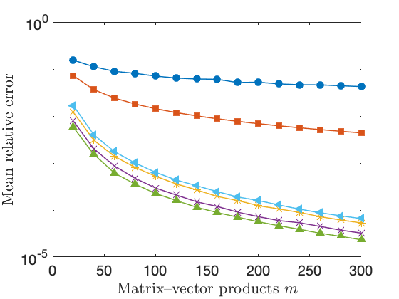
We apply each of these estimators to randomly generated matrices of the form

$$\boldsymbol{A}(\boldsymbol{\lambda})=\boldsymbol{U}\operatorname{diag}(\boldsymbol{\lambda})\boldsymbol{U}^{*}$$

where $\boldsymbol{U}$ is a Haar random orthogonal matrix. We use four choices for the eigenvalues $\boldsymbol{\lambda}$:

• flat: $\boldsymbol{\lambda}=(3-2(i-1)/(N-1):i=1,2,\ldots,N)$.

• poly: $\boldsymbol{\lambda}=(i^{-2}:i=1,2,\ldots,N)$.

• exp: $\boldsymbol{\lambda}=(0.7^{i}:i=0,1,\ldots,N-1)$.

• step: $\boldsymbol{\lambda}=(\underbrace{1,\ldots,1}_{\text{$50$ times}},\underbrace{10^{-3},\ldots,10^{-3}}_{\text{$N-50$ times}})$.

We fix the matrix dimension $N=1000$, and we report the relative error $|{\operatorname{tr}(\boldsymbol{A})}-{\widehat{\operatorname{tr}}}|/\operatorname{tr}(\boldsymbol{A})$ averaged over $1000$ trials.

(a) flat

(b) poly

(c) exp

(d) step

Figure 3: Synthetic instances. Average relative error of trace estimators for matrices with particular spectral profiles using random sign test vectors. See Section 4.1 and Fig. 4.

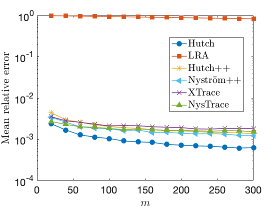
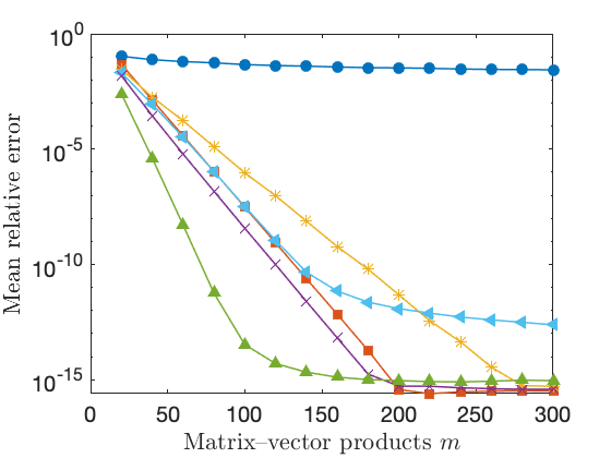
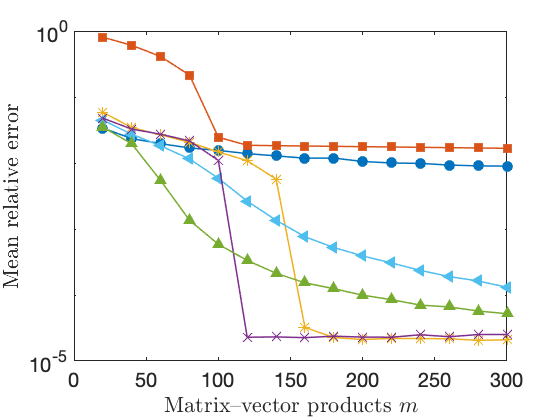
Discussion. The variance-reduced trace estimators dramatically outperform Hutch, except on the flat instance (Fig. 3(a)). The implication is that Hutch only makes sense when estimating the trace of a matrix with a nearly flat spectrum. For the flat instance, the performance of LRA is especially poor because LRA is a biased estimator that substantially underestimates the trace.

Across all the instances, XTrace produces smaller errors than Hutch++, sometimes by orders of magnitude. For the exp instance (Fig. 3(c)), the error of XTrace decays exponentially fast at a rate $1.5\times$ faster than Hutch++. The superiority of XTrace is also visible for the step instance (Fig. 3(d)) where XTrace achieves accuracy $10^{-4}$ with just $m\approx 120$ matvecs, as compared to $m\approx 160$ for Hutch++.

XNysTrace is frequently the most accurate of the trace estimation methods. For the exp instance (Fig. 3(c)), XNysTrace converges at a rate $2\times$ faster than XTrace and Nyström++ and $3\times$ faster than Hutch++. However, XNysTrace (and Nyström++) can exhibit poor performance for matrices that possess a long tail of slowly decreasing eigenvalues (see the step instance in Fig. 3(d)). To understand this phenomenon, observe that the error bounds for XNysTrace depend on the trace/nuclear norm, which is sensitive to slow eigenvalue decay (Theorem 1.1). We can improve the performance by using the normalization approach of Section 2.3, as we detail in the next section.

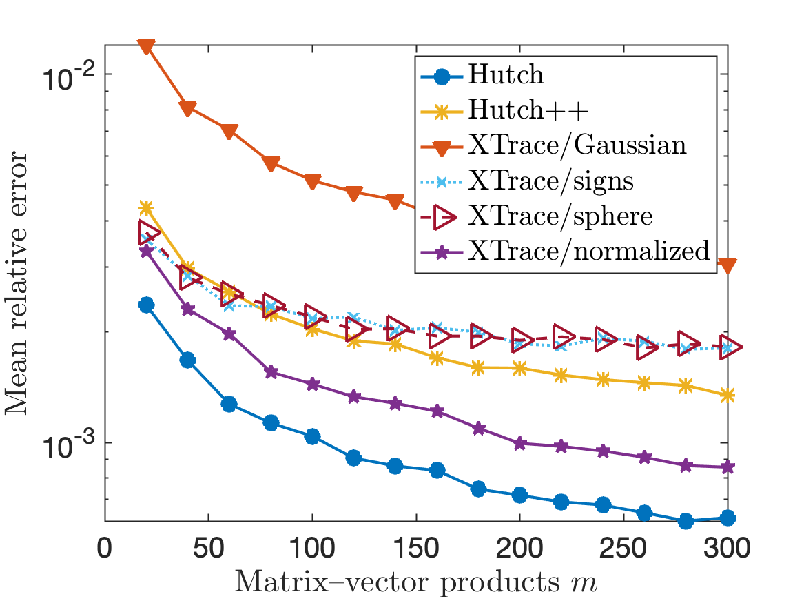
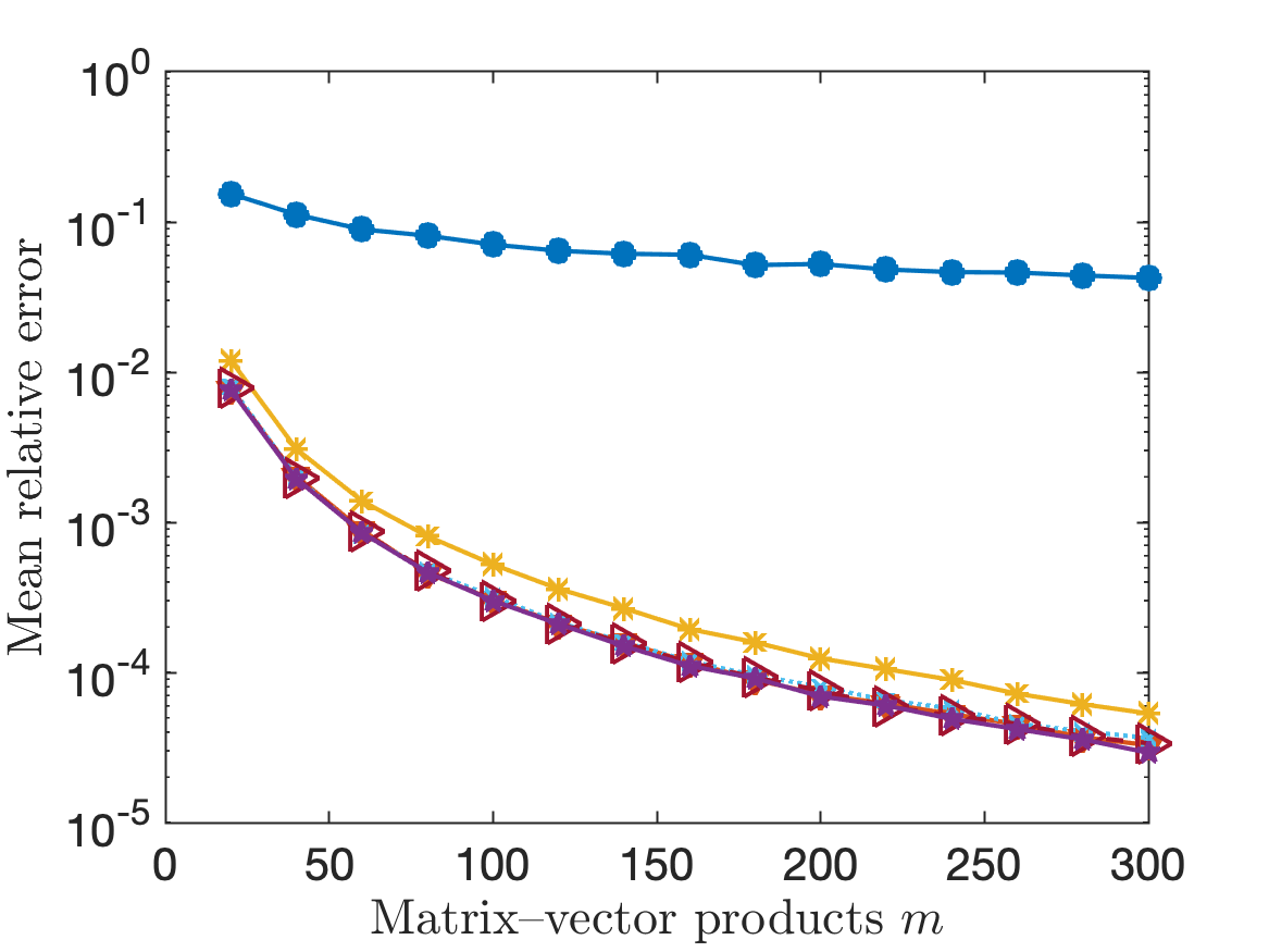
4.2 Choice of test vectors

In Section 2.3, we recommended an implementation of XTrace and XNysTrace that uses rotationally invariant test vectors for low-rank approximation and normalizes the distinguished test vector used for trace estimation.

Figure 4 shows how this method can improve over estimators that lack the normalization step. The figure compares the Girard–Hutchinson estimator, Hutch++, XTrace with normalized test vectors, and XTrace with test vectors from the standard normal distribution $\boldsymbol{\omega}\sim\textsc{normal}(\boldsymbol{0},\mathbf{I})$, the random sign distribution $\boldsymbol{\omega}\sim\textsc{uniform}\{\pm 1\}^{N}$, or the uniform distribution on the sphere $\boldsymbol{\omega}\sim\textsc{uniform}\{\boldsymbol{x}\in{}^{N}:\left\|\boldsymbol{x}\right\|_{\ell_{2}}=\sqrt{N}\}$. The differences between XTrace test vectors are only visible for matrices whose spectra have flat segments, as in the flat and step examples. For these examples, the normalization strategy is conspicuously the best, followed by the uniform sign and uniform sphere distributions, with the standard normal distribution lagging well behind.

(a) flat

(b) poly

(c) exp

(d) step

Figure 4: Normalization of test vectors. The average relative error of the XTrace estimator using normalized test vectors (Section 2.3) as compared with alternative (unnormalized) test vector distributions. See Section 4.2.

4.3 Application: Quantum statistical mechanics

Our next experiment shows the benefits of using XTrace and XNysTrace for an application in quantum physics. To compute a phase diagram, we must evaluate a large number of trace estimators. Our exchangeable estimators reduce the number of matvecs needed to achieve a desired tolerance, and we can use the posterior error estimator to adaptively determine the minimum number $m$ of matvecs.

The average energy of a quantum system with a symmetric Hamiltonian matrix $\boldsymbol{H}\in{}^{N\times N}$ at inverse temperature $\beta>0$ is

$$E(\beta)=\frac{1}{Z(\beta)}\operatorname{tr}[\boldsymbol{H}\exp(-\beta\boldsymbol{H})]\quad\text{where $Z(\beta)=\operatorname{tr}\exp(-\beta\boldsymbol{H})$}.$$

The quantity $Z(\beta)$ is the partition function, introduced in Section 1.3. We observe that $\operatorname{tr}[\boldsymbol{H}\exp(-\beta\boldsymbol{H})]$ and $\operatorname{tr}\exp(-\beta\boldsymbol{H})$ are ideal candidates for estimation using XTrace and XNysTrace, since the matrix exponential leads to rapidly decaying eigenvalues.

We apply XTrace and XNysTrace to compute the partition function and energy for the transverse field Ising model (TFIM) for a periodic 1D chain [29], which is specified by the Hamiltonian matrix

(17) $$\boldsymbol{H}=-\sum_{i=1}^{n}\boldsymbol{Z}_{i}\boldsymbol{Z}_{i+1}-h\sum_{i=1}^{n}\boldsymbol{X}_{i}\in{}^{2^{n}\times 2^{n}}.$$

Here, $\boldsymbol{X}_{i}$ and $\boldsymbol{Z}_{i}$ denote Pauli operators acting on the $i$th site; that is,

$$\boldsymbol{X}_{i}=\mathbf{I}_{2\times 2}^{\otimes(n-i-1)}\otimes\begin{bmatrix}0&1\\ 1&0\end{bmatrix}\otimes\mathbf{I}_{2\times 2}^{\otimes(n-i)},\quad\boldsymbol{Z}_{i}=\mathbf{I}_{2\times 2}^{\otimes(n-i-1)}\otimes\begin{bmatrix}1&0\\ 0&-1\end{bmatrix}\otimes\mathbf{I}_{2\times 2}^{\otimes(n-i)},$$

and $\boldsymbol{Z}_{n+1}=\boldsymbol{Z}_{1}$ by periodicity. The eigenvalues of $\boldsymbol{H}$ are known exactly [24, eqs. (16)–(17)], which allows us to precisely evaluate the error of stochastic estimates of $Z(\beta)=Z(\beta,h)$ and $E(\beta)=E(\beta,h)$. Before applying stochastic trace estimation, we shift the Hamiltonian matrix by a constant $b=(1+h)n$ so that $\boldsymbol{H}+b\mathbf{I}$ is positive semidefinite.

(a)

(b)

Figure 5: Quantum statistical mechanics. Left: Mean relative error (solid lines) and mean posterior error estimates (dashed lines) when computing the partition function $Z(\beta=0.6,h=10)$. Right: Average energy $E(\beta,h)/n$ per site for $\beta,h\in[10^{-1},10^{1}]$ as computed by XNysTrace. See Section 4.3.

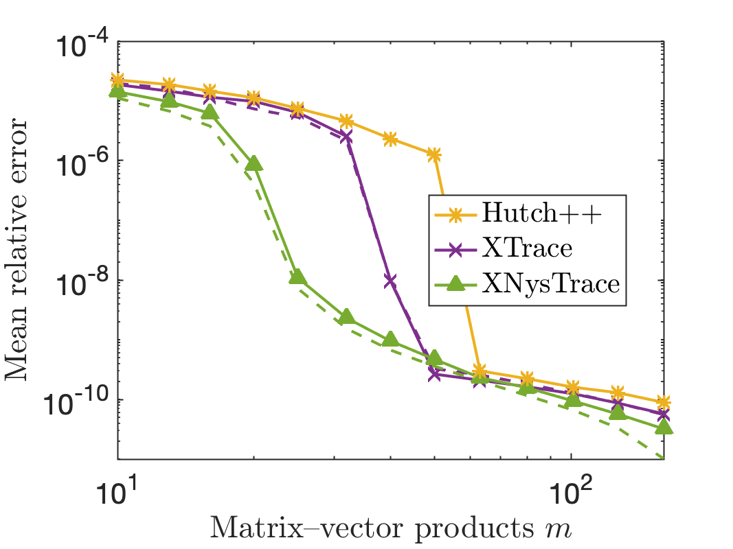
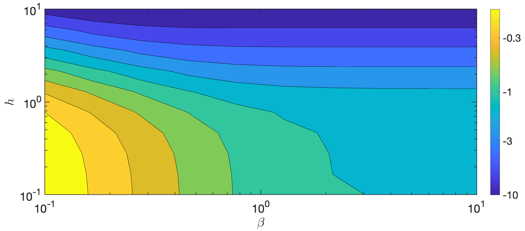
Figure 5(a) shows the errors of Hutch++, XTrace, and XNysTrace when computing the partition function $Z(\beta,h)$ of the TFIM with $n=18$, $h=10$, and $\beta=0.6$; this is the same setting as in Fig. 2. (The Girard–Hutchinson estimator is omitted because the error is four orders of magnitude larger than the other methods.) The thick lines indicate the average errors over 10 trials, while the dashed lines (for XTrace and XNysTrace) indicate the average error estimates introduced in Section 3.1. We observe that the error estimates closely track the true errors, differing by a factor of at most $3.2$.

Figure 5(b) shows the average energy $E(\beta,h)/n$ per site for parameters $\beta,h\in[10^{-1},10^{1}]$, up to a relative error of $10^{-3}$. We compute the energy by using XNysTrace, together with the doubling strategy from Section 3.2. To ensure the robustness of the doubling strategy, we use a slightly stricter tolerance $\varepsilon=10^{-4}$ than our desired accuracy of $10^{-3}$.

4.4 Application: Networks

One of the basic problems in network science is to measure the centrality of each node in a graph. We focus on two centrality measures, which can be defined in terms of the adjacency matrix $\boldsymbol{M}$:

1. The number of triangles [1] incident on node $i$ is given by $\triangle_{i}(\boldsymbol{M})=\tfrac{1}{2}(\boldsymbol{M}^{3})_{ii}$.

2. The subgraph centrality [11] of node $i$ is defined as $\mathrm{SC}_{i}\coloneqq(\exp(\boldsymbol{M}))_{ii}$.

Both centrality measures are the diagonal entries of functions of the adjacency matrix.

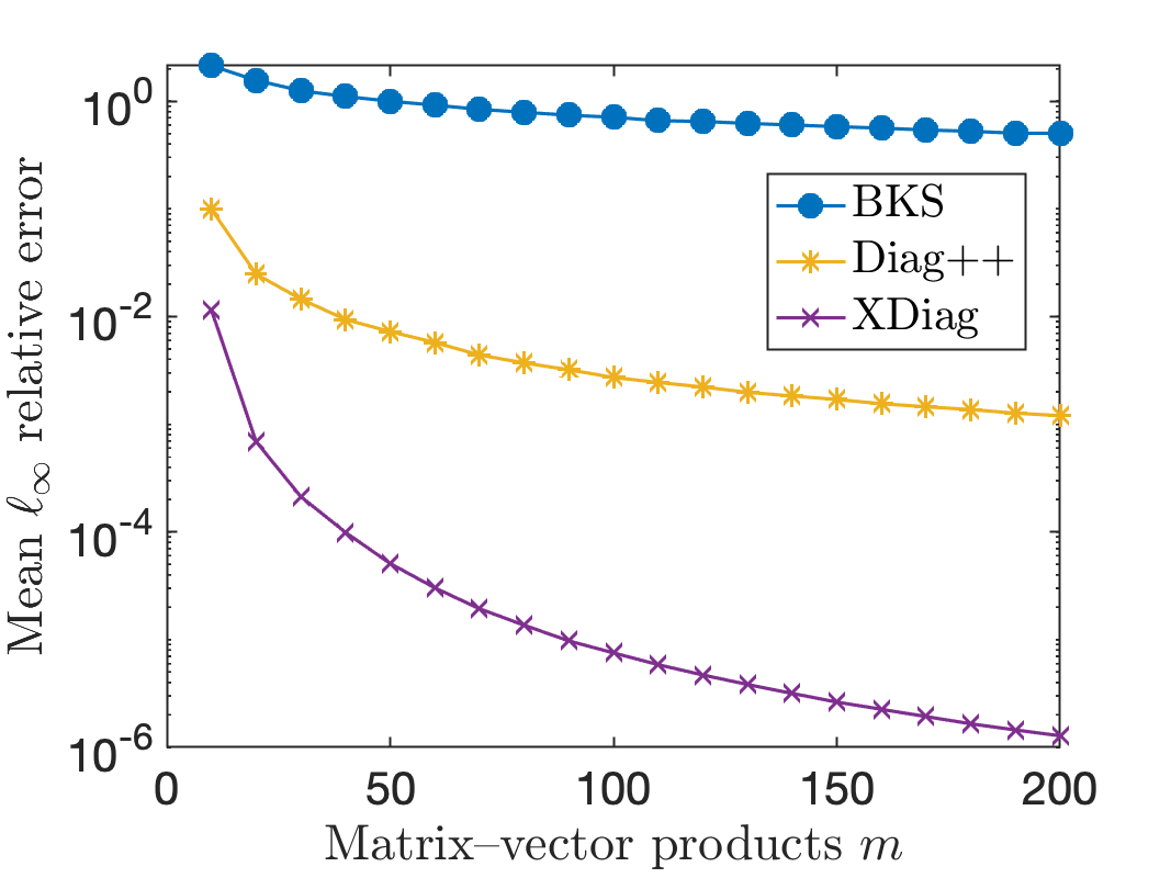
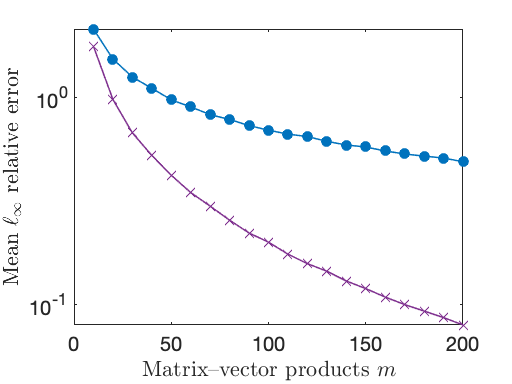
Using the BKS, Diag++, and XDiag diagonal estimators, we estimate these centrality measures for the protein–protein interaction network $\boldsymbol{M}\in{}^{2361\times 2361}$ for budding yeast [6], available in the SuiteSparse collection [9]. (Following [4], Diag++ is omitted for the triangle problem because $\boldsymbol{M}^{3}/2$ is not psd.) The matrix $\boldsymbol{M}^{3}/2$ has modest spectral decay ($\sigma_{1}/\sigma_{100}=40$) and the matrix $\exp(\boldsymbol{M})$ has significant spectral decay ($\sigma_{1}/\sigma_{100}=10^{6}$). We evaluate the quality of our estimates using the relative $\ell_{\infty}$ error

$$\operatorname{error}(\boldsymbol{\widehat{\operatorname{diag}}})\coloneqq\frac{\max_{1\leq i\leq N}|a_{ii}-\widehat{\operatorname{diag}}_{i}|}{\max_{1\leq i\leq N}|a_{ii}|},$$

averaged over 1000 trials. Figure 6 shows the results. For the subgraph centrality problem after $m=200$ matvecs, XDiag is more accurate than BKS by five orders of magnitude and more accurate than Diag++ by three orders of magnitude.

(a) Subgraph centralities $\operatorname{SC}_{i}(\boldsymbol{M})$

(b) Numbers of triangles $\triangle_{i}(\boldsymbol{M})$

Figure 6: Networks. Mean error of BKS diagonal estimator and XDiag for the subgraph centralities (left) and triangle numbers (right) for the yeast graph. See Section 4.4.

5 Theoretical analysis

In this final section, we prove Theorem 1.1, which provides refined error bounds for three trace estimators, and we prove Proposition 3.1, which describes the behavior of the posterior error estimator.

5.1 XTrace variance bound

To begin, let us establish an initial variance bound for the XTrace estimator. This result shows that the variance depends on the error in a low-rank approximation of the input matrix. Later, we will bound these errors using standard results for the randomized SVD.

Proposition 5.1 (XTrace error).

Fix $\boldsymbol{A}\in{}^{N\times N}$, and consider the XTrace estimator $\widehat{\operatorname{tr}}_{\rm X}$ defined in Eq. 6 with a test matrix $\boldsymbol{\Omega}=\begin{bmatrix}\boldsymbol{\omega}_{1}&\dots&\boldsymbol{\omega}_{m/2}\end{bmatrix}$ consisting of $m/2$ standard normal test vectors. The estimator is unbiased: $\operatorname{\mathbb{E}}\widehat{\operatorname{tr}}_{\rm X}=\operatorname{tr}\boldsymbol{A}$. Moreover, the variance satisfies

$$\operatorname{Var}[\widehat{\operatorname{tr}}_{\rm X}]=\mathbb{E}\,\bigl{|}\widehat{\operatorname{tr}}_{\rm X}-\operatorname{tr}\boldsymbol{A}\bigr{|}^{2} \leq\frac{2}{m/2}\mathbb{E}\bigl{\lVert}\big{(}\mathbf{I}-\boldsymbol{Q}_{(1)}\boldsymbol{Q}_{(1)}^{*}\big{)}\boldsymbol{A}\rVert^{2}_{\rm F}+4\,\mathbb{E}\,\bigl{\lVert}\big{(}\mathbf{I}-\boldsymbol{Q}_{(12)}\boldsymbol{Q}_{(12)}^{*}\big{)}\boldsymbol{A}\bigr{\rVert}^{2},$$

where $\boldsymbol{Q}_{(i)}=\operatorname{orth}(\boldsymbol{A}\boldsymbol{\Omega}_{-i})$ and $\boldsymbol{Q}_{(ij)}=\operatorname{orth}(\boldsymbol{A}\boldsymbol{\Omega}_{-ij})$.

Proof 5.2.

For all indices $1\leq i,j\leq m/2$, we abbreviate the orthogonal projectors $\boldsymbol{\Pi}_{i}\coloneqq\boldsymbol{Q}_{(i)}^{\phantom{*}}\boldsymbol{Q}_{(i)}^{*}$ and $\boldsymbol{\Pi}_{ij}\coloneqq\boldsymbol{Q}_{(ij)}^{\phantom{*}}\boldsymbol{Q}_{(ij)}^{*}$. Note that $\boldsymbol{\omega}_{i}$ is independent from $\boldsymbol{\Pi}_{i}$, while $(\boldsymbol{\omega}_{i},\boldsymbol{\omega}_{j})$ is independent from $\boldsymbol{\Pi}_{ij}$.

For each $1\leq i\leq m/2$, we can check that the basic estimator $\widehat{\operatorname{tr}}_{i}$ defined in Eq. 5 is unbiased. To do so, condition on $\boldsymbol{\Omega}_{-i}$ and average over $\boldsymbol{\omega}_{i}$ to arrive at the identity

(18) $$\begin{split}\mathbb{E}\bigl{[}\widehat{\operatorname{tr}}_{i}\,\big{|}\,\boldsymbol{\Omega}_{-i}\bigr{]}&=\mathbb{E}\bigl{[}\operatorname{tr}(\boldsymbol{\Pi}_{i}\boldsymbol{A}\boldsymbol{\Pi}_{i})+\boldsymbol{\omega}_{i}^{*}(\mathbf{I}-\boldsymbol{\Pi}_{i})\boldsymbol{A}(\mathbf{I}-\boldsymbol{\Pi}_{i})\boldsymbol{\omega}_{i}\,\big{|}\,\boldsymbol{\Omega}_{-i}\bigr{]}\\ &=\mathbb{E}\bigl{[}\operatorname{tr}(\boldsymbol{\Pi}_{i}\boldsymbol{A}\boldsymbol{\Pi}_{i})+\operatorname{tr}\big{(}(\mathbf{I}-\boldsymbol{\Pi}_{i})\boldsymbol{A}(\mathbf{I}-\boldsymbol{\Pi}_{i})\big{)}\,\big{|}\,\boldsymbol{\Omega}_{-i}\bigr{]}=\operatorname{tr}\boldsymbol{A}.\end{split}$$

The second equality uses the fact that each test vector $\boldsymbol{\omega}_{i}$ is isotropic and independent from $\boldsymbol{\Pi}_{i}$, which is a function of $\boldsymbol{\Omega}_{-i}$. The third equality follows when we cycle the traces and invoke the fact that the projector $\mathbf{I}-\boldsymbol{\Pi}_{i}$ is idempotent. We confirm that $\widehat{\operatorname{tr}}_{i}$ is unbiased by applying the tower property to take the total expectation of Eq. 18. The full estimator $\widehat{\operatorname{tr}}_{\rm X}$ is unbiased because it is an average of the unbiased estimators $\widehat{\operatorname{tr}}_{i}$.

Next, to bound the variance, we use the exchangeability of $\boldsymbol{\omega}_{1},\ldots,\boldsymbol{\omega}_{m/2}$ to compute

$$\operatorname{Var}\bigl{[}\widehat{\operatorname{tr}}_{\rm X}\bigr{]}=\operatorname{Var}\Biggl{[}\frac{1}{m/2}\sum_{i=1}^{m/2}\widehat{\operatorname{tr}}_{i}\Biggr{]}=\Biggl{(}\frac{1}{m/2}\Biggr{)}\,\underbrace{\operatorname{Var}\bigl{[}\widehat{\operatorname{tr}}_{1}\bigr{]}}_{\sf A}+\Biggl{(}1-\frac{1}{m/2}\Biggr{)}\,\underbrace{\operatorname{Cov}\bigl{[}\widehat{\operatorname{tr}}_{1},\widehat{\operatorname{tr}}_{2}\bigr{]}}_{\sf B}.$$

Hence, $\operatorname{Var}\bigl{[}\widehat{\operatorname{tr}}_{\rm X}\bigr{]}$ is the weighted average of a variance term A and a covariance term B.

To evaluate the variance term A, condition on $\boldsymbol{\Omega}_{-1}$ and average over $\boldsymbol{\omega}_{1}$. Thus,

$${\sf A} =\operatorname{Var}\bigl{[}\widehat{\operatorname{tr}}_{1}\bigr{]}=\operatorname{\mathbb{E}}\bigl{[}\operatorname{Var}\big{[}\widehat{\operatorname{tr}}_{1}\,\big{|}\,\boldsymbol{\Omega}_{-1}\big{]}\bigr{]}+\operatorname{Var}\bigl{[}\operatorname{\mathbb{E}}\bigl{[}\widehat{\operatorname{tr}}_{1}\,\big{|}\,\boldsymbol{\Omega}_{-1}\bigr{]}\bigr{]}$$

$$=\operatorname{\mathbb{E}}\bigl{[}\operatorname{Var}\bigl{[}\operatorname{tr}(\boldsymbol{\Pi}_{1}^{*}\boldsymbol{A}\boldsymbol{\Pi}_{1}\big{)}+\boldsymbol{\omega}_{1}^{*}(\mathbf{I}-\boldsymbol{\Pi}_{1})\boldsymbol{A}(\mathbf{I}-\boldsymbol{\Pi}_{i})\boldsymbol{\omega}_{1}\,\big{|}\,\boldsymbol{\Omega}_{-1}\bigr{]}\bigr{]}$$

$$=\operatorname{\mathbb{E}}\bigl{[}\operatorname{Var}\bigl{[}\boldsymbol{\omega}_{1}^{*}(\mathbf{I}-\boldsymbol{\Pi}_{1})\boldsymbol{A}(\mathbf{I}-\boldsymbol{\Pi}_{1})\boldsymbol{\omega}_{1}\,\big{|}\,\boldsymbol{\Omega}_{-1}\bigr{]}\bigr{]}\leq 2\,\mathbb{E}\bigl{\lVert}(\mathbf{I}-\boldsymbol{\Pi}_{1})\boldsymbol{A}(\mathbf{I}-\boldsymbol{\Pi}_{1})\bigr{\rVert}^{2}_{\rm F}.$$

The first relation is the chain rule for the variance. To pass to the second line, we invoke the fact Eq. 18 that the conditional expectation is constant. To pass to the third line, we drop the trace, which is conditionally constant. The last relation follows from a direct calculation using the facts that $\boldsymbol{\omega}_{1}$ is standard normal and independent from $\boldsymbol{\Pi}_{1}$.

To bound the covariance term B, it is helpful to isolate the part of the covariance that only depends on $\boldsymbol{\omega}_{1}$ and $\boldsymbol{\omega}_{2}$. We rely on the following observation. For any (random) matrix $\boldsymbol{X}\in\mathbb{R}^{N\times N}$ that is independent from $\boldsymbol{\omega}_{1}$ and $\boldsymbol{\omega}_{2}$, we may calculate that

(19) $$\mathbb{E}\bigl{[}\bigl{(}\widehat{\operatorname{tr}}_{1}-\operatorname{tr}\boldsymbol{A}+\operatorname{tr}\boldsymbol{X}-\boldsymbol{\omega}_{1}^{*}\boldsymbol{X}\boldsymbol{\omega}_{1}^{\vphantom{*}}\bigr{)}\bigl{(}\widehat{\operatorname{tr}}_{2}-\operatorname{tr}\boldsymbol{A}+\operatorname{tr}\boldsymbol{X}-\boldsymbol{\omega}_{2}^{*}\boldsymbol{X}\boldsymbol{\omega}_{2}^{\vphantom{*}}\bigr{)}\bigr{]}$$

(20) $$\qquad=\mathbb{E}\bigl{[}\bigl{(}\widehat{\operatorname{tr}}_{1}-\operatorname{tr}\boldsymbol{A}+\operatorname{tr}\boldsymbol{X}-\boldsymbol{\omega}_{1}^{*}\boldsymbol{X}\boldsymbol{\omega}_{1}^{\vphantom{*}}\bigr{)}\bigl{(}\widehat{\operatorname{tr}}_{2}-\operatorname{tr}\boldsymbol{A}\bigr{)}\bigr{]}$$

(21) $$\qquad=\mathbb{E}\bigl{[}\bigl{(}\widehat{\operatorname{tr}}_{1}-\operatorname{tr}\boldsymbol{A}\bigr{)}\bigl{(}\widehat{\operatorname{tr}}_{2}-\operatorname{tr}\boldsymbol{A}\bigr{)}\bigr{]}=\operatorname{Cov}\bigl{[}\widehat{\operatorname{tr}}_{1},\widehat{\operatorname{tr}}_{2}\bigr{]}.$$

To pass to Eq. 20, we condition on $\boldsymbol{\Omega}_{-1}$ and average over $\boldsymbol{\omega}_{1}$, exploiting the fact Eq. 18 that $\widehat{\operatorname{tr}}_{1}$ is an unbiased estimator of $\operatorname{tr}\boldsymbol{A}$, conditional on $\boldsymbol{\Omega}_{-1}$. To pass to Eq. 21, condition on $\boldsymbol{\Omega}_{-2}$ and average over $\boldsymbol{\omega}_{2}$.

To continue, select the particular random matrix $\boldsymbol{X}=(\mathbf{I}-\boldsymbol{\Pi}_{12})\boldsymbol{A}(\mathbf{I}-\boldsymbol{\Pi}_{12})$. Applying the Cauchy–Schwarz inequality, we find that

$${\sf B}=\operatorname{Cov}\bigl{[}\widehat{\operatorname{tr}}_{1},\widehat{\operatorname{tr}}_{2}\bigr{]} =\mathbb{E}\bigl{[}\bigl{(}\widehat{\operatorname{tr}}_{1}-\operatorname{tr}\boldsymbol{A}+\operatorname{tr}\boldsymbol{X}-\boldsymbol{\omega}_{1}^{*}\boldsymbol{X}\boldsymbol{\omega}_{1}\bigr{)}\bigl{(}\widehat{\operatorname{tr}}_{2}-\operatorname{tr}\boldsymbol{A}+\operatorname{tr}\boldsymbol{X}-\boldsymbol{\omega}_{2}^{*}\boldsymbol{X}\boldsymbol{\omega}_{2}\bigr{)}\bigr{]}$$

$$\leq\mathbb{E}\bigl{|}\widehat{\operatorname{tr}}_{1}-\operatorname{tr}\boldsymbol{A}+\operatorname{tr}\boldsymbol{X}-\boldsymbol{\omega}_{1}^{*}\boldsymbol{X}\boldsymbol{\omega}_{1}\bigr{|}^{2}$$

$$=\mathbb{E}\operatorname{Var}\bigl{[}\boldsymbol{\omega}_{1}^{*}\bigl{[}(\mathbf{I}-\boldsymbol{\Pi}_{1})\boldsymbol{A}(\mathbf{I}-\boldsymbol{\Pi}_{1})-\boldsymbol{X}\bigr{]}\boldsymbol{\omega}_{1}\,\big{|}\,\boldsymbol{\Omega}_{-1}\bigr{]}$$

$$\leq 2\,\mathbb{E}\bigl{\lVert}(\mathbf{I}-\boldsymbol{\Pi}_{1})\boldsymbol{A}(\mathbf{I}-\boldsymbol{\Pi}_{1})-\boldsymbol{X}\bigr{\rVert}_{\rm F}^{2}.$$

Since $\operatorname{range}(\boldsymbol{Q}_{(12)})\subseteq\operatorname{range}(\boldsymbol{Q}_{(1)})$, we have the relations $\boldsymbol{\Pi}_{12}=\boldsymbol{\Pi}_{1}\boldsymbol{\Pi}_{12}$ and $\mathbf{I}-\boldsymbol{\Pi}_{1}=(\mathbf{I}-\boldsymbol{\Pi}_{1})(\mathbf{I}-\boldsymbol{\Pi}_{12})$. Since $\boldsymbol{X}=(\mathbf{I}-\boldsymbol{\Pi}_{12})\boldsymbol{A}(\mathbf{I}-\boldsymbol{\Pi}_{12})$, it follows that

$$\bigl{\lVert}\big{(}\mathbf{I}-\boldsymbol{\Pi}_{1}\big{)}\boldsymbol{A}\big{(}\mathbf{I}-\boldsymbol{\Pi}_{1}\big{)}-\boldsymbol{X}\bigr{\rVert}_{\rm F}^{2} =\bigl{\lVert}\big{(}\mathbf{I}-\boldsymbol{\Pi}_{1}\big{)}\boldsymbol{X}\big{(}\mathbf{I}-\boldsymbol{\Pi}_{1}\big{)}-\boldsymbol{X}\bigr{\rVert}_{\rm F}^{2}$$

$$=\bigl{\lVert}\big{(}\mathbf{I}-\boldsymbol{\Pi}_{1}\big{)}\boldsymbol{X}\boldsymbol{\Pi}_{1}+\boldsymbol{\Pi}_{1}\boldsymbol{X}\bigr{\rVert}_{\rm F}^{2}$$

$$=\bigl{\lVert}\big{(}\mathbf{I}-\boldsymbol{\Pi}_{1}\big{)}\boldsymbol{X}\boldsymbol{\Pi}_{1}\bigr{\rVert}_{\rm F}^{2}+\bigl{\lVert}\boldsymbol{\Pi}_{1}\boldsymbol{X}\bigr{\rVert}_{\rm F}^{2}$$

$$\leq\left\|\boldsymbol{X}\boldsymbol{\Pi}_{1}\right\|_{\rm F}^{2}+\left\|\boldsymbol{\Pi}_{1}\boldsymbol{X}\right\|_{\rm F}^{2}$$

$$=\bigl{\lVert}\boldsymbol{X}\bigl{(}\boldsymbol{\Pi}_{1}-\boldsymbol{\Pi}_{12}\bigr{)}\bigr{\rVert}_{\rm F}^{2}+\bigl{\lVert}\bigl{(}\boldsymbol{\Pi}_{1}-\boldsymbol{\Pi}_{12}\bigr{)}\boldsymbol{X}\bigr{\rVert}_{\rm F}^{2}$$

$$=\bigl{\lVert}\boldsymbol{X}\bigl{(}\boldsymbol{\Pi}_{1}-\boldsymbol{\Pi}_{12}\bigr{)}\bigr{\rVert}^{2}+\bigl{\lVert}\bigl{(}\boldsymbol{\Pi}_{1}-\boldsymbol{\Pi}_{12}\bigr{)}\boldsymbol{X}\bigr{\rVert}^{2}\leq 2\left\|\boldsymbol{X}\right\|^{2}.$$

We invoke the Pythagorean theorem to pass to the third line. To reach the fifth line, exploit the representations $\boldsymbol{X}=\boldsymbol{X}(\mathbf{I}-\boldsymbol{\Pi}_{12})$ and $\boldsymbol{X}=(\mathbf{I}-\boldsymbol{\Pi}_{12})\boldsymbol{X}$. To pass to the sixth line, note that $\boldsymbol{\Pi}_{1}-\boldsymbol{\Pi}_{12}$ is a rank-one orthogonal projector; the Frobenius norm and spectral norm coincide for rank-one matrices. Combining the last two displays, we deduce that

$${\sf B}=\operatorname{Cov}\bigl{[}\widehat{\operatorname{tr}}_{1},\widehat{\operatorname{tr}}_{2}\bigr{]}\leq 4\,\mathbb{E}\,\bigl{\lVert}(\mathbf{I}-\boldsymbol{\Pi}_{12})\boldsymbol{A}(\mathbf{I}-\boldsymbol{\Pi}_{12})\bigr{\rVert}^{2}.$$

Combining the estimates for A and B, we achieve the stated bound for the variance.

5.2 Hutch++ variance bound

By a similar argument, we can obtain an initial variance bound for the Hutch++ estimator. This result is more elementary because it does not require us to account for interactions between the simple estimators.

Proposition 5.3 (Hutch++ error).

Fix $\boldsymbol{A}\in{}^{N\times N}$​, and consider the Hutch++ estimator $\widehat{\operatorname{tr}}_{\rm H++}$ defined in Eq. 3 with $2m/3$ standard normal test vectors. The estimator is unbiased: $\operatorname{\mathbb{E}}\widehat{\operatorname{tr}}_{\rm H++}=\operatorname{tr}\boldsymbol{A}$. Moreover, the variance satisfies

$$\mathbb{E}\,\bigl{|}\widehat{\operatorname{tr}}_{\rm H++}-\operatorname{tr}\boldsymbol{A}\bigr{|}^{2} \leq\frac{2}{m/3}\mathbb{E}\lVert(\mathbf{I}-\boldsymbol{Q}\boldsymbol{Q}^{\ast})\boldsymbol{A}\rVert_{\rm F}^{2},$$

where $\boldsymbol{Q}=\operatorname{orth}(\boldsymbol{A}\boldsymbol{\Omega})$ and $\boldsymbol{\Omega}=\begin{bmatrix}\boldsymbol{\omega}_{m/3+1}&\dots&\boldsymbol{\omega}_{2m/3}\end{bmatrix}$.

Proof 5.4.

The idea is to condition on the low-rank approximation $\boldsymbol{QQ}^{*}\boldsymbol{A}$ and invoke the chain rule for the variance, as in the proof of Proposition 5.1. See the argument in [27, Thm. 10], which was supplied by the second author of this paper.

5.3 XNysTrace variance bound

Last, we establish an initial variance bound for the XNysTrace estimator. This result shows how the variance depends on the error in a randomized Nyström approximation. Later, we will use recent results for the Nyström approximation to obtain a complete variance bound.

Proposition 5.5 (XNysTrace error).

Let $\boldsymbol{A}\in{}^{N\times N}$ be psd. Consider the XNysTrace estimator $\widehat{\operatorname{tr}}_{NX}$ with $m$ standard normal test vectors as defined in Eq. 9. The estimator is unbiased: $\operatorname{\mathbb{E}}\widehat{\operatorname{tr}}_{\rm NX}=\operatorname{tr}\boldsymbol{A}$. Moreover, the variance satisfies the bound

$$\mathbb{E}\,\bigl{|}\widehat{\operatorname{tr}}_{\rm XN}-\operatorname{tr}\boldsymbol{A}\bigr{|}^{2} \leq\frac{2}{m}\mathbb{E}\bigl{\lVert}\boldsymbol{A}-\boldsymbol{A}\langle\boldsymbol{\Omega}_{-1}\rangle\bigr{\rVert}_{\rm F}^{2}+2\,\mathbb{E}\bigl{\lVert}\boldsymbol{A}-\boldsymbol{A}\langle\boldsymbol{\Omega}_{-12}\rangle\bigr{\rVert}^{2}.$$

Proof 5.6.

The proof resembles the proof of Proposition 5.1 but is slightly simpler. The unbiasedness of XNysTrace follows from a short computation similar to Eq. 18.

To control the variance, we calculate that

$$\operatorname{Var}\bigl{[}\widehat{\operatorname{tr}}_{\rm XN}\bigr{]}=\operatorname{Var}\Biggl{[}\frac{1}{m}\sum_{i=1}^{m}\widehat{\operatorname{tr}}_{i}\Biggr{]}=\Biggl{(}\frac{1}{m}\Biggr{)}\,\underbrace{\operatorname{Var}\bigl{[}\widehat{\operatorname{tr}}_{1}\bigr{]}}_{\sf A}+\Biggl{(}1-\frac{1}{m}\Biggr{)}\,\underbrace{\operatorname{Cov}\bigl{[}\widehat{\operatorname{tr}}_{1},\widehat{\operatorname{tr}}_{2}\bigr{]}}_{\sf B}.$$

The variance term is exactly

$${\sf A}=\operatorname{Var}\bigl{[}\widehat{\operatorname{tr}}_{1}\bigr{]}=2\mathbb{E}\bigl{\lVert}\boldsymbol{A}-\boldsymbol{A}\langle\boldsymbol{\Omega}_{-1}\rangle\bigr{\rVert}^{2}_{\rm F}.$$

To bound the covariance term B, we set $\boldsymbol{X}=\boldsymbol{A}-\boldsymbol{A}\langle\boldsymbol{\Omega}_{-12}\rangle$ in Eq. 19. Applying the Cauchy–Schwarz inequality, we find that

$${\sf B}=\operatorname{Cov}\bigl{[}\widehat{\operatorname{tr}}_{1},\widehat{\operatorname{tr}}_{2}\bigr{]} =\mathbb{E}\bigl{[}\bigl{(}\widehat{\operatorname{tr}}_{1}-\operatorname{tr}\boldsymbol{A}+\operatorname{tr}\boldsymbol{X}-\boldsymbol{\omega}_{1}^{*}\boldsymbol{X}\boldsymbol{\omega}_{1}\bigr{)}\bigl{(}\widehat{\operatorname{tr}}_{2}-\operatorname{tr}\boldsymbol{A}+\operatorname{tr}\boldsymbol{X}-\boldsymbol{\omega}_{2}^{*}\boldsymbol{X}\boldsymbol{\omega}_{2}\bigr{)}\bigr{]}$$

$$\leq\mathbb{E}\bigl{|}\widehat{\operatorname{tr}}_{1}-\operatorname{tr}\boldsymbol{A}+\operatorname{tr}\boldsymbol{X}-\boldsymbol{\omega}_{1}^{*}\boldsymbol{X}\boldsymbol{\omega}_{1}\bigr{|}^{2}$$

$$=\mathbb{E}\operatorname{Var}\bigl{[}\boldsymbol{\omega}_{1}^{*}\bigl{[}\boldsymbol{A}\langle\boldsymbol{\Omega}_{-12}\rangle-\boldsymbol{A}\langle\boldsymbol{\Omega}_{-1}\rangle\bigr{]}\boldsymbol{\omega}_{1}\,\big{|}\,\boldsymbol{\Omega}_{-1}\bigr{]}$$

$$=2\,\mathbb{E}\bigl{\lVert}\boldsymbol{A}\langle\boldsymbol{\Omega}_{-1}\rangle-\boldsymbol{A}\langle\boldsymbol{\Omega}_{-12}\rangle\bigr{\rVert}_{\rm F}^{2}.$$

The psd matrix $\boldsymbol{A}\langle\boldsymbol{\Omega}_{-1}\rangle-\boldsymbol{A}\langle\boldsymbol{\Omega}_{-12}\rangle$ has rank one, and it is bounded above by $\boldsymbol{A}-\boldsymbol{A}\langle\boldsymbol{\Omega}_{-12}\rangle$ in the psd order. Therefore,

$${\sf B}=\operatorname{Cov}\bigl{[}\widehat{\operatorname{tr}}_{1},\widehat{\operatorname{tr}}_{2}\bigr{]}\leq 2\,\mathbb{E}\bigl{\lVert}\boldsymbol{A}-\boldsymbol{A}\langle\boldsymbol{\Omega}_{-12}\rangle\bigr{\rVert}^{2}.$$

Combine the displays to complete the proof.

5.4 Error bounds for low-rank approximations

To prove the main result, Theorem 1.1, we need two auxiliary lemmas. First, we present error bounds for randomized SVD and randomized Nyström approximation, drawn from the recent paper [32, Thm. 6.7 and Cor. 6.8].

Lemma 5.7 (Randomized SVD and randomized Nyström error).

Fix a matrix $\boldsymbol{A}\in\mathbb{R}^{N\times N}$, and draw a standard normal matrix $\boldsymbol{\Omega}\in\mathbb{R}^{N\times k}$. For any $r\leq k-2$, the randomized SVD error is bounded by

$$\mathbb{E}\lVert(\mathbf{I}-\boldsymbol{Q}\boldsymbol{Q}^{*})\boldsymbol{A}\rVert^{2}\leq\frac{k+r-1}{k-r-1}\Biggl{(}\lVert\boldsymbol{A}-\left\llbracket\boldsymbol{A}\right\rrbracket_{r}\rVert^{2}+\frac{\mathrm{e}^{2}}{k-r}\lVert\boldsymbol{A}-\left\llbracket\boldsymbol{A}\right\rrbracket_{r}\rVert^{2}_{\rm F}\Biggr{)},$$

$$\mathbb{E}\lVert(\mathbf{I}-\boldsymbol{Q}\boldsymbol{Q}^{*})\boldsymbol{A}\rVert^{2}_{\rm F}\leq\frac{k-1}{k-r-1}\lVert\boldsymbol{A}-\left\llbracket\boldsymbol{A}\right\rrbracket_{r}\rVert^{2}_{\rm F},$$

where $\boldsymbol{Q}=\operatorname{orth}(\boldsymbol{A}\boldsymbol{\Omega})$.

Assume that $\boldsymbol{A\in{}^{N\times N}}$ is a psd matrix. For any $r\leq k-4$, the randomized Nyström error is bounded by

$$\bigl{(}\mathbb{E}\lVert\boldsymbol{A}-\boldsymbol{A}\langle\boldsymbol{\Omega}\rangle\rVert^{2}\bigr{)}^{1/2}\leq\frac{k+r-1}{k-r-3}\Biggl{(}\lVert\boldsymbol{A}-\left\llbracket\boldsymbol{A}\right\rrbracket_{r}\rVert+\frac{\sqrt{3}\mathrm{e}^{2}}{k-r}\lVert\boldsymbol{A}-\left\llbracket\boldsymbol{A}\right\rrbracket_{r}\rVert_{\ast}\Biggr{)},$$

$$\bigl{(}\mathbb{E}\lVert\boldsymbol{A}-\boldsymbol{A}\langle\boldsymbol{\Omega}\rangle\rVert^{2}_{\rm F}\bigr{)}^{1/2}\leq\frac{k-2}{k-r-3}\Biggl{(}\lVert\boldsymbol{A}-\left\llbracket\boldsymbol{A}\right\rrbracket_{r}\rVert_{\rm F}+\frac{1}{\sqrt{k-r}}\lVert\boldsymbol{A}-\left\llbracket\boldsymbol{A}\right\rrbracket_{r}\rVert_{\ast}\Biggr{)}.$$

Second, we report a standard fact about the decay rate of the singular values, which is also exploited in [27, Lem. 13] and [13, Lem. 7]. We omit the easy proof.

Fact 1.

For any matrix $\boldsymbol{A}\in\mathbb{R}^{N\times N}$ and any $r\geq 1$,

$$\lVert\boldsymbol{A}-\left\llbracket\boldsymbol{A}\right\rrbracket_{r}\rVert\leq\frac{\lVert\boldsymbol{A}\rVert_{\ast}}{r+1},\qquad\lVert\boldsymbol{A}-\left\llbracket\boldsymbol{A}\right\rrbracket_{r}\rVert_{\rm F}\leq\frac{\lVert\boldsymbol{A}\rVert_{\ast}}{2\sqrt{r}}.$$

5.5 The complete variance bound

To establish the main result, Theorem 1.1, we begin with the initial variance bounds and introduce the results from Lemmas 5.7 and 1.

Proof 5.8 (Proof of Theorem 1.1).

We recognize that all the terms in the error formulas in Propositions 5.3, 5.1, and 5.5 reflect the squared approximation error in a randomized SVD or a randomized Nyström approximation. Therefore, we can apply the error bounds in Lemma 5.7 to obtain more explicit error representations. For Hutch++, when $r\leq m/3-2$,

$$\mathbb{E}\,\bigl{|}\widehat{\operatorname{tr}}_{\rm H++}-\operatorname{tr}\boldsymbol{A}\bigr{|}^{2}\leq\frac{2}{m/3}\mathbb{E}\lVert(\mathbf{I}-\boldsymbol{Q}\boldsymbol{Q}^{\ast})\boldsymbol{A}\rVert_{\rm F}^{2}\leq\frac{2}{m/3-r-1}\lVert\boldsymbol{A}-\left\llbracket\boldsymbol{A}\right\rrbracket_{r}\rVert_{\rm F}^{2}.$$

For XTrace, when $r\leq m/2-4$,

$$\mathbb{E}\,\bigl{|}\widehat{\operatorname{tr}}_{\rm X}-\operatorname{tr}\boldsymbol{A}\bigr{|}^{2} \leq\frac{2}{m/2}\mathbb{E}\bigl{\lVert}\big{(}\mathbf{I}-\boldsymbol{Q}_{(1)}\boldsymbol{Q}_{(1)}^{*}\big{)}\boldsymbol{A}\rVert^{2}_{\rm F}+4\mathbb{E}\,\bigl{\lVert}\big{(}\mathbf{I}-\boldsymbol{Q}_{(12)}\boldsymbol{Q}_{(12)}^{*}\big{)}\boldsymbol{A}\bigr{\rVert}^{2}$$

$$\leq\frac{4m}{m/2-r-3}\lVert\boldsymbol{A}-\left\llbracket\boldsymbol{A}\right\rrbracket_{r}\rVert^{2}+\frac{4\mathrm{e}^{2}m}{(m/2-r-3)^{2}}\lVert\boldsymbol{A}-\left\llbracket\boldsymbol{A}\right\rrbracket_{r}\rVert_{\rm F}^{2}.$$

Last, for XNysTrace, when $r\leq m-6$,

$$\bigl{(}\mathbb{E}\,\bigl{|}\widehat{\operatorname{tr}}_{\rm XN}-\operatorname{tr}\boldsymbol{A}\bigr{|}^{2}\bigr{)}^{1/2}\leq\frac{\sqrt{2}}{\sqrt{m}}\bigl{(}\mathbb{E}\bigl{\lVert}\boldsymbol{A}-\boldsymbol{A}\langle\boldsymbol{\Omega}_{-1}\rangle\bigr{\rVert}_{\rm F}^{2}\bigr{)}^{1/2}+\sqrt{2}\bigl{(}\mathbb{E}\bigl{\lVert}\boldsymbol{A}-\boldsymbol{A}\langle\boldsymbol{\Omega}_{-12}\rangle\bigr{\rVert}^{2}\bigr{)}^{1/2}$$

$$\leq\frac{\sqrt{8}m}{m-r-5}\lVert\boldsymbol{A}-\left\llbracket\boldsymbol{A}\right\rrbracket_{r}\rVert\!+\!\frac{\sqrt{2}m}{(m-r-5)^{3/2}}\lVert\boldsymbol{A}-\left\llbracket\boldsymbol{A}\right\rrbracket_{r}\rVert_{\rm F}\!+\!\frac{5\mathrm{e}^{2}m}{(m-r-5)^{2}}\lVert\boldsymbol{A}-\left\llbracket\boldsymbol{A}\right\rrbracket_{r}\rVert_{\ast}.$$

Thus, we confirm the detailed error bounds in Theorem 1.1.

All that remains is to show that each trace estimator $\widehat{\operatorname{tr}}$ satisfies

(22) $$\bigl{(}\mathbb{E}|\widehat{\operatorname{tr}}-\operatorname{tr}\boldsymbol{A}|^{2}\bigr{)}^{1/2}\leq\frac{C}{m}\lVert\boldsymbol{A}\rVert_{\ast},$$

for an absolute constant $C$. To that end, apply 1 to bound $\lVert\boldsymbol{A}-\left\llbracket\boldsymbol{A}\right\rrbracket_{r}\rVert$ and $\lVert\boldsymbol{A}-\left\llbracket\boldsymbol{A}\right\rrbracket_{r}\rVert_{\rm F}$ in terms of $\lVert\boldsymbol{A}-\left\llbracket\boldsymbol{A}\right\rrbracket_{r}\rVert_{\ast}$. For Hutch++, we set $r=\lfloor m/6\rfloor-1$. For XTrace, we set $r=\lfloor m/4\rfloor-2$. For XNysTrace, we set $r=\lfloor m/2\rfloor-3$. Simplifying yields Eq. 22 for each estimator.

5.6 Proof of Proposition 3.1

Last, we must argue that the posterior error estimator $\widehat{\mathrm{err}}$ defined in Eq. 16 reflects the actual error. We instate the notation from Proposition 3.1.

For both XTrace and XNysTrace, each individual trace estimate $\widehat{\operatorname{tr}}_{i}$ is unbiased. As a consequence, the variance takes the form

$$\operatorname{\mathbb{E}}\left|\widehat{\operatorname{tr}}-\operatorname{tr}\boldsymbol{A}\right|^{2}=\operatorname{Var}(\widehat{\operatorname{tr}})=\frac{1}{\ell^{2}}\sum_{i,j=1}^{\ell}\operatorname{Cov}\left(\widehat{\operatorname{tr}}_{i},\widehat{\operatorname{tr}}_{j}\right).$$

A short calculation yields

$$\operatorname{\mathbb{E}}\widehat{\mathrm{err}}^{2}=\frac{1}{\ell^{2}(\ell-1)}\sum_{i,j=1}^{\ell}\left[\operatorname{Var}\left(\widehat{\operatorname{tr}}_{j}\right)-\operatorname{Cov}\left(\widehat{\operatorname{tr}}_{i},\widehat{\operatorname{tr}}_{j}\right)\right].$$

Since the samples $\boldsymbol{\omega}_{1},\ldots,\boldsymbol{\omega}_{\ell}$ are exchangeable, the variance is the same for each $j$ and the covariance is the same for all $i\neq j$. Therefore,

$$\operatorname{\mathbb{E}}\left|\widehat{\operatorname{tr}}-\operatorname{tr}(\boldsymbol{A})\right|^{2} =\frac{1}{\ell}\operatorname{Var}\left(\widehat{\operatorname{tr}}_{1}\right)+\frac{\ell-1}{\ell}\operatorname{Cov}\left(\widehat{\operatorname{tr}}_{1},\widehat{\operatorname{tr}}_{2}\right),$$

$$\operatorname{\mathbb{E}}\widehat{\mathrm{err}}^{2} =\frac{1}{\ell}\operatorname{Var}\left(\widehat{\operatorname{tr}}_{1}\right)-\frac{1}{\ell}\operatorname{Cov}\left(\widehat{\operatorname{tr}}_{1},\widehat{\operatorname{tr}}_{2}\right).$$

The result follows when we take the ratio of these two quantities and simplify. $\proofbox$

As a final comment, we observe that the calculations in Section 5.1 show for symmetric matrices that the XTrace correlations are bounded by

$$\operatorname{Cor}(\widehat{\operatorname{tr}}_{1},\widehat{\operatorname{tr}}_{2})\leq 2\frac{\operatorname{\mathbb{E}}\big{\|}(\mathbf{I}-\boldsymbol{Q}_{(12)}^{\vphantom{*}}\boldsymbol{Q}_{(12)}^{*})\boldsymbol{A}(\mathbf{I}-\boldsymbol{Q}_{(12)}^{\vphantom{*}}\boldsymbol{Q}_{(12)}^{*})\big{\|}^{2}}{\operatorname{\mathbb{E}}\big{\|}(\mathbf{I}-\boldsymbol{Q}_{(1)}^{\vphantom{*}}\boldsymbol{Q}_{(1)}^{*})\boldsymbol{A}(\mathbf{I}-\boldsymbol{Q}_{(1)}^{\vphantom{*}}\boldsymbol{Q}_{(1)}^{*})\big{\|}_{\rm F}^{2}},$$

where $\boldsymbol{Q}_{(1)}$ and $\boldsymbol{Q}_{(12)}$ are defined in Proposition 5.1. These correlations are small for matrices with slow rates of singular value decay, i.e., when $\|\boldsymbol{A}-\left\llbracket\boldsymbol{A}\right\rrbracket_{m/2-1}\|_{\rm F}\gg\|\boldsymbol{A}-\left\llbracket\boldsymbol{A}\right\rrbracket_{m/2-2}\|$. In practice, we observe the correlations to be small even for matrices with singular values which decay more quickly. As an example, for the matrix with exponentially decaying eigenvalues in Fig. 1, the XTrace correlations (measured over $10^{4}$ independent runs of the algorithm) are no higher than $0.06$ and the average error estimate is correct up to a factor of $1.2$.

Disclaimer

This report was prepared as an account of work sponsored by an agency of the United States Government. Neither the United States Government nor any agency thereof, nor any of their employees, makes any warranty, express or implied, or assumes any legal liability or responsibility for the accuracy, completeness, or usefulness of any information, apparatus, product, or process disclosed, or represents that its use would not infringe privately owned rights. Reference herein to any specific commercial product, process, or service by trade name, trademark, manufacturer, or otherwise does not necessarily constitute or imply its endorsement, recommendation, or favoring by the United States Government or any agency thereof. The views and opinions of authors expressed herein do not necessarily state or reflect those of the United States Government or any agency thereof.

SUPPLEMENTARY MATERIAL

SM1 Comparison with Adaptive Hutch++

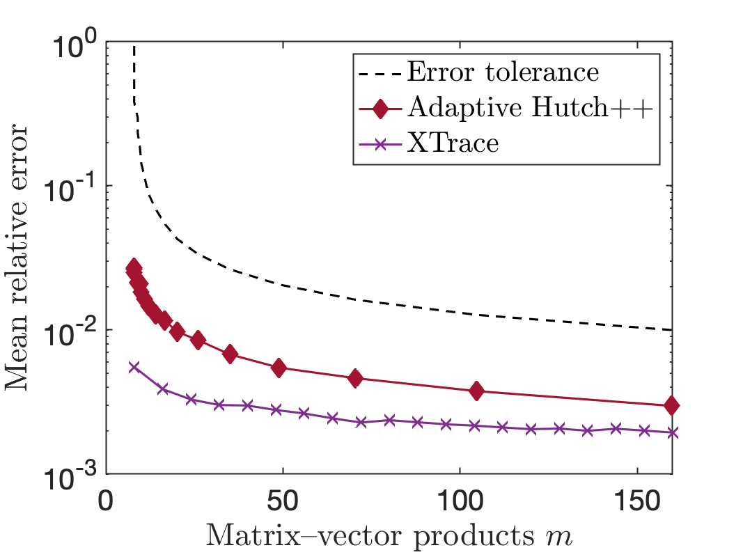
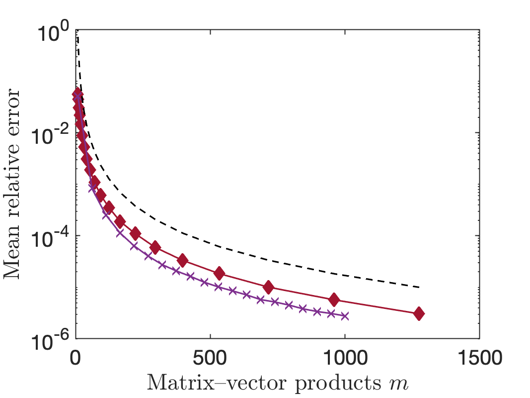
The adaptive Hutch++ algorithm of [28] flexibly apportions test vectors between low-rank approximation and residual trace estimation, based on the estimated singular values of the input matrix. This algorithm interpolates between the Girard–Hutchinson estimator, the Hutch++ estimator, and a purely low-rank approximation-based trace estimate. This algorithm also estimates the total number of matvecs $m$ to meet an (absolute) error tolerance:

$$\left|\widehat{\operatorname{tr}}-\operatorname{tr}(\boldsymbol{A})\right|\leq\varepsilon_{\rm abs}\quad\text{except with probability $1-2\delta$},$$

where $\delta$ is a parameter chosen by the user.

We compare XTrace with adaptive Hutch++ in Fig. SM1. To produce these plots, we first run adaptive Hutch++ with error tolerances $\varepsilon_{\rm abs}=\varepsilon\cdot\operatorname{tr}\boldsymbol{A}$ and failure probability parameter $\delta\coloneqq 1/10$. For each value of the error tolerance $\varepsilon$, we plot the mean error (solid line) and desired accuracy $\varepsilon$ against the mean number $m$ of matvecs required by the algorithm. We then run XTrace with a variable number of matvecs $m$ and report the mean error over $1000$ trials. Overall, we find that XTrace performs similarly to adaptive Hutch++ or better than adaptive Hutch++ by up to an order of magnitude.

(a) flat

(b) poly

(c) exp

(d) step

Figure SM1: Comparison with adaptive Hutch++. Average relative error using XTrace and adaptive Hutch++ (solid lines) and user-chosen error tolerance for Adaptive Hutch++ (dashed lines). See Section SM1.

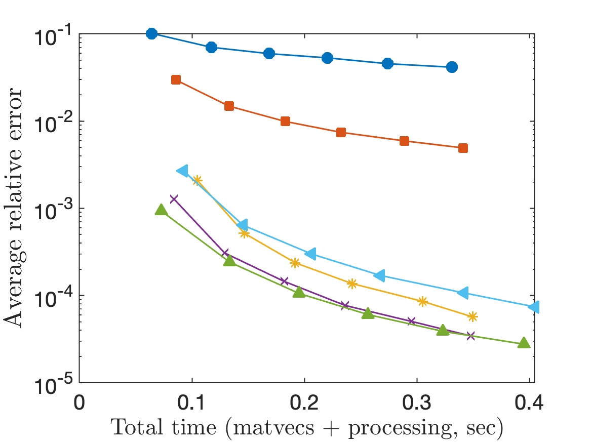
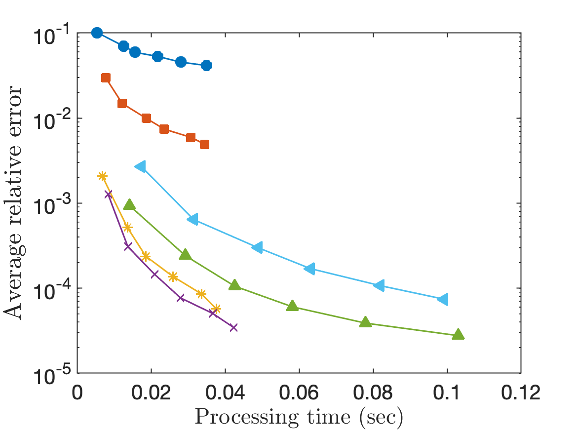
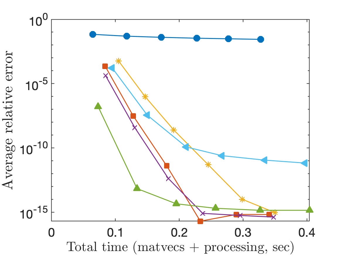
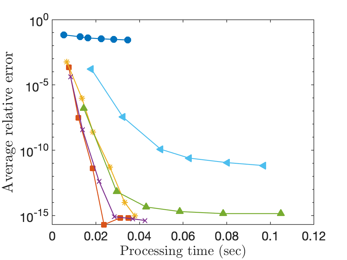
SM2 Runtime comparison

Throughout the main body of the text, we use the number of matrix–vector products as a surrogate for the runtime of different trace estimators, which is justified by the observation that matvecs frequently dominate the cost of trace estimation. For instance, for the quantum statistical physics examples in Sections 1.3.1 and 4.3, matvecs are responsible for over 90% of the runtime for all of the trace estimators. However, when matvec operations are fairly cheap or the number of matvecs is large, the cost of processing the matvecs can come to dominate the runtime.

To illustrate the runtime differences between the algorithms, let us compare the Girard–Hutchinson estimator, Hutch++, and XTrace. The only processing cost of the Girard–Hutchinson algorithm comes from the computation of the inner products $\boldsymbol{\omega}_{i}^{*}(\boldsymbol{A}\boldsymbol{\omega}_{i})$ between the matvecs $\boldsymbol{A}\boldsymbol{\omega}_{i}$ and the test vectors $\boldsymbol{\omega}_{i}$ for $i=1,\ldots,m$, requiring just $\mathcal{O}(mN)$ operations. By contrast, Hutch++ orthogonalizes a matrix of size $N\times(m/3)$, resulting in a higher processing cost of $\mathcal{O}(m^{2}N)$ operations. For a fixed budget of $m$ matvecs, XTrace has the highest processing cost, since the algorithm orthogonalizes a larger $N\times(m/2)$ matrix. Yet, XTrace often compensates for its high processing cost because it results in lower error than the other algorithms.

flat

poly

exp

step

Figure SM2: Runtime. Average relative error versus runtime (left) and processing time (runtime minus matvecs, right); see Section SM2.

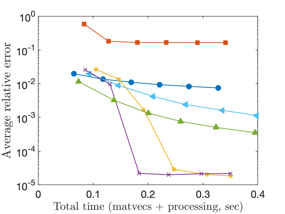
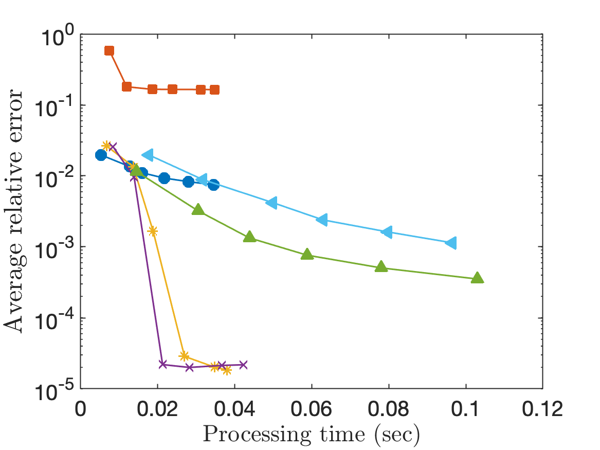
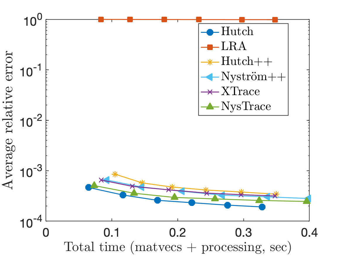
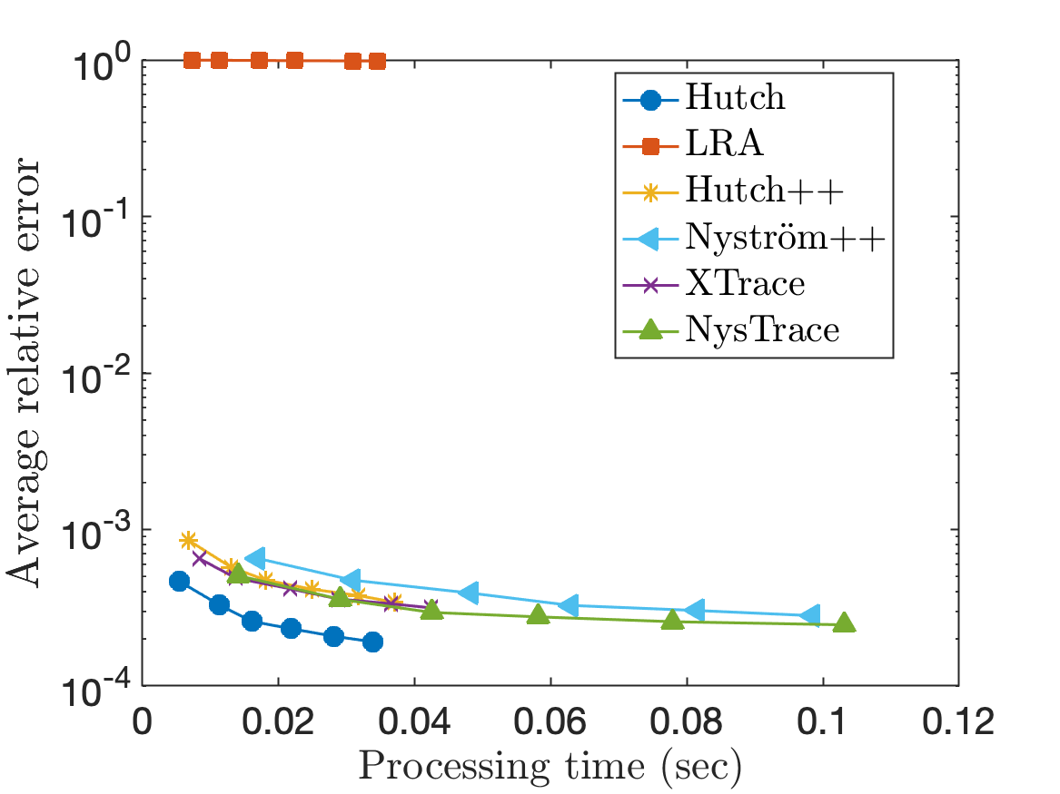
Figure SM2 shows the error versus the runtime for different stochastic trace estimators applied to matrices with several spectral decay patterns. We use the same spectral profiles as in Section 4.1, but use a larger size $N=10^{4}$. In the left panels, we show the error as a function of the total runtime, whereas the right panels show the processing time (total runtime minus the time required to perform the matvecs). Runtimes and errors are computed by averaging over 1000 independent trials.

In these experiments, XTrace consistently achieves lower errors than Hutch++ for a given amount of runtime or processing time, despite the additional costs associated with orthogonalizing a larger matrix. This shows that XTrace can be a more effective trace estimator than Hutch++ even if processing costs begin to dominate the runtime. The processing cost of the Nyström-based trace estimators XNysTrace and Nyström++ is significantly higher than Hutch++ and XTrace. This suggests that when matvecs are expensive, XNysTrace should be preferred over XTrace and when matvecs are cheap, it may be worth using XTrace to avoid XNysTrace’s higher processing costs.

SM3 Derivation for efficient XTrace implementation

In the main text, we proved the update formula

(23) $$\boldsymbol{Q}_{(i)}^{\vphantom{*}}\boldsymbol{Q}_{(i)}^{*}=\boldsymbol{Q}(\mathbf{I}-\boldsymbol{s}_{i}^{\vphantom{*}}\boldsymbol{s}_{i}^{*})\boldsymbol{Q}^{*}$$

for the the $\boldsymbol{Q}_{(i)}$ matrices appearing in the XTrace estimator and devised an $\mathcal{O}(m^{3})$ procedure for computing $\boldsymbol{S}=\begin{bmatrix}\boldsymbol{s}_{1}&\cdots\boldsymbol{s}_{m/2}\end{bmatrix}$. In this section, we complete the derivation of how to compute the basic trace estimators $\widehat{\operatorname{tr}}_{i}$ in $\mathcal{O}(m^{2}N)$ operations.

Instate the notation of Section 2.1. The basic trace estimator $\widehat{\operatorname{tr}}_{i}$ is defined as

$$\widehat{\operatorname{tr}}_{i}=\operatorname{tr}\left(\boldsymbol{Q}_{(i)}^{*}\left(\boldsymbol{A}\boldsymbol{Q}^{\vphantom{*}}_{(i)}\right)\right)+\boldsymbol{\omega}_{i}^{*}\left(\mathbf{I}-\boldsymbol{Q}_{(i)}^{\vphantom{*}}\boldsymbol{Q}_{(i)}^{*}\right)\boldsymbol{A}\left(\mathbf{I}-\boldsymbol{Q}_{(i)}^{\vphantom{*}}\boldsymbol{Q}_{(i)}^{*}\right)\boldsymbol{\omega}_{i}^{\vphantom{*}}$$

Now invoke Eq. 23:

$$\widehat{\operatorname{tr}}_{i}=\operatorname{tr}\left(\boldsymbol{A}\boldsymbol{Q}(\mathbf{I}-\boldsymbol{s}_{i}^{\vphantom{*}}\boldsymbol{s}_{i}^{*})\boldsymbol{Q}^{*}\right)+\boldsymbol{\omega}_{i}^{*}\left(\mathbf{I}-\boldsymbol{Q}(\mathbf{I}-\boldsymbol{s}_{i}^{\vphantom{*}}\boldsymbol{s}_{i}^{*})\boldsymbol{Q}^{*}\right)\boldsymbol{A}\left(\mathbf{I}-\boldsymbol{Q}(\mathbf{I}-\boldsymbol{s}_{i}^{\vphantom{*}}\boldsymbol{s}_{i}^{*})\boldsymbol{Q}^{*}\right)\boldsymbol{\omega}_{i}^{\vphantom{*}}.$$

Define

(24) $$\boldsymbol{Z}\coloneqq\boldsymbol{A}\boldsymbol{Q},\quad\boldsymbol{H}\coloneqq\boldsymbol{Q}^{*}\boldsymbol{Z},\quad\boldsymbol{W}\coloneqq\boldsymbol{Q}^{*}\boldsymbol{\Omega},\quad\boldsymbol{T}\coloneqq\boldsymbol{Z}^{*}\boldsymbol{\Omega},$$

all of which can be computed using $m/2$ matvecs and $\mathcal{O}(m^{2}N)$ operations. Denote the columns of a matrix using the corresponding lowercase letter, e.g., the $i$th column of $\boldsymbol{W}$ is $\boldsymbol{w}_{i}$. Using the newly introduced variables, the trace estimates become

$$\widehat{\operatorname{tr}}_{i} =\operatorname{tr}(\boldsymbol{H})-\boldsymbol{s}_{i}^{*}\boldsymbol{H}\boldsymbol{s}_{i}^{\vphantom{*}}+\boldsymbol{\omega}_{i}^{*}(\mathbf{I}-\boldsymbol{Q}\boldsymbol{Q}^{*})\boldsymbol{A}\boldsymbol{\omega}_{i}+\boldsymbol{w}_{i}^{*}\boldsymbol{s}_{i}^{\vphantom{*}}\boldsymbol{s}_{i}^{*}\boldsymbol{Q}^{*}\boldsymbol{A}\boldsymbol{\omega}_{i}^{\vphantom{*}}$$

$$\qquad-\left(\boldsymbol{\omega}_{i}^{*}-\boldsymbol{w}_{i}^{*}(\mathbf{I}-\boldsymbol{s}_{i}^{\vphantom{*}}\boldsymbol{s}_{i}^{*})\boldsymbol{Q}^{*}\right)\boldsymbol{Z}(\mathbf{I}-\boldsymbol{s}_{i}^{\vphantom{*}}\boldsymbol{s}_{i}^{*})\boldsymbol{w}_{i}^{\vphantom{*}}.$$

To simplify this, we make two observations. First, $\boldsymbol{Q}\boldsymbol{Q}^{*}$ is an orthoprojector onto the range of $\boldsymbol{A}\boldsymbol{\Omega}$, so $(\mathbf{I}-\boldsymbol{Q}\boldsymbol{Q}^{*})\boldsymbol{A}\boldsymbol{\omega}_{i}=\boldsymbol{0}$. Second, recall that we defined and factorized $\boldsymbol{Y}=\boldsymbol{A}\boldsymbol{\Omega}=\boldsymbol{Q}\boldsymbol{R}$. Thus, $\boldsymbol{Q}^{*}\boldsymbol{A}\boldsymbol{\omega}_{i}=\boldsymbol{Q}^{*}\boldsymbol{y}_{i}=\boldsymbol{r}_{i}$. Adding these simplifications, we have

$$\widehat{\operatorname{tr}}_{i} =\operatorname{tr}(\boldsymbol{H})-\boldsymbol{s}_{i}^{*}\boldsymbol{H}\boldsymbol{s}_{i}^{\vphantom{*}}+\boldsymbol{w}_{i}^{*}\boldsymbol{s}_{i}^{\vphantom{*}}\cdot\boldsymbol{s}_{i}^{*}\boldsymbol{r}_{i}^{\vphantom{*}}-\left(\boldsymbol{\omega}_{i}^{*}-\boldsymbol{w}_{i}^{*}(\mathbf{I}-\boldsymbol{s}_{i}^{\vphantom{*}}\boldsymbol{s}_{i}^{*})\boldsymbol{Q}^{*}\right)\boldsymbol{Z}(\mathbf{I}-\boldsymbol{s}_{i}^{\vphantom{*}}\boldsymbol{s}_{i}^{*})\boldsymbol{w}_{i}^{\vphantom{*}}.$$

Now, define

$$\boldsymbol{x}_{i}^{\vphantom{*}}\coloneqq(\mathbf{I}-\boldsymbol{s}_{i}^{\vphantom{*}}\boldsymbol{s}_{i}^{*})\boldsymbol{w}_{i}^{\vphantom{*}}=\boldsymbol{w}_{i}^{\vphantom{*}}-\boldsymbol{s}_{i}^{*}\boldsymbol{w}_{i}^{\vphantom{*}}\cdot\boldsymbol{s}_{i}\quad\text{for $i=1,2,\ldots,m/2$}.$$

Using the new $\boldsymbol{x}_{i}$ notation and the definitions Eq. 24, we conclude

(25) $$\widehat{\operatorname{tr}}_{i}=\operatorname{tr}(\boldsymbol{H})-\boldsymbol{s}_{i}^{*}\boldsymbol{H}\boldsymbol{s}_{i}^{\vphantom{*}}+\boldsymbol{w}_{i}^{*}\boldsymbol{s}_{i}^{\vphantom{*}}\cdot\boldsymbol{s}_{i}^{*}\boldsymbol{r}_{i}^{\vphantom{*}}-\boldsymbol{t}_{i}^{*}\boldsymbol{x}_{i}^{\vphantom{*}}+\boldsymbol{x}_{i}^{*}\boldsymbol{H}\boldsymbol{x}_{i}^{\vphantom{*}}.$$

The update formula Eq. 25 is used to implement XTrace in $\mathcal{O}(m^{2}N)$ operations in Algorithm 4. Algorithm 4 is essentially identical to the MATLAB implementation provided in LABEL:list:xtrace, except that LABEL:list:xtrace uses normalized spherically symmetric test vectors (see Section 2.3) and uses vectorized operations rather than a for loop to compute the basic estimators $\widehat{\operatorname{tr}}_{i}$.

Algorithm 4 XTrace: Efficient implementation

1:Matrix $\boldsymbol{A}\in{}^{N\times N}$ and number $m$ of matvecs, where $m$ is even

2:Trace estimate $\widehat{\operatorname{tr}}\approx\operatorname{tr}\boldsymbol{A}$ and error estimate $\widehat{\mathrm{err}}\approx|\widehat{\operatorname{tr}}-\operatorname{tr}\boldsymbol{A}|$

3:Draw $\boldsymbol{\Omega}\sim\operatorname{\textsc{Unif}}\{\pm 1\}^{N\times m/2}$

4:$\boldsymbol{Y}\leftarrow\boldsymbol{A}\boldsymbol{\Omega}$ $\triangleright$ $m/2$ matvecs

5:$(\boldsymbol{Q},\boldsymbol{R})\leftarrow\mathtt{qr}(\boldsymbol{Y},\texttt{'econ'})$ $\triangleright$ $\mathcal{O}(m^{2}N)$ operations

6:$\boldsymbol{Z}\leftarrow\boldsymbol{A}\boldsymbol{Q}$ $\triangleright$ $m/2$ matvecs

7:$\boldsymbol{H}\leftarrow\boldsymbol{Q}^{*}\boldsymbol{Z}$, $\boldsymbol{W}\leftarrow\boldsymbol{Q}^{*}\boldsymbol{\Omega}$, $\boldsymbol{T}\leftarrow\boldsymbol{Z}^{*}\boldsymbol{\Omega}$ $\triangleright$ $\mathcal{O}(m^{2}N)$ operations

8:$\boldsymbol{S}\leftarrow(\boldsymbol{R}^{*})^{-1}$ $\triangleright$ $\mathcal{O}(m^{3})$ operations

9:$\boldsymbol{S}\leftarrow\boldsymbol{S}\cdot\operatorname{diag}(\left\|\boldsymbol{s}_{i}\right\|^{-1}:i=1,\ldots,m/2)$ $\triangleright$ $\mathcal{O}(m^{2})$ operations

10:for $i=1,\ldots,m/2$ do

11:     $\boldsymbol{x}_{i}\leftarrow\boldsymbol{w}_{i}-\boldsymbol{s}_{i}^{*}\boldsymbol{w}_{i}\cdot\boldsymbol{s}_{i}$ $\triangleright$ $\mathcal{O}(m)$ operations

12:     $\widehat{\operatorname{tr}}_{i}\leftarrow\operatorname{tr}(\boldsymbol{H})-\boldsymbol{s}_{i}^{*}(\boldsymbol{H}\boldsymbol{s}_{i}^{\vphantom{*}})+\boldsymbol{w}_{i}^{*}\boldsymbol{s}_{i}^{\vphantom{*}}\cdot\boldsymbol{s}_{i}^{*}\boldsymbol{r}_{i}^{\vphantom{*}}-\boldsymbol{t}_{i}^{*}\boldsymbol{x}_{i}^{\vphantom{*}}+\boldsymbol{x}_{i}^{*}(\boldsymbol{H}\boldsymbol{x}_{i}^{\vphantom{*}})$ $\triangleright$ $\mathcal{O}(m^{2})$ operations

13:end for

14:$\widehat{\operatorname{tr}}\leftarrow(m/2)^{-1}\sum_{i=1}^{m}\widehat{\operatorname{tr}}_{i}$

15:$\widehat{\mathrm{err}}^{2}\leftarrow((m/2)(m/2-1))^{-1}\sum_{i=1}^{m/2}(\widehat{\operatorname{tr}}_{i}-\widehat{\operatorname{tr}})^{2}$

The derivation of an $\mathcal{O}(m^{2}N)$ implementation for XNysTrace (shown in LABEL:list:xnystrace) is similar in spirit to the one just provided for XTrace and is omitted.

SM4 MATLAB implementations

We present optimized MATLAB R2022b implementations of XTrace, XNysTrace,​ and XDiag in LABEL:list:xtrace, LABEL:list:xnystrace, and LABEL:list:xdiag.

⬇

function [t,err] = xtrace(A, m)

N = size(A,1); m = floor(m/2);

%% Helper functions

cnormc = @(M) M ./ vecnorm(M,2,1);

diag_prod = @(A,B) sum(conj(A).*B,1).’; % computes diag(A’*B)

%% Randomized SVD

Om = sqrt(N)*cnormc(randn(N, m));

Y = A*Om;

[Q,R] = qr(Y,0);

%% Normalization

W = Q’*Om;

S = cnormc(inv(R)’);

scale = (N - m + 1) ./ (N - (vecnorm(W)’).^2 ...

+ abs(diag_prod(S,W) .* vecnorm(S)’).^2);

%% Quantities needed for trace estimation

Z = A*Q; H = Q’*Z; HW = H*W; T=Z’*Om;

dSW = diag_prod(S, W); dSHS = diag_prod(S, H*S);

dTW = diag_prod(T, W); dWHW = diag_prod(W, HW);

dSRmHW = diag_prod(S, R-HW); dTmHRS = diag_prod(T-H’*W,S);

%% Trace estimate

ests = trace(H)*ones(m,1) - dSHS + (dWHW - dTW + dTmHRS .* dSW...

+ abs(dSW).^2 .* dSHS + conj(dSW) .* dSRmHW) .* scale;

t = mean(ests);

err = std(ests)/sqrt(m);

end

Program SM4.1: MATLAB 2022b implementation for XTrace

⬇

function [t,err] = xnystrace(A, m)

N = size(A,1);

%% Helper functions

cnormc = @(M) M ./ vecnorm(M,2,1);

diag_prod = @(A,B) sum(conj(A).*B,1).’; % computes diag(A’*B)

%% Nystrom

Om = sqrt(N) * cnormc(randn(N,m));

Y = A*Om;

nu = eps*norm(Y,’fro’)/sqrt(N);

Y = Y + nu*Om; % Shift for numerical stability

[Q,R] = qr(Y,0);

H = Om’*Y; C = chol((H+H’)/2);

B = R/C; % Nystrom approx is Q*B*B’*Q’

%% Normalization

[QQ,RR] = qr(Om,0);

WW = QQ’*Om;

SS = cnormc(inv(RR)’);

scale = (N - m + 1) ./ (N - vecnorm(WW).^2 ...

+ abs(diag_prod(SS,WW)’ .* vecnorm(SS)).^2);

%% Trace estimate

W = Q’*Om; S = (B/C’) .* (diag(inv(H))’).^(-0.5);

dSW = diag_prod(S, W).’;

ests = norm(B,’fro’)^2 - vecnorm(S).^2 + abs(dSW).^2 .* scale...

- nu*N;

t = mean(ests);

err = std(ests)/sqrt(m);

end

Program SM4.2: MATLAB 2022b implementation for XNysTrace

⬇

function d = xdiag(A, m)

N = size(A,1); m = floor(m/2);

%% Helper functions

cnormc = @(M) M ./ vecnorm(M,2,1);

diag_prod = @(A,B) sum(conj(A).*B,1).’; % computes diag(A’*B)

%% Randomized SVD

Om = -3 + 2*randi(2,n,m); % Random signs

Y = A*Om;

[Q,R] = qr(Y,0);

% Quantities needed for trace estimation

Z = A’*Q; T=Z’*Om;

S = cnormc(inv(R)’);

dQZ = diag_prod(Q’,Z’); dQSSZ = diag_prod((Q*S)’,(Z*S)’);

dOmQT = diag_prod(Om’,(Q*T).’); dOmY = diag_prod(Om’,Y.’);

dOmQSST = diag_prod(Om’,(Q*S*diag(diag_prod(S,T))).’);

% Trace estimate

d = dQZ + (-dQSSZ+dOmY-dOmQT+dOmQSST)/m;

end

Program SM4.3: MATLAB 2022b implementation for XDiag

References

• [1] M. Al Hasan and V. S. Dave, Triangle counting in large networks: A review, WIREs Data Mining and Knowledge Discovery, 8 (2018), p. e1226, https://doi.org/10.1002/widm.1226.
• [2] A. H. Al-Mohy and N. J. Higham, Computing the action of the matrix exponential, with an application to exponential integrators, SIAM Journal on Scientific Computing, 33 (2011), pp. 488–511, https://doi.org/10.1137/100788860.
• [3] H. Avron, P. Maymounkov, and S. Toledo, Blendenpik: Supercharging LAPACK’s least-squares solver, SIAM Journal on Scientific Computing, 32 (2010), pp. 1217–1236, https://doi.org/10.1137/090767911.
• [4] R. A. Baston and Y. Nakatsukasa, Stochastic diagonal estimation: Probabilistic bounds and an improved algorithm, Jan. 2022, https://arxiv.org/abs/2201.10684v1.
• [5] C. Bekas, E. Kokiopoulou, and Y. Saad, An estimator for the diagonal of a matrix, Applied Numerical Mathematics, 57 (2007), pp. 1214–1229, https://doi.org/10.1016/j.apnum.2007.01.003.
• [6] D. Bu, Y. Zhao, L. Cai, H. Xue, X. Zhu, H. Lu, J. Zhang, S. Sun, L. Ling, N. Zhang, G. Li, and R. Chen, Topological structure analysis of the protein–protein interaction network in budding yeast, Nucleic Acids Research, 31 (2003), pp. 2443–2450, https://doi.org/10.1093/nar/gkg340.
• [7] T. Chen and E. Hallman, Krylov-aware stochastic trace estimation, Nov. 2022, https://arxiv.org/abs/2205.01736v2.
• [8] T. Chen, T. Trogdon, and S. Ubaru, Randomized matrix-free quadrature for spectrum and spectral sum approximation, Sept. 2022, https://arxiv.org/abs/2204.01941v2.
• [9] T. Davis and Y. Hu, The University of Florida sparse matrix collection, ACM Transactions on Mathematical Software, 38 (2011), pp. 1–25, https://doi.org/10.1145/2049662.2049663.
• [10] E. N. Epperly and J. A. Tropp, Efficient error and variance estimation for randomized matrix computations, Mar. 2023, https://arxiv.org/abs/2207.06342v3.
• [11] E. Estrada, The many facets of the Estrada indices of graphs and networks, SeMA Journal, 79 (2022), pp. 57–125, https://doi.org/10.1007/s40324-021-00275-w.
• [12] A. S. Gambhir, A. Stathopoulos, and K. Orginos, Deflation as a method of variance reduction for estimating the trace of a matrix inverse, SIAM Journal on Scientific Computing, 39 (2017), pp. A532–A558, https://doi.org/10.1137/16M1066361.
• [13] A. C. Gilbert, M. J. Strauss, J. A. Tropp, and R. Vershynin, One sketch for all: Fast algorithms for compressed sensing, in Proceedings of the Thirty-Ninth Annual ACM Symposium on Theory of Computing, June 2007, pp. 237–246, https://doi.org/10.1145/1250790.1250824.
• [14] A. Girard, A fast“Monte-Carlo cross-validation” procedure for large least squares problems with noisy data, Numerische Mathematik, 56 (1989), pp. 1–23, https://doi.org/10.1007/BF01395775.
• [15] N. Halko, P.-G. Martinsson, and J. A. Tropp, Finding structure with randomness: Probabilistic algorithms for constructing approximate matrix decompositions, SIAM Review, 53 (2011), pp. 217–288, https://doi.org/10.1137/090771806.
• [16] P. R. Halmos, The theory of unbiased estimation, The Annals of Mathematical Statistics, 17 (1946), pp. 34–43, https://doi.org/10.1214/aoms/1177731020.
• [17] N. J. Higham, Functions of Matrices: Theory and Computation, SIAM, Philadelphia, 2008, https://doi.org/10.1137/1.9780898717778.
• [18] N. J. Higham, Matrix exponential times a vector, Nov. 2010. Available at https://www.mathworks.com/matlabcentral/fileexchange/29576-matrix-exponential-times-a-vector (accessed 10/25/2022).
• [19] M. F. Hutchinson, A stochastic estimator of the trace of the influence matrix for Laplacian smoothing splines, Communications in Statistics - Simulation and Computation, 18 (1989), pp. 1059–1076, https://doi.org/10.1080/03610918908812806.
• [20] S. Jiang, H. Pham, D. P. Woodruff, and Q. Zhang, Optimal sketching for trace estimation, in 35th Conference on Neural Information Processing Systems., 2021, p. 13.
• [21] V. S. Koroljuk and Y. V. Borovskich, Theory of U-Statistics, Springer Netherlands, Dordrecht, 1994, https://doi.org/10.1007/978-94-017-3515-5.
• [22] H. Li, G. C. Linderman, A. Szlam, K. P. Stanton, Y. Kluger, and M. Tygert, Algorithm 971: An implementation of a randomized algorithm for principal component analysis, ACM Transactions On Mathematical Software, 43 (2017), https://doi.org/10.1145/3004053.
• [23] L. Lin, Randomized estimation of spectral densities of large matrices made accurate, Numerische Mathematik, 136 (2017), pp. 183–213, https://doi.org/10.1007/s00211-016-0837-7.
• [24] C. Litens, Transverse Field Ising Model with Different Boundary Conditions, Bachelor’s Thesis, Stockholm University, Feb. 2019. Available at http://staff.fysik.su.se/~ardonne/files/theses/bachelor-thesis_christopher-litens.pdf.
• [25] P.-G. Martinsson and J. A. Tropp, Randomized numerical linear algebra: Foundations and algorithms, Acta Numerica, 29 (2020), pp. 403–572, https://doi.org/10.1017/S0962492920000021.
• [26] R. A. Meyer, C. Musco, C. Musco, and D. P. Woodruff, Hutch++: Optimal stochastic trace estimation, in Symposium on Simplicity in Algorithms, SIAM, Jan. 2021.
• [27] R. A. Meyer, C. Musco, C. Musco, and D. P. Woodruff, Hutch++: Optimal stochastic trace estimation, June 2021, https://arxiv.org/abs/2002.11457v5.
• [28] D. Persson, A. Cortinovis, and D. Kressner, Improved variants of the Hutch++ algorithm for trace estimation, SIAM Journal on Matrix Analysis and Applications, (2022), pp. 1162–1185, https://doi.org/10.1137/21M1447623.
• [29] P. Pfeuty, The one-dimensional Ising model with a transverse field, Annals of Physics, 57 (1970), pp. 79–90, https://doi.org/10.1016/0003-4916(70)90270-8.
• [30] V. Rokhlin and M. Tygert, A fast randomized algorithm for overdetermined linear least-squares regression, Proceedings of the National Academy of Sciences, 105 (2008), pp. 13212–13217, https://doi.org/10.1073/pnas.0804869105.
• [31] A. K. Saibaba, A. Alexanderian, and I. C. F. Ipsen, Randomized matrix-free trace and log-determinant estimators, Numerische Mathematik, 137 (2017), pp. 353–395, https://doi.org/10.1007/s00211-017-0880-z.
• [32] J. A. Tropp and R. J. Webber, Randomized algorithms for low-rank matrix approximation: Design, analysis, and applications, June 2023, https://doi.org/10.48550/arXiv.2306.12418v1.
• [33] J. A. Tropp, A. Yurtsever, M. Udell, and V. Cevher, Fixed-rank approximation of a positive-semidefinite matrix from streaming data, in Advances in Neural Information Processing Systems, vol. 30, 2017, pp. 1225–1234.
• [34] S. Ubaru, J. Chen, and Y. Saad, Fast estimation of $\operatorname{tr}(f({{A}}))$ via stochastic Lanczos quadrature, SIAM Journal on Matrix Analysis and Applications, 38 (2017), pp. 1075–1099, https://doi.org/10.1137/16M1104974.
• [35] S. Ubaru and Y. Saad, Applications of trace estimation techniques, in High Performance Computing in Science and Engineering, 2017, https://doi.org/10.1007/978-3-319-97136-0_2.