Sample-Efficient Multi-Objective Learning via
Generalized Policy Improvement Prioritization

Abstract.

Multi-objective reinforcement learning (MORL) algorithms tackle sequential decision problems where agents may have different preferences over (possibly conflicting) reward functions. Such algorithms often learn a set of policies (each optimized for a particular agent preference) that can later be used to solve problems with novel preferences. We introduce a novel algorithm that uses Generalized Policy Improvement (GPI) to define principled, formally-derived prioritization schemes that improve sample-efficient learning. They implement active-learning strategies by which the agent can (i) identify the most promising preferences/objectives to train on at each moment, to more rapidly solve a given MORL problem; and (ii) identify which previous experiences are most relevant when learning a policy for a particular agent preference, via a novel Dyna-style MORL method. We prove our algorithm is guaranteed to always converge to an optimal solution in a finite number of steps, or an $\epsilon$-optimal solution (for a bounded $\epsilon$) if the agent is limited and can only identify possibly sub-optimal policies. We also prove that our method monotonically improves the quality of its partial solutions while learning. Finally, we introduce a bound that characterizes the maximum utility loss (with respect to the optimal solution) incurred by the partial solutions computed by our method throughout learning. We empirically show that our method outperforms state-of-the-art MORL algorithms in challenging multi-objective tasks, both with discrete and continuous state and action spaces.

1. Introduction

Reinforcement learning (RL) algorithms Sutton and Barto (2018) have achieved remarkable successes in a wide range of complex tasks (e.g., Silver et al. (2017); Bellemare et al. (2020); Wurman et al. (2022)). In RL, tasks are typically modeled via a single scalar reward function, which encodes the agent’s objective. In many real-life settings, by contrast, agents are tasked with optimizing behaviors that trade-off between multiple—possibly conflicting—objectives, each of which is modeled via a reward function. As an example, consider a robot that needs to trade off between locomotion speed, battery usage, and accuracy in reaching a goal location. Multi-Objective RL (MORL) Hayes et al. (2022) algorithms tackle such a challenge. In MORL settings, a utility function exists that combines (into a single scalar value) the agent’s preferences toward optimizing each of its objectives. The goal of MORL algorithms is to rapidly identify policies that maximize the utility function, given any preferences an agent may have.

Standard RL algorithms are often sample-inefficient since they may require the agent to interact with its environment a large number of times Sutton and Barto (2018). This is often infeasible, e.g., in applications where interactions are costly or risky. The sample efficiency problem is exacerbated in MORL algorithms, since they often have to learn not a single policy, but a set of policies—each designed to optimize a particular trade-off between the agent’s preferences Yang et al. (2019).

In this paper, we introduce a novel MORL algorithm, with important theoretical guarantees, that improves sample efficiency via two novel prioritization techniques. Such principled techniques allow the agent to (i) identify the most promising preferences/objectives to train on at each moment, to more rapidly solve a MORL problem; and (ii) identify which previous experiences are most relevant when learning a policy for a particular agent preference, via a novel Dyna-style MORL method. We show formal analyses and proofs regarding our algorithm’s convergence properties, as well as the maximum utility loss (performance) incurred by the transient solutions computed by our method throughout the learning process.

To design a method with these properties, we exploit an important concept in the RL literature: Generalized Policy Improvement (GPI) Barreto et al. (2020). GPI is a policy transfer technique that—given a set of policies—constructs a novel policy guaranteed to be at least as good as any of the available ones. First, recall that if the utility function of a MORL problem is a linear combination of the agent’s objectives, optimal solutions are sets of policies known as convex coverage sets (CCS) Roijers et al. (2013). Given a CCS, agents can directly identify the optimal solution to any novel preferences. MORL algorithms that learn a CCS (e.g., Alegre et al. (2022a); Mossalam et al. (2016)) may be sample inefficient (i) due to the heuristics they use to determine which preferences to train on, at any given moment during the construction of a CCS; and (ii) because they can only improve a CCS after optimal (or near-optimal) policies are identified—which may require a large number of samples. We address the first issue via a novel GPI-based prioritization technique for selecting which preferences to train on. It is based on a lower bound on performance improvements that are formally guaranteed to be achievable, and more accurately and reliably identifies the most relevant preferences to train on (when constructing a CCS) compared to existing heuristics. To address the second issue, we show that our method is an anytime algorithm that incrementally/monotonically improves the quality of its CCS, even if given intermediate (possibly sub-optimal) policies for different preferences. This improves sample efficiency: our method identifies intermediate CCSs with formally bounded maximum utility loss even if there are constraints on the number of times the agent can interact with its environment. Our algorithm is guaranteed to always converge to an optimal solution in a finite number of steps, or an $\epsilon$-optimal solution (for a bounded $\epsilon$) if the agent is limited and can only identify possibly sub-optimal policies. We prove that it monotonically improves the quality of its CCS and formally bound the maximum utility loss (with respect to an optimal solution) incurred by any of its partial solutions.

A complementary approach for increasing sample efficiency is to use a model-based approach to learn policies for different preferences. Once a model is learned, it can be used to identify policies for any preferences, thus minimizing the required number of interactions with the environment. We introduce a novel Dyna-style MORL algorithm—the first model-based MORL technique capable of dealing with continuous state spaces. Dyna algorithms are based on generating simulated experiences to more rapidly update a value function or policy. An important question, however, is which artificial experiences should be generated to accelerate learning. We introduce a new, principled GPI-based prioritization technique for identifying which experiences are most relevant to rapidly learn the optimal policy for novel preferences.

In summary, we introduce two novel GPI-based prioritization techniques for use in MORL settings to improve sample efficiency. We formally show that our algorithm is supported by important theorems characterizing its convergence properties and performance bounds. We empirically show that our method outperforms state-of-the-art MORL algorithms in challenging multi-objective tasks, both with discrete and continuous state and action spaces.

2. Background

In this section, we discuss important definitions (and corresponding notation) associated with MORL, GPI, and model-based RL.

2.1. Multi-Objective Reinforcement Learning

The multi-objective RL setting (MORL) is used to model problems where an agent needs to optimize possibly conflicting objectives, each modeled via a separate reward function. MORL problems are modeled as Multi-objective Markov decision processes (MOMDP), which differ from regular MDPs in that the reward function is vector-valued. A MOMDP is defined as a tuple $M\equiv(\mathcal{S},\mathcal{A},p,\bm{\mathbf{r}},\mu,\gamma)$, where $\mathcal{S}$ is a state space, $\mathcal{A}$ is an action space, $p(\cdot|s,a)$ is the distribution over next states given state $s$ and action $a$, $\bm{\mathbf{r}}:\mathcal{S}{\times}\mathcal{A}{\times}\mathcal{S}{\mapsto}\mathbb{R}^{m}$ is a multi-objective reward function with $m$ objectives, $\mu$ is an initial state distribution, and $\gamma\in[0,1)$ is a discounting factor. Let $S_{t}$, $A_{t}$, and $\bm{\mathbf{R}}_{t}=\bm{\mathbf{r}}(S_{t},A_{t},S_{t+1})$ be random variables corresponding to the state, action, and vector reward, respectively, at time step $t$. A policy $\pi:\mathcal{S}\mapsto\mathcal{A}$ is a function mapping states to actions. The multi-objective action-value function of a policy $\pi$ for a given state-action pair $(s,a)$ is defined as:

$$\bm{\mathbf{q}}^{\pi}(s,a)\equiv\mathbb{E}_{\pi}\left[\sum_{i=0}^{\infty}\gamma^{i}\bm{\mathbf{R}}_{t+i}\ |\ S_{t}=s,A_{t}=a\right],$$ (1)

where $\bm{\mathbf{q}}^{\pi}(s,a)$ is an $m$-dimensional vector whose $i$-th entry is the expect return of $\pi$ under the $i$-th objective, and $\mathbb{E}_{\pi}[\cdot]$ denotes expectation over trajectories induced by $\pi$. Let $\bm{\mathbf{v}}^{\pi}{\in}\mathbb{R}^{m}$ be the multi-objective value vector of $\pi$ under the initial state distribution $\mu$:

$$\bm{\mathbf{v}}^{\pi}\equiv\mathbb{E}_{S_{0}\sim\mu}\left[\bm{\mathbf{q}}^{\pi}(S_{0},\pi(S_{0}))\right],$$ (2)

where $v^{\pi}_{i}$ is the value of $\pi$ under the $i$-th objective. For succinctness, we henceforth refer to $\bm{\mathbf{v}}^{\pi}$ as the value vector of policy $\pi$. A Pareto frontier is a set of nondominated multi-objective value functions $\bm{\mathbf{v}}^{\pi}$: $\mathcal{F}\equiv\{\bm{\mathbf{v}}^{\pi}\ |\ \nexists\ \pi^{\prime}\mathrm{s.t.}\ \bm{\mathbf{v}}^{\pi^{\prime}}\succ_{p}\bm{\mathbf{v}}^{\pi}\},$ where $\succ_{p}$ is the Pareto dominance relation $\bm{\mathbf{v}}^{\pi}\succ_{p}\bm{\mathbf{v}}^{\pi^{\prime}}\iff(\forall i:v^{\pi}_{i}\geq v^{\pi^{\prime}}_{i})\land(\exists i:v^{\pi}_{i}>v^{\pi^{\prime}}_{i})$. In general, the optimal solution to a MOMDP is a set of all policies $\pi$ such that $\bm{\mathbf{v}}^{\pi}$ is in the Pareto frontier.

Let a user utility function (or scalarization function) $u:\mathbb{R}^{m}\mapsto\mathbb{R}$ be a mapping from the multi-objective value of policy $\pi$, $\bm{\mathbf{v}}^{\pi}$, to a scalar. Utility functions often linearly combine the value of a policy under each of the $m$ objectives using a set of weights $\bm{\mathbf{w}}$: $u(\bm{\mathbf{v}}^{\pi},\bm{\mathbf{w}})=v_{\bm{\mathbf{w}}}^{\pi}=\bm{\mathbf{v}}^{\pi}\cdot\bm{\mathbf{w}},$ where each element of $\bm{\mathbf{w}}\in\mathbb{R}^{m}$ specifies the relative importance of each objective. The space of weight vectors, $\mathcal{W}$, is an $m$-dimensional simplex: $\textstyle\sum_{i}w_{i}=1,w_{i}\geq 0,i=1,...,m$. For any given constant $\bm{\mathbf{w}}$ (i.e., a particular way of weighting objectives), the original MOMDP collapses into an MDP with reward function $r_{\bm{\mathbf{w}}}(s,a,s^{\prime})=\bm{\mathbf{r}}(s,a,s^{\prime})\cdot\bm{\mathbf{w}}$. Given a linear utility function $u$, we can define a convex coverage set (CCS) Roijers et al. (2013) as a finite convex subset of $\mathcal{F}$, such that there exists a policy in the set that is optimal with respect to any linear preference $\bm{\mathbf{w}}$. In other words, the CCS is the set of nondominated multi-objective value functions $\bm{\mathbf{v}}^{\pi}$ where the dominance relation is now defined over scalarized values:

$$\mathrm{CCS}\equiv\{\bm{\mathbf{v}}^{\pi}\in\mathcal{F}\ |\ \exists\bm{\mathbf{w}}\ \text{s.t.}\ \forall\bm{\mathbf{v}}^{\pi^{\prime}}\in\mathcal{F},\bm{\mathbf{v}}^{\pi}\cdot\bm{\mathbf{w}}\geq\bm{\mathbf{v}}^{\pi^{\prime}}\cdot\bm{\mathbf{w}}\},$$ (3)

where $\bm{\mathbf{w}}$ is a vector of weights used by the scalarization function $u$. Hence, the optimal solution to a MOMDP, under linear preferences, is a finite convex subset of the Pareto frontier.

2.2. Generalized Policy Improvement

Generalized Policy Improvement (GPI) is a generalization of the policy improvement step Puterman (2005), which underlies most of the RL algorithms. The key difference is that GPI defines a new policy that improves over a set of policies, instead of a single one. GPI was originally proposed to be employed in the setting where policies are evaluated using their successor features Barreto et al. (2017, 2020). However, Alegre et al. Alegre et al. (2022a) showed that GPI can also be employed with multi-objective action-value functions (Eq. (1)).

Let $\Pi=\{\pi_{i}\}_{i=1}^{n}$ be a set of previously-learned policies with corresponding multi-objective action-value functions $\{\bm{\mathbf{q}}^{\pi_{i}}\}_{i=1}^{n}$. Given any weight vector $\bm{\mathbf{w}}{\in}\mathcal{W}$, we can directly evaluate all policies $\pi_{i}\in\Pi$ by computing the dot product of its multi-objective action-values and the weight vector: $q^{\pi_{i}}_{\bm{\mathbf{w}}}(s,a)=\bm{\mathbf{q}}^{\pi_{i}}(s,a)\cdot\bm{\mathbf{w}}$. This step is known as generalized policy evaluation (GPE) Barreto et al. (2020). We define the GPI policy as a policy $\pi:\mathcal{S}\times\mathcal{W}\mapsto\mathcal{A}$ that is constructed from a set of policies $\Pi$, and is conditioned on a weight vector $\bm{\mathbf{w}}\in\mathcal{W}$:

$$\pi^{\text{GPI}}(s;\bm{\mathbf{w}})\in\operatorname*{arg\,max}_{a\in\mathcal{A}}\max_{\pi\in\Pi}q^{\pi}_{\bm{\mathbf{w}}}(s,a).$$ (4)

Let $q^{\text{GPI}}_{\bm{\mathbf{w}}}(s,a)$ be the action-value function of policy $\pi^{\text{GPI}}(\cdot;\bm{\mathbf{w}})$. The GPI theorem Barreto et al. (2017) ensures that $q^{\text{GPI}}_{\bm{\mathbf{w}}}(s,a)\geq\max_{\pi\in\Pi}q_{\bm{\mathbf{w}}}^{\pi}(s,a)$ for all $(s,a)\in\mathcal{S}\times\mathcal{A}$. In other words, GPI allows for the rapid identification of a policy that is guaranteed to perform at least as well as any of the policies $\pi_{i}\in\Pi$, for any given weight vector $\bm{\mathbf{w}}\in\mathcal{W}$. This result is also valid and can be extended to the scenario where $q^{\pi_{i}}$ is replaced with estimates/approximations, $\tilde{Q}^{\pi_{i}}$ Barreto et al. (2018).

2.3. Model-Based RL

In model-based RL Moerland et al. (2020), an agent learns—based on experiences collected while interacting with the environment—an approximate model $\tilde{p}(s^{\prime},r|s,a)$ of the joint distribution over the next states and rewards. This model can be employed in multiple ways, such as: (i) to perform Dyna-style planning, i.e., generate simulated experiences to more rapidly learn a policy or value function Van Seijen and Sutton (2013); Janner et al. (2019); Pan et al. (2019); (ii) produce improved model-augmented update targets for use by temporal-difference algorithms Feinberg et al. (2018); Buckman et al. (2018); Abbas et al. (2020); (iii) to perform planning, online, via Model Predictive Control techniques Chua et al. (2018); and (iv) to exploit model gradients with respect to its parameters to improve the efficiency of policy parameter updates Deisenroth and Rasmussen (2011); D’Oro and Jaskowski (2020).

One widely-used model-based framework is based on the Dyna architecture Sutton (1990), by which an agent learns a model and updates a value function/policy using real and model-generated, simulated experiences. This significantly improves sample efficiency, as demonstrated by recent successes of RL when using expressive function approximators Pan et al. (2018); Janner et al. (2019); Kaiser et al. (2020). The key insight is that performing additional updates, using model-generated experiences, reduces the need to frequently interact with the environment, which may be expensive and risky in real-world applications.

A crucial component of Dyna-style algorithms is the search-control mechanism, which prioritizes and samples (from the learned model) experiences to be used in Dyna planning. The classic Dyna algorithm samples state-action pairs uniformly. Other variants have been studied. For example, the Prioritized Sweeping algorithm Moore and Atkeson (1993) prioritizes states or state-action pairs with higher absolute temporal-difference error (TD-error) $\delta_{t}$ when performing value updates. A similar idea has been extensively investigated in models that are based, e.g., on Prioritized Experience Replay buffers Lin (1992); Schaul et al. (2016); Fujimoto et al. (2020), which are a form of (limited) non-parametric models Van Seijen and Sutton (2015). According to the Prioritized Experience Replay method, the probability of sampling a given state-action pair, $P(s,a)$, is defined by

$$P(S_{t},A_{t})\propto|\delta_{t}|,\quad\delta_{t}=R_{t}+\gamma\max_{a^{\prime}\in\mathcal{A}}q^{\pi}(S_{t+1},a^{\prime})-q^{\pi}(S_{t},A_{t}).$$ (5)

Intuitively, states with higher TD-error are more likely to cause larger changes in post-update value functions, and therefore are also likely to accelerate policy learning.

3. Sample-Efficient MORL

Since our objective is to improve sample efficiency in MORL settings (and given the observations in Section 2.1), we propose to design a method to rapidly learn a set of policies $\Pi$ whose values approximate a CCS (Eq. (3)). In this Section, we first introduce a novel method based on GPI to identify the most promising preferences/weight vectors $\bm{\mathbf{w}}\in\mathcal{W}$ to train on, at each moment, while constructing a CCS (Section 3.1). Then, we introduce a principled technique to prioritize experiences (for use when optimizing a given preference) based on the formally-guaranteed improvements achievable via a one-step GPI process (Section 3.2). These contributions are combined in Section 4 to derive an effective algorithm that approximates the CCS in discrete- and continuous-state settings.

3.1. Prioritizing Weight Vectors via GPI

In this Section, we introduce a principled algorithm that iteratively constructs a set of policies, $\Pi$, whose value vectors, $\mathcal{V}$, approximate the CCS. At each iteration, it selects a weight vector $\bm{\mathbf{w}}\in\mathcal{W}$ based on the formally-guaranteed improvements achievable via GPI, and learns a new policy $\pi_{\bm{\mathbf{w}}}$ specialized in optimizing $\bm{\mathbf{w}}$.

1

Input : MOMDP $M$

2

3$\pi_{\bm{\mathbf{w}}},\bm{\mathbf{v}}^{\pi_{\bm{\mathbf{w}}}}\leftarrow\mathrm{NewPolicy}(\bm{\mathbf{w}}=[1,0,...,0]^{\top})$

4 $\Pi\leftarrow\{\pi_{\bm{\mathbf{w}}}\},\mathcal{V}\leftarrow\{\bm{\mathbf{v}}^{\pi_{\bm{\mathbf{w}}}}\}$, $\mathcal{M}\leftarrow\{\}$

5 while True do

6       $\mathcal{W}_{\mathrm{corner}}\leftarrow\mathrm{CornerWeights(\mathcal{V})}\setminus\mathcal{M}$

7       if $\mathcal{W}_{\mathrm{corner}}$ is empty then

             return $\Pi,\mathcal{V}$;

              $\triangleright$ Found CCS (or $\epsilon$-CCS)

8            

9      $\bm{\mathbf{w}}\leftarrow\operatorname*{arg\,max}_{\bm{\mathbf{w}}\in\mathcal{W}_{\mathrm{corner}}}(v^{\mathrm{GPI}}_{\bm{\mathbf{w}}}-\max_{\pi\in\Pi}v^{\pi}_{\bm{\mathbf{w}}})$

10      

11      $\pi_{\bm{\mathbf{w}}},\bm{\mathbf{v}}^{\pi_{\bm{\mathbf{w}}}},\mathrm{done}\leftarrow\mathrm{NewPolicy}(\bm{\mathbf{w}},\Pi)$

12       if $\mathrm{done}$ then

             Add $\bm{\mathbf{w}}$ to $\mathcal{M}$;

              $\triangleright$ Adds $\bm{\mathbf{w}}$ to support of partial CCS

13            

14      Add $\pi_{\bm{\mathbf{w}}}$ to $\Pi$ and $\bm{\mathbf{v}}^{\pi_{\bm{\mathbf{w}}}}$ to $\mathcal{V}$

15       $\Pi,\mathcal{V}\leftarrow\mathrm{RemoveDominated}(\Pi,\mathcal{V})$

16      

Algorithm 1 GPI Linear Support (GPI-LS)

We start by defining the corner weights Roijers (2016) of a given set of value vectors, $\mathcal{V}$. Corner weights $\mathcal{W}_{\mathrm{corner}}\subset\mathcal{W}$ are a finite subset of the weight vector space with relevant properties we will explore.

Definition .

Let $\mathcal{V}=\{\bm{\mathbf{v}}^{\pi_{i}}\}_{i=1}^{n}$ be a set of multi-objective value functions of $n$ policies. Corner weights are the weights contained in the vertices of a polyhedron, $P$, defined as:

$$P=\{\bm{\mathbf{x}}\in\mathbb{R}^{d+1}\ |\ \bm{\mathbf{V}}^{+}\bm{\mathbf{x}}\leq\bm{\mathbf{0}},\textstyle\sum_{i}w_{i}=1,w_{i}\geq 0,\forall i\},$$ (6)

where $\bm{\mathbf{V}}^{+}$ is a matrix whose rows store the elements of $\mathcal{V}$ and is augmented by a column vector of $-1$’s. Each vector $\bm{\mathbf{x}}{=}(w_{1},...,w_{d},v_{\bm{\mathbf{w}}})$ in $P$ is composed of a weight vector and its scalarized value.

Intuitively, corner weights are the weight vectors for which the policy selected in the maximization $\max_{\pi\in\Pi}v^{\pi}_{\bm{\mathbf{w}}}$ changes. These are weight vectors for which two or more policies in $\Pi$ share the same value with respect to the above-mentioned maximization. Extrema weights (weights where only one element is 1 and all others are 0) are special cases of corner weights. Notice that the number of vertices of the polyhedron $P$ is finite when $\mathcal{V}$ is finite. The importance of corner weights comes from the following theorem: (Theorem 7 of Roijers Roijers (2016)). Let $\Pi=\{\pi_{i}\}_{i=1}^{n}$ be a set of $n$ policies with corresponding value vectors $\mathcal{V}=\{\bm{\mathbf{v}}^{\pi_{i}}\}_{i=1}^{n}$. Let $\Delta(\bm{\mathbf{w}},\Pi)=v^{*}_{\bm{\mathbf{w}}}-\max_{\pi\in\Pi}v^{\pi}_{\bm{\mathbf{w}}}$ be the utility loss of weight vector $\bm{\mathbf{w}}\in\mathcal{W}$ given the policy set $\Pi$; that is, the difference between the value of the optimal policy for $\bm{\mathbf{w}}$ and the value that can be obtained if using one of the policies in $\Pi$ for solving $\bm{\mathbf{w}}$. Then, a weight vector $\bm{\mathbf{w}}\in\arg\max_{\bm{\mathbf{w}}\in\mathcal{W}}\,\,\Delta(\bm{\mathbf{w}},\Pi)$ is one of the corner weights of $\mathcal{V}$. Due to this theorem, when selecting a weight vector to train on when constructing a CCS, we only need to consider the finite set of corner weights, $\mathcal{W}_{\mathrm{corner}}$, instead of the infinite weight simplex $\mathcal{W}$. However, this does tell us how to select a weight vector (among all the corner weights) to more rapidly learn the CCS. Let $v^{\mathrm{GPI}}_{\bm{\mathbf{w}}}$ be the scalarized value of the GPI policy (Eq. 4) for the weight vector $\bm{\mathbf{w}}$. We propose to prioritize weight vectors based on the magnitude of the improvement that can be formally achieved via GPI. In particular, given the corner weights $\mathcal{W}_{\mathrm{corner}}$ of the current value set, $\mathcal{V}$, we select the weight vector $\bm{\mathbf{w}}{\in}\mathcal{W}_{\mathrm{corner}}$ given by:

$$\operatorname*{arg\,max}_{\bm{\mathbf{w}}\in\mathcal{W}_{\mathrm{corner}}}(v^{\mathrm{GPI}}_{\bm{\mathbf{w}}}-\max_{\pi\in\Pi}v^{\pi}_{\bm{\mathbf{w}}}).$$ (7)

Intuitively, Eq. (7) identifies the corner weight for which we are guaranteed to achieve the maximum possible improvement via GPI.

In Alg. 1 we show an iterative algorithm, GPI Linear Support (GPI-LS), that constructs a CCS in a finite number of iterations based on the above-mentioned ideas. Let $\mathrm{NewPolicy}(\bm{\mathbf{w}},\Pi)$ be any RL algorithm that searches for a policy that optimizes a weight vector $w{\in}\mathcal{W}$, starting from an initial candidate policy $\pi_{\bm{\mathbf{w}}}$ set to $\operatorname*{arg\,max}_{\pi\in\Pi}v^{\pi}_{\bm{\mathbf{w}}}$. We assume this algorithm returns the value vector of this policy, $\bm{\mathbf{v}}^{\pi_{\bm{\mathbf{w}}}}$, and a flag ($\mathrm{done}$) indicating if it has reached its stopping criterion. When this happens, it adds the corresponding new policy to $\Pi$ and removes all dominated policies; i.e., policies whose value vectors are no longer the best for any weight vector. To analyze this algorithm, we first consider the best-case scenario where the $\mathrm{NewPolicy(\bm{\mathbf{w}},\Pi)}$ is capable of identifying optimal policies for any given weight vectors. Later, we relax this assumption and show that our algorithm’s theoretical guarantees still hold even if that is not the case. We show that it holds strong theoretical guarantees bounded only by the sub-optimality of the underlying RL algorithm chosen by the user.

Let $\mathrm{NewPolicy}(\bm{\mathbf{w}},\Pi)$ in Alg. 1 be any algorithm that returns an optimal policy, $\pi^{*}_{\bm{\mathbf{w}}}$, for a given weight vector $\bm{\mathbf{w}}$. Then, Alg. 1 is guaranteed to find a $\mathrm{CCS}$ in a finite number of iterations.

Proof.

The proof follows from the fact that at each iteration, the set of corner weights, $\mathcal{W}_{\mathrm{corner}}$, is finite since the number of the vertices of the polyhedron $P$ is finite (Eq. (6)). Once the termination condition of $\mathrm{NewPolicy}(\bm{\mathbf{w}},\Pi)$ is met ($\mathrm{done}=\mathrm{True}$), it returns the optimal policy for a given $\bm{\mathbf{w}}\in\mathcal{W}_{\mathrm{corner}}$, $\bm{\mathbf{w}}$ is added to $\mathcal{M}$, and never selected again. This is ensured because the set of candidate corner weights, $\mathcal{W}_{\mathrm{corner}}$, computed by GPI-LS in any given iteration, does not (by construction) include previously-evaluated corner weights. Since $\mathcal{S}$ and $\mathcal{A}$ are finite, the number of potential corner weights is bounded by the (finite) number of vertices of the polyhedron $P$ defined with respect to the set $\mathcal{V}$ containing all $|\mathcal{A}|^{|\mathcal{S}|}$ possible policies. Because (i) GPI-LS selects a corner weight at each iteration; (ii) $\mathrm{NewPolicy}(\bm{\mathbf{w}},\Pi)$ returns an optimal policy for $\bm{\mathbf{w}}$, which is added to $\mathcal{M}$ and never selected again; and (iii) there exists a finite number of corner weights, it follows that in the worst-case, GPI-LS will test all (finite) corner weights. Thus, after a finite number of iterations, all corner weights of the CCS will be in $\mathcal{M}$. At this point, $\mathcal{W}_{\mathrm{corner}}$ will be empty and the algorithm will return $\Pi$ and $\mathcal{V}$ (lines 5–6). We can ensure that the returned set $\mathcal{V}$ is a CCS due to Theorem 1. When there are no more corner weights to be analyzed ($\mathcal{W}_{\mathrm{corner}}$ is empty), $\mathcal{M}$ contains all corner weights and their corresponding optimal policies. By Theorem 1, this means that it is not possible to make improvements to any weights vector $\bm{\mathbf{w}}\in\mathcal{W}$ and thus $\mathcal{V}$ (and its corresponding policies $\Pi$) is a CCS. ∎

We now relax the assumption that $\mathrm{NewPolicy}$ finds optimal solutions and show that if $\mathrm{NewPolicy}(\bm{\mathbf{w}},\Pi)$ converges to a local-minimum (an $\epsilon$-optimal policy), GPI-LS returns an $\epsilon$-CCS.

Definition .

A set of value vectors $\mathcal{V}=\{\bm{\mathbf{v}}^{\pi_{i}}\}_{i=1}^{n}$ (associated with policy set $\Pi=\{\pi_{i}\}_{i=1}^{n}$) is an $\epsilon$-CCS if, for all weight vectors $\bm{\mathbf{w}}\in\mathcal{W}$, the corresponding utility loss $\Delta(\bm{\mathbf{w}},\Pi)$ is at most $\epsilon$:

$$\max_{\bm{\mathbf{w}}\in\mathcal{W}}\Delta(\bm{\mathbf{w}},\Pi)=\max_{\bm{\mathbf{w}}\in\mathcal{W}}(v^{*}_{\bm{\mathbf{w}}}-\max_{\pi\in\Pi}v^{\pi}_{\bm{\mathbf{w}}})\leq\epsilon.$$

Intuitively, an $\epsilon$-CCS is a convex coverage set whose maximum utility loss is at most $\epsilon$; i.e., based on it, for any possible weight vectors $w{\in}\mathcal{W}$, it is possible to identify a policy whose value differs from the value of the optimal policy for $w$ by at most $\epsilon$. Let $\mathrm{NewPolicy}(\bm{\mathbf{w}},\Pi)$ in Alg. 1 be an algorithm that produces an $\epsilon$-optimal policy, $\pi_{w}$, when its termination condition is met (when it returns $\mathrm{done}=\mathrm{True}$); that is, $v^{*}_{\bm{\mathbf{w}}}-v^{\pi_{\bm{\mathbf{w}}}}_{\bm{\mathbf{w}}}\leq\epsilon$. Then, Alg. 1 is guaranteed to return an $\epsilon$-$\mathrm{CCS}$.

Proof.

Let $\Pi_{i}$ be the set of policies computed by GPI-LS at iteration $i$ and $\mathcal{V}_{i}$ be the corresponding set of value functions. Let $\Delta_{i}=\,\,\max_{\bm{\mathbf{w}}\in\mathcal{W}}\Delta(\bm{\mathbf{w}},\Pi_{i})$ be the maximum utility loss incurred by the partial CCS computed by GPI-LS at iteration $i$. If $\Delta_{i}\leq\epsilon$, then by definition the set of value vectors $\mathcal{V}_{i}$, computed by GPI-LS at iteration $i$, is an $\epsilon$-CCS. If not, then by Theorem 1 there exists a corner weight $\bm{\mathbf{w}}^{\prime}$ such that $\Delta(\bm{\mathbf{w}}^{\prime},\Pi_{i})=\Delta_{i}$. Because GPI-LS will, in the worst-case, test all corner weights and $\mathrm{NewPolicy}$ returns $\epsilon$-optimal policies (where $\epsilon{<}\Delta_{i})$, then at some iteration $j{>}i$, GPI-LS will select $\bm{\mathbf{w}}^{\prime}$, compute its optimal policy ($\pi_{\bm{\mathbf{w}}^{\prime}}$) and add it to $\Pi_{j}$. Because by definition $\Delta(\bm{\mathbf{w}}^{\prime},\Pi_{j})\leq\epsilon$, it follows that $\Delta_{j}{<}\Delta_{i}$; that is, the maximum utility loss incurred by the partial CCS can be strictly decreased. Thus, within a finite number of iterations, $k$, we can guarantee that $\Delta_{i+k}\leq\epsilon$. At this point, by definition, an $\epsilon$-CCS has been identified. ∎

Finally, we introduce a formal bound that characterizes the maximum utility loss (with respect to the optimal solution) incurred by any partial solutions computed by our method, prior to convergence, in case the agent follows a GPI policy based on the partially-computed CCS produced by our algorithm at an arbitrary iteration.

Let $\mathcal{V}=\{\bm{\mathbf{v}}^{\pi_{i}}\}_{i=1}^{n}$ be a set of value vectors with corresponding policies $\Pi=\{\pi_{i}\}_{i=1}^{n}$ optimizing weight vectors $\mathcal{M}=\{\bm{\mathbf{w}}_{i}\}_{i=1}^{n}$. Let $|q^{*}_{\bm{\mathbf{w}}_{i}}(s,a)-q^{\pi_{i}}_{\bm{\mathbf{w}}_{i}}(s,a)|\leq\delta\text{ for all }(s,a)\in\mathcal{S}{\times}\mathcal{A},\,and\,i\,\in\{1,...,n\}.$ Let $\bm{\mathbf{r}}_{\mathrm{max}}=\max_{s,a}||\bm{\mathbf{r}}(s,a)||$. Then, for any $\bm{\mathbf{w}}\in\mathcal{W}$,

$$q^{*}_{\bm{\mathbf{w}}}(s,a)-q^{\mathrm{GPI}}_{\bm{\mathbf{w}}}(s,a)\leq\frac{2}{1-\gamma}(\bm{\mathbf{r}}_{\mathrm{max}}\min_{i}||\bm{\mathbf{w}}-\bm{\mathbf{w}}_{i}||+\delta).$$ (8)

This theorem guarantees that as the coverage of the weight vector set, $\mathcal{W}$, increases with respect to the simplex, the maximum utility loss of Alg. 1 is strictly bounded at any given iteration during learning.

3.2. Prioritizing Experiences via GPI

A complementary approach for increasing sample efficiency is to use a model-based RL algorithm to learn policies for different preferences. In this paper, we introduce an experience prioritization technique based on a Dyna-style MORL algorithm (introduced and discussed later). An important open question related to efficiently deploying Dyna algorithms is to determine which artificial, model-simulated experiences should be generated to accelerate learning. We introduce a new, principled GPI-based prioritization technique (based on Theorem 3.2) for identifying which experiences are most relevant to rapidly learn the optimal policy, $\pi_{\bm{\mathbf{w}}}$, that optimizes a preference $\bm{\mathbf{w}}\in\mathcal{W}$. Importantly, unlike similar existing methods (e.g., Prioritized Experience Replay Schaul et al. (2016)), our method is specially designed to accelerate learning in MORL problems.

We start by introducing a theorem based on which we will be able to define a principled experience prioritization scheme for accelerating learning in MORL problems. Let $\Pi$ be an arbitrary set of policies, and let $\pi_{\bm{\mathbf{w}}}$ in $\Pi$ be a deterministic policy tasked with optimizing some $\bm{\mathbf{w}}\in\mathcal{W}$. Then, $q^{\mathrm{GPI}}_{\bm{\mathbf{w}}}(s,a)=q^{\pi}_{\bm{\mathbf{w}}}(s,a)$ for all state-action pairs in $\mathcal{S}{\times}\mathcal{A}$ if and only if $q^{*}_{\bm{\mathbf{w}}}(s,a)=q^{\pi}_{\bm{\mathbf{w}}}(s,a)$. In other words, $\pi_{\bm{\mathbf{w}}}$ is guaranteed to be an optimal policy for $\bm{\mathbf{w}}$ iff the GPI policy computed over $\Pi$, for optimizing $\bm{\mathbf{w}}$, cannot improve the $q$-function of $\pi_{\bm{\mathbf{w}}}$ for any state-action pairs. As a result of this theorem, it follows that to rapidly learn an optimal policy, we may wish to bring the value of $q^{\pi}_{\bm{\mathbf{w}}}(s,a)$ closer $q^{\mathrm{GPI}}_{\bm{\mathbf{w}}}(s,a)$: when they are equal in all state-action pairs, we have found $q^{*}_{\bm{\mathbf{w}}}(s,a)$. State-action pairs whose value gap, $q^{\mathrm{GPI}}_{\bm{\mathbf{w}}}(s,a)-q^{\pi}_{\bm{\mathbf{w}}}(s,a)$, is maximal (or large) are pairs that, if updated, more rapidly approximate $q^{\pi}_{\bm{\mathbf{w}}}(s,a)$ and $q^{\mathrm{GPI}}_{\bm{\mathbf{w}}}(s,a)$ (in terms of Max-Norm distance). Intuitively, these are promising candidate experiences to be sampled from the model and used in updates to improve policy $\pi_{\bm{\mathbf{w}}}$. By decreasing the above-mentioned gap, we are guaranteed to move $q^{\pi}_{\bm{\mathbf{w}}}(s,a)$ closer to $q^{*}_{\bm{\mathbf{w}}}(s,a)$. When this gap is zero for all state-actions pairs, we are guaranteed to have identified an optimal policy for $\bm{\mathbf{w}}$. Based on these observations, which follow from Theorem 3.2, we propose (during the process of learning $\pi_{\bm{\mathbf{w}}}$) to prioritize experiences proportionally to the magnitude of the value improvement resulting from using a GPI policy. That is, for a given weight vector $\bm{\mathbf{w}}{\in}\mathcal{W}$ and state-action pair, we assign corresponding priorities $P_{\bm{\mathbf{w}}}(s,a)$ proportionally to the gap $q^{\mathrm{GPI}}_{\bm{\mathbf{w}}}(s,a)-q^{\pi}_{\bm{\mathbf{w}}}(s,a)$:

$$P_{\bm{\mathbf{w}}}(s,a)\propto q^{\mathrm{GPI}}_{\bm{\mathbf{w}}}(s,a)-q^{\pi}_{\bm{\mathbf{w}}}(s,a).$$ (9)

Notice that in practice we do not have direct access to the action-values of the GPI policy, $q^{\mathrm{GPI}}_{\bm{\mathbf{w}}}(s,a)$, unless we evaluate it beforehand with a policy evaluation algorithm (which may be costly). We can, however, efficiently compute the value of employing GPI for a single time step. Let $q^{1-\mathrm{GPI}}_{\bm{\mathbf{w}}}(S_{t},A_{t})$ be defined as the value of executing action $A_{t}$ in state $S_{t}$, following the GPI policy for one step, and thereafter following the same policy $\pi\in\Pi$ that was used in this first step: $q^{1-\mathrm{GPI}}_{\bm{\mathbf{w}}}(S_{t},A_{t})=\mathbb{E}[\bm{\mathbf{R}}_{t}\cdot\bm{\mathbf{w}}+\gamma\max_{a^{\prime}\in\mathcal{A}}\max_{\pi\in\Pi}q^{\pi}_{\bm{\mathbf{w}}}(S_{t+1},a^{\prime})]$. It is possible to show that $q^{\mathrm{GPI}}_{\bm{\mathbf{w}}}(s,a)\geq q^{1-\mathrm{GPI}}_{\bm{\mathbf{w}}}(s,a)\geq q^{\pi}_{\bm{\mathbf{w}}}(s,a)$. Importantly, Theorem 3.2 still holds if we replace $q^{\mathrm{GPI}}_{\bm{\mathbf{w}}}(s,a)$ with $q^{1-\mathrm{GPI}}_{\bm{\mathbf{w}}}(s,a)$. Given a transition $(S_{t},A_{t},\bm{\mathbf{R}}_{t},S_{t+1})$ and a weight vector $\bm{\mathbf{w}}\in\mathcal{W}$, we thus compute experience priorities as follows:

$$P_{\bm{\mathbf{w}}}(S_{t},A_{t})\propto|\bm{\mathbf{R}}_{t}\cdot\bm{\mathbf{w}}+\gamma\max_{a^{\prime}\in\mathcal{A}}\max_{\pi\in\Pi}q^{\pi}_{\bm{\mathbf{w}}}(S_{t+1},a^{\prime})-q^{\pi}_{\bm{\mathbf{w}}}(S_{t},A_{t})|.$$ (10)

Notice that when $|\Pi|=1$, that is, when we only have one policy, Eq. (10) reduces to the commonly-used Prioritized Experience Replay prioritization scheme (Eq. (5)). Hence, we can see Eq. (10) as a form of generalized TD-error-based prioritization.

4. GPI-Prioritized Dyna

We now introduce GPI Prioritized Dyna (GPI-PD), a novel model-based MORL algorithm that improves sample efficiency by simultaneously using GPI-LS (Section 3.1) to prioritize and select weight vectors to more rapidly construct a CCS, and our GPI-based experience prioritization scheme (Section 3.2) to more rapidly learn policies for a given preference. GPI-PD learns an approximate multi-objective dynamics model, $p$, predicting the next state and reward vector given a state-action pair. This model is used to perform Dyna updates to multi-objective action-value functions via model-generated, simulated experiences. Its pseudocode is shown in Alg. 2.

1

2

3Initialize action-value function $\bm{\mathbf{Q}}_{\theta}(s,a,\bm{\mathbf{w}})$, dynamics model $p_{\varphi}$, buffers $\mathcal{B}$ and $\mathcal{B}_{\mathrm{model}}$, weight support set $\mathcal{M}$

4

5$\mathcal{M}\leftarrow$ extrema weights of $\mathcal{W}$; $\bm{\mathbf{w}}_{0}\sim\mathcal{M}$

6 for $t=0...\infty$ do

7      

8      Every $N$ time steps do $\triangleright$ GPI Linear Support (Alg. 1)

9             $\mathcal{V}\leftarrow$ evaluate $\bm{\mathbf{v}}^{\pi_{\bm{\mathbf{w}}}}$ for all $\bm{\mathbf{w}}\in\mathcal{M}$

10             $\mathcal{M},\mathcal{V}\leftarrow\mathrm{RemoveDominated(\mathcal{M},\mathcal{V})}$

11             $\mathcal{W}_{\mathrm{corner}}\leftarrow\mathrm{CornerWeights(\mathcal{V})}$

12             Add to $\mathcal{M}$ the top-$k$ weight vectors in $\mathcal{W}_{\mathrm{corner}}$ w.r.t. $\operatorname*{arg\,max}_{\bm{\mathbf{w}}\in\mathcal{W}_{\mathrm{corner}}}(v^{\mathrm{GPI}}_{\bm{\mathbf{w}}}-\max_{\pi\in\Pi}v^{\pi}_{\bm{\mathbf{w}}})$

13            

14      if $S_{t}$ is terminal then

15             $\bm{\mathbf{w}}_{t}\sim\mathcal{M}$

16             $S_{t}\sim\mu$

17            

      $A_{t}\leftarrow\pi^{\text{GPI}}(S_{t};\bm{\mathbf{w}}_{t})$  (Eq. (11))

        $\triangleright$ Follow GPI policy

18      

19      Execute $A_{t}$, observe $S_{t+1}$, and $\bm{\mathbf{R}}_{t}$

20       Add $(S_{t},A_{t},\bm{\mathbf{R}}_{t},S_{t+1})$ to $\mathcal{B}$ with priority $P_{\bm{\mathbf{w}}_{t}}(S_{t},A_{t})$

21      

22      Update model $p_{\varphi}$ with experience tuples from $\mathcal{B}$

23      

24      for $H$ Dyna steps do $\triangleright$ GPI-Prioritized Dyna

25             Sample $S\sim\mathcal{B}$ according to $P_{\bm{\mathbf{w}}_{t}}$  (Eq. (10))

26             $A\leftarrow\pi^{\text{GPI}}(S;\bm{\mathbf{w}}_{t})$; $(\hat{S}^{\prime},\hat{\bm{\mathbf{R}}})\sim p_{\varphi}(\cdot|S,A)$

27             Add $(S,A,\hat{\bm{\mathbf{R}}},\hat{S}^{\prime})$ to $\mathcal{B}_{\mathrm{model}}$

28            

      

       $\triangleright$ Update multi-objective Q-function

29       for $G$ gradient updates do

30             Build mini-batch $\{(S_{i},A_{i},\bm{\mathbf{R}}_{i},S^{\prime}_{i})\}_{i=1}^{b}$ with $\beta b$ tuples from $\mathcal{B}_{\mathrm{model}}$ and $(1-\beta)b$ tuples from $\mathcal{B}$

31            

32            Update $\bm{\mathbf{Q}}_{\theta}$ by minimizing $\mathcal{L}(\theta;\bm{\mathbf{w}}_{t})+\mathcal{L}(\theta;\bm{\mathbf{w}}^{\prime})$ w.r.t. $\theta$ via mini-batch gradient descent, where $\bm{\mathbf{w}}^{\prime}\sim\mathcal{M}$

33            

34            Update priorities $P_{\bm{\mathbf{w}}_{t}}$ of all pairs $(S_{i},A_{i})$ in the mini-batch

Algorithm 2 GPI-Prioritized Dyna (GPI-PD)

Notice that GPI-PD is a MORL algorithm designed to deal with high-dimensional and continuous state spaces; it models the action-value function via a single neural network ($\bm{\mathbf{Q}}_{\theta}$) conditioned on state and weight vector, as in Abels et al. (2019); Yang et al. (2019). The multi-objective action-value function is defined as $\bm{\mathbf{Q}}_{\theta}(s,a,\bm{\mathbf{w}})\approx\bm{\mathbf{q}}^{\pi_{\bm{\mathbf{w}}}}(s,a)$, where $\theta$ are the learned neural network parameters. Similarly to Borsa et al. (2019), we now rewrite the GPI policy definition (Eq. 4) so that the GPI policy can be defined with respect to an approximator:

$$\pi^{\text{GPI}}(s;\bm{\mathbf{w}})\in\operatorname*{arg\,max}_{a\in\mathcal{A}}\max_{\bm{\mathbf{w}}^{\prime}\in\mathcal{M}}\bm{\mathbf{Q}}_{\theta}(s,a,\bm{\mathbf{w}}^{\prime})\cdot\bm{\mathbf{w}},$$ (11)

where $\mathcal{M}$ is the weight support set containing the corner weights selected by GPI-LS (lines 4–8 of Alg. 2). Notice that we add to $\mathcal{M}$ the top-$k$ weight vectors, according to Eq. (7) (line 8). This implies that each top-performing weight will be optimized during a corresponding episode. We found that this accelerates learning in the function approximation setting. Finally, the parameters $\theta$ of $\bm{\mathbf{Q}}_{\theta}$ are updated by minimizing the mean-squared error of the multi-objective TD error:

$$\mathcal{L}(\theta;\bm{\mathbf{w}})=\mathbb{E}_{(S,A,\bm{\mathbf{R}},S^{\prime})\sim\mathcal{B}}[(\bm{\mathbf{R}}+\gamma\bm{\mathbf{Q}}_{\theta^{-}}(S^{\prime},a^{\prime},\bm{\mathbf{w}})-\bm{\mathbf{Q}}_{\theta}(S,A,\bm{\mathbf{w}}))^{2}],$$ (12)

where $a^{\prime}=\operatorname*{arg\,max}_{a^{\prime}\in\mathcal{A}}\bm{\mathbf{Q}}_{\theta^{-}}(S^{\prime},a^{\prime},\bm{\mathbf{w}})\cdot\bm{\mathbf{w}}$ and $\theta^{-}$ are the parameters of a target neural network, which are updated to match $\theta$ periodically. In line 22 of Alg. 2, we optimize $\mathcal{L}(\theta;\bm{\mathbf{w}})$ both for the current episode’s weight vector, $\bm{\mathbf{w}}_{t}$, and for weight vectors $\bm{\mathbf{w}}^{\prime}{\sim}\mathcal{M}$ sampled from the weight support set. Training in this manner is known to avoid catastrophic forgetting Abels et al. (2019).

4.1. Dyna with a Learned MOMDP Model

GPI-PD learns a model $p_{\varphi}$ of the environment’s dynamics and its multi-objective reward function. In particular, it represents the joint distribution, $p_{\varphi}(S_{t+1},\bm{\mathbf{R}}_{t}|S_{t},A_{t})$, of the next state and the complete multi-objective reward vector, $\bm{\mathbf{R}}_{t}$, when conditioned on state and action. Notice that this model may be used to accelerate learning of policies for any $\bm{\mathbf{w}}\in\mathcal{W}$.

Before proceeding, we emphasize that GPI-PD is designed to tackle high-dimensional MORL problems with continuous state spaces. To achieve this, we extend state-of-the-art model-based algorithms used in the single-objective setting Chua et al. (2018); Janner et al. (2019); Lai et al. (2021). We achieved this by employing an ensemble of probabilistic neural networks for predicting the reward vector, $\bm{\mathbf{R}}_{t}$, instead of a scalar reward. The learned model $p_{\varphi}$ is composed of an ensemble of $n$ neural networks, $\{p_{\varphi_{i}}\}_{i=1}^{n}$, each of which outputs the mean and diagonal covariance matrix of a multivariate Gaussian distribution:

$$p_{\varphi_{i}}(S_{t+1},\bm{\mathbf{R}}_{t}\ |\ S_{t},A_{t})=\mathcal{N}(\mu_{\varphi_{i}}(S_{t},A_{t}),\Sigma_{\varphi_{i}}(S_{t},A_{t})).$$ (13)

Each model in the ensemble is trained in parallel to minimize the following negative log-likelihood loss function, using different bootstraps of experiences in the buffer $\mathcal{B}$:

$$\mathcal{L}(\varphi)=\mathbb{E}_{(S_{t},A_{t},\bm{\mathbf{R}}_{t},S_{t+1})\sim\mathcal{B}}[-\log p_{\varphi}(S_{t+1},\bm{\mathbf{R}}_{t}|S_{t},A_{t})].$$ (14)

In lines 16–19 of Alg. 2, GPI-PD samples states according to $P_{\bm{\mathbf{w}}}(\cdot,A_{t})$, where $A_{t}$ is the action given by the GPI policy. It then generates corresponding model-based simulated experiences for this state-action pair and stores them in the buffer $\mathcal{B}_{\mathrm{model}}$. We combine these experiences with “real” ones, collected by the agent while interacting with the environment (and stored in the buffer $\mathcal{B}$), according to a mixing ratio $\beta$. This results in a mini-batch of experiences that are used to optimize $\bm{\mathbf{Q}}_{\theta}$. Combining experiences in this manner is a commonly-used approach when training model-based RL algorithms Janner et al. (2019); Pan et al. (2022).

5. Experiments

Figure 1. (a) Deep Sea Treasure; (b) Minecart; (c) MO-Hopper.

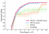
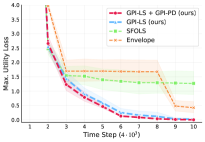
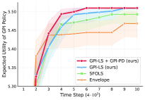
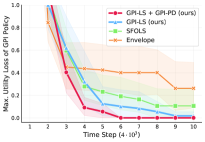
Figure 2. [Deep Sea Treasure Domain] Expected Utility and Maximum Utility Loss of each algorithm. Leftmost plots: performance of the best known policy. Rightmost plots: performance when following the GPI policy with respect to the known policies.

We evaluate the performance of our algorithms in challenging multi-objective tasks—both with discrete and continuous state and action spaces—and compare it with state-of-the-art MORL algorithms. We consider three environments Alegre et al. (2022b) with qualitatively different characteristics (see Fig. 1). We follow the performance evaluation methodology proposed in Zintgraf et al. (2015); Hayes et al. (2022), which focuses on utility-based metrics. These are relevant since they more directly reflect an algorithm’s performance with respect to a user’s preferences. Concretely, when evaluating a given algorithm, we compute the expected utility of its solutions: $\mathrm{EU}(\Pi)=\mathbb{E}_{\bm{\mathbf{w}}\sim\mathcal{W}}[\max_{\pi\in\Pi}v^{\pi}_{\bm{\mathbf{w}}}]$. We also quantify the maximum utility loss of an algorithm: $\mathrm{MUL}(\Pi)=\max_{\bm{\mathbf{w}}\in\mathcal{W}}(v^{*}_{\bm{\mathbf{w}}}-\max_{\pi\in\Pi}v^{\pi}_{\bm{\mathbf{w}}})$. We report the mean and its $95\%$ confidence interval over multiple random seeds.

Deep Sea Treasure. This is a classic MORL domain in which a submarine has to trade-off between collecting treasures and minimizing a time penalty (Fig. 1a). When evaluating our method in this setting, we employed a simplified, tabular version of GPI-PD (see Appendix). Recall that our GPI-LS algorithm (Alg. 1), unlike GPI-PD (Alg. 2), is model-free, does not perform Dyna planning steps, and uses a standard, unprioritized experience replay buffer with uniform sampling. We compare GPI-PD with two state-of-the-art competitors: Envelope MOQ-Learning Yang et al. (2019), and SFOLS Alegre et al. (2022a) (which uses OLS Roijers (2016); Mossalam et al. (2016) for selecting which weight vectors to train on).

In Fig. 2, we evaluate each algorithm’s expected utility (EU) and maximum utility (MUL) both (i) if each algorithm—when optimizing a given preference—follows its best known policy (two leftmost plots); and (ii) if each algorithm—when optimizing a given preference—follows the GPI policy derived from the known policies (two rightmost plots). We consider a setting where agents are constrained and have a limited budget of $4{,}000$ learning time steps per iteration. We now make a few important empirical observations, which hold for both above-mentioned settings (i and ii):

$\,\,\bullet$ The performance of the Envelope algorithm (both in terms of EU and MUL) has high variance since it trains on randomly-sampled weight vectors at each iteration. Furthermore, its asymptotic performance is always worse than our algorithms’ performances.

$\,\,\bullet$ SFOLS converges to a suboptimal CCS: it consistently adds suboptimal policies (the best ones it could discover under the training time constraints) to its CCS. As a result, SFOLS incorrectly prioritizes preferences.

$\,\,\bullet$ GPI-LS, by contrast, is consistently capable of identifying the most promising weight vectors, i.e., those with the highest guaranteed improvement according to Eq. (7). This allows it to always rapidly reach near-zero maximum utility loss. These results are consistent with Theorems 3.1 and 1, which formally ensure that GPI-LS always converges to optimal solutions and that it monotonically improves the quality of its solutions over time (up to approximation errors due to experimental statistics having been computed based on finite data points). When GPI-LS also employs experience prioritization (that is, when combined with GPI-PD), the resulting method produces even higher improvements at each iteration, thereby enhancing overall sample efficiency.

Minecart.

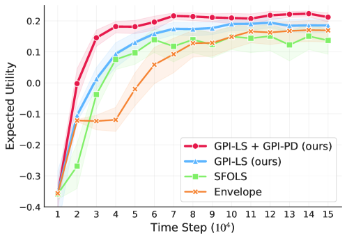
Expected Utility over 100 weight vectors from $\mathcal{W}$.

(a) Expected Utility over 100 weight vectors from $\mathcal{W}$.

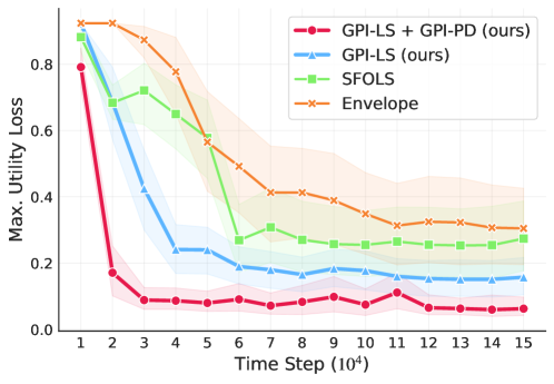
Maximum Utility Loss.

(b) Maximum Utility Loss.

Figure 3. [Minecart Domain] Performance evaluation.

Evaluation of the algorithms on the Minecart domain.

This domain involves controlling a cart (Fig. 1b) tasked with reaching ore mines, collecting and selling ores, and minimizing fuel consumption Abels et al. (2019). There are three conflicting objectives, representing the agent’s preferences for collecting each of the two types of ores, and for saving fuel. This is a continuous state space problem, and so we can directly deploy GPI-PD (Alg. 2); GPI-PD uses GPI both to prioritize weight vectors and experiences (Section 4.1). When comparing it with SFOLS and Envelope, we ensure that such competitors use the same neural network architecture and hyperparameters as GPI-PD, to allow for a fair comparison.

In Fig. 3(b), the performance of all algorithms follows a qualitatively similar behavior as observed in the Deep Sea Treasure experiment. Our methods (GPI-LS, and GPI-LS combined with GPI-PD) consistently identify optimal solutions, reach near-zero maximum utility loss, and achieve performance metrics that strictly dominate that of competitors. The Envelope algorithm is the least sample-efficient method during the first ten iterations—although it slightly surpasses the expected utility of SFOLS at the end of the learning process. These results further emphasize the importance of our weight prioritization technique (Section 3.1), which allows GPI-LS to allocate its training time to preferences whose performances are guaranteed to be improvable. As a result, GPI-LS outperforms the competing algorithms in terms of sample efficiency, and always converges to solutions with higher EU and MUL. Similarly, GPI-PD consistently reaches near-zero maximum utility loss.

MO-Hopper.

.

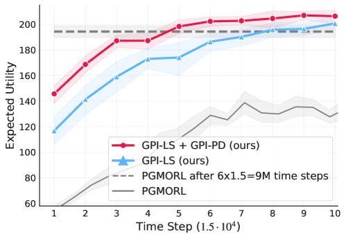
(a) Expected Utility over 100 weight vectors from $\mathcal{W}$.

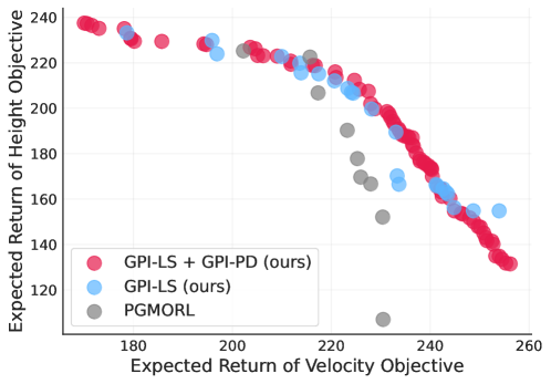
Pareto frontier encountered by each method.

(b) Pareto frontier produced by each method.

Figure 4. [MO-Hopper]: Performance evaluation.

Evaluation of the algorithms on the MO-Hopper domain.

This domain involves controlling a one-legged agent tasked with learning to hop while balancing two objectives: maximizing forward speed and jumping height. Unlike the previously-discussed domains, MO-Hopper operates over a continuous-action space. Neither Envelope nor SFOLS can tackle such a setting. For this reason, we compared our algorithms with a state-of-the-art MORL technique capable of dealing with continuous actions: PGMORL Xu et al. (2020). This is an evolutionary algorithm that assigns weight vectors to a population of agents (six, in our experiments, as in Xu et al. (2020)). Agents are trained in parallel using PPO Schulman et al. (2017). We extended our methods—both GPI-PD and GPI-LS—to deal with continuous actions by adapting the TD3 algorithm Fujimoto et al. (2018) to the MORL setting (see the Appendix). In Fig. 4(b), we compare the expected utility and Pareto frontiers generated by GPI-PD and PGMORL. Here, we analyze Pareto frontiers because we cannot compute the maximum utility loss exactly, since the optimal CCS is unknown. Pareto frontiers were computed by selecting all Pareto-efficient policies among those collected during 20 runs of the algorithms, and evaluating each such policy 5 times over 100 weight vectors. Once again, GPI-LS and GPI-PD have superior performance both in terms of expected utility and quality of the Pareto frontier. This is the case even though we allowed each of the six PGMORL agents to collect $1.5$ million experiences: they could interact with their environment ten times more often than our method/agent. Even then, GPI-PD (with or without using a learned model) consistently achieved higher expected utility (Fig. 4(a)) during learning, and converged to a final solution with superior performance. Fig. 4(b) depicts how the Pareto frontier identified by GPI-LS covers a broader range of behaviors that trade-off between the two objectives. This is made clear by observing that the points in the blue curve of Fig. 4(b) dominate the corresponding Pareto frontier of PGMORL. Similarly, GPI-LS, when combined with GPI-PD, also produces a Pareto frontier that dominates that of PGMORL with the exception of one value vector. Notice that because GPI-LS+GPI-PD prioritize both weight and experience selection, the resulting frontier is denser—it more thoroughly covers the space of all possible trade-offs between objectives.

6. Related Work

In this section, we briefly discuss some of the most relevant related work. For a complete discussion, see the Appendix.

Model-Free MORL. Several model-free MORL algorithms have been proposed in the literature  Van Moffaert and Nowé (2014); Parisi et al. (2017); Abdolmaleki et al. (2020); Hayes et al. (2022). Here, we discuss the ones that are most related to our work. In Abels et al. (2019), Abels et al. proposed training neural networks capable of predicting multi-objective action-value functions when conditioned on state and weight vector. Yang et al. Yang et al. (2019) extended the previously-mentioned approach to increase sample efficiency by introducing a novel operator for updating the action-value neural network parameters. Our method differs with respect to these in that (i) we introduced a novel, principled prioritization scheme to actively select weights on which the action-value network should be trained, in order to more rapidly learn a CCS (Section 3.1); and (ii) we introduced a principled prioritization method for sampling previous experiences for use in Dyna planning to accelerate learning optimal policies for particular agent preferences. The methods above, by contrast, use uniform sampling strategies that implicitly assume that all training data is equally important to rapidly identify optimal solutions. Alegre et al. Alegre et al. (2022a) showed how to use GPI in MORL settings, specifically in case the OLS algorithm is used to learn a CCS. Importantly, however, the heuristic used by OLS to select which weight vectors to train is based on upper bounds that are frequently exceedingly optimistic and loose. This means that OLS often focuses its training efforts on optimizing policies that do not necessarily improve the maximum utility loss incurred by the resulting CCS. Our method, by contrast, uses a technique for selecting which preferences to train on via a mathematically principled technique for determining a lower bound on performance improvements that are formally guaranteed to be achievable. This results in a novel active-learning approach that more accurately infers the ways by which a CCS can be rapidly improved. Xu et al. Xu et al. (2020) proposed an evolutionary algorithm that trains a population of agents specialized in different weight vectors. We used a single neural network conditioned on the weight vector to simultaneously model all policies in the CCS. Fig. 4(a) shows that our approach surpasses the performance of this algorithm, even when given ten times fewer environment interactions.

Model-Based MORL. Compared to model-free MORL algorithms, model-based MORL methods have been relatively less explored. Wiering et al. Wiering et al. (2014) introduced a tabular multi-objective dynamic programming algorithm. Yamaguchi et al. Yamaguchi et al. (2019) proposed an algorithm that learns models for predicting expected multi-objective reward vectors, rather than multi-objective Q-functions. Importantly, they tackle the average reward setting, rather than the cumulative discounted return setting. Yamaguchi et al. (2019) is limited to discrete state spaces and focuses its experiments on small MDPs with at most ten states. Similarly, Wiering et al. (2014) assumes both discrete and deterministic MOMDPs. Similarly, the model-based method in Agarwal et al. (2022) can tackle tabular, discrete settings—even though it supports non-linear utility functions. The methods proposed in Wang and Sebag (2012); Perez et al. (2015); Painter et al. (2020); Hayes et al. (2021) investigate multi-objective Monte Carlo tree search approaches, but unlike our algorithm, require prior access to known transition models of the MOMDP.

7. Conclusions

In this paper we introduced two principled prioritization methods that significantly improve sample efficiency, as well as the first model-based MORL algorithm capable of dealing with continuous state spaces. Both prioritization schemes we introduced were derived from properties of GPI and resulted in an effective, sample-efficient algorithm with important theoretical guarantees. In particular, we (i) proved strong convergence guarantees to an optimal solution in a finite number of steps, or to an $\epsilon$-optimal solution (for a bounded $\epsilon$) if the agent is limited and can only identify possibly sub-optimal policies; (ii) proved that our method is an anytime algorithm capable of monotonically improving the quality of the solution throughout the learning process; and (iii) formally defined a bound that characterizes the maximum utility loss incurred by partial solutions computed by our technique at any given iteration. Finally, we empirically showed that our algorithm outperforms state-of-the-art MORL algorithms in qualitatively different multi-objective problems, both with discrete and continuous state and action spaces. In future work, we would like to combine our algorithmic contributions with other types of model-based approaches, such as predecessor/backward models Chelu et al. (2020) and value equivalent models Grimm et al. (2021). We are also interested in extending our method to settings with non-linear utility functions.

This study was financed in part by the following Brazilian agencies: Coordenação de Aperfeiçoamento de Pessoal de Nível Superior - Brazil (CAPES) - Finance Code 001; CNPq (grants 140500/2021-9 and 304932/2021-3); and FAPESP/MCTI/CGI (grant 2020/05165-1). This research was partially supported by funding from the Flemish Government under the “Onderzoeksprogramma Artificiële Intelligentie (AI) Vlaanderen” program and the Research Foundation Flanders (FWO) [G062819N].

References

- (1)
- Abbas et al. (2020) Zaheer Abbas, Samuel Sokota, Erin Talvitie, and Martha White. 2020. Selective Dyna-Style Planning Under Limited Model Capacity. In Proceedings of the 37th International Conference on Machine Learning (Proceedings of Machine Learning Research, Vol. 119), Hal Daumé III and Aarti Singh (Eds.). PMLR, 1–10.
- Abdolmaleki et al. (2020) Abbas Abdolmaleki, Sandy Huang, Leonard Hasenclever, Michael Neunert, Francis Song, Martina Zambelli, Murilo Martins, Nicolas Heess, Raia Hadsell, and Martin Riedmiller. 2020. A distributional view on multi-objective policy optimization. In Proceedings of the 37th International Conference on Machine Learning (Proceedings of Machine Learning Research, Vol. 119). PMLR, 11–22.
- Abels et al. (2019) Axel Abels, Diederik M. Roijers, Tom Lenaerts, Ann Nowé, and Denis Steckelmacher. 2019. Dynamic weights in multi-objective deep reinforcement learning. In Proceedings of the 36th International Conference on Machine Learning, Vol. 97. International Machine Learning Society (IMLS), 11–20.
- Agarwal et al. (2022) Mridul Agarwal, Vaneet Aggarwal, and Tian Lan. 2022. Multi-Objective Reinforcement Learning with Non-Linear Scalarization. In Proceedings of the 21st International Conference on Autonomous Agents and Multiagent Systems (Virtual Event, New Zealand) (AAMAS ’22). International Foundation for Autonomous Agents and Multiagent Systems, Richland, SC, 9––17.
- Alegre et al. (2022a) Lucas N. Alegre, Ana L. C. Bazzan, and Bruno C. da Silva. 2022a. Optimistic Linear Support and Successor Features as a Basis for Optimal Policy Transfer. In Proceedings of the 39th International Conference on Machine Learning (Proceedings of Machine Learning Research, Vol. 162), Kamalika Chaudhuri, Stefanie Jegelka, Le Song, Csaba Szepesvari, Gang Niu, and Sivan Sabato (Eds.). PMLR, 394–413. https://proceedings.mlr.press/v162/alegre22a.html
- Alegre et al. (2022b) Lucas N. Alegre, Florian Felten, El-Ghazali Talbi, Grégoire Danoy, Ann Nowé, Ana L. C. Bazzan, and Bruno C. da Silva. 2022b. MO-Gym: A Library of Multi-Objective Reinforcement Learning Environments. In Proceedings of the 34th Benelux Conference on Artificial Intelligence BNAIC/Benelearn 2022.
- Barreto et al. (2018) Andre Barreto, Diana Borsa, John Quan, Tom Schaul, David Silver, Matteo Hessel, Daniel Mankowitz, Augustin Zidek, and Remi Munos. 2018. Transfer in Deep Reinforcement Learning Using Successor Features and Generalised Policy Improvement. In Proceedings of the 35th International Conference on Machine Learning (Proceedings of Machine Learning Research, Vol. 80), Jennifer Dy and Andreas Krause (Eds.). Stockholm, Sweden, 501–510.
- Barreto et al. (2017) Andre Barreto, Will Dabney, Remi Munos, Jonathan J Hunt, Tom Schaul, Hado P van Hasselt, and David Silver. 2017. Successor Features for Transfer in Reinforcement Learning. In Advances in Neural Information Processing Systems, I. Guyon, U. V. Luxburg, S. Bengio, H. Wallach, R. Fergus, S. Vishwanathan, and R. Garnett (Eds.), Vol. 30. Curran Associates, Inc.
- Barreto et al. (2020) André Barreto, Shaobo Hou, Diana Borsa, David Silver, and Doina Precup. 2020. Fast reinforcement learning with generalized policy updates. Proceedings of the National Academy of Sciences 117, 48 (2020), 30079–30087. https://doi.org/10.1073/pnas.1907370117
- Bellemare et al. (2020) Marc G. Bellemare, Salvatore Candido, Pablo Samuel Castro, Jun Gong, Marlos C. Machado, Subhodeep Moitra, Sameera S. Ponda, and Ziyu Wang. 2020. Autonomous navigation of stratospheric balloons using reinforcement learning. Nature 588, 7836 (01 Dec 2020), 77–82. https://doi.org/10.1038/s41586-020-2939-8
- Borsa et al. (2019) Diana Borsa, André Barreto, John Quan, Daniel J. Mankowitz, Rémi Munos, H. V. Hasselt, D. Silver, and T. Schaul. 2019. Universal Successor Features Approximators. In Proceedings of the 7th International Conference on Learning Representations (ICLR).
- Buckman et al. (2018) Jacob Buckman, Danijar Hafner, George Tucker, Eugene Brevdo, and Honglak Lee. 2018. Sample-Efficient Reinforcement Learning with Stochastic Ensemble Value Expansion. In Advances in Neural Information Processing Systems, S. Bengio, H. Wallach, H. Larochelle, K. Grauman, N. Cesa-Bianchi, and R. Garnett (Eds.), Vol. 31. Curran Associates, Inc.
- Chelu et al. (2020) Veronica Chelu, Doina Precup, and Hado P van Hasselt. 2020. Forethought and Hindsight in Credit Assignment. In Advances in Neural Information Processing Systems, H. Larochelle, M. Ranzato, R. Hadsell, M. F. Balcan, and H. Lin (Eds.), Vol. 33. Curran Associates, Inc., 2270–2281.
- Chua et al. (2018) Kurtland Chua, Roberto Calandra, Rowan McAllister, and Sergey Levine. 2018. Deep Reinforcement Learning in a Handful of Trials Using Probabilistic Dynamics Models. In Proceedings of the 32nd International Conference on Neural Information Processing Systems (Montréal, Canada) (NIPS’18). Curran Associates Inc., Red Hook, NY, USA, 4759––4770.
- Deisenroth and Rasmussen (2011) Marc Peter Deisenroth and Carl Edward Rasmussen. 2011. PILCO: A Model-Based and Data-Efficient Approach to Policy Search. In Proceedings of the 28th International Conference on International Conference on Machine Learning (ICML) (Bellevue, Washington, USA) (ICML’11). Omnipress, Madison, WI, USA, 465–472.
- D’Oro and Jaskowski (2020) Pierluca D’Oro and Wojciech Jaskowski. 2020. How to Learn a Useful Critic? Model-based Action-Gradient-Estimator Policy Optimization. In Advances in Neural Information Processing Systems 33. Virtual. https://proceedings.neurips.cc/paper/2020/hash/03255088ed63354a54e0e5ed957e9008-Abstract.html
- Feinberg et al. (2018) Vladimir Feinberg, Alvin Wan, Ion Stoica, Michael I. Jordan, Joseph E. Gonzalez, and Sergey Levine. 2018. Model-Based Value Estimation for Efficient Model-Free Reinforcement Learning. CoRR abs/1803.00101 (2018). arXiv:1803.00101 http://arxiv.org/abs/1803.00101
- Fujimoto et al. (2018) Scott Fujimoto, Herke Hoof, and David Meger. 2018. Addressing Function Approximation Error in Actor-Critic Methods. In Proceedings of the 35th International Conference on Machine Learning. 1582–1591.
- Fujimoto et al. (2020) Scott Fujimoto, David Meger, and Doina Precup. 2020. An Equivalence between Loss Functions and Non-Uniform Sampling in Experience Replay. In Advances in Neural Information Processing Systems, H. Larochelle, M. Ranzato, R. Hadsell, M. F. Balcan, and H. Lin (Eds.), Vol. 33. Curran Associates, Inc., 14219–14230.
- Grimm et al. (2021) Christopher Grimm, André Barreto, Gregory Farquhar, David Silver, and Satinder Singh. 2021. Proper Value Equivalence. In Proceedings of the 35th Conference on Neural Information Processing Systems. Sydney, Australia.
- Hayes et al. (2022) Conor F. Hayes, Roxana Rădulescu, Eugenio Bargiacchi, Johan Källström, Matthew Macfarlane, Mathieu Reymond, Timothy Verstraeten, Luisa M. Zintgraf, Richard Dazeley, Fredrik Heintz, Enda Howley, Athirai A. Irissappane, Patrick Mannion, Ann Nowé, Gabriel Ramos, Marcello Restelli, Peter Vamplew, and Diederik M. Roijers. 2022. A practical guide to multi-objective reinforcement learning and planning. Autonomous Agents and Multi-Agent Systems 36, 1 (13 Apr 2022), 26. https://doi.org/10.1007/s10458-022-09552-y
- Hayes et al. (2021) Conor F. Hayes, Mathieu Reymond, Diederik M. Roijers, Enda Howley, and Patrick Mannion. 2021. Risk Aware and Multi-Objective Decision Making with Distributional Monte Carlo Tree Search. In Proceedings of the 20th International Conference on Autonomous Agents and Multiagent Systems.
- Janner et al. (2019) Michael Janner, Justin Fu, Marvin Zhang, and Sergey Levine. 2019. When to Trust Your Model: Model-Based Policy Optimization. In Advances in Neural Information Processing Systems (NIPS) 32, H. Wallach, H. Larochelle, A. Beygelzimer, F. d’ Alché-Buc, E. Fox, and R. Garnett (Eds.). Curran Associates, Inc., 12519–12530. http://papers.nips.cc/paper/9416-when-to-trust-your-model-model-based-policy-optimization.pdf
- Kaiser et al. (2020) Lukasz Kaiser, Mohammad Babaeizadeh, Piotr Miłos, Błażej Osiński, Roy H Campbell, Konrad Czechowski, Dumitru Erhan, Chelsea Finn, Piotr Kozakowski, Sergey Levine, Afroz Mohiuddin, Ryan Sepassi, George Tucker, and Henryk Michalewski. 2020. Model Based Reinforcement Learning for Atari. In Proceeding of the 8th International Conference on Learning Representations.
- Lai et al. (2021) Hang Lai, Jian Shen, Weinan Zhang, Yimin Huang, Xing Zhang, Ruiming Tang, Yong Yu, and Zhenguo Li. 2021. On Effective Scheduling of Model-based Reinforcement Learning. In Proceedings of the 35th Conference on Neural Information Processing Systems, A. Beygelzimer, Y. Dauphin, P. Liang, and J. Wortman Vaughan (Eds.). https://openreview.net/forum?id=z36cUrI0jKJ
- Lin (1992) Long-Ji Lin. 1992. Self-improving reactive agents based on reinforcement learning, planning and teaching. Machine Learning 8, 3 (01 May 1992), 293–321. https://doi.org/10.1007/BF00992699
- Moerland et al. (2020) Thomas M. Moerland, Joost Broekens, and Catholijn M. Jonker. 2020. Model-based Reinforcement Learning: A Survey. CoRR abs/2006.16712 (2020). arXiv:2006.16712 https://arxiv.org/abs/2006.16712
- Moore and Atkeson (1993) Andrew W. Moore and Christopher G. Atkeson. 1993. Prioritized Sweeping: Reinforcement Learning With Less Data and Less Time. Machine Learning 13 (1993), 103–130.
- Mossalam et al. (2016) Hossam Mossalam, Yannis M. Assael, Diederik M. Roijers, and Shimon Whiteson. 2016. Multi-Objective Deep Reinforcement Learning. CoRR abs/1610.02707 (2016). arXiv:1610.02707 http://arxiv.org/abs/1610.02707
- Painter et al. (2020) Michael Painter, Bruno Lacerda, and Nick Hawes. 2020. Convex Hull Monte-Carlo Tree-Search. In Proceedings of the 30th International Conference on Automated Planning and Scheduling (ICAPS). AAAI Press, 217–225.
- Pan et al. (2022) Yangchen Pan, Jincheng Mei, Amir massoud Farahmand, Martha White, Hengshuai Yao, Mohsen Rohani, and Jun Luo. 2022. Understanding and Mitigating the Limitations of Prioritized Experience Replay. In Proceedings of the 38th Conference on Uncertainty in Artificial Intelligence. https://openreview.net/forum?id=HBlNGvIicg9
- Pan et al. (2019) Yangchen Pan, Hengshuai Yao, Amir-massoud Farahmand, and Martha White. 2019. Hill Climbing on Value Estimates for Search-control in Dyna. In Proceedings of the 28th International Joint Conference on Artificial Intelligence. ijcai.org, Macao, China, 3209–3215. https://doi.org/10.24963/ijcai.2019/445
- Pan et al. (2018) Yangchen Pan, Muhammad Zaheer, Adam White, Andrew Patterson, and Martha White. 2018. Organizing Experience: A Deeper Look at Replay Mechanisms for Sample-Based Planning in Continuous State Domains. In Proceedings of the 27th International Joint Conference on Artificial Intelligence (Stockholm, Sweden) (IJCAI’18). AAAI Press, 4794––4800.
- Parisi et al. (2017) S. Parisi, M. Pirotta, and J. Peters. 2017. Manifold-based multi-objective policy search with sample reuse. Neurocomputing 263 (2017), 3–14. https://doi.org/10.1016/j.neucom.2016.11.094 Special Issue on Multi-Objective Reinforcement Learning.
- Perez et al. (2015) Diego Perez, Sanaz Mostaghim, Spyridon Samothrakis, and Simon M. Lucas. 2015. Multiobjective Monte Carlo Tree Search for Real-Time Games. IEEE Transactions on Computational Intelligence and AI in Games 7, 4 (2015), 347–360. https://doi.org/10.1109/TCIAIG.2014.2345842
- Puterman (2005) Martin L. Puterman. 2005. Markov Decision Processes: Discrete Stochastic Dynamic Programming. Wiley–Interscience, New York, NY, USA.
- Roijers (2016) Diederik Roijers. 2016. Multi-Objective Decision-Theoretic Planning. Ph.D. Dissertation. University of Amsterdam.
- Roijers et al. (2013) Diederik M. Roijers, Peter Vamplew, Shimon Whiteson, and Richard Dazeley. 2013. A Survey of Multi-Objective Sequential Decision-Making. J. Artificial Intelligence Research 48, 1 (Oct. 2013), 67–113.
- Schaul et al. (2016) Tom Schaul, John Quan, Ioannis Antonoglou, and David Silver. 2016. Prioritized Experience Replay. In Proceedings of the 33rd International Conference on Learning Representations. Puerto Rico.
- Schulman et al. (2017) John Schulman, Filip Wolski, Prafulla Dhariwal, Alec Radford, and Oleg Klimov. 2017. Proximal Policy Optimization Algorithms. CoRR abs/1707.06347 (2017). arXiv:1707.06347 http://arxiv.org/abs/1707.06347
- Silver et al. (2017) David Silver, Julian Schrittwieser, Karen Simonyan, Ioannis Antonoglou, Aja Huang, Arthur Guez, Thomas Hubert, Lucas Baker, Matthew Lai, Adrian Bolton, Yutian Chen, Timothy Lillicrap, Fan Hui, Laurent Sifre, George van den Driessche, Thore Graepel, and Demis Hassabis. 2017. Mastering the game of Go without human knowledge. Nature 550, 7676 (01 Oct 2017), 354–359. https://doi.org/10.1038/nature24270
- Sutton (1990) Richard S. Sutton. 1990. Integrated Architectures for Learning, Planning, and Reacting Based on Approximating Dynamic Programming. In Proceedings of the 7th International Conference on Machine Learning. 216–224.
- Sutton and Barto (2018) Richard S. Sutton and Andrew G. Barto. 2018. Reinforcement learning: An introduction (second ed.). The MIT Press.
- Van Moffaert and Nowé (2014) Kristof Van Moffaert and Ann Nowé. 2014. Multi-Objective Reinforcement Learning Using Sets of Pareto Dominating Policies. J. Mach. Learn. Res. 15, 1 (Jan. 2014), 3483–3512.
- Van Seijen and Sutton (2015) Harm Van Seijen and Rich Sutton. 2015. A Deeper Look at Planning as Learning from Replay. In Proceedings of the 32nd International Conference on Machine Learning (Proceedings of Machine Learning Research, Vol. 37), Francis Bach and David Blei (Eds.). PMLR, Lille, France, 2314–2322.
- Van Seijen and Sutton (2013) Harm Van Seijen and Richard S. Sutton. 2013. Efficient Planning in MDPs by Small Backups. In Proceedings of the 30th International Conference on International Conference on Machine Learning (Atlanta, GA, USA) (ICML’13). JMLR.org, III–361––III–369.
- Wang and Sebag (2012) Weijia Wang and Michèle Sebag. 2012. Multi-objective Monte-Carlo Tree Search. In Proceedings of the Asian Conference on Machine Learning (Proceedings of Machine Learning Research, Vol. 25), Steven C. H. Hoi and Wray Buntine (Eds.). PMLR, Singapore Management University, Singapore, 507–522. https://proceedings.mlr.press/v25/wang12b.html
- Wiering et al. (2014) Marco A. Wiering, Maikel Withagen, and Mădălina M Drugan. 2014. Model-based multi-objective reinforcement learning. In 2014 IEEE Symposium on Adaptive Dynamic Programming and Reinforcement Learning (ADPRL). 1–6. https://doi.org/10.1109/ADPRL.2014.7010622
- Wurman et al. (2022) Peter R. Wurman, Samuel Barrett, Kenta Kawamoto, James MacGlashan, Kaushik Subramanian, Thomas J. Walsh, Roberto Capobianco, Alisa Devlic, Franziska Eckert, Florian Fuchs, Leilani Gilpin, Piyush Khandelwal, Varun Kompella, HaoChih Lin, Patrick MacAlpine, Declan Oller, Takuma Seno, Craig Sherstan, Michael D. Thomure, Houmehr Aghabozorgi, Leon Barrett, Rory Douglas, Dion Whitehead, Peter Dürr, Peter Stone, Michael Spranger, and Hiroaki Kitano. 2022. Outracing champion Gran Turismo drivers with deep reinforcement learning. Nature 602, 7896 (01 Feb 2022), 223–228. https://doi.org/10.1038/s41586-021-04357-7
- Xu et al. (2020) Jie Xu, Yunsheng Tian, Pingchuan Ma, Daniela Rus, Shinjiro Sueda, and Wojciech Matusik. 2020. Prediction-Guided Multi-Objective Reinforcement Learning for Continuous Robot Control. In Proceedings of the 37th International Conference on Machine Learning (ICML).
- Yamaguchi et al. (2019) Tomohiro Yamaguchi, Shota Nagahama, Yoshihiro Ichikawa, and Keiki Takadama. 2019. Model-Based Multi-objective Reinforcement Learning with Unknown Weights. In Human Interface and the Management of Information. Information in Intelligent Systems, Sakae Yamamoto and Hirohiko Mori (Eds.). Springer International Publishing, Cham, 311–321.
- Yang et al. (2019) Runzhe Yang, Xingyuan Sun, and Karthik Narasimhan. 2019. A Generalized Algorithm for Multi-Objective Reinforcement Learning and Policy Adaptation. In Advances in Neural Information Processing Systems 32, H. Wallach, H. Larochelle, A. Beygelzimer, F. d’ Alché-Buc, E. Fox, and R. Garnett (Eds.). 14610–14621.
- Zintgraf et al. (2015) Luisa M. Zintgraf, Timon V. Kanters, Diederik M. Roijers, Frans A. Oliehoek, and Philipp Beau. 2015. Quality Assessment of MORL Algorithms: A Utility-Based Approach. In Benelearn 2015: Proceedings of the 24th Annual Machine Learning Conference of Belgium and the Netherlands.