Abstract
The study of compact object populations has come a long way since the determination of the mass of the Hulse–Taylor pulsar, and we now count on more than 150 known Galactic neutron stars and black hole masses, as well as another 180 objects from binary mergers detected from gravitational-waves by the Ligo–Virgo–KAGRA Collaboration. With a growing understanding of the variety of systems that host these objects, their formation, evolution and frequency, we are now in a position to evaluate the statistical nature of these populations, their properties, parameter correlations and long-standing problems, such as the maximum mass of neutron stars and the black hole lower mass gap, to a reasonable level of statistical significance. Here, we give an overview of the evolution and current state of the field and point to some of its standing issues. We focus on Galactic black holes, and offer an updated catalog of 35 black hole masses and orbital parameters, as well as a standardized procedure for dealing with uncertainties.
keywords:
neutron stars; black holes; mass distribution; formation channels1 \issuenum1 \articlenumber0 \externaleditorAcademic Editor: Jaziel Goulart Coelho, Rita C. Anjos \datereceived29 November 2022 \daterevised22 December 2022 \dateaccepted28 December 2022 \datepublished \hreflinkhttps://doi.org/ \TitleAn Overview of Compact Star Populations and Some of Its Open Problems \TitleCitationAn Overview of Compact Star Populations and Some of Its Open Problems \AuthorLucas M. de Sá 1\orcidA, Antônio Bernardo 1\orcidB, Riis R. A. Bachega 1\orcidC, Livia S. Rocha1\orcidD, Pedro H. R. S. Moraes 2\orcidEand Jorge E. Horvath 1*\orcidF \AuthorNames Lucas M. de Sá, Antônio Bernardo, Riis R. A. Bachega, Lívia S. Rocha, Pedro H. R. S. Moraes and Jorge E. Horvath \AuthorCitationde Sá, Lucas M.; Bernardo, Antônio; Bachega, Riis R.A.; Rocha, Livia S.; Moraes, Pedro H.R.S.; Horvath, Jorge E. \corresCorrespondence: foton@iag.usp.br; Tel.: 55-11-30912710
1 Introduction
The recognition that extreme states of matter constitute the endpoints of Stellar Evolution is one of the most important achievements of the 20th century. In fact, all the concepts and developments of Stellar Evolution started as such in the 19th century, and evolved symbiotically with the new exciting “modern” Physics, General Relativity, Nuclear Physics, Quantum Mechanics, and Statistical Mechanics. Stellar Evolution is their legitimate daughter and combined many things to create a consistent and predictive picture of how stars evolve.
This happy confluence is particularly important for the compact remnants, leftovers of massive stars in which the final stages prompted matter to show its ultimate nature. This is how the idea of neutron stars (NS) was raised, and although the black hole (BH) concept followed a different path, their recognition as stellar remnants unifies the two classes as stellar corpses.
Neutron stars are now recognized to come in many varieties. In addition to the celebrated pulsar group, dim isolated neutron stars (also known as XDINSs) Walter et al. (1996); Zampieri et al. (2001); Turolla (2009); Ertan et al. (2014), magnetars Esposito et al. (2021), Compact Central Objects in supernova remnants De Luca (2017); Mayer and Becker (2021); Ho (2013); Ho et al. (2021), Rotating Radio Transients Abhishek et al. (2022); Keane and McLaughlin (2011) and some amazing new detections tentatively labeled as Ultra-Slow Magnetars Hurley-Walker et al. (2022) form a full family which we would like to understand as a whole. We shall briefly address this issue below.
Galactic black holes, much as has been the case since the confirmation of the first one in Cygnus X-1, are observed generally as components of X-ray binaries, in most cases with a dwarf companion, although a few systems with giant companions are known. This means that most known BH masses have been determined from dynamical parameters (orbital period, mass function, mass ratio), which have been compiled in current catalogs such as BlackCAT111https://www.astro.puc.cl/BlackCAT/ Corral-Santana et al. (2016) and WATCHDOG222https://sites.ualberta.ca/~btetaren/ Tetarenko et al. (2016). In recent years, however, novel techniques, such as the study of quasi-periodic oscillations Ingram and Motta (2019) and of gravitational microlensing Lam et al. (2022); Sahu et al. (2022), have allowed for masses to be constrained in different ways. The greatest example of this lies in the case of extragalactic black holes, over 100 of which have had their masses constrained from gravitational-wave (GW) observations of compact object mergers by the LIGO-Virgo-KAGRA Collaboration (LVK) 333https://www.ligo.caltech.edu/page/ligo-scientific-collaboration. In what follows, we will deal in detail with the current 35 well-constrained Galactic BH masses, and also briefly overview and compare them to the extragalactic BH mass distribution observed so far.
The last twenty years or so produced in fact a large body of evidence in which the simplest theoretical expectations serve as an overall framework only. The process of massive star collapse, for example, has been deeply explored and there are now different perspectives on how exactly it happens, and particularly on which outcome can be expected from them Burrows and Vartanyan (2021); Ertl et al. (2020).
At the same time, the determination of masses of NSs and BHs with good accuracy in larger samples has allowed a better glimpse of the astrophysical processes that lead to their birth. This is indeed a long-term task, since many complicated issues in the evolution of progenitors and explosions themselves are involved. We shall not address these issues here, but rather indicate some recent works that illustrate the state-of-the-art understanding of them. The connection with the compact star features is also dependent on the binarity of forming systems to a high degree, and in fact it is in binaries (in which one of the members is generally non-compact) where most of the masses (and some radii for NSs) have been measured. Last, but not least, the production of NSs by accretion induced collapse Tauris et al. (2013); Wang and Liu (2020); Wang et al. (2022) is not properly understood but may be important for the whole picture, as we shall see. All these issues are entangled when we have to address, for example, the suggested absence of objects between and , a paucity called lower mass gap in the literature Bailyn et al. (1998); Özel et al. (2010); Farr et al. (2011); Fryer et al. (2012); Belczynski et al. (2012). We shall address the existence of a mass gap below according to analyses of the latest data Farah et al. (2022); de Sá et al. (2022); Ye and Fishbach (2022). Finally, a novel form of “seeing” compact objects is the now systematic monitoring of gravitational-wave events. Great insights on NS matter have been gathered from the event GW170817 and a substantial set of compact binary masses has been collected through three LVK runs, and these we also discuss briefly.
We start in Section 2 by offering a brief overview of current issues under study with regard to NSs, including their demographics, maximum mass, mass distribution and radius measurements. We follow this in Section 3 with a more thorough discussion of the current state of BH observations, in particular that of Galactic objects, where we present, case-by-case, an updated catalog of 35 known masses, calculated in a standardized way from dynamical parameters. We display in Section 3.5 the resulting full Galactic BH mass distribution, and briefly discuss and compare it to the extragalactic distribution from LVK. Finally, we summarize the evolution and current state of the lower mass gap problem in Section 3.6. Our concluding remarks are presented in Section 4.
2 Neutron Stars
Neutron stars were predicted simultaneously with the discovery of the neutron itself Landau (1932), and related to collapsing/exploding stars by Baade and Zwicky (1934) without any real proof of their existence. “Real” neutron stars became a reality 30 years later, when the first pulsating radio sources were discovered Hewish et al. (1968) and the present model (or close to it) was put forward by Pacini (1968) and Gold (1968). However, it became clear over the years that not all NSs pulse, since for that rapid rotation and intense magnetic fields are necessary, according to the basic model in which the torque is given by the electromagnetic emission and scales . In addition, new classes of NSs have been identified, and other properties such as masses and radii measured with increasing precision. We shall briefly point out the main features of each group, the expected demographics and the inferred physical quantities in the following (for a recent full review, see Horvath et al. (2022)).
2.1 Neutron Star Demographics
It is commonplace understanding that NSs are born in massive star supernova explosions. However, it is almost certain that contributions from the explosions of “low-mass” massive stars, in the range of 8–, which are thought to undergo electron capture onto an O-Ne-Mg core and leave “light” NSs is an important channel, since progenitors in this mass range are abundant. In addition, the rate of accretion induced collapses (AICs), either in their single-degenerate or double-degenerate (merger) versions, is uncertain but must be added to the total if some NSs are formed by them (Tauris et al., 2013; Wang and Liu, 2020; Wang et al., 2022). Simply multiplying by the Galactic lifetime the proper core–collapse supernova rate extrapolated from observations in galaxies similar to the Milky Way gives a number of NSs births of over the whole life of the Galaxy Bisnovatyi-Kogan (1992). The large group of active pulsars today has been estimated to be around Lyne et al. (1985); Dirson et al. (2022), although this number quite depends on the birth parameters and evolution of magnetic fields. However, it is highly unlikely that the estimate is wrong by an order of magnitude, leading to the conclusion that most of the Galactic NSs are not pulsars, but instead belong to one of several classes that may be termed “hidden”, which we describe below. These are NSs that may or may not have functioned as pulsars in the past, but the presence of which would be much more difficult to establish today. Attempts to unify all NSs have been presented before Kaspi (2010), but as we shall see, new puzzling detections and unresolved problems are still ubiquitous.
Some well-known NSs are natural candidates for the large “hidden” group. These include the central compact objects (CCOs) in a few supernova remnants without detected pulsations De Luca (2017); Mayer and Becker (2021). Most of the population is likely to have faded away due to its old age, well beyond the scale, and therefore to establish their presence and statistics is quite difficult, although progress has been made; see, e.g., (Ho, 2013; Ho et al., 2021).
Detected between 1996, with the observation of RX J1856.4–3754 by Walter et al. (1996), and 2001, when RBS 1774 was first observed by Zampieri et al. (2001), the subpopulation termed the Magnificent Seven or X-ray Dim Isolated Neutron Stars (XDINSs), in addition to the isolated NS Calvera Rutledge et al. (2008), consists of relatively close, blackbody-like cooling NSs (Potekhin et al., 2015) that were once considered the tip of the population iceberg. However, pulsations and non-zero period derivatives were detected over time, proving that they are actually middle-aged objects Turolla (2009); Ertan et al. (2014). Nevertheless, the paucity of this type of NS is somewhat unexpected, and no additional candidates (except for Calvera) were added over many years.
Another subpopulation which was identified unexpectedly is that of Rotating Radio Transients (RRATs), emitting occasionally isolated pulses of a few ms and going silent for days or more (Keane and McLaughlin, 2011). This narrow duty cycle makes them virtually invisible most of the time, and therefore their number could be very large. A simple estimate from the sources already known is
| (1) |
where is the duty fraction and all other uncertainties have been set to unity multiplication factors. We see that their number could be larger than the estimated number of ordinary radio pulsars, but it is unlikely that the bulk of born NSs can be accommodated. In fact, the construction of coherent solutions for the sporadic pulses allowed an estimate of some of the period derivatives , and thus an estimate of the characteristic spin-down ages. They seem to be not too different from ordinary pulsars in this aspect (see Figure 1), and it has been conjectured that for some reason the “spark” leading to a pulse is not always operating, like they do in the pulsar case (Abhishek et al., 2022). Of course, we do not know enough about the origin of pulses to discard or prove these ideas.
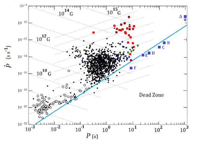
A third subgroup of importance is that of the so-called magnetars, objects in which the emission is related to the existence of a large magnetic field, dominating the energetics of the rotation (i.e., satisfying that the X-ray luminosity exceeds the rotational energy ); see, for a recent review, (Esposito et al., 2021). Magnetars seem to possess magnetic fields a few orders of magnitude larger than the ordinary pulsar variety. The natural question is whether there is a continuum of NSs, in the sense that the magnetic fields are generated by a continuous distribution, or if there is some kind of gap in this quantity instead. The presence of transition pulsars, with magnetic fields as high as some identified magnetars seems to argue in favor of the former. The existence of “low-field” magnetars Turolla and Esposito (2013) is also suggestive of a continuum (Figure 1). In this way, the magnetar group was defined as the NSs in which the emission is powered by the magnetic field, irrespective of the precise value of its intensity.
The latest news about the NSs population include the discovery of progressively longer period pulsars (Caleb et al., 2022) and magnetars (Hurley-Walker et al., 2022) (see caption of Figure 1). These unexpected objects are not only below the “classical” death line, but also challenge a definite division between the two groups. At some point the energy condition is employed to separate them, but otherwise their position in the plane does not allow one to establish a clear classification. In addition, the first (and unique up to now) pulsar-like white dwarf AR Scorpii (object B in Figure 1) (Buckley et al., 2017) is included in this group. For now, the latter is just a singularity, but it is likely that a subpopulation could be found, although unrelated to the NSs demographics.
What are the main questions one can ask about these subpopulations and their relationships? The list is quite extensive, and we shall only point out some of them to contribute to this ongoing task.
-
•
Do magnetic fields decay?
This question is one of the oldest, and has been answered differently over the years. The idea that there must be a decay of the field within is quite popular, as discussed and modeled by Viganò et al. (2013) for a diverse set of 40 sources including, e.g., the already mentioned magnetars, CCOs and XDINSs; see also, for a review, Igoshev et al. (2021). However, objects of this age still show substantial magnetic fields, and the oldest ones (“black widows”, several Gyr old according to evolution calculations Benvenuto et al. (2014)) reinforce this picture. Magnetic fields may decay partially to a “bottom field”, but not completely and therefore many evolutionary trajectories in the plane proposed to explain the transit and parenthood of many subpopulations could be misleading. Theoretical calculations support this kind of picture Mendes et al. (2018).
-
•
Which is the relationship between all these subpopulations?
The idea that some subpopulations are just an evolutionary stage leading to some other type is behind all the attempts of unification Kaspi (2010), in one way or another. It is perhaps useful trying to establish which are the youngest and oldest objects. Here, we face a very general problem: in many cases, the age of the object is calculated with the characteristic age, and its magnetic field with the inversion of the electromagnetic torque equation (yielding ). However, it is clear by several lines of argument that this is probably an oversimplified picture. Braking indexes are not what the ideal electromagnetic torque predicts Igoshev and Popov (2020), and there is evidence for variations of the torque itself with time Allen and Horvath (1997). Several ideas have been put forward to link subpopulations; the analysis by Yoneyama et al. (2019), for example, supported the idea that XDINSs are old magnetars, not common-type pulsars. Typical ages of magnetars (soft gamma repeaters Hurley (2010) and anomalous X-ray pulsars Kaspi (2007)) are , and some support for young ages comes from their associations with young supernova remnants. Other kinships have been suggested; for instance, Keane (2016) points out that, from empirical grounds, RRATs and Fast Radio Bursts sources are hardly distinguishable. The clue for this association, and the possible relation with ordinary pulsars which are side by side with RRATs in the diagram, is, of course, a deeper and solid understanding of the short radio pulse emission, and of ordinary pulsar emission in general (Kaspi and Kramer (2016) present an overview of how these different manifestations of NSs relate to pulsars).
-
•
Are the new objects old magnetars?
The ultra-slow magnetars should be, logically thinking, a latter stage in which they have cooled and braked to very long periods. However, their inferred magnetic fields are very high, and according to conventional wisdom, they should not be that old indeed. Are they actually related? Beniamini et al. (2022) have argued that there must be a large population of ultra-slow magnetars in the galaxy, stressing the resiliency of magnetic fields. Is there a real difference between RRATs and ultra-slow magnetars? In addition, is it a complete coincidence that the “WD pulsar” stands nearby other confirmed NSs of this group? It is premature to give definitive answers to these and other important questions
2.2 Neutron Star Mass Distribution
The NS mass sample has 105 members now, with the addition of a few recent observations. An analysis of a slightly smaller sample (95 objects), presented in de Sá et al. (2022), was discussed in full by Rocha et al. (2021), and we shall highlight the main features for completeness.
The first important thing is that, as agreed by several groups Postnov and Prokhorov (2001); Valentim et al. (2011); Özel and Freire (2016); Kiziltan et al. (2013); Zhang et al. (1997); Alsing et al. (2018), the sample has a multimodal structure, with at least two mass scales. The analysis of Rocha et al. (2021) was performed assuming a Gaussian parametrization with components, of the type
| (2) |
where and are the mean and standard deviation of the i-th component , and is its relative weight, satisfying the normalization condition .
As discussed in Horvath et al. (2022), the preferred figures for both Anderson–Darling and Kolmogorov–Smirnov frequentist tests are the ones appearing in Table 1.
| \PreserveBackslash Model | \PreserveBackslash | \PreserveBackslash | \PreserveBackslash K–S | \PreserveBackslash A–D | \PreserveBackslash Recommendation |
|---|---|---|---|---|---|
| \PreserveBackslash Unimodal | \PreserveBackslash 1.48 | \PreserveBackslash 0.35 | \PreserveBackslash 0.025 | \PreserveBackslash 0.032 | \PreserveBackslash Reject |
| \PreserveBackslash Bimodal | \PreserveBackslash 1.38, 1.84 | \PreserveBackslash 0.15, 0.35 | \PreserveBackslash 0.971 | \PreserveBackslash 0.990 | \PreserveBackslash Do not reject |
| \PreserveBackslash Trimodal | \PreserveBackslash 1.25, 1.40, 1.89 | \PreserveBackslash 0.09, 0.14, 0.30 | \PreserveBackslash 0.974 | \PreserveBackslash 0.953 | \PreserveBackslash Do not reject |
The -values indicate a strong rejection of a “single mass” hypothesis (labeled as “Unimodal”) and hence the confirmation of a structured mass distribution. It should be noted that a peak at 1.25 is expected, related to the NSs produced in electron-capture supernovae, but the analysis does not reveal clear evidence for it. The low-mass NSs appear equally likely to be part of the tail of the strong maximum at 1.38, which is narrower than the second one around 1.8. Massive NSs belong to the latter fully.
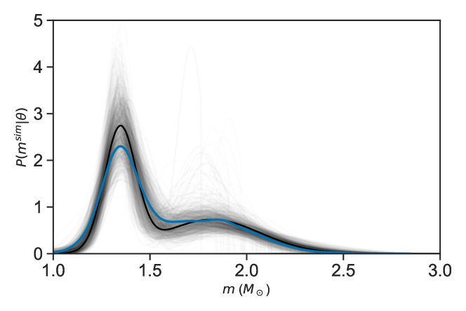
To visualize the form of the mass distribution, we have drawn 1000 posterior samples from the master sample discussed in Horvath et al. (2022), and taken their mean to compare with the maximum a posteriori distribution obtained. The result confirms the presence of two maxima as explained.
A Bayesian analysis was implemented to cross-check these results. Again, the Bayesian likelihood is much higher for the bimodal distribution, and the mean and standard deviation of the two peaks quite similar, , and , . This reinforces the conclusion that there are at least two peaks, and probably a third one “blended” with the objects at 1.38, but not a single mass (called sometimes “canonical” in the literature, a name that is now not recommended).
It is much more difficult to attach definite formation events to these Gaussian peaks, although in the long run it will be a rewarding task. The maximum mass achievable by a real NS, , which has as its upper bound the Rhoades–Ruffini limit of 3.2 Rhoades and Ruffini (1974), should be obtained in a large sample having a statistical upper mass boundary , since in this case, and provided the sample is not biased, . At the present time, we can say that was studied using the current sample and turns out to be both by a simpler estimate of the second peak (Figure 2), and also by a Bayesian approach, both with and without an upper truncation mass introduced as an independent quantity (Rocha et al., 2021).
On the one hand, such a large value of is at odds with many estimates based on the analysis of the merged object in GW170817, which yield values near 2.1–2.2 Margalit and Metzger (2017); Rezzolla et al. (2018); Ruiz et al. (2018); Shibata et al. (2019). On the other hand, (Ai et al., 2020) have also found from GW170817 that might be as high as , even if the remnant is born as a uniformly-rotating NS. Rocha et al. (2021) aim to avoid limitations arising from estimates based on single sources by obtaining their from a Bayesian analysis of the full sample of Galactic NS masses, which makes their resulting large mass robust. There are also several candidates that would be above the typical inferred value, and one definite quite reliable determination of 2.35 0.17 (Romani et al., 2021) which challenges a low limit and has already pushed more recent works to allow for a higher than previously conducted Ecker and Rezzolla (2022). A high makes room for the lighter object in the merger event GW190814 in the NS group, possibly at the highest achievable value of any NS mass.
It should also be noted that, even if the statistical approach of Rocha et al. (2021) is considered more robust than a single-object analysis, the current extragalactic NS mass sample from GW observations is still too small for statistics to be performed confidently upon it, with only two NS-NS and four BH-NS mergers The LIGO Scientific Collaboration et al. (2021). Future runs of both current and future GW observatories, with continuously greater sensitivities, should increase the size of this sample, and eventually allow for an analogous procedure to be performed upon it. We point out that an alternate approach is to treat both the extragalactic NS and BH mass sample simultaneously with Bayesian methods. This is the approach of Farah et al. (2022), who take into account NS-NS, NS-BH and BH-BH mergers, finding a break in the compact mass object distribution at (); and the later work by Ye and Fishbach (2022), who from the 4 NS-BH mergers find a lower limit of with confidence. The simultaneous study of both NS and BH masses is discussed also with regard to the lower mass gap problem in Section 3.6.
A final remark is related to the recent announcement of a very low mass value for the compact object in the supernova remnant HESS J1731-347, determined using X-ray spectroscopy and GAIA astrometry. The value is just . The reported radius, on the other hand, is small but not overly so, at (Doroshenko et al., 2022). The main problem is that the smallest iron cores, originating the lightest neutron stars, are always heavier than 1–1.1. Therefore, a much smaller mass would be almost impossible to accommodate unless a large fraction of the core is blown away in the very process of the explosion. Alternatively, this could be evidence for a strange star (Di Clemente et al., 2022), discussed and worked out for almost 40 years Weber (2005). The difference with the two lowest NSs reliably determined is large, since the latter seem to have a similar mass of 1.17 Martinez et al. (2015); Fonseca et al. (2016). In summary, both ends of the NS mass distribution are very interesting and display novelties.
2.3 Neutron Star Radii
After dreaming of a simultaneous determination of NSs masses and radii (see reviews by Özel and Freire (2016); Lattimer (2019)), and many works in which this kind of determination was attempted indirectly, with uncertain results, NASA’s Neutron Star Interior Composition Explorer (NICER)444https://www.nasa.gov/nicer/ succeeded in measuring directly the masses and radii of two neutron stars, rendering and for the massive pulsar J0740+6620 Riley and et al. (2021); and and for the millisecond pulsar J0030+0451 Riley and et al. (2019). Even at the level, the measurement of essentially the same radius for two neutron stars that are very different in mass means that the sequence varies sharply around this radius, and therefore that the equation of state must be very stiff. The heavier the reported masses (the current record being reported by Romani et al. (2021)), the stiffer equations of state need to be. In fact, the consideration of “exotic” equations of state complying with high masses and radii is possible and deserves attention Horvath and Moraes (2021).
3 Black Holes
The basic concept of a black hole is older than might be imagined: in the late 18th century, John Michell and Piere-Simon Laplace already, independently, considered the possibility of an object so dense that its escape velocity would exceed that of light. Not surprisingly, at the time, the proposal did not leave the level of pure speculation. Such a step would have to wait for about another 130 years, until Albert Einstein’s theory of general relativity Einstein (1915) and Karl Schwarzschild’s solution Schwarzschild (1916) for a non-rotating, spherically symmetric, mass, which to this day is the basic description for the spacetime around a non-rotating and electrically uncharged black hole. By 1965, Ezra Newman had arrived at the general solution for a rotating, charged black hole, which we now call the Kerr–Newman solution Kerr (1963); Newman et al. (1965). At this time, it was already understood that black holes are relatively simple objects, fully defined by nothing more than their mass, angular momentum and charge, a statement now called the No-hair theorem.
Although a very simple kind of object from a physical point of view, the astrophysical nature of a BH is one of the most complex subjects in the area. On the one hand, the fact that a BH can be described by only three numbers also means that we can obtain almost no information on the evolution of its progenitor, as it is forever lost beyond the event horizon (’t Hooft, 1991; Hawking, 2015; Susskind, 2006). On the other hand, the physics behind their disks, jets and magnetic fields are yet on the frontier of our knowledge.
A few years after it was first predicted that collapsing giant stars could be stabilized by degeneracy pressure to form neutron stars (Section 2), Robert Oppenheimer and George Volkoff Oppenheimer and Volkoff (1939), in 1939, starting from the work of Richard Tolman Tolman (1939), determined that even neutron stars have a maximum mass (the Tolman–Oppenheimer–Volkoff, or TOV, mass), beyond which nothing would be able to stop the collapse. Although this was a step in the direction of understanding black holes as one of the endpoints of stellar evolution, at the time, it was posited that yet another mechanism for stopping the collapse should exist. Quasars, which we today know to contain supermassive black holes, were first detected in the 1950s, and, in 1964, Yakov Zeldovich Zel’dovich (1964) and Edwin Salpeter Salpeter (1964) independently proposed exactly that they were powered by such objects, but the idea was not taken very seriously then.
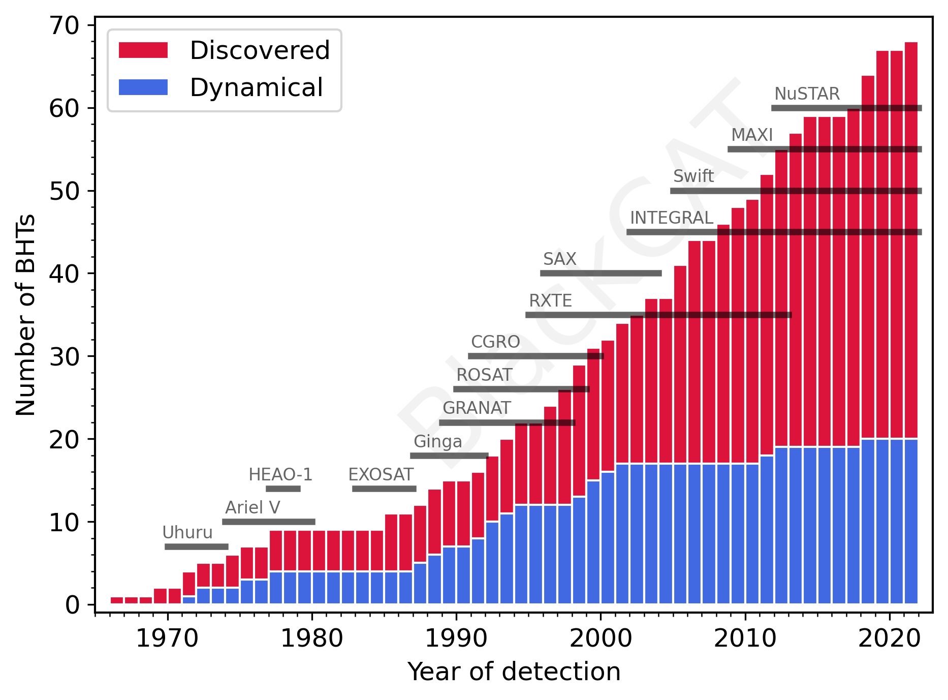
In 1972, it was found independently by Thomas Bolton Bolton (1972), and by Louise Webster and Paul Murdin Webster and Murdin (1972) that the X-ray source Cygnus X-1, discovered in 1964, had a massive stellar companion, and from its motion a first estimate for the mass of Cygnus X-1 was derived, exceeding the maximum mass of a NS and making it the first stellar black hole candidate. This finding helped to finally convince the scientific community of the existence of black holes in the Universe, and since then the set of known BHs has slowly grown, along with the set of known BH masses, in most cases still determined from the observation of X-ray sources. Along the way, a rich zoo of X-ray binaries has developed (see Figure 3 for the evolution of the number of discovered BH X-ray transients), followed by a diversification of the methods through which BHs can be detected. Besides X-ray binaries, BH masses have now also been constrained in non-interacting binaries, and for the first time from the microlensing of background light by a stellar black hole. Beyond the Galaxy, the GW measurements by LVK have since 2015 built up a catalog of compact object mergers that as of its latest iteration, the third GW Transient Catalog (GWTC-3) The LIGO Scientific Collaboration et al. (2021) contains 90 different events with well constrained masses, 83 of which are confirmed BH-BH mergers, totaling 166 confirmed extragalactic BH masses. Five BH-NS merger or merger candidates add another 5 masses to the sample.
This diversity, however, has also meant that the treatment of mass estimates has not always been consistent across the field, as credibility interval conventions have changed and the advent of Monte Carlo methods for dealing with distributed quantities has brought about an ease-of-use of the entire mass probability distribution, whatever its shape, and not just of central values and credibility intervals.
In this section, we build a regularized catalog of stellar BH masses and orbital parameters. For this, we have extensively searched the current literature and collected data both already present and not present in existing black hole catalogs (Corral-Santana et al., 2016; Tetarenko et al., 2016), resulting in a total of 35 objects for which we have recalculated all masses, where possible, based on a standardized method and Monte Carlo computations. In what follows, we first discuss the treatment of uncertainty when it comes to the mass estimates (Section 3.1), before briefly reviewing the nature of the observed systems (Section 3.2), introducing the standard mass computation procedure (Section 3.3) and presenting them system-by-system, along with some outstanding conflicts in their study (Section 3.4). In Section 3.5, we fit simple distributions to the entire mass sample, and make a first, simple, comparison of the resulting Galactic BH mass distribution to the extragalactic distribution from the LVK observations. Finally, in Section 3.6, we present a short overview of the current state of the lower mass gap problem in light of recent observations.
3.1 Treatment of Uncertainties
When probing reality, no measurement of continuous quantities is exact. With some degree of uncertainty always present, the best that can be hoped for is a probability distribution (rigorously, a probability density function, or PDF) for the actual value of each observable. More often than not, as a consequence of the central limit theorem, the resulting distribution is best described by a Gaussian, which, conveniently, is fully defined by its mean (equal to its mode), given as the observable’s nominal value; and its standard deviation , which measures the degree of certainty with which the observable’s actual value has been constrained.
Even though it is a very elegant way to describe data, representing the distribution of a physical quantity with only two values can distort the actual measurement, especially when uncertainties are large and the quantity of interest has been derived from other quantities with their own distributions. A problem that one finds when delving into the literature of compact objects is the lack of clarity in the definition of each measurement. Over many different authors and years of publication, definitions of the credibility ranges of reported results have not always been explicitly given, and nominal values as well are not clearly defined to report either the mean or mode of the corresponding distribution, which are the same only for unimodal symmetric distributions.
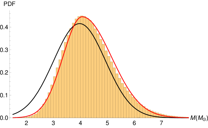
Dynamic mass measurements of black holes can be particularly vulnerable to this, as they are derived from the measurement of orbital parameters such as the period, velocity semi-amplitude of the companion and, of particular significance, the inclination of the orbital plane, on which mass estimates depend as , and which tends to make its uncertainties more asymmetric. Figure 4 shows the degree to which BH dynamic masses can deviate from a simple Gaussian due to a broad inclination range. This gives rise to the necessity of a more precise, yet still easily reproducible way of describing such quantities.
We therefore suggest and follow in this paper the practice of always providing any parameters of interest, whether directly observed or calculated, in the form of best-fit probability distributions of their value, so that a minimum of information is lost when using the data elsewhere. For simplicity, we will work with only three types of distribution: a uniform distribution, , between and ; a simple Gaussian distribution, , with mean and standard deviation ; and what we term an asymmetric Gaussian, , defined as
| (3) |
as a distribution over a variable , where m is the mode of the distribution (not equal to its mean), while and we call the superior and inferior "standard deviations". Formally, the parameter () is defined st. the probability of a random variable to be drawn from () is times the probability of to be drawn from (-).
We highlight that, in any case, the probability distribution for the mass of an individual BH is a reflection solely of current limitations in our knowledge of its related observable properties (orbital parameters, generally). Neither the asymmetric nor the simple Gaussian are taken as definite best-fits to the known distributions; as stated above, a simple Gaussian often results naturally to good approximation as a consequence of the central limit theorem. The proposed asymmetric Gaussian is the simplest extension of the symmetric distribution for observables with asymmetrical confidence intervals.
Equipped with these distributions, we examined all BHs with available mass measurements and carefully re-estimated their masses from known orbital parameters. We also included some well-constrained masses as they are reported, even if orbital parameters were not available, as discussed next.
3.2 Nature of Observations
As dark objects, and except in the case of GW signals from BH–BH mergers, BHs are observed exclusively by their interaction with other luminous sources, which in all but one existing detection means a binary companion. In some of these cases, transversal and radial velocity (RV) measurements from an observed star can be obtained and are enough to constrain the presence of a binary companion in order to explain the motion. If a massive companion is required, but none is observed, then it is most likely to be a BH. There have been so far three cases in which BH masses were measured in this manner for long-period giant star-black hole binaries, where only the giant is directly observed Liu et al. (2019); Thompson et al. (2019); El-Badry et al. (2022).
For closer binaries, however, another luminous source comes into play: accretion. Either by filling its Roche lobe or from stellar winds, the companion loses mass, part of which is captured by the compact component. As this matter falls toward it, it heats up from the conversion of gravitational potential energy and emits chiefly in the X-rays. Although these X-ray sources are collectively called X-ray Binaries (XRBs), they contain a large "zoo" of binary classes, starting from whether the compact object is an NS or a BH. In the following, we will briefly review some of the terminology and important observational methods for studying BHs in XRBs, but much of the discussion applies also to NS-hosting XRBs.
A first important distinction to be made among XRBs is whether accretion occurs through an accretion disk or not; the determining factor is if the specific angular moment of the infalling matter allows for direct impact onto the compact object. If matter loses energy but no angular momentum, then it would orbit at the circularization radius:
| (4) |
for an accretor of mass King (2006). Typically, disk formation occurs if the accretor’s effective radius is smaller than . For white dwarfs and NSs, the "effective radius" is equal to their radius if there is no significant magnetic field, but is of the order of the magnetospheric radius otherwise. For BHs, it is the radius of the innermost stable circular orbit (ISCO). As matter is accreted, both energy and angular momentum loss occur through viscosity. Once the above condition is fulfilled, disk formation occurs as energy is dissipated by viscosity and radiation faster than angular momentum is redistributed throughout the disk. The loss of energy drives the gas towards the lowest-energy orbit with its slowly-varying angular momentum, which is a circular one; thus, all the accreted gas settles into a series of concentric circular orbits, forming a disk. As gas keeps losing energy, the only way to fall to a lower energy orbit is by losing angular momentum, and in the absence of external torques, this occurs mainly by transferring momentum outward, causing the outer parts of the disk to spiral out Shakura and Sunyaev (1973); Shapiro et al. (1976). While this skips over many nuances of the process, the basic picture of the accretion disk is thus formed, as an efficient machine for lowering highly-rotating material onto the accretor, while converting the orbital energy into radiation, which we can observe.
The conditions above are nearly always fulfilled for Roche lobe overflow (RLOF), as the lost matter carries with it the specific angular momentum of the “parent”, and thus disk formation follows. Accretion from a stellar wind, on the other hand, becomes relevant for binaries with an O- or B-type companion in a close orbit, which is in fact the case for the first confirmed BH, Cygnus X-1. A simple calculation can tell us that in wind accretion the compact object captures only a fraction – of the mass lost by the companion, making it much less efficient than RLOF Frank et al. (2002). It is only because wind loss rates are so large (–) that these sources can still be observable. The winds, however, carry much less angular momentum, and thus do not necessarily lead to disk formation; the wind-fed pulsar Vela X-1, for example, has shown evidence of disk formation in the past Liao et al. (2020), but no such evidence has been observed so far in the known wind-fed BHs.
Most XRBs are observed in a quiescent state, in which their behavior broadly fits within the picture presented above. Occasionally, however, they are observed to undergo outbursts, during which their luminosity is greatly increased. For BH-hosting XRBs, the clearest examples are called soft X-ray transients (SXTs, which can also involve a NS instead), in which quiescence usually lasts for 1–50 yr with luminosities of , while outbursts last for weeks–months with a luminosity increase to Tauris and van den Heuvel (2006). The most common picture for explaining these outbursts is that of a disk instability (Frank et al., 2002), based on a distinction between two disk states: hot and high-viscosity (outburst); or cool and low-viscosity (quiescence). The state of the disk is determined essentially by the degree of hydrogen ionization, thus quiescence requires the absence of any ionization zones within the disk. This also defines the condition necessary for suppressing outbursts and making the system persistent: that the disk temperature always exceeds a characteristic hydrogen ionization temperature . Naturally, disks where is always true that would also be persistent, but very faint and lacking outbursts entirely; thus, if they exist, there is a strong bias against their detection King (2006). We refer the reader to the recent review by Hameury (2020) for a discussion of the disk instability model in the context of current problems.
The case where the disk temperature varies between being above or below brings us back to the SXTs. In this case, the outbursts are triggered by the formation of an ionization zone somewhere within the disk, which will be in the hot, viscous, state. This state of heightened energy dissipation favors an increased accretion rate onto the compact object, and thus an increased X-ray luminosity. The increased X-ray luminosity brings more and more of the disk into the hot state, increasing even more the rate of accretion, and so on. The heightened accretion tends to decrease the surface density of the gas, but the central X-ray irradiation stops this from effectively cooling the disk, which must remain trapped in the hot state until the accretion rate itself drops after a considerable accretion onto the compact object. This picture fits well with short-period SXTs, where the radius of the disk is limited, and it can become completely ionized during an outburst. Long-period SXTs, on the other hand, are able to comport much larger disks, a large portion of which can remain cold even during outbursts. The cold disk can act as a mass reservoir, making outbursts much longer than usual, to the point where some known persistent sources may actually be very long transients; a mass reservoir can also cause outbursts to occur in much quicker succession than expected. Disk warps also play a role, as they can affect the efficiency with which the X-ray source heats the full extent of the disk Tremaine and Davis (2014); Abarr and Krawczynski (2020). At the same time, a general “exhaustion” of the disk’s mass during long outbursts points towards very long quiescent periods as well, which implies a population of quiescent transients that have never been observed during an outburst (King, 2006).
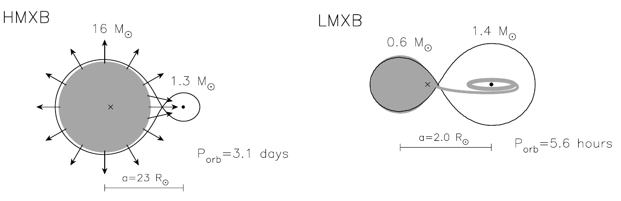
The discussion above leads naturally to the main distinction to be made among XRBs: low-mass X-ray binaries (LMXBs) and high-mass X-ray binaries (HMXBs). LMXBs are XRBs with luminous components with typical masses of or less, and so are restricted to RLOF accretion, which means that they virtually always contain an accretion disk (see the right side of Figure 5). Most, if not all, LMXBs are SXTs (King, 2006). We also see it fit to mention here that the phenomenon of X-ray bursts (and their associated binaries, the X-ray bursters) are entirely distinct from the disk outbursts. Type I X-ray bursts are thermonuclear in nature, similarly to novae, and can only occur in NS-hosting XRBs. For the less well understood Type II X-ray bursts, disk instability models have been proposed, but are not favored (see Bagnoli et al. (2015) for a review of some current proposals).
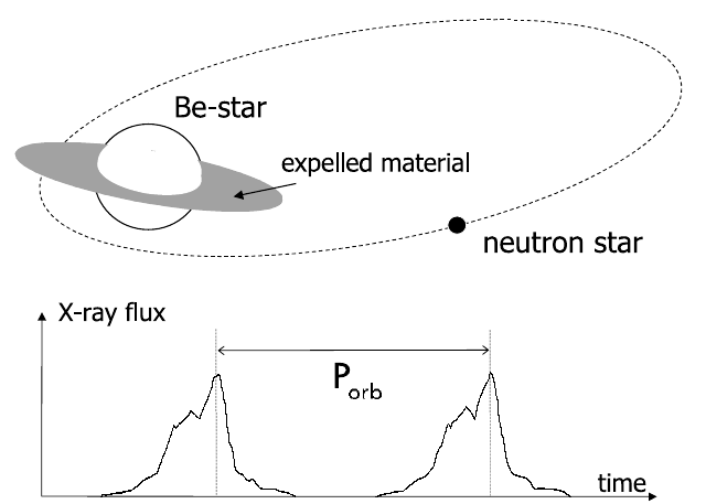
HMXBs contain massive companions (10 ) and generally undergo wind-fed accretion (see the left side of Figure 5), but can also accrete from RLOF, and form a disk. Even when they do have a disk, HMXBs rarely show disk instability outbursts because companion stars of type O or early B are themselves potent enough sources to keep the entire disk ionized (). Outbursts can then still occur if the components are distant enough during the orbit, i.e., if the period is longer than 10 d (Tauris and van den Heuvel, 2006), or for high-eccentricity orbits. These conditions are found in the particular class of Be X-ray binaries (Reig, 2011), in which the compact object accretes matter for the Be star’s own circumstellar disk; in this case, outbursts are regularly observed and probably caused by a burst of accretion near periastron (Figure 6). Although for some time only Be-NS binaries could be found, the first Be-BH binary was discovered in 2017 by Ribó et al. (2017).
Wind-fed HXMBs are generally persistent sources (classical HMXBs), with X-ray luminosities on the order of Lutovinov et al. (2013). However, a class of Supergiant Fast X-ray Transients (SFXTs) was discovered in 2005 (Sguera et al., 2005; Negueruela et al., 2006), which shows an average X-ray luminosity of , but bright X-ray flares lasting for a few days, composed of a series of bursts lasting for and with (Sidoli, 2017).
We can now point toward the sources for the majority of the mass estimates presented here. All but 4 of the 35 systems considered are XRBs; among them, 26 are LMXBs and 5 HMXBs. For all HMXBs and 22 of the LMXBs, we have recalculated the black hole mass from known orbital parameters , , , and, when available, . Observations of the luminous companion provides a powerful means to constrain the orbital period and companion velocity semi-ampitude . These constrain the mass function , which, together with the companion’s spectral type, constrains the mass ratio . For LMXBs, outburst observations are also available, although, for 4 of the LMXBs, only a mass estimate was available, which we adopted as given.
The inclination is harder to pin down. If an absence of eclipses is confirmed, an upper limit can be established from as indicated in the next section. If a disk is present, spectral methods for disk reflection can constrain . When jets are present (in this case, sometimes the system is called a microquasar (Corbel, 2011)), their inclination can be measured to a good degree of accuracy; however, it is not a safe assumption to take the jet inclination to be the same as the orbital inclination. In the general case of modeling the companion’s motion, detailed models can provide best-fit constraints on the inclination.
Indirect observation of BHs in non-interacting binaries can still occur through the monitoring of the companion’s motion, and the masses of three BHs in our sample have been constrained in this manner. Observation of isolated BHs is also possible from the microlensing of background light, but only one such event, which we have also included, has been confirmed so far to have been caused by a BH. Low-frequency Quasi Periodic Oscillations (LF QPOs) in the X-ray spectrum provide yet another way to measure the mass of a black hole in a XRB. QPOs appear in the power spectrum as narrow peaks and evolve through outbursts, with LF QPOs appearing with (for a review of QPOs and their different classes, see Ingram and Motta (2019)). XRB spectra can often be fitted by the superposition of a blackbody component and of a power law component (McClintock and Remillard, 2006), and Titarchuk and Fiorito (2004) produced a BH mass-dependent model which correlates the fitted photon index of the power-law component to the observed LF QPO frequency . This model has since also been used to measure the mass of XRBs in which LF QPOs are observed.
3.3 Mass Computation from Orbital Parameters
From all binaries, where available, we collect the orbital period and the velocity semi-amplitude of the companion to the BH. From these quantities, plus the eccentricity , the BH mass function is computed as
| (5) |
when considering a Keplerian orbit (Charles and Coe, 2006). The error incurred in the BH mass from assuming a Keplerian orbit is still much smaller than that from observational uncertainties in Keplerian parameters, in particular in the orbital inclination, which might be affected by serious systematic errors not yet taken into account in the present work (Kreidberg et al., 2012). We therefore employ Equation (5) as the relation between binary orbital parameters throughout the work.
In the following original sources for the LXMBs, we treat all systems as circularized, although a small but non-zero eccentricity might be allowed for them. For the HMXBs, eccentricities are reported, except for Gaia BH1, which was measured to have a modest . While for Gaia BH1, we consider its eccentricity in Equation (5), for all other systems we treat the orbit as circular. Once again, any incurred errors from this approximation are expected to be inferior to those from observational uncertainties and possible systematics not taken into account at present.
For each system, we also collect the binary inclination and the mass ratio . With these parameters, the BH mass can be determined as
| (6) |
We employ the above formula as a standardized computation of for all systems with orbital parameters, even when it results in a difference to the reported by the cited sources. In most cases where significant differences arise, they do so only as a broader range; and any considerable differences in the central value still keep the original mass within of ours. The orbital period is always an observed quantity, while is taken as an observed quantity in all but one case, in which it is computed from and . is in some cases taken as reported by the respective source, while, in others, it is computed from the source’s quoted and ; in two cases, we re-estimate it from the companion’s spectral type. The inclination is taken as reported from the sources. In all cases where the sources report a nominal value for a given quantity, that quantity is treated as an asymmetric Gaussian (Section 3.1) with mode at the nominal value; if the upper and lower uncertainties are reported, they are taken as and ; otherwise, these are set within of the mode. When only upper and lower bounds are reported, the quantity is taken as being distributed uniformly between them.
Whenever the inclination has not receive an upper limit while the mass ratio has been constrained, a lack of eclipses allows the determination of a maximum inclination from
| (7) |
Computations of Equations (5) and (6) are performed via Monte Carlo, and we fit our results to an asymmetric Gaussian, which in some cases results in a symmetric distribution regardless. The orbital parameters and resulting mass distributions are reported in Tables 2 and 3. Below, we offer a case-by-case, non-exhaustive, discussion of the objects reported in Table 3 and their references, under the considerations made in Section 3.1. We report the results as given by the references; in some cases, the mass ratio is reported as , or the masses , themselves are given. In those cases, we use MC to convert their distributions to a distribution of , unless stated otherwise.
3.4 Collected Systems
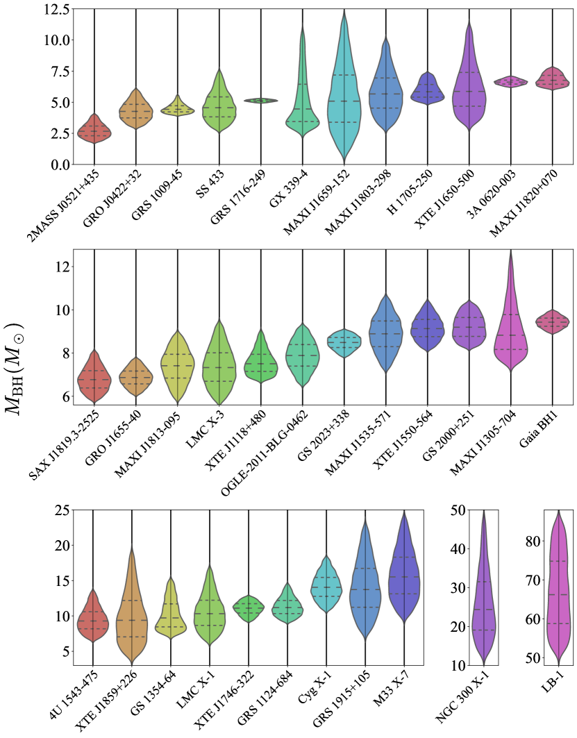
We present below the full catalog of BH mass measurements from 26 LMXBs, 5 HMXBs, 3 non-interacting binaries and 1 isolated BH. We discuss each object in turn, briefly indicating the manner of measurement, the original results we have adopted for our catalog, and conflicts found during their collection. The full sample is displayed in Table 3 with sources, our standardized mass determination and all orbital parameters except for the eccentricity, which was only explicitly available for six systems; for those we display, the eccentricity in Table 2. We show in Figure 7 the resulting mass distributions for all 35 BHs.
| Name | References | |
|---|---|---|
| Cyg X-1 | Orosz et al. (2011) | |
| LMC X-1 | Orosz et al. (2009) | |
| M33 X-7 | Orosz et al. (2007) | |
| SS 433 | Cherepashchuk (2022) | |
| LB-1 comp. | Liu et al. (2019) | |
| 2MASS J05215658+4359220 comp. | Thompson et al. (2019) | |
| Gaia BH1 | El-Badry et al. (2022) |
Eccentricities for the seven objects for which they were given, alongside the reference. is a normal distribution with mean and standard deviation , as defined in Section 3.1.
3.4.1 LMXBs
Sources with orbital parameters
We list here the 22 LMXBs for which the necessary orbital parameters for the procedure described in Section 3.3 were available.
4U 1453-475
Orosz (2003) compile an inventory of reliable BH-hosting binaries at the time of writing and their relevant parameters. We adopted their reported and . We convert their – range to a uniform distribution. We work backwards to compute from their and .
GRS 1915+105
Greiner et al. (2001) use spectroscopic data to measure and . The authors report that the jet angle determination of has been observed to be stable over several years, so that it is reasonable to assume it as the orbital plane inclination . With this inclination and a companion mass estimate of , they find . We adopt their , and , and compute from their estimates.
GS 1354-64
Casares et al. (2009) present a refined treatment of GS 1354-64 (BW Cir) in relation to the first evidence of the presence of a BH presented in Casares et al. (2004), and with spectroscopic and photometric data find , and , which we adopt. They report only an upper limit of for the inclination, so we adopt from Farr et al. (2011).
GRS 1124-684
Wu et al. (2015) present a study of optical spectroscopic and photometric data of GRS 1124-683 (Nova Muscae 1991), and from the radial velocity of the companion are able to determine , and , which we adopt. We adopt the inclination from their following study of the object (Wu et al., 2016), in which they constrain it to .
XTE J1118+480
González Hernández et al. (2014) use NIR spectroscopic data of XTE J1118+480 to measure , yielding values compatible with Torres et al. (2004); González Hernández et al. (2012); and , also compatible with previous work (Hernández et al., 2008). We adopt their results, and their quoted (Calvelo et al., 2009) and (Khargharia et al., 2012) from previous works.
3A 0620-003
González Hernández et al. (2014) recalculate the orbital period derivative for 3A 0620-003 with new spectroscopic data from Hernández and Casares (2010) and obtain a more precise value of for the period, which is compatible with previous work (McClintock and Remillard, 1986). We adopt their quoted , (Neilsen et al., 2008) and (Cantrell et al., 2010).
GS 2000+251
MAXI J1659-152
Torres et al. (2021) use spectroscopic data of the MAXI J1659-152 X-ray transient’s quiescent counterpart to constrain its orbital properties and confirm the compact object’s BH nature. We adopt their and . We adopt their report lower and upper limits for the mass ratio and inclination as distributions and , respectively.
MAXI J1305-704
Mata Sánchez et al. (2021) present photometric and spectroscopic data of the quiescent state of MAXI J1305-704 to confirm the presence of a BH in the binary. We adopt their determined and . For the mass ratio, the authors adopt a distribution truncated to . We adapt this distribution to an asymmetric normal by keeping the central value at and considering its distance to the truncation limits as , resulting in a distribution . We keep the authors’ favored inclination model, .
GS 2023+338
Casares and Charles (1994) use spectroscopic data to constrain the system parameters of GS 2023+338. We adopt from their Table 2 , and . Based on the parameters from Casares and Charles (1994); Khargharia et al. (2010), use new NIR spectroscopic data of GS 2023+338 to measure the inclination of the system as , which we adopt.
XTE J1650-500
Orosz et al. (2004) use R-band photometric data from XTE J1650-500 and confirm an orbital period . Reanalysis of archival spectroscopic data yields the velocity semi-amplitude . From the light curve, the authors find an inclination lower limit of and report an upper lower limit of from the absence of eclipses. Although the exact upper limit depends on the mass ratio, we adopt a distribution for . The mass ratio can be measured from the companion’s spectral type, but due to the small amount of template spectra available, cannot be well-constrained. From the sample available, the best match is reported to be K4 V, from which we derive a conservative distribution of for .
GRO J0422+32
Webb et al. (2000) use photometric and spectroscopic data of GRO J0422+32 to model the binary. We adopt their measured and , and also the derived . They constrain the mass of the compact object to >, at that point still allowing for a massive NS. Ref. Gelino and Harrison (2003) studied new optical and IR photometric data of the X-ray transient and were able to show that it should contain a light BH, not an NS. They measure the most likely value for the inclination as , which corresponds to a most likely . While Webb et al. (2000) find M4 V as the best-matching spectral type for the companion, Ref. Gelino and Harrison (2003) arrive at M1 V; they argue that an M4 V type cannot be made compatible with the observations unless an extra source of blue luminosity is posited, but that this source is also incompatible with observations.
H 1705-250
Remillard et al. (1996) use photometric and spectroscopic data of H 1705-250 (Nova Ophiuchi 1977) to support the presence of a BH in the system and measure and . The companion’s spectrum is best matched by a type K5, yielding , which we adopt.
Harlaftis et al. (1997) use spectroscopic data from Keck to model H 1705-250 and fit also a K5 spectrum to the companion. They constrain the inclination to , and we adopt this result as a distribution .
GRO J1655-40
Hernández et al. (2008) use new optical and UV, as well as archival NIR, spectrographic data to study GRO J1655-40 (Nova Scorpii 1994) with the main goal of performing an abundance analysis of its secondary. They provided updated measurements of the orbital parameters which we adopt: , and . For the inclination, they adopt from Beer and Podsiadlowski (2002), and so we also adopt this result.
The authors suggest that the found by Shahbaz (2003) might be more accurate by virtue of having incorporated the secondary’s Roche geometry in their spectral analysis. However, Shahbaz (2003) use from Greene et al. (2001) in their study. We choose to keep both the and from Hernández et al. (2008) for consistency.
XTE J1859+226
Corral-Santana et al. (2011) use spectroscopic and photometric data of XTE J1859+226 and find from the secondary’s motion and , which we adopt. These values imply a mass function , in considerable excess of the previously reported (Filippenko and Chornock, 2001), but we note that the older result has only been presented in an IAU Circular and has been considered unreliable (Özel et al., 2010). The authors also report a best-match K5 V for the companion’s spectral type, and we set for a distribution .
The absence of eclipses imposes an upper limit on the inclination, but the available data are considered not accurate enough to properly estimate the inclination angle. By assuming a secondary similar to that of 3A 0620-00 and the known orbital parameters, the authors arrive at a preferred range . We thus adopt for the inclination a distribution .
MAXI J1803-298
Sánchez et al. (2022) use optical photometric data taken during the discovery outburst of MAXI J1803-298 to model the binary and provide evidence supporting the compact object’s BH nature. Its orbital period has so far only been measured as , so we adopt a distribution. The authors are able to constrain the companion’s velocity semi-amplitude to a 460–570 (410–620) () confidence interval, so we take as our distribution. For the mass ratio, they assume a typical range, which we take as a distribution. The authors report a > lower inclination limit but no upper limit; as no eclipses are reported, we compute an upper limit of and take as the distribution.
MAXI J1820+070
Torres et al. (2019) confirm the presence of a BH in the X-ray binary MAXI J1820+070 with spectroscopy from its decline to the quiescent state, and we adopt their and . Ref. Torres et al. (2020) use optical spectroscopy of the object to further constrain the mass ratio to and the inclination to , both of which we adopt, the inclination as .
XTE J1550-564
Orosz et al. (2011) fit optical and NIR spectroscopic and photometric data from observations of XTE J1550-564 to a set of eight lightcurve models. Although the authors point out that there are conflicts between data taken at different times, we adopt their nominal result , and ; and, from their , we adopt . Ref. Connors et al. (2020) reports an inclination estimate of which is inconsistent with the older estimate. They conclude that it may be the case that this object has a warped disk, or that the disk structure may be obscuring blueward line emission, resulting in lower inclination estimates from reflection modeling.
GX 339-4
Heida et al. (2017) measure the donor star RV curve with data from VLT/X-shooter, chiefly NIR and optical, from which they obtain and , which is significantly lower than the previous lower limit of (Hynes et al., 2003), leading also to a lower than previously reported. The authors argue that the scenario in which their is underestimated would imply variations of the absorption lines of the donor along the orbit, while their data cover most orbital phases and shows no such variations, which, among other factors, expanded upon in the cited work, support their measured .
From their , Heida et al. (2017) find and a lower limit for the inclination of . We adopt the quoted upper limit of derived from the absence of eclipses and treat the inclination distribution as . We adopt their nominal results for and .
GRS 1009-45
Filippenko et al. (1999) employ optical spectra from GRS 1009-45 (Nova Velorum 1993) during quiescence and measure and from the companion’s RV curve. Approximate radial velocities of the compact primary from the H emission line allow for a mass ratio determination and inclination . We adopt their results for , and , and by our standard treatment assume that the inclination is distributed as . We highlight that the lack of eclipses imposes a limit on inclination, but because the mass depends on only, which varies minimally for , we keep as our distribution for simplicity.
Macias et al. (2011) have reported refined measurements of and for this system. We, however, do not employ these results here as they are only available in the form of an abstract, and the cited source provides neither nor .
LMC X-3
With a companion of about , LMC X-3 does not fit neatly into the LMXB / HMXB dichotomy we have described before; it can be placed instead in the small class of intermediate-mass XRBs, which suffer from a negative selection bias (see Tauris and van den Heuvel (2006)). Orosz et al. (2014) study a large set of new and archival spectroscopic and photometric data to model LMC X-3. We employ the “Adopted value” for the parameters from the X-ray heating model in their Table 10, and . and are taken as quoted. Their resulting is considerably different from older estimates but is deemed more reliable as it derives from a much larger body of observations, and was obtained after measuring and taking into account for the first time the rotation of the secondary. The authors include a brief review of previous results and discuss the sources of inconsistencies.
SAX J1819.3-2525
From spectroscopic observations of SAX J1819.3-2525 (V4641 Sgr), Orosz et al. (2001) confirm the BH nature of the system’s compact object and measure and , which we adopt. MacDonald et al. (2014) gather of photometric data from the system and are able to measure and , which we adopt. Although their estimated distance () is below that of Orosz et al. (2001) (), their and were derived by fixing the same orbital period and a compatible (Lindstrøm et al., 2005), and so we consider the parameters to be compatible. With the companion mass estimate as () by Orosz et al. (2001), this system is also an IMXB candidate.
Sources with mass estimate only
For another four LMXBs, mass estimates were available, but not their orbital parameters. Although this means that, for these objects, we cannot perform the standardized mass computation from Section 3.3, we still include their masses in our sample. We treat them as symmetric or asymmetric Gaussians and their reported uncertainties as unless stated otherwise by the sources. The systems here included are: GRS J1716-249, MAXI J1813-095, MAXI J1535-571, and XTE J1746-322.
GRS J1716-249
Zhang et al. (2022) study X-ray spectroscopic data from the 2016–2017 outburst of binary GRS J1716-249 with continuum-fitting and ironline methods, with the aim of testing the Kerr nature of the system’s BH. For their preferred result of assuming an exact Kerr metric, they find , and within the same model constrain the inclination to . We include both results in our sample.
MAXI J1813-095
Jana et al. (2021) perform timing and spectral analyses of the 2018 outburst of binary MAXI J1813-095. They consider three sets of observational data and obtain a mass estimate from each one. We include as a mass estimate the average result, (). They also place constraints on the inclination, which we adopt as a distribution .
MAXI J1535-571
Shang et al. (2019) perform timing and spectral analysis of data from its 2017–2018 outburst. From their spectral analysis, they find the mass range 7.9–9.9, and we include in our sample their suggested mass .
XTE J1746-322
Spectral studies of the microquasar XTE J1746-322 (H 1743-322) have been performed recently by Molla et al. (2017) and Tursunov and Kološ (2018). Molla et al. (2017) perform timing and spectral analyses on observations from two outbursts, in 2010 and 2011, from which they estimate a mass range –. They also study observed QPOs during the outburst, from which a second mass estimate is derived, . By combining the two results, they arrive at , which we include in our sample. Notably, Tursunov and Kološ (2018) employ a different method to also study the QPOs observed in this object and arrive at a mass estimate of .
3.4.2 HMXBs
We list here the five HMXBs with mass estimates, all of which include the necessary orbital parameters for the procedure described in Section 3.3.
Cyg X-1
Orosz et al. (2011) use an improved distance measurement for Cyg X-1 together with previously published optical data to model the system. The period is fixed to from Brocksopp et al. (1999) and the data are fitted to four models. We adopt the fixed period and the final parameters from Table 2: , , and . We compute with MC from and . We adopt their more scattered fitted to the data from Gies et al. (2003).
LMC X-1
Orosz et al. (2009) use optical spectroscopic, and optical and NIR photometric, data to model LMC X-1 and confirm earlier work by Hutchings et al. (1987) with much higher precision. We employ the “Adopted Value” from their Table 3 for , , , and . We also report their resulting from their "Eccentric Orbit" values in Table 3.
M33 X-7
NGC 300 X-1
Crowther et al. (2010) confirmed the nature of system NGC 300 X-1 as a Wolf–Rayet/black hole binary located in the Sculptor group galaxy NGC 300 (). They use optical spectroscopic data and determine and , of which we adopt the latter. For the period, we adopt the more recent from Binder et al. (2021), where new X-ray and UV observations are combined with archival X-ray observations to further constrain the binary model. We adopt their mass estimate of for the WR companion and to recover the distribution; these estimates are consistent with , so we adopt a distribution for the inclination.
SS 433
Discovered in the 1970s, SS 433 is the first observed Galactic microquasar, today generally agreed on to be an eclipsing X-ray binary undergoing supercritical accretion onto the compact object. Over the more than 40 years during which this object has been studied, considerably different estimates of the component masses have been put forward. We have taken our parameters for this system from the recent review by Cherepashchuk (2022), which reports results from the over 40 years of observations of SS433 in the optical, radio, and X-rays. We adopt the quoted nominal value for the orbital period from the review and assign it a conservative uncertainty in the last digit, yielding . The inclination is given as , so we adopt the distribution . We also collected the measured eccentricity of .
For the velocity semi-amplitude, we adopt the reported from Picchi et al. (2020), and, for consistency, also adopt the mass estimates from that same work, and , which result in a mass ratio .
A more recent estimate by Cherepashchuk et al. (2021), however, has led to a lower limit of which implies a relatively massive BH with . We do not adopt this result presently as it does not provide the parameters necessary for our standardized mass computation.
3.4.3 Other Sources
In addition to the X-ray binaries, we have collected four recent BH observations with mass and, where applicable, orbital parameter measurements, which we detail here. These are the three non-interacting binaries, LB-1, 2MASS J05215658+4359220 (J0521+435) and Gaia BH1; and the microlensing event OGLE-2011-BLG-0462.
LB-1 comp.
Liu et al. (2019) report the results from over two years of radial-velocity measurements of the Galactic B-type star LB-1 (LS V +22 25) and find that its motion requires the presence of a () BH in a orbit. From the best-fit model for the H emission line, they also find and , and, from the companion’s spectra, they find . We adopt these values for the object.
2MASS J0521+435 comp.
Thompson et al. (2019) study spectroscopic and photometric data from the giant star J0521+435 and determine that it must be in a , and orbit with and an unseen BH companion. By comparing the giant’s properties to single-star evolutionary models, they find for the inclination and for the masses (). We adopt these nominal results for the object, although the authors also employ other methods that arrive at different but compatible estimates; the unseen companion’s mass is consistently estimated to be in the 2.9– range, which keeps it a likely low-mass black hole.
Gaia BH1
El-Badry et al. (2022) study a a bright solar-type star in Ophiuchus with astrometric data from the Gaia mission and follow-up spectroscopy, and determine from the Gaia orbital solution and RV measurements that the star must orbiting an unseen companion. We adopted the quoted mass for the solar-type companion, and their results derived from astrometric and RV data: , , and . We adopt the derived from RV data only. This is the only confirmed BH binary with a modest but non-negligible eccentricity, as well as the closest known BH, at the moment of writing, and potentially originated from either a triple system or dynamical assembly.
| \PreserveBackslash Name | \PreserveBackslash | \PreserveBackslash | \PreserveBackslash | \PreserveBackslash | \PreserveBackslash | \PreserveBackslash | \PreserveBackslash References |
| \PreserveBackslash | \PreserveBackslash day | \PreserveBackslash km s-1 | \PreserveBackslash | \PreserveBackslash deg | \PreserveBackslash | \PreserveBackslash | \PreserveBackslash |
| \PreserveBackslash 4U 1543-475 | \PreserveBackslash | \PreserveBackslash | \PreserveBackslash | \PreserveBackslash | \PreserveBackslash | \PreserveBackslash | \PreserveBackslash Orosz (2003) |
| \PreserveBackslash GRS 1915+105 | \PreserveBackslash | \PreserveBackslash | \PreserveBackslash | \PreserveBackslash | \PreserveBackslash | \PreserveBackslash | \PreserveBackslash Greiner et al. (2001) |
| \PreserveBackslash GS 1354-64 | \PreserveBackslash | \PreserveBackslash | \PreserveBackslash | \PreserveBackslash | \PreserveBackslash | \PreserveBackslash | \PreserveBackslash Casares et al. (2009); Farr et al. (2011) |
| \PreserveBackslash GRS 1124-684 | \PreserveBackslash | \PreserveBackslash | \PreserveBackslash | \PreserveBackslash | \PreserveBackslash | \PreserveBackslash | \PreserveBackslash Wu et al. (2015, 2016) |
| \PreserveBackslash XTE J1118+480 | \PreserveBackslash | \PreserveBackslash | \PreserveBackslash | \PreserveBackslash | \PreserveBackslash | \PreserveBackslash | \PreserveBackslash González Hernández et al. (2014) |
| \PreserveBackslash 3A 0620-003 | \PreserveBackslash | \PreserveBackslash | \PreserveBackslash | \PreserveBackslash | \PreserveBackslash | \PreserveBackslash | \PreserveBackslash González Hernández et al. (2014) |
| \PreserveBackslash GS 2000+251 | \PreserveBackslash | \PreserveBackslash | \PreserveBackslash | \PreserveBackslash | \PreserveBackslash | \PreserveBackslash | \PreserveBackslash Ioannou et al. (2004) |
| \PreserveBackslash MAXI J1659-152 | \PreserveBackslash | \PreserveBackslash | \PreserveBackslash | \PreserveBackslash | \PreserveBackslash | \PreserveBackslash | \PreserveBackslash Torres et al. (2021) |
| \PreserveBackslash MAXI J1305-704 | \PreserveBackslash | \PreserveBackslash | \PreserveBackslash | \PreserveBackslash | \PreserveBackslash | \PreserveBackslash | \PreserveBackslash Mata Sánchez et al. (2021) |
| \PreserveBackslash GS 2023+338 | \PreserveBackslash | \PreserveBackslash | \PreserveBackslash | \PreserveBackslash | \PreserveBackslash | \PreserveBackslash | \PreserveBackslash Casares and Charles (1994); Khargharia et al. (2010) |
| \PreserveBackslash XTE J1650-500 | \PreserveBackslash | \PreserveBackslash | \PreserveBackslash | \PreserveBackslash | \PreserveBackslash | \PreserveBackslash | \PreserveBackslash Orosz et al. (2004) |
| \PreserveBackslash GRO J0422+32 | \PreserveBackslash | \PreserveBackslash | \PreserveBackslash | \PreserveBackslash | \PreserveBackslash | \PreserveBackslash | \PreserveBackslash Webb et al. (2000); Gelino and Harrison (2003) |
| \PreserveBackslash H 1705-250 | \PreserveBackslash | \PreserveBackslash | \PreserveBackslash | \PreserveBackslash | \PreserveBackslash | \PreserveBackslash | \PreserveBackslash Harlaftis et al. (1997); Remillard et al. (1996) |
| \PreserveBackslash GRO J1655-40 | \PreserveBackslash | \PreserveBackslash | \PreserveBackslash | \PreserveBackslash | \PreserveBackslash | \PreserveBackslash | \PreserveBackslash Hernández et al. (2008); Beer and Podsiadlowski (2002) |
| \PreserveBackslash XTE J1859+226 | \PreserveBackslash | \PreserveBackslash | \PreserveBackslash | \PreserveBackslash | \PreserveBackslash | \PreserveBackslash | \PreserveBackslash Corral-Santana et al. (2011); Kreidberg et al. (2012) |
| \PreserveBackslash MAXI J1803-298 | \PreserveBackslash | \PreserveBackslash | \PreserveBackslash | \PreserveBackslash | \PreserveBackslash | \PreserveBackslash | \PreserveBackslash Mata Sánchez et al. (2021) |
| \PreserveBackslash MAXI J1820+070 | \PreserveBackslash | \PreserveBackslash | \PreserveBackslash | \PreserveBackslash | \PreserveBackslash | \PreserveBackslash | \PreserveBackslash Torres et al. (2019, 2020) |
| \PreserveBackslash XTE J1550-564 | \PreserveBackslash | \PreserveBackslash | \PreserveBackslash | \PreserveBackslash | \PreserveBackslash | \PreserveBackslash | \PreserveBackslash Orosz et al. (2011) |
| \PreserveBackslash GX 339-4 | \PreserveBackslash | \PreserveBackslash | \PreserveBackslash | \PreserveBackslash | \PreserveBackslash | \PreserveBackslash | \PreserveBackslash Heida et al. (2017) |
| \PreserveBackslash GRS 1009-45 | \PreserveBackslash | \PreserveBackslash | \PreserveBackslash | \PreserveBackslash | \PreserveBackslash | \PreserveBackslash | \PreserveBackslash Filippenko et al. (1999) |
| \PreserveBackslash LMC X-3 | \PreserveBackslash | \PreserveBackslash | \PreserveBackslash | \PreserveBackslash | \PreserveBackslash | \PreserveBackslash | \PreserveBackslash Orosz et al. (2014) |
| \PreserveBackslash SAX J1819.3-2525 | \PreserveBackslash | \PreserveBackslash | \PreserveBackslash | \PreserveBackslash | \PreserveBackslash | \PreserveBackslash | \PreserveBackslash MacDonald et al. (2014); Orosz et al. (2001) |
| \PreserveBackslash GRS 1716-249 | \PreserveBackslash - | \PreserveBackslash - | \PreserveBackslash - | \PreserveBackslash | \PreserveBackslash - | \PreserveBackslash | \PreserveBackslash Zhang et al. (2022) |
| \PreserveBackslash MAXI J1813-095 | \PreserveBackslash - | \PreserveBackslash - | \PreserveBackslash - | \PreserveBackslash | \PreserveBackslash - | \PreserveBackslash | \PreserveBackslash Jana et al. (2021) |
| \PreserveBackslash MAXI J1535-571 | \PreserveBackslash - | \PreserveBackslash - | \PreserveBackslash - | \PreserveBackslash - | \PreserveBackslash - | \PreserveBackslash | \PreserveBackslash Shang et al. (2019) |
| \PreserveBackslash XTE J1746-322 | \PreserveBackslash - | \PreserveBackslash - | \PreserveBackslash - | \PreserveBackslash - | \PreserveBackslash - | \PreserveBackslash | \PreserveBackslash Molla et al. (2017) |
| \PreserveBackslash Cyg X-1 | \PreserveBackslash | \PreserveBackslash | \PreserveBackslash | \PreserveBackslash | \PreserveBackslash | \PreserveBackslash | \PreserveBackslash Brocksopp et al. (1999); Orosz et al. (2011) |
| \PreserveBackslash LMC X-1 | \PreserveBackslash | \PreserveBackslash | \PreserveBackslash | \PreserveBackslash | \PreserveBackslash | \PreserveBackslash | \PreserveBackslash Orosz et al. (2009) |
| \PreserveBackslash M33 X-7 | \PreserveBackslash | \PreserveBackslash | \PreserveBackslash | \PreserveBackslash | \PreserveBackslash | \PreserveBackslash | \PreserveBackslash Pietsch et al. (2006); Orosz et al. (2007) |
| \PreserveBackslash NGC 300 X-1 | \PreserveBackslash | \PreserveBackslash | \PreserveBackslash | \PreserveBackslash | \PreserveBackslash | \PreserveBackslash | \PreserveBackslash Binder et al. (2021); Crowther et al. (2010) |
| \PreserveBackslash SS 433 | \PreserveBackslash | \PreserveBackslash | \PreserveBackslash | \PreserveBackslash | \PreserveBackslash | \PreserveBackslash | \PreserveBackslash Cherepashchuk (2022); Picchi et al. (2020) |
| \PreserveBackslash LB-1 cp. | \PreserveBackslash | \PreserveBackslash | \PreserveBackslash | \PreserveBackslash | \PreserveBackslash | \PreserveBackslash | \PreserveBackslash Liu et al. (2019) |
| \PreserveBackslash 2MASS J0521+435 cp. | \PreserveBackslash | \PreserveBackslash | \PreserveBackslash | \PreserveBackslash | \PreserveBackslash | \PreserveBackslash | \PreserveBackslash Thompson et al. (2019) |
| \PreserveBackslash Gaia BH1 | \PreserveBackslash | \PreserveBackslash | \PreserveBackslash | \PreserveBackslash | \PreserveBackslash | \PreserveBackslash | \PreserveBackslash El-Badry et al. (2022) |
| \PreserveBackslash OGLE-2011-BLG-0462 | \PreserveBackslash - | \PreserveBackslash - | \PreserveBackslash - | \PreserveBackslash - | \PreserveBackslash - | \PreserveBackslash | \PreserveBackslash Mróz et al. (2022) |
In each line, we identify the name of the source containing the black hole, as well the BH mass and available orbital parameters; when these are available, the indicated BH mass is the result of our standardized calculation (Section 3.3); otherwise, it corresponds to the nominal result from the references. For the systems with more than one source, which parameters where taken from which source are specified in Section 3.4. The distributions are given in terms of the notation established in Section 3.1: indicates a normal distribution with mean and standard deviation , while an asymmetrical normal distribution with mode , standard deviation above and standard deviation below. indicates a uniform distribution between and .
OGLE-2011-BLG-0462
The microlensing event OGLE-2011-BLG-046S (OB110462) marks the first discovery an isolated BH. It was made independently by Lam et al. (2022) with data from the Optical Gravitational Lensing Experiment (OGLE), and by Sahu et al. (2022) with data from the Microlensing Observations in Astrophysics (MOA) survey, with initially conflicting mass estimates of 1.6– and , respectively. A simultaneous re-analysis of all available data from OB110462 by Mróz et al. (2022) later confirmed a mass of for the object, which we include in our sample.
3.5 The Full Mass Distribution
One of the great interests in building an updated and standardized catalog of BH masses is to verify the shape of the full Galactic BH mass distribution and to match it to analytical models, which may be made available for use in further work concerning BH populations. Özel et al. (2010) and Farr et al. (2011) performed the last such modeling more than 10 years ago, with samples of 16 and 20 BHs, respectively. At that time, through Bayesian methods, they found that, for a simple Gaussian, the preferred distribution had a mean and standard deviation . On the other hand, Farr et al. (2011) also considered a double Gaussian model, and found for it a Bayesian evidence greater than that for the simple Gaussian. We present here a simple goodness-of-fit test for an asymmetric Gaussian model to our full sample and compare it to the previous results. A full investigation of the mass distribution with more robust methods and including further corrections for systematics and biases (Kreidberg et al., 2012; Jonker et al., 2021) will be developed in a future work (Bernardo et al., in preparation).
From each of the 35 mass distributions in Table 3, we draw masses, and fit an asymmetric Gaussian to the mixture of these draws, resulting in , and . The sample histogram is displayed along with the asymmetric Gaussian fit in Figure 8. The mode of the distribution (m) results in a value not too distinct to the result from Özel et al. (2010) for a sample two times smaller, indicating the robustness of a peak in this region, while allowing for asymmetry, leads to quite different .
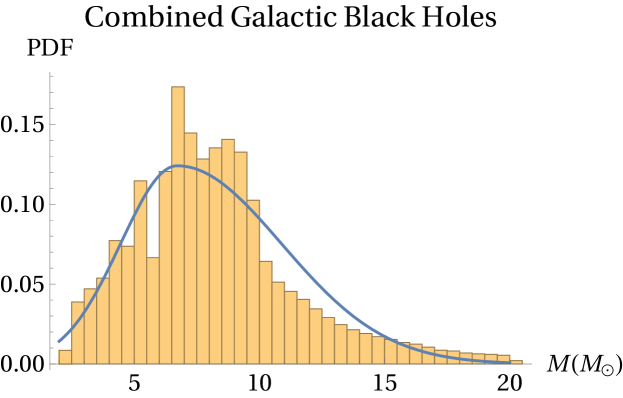
While a full analysis of the currently known extragalactic BH masses measured by LVK is out of the scope of this work, some first considerations and a simple comparison stand to be made. It must first be highlighted that there is no simple way to derive a single distribution from both Galactic and extragalactic samples simultaneously, as not only are they affected by different observational biases, but also the underlying physical distribution itself is not necessarily the same. Different environmental conditions at the higher redshifts probed by GW observations could change the shape of the distribution by affecting the process of stellar and binary evolution. Lower metallicites, for example, make wind mass loss from giant stars less efficient (e.g., Pols et al. (1998)), while both low metallicities and high star formation rates have been linked to a top-heavy initial mass function (see the reviews by Kroupa et al. (2013); Hopkins (2018)), which could be expected to lead to a BH mass distribution shifted to higher masses.
With that in mind, we have collected the raw BH mass distributions made available by LVK (Monte Carlo samples of masses for each object) as part of GWTC-3 The LIGO Scientific Collaboration et al. (2021) and produced their mixture distribution with no further processing of the data. Unlike the Galactic distribution, the extragalactic distribution shows two peaks, which we fitted to a double Gaussian in order to determine the location and breadth of each one. Figure 9 shows the resulting fit, with a lower peak , , with weight ; and an upper peak , . Even though a direct comparison cannot be directly made, as discussed, it is still noteworthy that a lower peak from the GW sources seems to align with the single Galactic peak as shown in Figure 10. This lower peak is mainly caused by the new additions to GWTC-3 in relation to GWTC-2 The LIGO Scientific Collaboration et al. (2021). It may then be connected to the improvements in sensitivity made to the observatories between each new run, which allow for the detection of lower-mass sources than in previous runs. Although a safe conclusion may only be derived after a careful modeling and consideration of observational biases for both samples, this might lend credence to the idea that a Galactic-like population of BHs exists in galaxies at higher redshift (1).
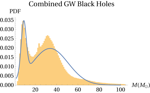
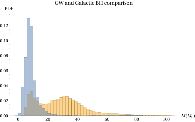
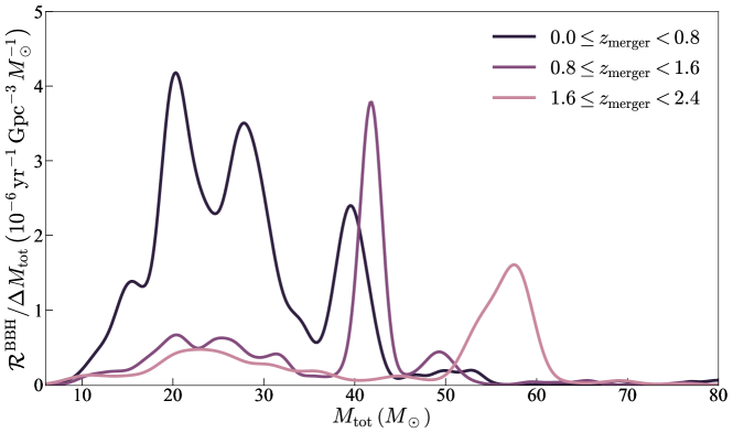
On the other hand, the GW mass distribution shows a high-mass peak which is entirely absent from the Galactic distribution. Although it is hard to treat the existing Galactic BH sample as reflective of the real mass distribution with its current size, this also might indicate that high-redshift populations allow for the production of more massive BHs than local populations. If mass-redshift correlations are present in the GW sample, then they might support the aforementioned idea that low-metallicity and high-star formation rate conditions at high redshift lead to the birth of more massive stars, Chruślińska et al. (2020) which in turn allow for an increased production of more massive BHs, and consequently of more massive BH mergers, as has been indicated by population synthesis studies that consider environment-dependent initial mass functions and star formation rates ((Neijssel et al., 2019; de Sá et al., ), see also Figure 11) and tentatively supported by GW observations Fishbach et al. (2021). A full consideration will, however, still require accounting for observational biases and for a study of the redshift distribution in GWTC-3 and future catalogs.
3.6 The Lower Mass Gap
We note from Figures 8 and 9 that both the Galactic and extragalactic mass distributions smoothly extend into the < region to a significant level; in fact, six of our objects — MAXI J1659152, GRO J0422+32, GX 3394, GRS 100945, SS 433 and 2MASS J0521+435 cp. — all have mass distributions with central values below . This makes them candidates for being within the – lower mass gap in the BH mass distribution, an apparently empty mass range above the maximum NS mass first indicated by Bailyn et al. (1998) from a sample of seven LMXBs. With their expanded samples of XRBs, Özel et al. (2010) in 2010 and Farr et al. (2011) in 2011 still found evidence for a gap in the BH mass distribution below , and so its existence has remained an open question for over 20 years. The gap has been connected to the characteristic convection timescale in core-collapse supernovae (Fryer et al., 2012; Belczynski et al., 2012), but even in this case a partial filling has not been ruled out. Ongoing work on this issue (Fryer et al., 2022; Olejak et al., 2022) can now be taken both ways, as while in one hand an appropriate convection timescale can help explain the existence of the gap, a measure of the gap depth can help constrain the convection timescale. Other mechanisms for compact object production, such as AIC in WD binaries and accretion in "spider" binaries, have also been suggested to fill the gap to some extent Horvath et al. (2022), but the hypothesis of a partially filled gap has remained mostly speculative until recently.
Objects such as the six we mention from our sample, as well as light BHs detected by LVK have in the past few years started to offer observational support for the partial gap hypothesis. Farah et al. (2022) performed a Bayesian study of the full sample of BH and NS masses measured by LVK and considered a single, overall compact object distribution in the form of a broken power law with a parametric dip representing the gap. Although they cannot conclusively confirm the existence or absence of the gap, their results show a preference for a partially depleted gap with a preferred lower edge at , not incompatible with maximum NS mass estimates. The broken power law showed a preference for a break at , which could point towards a high NS .
de Sá et al. (2022) later performed a frequentist analysis of 12 current gap candidates, both Galactic and extragalactic, in relation to the then most recent BH and NS mass distributions — which show a gap between – — displayed in Figure 12. They calculate both the likelihood of individual objects falling in the gap, and by a likelihood ratio test between the existing distributions and a simple partially depleted gap model are able to show that current detections place the probability of a desert gap below as being at most , and that a mass distribution with a partially depleted gap is strongly preferred over one with a desert gap, with a likelihood ratio of . It seems thus clear at this point that, if there is a gap, it should not start below , and that the investigation of alternative formation channels for compact objects is needed to further constrain the degree to which the – range is populated.
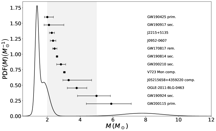
4 Conclusions
The size and density of the available compact object sample has greatly grown since their existence was first confirmed in the 1960s, with the sample of NSs surpassing 100 and that of Galactic BHs reaching 35 objects, while the GW observations from LVK have already detected more than 150 BHs and around 10 NSs at high redshift. Slowly, this growing sample has allowed us to start to see the shape of the underlying compact object mass distribution, provided biases do not dominate the samples. Once thought to be clustered around a canonical mass of , today NSs have been shown beyond doubt to have masses , with at least two peaks in the mass distribution. More recently, growing evidence suggests that their maximum mass might be closer to . This slow upward shift of the maximum NS mass value serves also as a cautionary tale with regard to the BH mass distribution, which is still based on only a few tens of measurements. As the canonical model for NS masses changed considerably while the sample was below objects, the BH sample may still need an accumulation of reliable data points before it can properly constrain the shape of the physical mass distribution. It is expected that BHs and a higher number of NSs should exist in the Galaxy, originating from a great diversity of evolutionary paths which we are only starting to understand. Progress in this front will also be needed before we can properly evaluate the degree of completeness of the sample due to observational biases.
Conceptualization, L.M.S., A.B., R.R.A.B., L.S.R., P.H.R.S.M. and J.E.H.; methodology, L.M.S., A.B., R.R.A.B., L.S.R., P.H.R.S.M. and J.E.H; formal analysis,, L.M.S., A.B., R.R.A.B., L.S.R., P.H.R.S.M. and J.E.H; investigation,, L.M.S., A.B., R.R.A.B., L.S.R., P.H.R.S.M. and J.E.H; data curation, , L.M.S., A.B., R.R.A.B., L.S.R., P.H.R.S.M. and J.E.H; writing-original draft preparation, , L.M.S., A.B., R.R.A.B., L.S.R., P.H.R.S.M. and J.E.H; writing-review and editing, , L.M.S., A.B., R.R.A.B., L.S.R., P.H.R.S.M. and J.E.H. All authors have read and agreed to the published version of the manuscript.
This research was funded by the Fapesp Agency through the grant 13/26258-4 and 2020/08518-2 and the CNPq (Federal Government) for the award of a Research Fellowship to J.E.H. L.M.S. acknowledges CNPq for financial support. The CAPES Agency (Federal Government) is acknowledged for financial support in the form of scholarships.
All observational data reported in this work is available within the quoted references. All data compiled and calculated in Tables 12 and 13 is publicly available in https://doi.org/10.5281/zenodo.7508626.
Acknowledgements.
We would like to thank the anonymous referees for their careful reports on the manuscript which helped lead to a more complete final version. This work has also made extensive use of NASA's Astrophysics Data System (ADS). \conflictsofinterestThe authors declare no conflict of interest. \reftitleReferencesReferences
- Walter et al. (1996) Walter, F.M.; Wolk, S.J.; Neuhäuser, R. Discovery of a nearby isolated neutron star. Nature 1996, 379, 233–235. https://doi.org/10.1038/379233a0.
- Zampieri et al. (2001) Zampieri, L.; Campana, S.; Turolla, R.; Chieregato, M.; Falomo, R.; Fugazza, D.; Moretti, A.; Treves, A. 1RXS J214303.7+065419/RBS 1774: A new Isolated Neutron Star candidate. Astron. Astrophys. 2001, 378, L5–L9. https://doi.org/10.1051/0004-6361:20011151.
- Turolla (2009) Turolla, R. Isolated Neutron Stars: The Challenge of Simplicity. In Proceedings of the Astrophysics and Space Science Library; Becker, W., Ed.; Springer: Berlin, Germany 2009; Volume 357, p. 141. https://doi.org/10.1007/978-3-540-76965-1_7.
- Ertan et al. (2014) Ertan, Ü.; Çalışkan, Ş.; Benli, O.; Alpar, M.A. Long-term evolution of dim isolated neutron stars. Mon. Not. R. Astron. Soc. 2014, 444, 1559–1565. https://doi.org/10.1093/mnras/stu1523.
- Esposito et al. (2021) Esposito, P.; Rea, N.; Israel, G.L. Magnetars: A Short Review and Some Sparse Considerations. In Proceedings of the Astrophysics and Space Science Library; Belloni, T.M.; Méndez, M.; Zhang, C., Eds.; Astrophysics and Space Science Library: New York, NY, USA, 2021, Volume 461, pp. 97–142, https://doi.org/10.1007/978-3-662-62110-3_3.
- De Luca (2017) De Luca, A. Central compact objects in supernova remnants. In Proceedings of the Journal of Physics Conference Series; IOP Publishing: Bristol, UK, 2017, Volume 932, p. 012006, https://doi.org/10.1088/1742-6596/932/1/012006.
- Mayer and Becker (2021) Mayer, M.G.F.; Becker, W. A kinematic study of central compact objects and their host supernova remnants. Astron. Astrophys. 2021, 651, A40. https://doi.org/10.1051/0004-6361/202141119.
- Ho (2013) Ho, W.C.G. Central compact objects and their magnetic fields. In Proceedings of the Neutron Stars and Pulsars: Challenges and Opportunities after 80 Years; van Leeuwen, J., Ed.; 2013; Volume 291, pp. 101–106. Publisher: Cambridge University Press (Cambridge) https://doi.org/10.1017/S1743921312023289.
- Ho et al. (2021) Ho, W.C.G.; Zhao, Y.; Heinke, C.O.; Kaplan, D.L.; Shternin, P.S.; Wijngaarden, M.J.P. X-ray bounds on cooling, composition, and magnetic field of the Cassiopeia A neutron star and young central compact objects. Mon. Not. R. Astron. Soc. 2021, 506, 5015–5029. https://doi.org/10.1093/mnras/stab2081.
- Abhishek et al. (2022) Abhishek, Malusare, N.; Tanushree, N.; Hegde, G.; Konar, S. Radio pulsar sub-populations (II): The mysterious RRATs. J. Astrophys. Astron. 2022, 43, 75. https://doi.org/10.1007/s12036-022-09862-3.
- Keane and McLaughlin (2011) Keane, E.F.; McLaughlin, M.A. Rotating radio transients. Bull. Astron. Soc. India 2011, 39, 333–352
- Hurley-Walker et al. (2022) Hurley-Walker, N.; Zhang, X.; Bahramian, A.; McSweeney, S.J.; O’Doherty, T.N.; Hancock, P.J.; Morgan, J.S.; Anderson, G.E.; Heald, G.H.; Galvin, T.J. A radio transient with unusually slow periodic emission. Nature 2022, 601, 526–530. https://doi.org/10.1038/s41586-021-04272-x.
- Corral-Santana et al. (2016) Corral-Santana, J.M.; Casares, J.; Muñoz-Darias, T.; Bauer, F.E.; Martínez-Pais, I.G.; Russell, D.M. BlackCAT: A catalogue of stellar-mass black holes in X-ray transients. Astron. Astrophys. 2016, 587, A61. https://doi.org/10.1051/0004-6361/201527130.
- Tetarenko et al. (2016) Tetarenko, B.E.; Sivakoff, G.R.; Heinke, C.O.; Gladstone, J.C. WATCHDOG: A Comprehensive All-sky Database of Galactic Black Hole X-ray Binaries. Astrophys. J., Suppl. Ser. 2016, 222, 15. https://doi.org/10.3847/0067-0049/222/2/15.
- Ingram and Motta (2019) Ingram, A.R.; Motta, S.E. A review of quasi-periodic oscillations from black hole X-ray binaries: Observation and theory. New Astron. Rev. 2019, 85, 101524. https://doi.org/10.1016/j.newar.2020.101524.
- Lam et al. (2022) Lam, C.Y.; Lu, J.R.; Udalski, A.; Bond, I.; Bennett, D.P.; Skowron, J.; Mróz, P.; Poleski, R.; Sumi, T.; Szymański, M.K.; et al. An Isolated Mass-gap Black Hole or Neutron Star Detected with Astrometric Microlensing. Astrophys. J. 2022, 933, L23. https://doi.org/10.3847/2041-8213/ac7442.
- Sahu et al. (2022) Sahu, K.C.; Anderson, J.; Casertano, S.; Bond, H.E.; Udalski, A.; Dominik, M.; Calamida, A.; Bellini, A.; Brown, T.M.; Rejkuba, M.; et al. An Isolated Stellar-mass Black Hole Detected through Astrometric Microlensing. Astrophys. J. 2022, 933,83. https://doi.org/10.3847/1538-4357/ac739e.
- Burrows and Vartanyan (2021) Burrows, A.; Vartanyan, D. Core-collapse supernova explosion theory. Nature 2021, 589, 29–39. https://doi.org/10.1038/s41586-020-03059-w.
- Ertl et al. (2020) Ertl, T.; Woosley, S.E.; Sukhbold, T.; Janka, H.T. The Explosion of Helium Stars Evolved with Mass Loss. Astrophys. J. 2020, 890, 51. https://doi.org/10.3847/1538-4357/ab6458.
- Tauris et al. (2013) Tauris, T.M.; Sanyal, D.; Yoon, S.C.; Langer, N. Evolution towards and beyond accretion-induced collapse of massive white dwarfs and formation of millisecond pulsars. Astron. Astrophys. 2013, 558, A39. https://doi.org/10.1051/0004-6361/201321662.
- Wang and Liu (2020) Wang, B.; Liu, D. The formation of neutron star systems through accretion-induced collapse in white-dwarf binaries. Res. Astron. Astrophys. 2020, 20, 135 https://doi.org/10.1088/1674-4527/20/9/135.
- Wang et al. (2022) Wang, B.; Liu, D.; Chen, H. Formation of millisecond pulsars with long orbital periods by accretion-induced collapse of white dwarfs. Mon. Not. R. Astron. Soc. 2022, 510, 6011–6021. https://doi.org/10.1093/mnras/stac114.
- Bailyn et al. (1998) Bailyn, C.D.; Jain, R.K.; Coppi, P.; Orosz, J.A. The Mass Distribution of Stellar Black Holes. Astrophys. J. 1998, 499, 367–374. https://doi.org/10.1086/305614.
- Özel et al. (2010) Özel, F.; Psaltis, D.; Narayan, R.; McClintock, J.E. THE BLACK HOLE MASS DISTRIBUTION IN THE GALAXY. Astrophys. J. 2010, 725, 1918. https://doi.org/10.1088/0004-637X/725/2/1918.
- Farr et al. (2011) Farr, W.M.; Sravan, N.; Cantrell, A.; Kreidberg, L.; Bailyn, C.D.; Mandel, I.; Kalogera, V. THE MASS DISTRIBUTION OF STELLAR-MASS BLACK HOLES. Astrophys. J. 2011, 741, 103. https://doi.org/10.1088/0004-637X/741/2/103.
- Fryer et al. (2012) Fryer, C.L.; Belczynski, K.; Wiktorowicz, G.; Dominik, M.; Kalogera, V.; Holz, D.E. Compact Remnant Mass Function: Dependence on the Explosion Mechanism and Metallicity. Astrophys. J. 2012, 749, 91. https://doi.org/10.1088/0004-637X/749/1/91.
- Belczynski et al. (2012) Belczynski, K.; Wiktorowicz, G.; Fryer, C.L.; Holz, D.E.; Kalogera, V. Missing Black Holes Unveil the Supernova Explosion Mechanism. Astrophys. J. 2012, 757, 91. https://doi.org/10.1088/0004-637X/757/1/91.
- Farah et al. (2022) Farah, A.; Fishbach, M.; Essick, R.; Holz, D.E.; Galaudage, S. Bridging the Gap: Categorizing Gravitational-wave Events at the Transition between Neutron Stars and Black Holes. Astrophys. J. 2022, 931, 108. https://doi.org/10.3847/1538-4357/ac5f03.
- de Sá et al. (2022) de Sá, L.M.; Bernardo, A.; Bachega, R.R.A.; Horvath, J.E.; Rocha, L.S.; Moraes, P.H.R.S. Quantifying the Evidence Against a Mass Gap between Black Holes and Neutron Stars. Astrophys. J. 2022, 941, 130. https://doi.org/10.3847/1538-4357/aca076.
- Ye and Fishbach (2022) Ye, C.; Fishbach, M. Inferring the Neutron Star Maximum Mass and Lower Mass Gap in Neutron Star–Black Hole Systems with Spin. Astrophys. J. 2022, 937, 73. https://doi.org/10.3847/1538-4357/ac7f99.
- Landau (1932) Landau, L. On the Theory of Stars. Phys. Z. Sowjetunion 1932, 1, 285–288.
- Baade and Zwicky (1934) Baade, W.; Zwicky, F. On Super-Novae. Proc. Natl. Acad. Sci. USA 1934, 20, 254–259. https://doi.org/10.1073/pnas.20.5.254.
- Hewish et al. (1968) Hewish, A.; Bell, S.J.; Pilkington, J.D.H.; Scott, P.F.; Collins, R.A. Observation of a Rapidly Pulsating Radio Source. Nature 1968, 217, 709–713. Number: 5130 Publisher: Nature Publishing Group, https://doi.org/10.1038/217709a0.
- Pacini (1968) Pacini, F. Rotating Neutron Stars, Pulsars and Supernova Remnants. Nature 1968, 219, 145–146. https://doi.org/10.1038/219145a0.
- Gold (1968) Gold, T. Rotating Neutron Stars as the Origin of the Pulsating Radio Sources. Nature 1968, 218, 731–732. https://doi.org/10.1038/218731a0.
- Bisnovatyi-Kogan (1992) Bisnovatyi-Kogan, G.S. The Neutron Star Population in the Galaxy. In Proceedings of IAU Symposium #149; Barbuy, B.; Renzini, A., Eds.; Spinger: Dordrecht, The Netherlands 1992; Volume 149, p. 379.
- Lyne et al. (1985) Lyne, A.G.; Manchester, R.N.; Taylor, J.H. The galactic population of pulsars. Mon. Not. R. Astron. Soc. 1985, 213, 613–639. https://doi.org/10.1093/mnras/213.3.613.
- Dirson et al. (2022) Dirson, L.; Pétri, J.; Mitra, D. The Galactic population of canonical pulsars. Astron. Astrophys. 2022, 667, A82. https://doi.org/10.1051/0004-6361/202243305.
- Kaspi (2010) Kaspi, V.M. Grand unification of neutron stars. Proc. Natl. Acad. Sci. USA 2010, 107, 7147–7152. https://doi.org/10.1073/pnas.1000812107.
- Rutledge et al. (2008) Rutledge, R.E.; Fox, D.B.; Shevchuk, A.H. Discovery of an Isolated Compact Object at High Galactic Latitude. Astrophys. J. 2008, 672, 1137–1143. https://doi.org/10.1086/522667.
- Potekhin et al. (2015) Potekhin, A.Y.; De Luca, A.; Pons, J.A. Neutron Stars—Thermal Emitters. Space Sci. Rev. 2015, 191, 171–206, https://doi.org/10.1007/s11214-014-0102-2.
- Agar et al. (2021) Agar, C.H.; Weltevrede, P.; Bondonneau, L.; Grießmeier, J.M.; Hessels, J.W.T.; Huang, W.J.; Karastergiou, A.; Keith, M.J.; Kondratiev, V.I.; Künsemöller, J.; et al. A broad-band radio study of PSR J0250+5854: the slowest spinning radio pulsar known. Mon. Not. R. Astron. Soc. 2021, 508, 1102–1114. https://doi.org/10.1093/mnras/stab2496.
- Morello et al. (2020) Morello, V.; Keane, E.F.; Enoto, T.; Guillot, S.; Ho, W.C.G.; Jameson, A.; Kramer, M.; Stappers, B.W.; Bailes, M.; Barr, E.D.; et al. The SUrvey for Pulsars and Extragalactic Radio Bursts – IV. Discovery and polarimetry of a 12.1-s radio pulsar. Mon. Not. R. Astron. Soc. 2020, 493, 1165–1177. https://doi.org/10.1093/mnras/staa321.
- Young et al. (1999) Young, M.D.; Manchester, R.N.; Johnston, S. A radio pulsar with an 8.5-second period that challenges emission models. Nature 1999, 400, 848–849. https://doi.org/10.1038/23650.
- Turolla and Esposito (2013) Turolla, R.; Esposito, P. Low-magnetic-field magnetars. Int. J. Mod. Phys. D 2013, 22, 1330024. https://doi.org/10.1142/S0218271813300243.
- Caleb et al. (2022) Caleb, M.; Heywood, I.; Rajwade, K.; Malenta, M.; Stappers, B.W.; Barr, E.; Chen, W.; Morello, V.; Sanidas, S.; van den Eijnden, J.; et al. Discovery of a radio-emitting neutron star with an ultra-long spin period of 76 s. Nat. Astron. 2022, 6, 828–836. https://doi.org/10.1038/s41550-022-01688-x.
- Buckley et al. (2017) Buckley, D.A.H.; Meintjes, P.J.; Potter, S.B.; Marsh, T.R.; Gänsicke, B.T. Polarimetric evidence of a white dwarf pulsar in the binary system AR Scorpii. Nat. Astron. 2017, 1, 29. https://doi.org/10.1038/s41550-016-0029.
- Viganò et al. (2013) Viganò, D.; Rea, N.; Pons, J.A.; Perna, R.; Aguilera, D.N.; Miralles, J.A. Unifying the observational diversity of isolated neutron stars via magneto-thermal evolution models. Mon. Not. R. Astron. Soc. 2013, 434, 123–141. https://doi.org/10.1093/mnras/stt1008.
- Igoshev et al. (2021) Igoshev, A.P.; Popov, S.B.; Hollerbach, R. Evolution of Neutron Star Magnetic Fields. Universe 2021, 7, 351. https://doi.org/10.3390/universe7090351.
- Benvenuto et al. (2014) Benvenuto, O.G.; De Vito, M.A.; Horvath, J.E. Understanding the Evolution of Close Binary Systems with Radio Pulsars. Astrophys. J. 2014, 786, L7. https://doi.org/10.1088/2041-8205/786/1/L7.
- Mendes et al. (2018) Mendes, C.; de Avellar, M.G.B.; Horvath, J.E.; Souza, R.A.d.; Benvenuto, O.G.; De Vito, M.A. Magnetic field decay in black widow pulsars. Mon. Not. R. Astron. Soc. 2018, 475, 2178–2184. https://doi.org/10.1093/mnras/stx3319.
- Igoshev and Popov (2020) Igoshev, A.P.; Popov, S.B. Braking indices of young radio pulsars: theoretical perspective. Mon. Not. R. Astron. Soc. 2020, 499, 2826–2835. https://doi.org/10.1093/mnras/staa3070.
- Allen and Horvath (1997) Allen, M.P.; Horvath, J.E. Glitches, torque evolution and the dynamics of young pulsars. Mon. Not. R. Astron. Soc. 1997, 287, 615–621. https://doi.org/10.1093/mnras/287.3.615.
- Yoneyama et al. (2019) Yoneyama, T.; Hayashida, K.; Nakajima, H.; Matsumoto, H. Unification of strongly magnetized neutron stars with regard to X-ray emission from hot spots. Astron. Nachrichten 2019, 340, 221–225. Available online: https://onlinelibrary.wiley.com/doi/pdf/10.1002/asna.201913593 (accessed on 21 Dec 2022)https://doi.org/10.1002/asna.201913593.
- Hurley (2010) Hurley, K. Soft gamma repeaters. Mem. Soc. Astron. Ital. 2010, 81, 432.
- Kaspi (2007) Kaspi, V.M. Recent progress on anomalous X-ray pulsars. Astrophys. Space Sci. 2007, 308, 1–11. https://doi.org/10.1007/s10509-007-9309-y.
- Keane (2016) Keane, E.F. Classifying RRATs and FRBs. Mon. Not. R. Astron. Soc. 2016, 459, 1360–1362. https://doi.org/10.1093/mnras/stw767.
- Kaspi and Kramer (2016) Kaspi, V.M.; Kramer, M. Radio Pulsars: The Neutron Star Population & Fundamental Physics. arXiv 2016, arXiv:1602.07738,
- Beniamini et al. (2022) Beniamini, P.; Wadiasingh, Z.; Hare, J.; Rajwade, K.; Younes, G.; van der Horst, A.J. Evidence for an abundant old population of Galactic Ultra long period magnetars and implications for fast radio bursts. arXiv 2022, arXiv:2210.09323. https://doi.org/10.48550/arxiv.2210.09323.
- Rocha et al. (2021) Rocha, L.S.; Bachega, R.R.A.; Horvath, J.E.; Moraes, P.H.R.S. The maximum mass of neutron stars may be higher than expected: an inference from binary systems. arXiv 2021, arXiv:2107.08822. https://doi.org/10.48550/ARXIV.2107.08822.
- Postnov and Prokhorov (2001) Postnov, K.A.; Prokhorov, M.E. The Relation between the Observed Mass Distribution for Compact Stars and the Mechanism for Supernova Explosions. Astron. Rep. 2001, 45, 899–907. https://doi.org/10.1134/1.1416279.
- Valentim et al. (2011) Valentim, R.; Rangel, E.; Horvath, J. On the mass distribution of neutron stars. Mon. Not. R. Astron. Soc. 2011, 414, 1427–1431.
- Özel and Freire (2016) Özel, F.; Freire, P. Masses, radii, and the equation of state of neutron stars. Annu. Rev. Astron. Astrophys. 2016, 54, 401–440.
- Kiziltan et al. (2013) Kiziltan, B.; Kottas, A.; De Yoreo, M.; Thorsett, S.E. The neutron star mass distribution. Astrophys. J. 2013, 778, 66.
- Zhang et al. (1997) Zhang, W.; Strohmayer, T.; Swank, J. Neutron star masses and radii as inferred from kilohertz quasi-periodic oscillations. Astrophys. J. 1997, 482, L167.
- Alsing et al. (2018) Alsing, J.; Silva, H.O.; Berti, E. Evidence for a maximum mass cut-off in the neutron star mass distribution and constraints on the equation of state. Mon. Not. R. Astron. Soc. 2018, 478, 1377–1391.
- Horvath et al. (2022) Horvath, J.; Rocha, L.; Bernardo, A.C.; de Avellar, M.; Valentim, R. Birth events, masses and the maximum mass of Compact Stars. In Astrophysics in the XXI Century with Compact Stars; Vasconcellos, C.Z., Weber, F., Eds.; World Scientific Publishing: Singapore, Singapore 2022; pp. 1–51.
- Rhoades and Ruffini (1974) Rhoades, C.E.; Ruffini, R. Maximum Mass of a Neutron Star. Phys. Rev. Lett. 1974, 32, 324–327. https://doi.org/10.1103/PhysRevLett.32.324.
- Margalit and Metzger (2017) Margalit, B.; Metzger, B.D. Constraining the Maximum Mass of Neutron Stars from Multi-messenger Observations of GW170817. Astrophys. J. Lett. 2017, 850, L19. https://doi.org/10.3847/2041-8213/aa991c.
- Rezzolla et al. (2018) Rezzolla, L.; Most, E.R.; Weih, L.R. Using Gravitational-wave Observations and Quasi-universal Relations to Constrain the Maximum Mass of Neutron Stars. Astrophys. J. Lett. 2018, 852, L25. https://doi.org/10.3847/2041-8213/aaa401.
- Ruiz et al. (2018) Ruiz, M.; Shapiro, S.L.; Tsokaros, A. GW170817, general relativistic magnetohydrodynamic simulations, and the neutron star maximum mass. Phys. Rev. D 2018, 97, 021501, https://doi.org/10.1103/PhysRevD.97.021501.
- Shibata et al. (2019) Shibata, M.; Zhou, E.; Kiuchi, K.; Fujibayashi, S. Constraint on the maximum mass of neutron stars using GW170817 event. Phys. Rev. D 2019, 100, 023015. https://doi.org/10.1103/PhysRevD.100.023015.
- Ai et al. (2020) Ai, S.; Gao, H.; Zhang, B. What Constraints on the Neutron Star Maximum Mass Can One Pose from GW170817 Observations? Astrophys. J. 2020, 893, 146. https://doi.org/10.3847/1538-4357/ab80bd.
- Romani et al. (2021) Romani, R.; Kandel, D.; Filippenko, A.; Brink, T.; Zheng, W. PSR J0952-0607: The Fastest and Heaviest Known Galactic Neutron Star . Astrophys. J. Lett. 2022, 934, L17 .
- Ecker and Rezzolla (2022) Ecker, C.; Rezzolla, L. Impact of large-mass constraints on the properties of neutron stars. arXiv 2022, arXiv:2209.08101,
- The LIGO Scientific Collaboration et al. (2021) Abbott, R.; Abbott, T.D.; Acernese, F.; Ackley, K.; Adams, C.; Adhikari, N.; Adhikari, R.X.; Adya, V.B.; Affeldt, C.; Agarwal, D.; et al. GWTC-3: Compact Binary Coalescences Observed by LIGO and Virgo During the Second Part of the Third Observing Run. arXiv 2021, arXiv:2111.03606. https://doi.org/10.48550/ARXIV.2111.03606.
- Doroshenko et al. (2022) Doroshenko, V.; Suleimanov, V.; Pühlhofer, G.; Santangelo, A. A strangely light neutron star within a supernova remnant. Nat. Astron. 2022, 6, 1444–1451. https://doi.org/10.1038/s41550-022-01800-1.
- Di Clemente et al. (2022) Di Clemente, F.; Drago, A.; Pagliara, G. Is the compact object associated with HESS J1731-347 a strange quark star? arXiv 2022, arXiv:2211.07485.
- Weber (2005) Weber, F. Strange quark matter and compact stars. Prog. Part. Nucl. Phys. 2005, 54, 193–288.
- Martinez et al. (2015) Martinez, J.G.; Stovall, K.; Freire, P.C.C.; Deneva, J.S.; Jenet, F.A.; McLaughlin, M.A.; Bagchi, M.; Bates, S.D.; Ridolfi, A. PULSAR J0453+1559: A DOUBLE NEUTRON STAR SYSTEM WITH A LARGE MASS ASYMMETRY. Astrophys. J. 2015, 812, 143. https://doi.org/10.1088/0004-637x/812/2/143.
- Fonseca et al. (2016) Fonseca, E.; Pennucci, T.T.; Ellis, J.A.; Stairs, I.H.; Nice, D.J.; Ransom, S.M.; Demorest, P.B.; Arzoumanian, Z.; Crowter, K.; Dolch, T.; et al. The NANOGrav Nine-year Data Set: Mass and Geometric Measurements of Binary Millisecond Pulsars. Astrophys. J. 2016, 832, 167. https://doi.org/10.3847/0004-637X/832/2/167.
- Lattimer (2019) Lattimer, J.M. Neutron Star Mass and Radius Measurements. Universe 2019, 5, 159. https://doi.org/10.3390/universe5070159.
- Riley and et al. (2021) Riley, T.; et al.. A NICER View of the Massive Pulsar PSR J0740+6620 Informed by Radio Timing and XMM-Newton Spectroscopy. Astrophys. J. 2021, 918, L27.
- Riley and et al. (2019) Riley, T.; et al.. A NICER View of PSR J0030+0451: Millisecond Pulsar Parameter Estimation. Astrophys. J. 2019, 887, L21.
- Horvath and Moraes (2021) Horvath, J.; Moraes, P. H. R. S. Modeling a 2.5Mo compact star with quark matter . Int. Jour. Mod. Phys. D 2021, 30, 2150016.
- Einstein (1915) Einstein, A. Die Feldgleichungen der Gravitation; Sitzungsberichte der Preussischen Akademie der Wissenschaften zu Berlin: Berlin, Germany, 1915; pp. 844–847.
- Schwarzschild (1916) Schwarzschild, K. On the Gravitational Field of a Mass Point According to Einstein’s Theory. Abh. Konigl. Preuss. Akad. 1916, 189–196.
- Kerr (1963) Kerr, R.P. Gravitational Field of a Spinning Mass as an Example of Algebraically Special Metrics. Phys. Rev. Lett. 1963, 11, 237–238. https://doi.org/10.1103/PhysRevLett.11.237.
- Newman et al. (1965) Newman, E.T.; Couch, E.; Chinnapared, K.; Exton, A.; Prakash, A.; Torrence, R. Metric of a Rotating, Charged Mass. J. Math. Phys. 1965, 6, 918–919. https://doi.org/10.1063/1.1704351.
- ’t Hooft (1991) ’t Hooft, G. The Black hole horizon as a quantum surface. Phys. Scr. 1991, 36, 247–252. https://doi.org/10.1088/0031-8949/1991/T36/026.
- Hawking (2015) Hawking, S.W. The information paradox for black holes. arXiv 2015, arXiv:1509.01147.
- Susskind (2006) Susskind, L. The paradox of quantum black holes. Nature Physics 2006, 2, 665–677.
- Oppenheimer and Volkoff (1939) Oppenheimer, J.R.; Volkoff, G.M. On Massive Neutron Cores. Phys. Rev. 1939, 55, 374–381. https://doi.org/10.1103/PhysRev.55.374.
- Tolman (1939) Tolman, R.C. Static Solutions of Einstein’s Field Equations for Spheres of Fluid. Phys. Rev. 1939, 55, 364–373. https://doi.org/10.1103/PhysRev.55.364.
- Zel’dovich (1964) Zel’dovich, Y.B. The fate of a star, and the liberation of gravitation energy in accretion. Dokl. Akad. Nauk SSSR 1964, 155, 67–69.
- Salpeter (1964) Salpeter, E.E. Accretion of Interstellar Matter by Massive Objects. Astrophys. J. 1964, 140, 796–800. https://doi.org/10.1086/147973.
- Bolton (1972) Bolton, C.T. Identification of Cygnus X-1 with HDE 226868. Nature 1972, 235, 271–273. https://doi.org/10.1038/235271b0.
- Webster and Murdin (1972) Webster, B.L.; Murdin, P. Cygnus X-1-a Spectroscopic Binary with a Heavy Companion ? Nature 1972, 235, 37–38. https://doi.org/10.1038/235037a0.
- Gelino and Harrison (2003) Gelino, D.M.; Harrison, T.E. GRO J0422+32: The Lowest Mass Black Hole? Astrophys. J. 2003, 599, 1254–1259. https://doi.org/10.1086/379311.
- Liu et al. (2019) Liu, J.; Zhang, H.; Howard, A.W.; Bai, Z.; Lu, Y.; Soria, R.; Justham, S.; Li, X.; Zheng, Z.; Wang, T.; et al. A wide star–black-hole binary system from radial-velocity measurements. Nature 2019, 575, 618–621. https://doi.org/10.1038/s41586-019-1766-2.
- Thompson et al. (2019) Thompson, T.A.; Kochanek, C.S.; Stanek, K.Z.; Badenes, C.; Post, R.S.; Jayasinghe, T.; Latham, D.W.; Bieryla, A.; Esquerdo, G.A.; Berlind, P.; et al. A noninteracting low-mass black hole-giant star binary system. Science 2019, 366, 637–640. https://doi.org/10.1126/science.aau4005.
- El-Badry et al. (2022) El-Badry, K.; Rix, H.W.; Quataert, E.; Howard, A.W.; Isaacson, H.; Fuller, J.; Hawkins, K.; Breivik, K.; Wong, K.W.K.; Rodriguez, A.C.; et al. A Sun-like star orbiting a black hole. Mon. Not. R. Astron. Soc. 2022, 518, 1057–1085. https://doi.org/10.1093/mnras/stac3140.
- King (2006) King, A.R. Accretion in compact binaries. In Compact Stellar X-ray Sources; Cambridge University Press: Cambridge, UK, 2006; Volume 39, pp. 507–546.
- Shakura and Sunyaev (1973) Shakura, N.I.; Sunyaev, R.A. Black holes in binary systems. Observational appearance. Astron. Atrophys. 1973, 24, 337–355.
- Shapiro et al. (1976) Shapiro, S.L.; Lightman, A.P.; Eardley, D.M. A two-temperature accretion disk model for Cygnus X-1: structure and spectrum. Astrophys. J. 1976, 204, 187–199. https://doi.org/10.1086/154162.
- Frank et al. (2002) Frank, J.; King, A.; Raine, D.J. Accretion Power in Astrophysics, 3rd ed.; Cambridge University Press: Cambridge, UK, 2002.
- Liao et al. (2020) Liao, Z.; Liu, J.; Zheng, X.; Gou, L. Spectral evidence of an accretion disc in wind-fed X-ray pulsar Vela X-1 during an unusual spin-up period. Mon. Not. R. Astron. Soc. 2020, 492, 5922–5929. https://doi.org/10.1093/mnras/staa162.
- Tauris and van den Heuvel (2006) Tauris, T.M.; van den Heuvel, E.P.J. Formation and evolution of compact stellar X-ray sources. In Compact Stellar X-ray Sources; Cambridge University Press: Cambridge, UK, 2006; Volume 39, pp. 623–665.
- Hameury (2020) Hameury, J. A review of the disc instability model for dwarf novae, soft X-ray transients and related objects. Adv. Space Res. 2020, 66, 1004–1024. https://doi.org/https://doi.org/10.1016/j.asr.2019.10.022.
- Tremaine and Davis (2014) Tremaine, S.; Davis, S.W. Dynamics of warped accretion discs. Mon. Not. R. Astron. Soc. 2014, 441, 1408–1434. Available online: https://academic.oup.com/mnras/article-pdf/441/2/1408/3724550/stu663.pdf (accessed on 21 Dec 2022). https://doi.org/10.1093/mnras/stu663.
- Abarr and Krawczynski (2020) Abarr, Q.; Krawczynski, H. Exploring the Physics of Warped Accretion Disks with the Imaging X-ray Polarimetry Explorer. In Proceedings of the American Astronomical Society Meeting Abstracts #235. Am. Astron. Soc. Meet. Abstr. 2020, 235, 346.02.
- Bagnoli et al. (2015) Bagnoli, T.; in’t Zand, J.J.M.; D’Angelo, C.R.; Galloway, D.K. A population study of type II bursts in the Rapid Burster. Mon. Not. R. Astron. Soc. 2015, 449, 268–287. https://doi.org/10.1093/mnras/stv330.
- Reig (2011) Reig, P. Be/X-ray binaries. Astrophys. Space Sci. 2011, 332, 1–29. https://doi.org/10.1007/s10509-010-0575-8.
- Ribó et al. (2017) Ribó, M.; Munar-Adrover, P.; Paredes, J.M.; Marcote, B.; Iwasawa, K.; Moldón, J.; Casares, J.; Migliari, S.; Paredes-Fortuny, X. The First Simultaneous X-Ray/Radio Detection of the First Be/BH System MWC 656. Astrophys. J. Lett. 2017, 835, L33. https://doi.org/10.3847/2041-8213/835/2/L33.
- Lutovinov et al. (2013) Lutovinov, A.A.; Revnivtsev, M.G.; Tsygankov, S.S.; Krivonos, R.A. Population of persistent high-mass X-ray binaries in the Milky Way. Mon. Not. R. Astron. Soc. 2013, 431, 327–341. https://doi.org/10.1093/mnras/stt168.
- Sguera et al. (2005) Sguera, V.; Barlow, E.J.; Bird, A.J.; Clark, D.J.; Dean, A.J.; Hill, A.B.; Moran, L.; Shaw, S.E.; Willis, D.R.; Bazzano, A.; et al. INTEGRAL observations of recurrent fast X-ray transient sources. Astron. Astrophys. 2005, 444, 221–231. https://doi.org/10.1051/0004-6361:20053103.
- Negueruela et al. (2006) Negueruela, I.; Smith, D.M.; Reig, P.; Chaty, S.; Torrejón, J.M. Supergiant Fast X-ray Transients: A New Class of High Mass X-ray Binaries Unveiled by INTEGRAL. In Proceedings of the The X-ray Universe 2005; Wilson, A., Ed.; ESA Publications Division: Noordwijk, The Netherlands 2006; Volume 604,p. 165.
- Sidoli (2017) Sidoli, L. Supergiant Fast X-ray Transients-A short review. arXiv 2017, arXiv:1710.03943. https://doi.org/10.48550/ARXIV.1710.03943.
- Corbel (2011) Corbel, S. Microquasars: an observational review. In Proceedings of IAU Symposium #275; Romero, G.E., Sunyaev, R.A., Belloni, T., Eds.; Cambridge University Press: Cambridge, UK 2011; pp. 205–214. https://doi.org/10.1017/S1743921310016054.
- McClintock and Remillard (2006) McClintock, J.E.; Remillard, R.A., Black hole binaries. In Compact Stellar X-ray Sources; Lewin, W., van der Klis, M., Eds.; Cambridge Astrophysics, Cambridge University Press: Cambridge, UK, 2006; p. 157–214. https://doi.org/10.1017/CBO9780511536281.005.
- Titarchuk and Fiorito (2004) Titarchuk, L.; Fiorito, R. Spectral Index and Quasi-Periodic Oscillation Frequency Correlation in Black Hole Sources: Observational Evidence of Two Phases and Phase Transition in Black Holes. Astrophys. J. 2004, 612, 988–999. https://doi.org/10.1086/422573.
- Charles and Coe (2006) Charles, P.A.; Coe, M.J. Optical, ultraviolet and infrared observations of X-ray binaries. In Compact Stellar X-ray Sources; Cambridge University Press: Cambridge, UK, 2006; Volume 39, pp. 215–265.
- Kreidberg et al. (2012) Kreidberg, L.; Bailyn, C.D.; Farr, W.M.; Kalogera, V. Mass Measurements of Black Holes in X-Ray Transients: Is There a Mass Gap? Astrophys. J. 2012, 757, 36. https://doi.org/10.1088/0004-637X/757/1/36.
- Orosz et al. (2009) Orosz, J.A.; Steeghs, D.; McClintock, J.E.; Torres, M.A.P.; Bochkov, I.; Gou, L.; Narayan, R.; Blaschak, M.; Levine, A.M.; Remillard, R.A.; et al. A NEW DYNAMICAL MODEL FOR THE BLACK HOLE BINARY LMC X-1. Astrophys. J. 2009, 697, 573. https://doi.org/10.1088/0004-637X/697/1/573.
- Orosz et al. (2011) Orosz, J.A.; McClintock, J.E.; Aufdenberg, J.P.; Remillard, R.A.; Reid, M.J.; Narayan, R.; Gou, L. THE MASS OF THE BLACK HOLE IN CYGNUS X-1. Astrophys. J. 2011, 742, 84. https://doi.org/10.1088/0004-637X/742/2/84.
- Orosz et al. (2007) Orosz, J.A.; McClintock, J.E.; Narayan, R.; Bailyn, C.D.; Hartman, J.D.; Macri, L.; Liu, J.; Pietsch, W.; Remillard, R.A.; Shporer, A.; et al. A 15.65-solar-mass black hole in an eclipsing binary in the nearby spiral galaxy M 33. Nature 2007, 449, 872–875. https://doi.org/10.1038/nature06218.
- Cherepashchuk (2022) Cherepashchuk, A. Progress in Understanding the Nature of SS433. Universe 2022, 8, 13. https://doi.org/10.3390/universe8010013.
- Orosz (2003) Orosz, J.A. Inventory of black hole binaries. In Proceedings of IAU Symposium #212; Cambridge University Press: Cambridge, UK, 2003. Volume 212, 365.
- Greiner et al. (2001) Greiner, J.; Cuby, J.G.; McCaughrean, M.J. An unusually massive stellar black hole in the Galaxy. Nature 2001, 414, 522–525. https://doi.org/10.1038/35107019.
- Casares et al. (2009) Casares, J.; Orosz, J.A.; Zurita, C.; Shahbaz, T.; Corral-Santana, J.M.; McClintock, J.E.; Garcia, M.R.; Martínez-Pais, I.G.; Charles, P.A.; Fender, R.P.; et al. Refined Orbital Solution and Quiescent Variability in the Black Hole Transient GS 1354-64 (= BW Cir). Astrophys. J. Suppl. Ser. 2009, 181, 238–243. https://doi.org/10.1088/0067-0049/181/1/238.
- Casares et al. (2004) Casares, J.; Zurita, C.; Shahbaz, T.; Charles, P.A.; Fender, R.P. Evidence of a Black Hole in the X-Ray Transient GS 1354-64 (=BW Circini). Astrophys. J. 2004, 613, L133–L136. https://doi.org/10.1086/425145.
- Wu et al. (2015) Wu, J.; Orosz, J.A.; McClintock, J.E.; Steeghs, D.; Longa-Peña, P.; Callanan, P.J.; Gou, L.; Ho, L.C.; Jonker, P.G.; Reynolds, M.T.; et al. A Dynamical Study of the Black Hole X-Ray Binary Nova Muscae 1991. Astrophys. J. 2015, 806, 92. https://doi.org/10.1088/0004-637X/806/1/92.
- Wu et al. (2016) Wu, J.; Orosz, J.A.; McClintock, J.E.; Hasan, I.; Bailyn, C.D.; Gou, L.; Chen, Z. The Mass of the Black Hole in the X-ray Binary Nova Muscae 1991. Astrophys. J. 2016, 825, 46. https://doi.org/10.3847/0004-637X/825/1/46.
- González Hernández et al. (2014) González Hernández, J.I.; Rebolo, R.; Casares, J. Fast orbital decays of black hole X-ray binaries: XTE J1118+480 and A0620-00. Mon. Not. R. Astron. Soc. 2014, 438, L21–L25. https://doi.org/10.1093/mnrasl/slt150.
- Torres et al. (2004) Torres, M.A.P.; Callanan, P.J.; Garcia, M.R.; Zhao, P.; Laycock, S.; Kong, A.K.H. MMT Observations of the Black Hole Candidate XTE J1118+480 near and in Quiescence. Astrophys. J. 2004, 612, 1026–1033. https://doi.org/10.1086/422740.
- González Hernández et al. (2012) González Hernández, J.I.; Rebolo, R.; Casares, J. The Fast Spiral-in of the Companion Star to the Black Hole XTE J1118+480. Astrophys. J. 2012, 744, L25. https://doi.org/10.1088/2041-8205/744/2/L25.
- Hernández et al. (2008) Hernández, J.I.G.; Rebolo, R.; Israelian, G.; Filippenko, A.V.; Chornock, R.; Tominaga, N.; Umeda, H.; Nomoto, K. Chemical Abundances of the Secondary Star in the Black Hole X-Ray Binary XTE J1118+480. Astrophys. J. 2008, 679, 732. https://doi.org/10.1086/586888.
- Calvelo et al. (2009) Calvelo, D.E.; Vrtilek, S.D.; Steeghs, D.; Torres, M.A.P.; Neilsen, J.; Filippenko, A.V.; González Hernández, J.I. Doppler and modulation tomography of XTEJ1118+480 in quiescence. Mon. Not. R. Astron. Soc. 2009, 399, 539–549. https://doi.org/10.1111/j.1365-2966.2009.15304.x.
- Khargharia et al. (2012) Khargharia, J.; Froning, C.S.; Robinson, E.L.; Gelino, D.M. THE MASS OF THE BLACK HOLE IN XTE J1118+480. AJ 2012, 145, 21. https://doi.org/10.1088/0004-6256/145/1/21.
- Hernández and Casares (2010) Hernández, J.I.G.; Casares, J. Doppler tomography of the black hole binary A0620-00 and the origin of chromospheric emission in quiescent X-ray binaries. Astron. Astrophys. 2010, 516, A58. https://doi.org/10.1051/0004-6361/201014088.
- McClintock and Remillard (1986) McClintock, J.E.; Remillard, R.A. The Black Hole Binary A0620-00. Astrophys. J. 1986, 308, 110. https://doi.org/10.1086/164482.
- Neilsen et al. (2008) Neilsen, J.; Steeghs, D.; Vrtilek, S.D. The eccentric accretion disc of the black hole A0620-00. Mon. Not. R. Astron. Soc. 2008, 384, 849–862. https://doi.org/10.1111/j.1365-2966.2007.12599.x.
- Cantrell et al. (2010) Cantrell, A.G.; Bailyn, C.D.; Orosz, J.A.; McClintock, J.E.; Remillard, R.A.; Froning, C.S.; Neilsen, J.; Gelino, D.M.; Gou, L. The Inclination of the Soft X-Ray Transient A0620-00 and the Mass of its Black Hole. Astrophys. J. 2010, 710, 1127–1141. https://doi.org/10.1088/0004-637X/710/2/1127.
- Ioannou et al. (2004) Ioannou, Z.; Robinson, E.L.; Welsh, W.F.; Haswell, C.A. The Mass of the Black Hole in GS 2000+25. Astron. J. 2004, 127, 481–488. https://doi.org/10.1086/380215.
- Harlaftis et al. (1996) Harlaftis, E.T.; Horne, K.; Filippenko, A.V. The Mass Ratio and the Disk Image of the X-Ray Nova GS 2000+25. Publ. Astron. Soc. Pac. 1996, 108, 762. https://doi.org/10.1086/133799.
- Torres et al. (2021) Torres, M.A.P.; Jonker, P.G.; Casares, J.; Miller-Jones, J.C.A.; Steeghs, D. Delimiting the black hole mass in the X-ray transient MAXI J1659-152 with H spectroscopy. Mon. Not. R. Astron. Soc. 2021, 501, 2174–2181. https://doi.org/10.1093/mnras/staa3786.
- Mata Sánchez et al. (2021) Mata Sánchez, D.; Rau, A.; Álvarez Hernández, A.; van Grunsven, T.F.J.; Torres, M.A.P.; Jonker, P.G. Dynamical confirmation of a stellar mass black hole in the transient X-ray dipping binary MAXI J1305-704. Mon. Not. R. Astron. Soc. 2021, 506, 581–594. https://doi.org/10.1093/mnras/stab1714.
- Casares and Charles (1994) Casares, J.; Charles, P.A. Optical studies of V404 Cyg, the X-ray transient GS 2023+338. IV. The rotation speed of the companion star. Mon. Not. R. Astron. Soc. 1994, 271, L5–L9. https://doi.org/10.1093/mnras/271.1.L5.
- Khargharia et al. (2010) Khargharia, J.; Froning, C.S.; Robinson, E.L. Near-infrared Spectroscopy of Low-mass X-ray Binaries: Accretion Disk Contamination and Compact Object Mass Determination in V404 Cyg and Cen X-4. Astrophys. J. 2010, 716, 1105–1117. https://doi.org/10.1088/0004-637X/716/2/1105.
- Orosz et al. (2004) Orosz, J.A.; McClintock, J.E.; Remillard, R.A.; Corbel, S. Orbital Parameters for the Black Hole Binary XTE J1650-500. Astrophys. J. 2004, 616, 376–382. https://doi.org/10.1086/424892.
- Webb et al. (2000) Webb, N.A.; Naylor, T.; Ioannou, Z.; Charles, P.A.; Shahbaz, T. A TiO study of the black hole binary GRO J0422+32 in a very low state. Mon. Not. R. Astron. Soc. 2000, 317, 528–534. https://doi.org/10.1046/j.1365-8711.2000.03608.x.
- Remillard et al. (1996) Remillard, R.A.; Orosz, J.A.; McClintock, J.E.; Bailyn, C.D. Dynamical Evidence for a Black Hole in X-Ray Nova Ophiuchi 1977. Astrophys. J. 1996, 459, 226. https://doi.org/10.1086/176885.
- Harlaftis et al. (1997) Harlaftis, E.T.; Steeghs, D.; Horne, K.; Filippenko, A.V. A doppler map and mass-ration constraint for the black-hole X-ray Nova Ophiuchi 1977. Astron. J. 1997, 114, 1170–1175. https://doi.org/10.1086/118548.
- Hernández et al. (2008) Hernández, J.I.G.; Rebolo, R.; Israelian, G. The black hole binary nova Scorpii 1994 (GRO J1655-40): an improved chemical analysis. Astron. Astrophys. 2008, 478, 203–217. https://doi.org/10.1051/0004-6361:20077141.
- Beer and Podsiadlowski (2002) Beer, M.E.; Podsiadlowski, P. The quiescent light curve and the evolutionary state of GRO J1655-40. Mon. Not. R. Astron. Soc. 2002, 331, 351–360. https://doi.org/10.1046/j.1365-8711.2002.05189.x.
- Shahbaz (2003) Shahbaz, T. Determining the spectroscopic mass ratio in interacting binaries: application to X-Ray Nova Sco 1994. Mon. Not. R. Astron. Soc. 2003, 339, 1031–1040. https://doi.org/10.1046/j.1365- 8711.2003.06258.x.
- Greene et al. (2001) Greene, J.; Bailyn, C.D.; Orosz, J.A. Optical and Infrared Photometry of the Microquasar GRO J1655–40 in Quiescence. Astrophys. J. 2001, 554, 1290. https://doi.org/10.1086/321411.
- Corral-Santana et al. (2011) Corral-Santana, J.M.; Casares, J.; Shahbaz, T.; Zurita, C.; Martínez-Pais, I.G.; Rodríguez-Gil, P. Evidence for a black hole in the X-ray transient XTE J1859+226. Mon. Not. R. Astron. Soc. 2011, 413, L15–L19. https://doi.org/10.1111/j.1745-3933.2011.01022.x.
- Filippenko and Chornock (2001) Filippenko, A.V.; Chornock, R. XTE J1859+226. Int. Astron. Union Circ. 2001, 7644, 2.
- Sánchez et al. (2022) Sánchez, D.M.; Muñoz-Darias, T.; Cúneo, V.A.; Padilla, M.A.; Sánchez-Sierras, J.; Panizo-Espinar, G.; Casares, J.; Corral-Santana, J.M.; Torres, M.A.P. Hard-state Optical Wind during the Discovery Outburst of the Black Hole X-Ray Dipper MAXI J1803–298. Astrophys. J. Lett. 2022, 926, L10. https://doi.org/10.3847/2041-8213/ac502f.
- Torres et al. (2019) Torres, M.A.P.; Casares, J.; Jiménez-Ibarra, F.; Muñoz-Darias, T.; Armas Padilla, M.; Jonker, P.G.; Heida, M. Dynamical Confirmation of a Black Hole in MAXI J1820+070. Astrophys. J. 2019, 882, L21. https://doi.org/10.3847/2041-8213/ab39df.
- Torres et al. (2020) Torres, M.A.P.; Casares, J.; Jiménez-Ibarra, F.; Álvarez Hernández, A.; Muñoz-Darias, T.; Armas Padilla, M.; Jonker, P.G.; Heida, M. The Binary Mass Ratio in the Black Hole Transient MAXI J1820+070. Astrophys. J. 2020, 893, L37. https://doi.org/10.3847/2041-8213/ab863a.
- Atri et al. (2020) Atri, P.; Miller-Jones, J.C.A.; Bahramian, A.; Plotkin, R.M.; Deller, A.T.; Jonker, P.G.; Maccarone, T.J.; Sivakoff, G.R.; Soria, R.; Altamirano, D.; et al. A radio parallax to the black hole X-ray binary MAXI J1820+070. Mon. Not. R. Astron. Soc. 2020, 493, L81–L86. https://doi.org/10.1093/mnrasl/slaa010.
- Orosz et al. (2011) Orosz, J.A.; Steiner, J.F.; McClintock, J.E.; Torres, M.A.P.; Remillard, R.A.; Bailyn, C.D.; Miller, J.M. An Improved Dynamical Model for the Microquasar XTE J1550-564. Astrophys. J. 2011, 730, 75. https://doi.org/10.1088/0004-637X/730/2/75.
- Connors et al. (2020) Connors, R.M.T.; García, J.A.; Dauser, T.; Grinberg, V.; Steiner, J.F.; Sridhar, N.; Wilms, J.; Tomsick, J.; Harrison, F.; Licklederer, S. Evidence for Returning Disk Radiation in the Black Hole X-Ray Binary XTE J1550–564. Astrophys. J. 2020, 892, 47. https://doi.org/10.3847/1538-4357/ab7afc.
- Heida et al. (2017) Heida, M.; Jonker, P.G.; Torres, M.A.P.; Chiavassa, A. The Mass Function of GX 339–4 from Spectroscopic Observations of Its Donor Star. Astrophys. J. 2017, 846, 132. https://doi.org/10.3847/1538-4357/aa85df.
- Hynes et al. (2003) Hynes, R.I.; Steeghs, D.; Casares, J.; Charles, P.A.; O’Brien, K. Dynamical Evidence for a Black Hole in GX 339-4. Astrophys. J. 2003, 583, L95–L98. https://doi.org/10.1086/368108.
- Filippenko et al. (1999) Filippenko, A.V.; Leonard, D.C.; Matheson, T.; Li, W.; Moran, E.C.; Riess, A.G. A Black Hole in the X-Ray Nova Velorum 1993. Publ. Astron. Soc. Pac. 1999, 111, 969–979. https://doi.org/10.1086/316413.
- Macias et al. (2011) Macias, P.; Orosz, J.A.; Bailyn, C.D.; Buxton, M.M.; Schechter, P.L.; Remillard, R.A.; McClintock, J.E.; Steiner, J.F. A Refined Black Hole Mass for the X-ray Transient GRS 1009-45. Am. Astron. Soc. Meet. Abstr. 2011. 217, 143.04.
- Orosz et al. (2014) Orosz, J.A.; Steiner, J.F.; McClintock, J.E.; Buxton, M.M.; Bailyn, C.D.; Steeghs, D.; Guberman, A.; Torres, M.A.P. THE MASS OF THE BLACK HOLE IN LMC X-3. Astrophys. J. 2014, 794, 154. https://doi.org/10.1088/0004-637X/794/2/154.
- Orosz et al. (2001) Orosz, J.A.; Kuulkers, E.; van der Klis, M.; McClintock, J.E.; Garcia, M.R.; Callanan, P.J.; Bailyn, C.D.; Jain, R.K.; Remillard, R.A. A Black Hole in the Superluminal Source SAX J1819.3-2525 (V4641 Sgr). Astrophys. J. 2001, 555, 489–503. https://doi.org/10.1086/321442.
- MacDonald et al. (2014) MacDonald, R.K.D.; Bailyn, C.D.; Buxton, M.; Cantrell, A.G.; Chatterjee, R.; Kennedy-Shaffer, R.; Orosz, J.A.; Markwardt, C.B.; Swank, J.H. The Black Hole Binary V4641 Sagitarii: Activity in Quiescence and Improved Mass Determinations. Astrophys. J. 2014, 784, 2. https://doi.org/10.1088/0004-637X/784/1/2.
- Lindstrøm et al. (2005) Lindstrøm, C.; Griffin, J.; Kiss, L.L.; Uemura, M.; Derekas, A.; Mészáros, S.; Székely, P. New clues on outburst mechanisms and improved spectroscopic elements of the black hole binary V4641 Sagittarii. Mon. Not. R. Astron. Soc. 2005, 363, 882–890. https://doi.org/10.1111/j.1365-2966.2005.09483.x.
- Zhang et al. (2022) Zhang, Z.; Liu, H.; Abdikamalov, A.B.; Ayzenberg, D.; Bambi, C.; Zhou, M. Testing the Kerr Black Hole Hypothesis with GRS 1716-249 by Combining the Continuum Fitting and the Iron-line Methods. Astrophys. J. 2022, 924, 72. https://doi.org/10.3847/1538-4357/ac350e.
- Jana et al. (2021) Jana, A.; Jaisawal, G.K.; Naik, S.; Kumari, N.; Chatterjee, D.; Chatterjee, K.; Bhowmick, R.; Chakrabarti, S.K.; Chang, H.K.; Debnath, D. Accretion properties of MAXI J1813-095 during its failed outburst in 2018. Res. Astron. Astrophys. 2021, 21, 125. https://doi.org/10.1088/1674-4527/21/5/125.
- Shang et al. (2019) Shang, J.R.; Debnath, D.; Chatterjee, D.; Jana, A.; Chakrabarti, S.K.; Chang, H.K.; Yap, Y.X.; Chiu, C.L. Evolution of X-Ray Properties of MAXI J1535-571: Analysis with the TCAF Solution. Astrophys. J. 2019, 875, 4. https://doi.org/10.3847/1538-4357/ab0c1e.
- Molla et al. (2017) Molla, A.A.; Chakrabarti, S.K.; Debnath, D.; Mondal, S. Estimation of Mass of Compact Object in H 1743-322 From 2010 and 2011 Outbursts Using Tcaf Solution and Spectral Index–qpo Frequency Correlation. Astrophys. J. 2017, 834, 88. Publisher: The American Astronomical Society, https://doi.org/10.3847/1538-4357/834/1/88.
- Tursunov and Kološ (2018) Tursunov, A.A.; Kološ, M. Constraints on Mass, Spin and Magnetic Field of Microquasar H 1743-322 from Observations of QPOs. Phys. Atom. Nuclei 2018, 81, 279–282. https://doi.org/10.1134/S1063778818020187.
- Brocksopp et al. (1999) Brocksopp, C.; Tarasov, A.E.; Lyuty, V.M.; Roche, P. An improved orbital ephemeris for Cygnus X-1. Astron. Astrophys. 1999, 343, 861–864,
- Gies et al. (2003) Gies, D.R.; Bolton, C.T.; Thomson, J.R.; Huang, W.; McSwain, M.V.; Riddle, R.L.; Wang, Z.; Wiita, P.J.; Wingert, D.W.; Csák, B.; et al. Wind Accretion and State Transitions in Cygnus X-1. Astrophys. J. 2003, 583, 424. https://doi.org/10.1086/345345.
- Hutchings et al. (1987) Hutchings, J.B.; Crampton, D.; Cowley, A.P.; Bianchi, L.; Thompson, I.B. Optical and UV Spectroscopy of the Black Hole Binary Candidate LMC X-1. Astron. J. 1987, 94, 340. https://doi.org/10.1086/114475.
- Pietsch et al. (2006) Pietsch, W.; Haberl, F.; Sasaki, M.; Gaetz, T.J.; Plucinsky, P.P.; Ghavamian, P.; Long, K.S.; Pannuti, T.G. M33 X-7: ChASeM33 Reveals the First Eclipsing Black Hole X-Ray Binary. Astrophys. J. 2006, 646, 420. https://doi.org/10.1086/504704.
- Crowther et al. (2010) Crowther, P.A.; Barnard, R.; Carpano, S.; Clark, J.S.; Dhillon, V.S.; Pollock, A.M.T. NGC 300 X-1 is a Wolf-Rayet/black hole binary. Mon. Not. R. Astron. Soc. Lett. 2010, 403, L41–L45. https://doi.org/10.1111/j.1745-3933.2010.00811.x.
- Binder et al. (2021) Binder, B.A.; Sy, J.M.; Eracleous, M.; Christodoulou, D.M.; Bhattacharya, S.; Cappallo, R.; Laycock, S.; Plucinsky, P.P.; Williams, B.F. The Wolf–Rayet + Black Hole Binary NGC 300 X-1: What is the Mass of the Black Hole? Astrophys. J. 2021, 910, 74. https://doi.org/10.3847/1538-4357/abe6a9.
- Picchi et al. (2020) Picchi, P.; Shore, S.N.; Harvey, E.J.; Berdyugin, A. An optical spectroscopic and polarimetric study of the microquasar binary system SS 433. Astron. Astrophys. 2020, 640, A96. https://doi.org/10.1051/0004-6361/202037960.
- Cherepashchuk et al. (2021) Cherepashchuk, A.M.; Belinski, A.A.; Dodin, A.V.; Postnov, K.A. Discovery of orbital eccentricity and evidence for orbital period increase of SS433. Mon. Not. R. Astron. Soc. Lett. 2021, 507, L19–L23. https://doi.org/10.1093/mnrasl/slab083.
- Mróz et al. (2022) Mróz, P.; Udalski, A.; Gould, A. Systematic Errors as a Source of Mass Discrepancy in Black Hole Microlensing Event OGLE-2011-BLG-0462. Astrophys. J. Lett. 2022, 937, L24. https://doi.org/10.3847/2041-8213/ac90bb.
- Jonker et al. (2021) Jonker, P.G.; Kaur, K.; Stone, N.; Torres, M.A.P. The Observed Mass Distribution of Galactic Black Hole LMXBs Is Biased against Massive Black Holes. Astrophys. J. 2021, 921, 131. https://doi.org/10.3847/1538-4357/ac2839.
- Pols et al. (1998) Pols, O.R.; Schröder, K.P.; Hurley, J.R.; Tout, C.A.; Eggleton, P.P. Stellar evolution models for Z = 0.0001 to 0.03. Mon. Not. R. Astron. Soc. 1998, 298, 525–536. https://doi.org/10.1046/j.1365-8711.1998.01658.x.
- Kroupa et al. (2013) Kroupa, P.; Weidner, C.; Pflamm-Altenburg, J.; Thies, I.; Dabringhausen, J.; Marks, M.; Maschberger, T. The Stellar and Sub-Stellar Initial Mass Function of Simple and Composite Populations. In Planets, Stars and Stellar Systems; Springer: Amsterdam, The Netherlands, 2013; pp. 115–242. https://doi.org/10.1007/978-94-007-5612-0_4.
- Hopkins (2018) Hopkins, A.M. The Dawes Review 8: Measuring the Stellar Initial Mass Function. Publ. Astron. Soc. Pac. 2018, 35, e039. https://doi.org/10.1017/pasa.2018.29.
- The LIGO Scientific Collaboration et al. (2021) The LIGO Scientific Collaboration.; the Virgo Collaboration.; the KAGRA Collaboration.; et al. The population of merging compact binaries inferred using gravitational waves through GWTC-3. arXiv 2021, arXiv:2111.03634.
- (193) de Sá, L.M.; Bernardo, A.; Bachega, R.R.A.; Rocha, L.S.; Horvath, J.E. Effects of a Non-Universal IMF and Binary Parameter Correlations on Compact Binary Mergers. Available online: http://xxx.lanl.gov/abs/https://onlinelibrary.wiley.com/doi/pdf/10.1002/asna.20220089 (accessed on 21 Dec 2022). https://doi.org/https://doi.org/10.1002/asna.20220089.
- Chruślińska et al. (2020) Chruślińska, M.; Jeřábková, T.; Nelemans, G.; Yan, Z. The effect of the environment-dependent IMF on the formation and metallicities of stars over the cosmic history. Astron. Astrophys. 2020, 636, A10. https://doi.org/10.1051/0004-6361/202037688.
- Neijssel et al. (2019) Neijssel, C.J.; Vigna-Gómez, A.; Stevenson, S.; Barrett, J.W.; Gaebel, S.M.; Broekgaarden, F.S.; de Mink, S.E.; Szécsi, D.; Vinciguerra, S.; Mandel, I. The effect of the metallicity-specific star formation history on double compact object mergers. Mon. Not. R. Astron. Soc. 2019, 490, 3740–3759. https://doi.org/10.1093/mnras/stz2840.
- Fishbach et al. (2021) Fishbach, M.; Doctor, Z.; Callister, T.; Edelman, B.; Ye, J.; Essick, R.; Farr, W.M.; Farr, B.; Holz, D.E. When Are LIGO/Virgo’s Big Black Hole Mergers? Astrophys. J. 2021, 912, 98. https://doi.org/10.3847/1538-4357/abee11.
- Fryer et al. (2022) Fryer, C.L.; Olejak, A.; Belczynski, K. The Effect of Supernova Convection On Neutron Star and Black Hole Masses. Astrophys. J. 2022, 931, 94. https://doi.org/10.3847/1538-4357/ac6ac9.
- Olejak et al. (2022) Olejak, A.; Fryer, C.L.; Belczynski, K.; Baibhav, V. The role of supernova convection for the lower mass gap in the isolated binary formation of gravitational wave sources. Mon. Not. R. Astron. Soc. 2022, 516, 2252–2271, https://doi.org/10.1093/mnras/stac2359.