Reconstructing Rayleigh-Bénard flows out of temperature-only measurements using Physics-Informed Neural Networks

Abstract

We investigate the capabilities of Physics-Informed Neural Networks (PINNs) to reconstruct turbulent Rayleigh-Bénard flows using only temperature information. We perform a quantitative analysis of the quality of the reconstructions at various amounts of low-passed-filtered information and turbulent intensities. We compare our results with those obtained via nudging, a classical equation-informed data assimilation technique. At low Rayleigh numbers, PINNs are able to reconstruct with high precision, comparable to the one achieved with nudging. At high Rayleigh numbers, PINNs outperform nudging and are able to achieve satisfactory reconstruction of the velocity fields only when data for temperature is provided with high spatial and temporal density. When data becomes sparse, the PINNs performance worsens, not only in a point-to-point error sense but also, and contrary to nudging, in a statistical sense, as can be seen in the probability density functions and energy spectra.

1 Introduction

Understanding the type and quantity of information needed to reconstruct the state of a physical system carries important implications for both its fundamental study and its real-world applications. In this work we analyze this question for the case of thermally driven flows. Thermally driven flows are at the core of several geophysical and industrial systems such as, atmospheric convection, hartmann2001tropical ; suselj2019unified , oceanic convection vaage2018ocean , mantle convection kronbichler2012high and pure-metal melting brent1988enthalpy . These flows can exhibit a wide variety of behaviors and structures, ranging from plume formation to fully developed turbulence Grossman-Lohse-Scaling . It was first conjectured by Charney ch03600a that temperature measurements alone are enough to reconstruct the whole state of the atmosphere. This conjecture has been studied both theoretically and numerically in simple convective systems ghil_balanced_1977 ; ghil_time-continuous_1979 , 3D Planetary Geostrophic models farhat2016charney , and Rayleigh-Bénard flows in non-turbulent regimes altaf_downscaling_2017 ; hammoud_cdanet_2022 , in the infinite Prandtl number limit farhat2020data , and at moderate and high Rayleigh numbers agasthya_reconstructing_2022 . These studies showed the importance of setting a correct velocity prior to get a good reconstruction altaf_downscaling_2017 , and the fragility to get a time-independent full synchronization at high Rayleigh numbers hammoud_cdanet_2022 ; agasthya_reconstructing_2022 . A deeper understanding of the Charney conjecture is then important not only to elucidate the interplay between velocity and temperature but also to improve current forecasts and Data Assimilation Kalnay ; Bauer15 schemes. The aim of this paper is to continue the work presented in agasthya_reconstructing_2022 in 2D turbulent Rayleigh-Bénard flows. Whilst the original work used Nudging Lakshmivarahan13 ; buzzicotti2020synchronizing ; clark_di_leoni_synchronization_2020 , a synchronization equations-based DA tool, to reconstruct the flows, we now use Physics-Informed Neural Networks (PINNs). PINNs are neural networks designed to approximate the solution of systems of partial differential equations raissi_physics-informed_2019 . They have been used in inverse problems with partial information raissi_hidden_2020 ; shukla_physics-informed_2020 , to reconstruct turbulent flows out of measurements cai_flow_2021 ; wang_dense_2022 ; du_VarPINN2022 ; clark_di_leoni_reconstructing_2022 , and to assimilate statistical data into synthetically generated fields angriman_generation_2022 . For detailed reviews on PINNs, see cai_physics-informed_2021 ; cuomo_scientific_2022 . Using a flow coming from a Direct Numerical Simulation of the 2D Rayleigh-Bénard system at two different Rayleigh numbers, one moderate and one high, we use PINNs to perform reconstructions using varying amounts of data, characterized by the separation distance between measuring probes. We show that PINNs are successful at the task, even at high Rayleigh numbers, where the correlations between the temperature field (for which we provide information) and the velocity fields (for which we do not) diminish.

The paper is organized as follows, in Sec. 2.1 we introduce the Rayleigh-Bénard equations and describe the data generation procedures while in Sec. 2.3 we describe the PINN technique and how it is applied in this context. Results are presented in Sec. 3 and conclusions in Sec. 4.

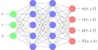
Figure 1: Diagram of the PINN used.

2 Methods

2.1 Rayleigh-Bénard flows and data generation

Rayleigh-Bénard convection consists of a planar horizontal layer of fluid that is heated from below with respect to gravity. If density fluctuations are small, the Boussinesq approximation may be employed and the fluid can be described in terms of an incompressible velocity field plus a temperature field. Taking $\bm{u}=(u,v)$ to be the horizontal and vertical components of the velocity field, respectively, $T$ the temperature and $p$ the pressure, in a 2D geometry and with the average temperature set to zero and the density to unity the equations take the form

$$\partial_{t}\bm{u}+(\bm{u}\cdot\mathbf{\nabla})\bm{u}=-\mathbf{\nabla}p+\nu\nabla^{2}\bm{u}-\beta Tg\hat{z},$$ (1)

$$\frac{\partial T}{\partial t}+\bm{u}\cdot\mathbf{\nabla}T=\kappa\nabla^{2}T,$$ (2)

where $\beta$ is the thermal expansion coefficient of the fluid, $\nu$ is its kinematic viscosity, $\kappa$ its thermal conductivity and $g\hat{z}$ the acceleration due to gravity. The domain is $L_{x}$ wide and $L_{z}$ tall and has periodic boundary conditions in the horizontal direction $\hat{x}$. At the top and bottom boundaries, the boundary conditions are

$$\begin{gathered}T(z=0)=T_{d},\qquad T(z=L_{z})=-T_{d},\\ \bm{u}(z=0)=\bm{u}(z=L_{z})=0.\\ \end{gathered}$$ (3)

where $T_{d}>0$. The characteristic velocity scale is given by $u_{0}=\sqrt{gL_{z}\beta 2T_{d}}$ and the turnover time by $\tau_{0}=2L_{z}/u_{0}$. Several dimensionless numbers can be used to describe Rayleigh-Bénard flows. The Rayleigh number gives a measure of the ratio between buoyant and viscous forces and is given by

$$\rm{Ra}=g\beta\frac{2T_{d}L_{z}^{3}}{\nu\kappa}.$$ (4)

The Prandtl number is the ratio between momentum diffusivity and thermal diffusivity, namely

$$\Pr=\frac{\nu}{\kappa}.$$ (5)

The Nusselt number measures the ratio of heat transfer due to convection versus that due to conduction and is given by

$$\rm{Nu}=\frac{\langle vT-\kappa\partial_{z}T\rangle}{\kappa 2T_{d}/L_{z}},$$ (6)

where $\langle.\rangle$ indicate the ensemble average over the whole domain. Finally, as an estimate of the size of the smallest scales of the system we define the Kolmogorov length scale $\eta_{\kappa}=(\nu^{3}/\epsilon)^{1/4},$ where $\epsilon=(\nu\kappa^{2}/L^{4}_{z})(\rm{Nu}-1)\rm{Ra}$ is the average rate of energy dissipation siggia_high_1994 .

The reference, or ground-truth, flow of our numerical experiments was produced by evolving Eqs. (1)-(2) using a Lattice-Boltzmann method at two different Rayleigh numbers, $\rm{Ra}_{1}=7.2\times 10^{7}$ and $\rm{Ra}_{2}=36.3\times 10^{7}$. The reference flows are denoted by variables $u^{r}$, $v^{r}$, $p^{r}$, and $T^{r}$. Details on the numerical method can be found in agasthya_reconstructing_2022 .

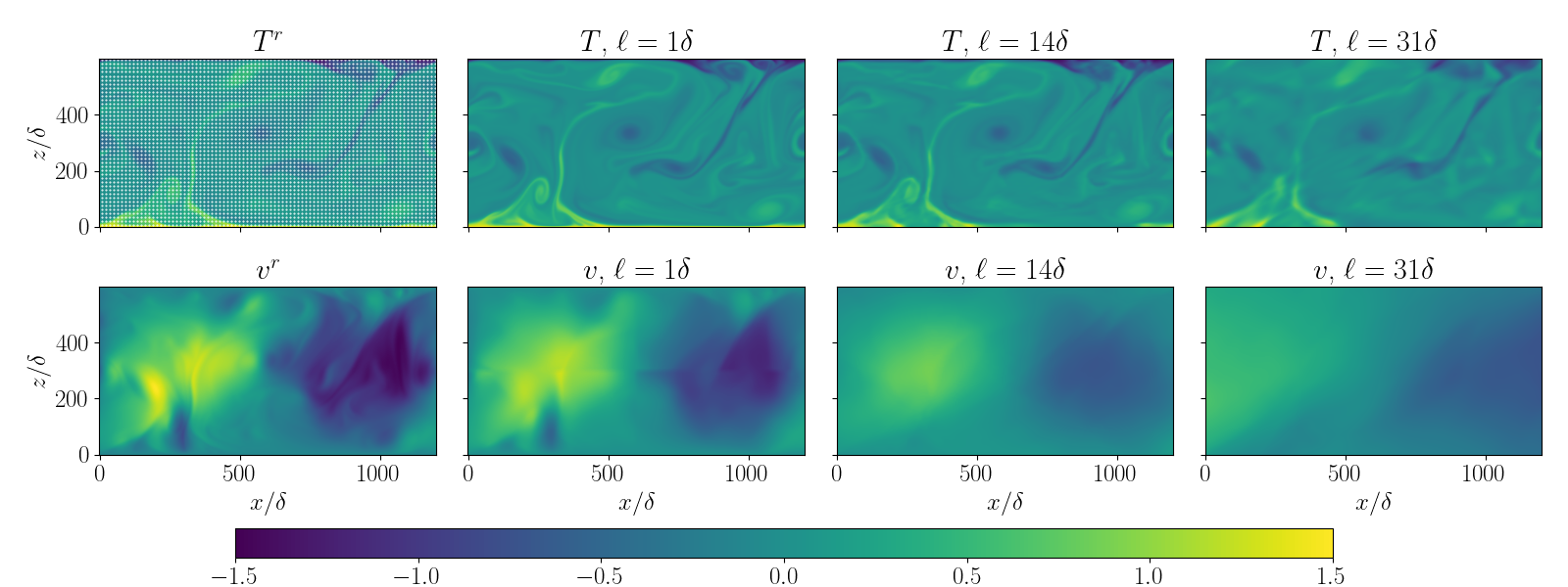
Figure 2: Visualizations of temperature (top) and vertical velocity (bottom) for the flow with $\rm{Ra}_{2}$. The left column shows the reference data, the other three columns show the reconstructions obatined with $\ell/\delta=1$, $14$ and $31$. The locations of the measuring probes (corresponding to the case with $\ell=14\delta$) are marked with white dots on top of $T^{r}$. All visualizations share the same colorbar.

In the first case $L_{x}=864\delta$, $L_{z}=432\delta$, $T_{d}=2.5T_{0}$, and $u_{0}=1.31U_{0}$, while in the second case $L_{x}=1200\delta$, $L_{z}=600\delta$, $T_{d}=1.5T_{0}$, and $u_{0}=2.12U_{0}$. In both cases $\nu=6.67\times 10^{-4}$, $\Pr=1$, $\delta=1$, $T_{0}=1/100$, $U_{0}=1/100$, and $\eta_{\kappa}\approx 2\delta$. In the first case $\rm{Nu}\approx 25$, while in the second case $\rm{Nu}\approx 39$. The flows were first allowed to reach a statistically stationary state and then data was extracted on a equally spaced rectangular grid of separation distance $\ell\in[1:31]\delta$ at specific time intervals. In the first case, data was extracted over 8 separate time windows 11 snapshots long at a sampling rate of $164/\tau_{0}$. In the second case, data was extracted over 10 separated time windows also 11 snapshots long but at a sampling rate of $1130/\tau_{0}$, as this flow contains faster scales than the other one. Data was extracted over the whole spatial domain, except for the case with $\ell=1$ at $\rm{Ra}_{2}$, where the domain was split into four quadrants, thus necessitating four PINNs for the reconstruction of the whole domain. Each dataset $\Omega_{d}$ is then identified by the Rayleigh number of the flow, the grid spacing $\ell$, and the temporal window. The sets of collocation points $\Omega_{p}$ where the physics part of the loss function is evaluated (see below) consist of all points where data part are evaluated, i.e. $\Omega_{d}$, plus randomly selected points not necessarily lying on the $\ell$-spaced sampling grid. Note that as no data are used when evaluating the physics part of the loss function, we are not increasing the density of data used. The number of extra collocation points was 0, 0, 1, 2, 3, and 4 for every spatial position in $\Omega_{d}$ for $\ell/\delta=1,7,10,14,22$, and $31$, respectively. To evaluate the PINNs’ performances testing datasets $\Omega_{t}$ consisting of the full fields, i.e., not subsampled in space, were used.

2.2 Flow reconstruction using PINNs

Figure 1 shows a diagram of the PINN used in our experiments. The PINN takes coordinates $(x,z,t)$ as input and outputs fields $(u,v,p,T)$ at the specified coordinate. All PINNs presented here are five layers deep, have 100 hidden units in each layer and use ELU as activation functions. The loss function used to train them has the form

$$L=L_{d}+\lambda L_{p},$$

with the contribution given by the measured data is given by

$$L_{d}=\frac{1}{N(\Omega_{d})T^{2}_{0}}\sum_{j\in\Omega_{d}}|T(x_{j},z_{j},t_{j})-T^{r}_{j}|^{2},$$

and the one given by the imposition of the correct equations of motion by:

$$L_{p}=\frac{\delta^{2}}{N(\Omega_{p})}\sum_{j\in\Omega_{p}} \left(\lambda_{u}U^{-4}_{0}f_{u}+\lambda_{T}T^{-2}_{0}U^{-2}_{0}f_{T}+\right.$$

$$\left.\lambda_{i}U^{-2}_{0}f_{i}\right),$$

with

$$f_{u}=|\partial_{t}\bm{u}+(\bm{u}\cdot\mathbf{\nabla})\bm{u}+\mathbf{\nabla}p-\nu\nabla^{2}\bm{u}+\beta Tg\hat{z}|^{2},$$

$$f_{T}=|\partial_{t}T+\bm{u}\cdot\mathbf{\nabla}T-\kappa\nabla^{2}T|^{2},$$

and

$$f_{i}=|\nabla\cdot\bm{u}|^{2},$$

and where $\lambda$, $\lambda_{u}$, $\lambda_{T}$ and $\lambda_{i}$ are extra hyperparameters set fixed to $10^{5}$, $1$, $10^{-1}$ and $10^{3}$, respectively, throughout. The subsets of points $\Omega_{d}$ and $\Omega_{p}$ where the summations are evaluated are explained in the section above, $N(\Omega_{d})$ and $N(\Omega_{p})$ denote the number of point in the respective datasets. The PINNs were trained using the Adam algorithm with a learning rate of $10^{-4}$ for 60000 epochs.

2.3 Flow reconstruction using Nudging

Nudging is an equation-informed data assimilation tool, using the evolution of the Navier-Stokes equations (1) supplemented by a Newton relaxation term proportional to $\alpha(T_{(}x_{j},z_{j},t_{j})^{r}-T)$ in the temperature evolution. The resulting equations take the form

$$\partial_{t}\bm{u}+(\bm{u}\cdot\mathbf{\nabla})\bm{u}=-\mathbf{\nabla}p+\nu\nabla^{2}\bm{u}-\beta Tg\hat{z},$$ (7)

$$\frac{\partial T}{\partial t}+\bm{u}\cdot\mathbf{\nabla}T=\kappa\nabla^{2}T-\alpha\mathcal{I}(T^{r}-T),$$

where $\alpha$ is the amplitude of the nudging term and has units of frequency and $\mathcal{I}$ is a filtering operator equal to 1 where the data is available, i.e. the measuring probes, and zero otherwise. The idea in nudging is to force the equation of motion to “follow” the available information where it is available and leave the equations of motion to refill the gaps in the whole space-time domain. For further details about the optimal selection for the nudging parameter $\alpha$ and how to interpolate in time and space the supplied data see agasthya_reconstructing_2022 . In contrast with PINNs, Nudging naturally enforces all physical constraints everywhere, at the cost of evolving the partial differential equations on the entire domain.

2.4 Error assessment

In order to assess the reconstructions obtained, we define the point-to-point error field for temperature and velocity as:

$$T_{\Delta}(\bm{r},t)=T^{r}(\bm{r},t)-T(\bm{r},t)\mathchar 24635\relax\;$$

$$v_{\Delta}(\bm{r},t)=v^{r}(\bm{r},t)-v(\bm{r},t).$$ (8)

Global normalized errors are then given by

$$\Delta_{T}=\frac{\langle T_{\Delta}^{2}(\bm{r},t)\rangle}{\langle T^{2}(\bm{r},t)\rangle}\mathchar 24635\relax\;\qquad\Delta_{v}=\frac{\langle v_{\Delta}^{2}(\bm{r},t)\rangle}{\langle v^{2}(\bm{r},t)\rangle},$$ (9)

where $\langle\cdot\rangle$ indicates the average over the entire domain. It is important to stress that no information on the temperature at the boundary was provided (similarly to what implemented for nudging).

The scale-by-scale analysis is performed by analyzing the energy spectra:

$$E_{f}(k)=\langle|\hat{f}(k,z_{0},t)|^{2}\rangle_{t},$$ (10)

where $f$ is the field studied (either $v$, $v_{\Delta}$, $T$, or $T_{\Delta}$), $\hat{f}(k,z_{0},t)$ are the Fourier coefficients of $f$ calculated along the horizontal direction at position $z_{0}=L_{z}/2$ and time $t$, and $\langle,\rangle_{t}$ denotes the time average.

3 Results

Figure 2 shows visualizations of the reference temperature $T^{r}$ and vertical velocity $v^{r}$ of the flow with $\rm{Ra}_{2}$ at a given time and their PINN-reconstructed counterparts, $T$ and $v$, for three reconstructions, one performed with $\ell/\delta=1$, one with $\ell/\delta=14$ and one with $\ell/\delta=31$. The location of the temperature measuring probes (corresponding to the $\ell/\delta=14$ case) are marked with white dots. These visualizations not only show the characteristics of the flow, but also give a qualitative glimpse into the overall results: PINNs are able to reconstruct/infer the velocity field using only temperature information, even at high Rayleigh number, but with clear difficulties to capture small-scales fluctuations, as shown by the blurred velocity configurations (middle and right bottom panels). To further stress this point, we show the horizontal profile at $z_{0}=300\delta$ in Fig. 3 with three different $\ell/\delta=1,14,31$ for temperature (top), and velocity (bottom). As seen, the temperature reconstruction almost overlaps with the reference data for all cases, except the one with $\ell/\delta=31$. The reconstructed velocity field, on the other hand, is able to correctly match the large scale structure of the reference flow, but is missing smaller scale features. Furthermore, the effects of not enforcing periodic boundary conditions along the horizontal direction can be clearly seen in the $\ell/\delta=31$ case.

To put matters into quantitative terms, in Fig. 4 we show $\Delta_{T}$ and $\Delta_{v}$ obtained for the different $\ell/\delta$ and the two Rayleigh numbers. The figures also show the results obtained via Nudging presented in agasthya_reconstructing_2022 . As shown on the top panel of Fig. 4 for the case of the temperature field, PINNs and Nudging perform similarly. On the other hand, concerning the most interesting -and difficult- question of reconstructing the velocity field, in the bottom panel we show that PINNs outperform Nudging when the supplied temperature is dense enough in space $\delta/\ell\sim 1$, while it is comparable with Nudging for sparse data, $\delta/\ell<8\times 10^{-2}$.

In Fig. 5 (top) we show the temperature spectra at $y_{0}=300\delta$ of the reference flow and of the reconstructions obtained with $\ell=1\delta$, $14\delta$, and $31\delta$ for the high Rayleigh number case, while in the bottom panel we show the the spectra of the reference field superimposed with the spectra of the error $T_{\Delta}$. A Hanning window was applied to the reconstructed fields to cure any effects of non-periodicity. The vertical dash-dotted red line marks where $k\delta=14$ and the veritcal dotted green line where $k\delta=31$. As expected from the previous analysis, the overall errors are small and mostly concentrated in the small scales, although in the $\ell=14\delta$ and $31\delta$ cases, these are still bigger than the scale set by $\ell$. Figure 6 shows the corresponding spectra of the vertical velocity, with the addition of the result obtained via nudging agasthya_reconstructing_2022 for $\ell/\delta=14$. Here, only in the case with $\ell/\delta=1$ the PINN produces a physically meaningful energy spectrum, while the spectra obtained via nudging is very similar to the reference one. In accordance with Figs. 2 and 3, the cases with higher $\ell/\delta$ can only properly reconstruct the position and shape of the largest structures of the flow, but fail to produce the small-scale structures observed at these Rayleigh numbers. The energy spectra of the reconstruction thus decay very rapidly.

Finally, in Fig. 7(a) and (b) we show the probability density functions (excluding the regions close to the walls) of temperature and vertical velocity, respectively for the case with $\rm{Ra}_{2}$. As expected, temperature statistics are well reproduced for all $\ell$ presented, while velocity statistics are only close to accurate when $\ell=1$, otherwise the probability density function start resembling a Gaussian.

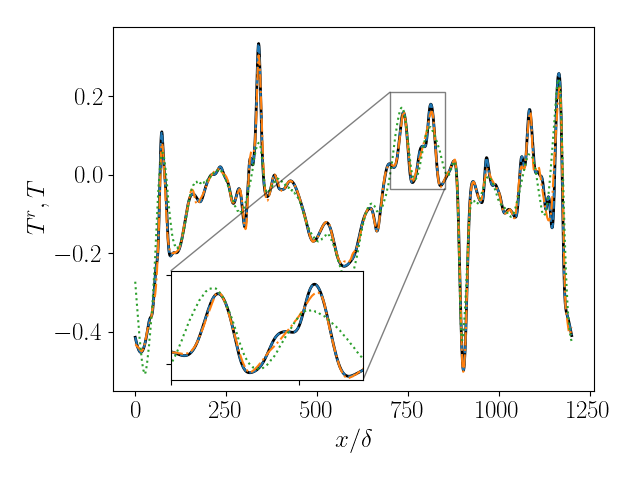
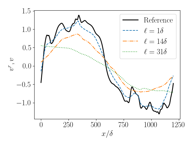
Figure 3: Temperature (top) and velocity (bottom) profiles for the case with $\rm{Ra}_{2}$. The reconstructions shown were obtained using $\ell/\delta=1$, 14, and 31. Both figures share the same legend.

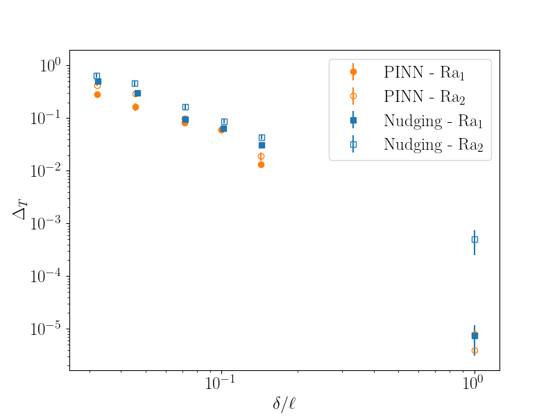
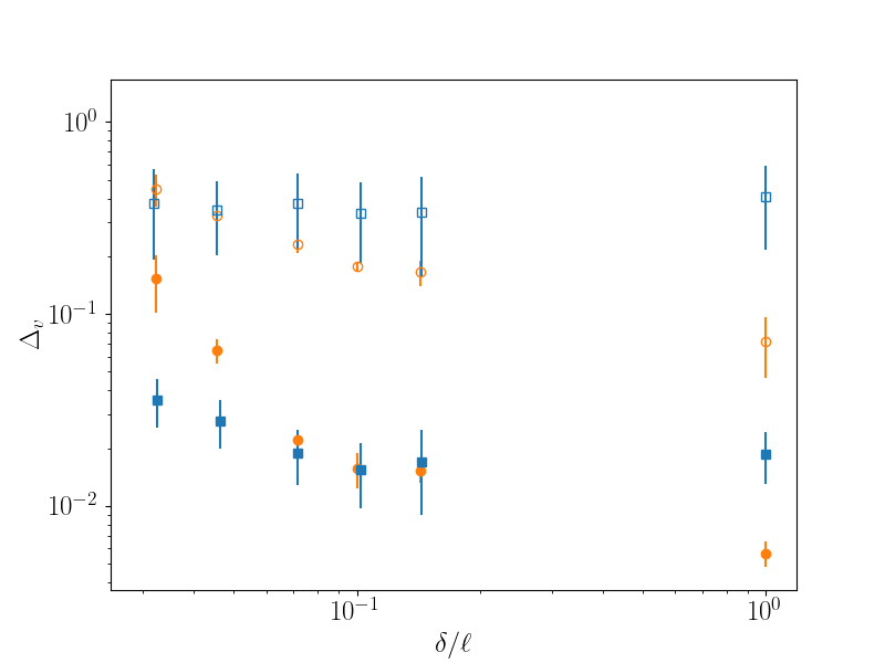
Figure 4: Global temperature errors $\Delta_{T}$ (top) and global velocity errors $\Delta_{v}$ (bottom) as a function of $\delta/\ell$. Full markers denote the results for the case with $\rm{Ra}_{1}$, while empty markers denote the case with $\rm{Ra}_{2}$. The orange circular markers are the results obtained with PINNs, while the blue square markers are for the results obtained via nudging (extracted from agasthya_reconstructing_2022 ). Both figures share the same legend.

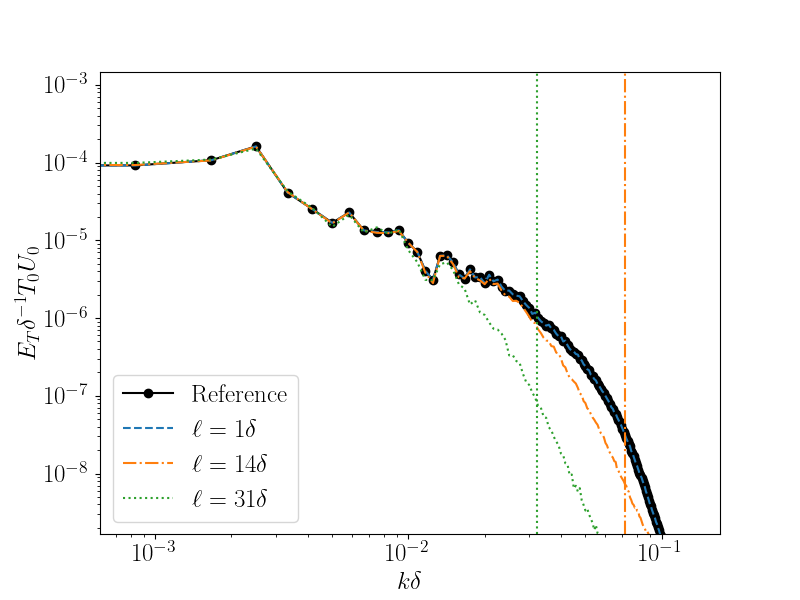
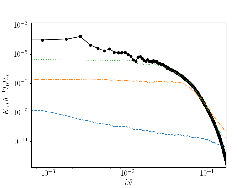
Figure 5: Top: temperature spectra for the reference flow at $\rm{Ra}_{2}$ and the spectra reconstructed fields obtained with $\ell/\delta=1$, 14, and 31. The vertical dash-dotted red line marks where $k\delta=14$, while the vertical dotted green line where $k\delta=31$. Bottom: temperature spectra for the reference flow at $\rm{Ra}_{2}$ and the spectra of the temperature error fields obtained with $\ell/\delta=1$, 14, and 31. Both figures share the same legend.

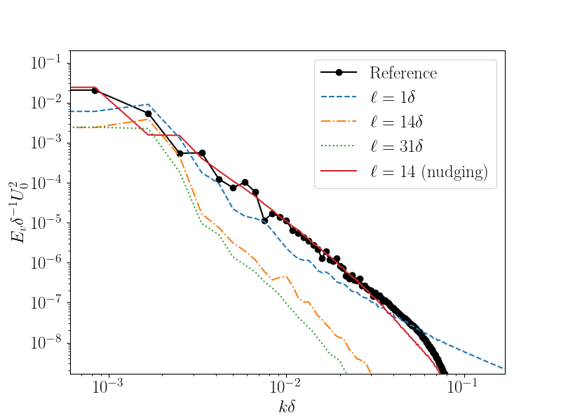
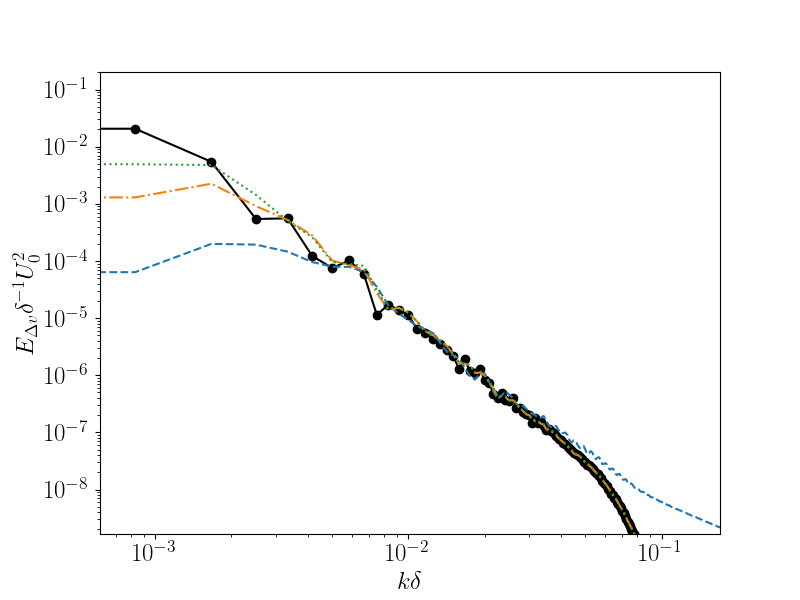
Figure 6: Top: vertical velocity spectra for the reference flow at $\rm{Ra}_{2}$ and the spectra reconstructed fields obtained with $\ell/\delta=1$, 14, and 31. The solid red line corresponds to the obtained via nudging agasthya_reconstructing_2022 . Bottom: vertical velocity spectra for the reference flow at $\rm{Ra}_{2}$ and the spectra of the vertical velocity error fields obtained with $\ell/\delta=1$, 14, and 31. Both figures share the same legend.

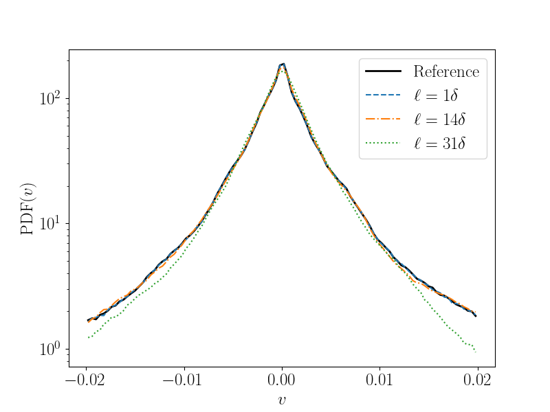
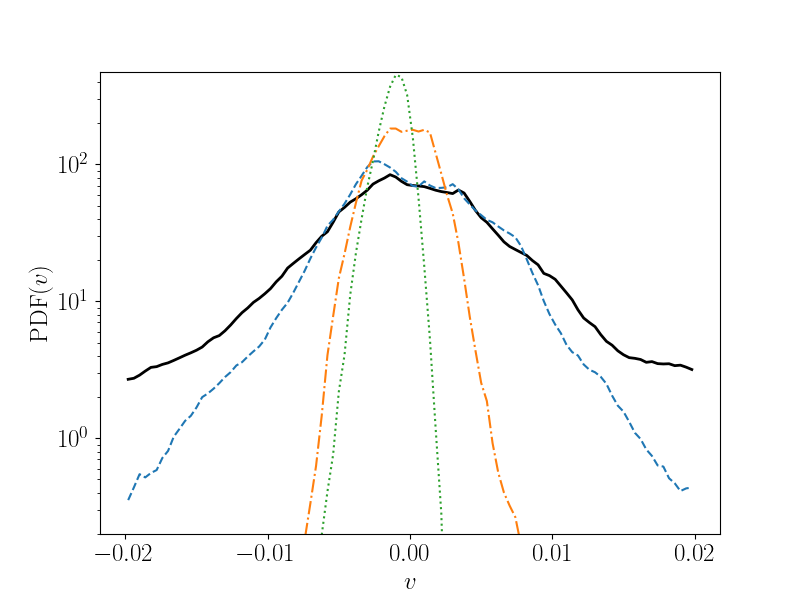
Figure 7: Temperature (top) and vertical velocity (bottom) probability density functions for the reference flow at $\rm{Ra}_{2}$ and for the reconstruction performed with $\ell/\delta=1$, 14, and 31. Both figures share the same legend.

4 Conclusions

Machine and deep learning techniques are becoming well-established tools in the Data Assimilation world. We show that it is possible to reconstruct Rayleigh-Bénard velocity fields having access only to time-resolved point-wise temperature measurements using PINNs. We investigate two different Rayleigh numbers at $7.2\times 10^{7}$ and $3.6\times 10^{8}$. In order to assess the accuracy of PINNs we compare the results against a baseline given by Nudging agasthya_reconstructing_2022 . PINNs achieve an accuracy comparable to Nudging for the smallest Rayleigh number and a better accuracy for highest Rayleigh case when the temperature data are supplied at high spatial frequencies. On the other hand, when temperature is too sparse, PINNs fail to produce meaningful results, while Nudging still produces physically valid solutions. We interpret this as a lack to enforce the correct physical constraints when data are not dense enough. As seen in other works clark_di_leoni_reconstructing_2022 ; cuomo_scientific_2022 , PINNs can struggle with high-frequency components, a major problem in multi-scale turbulent data where information is key also at small-scales and high-frequencies. It is important to remark that while the results presented can be considered promising, we do not claim they are optimal under any criteria, better results may be obtained with a different choice of hyperparameters, a slight modifications to the architecture du_VarPINN2022 , by enforcing periodicity in the horizontal direction via Fourier features tancik_fourier_2020 , or by splitting the domain into smaller subsections karniadakis_extended_2020 . It is out of the scope of this work to perform an exhaustive and meaningful hyperparameter scan. This work can be considered another exploratory attempt to systematic assess ML tools for reconstructing multi-scale turbulent fields, imposing physics constraints. Our intention here is to stress the importance to compare with other baselines (here Nudging is used), the need -in future works- to explore a wider range of Rayleigh (here limited to $[10^{7}:10^{8}]$) and to jump to full $3d+1$ space-time domains, the need to distinguish point-based reconstructions (here assessed in term of $L_{2}$ norm, and spectral errors) from statistical reconstruction (here assessed with spectral and probability density functions). As far as this study shows, when data are sparse, PINNs performance worsens. Contrary to Nudging, the obtained reconstructed fields not only have a high point-to-point error but also have incorrect energy spectra and statistics.

Declarations

The datasets generated during and/or analysed during the current study are available from the corresponding author on reasonable request.

L.A. and P.C. conceived and carried out the numerical experiments, and analyzed the results. All authors worked on developing the main idea, discussed the results and contributed to the final manuscript.

This project has received partial funding from the European Research Council (ERC) under the European Union’s Horizon 2020 research and innovation programme (Grant Agreement No. 882340)).

References

- (1) D. L. Hartmann, L. A. Moy, and Q. Fu, “Tropical convection and the energy balance at the top of the atmosphere,” Journal of Climate, vol. 14, no. 24, pp. 4495–4511, 2001.
- (2) K. Suselj, M. J. Kurowski, and J. Teixeira, “A unified eddy-diffusivity/mass-flux approach for modeling atmospheric convection,” Journal of the Atmospheric Sciences, vol. 76, no. 8, pp. 2505–2537, 2019.
- (3) K. Våge, L. Papritz, L. Håvik, M. A. Spall, and G. W. K. Moore, “Ocean convection linked to the recent ice edge retreat along east greenland,” Nature communications, vol. 9, no. 1, pp. 1–8, 2018.
- (4) M. Kronbichler, T. Heister, and W. Bangerth, “High accuracy mantle convection simulation through modern numerical methods,” Geophysical Journal International, vol. 191, no. 1, pp. 12–29, 2012.
- (5) A. Brent, V. R. Voller, and K. Reid, “Enthalpy-porosity technique for modeling convection-diffusion phase change: application to the melting of a pure metal,” Numerical Heat Transfer, Part A Applications, vol. 13, no. 3, pp. 297–318, 1988.
- (6) G. Ahlers, S. Grossmann, and D. Lohse, “Heat transfer and large scale dynamics in turbulent rayleigh-bénard convection,” Rev. Mod. Phys., vol. 81, pp. 503–537, Apr 2009.
- (7) J. Charney, M. Halem, and R. Jastrow, “Use of incomplete historical data to infer the present state of the atmosphere,” J. Atmos. Sci., vol. 26, pp. 1160–1163, 1969.
- (8) M. Ghil, B. Shkoller, and V. Yangarber, “A Balanced Diagnostic System Compatible with a Barotropic Prognostic Model,” Monthly Weather Review, vol. 105, pp. 1223–1238, Oct. 1977. Publisher: American Meteorological Society Section: Monthly Weather Review.
- (9) M. Ghil, M. Halem, and R. Atlas, “Time-Continuous Assimilation of Remote-Sounding Data and Its Effect an Weather Forecasting,” Monthly Weather Review, vol. 107, pp. 140–171, Feb. 1979. Publisher: American Meteorological Society Section: Monthly Weather Review.
- (10) A. Farhat, E. Lunasin, and E. Titi, “On the charney conjecture of data assimilation employing temperature measurements alone: The paradigm of 3d planetary geostrophic model,” Mathematics of Climate and Weather Forecasting, vol. 2, 08 2016.
- (11) M. U. Altaf, E. S. Titi, T. Gebrael, O. M. Knio, L. Zhao, M. F. McCabe, and I. Hoteit, “Downscaling the 2D Bénard convection equations using continuous data assimilation,” Computational Geosciences, vol. 21, pp. 393–410, June 2017.
- (12) M. A. E. R. Hammoud, E. S. Titi, I. Hoteit, and O. Knio, “CDAnet: A Physics-Informed Deep Neural Network for Downscaling Fluid Flows,” Journal of Advances in Modeling Earth Systems, vol. 14, no. 12, p. e2022MS003051, 2022. _eprint: https://onlinelibrary.wiley.com/doi/pdf/10.1029/2022MS003051.
- (13) A. Farhat, N. E. Glatt-Holtz, V. R. Martinez, S. A. McQuarrie, and J. P. Whitehead, “Data assimilation in large prandtl rayleigh–benard convection from thermal measurements,” SIAM Journal on Applied Dynamical Systems, vol. 19, no. 1, pp. 510–540, 2020.
- (14) L. Agasthya, P. Clark Di Leoni, and L. Biferale, “Reconstructing Rayleigh–Bénard flows out of temperature-only measurements using nudging,” Physics of Fluids, vol. 34, p. 015128, Jan. 2022. Publisher: American Institute of Physics.
- (15) E. Kalnay, Atmospheric Modeling, Data Assimilation and Predictability. Cambridge University Press, 2003.
- (16) P. Bauer, A. Thorpe, and G. Brunet, “The quiet revolution of numerical weather prediction,” Nature, vol. 525, no. 7567, pp. 47–55, 2015.
- (17) S. Lakshmivarahan and J. M. Lewis, “Nudging methods: A critical overview,” in Data Assimilation for Atmospheric, Oceanic and Hydrologic Applications (Vol. II), pp. 27–57, Springer, Berlin, Heidelberg, 2013.
- (18) M. Buzzicotti and P. Clark Di Leoni, “Synchronizing subgrid scale models of turbulence to data,” Physics of Fluids, vol. 32, no. 12, p. 125116, 2020.
- (19) P. Clark Di Leoni, A. Mazzino, and L. Biferale, “Synchronization to Big Data: Nudging the Navier-Stokes Equations for Data Assimilation of Turbulent Flows,” Physical Review X, vol. 10, p. 011023, Feb. 2020. Publisher: American Physical Society.
- (20) M. Raissi, P. Perdikaris, and G. E. Karniadakis, “Physics-informed neural networks: A deep learning framework for solving forward and inverse problems involving nonlinear partial differential equations,” Journal of Computational Physics, vol. 378, pp. 686–707, Feb. 2019.
- (21) M. Raissi, A. Yazdani, and G. E. Karniadakis, “Hidden fluid mechanics: Learning velocity and pressure fields from flow visualizations,” Science, vol. 367, pp. 1026–1030, Feb. 2020. Publisher: American Association for the Advancement of Science Section: Report.
- (22) K. Shukla, P. Clark Di Leoni, J. Blackshire, D. Sparkman, and G. E. Karniadakis, “Physics-Informed Neural Network for Ultrasound Nondestructive Quantification of Surface Breaking Cracks,” Journal of Nondestructive Evaluation, vol. 39, p. 61, Aug. 2020.
- (23) S. Cai, Z. Wang, F. Fuest, Y. J. Jeon, C. Gray, and G. E. Karniadakis, “Flow over an espresso cup: inferring 3-D velocity and pressure fields from tomographic background oriented Schlieren via physics-informed neural networks,” Journal of Fluid Mechanics, vol. 915, May 2021. Publisher: Cambridge University Press.
- (24) H. Wang, Y. Liu, and S. Wang, “Dense velocity reconstruction from particle image velocimetry/particle tracking velocimetry using a physics-informed neural network,” Physics of Fluids, vol. 34, p. 017116, Jan. 2022. Publisher: American Institute of Physics.
- (25) Y. Du, M. Wang, and T. A. Zaki, “State estimation in minimal turbulent channel flow: A comparative study of 4DVar and PINN,” International Journal of Heat and Fluid Flow, 2022.
- (26) P. Clark Di Leoni, K. Agarwal, T. Zaki, C. Meneveau, and J. Katz, “Reconstructing velocity and pressure from sparse noisy particle tracks using Physics-Informed Neural Networks,” Oct. 2022. arXiv:2210.04849 [physics].
- (27) S. Angriman, P. Cobelli, P. Mininni, M. Obligado, and P. Clark Di Leoni, “Generation of Turbulent States using Physics-Informed Neural Networks,” Sept. 2022. arXiv:2209.04285 [physics].
- (28) S. Cai, Z. Mao, Z. Wang, M. Yin, and G. E. Karniadakis, “Physics-informed neural networks (PINNs) for fluid mechanics: a review,” Acta Mechanica Sinica, vol. 37, pp. 1727–1738, Dec. 2021.
- (29) S. Cuomo, V. S. Di Cola, F. Giampaolo, G. Rozza, M. Raissi, and F. Piccialli, “Scientific Machine Learning Through Physics–Informed Neural Networks: Where we are and What’s Next,” Journal of Scientific Computing, vol. 92, p. 88, July 2022.
- (30) E. D. Siggia, “High Rayleigh Number Convection,” Annual Review of Fluid Mechanics, vol. 26, no. 1, pp. 137–168, 1994. _eprint: https://doi.org/10.1146/annurev.fl.26.010194.001033.
- (31) M. Tancik, P. P. Srinivasan, B. Mildenhall, S. Fridovich-Keil, N. Raghavan, U. Singhal, R. Ramamoorthi, J. T. Barron, and R. Ng, “Fourier Features Let Networks Learn High Frequency Functions in Low Dimensional Domains,” arXiv:2006.10739 [cs], June 2020. arXiv: 2006.10739.
- (32) A. D. J. . G. E. Karniadakis, “Extended Physics-Informed Neural Networks (XPINNs): A Generalized Space-Time Domain Decomposition Based Deep Learning Framework for Nonlinear Partial Differential Equations,” Communications in Computational Physics, vol. 28, pp. 2002–2041, June 2020.