Prony-Based Super-Resolution Phase Retrieval of Sparse, Multivariate Signals

Abstract

Phase retrieval consists in the recovery of an unknown signal from phaseless measurements of its usually complex-valued Fourier transform. Without further assumptions, this problem is notorious to be severe ill posed such that the recovery of the true signal is nearly impossible. In certain applications like crystallography, speckle imaging in astronomy, or blind channel estimation in communications, the unknown signal has a specific, sparse structure. In this paper, we exploit these sparse structure to recover the unknown signal uniquely up to inevitable ambiguities as global phase shifts, transitions, and conjugated reflections. Although using a constructive proof essentially based on Prony’s method, our focus lies on the derivation of a recovery guarantee for multivariate signals using an adaptive sampling scheme. Instead of sampling the entire multivariate Fourier intensity, we only employ Fourier samples along certain adaptively chosen lines. For bivariate signals, an analogous result can be established for samples in generic directions. The number of samples here scales quadratically to the sparsity level of the unknown signal.

1 Introduction

Phase retrieval is one of the major challenges in many imaging tasks in physics and engineering. For instance, phase retrieval is an essential component of the imaging techniques: ptychography [16], crystallography [17], speckle imaging [15], diffraction tomography [9]. Although there are many different problem formulations summarized as “phase retrieval”, the main task consists in the recovery of an image or signal form the magnitudes of usually complex-valued measurements. If we think at the application in optics, the measurements often correspond to the magnitudes of the Fourier or Fresnel transform. Although the Fourier and Fresnel transform are invertible, the loss of the phase turns the imaging task into an severe ill-posed inverse problem. The central challenge is here the strong ambiguousness, which has been studied for the continuous as well as for the discrete setting, see for instance [5, 10, 11]. To overcome the ambiguousness, different a priori informations like support constraints or non-negativity as well as additional measurements have been studied [13, 14, 8, 3, 4].

In this paper, we are interested in the recovery of multivariate, sparse signals, which are modeled as complex measure

$$\mu\coloneqq\sum_{n=1}^{N}c_{n}\,\nu(\cdot-T_{n}),$$

where $\nu$ is a known structure. Choosing $\nu$ as Dirac measure, we obtain point measures or spike functions. But other choices like Gaussians are reasonable too and lead to more regular functions. We here consider the Fourier phase retrieval problem, meaning that we want to recover $c_{n}$ and $T_{n}$ from samples of the Fourier intensity—the magnitude of the Fourier transform—of $\mu$. Our focus lies on the derivation of uniqueness guarantees, i.e. on assumptions allowing the determination of $c_{n}$ and $T_{n}$ up to unavoidable ambiguities. Since the transitions $T_{n}$ may lie on a continuous domain, our problem can be interpreted as super-resolution phase retrieval [1]. This kind of problem arises in applications like crystallography [17], speckle imaging in astronomy [15] as well as in blind channel estimation in communication [2].

Methodology and Relation to the Literature

To show that phase retrieval of sparse, multivariate signals is possible in principle, we rely on the Prony-based techniques in [6], where super-resolution phase retrieval is studied for univariate signals. For the generalization to multivariate signals, we employ an adaptive sampling strategy, where the Fourier intensity of the unknown signal is measured along adaptively chosen or along generic lines. This sampling method traces back to [19], where the recovery of sparse signals from their (complex-valued) Fourier transform is studied. Our main idea is to use the specific sampling setup to reduce the multivariate phase retrieval problem into a series of univariate problems, to solve these univariate instances as in [6], and to combine the extracted informations to solve the multivariate instance. The considered super-resolution phase retrieval problem has also been studied in [1], where a greedy-like algorithm is proposed to solve the problem numerically. In difference to [1], where the entire Fourier domain is sampled, we show that the unknown $D$-variate signal is completely determined by $\mathcal{O}(N^{2})$ measurements on $2D-1$ lines, where $N$ denotes the sparsity level.

Contribution

The contribution of this paper is the derivation of a recovery guarantee for super-resolution phase retrieval of multivariate signals. The main theorem shows that, under mild assumptions like collision-freeness, the unknown signal is completely determined by equispaced samples on a few lines. All in all, we here require $\mathcal{O}(DN^{2})$ samples of the Fourier intensity to recover a $D$-variate signal composed of $N$ components. This shows that, at least theoretically, it is enough to use a space sampling setup to recover a sparse signal. Although the proofs are constructive, the focus lies on the theoretical uniqueness guarantee since the applied Prony method is known to be unstable for noisy measurements.

Outline

Before considering the super-resolution phase retrieval problem, we briefly introduce the needed concepts like the Fourier transform of measures and Prony’s method in § 2. In § 3, we define the considered problem in more details and discuss the unavoidable ambiguities. Section 4 is devoted to the univariate sparse phase retrieval problem, which we generalize to the multivariate setting in § 5. The numerical simulation in § 6 show that the constructive proofs can be implemented to recover the unknown signal at least in the noise-free setting. A final discussion is given in § 7.

2 Preleminaries

2.1 Fourier Transform of Measures

Subsequently, the unknown signals are characterized as complex measures. For this, let $\operatorname{\mathcal{B}}(\bbbr^{D})$ denote the Borel $\sigma$-algebra of the Euclidean space $\bbbr^{D}$, and $\operatorname{\mathcal{M}}(\bbbr^{D})$ the space of all regular, finite, complex measures. Every considered signal is then interpreted as complex-valued mapping $\mu\colon\operatorname{\mathcal{B}}(\bbbr^{D})\to\bbbc$ with $\mu\in\operatorname{\mathcal{M}}(\bbbr^{D})$. Recall that $\operatorname{\mathcal{M}}(\bbbr^{D})$ is the dual space of $C_{0}(\bbbr^{D})$, which consists of all continuous functions $\phi\colon\bbbr^{D}\to\bbbc$ where $\phi(x)$ vanishes for $\lVert x\rVert\to\infty$. Every measure $\mu\in\operatorname{\mathcal{M}}(\bbbr^{D})$ hence defines a continuous, linear mapping via

$$\phi\mapsto\langle\mu,\phi\rangle\coloneqq\int_{\bbbr^{D}}\phi(x)\mathop{}\!\mathrm{d}\mu(x).$$

The convolution of two measures $\mu,\nu\in\operatorname{\mathcal{M}}(\bbbr^{D})$ is indirectly defined as

$$\langle\mu*\nu,\phi\rangle\coloneqq\iint_{\bbbr^{D}\times\bbbr^{D}}\phi(x+y)\mathop{}\!\mathrm{d}\nu(y)\mathop{}\!\mathrm{d}\mu(x),\quad\phi\in C_{0}(\bbbr^{D}).$$

The Fourier transform on $\operatorname{\mathcal{M}}(\bbbr^{D})$ is given by $\operatorname{\mathcal{F}}\colon\operatorname{\mathcal{M}}(\bbbr^{D})\to C_{\mathrm{b}}(\bbbr^{D})$ with

$$\operatorname{\mathcal{F}}[\mu](\omega)\coloneqq\hat{\mu}(\omega)\coloneqq\int_{\bbbr^{D}}\mathrm{e}^{-\mathrm{i}\langle\omega,x\rangle}\mathop{}\!\mathrm{d}\mu(x),\quad\omega\in\bbbr^{D},$$

where $C_{\mathrm{b}}(\bbbr^{D})$ consists of all bounded, continuous functions on $\bbbr^{D}$. Notice that $\operatorname{\mathcal{F}}$ is continuous and injective. Further, the Fourier convolution theorem states

$$\operatorname{\mathcal{F}}[\mu*\nu]=\hat{\mu}\hat{\nu}.$$

2.2 Prony’s Method

The Fourier intensities of a sparse signal on $\bbbr$ are essentially given by a non-negative exponential sum $E\colon\bbbr\to\bbbr$ of the form

$$E(\omega)\coloneqq\sum_{\ell=-L}^{L}\gamma_{\ell}\,\mathrm{e}^{-\mathrm{i}\omega\tau_{\ell}}=\gamma_{0}+\sum_{\ell=1}^{L}\bigl{(}\gamma_{\ell}\,\mathrm{e}^{-\mathrm{i}\omega\tau_{\ell}}+\bar{\gamma}_{\ell}\,\mathrm{e}^{\mathrm{i}\omega\tau_{\ell}}\bigr{)}$$ (1)

with $\gamma_{\ell}=\bar{\gamma}_{-\ell}\in\bbbc\setminus\{0\}$ and $\tau_{\ell}=-\tau_{-\ell}\in\bbbr$ for $\ell=0,\dots,L$. Note that $\gamma_{0}\in\bbbr\setminus\{0\}$ and $\tau_{0}=0$. For pairwise distinct $\tau_{\ell}$, the parameters $\gamma_{\ell}$ and $\tau_{\ell}$ may be recovered by Prony’s method [21, 12, 20]. In a nutshell, for $h>0$ with $h\tau_{\ell}<\pi$, $\ell=1,\dots,L$, and for $M\geq 4L+1$, we define the Prony polynomial

$$\Lambda(z)\coloneqq\prod_{\ell=-L}^{L}\bigl{(}z-\mathrm{e}^{-\mathrm{i}h\tau_{\ell}}\bigr{)}=\sum_{k=0}^{2L+1}\lambda_{k}\,z^{k},\quad z\in\bbbc,$$ (2)

and observe

$$\sum_{k=0}^{2L+1}\lambda_{k}\,E(h(k+m))=\sum_{\ell=-L}^{L}\gamma_{\ell}\,\mathrm{e}^{-\mathrm{i}hm\tau_{\ell}}\,\Lambda(\mathrm{e}^{-\mathrm{i}h\tau_{\ell}})=0$$

for $m=0,\dots,M-2L-1$. Due to $\lambda_{2L+1}=1$, we may compute the remaining $\lambda_{\ell}$ by solving an equation system, whose solution is, in fact, unique. Knowing $\lambda_{\ell}$, we determine the roots of $\Lambda$ and the frequencies $\tau_{\ell}$. The coefficients $\gamma_{\ell}$ are then given by the over-determined Vandermonde-type system

$$\sum_{\ell=-L}^{L}\gamma_{\ell}\,\mathrm{e}^{-\mathrm{i}hm\tau_{\ell}}=E(hm),\quad m=0,\dots,M.$$ (3)

For our numerical experiments, we use the so-called Approximative Prony Method (APM) by Potts and Tasche [20], which is based on the above consideration but is numerically more stable.

Algorithm 1 (APM, [20])

Input: $L\in\bbbn$, $M\geq 4L+1$, $h>0$ with $h\tau_{\ell}<\pi$, $(E(hm))_{m=0}^{M}$.

1. Compute the right singular vector $(\lambda_{\ell})_{\ell=0}^{2L+1}$ to the smallest singular value of

   $$(E(h(k+m)))_{m,k=0}^{M-2L-1,2L+1}.$$

2. Compute the roots $(z_{\ell})_{\ell=-L}^{L}$ of $\Lambda(z)$ in (2) in order $z_{\ell}=\bar{z}_{-\ell}$.

3. Compute the least-square solution $(\gamma_{\ell})_{\ell=-L}^{L}$ of (3).

4. Set $\tau_{\ell}\coloneqq h^{-1}\arg z_{\ell}$.

Output: $\gamma_{\ell}$, $\tau_{\ell}$, $\ell=-L,\dots,L$.

Instead of the exact number of terms $2L+1$, the method can be applied with an upper estimate for $L$. In this case, $z_{\ell}$ not lying on the unit circle and terms with small $\gamma_{\ell}$ can be neglected.

3 The Phase Retrieval Problem

Originally, phase retrieval means the recovery of an unknown signal only from the intensities of its Fourier transform. In the following, we consider phase retrieval for sparse signals, which are superpositions of finitely many transitions of one known structure. Moreover, signal and structure are modeled as complex measures. Thus, the true signal $\mu\in\operatorname{\mathcal{M}}(\bbbr^{D})$ is a superposition of finitely many transitions $\nu_{T_{n}}\coloneqq\nu(\cdot-T_{n})$ with $T_{n}\in\bbbr^{D}$ and $\nu\in\operatorname{\mathcal{M}}(\bbbr^{D})$. Using the convolution and the Dirac measure $\delta$, the considered phase retrieval problem has the following form: recover the coefficients $c_{n}\in\bbbc\setminus\{0\}$ and the translations $T_{n}\in\bbbr^{D}$ of the structured signal

$$\mu\coloneqq\sum_{n=1}^{N}c_{n}\,\nu_{T_{n}}=\nu*\Bigl{(}\sum_{n=1}^{N}c_{n}\,\delta_{T_{n}}\Bigr{)}$$ (4)

with $\nu\in\operatorname{\mathcal{M}}(\bbbr^{D})$ from samples of its (squared) Fourier intensity

$$\lvert\hat{\mu}(\omega)\rvert^{2}=\lvert\hat{\nu}(\omega)\rvert^{2}\sum_{n=1}^{N}\sum_{k=1}^{N}c_{n}\bar{c}_{k}\,\mathrm{e}^{-\mathrm{i}\langle\omega,T_{n}-T_{k}\rangle}=\lvert\hat{\nu}(\omega)\rvert^{2}\sum_{\ell=-L}^{L}\gamma_{\ell}\,\mathrm{e}^{-\mathrm{i}\langle\omega,\tau_{\ell}\rangle}.$$ (5)

The (indexed) families of translates and coefficients are henceforth denoted by $\mathfrak{T}\coloneqq[T_{1},\dots,T_{N}]$ and $\mathfrak{C}\coloneqq[c_{1},\dots,c_{N}]$, where the index of $c_{n}$ and $T_{n}$ always corresponds to each other. Conceivable structures are the Dirac measure $\delta$, in which case $\mu$ may be interpreted as Dirac signal, or a Gaussian, in which case $\mu$ may be interpreted as ordinary function via its density function. The considered phase retrieval problem is never uniquely solvable.

Lemma 1 (Trivial Ambiguities)

For every $\mu\in\operatorname{\mathcal{M}}(\bbbr^{D})$, global phase shifts, transitions, and conjugated reflections have the same Fourier intensity, i.e.

$$\lvert\hat{\mu}\rvert=\lvert\operatorname{\mathcal{F}}[\mathrm{e}^{\mathrm{i}\alpha}\mu]\rvert=\lvert\operatorname{\mathcal{F}}[\mu(\cdot-x_{0})]\rvert=\lvert\operatorname{\mathcal{F}}[\overline{\mu(-\cdot)}]\rvert,\quad\alpha\in\bbbr,\;x_{0}\in\bbbr^{D}.$$

Since the statement can be established using standard computation rules of the Fourier transform, the proof is omitted. Besides these so-called trivial ambiguities, there may occur further non-trivial ambiguities.

Lemma 2 (Non-Trivial Ambiguities)

Let $\mu=\mu_{1}*\mu_{2}$ be the convolution of $\mu_{1},\mu_{2}\in\operatorname{\mathcal{M}}(\bbbr^{D})$. The signal $\mu_{1}*\overline{\mu_{2}(-\cdot)}$ then has the same Fourier intensity.

The statement immediately follows form the Fourier convolution theorem. As an immediate consequence, we may conjugate and reflect the structure part $\nu$ and the location part $\sum_{n=1}^{N}c_{n}\,\delta_{T_{n}}$ of (4) independently of each other. Therefore, we may only hope to recover $\mu$ up to the following ambiguities.

Definition 1 (Inevitable Ambiguities)

The signal in (4) can only be recovered up to a global phase shift of all coefficients in $\mathfrak{C}$; a global shift of all transitions in $\mathfrak{T}$; and the conjugation of $\mathfrak{C}$ together with the reflection of $\mathfrak{T}$.

In general, the number of non-trivial ambiguities can be immense. For example, under the assumption that the transitions $\mathfrak{T}$ are equispaced, there may exists up to $2^{N-2}$ non-trivial ambiguities [5], which can be characterized as in Lemma 2. To get rid of the non-trivial ambiguities, we have to assume that the transitions $\mathfrak{T}$ are somehow unregular.

Definition 2 (Collision-Freeness)

A family $\mathfrak{T}\coloneqq[T_{1},\dots,T_{N}]\subset\bbbr^{D}$ is called collision-free if the differences $T_{n}-T_{k}$ are pairwise distinct for all $n\neq k$.

4 Sparse Phase Retrieval on the Line

Phase retrieval of structured signals on the line has been well studied [6, 22, 7, 18]. Under certain assumptions, the recovery from equispaced measurements is principally possible.

Theorem 4.1 (Phase Retrieval, [6, Thm 3.1])

Let $\mu$ be of the form (4) with $\hat{\nu}(\omega)\neq 0$, $\omega\in\bbbr$, collision-free $T_{1}<\cdots<T_{N}$, and $\lvert c_{1}\rvert\neq\lvert c_{N}\rvert$. Further, choose $h>0$ such that $h(T_{n}-T_{k})<\pi$ for $n,k$. Then $\mu$ can be uniquely reconstructed from $\lvert\hat{\mu}(hm)\rvert$, $m=0,\dots,2N(N-1)+1$, up to inevitable ambiguities.

The constructive proof leads to a two-step algorithm: First, the parameters $\gamma_{\ell}$ and $\tau_{\ell}$ of (5) are determined using Prony’s method. Second, the hidden relation between the indices $n,k$ and $\ell$ is revealed.

Algorithm 2 (Phase Retrieval on the Line, [6])

Input: $N\in\bbbn$, $M\geq 2N(N-1)+1$, $h>0$ with $h(T_{n}-T_{k})<\pi$, $(\lvert\hat{\mu}(hm)\rvert^{2})_{m=0}^{M}$.

1. Apply APM with $E(hm)\coloneqq\lvert\hat{\mu}(hm)\rvert^{2}/\lvert\hat{\nu}(hm)\rvert^{2}$ to determine $(\tau_{\ell})_{\ell=-L}^{L}$ and $(\gamma_{\ell})_{\ell=-L}^{L}$ in (5). Assume that $(\tau_{\ell})_{\ell=-L}^{L}$ is ordered increasingly.

2. Set $\mathfrak{D}\coloneqq[\tau_{k}:k=0,\dots,N(N-1)/2]$ and $L\coloneqq N(N-1)/2$.

3. Set $T_{1}\coloneqq 0$, $T_{N}\coloneqq\tau_{L}$, $T_{N-1}\coloneqq\tau_{L-1}$. Find $\ell^{*}$ with $|T_{N}-T_{N-1}|=\tau_{\ell^{*}}$. Set $c_{1}\coloneqq\lvert\gamma_{L}\bar{\gamma}_{L-1}/\gamma_{\ell^{*}}\rvert^{1/2}$, $c_{N}\coloneqq\gamma_{L}/\bar{c}_{1}$, $c_{N-1}\coloneqq\gamma_{L-1}/\bar{c}_{1}$. Remove $\tau_{0}$, $\tau_{\ell^{*}}$, $\tau_{L-1}$, $\tau_{L}$ from $\mathfrak{D}$.

4. Initiate the lists $\mathfrak{T}\coloneqq[T_{1},T_{N},T_{N-1}]$ and $\mathfrak{C}\coloneqq[c_{1},c_{N},c_{N-1}]$.

5. For the maximal remaining $\tau_{L^{*}}$ in $\mathfrak{D}$, find $\ell^{*}$ with $\tau_{L^{*}}+\tau_{\ell^{*}}=T_{N}$. Compute $d_{\mathrm{r}}\coloneqq\gamma_{L^{*}}/\bar{c}_{1}$ and $d_{\mathrm{l}}\coloneqq\gamma_{\ell^{*}}/\bar{c}_{1}$.

   1. If $\lvert c_{N}\bar{d}_{\mathrm{r}}-\gamma_{\ell^{*}}\rvert<\lvert c_{N}\bar{d}_{\mathrm{l}}-\gamma_{L^{*}}\rvert$, add $\tau_{L^{*}}$ to $\mathfrak{T}$ and $d_{\mathrm{r}}$ to $\mathfrak{C}$.

   2. Otherwise add $\tau_{\ell^{*}}$ to $\mathfrak{T}$ and $d_{\mathrm{l}}$ to $\mathfrak{C}$.

   Remove all $\lvert S-S^{\prime}\rvert$ with $S,S^{\prime}\in\mathfrak{T}$ from $\mathfrak{D}$, and repeat until $\mathfrak{D}$ is empty.

Output: $\mathfrak{C}$, $\mathfrak{T}$.

5 Sparse Phase Retrieval on the Real Space

To extend the phase retrieval procedure from the line to the real space, we combine Theorem 4.1 and Algorithm 2 with the sampling strategy in [19]. Instead of sampling the whole Fourier domain, we only require the Fourier intensity $\lvert\hat{\mu}\rvert$ sampled along adaptively chosen lines in $\bbbr^{D}$. Initially, we consider the setup where we have given samples along the Cartesian axes spanned by the unit vectors $e_{d}$, $d=1,\dots,D$, and where we choose additional sampling lines accordingly. Since the condition $\lvert c_{1}\rvert\neq\lvert c_{N}\rvert$ in Theorem 4.1 strongly depends on the geometry of the transitions $T_{n}$, we henceforth assume that the absolute values $\lvert\mathfrak{C}\rvert$ of the coefficients are distinct.

Theorem 5.1 (Phase Retrieval on the Real Space)

Let $\mu$ be of the form (4) with $\hat{\nu}(\omega)\neq 0$, $\omega\in\bbbr^{D}$, collision-free $\mathfrak{T}^{e_{d}}$ for every $d=1,\dots,D$, and distinct $\lvert\mathfrak{C}\rvert$. Further, choose $h>0$ such that $h\,\lVert T_{n}-T_{k}\rVert<\pi$ for all $n,k$. Then there exist $\theta_{d}\in\bbbr^{d}$, $d=1,\dots,D-1$, with $\lVert\theta_{d}\rVert=1$ such that $\mu$ can be uniquely reconstructed from

$$\bigl{\{}\lvert\hat{\mu}(hm\,e_{d})\rvert,:m=0,\dots,2N(N-1)+1,d=1,\dots,D\bigr{\}}$$

and the adaptive samples

$$\bigl{\{}\lvert\hat{\mu}(hm\,\theta_{d})\rvert:m=0,\dots,2N(N-1)+1,d=1,\dots,D-1\bigr{\}}$$

up to inevitable ambiguities.

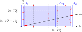
Figure 1: Construction of the candidate sets $\mathfrak{K}_{n_{1}}$ in the two-dimensional setup. Condition (7) is fulfilled if the projection of the left and right edge onto the line spanned by $\phi_{1}$—indicated by the red regions—are disjoint.

Proof

Initially, we consider equispaced Fourier samples along an arbitrary line. For $\zeta\in\bbbr^{D}$ with $\lVert\zeta\rVert=1$, such samples have the form

$$\lvert\hat{\mu}(hm\,\zeta)\rvert^{2}=\lvert\hat{\nu}(hm\,\zeta)\rvert^{2}\,\Bigl{\lvert}\sum_{n=1}^{N}c_{n}\,\mathrm{e}^{-\mathrm{i}hm\langle\zeta,T_{n}\rangle}\Bigr{\rvert}^{2}.$$

Essentially, these samples are the squared Fourier intensities of a point measure on the line with coefficient $c_{n}^{\zeta}\coloneqq c_{n}$ and transitions $T_{n}^{\zeta}\coloneqq\langle\zeta,T_{n}\rangle$. Without loss of generality, we henceforth assume that the families $\mathfrak{C}^{\zeta}\coloneqq[c_{n}^{\zeta}]$ and $\mathfrak{T}^{\zeta}\coloneqq[T_{n}^{\zeta}]$ are ordered such that $0=T_{1}^{\zeta}<\cdots<T_{N}^{\zeta}$. If $\mathfrak{T}^{\zeta}$ is collision-free, and $\mathfrak{C}^{\zeta}$ fulfils $\lvert c_{1}^{\zeta}\rvert\neq\lvert c_{N}^{\zeta}\rvert$, the assumption of Theorem 4.1 are satisfied, and $\mathfrak{C}^{\zeta}$ and $\mathfrak{T}^{\zeta}$ can be determined by Algorithm 2 up to trivial ambiguities. Where the global phase shifts and additional transitions are unproblematic, the conjugated reflection ambiguity has to be resolved. Owing to the distinct absolute values $\lvert\mathfrak{C}\rvert$, we can identify the transitions $T_{n}^{e_{d}}$ with each other. More precisely, for every $n_{1}\in\{1,\dots,N\}$, we find unique indices $n_{2},\dots,n_{D}$ such that $\lvert c_{n_{1}}^{e_{1}}\rvert=\cdots=\lvert c_{n_{D}}^{e_{D}}\rvert$. Up to a global shift, the true transitions $T_{n}$ of (4) are contained in

$$\tilde{\mathfrak{T}}\coloneqq\mathfrak{K}_{1}\cup\cdots\cup\mathfrak{K}_{N}.$$ (6)

with the candidate sets

$$\mathfrak{K}_{n_{1}}\coloneqq\{(T_{n_{1}}^{e_{1}},R_{n_{2}}^{e_{2}},\dots,R_{n_{D}}^{e_{D}}):R_{n_{d}}^{e_{d}}\in\{T^{e_{d}}_{n_{d}},(T^{e_{d}}_{N}-T^{e_{d}}_{n_{d}})\}\}$$

where $\lvert c_{n_{1}}^{e_{1}}\rvert=\cdots=\lvert c_{n_{D}}^{e_{D}}\rvert$. The construction of $\tilde{\mathfrak{T}}$ is schematically illustrated in Fig. 1. Notice that the candidate sets $\mathfrak{K}_{n_{1}}$ are the vertices of $(D-1)$-dimensional cubes lying on shifted versions of the hyperplane orthogonal to $e_{1}$. Therefore, we find $\phi_{d}$ with $\lVert\phi_{d}\rVert=1$ such that $\{e_{1},\phi_{1},\dots,\phi_{D-1}\}$ form a basis and that

$$\langle\phi_{d},S_{1}\rangle\leq\langle\phi_{d},S_{N}\rangle\quad\text{for all}\quad S_{1}\in\mathfrak{K}_{1},S_{N}\in\mathfrak{K}_{N},$$ (7)

see also Fig. 1. Moreover, $\phi_{d}$ may be chosen so that $\mathfrak{T}^{\phi_{d}}$ is collision-free, and Algorithm 2 can be applied to recover $\mathfrak{C}^{\phi_{d}}$ and $\mathfrak{T}^{\phi_{d}}$. Due to (7), the conjugated reflection ambiguity for $\mathfrak{T}^{\phi_{d}}$ can be resolved, and the true transitions are given by

$$\Bigl{\{}\bigl{(}(e_{1}|\phi_{1}|\dots|\phi_{D})^{*}\bigr{)}^{-1}(T_{n_{1}}^{e_{1}},T_{n_{2}}^{\phi_{1}},\dots,T_{n_{D}}^{\phi_{D-1}})^{*}:n_{1}=1,\dots,N\Bigr{\}},$$ (8)

where $*$ denotes the conjugation and transposition, and where the indices are uniquely given by $\lvert c_{n_{1}}^{e_{1}}\rvert=\lvert c_{n_{2}}^{\phi_{1}}\rvert=\cdots=\lvert c_{n_{D}}^{\phi_{D-1}}\rvert$. The reflection of $\mathfrak{T}^{e_{1}}$ would yield the conjugated reflection of $\mu$, which concludes the proof. ∎

Similarly to the recovery guarantee on the line (Theorem 4.1), the proof is constructive and summerizes to the following reconstruction method, which we will also use for the numerical simulations in § 6.

Algorithm 3 (Phase Retrieval on the Real Space)

Input: $D\in\bbbn$, $N\in\bbbn$, $M\geq 2N(N-1)+1$, $h>0$ with $h\lVert T_{n}-T_{k}\rVert<\pi$, adaptive samples of $\lvert\hat{\mu}\rvert^{2}$.

1. Sample $\lvert\hat{\mu}\rvert^{2}$ along the axes to obtain $(\lvert\hat{\mu}(hm\,e_{d})\rvert^{2})_{m=0}^{M}$ for $d=1,\dots,D$.

2. Apply Algorithm 2 to compute $\mathfrak{T}^{e_{d}}$, and build $\tilde{\mathfrak{T}}$ in (6).

3. For $d=1,\dots,D-1$, choose $\theta_{d}\in\bbbr^{D}$ randomly such that (7) is satisfied.

4. Sample $\lvert\hat{\mu}\rvert^{2}$ to obtain $(\lvert\hat{\mu}(hm\,\theta_{d})\rvert^{2})_{m=0}^{M}$.

5. Apply Algorithm 2 to compute $\mathfrak{C}^{\theta_{d}}$ and $\mathfrak{T}^{\theta_{d}}$.

6. Compute $\mathfrak{T}$ by solving the equation system in (8), and set $\mathfrak{C}\coloneqq\mathfrak{C}^{e_{1}}$.

Output: $\mathfrak{C}$, $\mathfrak{T}$.

The statement of Theorem 5.1 remains valid if the unit vectors $e_{d}$ are replaced by an arbitrary basis $\psi_{d}$. Similarly to (8), the candidate set $\tilde{\mathfrak{T}}$ can then be determined by

$$\tilde{\mathfrak{T}}\coloneqq\bigl{(}(\psi_{1}|\dots|\psi_{D})^{*}\bigr{)}^{-1}(\mathfrak{K}_{1}\cup\cdots\mathfrak{K}_{N}).$$ (9)

One of the key assumptions in Theorem 5.1 is that the coordinates of $\mathfrak{T}$ with respect to the considered directions are collision-free. For a given set of transitions $\mathfrak{T}$, this is holds true for almost all directions $\phi\in\bbbr^{D}$, i.e. up to a Lebesgue null set.

Lemma 3

Let $\mathfrak{T}\coloneqq[T_{1},\dots,T_{N}]\subset\bbbr^{D}$ be collision-free, then the family $\mathfrak{T}^{\theta}\coloneqq[\langle\theta,T_{n}\rangle:T_{n}\in\mathfrak{T}]$ is collision-free for almost all $\theta\in\bbbr^{D}$.

Proof

Let $T_{i_{1}}$, $T_{i_{2}}$, $T_{i_{3}}$, $T_{i_{4}}$ be arbitrary points in $\mathfrak{T}$, where only $T_{i_{2}}$ and $T_{i_{3}}$ may coincide. The dimension of the subspace $\{\theta\in\bbbr^{D}:\langle\theta,T_{i_{1}}-T_{i_{2}}\rangle=\langle\theta,T_{i_{3}}-T_{i_{4}}\rangle\}$ may be $D-1$ at the most since $\mathfrak{T}$ is collision-free. Thus the family $\mathfrak{T}^{\theta}$ can only contain collisions for $\theta$ lying in the union of finitely many lower-dimensional subspaces, which gives the assertion. ∎

Against the background of Lemma 3, and since $D$ generic vectors form a basis, the sampling along adaptively chosen lines in the two-dimensional setup can be replaced by the sampling along arbitrary generic lines.

Theorem 5.2 (Phase Retrieval in 2D)

Let $\mu$ be of the form (4) with $\hat{\nu}(\omega)\neq 0$, $\omega\in\bbbr^{2}$, collision-free $\mathfrak{T}$, and distinct $\lvert\mathfrak{C}\rvert$. Further, let $\psi_{1},\psi_{2},\psi_{3}$ be generic vectors in $\bbbr^{2}$. Then $\mu$ can be uniquely reconstructed from

$$\bigl{\{}\lvert\hat{\mu}(hm\,\psi_{d})\rvert:m=0,\dots,2N(N-1)+1,d=1,\dots,3\bigr{\}}$$

up to inevitable ambiguities.

Proof

To establish the statement, we adapt the proof of Theorem 5.1, where $\psi_{1}$, $\psi_{2}$ play the role of $e_{1}$, $e_{2}$, and $\psi_{3}$ the role of the adaptive direction $\phi_{1}$. Due to Lemma 3, the families $\mathfrak{T}^{\phi_{d}}$ are collision-free for generic lines; so the application of Algorithm 2 is unproblematic. Considering the construction of $\mathfrak{K}_{n_{1}}$, we notice that the candidates are contained in a parallelogram, where $\mathfrak{K}_{1}$ and $\mathfrak{K}_{N}$ lie on opposite edges, see Fig. 1 for an illustration. If the coordinates of $\mathfrak{K}_{1}$ and $\mathfrak{K}_{N}$ satisfy (7) with respect to the third direction $\psi_{3}$, we can apply the procedure in the proof of Theorem 5.1 to recover $\mu$. Otherwise, we interchange the role of $\psi_{1}$ and $\psi_{2}$. In this case, we obtain a second set of candidates in the same parallelogram. The new sets $\mathfrak{K}_{1}^{\prime}$ and $\mathfrak{K}_{N}^{\prime}$, however, lie on the remaining to two edges such that $\psi_{3}$ now fulfils (7), and $\mu$ can be recovered. ∎

6 Simulations

To substantiate the theoretical observations, we apply the constructive proof (Algorithm 3) to a minor, synthetic example. Our goal is recover the sparse structure in Fig. 2(a), which consists of five sources. Each source corresponds to a Gaussian with standard derivation $\nicefrac{{1}}{{2}}$ and to a complex coefficient. For repeatability, the exact locations and coefficients are given in Table 1. The Fourier intensity of the true signal is shown in Fig. 2(b). Instead of sampling the whole Fourier domain, we only use equispaced samples on three predefined lines, which are depicted as red lines in Fig. 2(b). The first two lines correspond to the Cartesian axes, and the third to the angle $0.143\pi$. On each line, we take 100 equispaced, noise-free samples, which is slightly more than the 83 samples to employ the univariate, sparse phase retrieval in Algorithm 2. The sampling distance is $h\coloneqq\max\{\lVert T_{k}-T_{n}\rVert\}/2\pi\approx 0.0387$.

(a) Density of $\lvert\mu\rvert$.

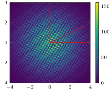
(b) Fourier intensity $\lvert\hat{\mu}\rvert$

Figure 2: Absolute value of the complex-valued density of the true $\mu$ and the corresponding Fourier intensity $\lvert\hat{\mu}\rvert$. The red lines indicate the predefined sampling direction for Algorithm 3.

Table 1: Transitions and coefficients of the true sparse signal $\mu$. Algorithm 3 recovers $\mathfrak{T}$ up to a maximal absolute error of $6.982\cdot 10^{-8}$, and $\mathfrak{C}$ up to a maximal absolute error of $2.898\cdot 10^{-5}$.

$n$	1	2	3	4	5
$T_{n}^{*}$	$(27.374,27.258)$	$(13.065,32.008)$	$(8.847,37.665)$	$(0.000,13.874)$	$(23.876,0.000)$
$c_{n}$	$7.293+5.115\mathrm{i}$	$30.665+2.258\mathrm{i}$	$2.740+22.286\mathrm{i}$	$1.576+49.834\mathrm{i}$	$17.400+46.587\mathrm{i}$

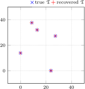
Figure 3: True and recovered transitions $\mathfrak{T}$ and $\mathfrak{T}^{\prime}$ after removing the trivial shift and conjugated reflection ambiguity.

Applying Algorithm 3 here yields an accurate approximation of the true transitions $\mathfrak{T}$. To compare the recovered values $\mathfrak{T}^{\prime}$ with the true ones, we conjugate and reflect the recovered signal such that both signals have the same orientation. Furthermore, we shift both signals so that the leftmost and lowermost vectors lie on the Cartesian axes. The recovered values are shown in Fig. 3 and nearly coincide with the true values. The maximal absolute error after eliminating the shift and conjugated reflection ambiguity is given by

$$\max_{n=1,\dots,5}\{\lvert T_{n}-T^{\prime}_{n}\rvert\}=6.982\cdot 10^{-8}.$$

The maximal absolute error for the coefficients is here

$$\max_{n=1,\dots,5}\{\lvert c_{n}-\mathrm{e}^{\mathrm{i}\alpha}\,c^{\prime}_{n}\rvert\}=2.898\cdot 10^{-5},$$

where we choose the global phase shift $\alpha$ such that the maximal absolute error is minimized.

This first numerical example shows that a sparse, bivariate signal can completely recovered using only samples on three predefined lines instead of sampling the whole Fourier domain. In all fairness, Prony’s method is known to be very sensitive to noise and to become unstable if the frequencies—here $\langle\zeta,T_{n}-T_{k}\rangle$—almost coincide. Since Prony’s method has to recover $2N(N-1)+1$ frequencies for an $N$-sparse signal, $N$ cannot be increased very far. The development of a stable algorithm for the proposed sampling scheme, which can deal with additional noise, thus remains open for further research.

7 Conclusion

The focus of this paper is the sparse phase retrieval problem as it occurs in speckle imaging and crystallography. Combining the one-dimensional phase retrieval approach in [18, 6] with the adaptive sampling strategy from [19], we derive a Prony-based recovery method for $D$-variate, sparse signals. This constructive method is the key ingredient to establish recovery guarantees for collision-free signals. Instead of sampling the Fourier intensity on the entire $D$-dimensional domain, we only require samples from $2D-1$ adaptively chosen or generic lines. This leads to a sampling complexity of $\mathcal{O}(DN^{2})$, where $D$ is the dimension of the signal and $N$ the sparsity level, i.e. the number of shifted components. The $N^{2}$ is accounted for by Prony’s method, which we use to determine the parameters of the given Fourier intensity—an exponential sum with quadratic structure. Since the unknown signal consists of merely $(D+2)N$ real parameters, the question arises whether the signal can also be uniquely recovered using less measurements. This question is left for further research. During the numerical simulations, we show that the Prony-based method can, in principle, be applied to recover the wanted signal from noise-free measurements. Since Prony’s method is, however, very sensitive to noise, one of our next steps is to derive a more stable algorithm for the recovery of specific structured, multivariate signals.

References

- [1] Baechler, G., Kreković, M., Ranieri, J., Chebira, A., Lu, Y.M., Vetterli, M.: Super resolution phase retrieval for sparse signals. IEEE Trans. Signal Process. 67(18), 4839–4854 (2019). https://doi.org/10.1109/TSP.2019.2931169
- [2] Barbotin, Y., Vetterli, M.: Fast and robust parametric estimation of jointly sparse channels. IEEE J. Emerg. Sel. Topics Power Electron. 2(3), 402–412 (2012). https://doi.org/10.1109/JETCAS.2012.2214872
- [3] Beinert, R.: Non-negativity constraints in the one-dimensional discrete-time phase retrieval problem. Inf. Inference 6(2), 213–224 (2017). https://doi.org/10.1093/imaiai/iaw018
- [4] Beinert, R.: One-dimensional phase retrieval with additional interference intensity measurements. Results Math. 72(1-2), 1–24 (2017). https://doi.org/10.1007/s00025-016-0633-9
- [5] Beinert, R., Plonka, G.: Ambiguities in one-dimensional discrete phase retrieval from fourier magnitudes. J. Fourier. Anal. Appl. 21(6), 1169–1198 (2015). https://doi.org/10.1007/s00041-015-9405-2
- [6] Beinert, R., Plonka, G.: Sparse phase retrieval of one-dimensional signals by prony’s method. Front. Appl. Math. Stat. 3, 5 (2017). https://doi.org/10.3389/fams.2017.00005
- [7] Beinert, R., Plonka, G.: Sparse phase retrieval of structured signals by Prony’s method. PAMM 17(1), 829–830 (2017). https://doi.org/https://doi.org/10.1002/pamm.201710382
- [8] Beinert, R., Plonka, G.: Enforcing uniqueness in one-dimensional phase retrieval by additional signal information in time domain. Appl. Comput. Harmon. Anal. 45(3), 505–525 (2018). https://doi.org/10.1016/j.acha.2016.12.002
- [9] Beinert, R., Quellmalz, M.: Total variation-based reconstruction and phase retrieval for diffraction tomography. SIAM J. Imaging Sci. 15(3), 1373–1399 (2022). https://doi.org/10.1137/22M1474382
- [10] Bendory, T., Beinert, R., Eldar, Y.C.: Fourier phase retrieval: uniqueness and algorithms. In: Compressed sensing and its applications, pp. 55–91. Appl. Numer. Harmon. Anal., Birkhäuser, Cham (2017)
- [11] Grohs, P., Koppensteiner, S., Rathmair, M.: Phase retrieval: uniqueness and stability. SIAM Rev. 62(2), 301–350 (2020). https://doi.org/10.1137/19M1256865
- [12] Hildebrand, F.B.: Introduction to Numerical Analysis. Dover Publications, New York, 2nd edn. (1987)
- [13] Klibanov, M.V., Kamburg, V.G.: Uniqueness of a one-dimensional phase retrieval problem. Inverse Problems 30(7), 075004, 10 (2014). https://doi.org/10.1088/0266-5611/30/7/075004
- [14] Klibanov, M.V., Sacks, P.E., Tikhonravov, A.V.: The phase retrieval problem. Inverse Problems 11(1), 1–28 (1995). https://doi.org/10.1088/0266-5611/11/1/001
- [15] Knox, K.T.: Image retrieval from astronomical speckle patterns. J. Opt. Soc. Am. 66(11), 1236–1239 (1976). https://doi.org/10.1364/JOSA.66.001236
- [16] Konijnenberg, A., Coene, W., Pereira, S., Urbach, H.: Combining ptychographical algorithms with the Hybrid Input-Output (HIO) algorithm. Ultramicroscopy 171, 43–54 (2016). https://doi.org/https://doi.org/10.1016/j.ultramic.2016.08.020
- [17] Millane, R.P.: Phase retrieval in crystallography and optics. J. Opt. Soc. Am. A 7(3), 394–411 (1990). https://doi.org/10.1364/JOSAA.7.000394
- [18] Plonka, G., Potts, D., Steidl, G., Tasche, M.: Numerical Fourier analysis. Applied and Numerical Harmonic Analysis, Birkhäuser, Cham (2018). https://doi.org/10.1007/978-3-030-04306-3
- [19] Plonka, G., Wischerhoff, M.: How many Fourier samples are needed for real function reconstruction? J. Appl. Math. Comput. 42(1-2), 117–137 (2013). https://doi.org/10.1007/s12190-012-0624-2
- [20] Potts, D., Tasche, M.: Parameter estimation for exponential sums by approximate prony method. Signal Process. 90(5), 1631–1642 (2010). https://doi.org/10.1016/j.sigpro.2009.11.012
- [21] Prony, R.: Essai expérimental et analytique sur les lois de la dilatabilité des fluides élastiques et sur celles de la force expansive de la vapeur de l’eau et de la vapeur de l’alkool, á différentes températures. Journal de l’École polytechnique 2, 24–76 (1795)
- [22] Ranieri, J., Chebira, A., Lu, Y.M., Vetterli, M.: Phase retrieval for sparse signals: Uniqueness conditions (2013). https://doi.org/10.48550/ARXIV.1308.3058