Adiabatic Quantum Computing for Logistic Transport Optimization

Abstract

Current world trade is based and supported in a strong and healthy supply chain, where logistics play a key role in producing and providing key assets and goods to keep societies and economies going. Current geopolitical and sanitary challenges faced in the entire world have made even more critical the role of logistics and increased demands for tuning transport function to keep the supply chain up and running. The challenge is only increasing and growing for the future, thus tackling transport optimization provides both business and social value. Optimization problems are ubiquitous and they present a challenge due to its complexity, where they´re typically NP-hard problems. Quantum Computing is a developing field, and the Quantum Annealing approach has proven to be quite effective in its applicability and usefulness to tackle optimization problems. In this work we treat the Vehicle Routing Problem, which is also a variation of a famous optimization problem known as the Traveling Salesman Problem. We aim to tackle the vehicle optimization problem from the last mile logistic scenario application, with a perspective from the classical and quantum approaches, and providing a solution which combines both, also known as hybrid solution. Finally, we provide the results of the analysis and proposal for the consideration of applications in a near term business case scenario.

Keywords Quantum Computing  $\cdot$ Quantum Annealing  $\cdot$ Adiabatic  $\cdot$ QUBO  $\cdot$ Optimization  $\cdot$ VRP  $\cdot$ TSP  $\cdot$ Logistics  $\cdot$ Supply Chain  $\cdot$ Last Mile

1 Introduction

The logistic industry, understood as the detailed management and implementation of a business operation, may include the research, sourcing, extraction, manufacturing, production, storing, distributing and transportation of goods and assets. The management of the whole workflow is intensive in data processing and analysis. With the very own specific process depending on the type of goods and assets, there is a key function in the value chain in logistic and supply chain, related to the transportation of assets. Thus, Transport Optimization is an important aspect of logistics improvement. From all the various aspects of the supply chain, we focus our work into the applicability of transport optimization for the “Last Mile” scenario.
Transport Optimization is the process of finding the best way of moving assets from one place (the source location) to another (destination), and is impacted by many distinct factors, like shipment analysis, transport cost structures, rates, and schedules, cargo, routes, delivery requirements and needs, etc. Combining all distinct factors makes this problem an extraordinarily complex combinatorial problem, which demands high computing power to find viable solutions, for this situation resembles and non-polynomial complexity challenge. Also known as NP-hard problem, Transport Optimization, may be rephrased as finding the optimal value for a transport function, and this is where it becomes a high prospect match for current quantum technology approach, through the Quantum Annealing technique.
Throughout this paper, we present the current state of the art in the quantum computing field and dive into the quantum annealing approach to present a viable solution for the Transport Optimization problem. To find the best approach in terms of technology and time-to market applicability, we describe our technique using a hybrid approach, which exploits both classical and quantum techniques to find an optimization model for the Vehicle Routing Problem using Amazon Braket (and the D-Wave quantum annealer). In both cases we provide the results and finally describe our conclusions on the reasons for using a Classical-Quantum approach and recommendations for next steps in a real world use-case scenario.

1.1 Objectives

The main objective of this work is to generate a series of algorithms which can solve cvrp problem instances, the generated algorithms will be compared between each other in order to determine if a quantum or hybrid algorithm is the best option.
A secondary objective is to determine the effects of different hyper-parameters on how the chosen algorithms explore the solution space, the point of this analysis is to determine the best configuration of hyper-parameters in order to better carry out the comparison between classical and quantum algorithms stated in the main objective.
A third objective is to explore possible business use cases for cvrp solvers and the economical impact these solvers could have on the market.

1.2 Outline

This work is organized as follows:

Section 1 provides an overview of the background information necessary to understand this work.
Among this required information one can find descriptions of quantum computing, NP-hardness, the state of the quantum computing field and a description of adiabatic quantum computing, in sections 1.3.1, 1.3.4, 1.3.2 and 1.3.3 respectively.
This section also provides some analysis of the real-world applicability of the problems treated and possible business use cases in subsections 1.4.1 and 1.4.2, it also includes a more in-depth description of the problem this thesis attempts to solve and the constraints applied to said problem in subsections 1.4.3 and 1.4.4 respectively.
Section 2 provides an overview of the strategies used to solve the cvrp problem.
Section 3 details the hybrid approach used to solve the cvrp, subsections 3.1 and 3.2 describe the 2 distinct phases used in the algorithm.
This section also describes the fully quantum algorithm used to solve the cvrp through adiabatic quantum computing in subsection 3.3.
Section 4 provides an experimental analysis of the aforementioned algorithms, as well as details on how to best compose the hybrid algorithm.
The final section 5 describes the conclusions of this work.

1.3 Context

1.3.1 Quantum Computing

A computer is a physical device that helps us process information by executing algorithms, which are well defined instructions, with a well scoped description, to process and analyze information through a well-defined processing task. This processing task is translated into a physical task performed in the computing device.
In a classical computer, these tasks use electromagnetic devices that transfer electronic pulses and perform arithmetical operations using logic gates, to control binary signals, which become the information building blocks, known as bits.

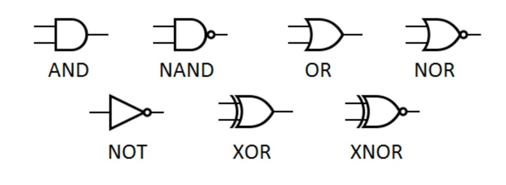
Figure 1: Logic gates [1]

In a quantum computer, these tasks use the quantum mechanical principles to perform operation using unitary gates to control a two-state quantum-mechanical system, known as Qubit. can be represented by a linear superposition of its two orthonormal basis states (or basis vectors). These vectors are usually denoted as $|0\rangle=\begin{bmatrix}1\\ 0\end{bmatrix}$ and $|1\rangle=\begin{bmatrix}0\\ 1\end{bmatrix}$, which is the Dirac conventional notation (or bra-ket notation), where $|0\rangle$ and $|1\rangle$ are known as ket 0 and ket 1 respectively, this is called the computational basis, spanning the two-dimensional linear vector (Hilbert) space.

Figure 2: Quantum Circuit [2]

Since a Qubit can be described as a linear combination of $|0\rangle$ and $|1\rangle$, the quantum state is said to be described by probabilistic amplitudes of the base vectors describing the Hilbert Space. This results in the Qubit having a wider range of probabilities within its vector space. The probabilistic combinations of these amplitudes must sum up to 100%, then the following complies:

$$|\psi\rangle=\alpha|0\rangle+\beta|1\rangle\hskip 14.22636pt\textrm{where}\hskip 14.22636pt|\alpha|²+|\beta|²=1$$ (1)

The possible Quantum States for a single Qubit can be visualized using an artifact called the Bloch Sphere, which provides a graphical description of the Qubit probabilistic description using a geometrical polar description of the qubit coordinates, in the Complex numbers plane

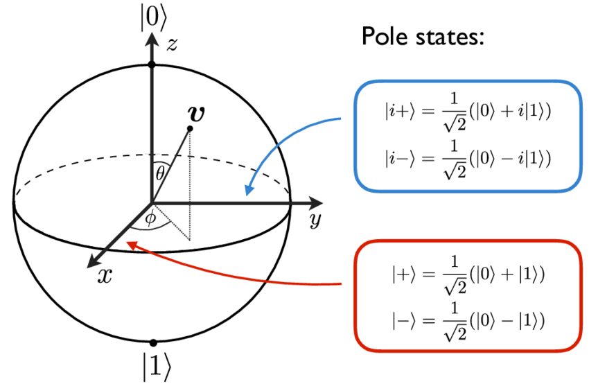
Figure 3: Bloch Sphere [3]

Given this description for the Qubit and its link to a quantum-mechanical system state, it is observable that certain operations can be performed in this quantum state, which then become the building blocks for using quantum mechanics to perform quantum computation through the implementation of quantum circuits using the quantum logic gates approach. These are mathematical operations, becoming unitary operators, described as unitary matrices relative to some basis.
The most common and well know unitary operators are the following:

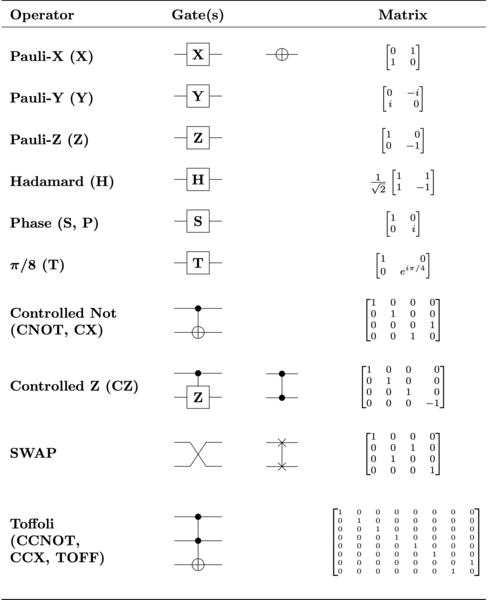
Figure 4: Common quantum logic gates by name, circuit form(s) and matrices [4]

1.3.2 State of the Quantum Computing Field

Quantum Computing is an emerging technology that is based on the Quantum Mechanic effects for achieving increased parallelism in computation power. Developing Quantum Computing started as the most reasonable way to study the quantum properties of nature. In a quick summary of the history of the development of this field, we can summarize the main milestones:

• Mid 1970´s preliminary attempts to create a Quantum Information Theory.

• 1980´s Benioff & Feynman propose the idea that a computer could operate under the laws of Quantum Mechanics.

• In the first half of the 1990´s some important ideas on applicability of quantum computation and initial algorithms arise (Shor´s factorization, Simon´s Oracle later Grove´s algorithm), by the end of the 1990´s the basic ideas of quantum annealing, superconducting circuit and trapped ions transformed into the primary ideas of Quantum Computation applicability, giving rise to the idea of Quantum Computing Industry.

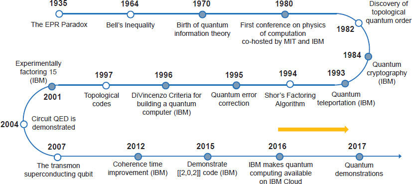
Figure 5: History of quantum computing [5]

Why use quantum computing to tackle complex problems? According to recent research from Boston Consulting Group, 81% of Fortune 500 companies have use cases to develop within the next 3 years, 31% of complex problems are abandoned due to the time and resources required to address them.
Quantum computing is expected to have US$ 850 billion market size by 2040 [6].

1.3.3 Adiabatic Quantum Computing

Adiabatic quantum computation is a form of quantum computing which relies on the adiabatic theorem to do calculations [7], it is very closely related to quantum annealing, although aqc is typically implemented on quantum annealers it has been shown to be polynomially equivalent to circuit model quantum computing [8].
The adiabatic theorem states:

A physical system remains in its instantaneous eigenstate if a given perturbation is acting on it slowly enough and if there is a gap between the eigenvalue and the rest of the Hamiltonian’s spectrum [9].

In other words, a quantum mechanical system will adapt its functional form when exposed to gradually changing external conditions as long as these conditions vary slowly enough, but it will fail to adapt if the conditions vary too quickly.

To solve a problem using aqc we first need to encode the solution to the problem we are trying to solve as the ground state of a Hamiltonian equation, this will be the final Hamiltonian, next we need to prepare a simple Hamiltonian and initialize it to its ground state, this will be the initial Hamiltonian.
To solve the problem we need to slowly evolve the system from the initial Hamiltonian towards the final one, if this evolution is slow enough the system will remain in the ground state, so at the end the state of the system will describe the desired solution.
To apply the Adiabatic Theorem in the Quantum Computing context, the strategy is the following:

1. Design a Hamiltonian whose ground state encodes the solution of an optimization problem.

2. Prepare the known ground state of a simple Hamiltonian.

3. Interpolate slowly.

Hamiltonian Equations:

$$H_{1}=\sum h(x)|x\rangle\langle x|\hskip 14.22636pt\textrm{having}\hskip 14.22636pth(x)=n\sum_{u_{j}u_{k}\in\bar{E}}x_{j}x_{k}-\sum_{u_{j}\in V}x_{j}$$ (2)

$$H_{0}=I-|s\rangle\langle s|\hskip 14.22636pt\textrm{having}\hskip 14.22636pt|s\rangle=\frac{1}{\sqrt{N}}\sum|x\rangle$$ (3)

$$H=(1-t)H_{0}+tH_{1}$$ (4)

1.3.4 NP-Hard Problem Definition

The qubo model has emerged as an underpinning of the quantum computing area known as quantum annealing and its classical counterpart digital annealing [10].
qubo (qubo), also known as unconstrained binary quadratic programming, is a combinatorial optimization problem, originally proposed as a metaheuristic model for solving combinatorial optimization [11], nowadays has a wide range of applications from finance and economics to machine learning. The problem is defined in its most compact way by:

$$f_{Q}(x)=\min x^{t}Qx$$ (5)

This simple model is notable for embracing a remarkable range of applications in combinatorial optimization. For example, the use of this model for representing and solving optimization problems on graphs, facility locations problems, resource allocation problems, clustering problems, set partitioning problems, various forms of assignment problems, sequencing and ordering problems, and many others have been reported in the literature [12].
Let´s review further the problem. A more detailed description of the problem states:
Let the function $f_{Q}:\{0,1\}^{n}\Rightarrow R$ such that:

$$f_{Q}(x)=\sum_{j=1}^{n}\sum_{k=1}^{j}q_{jk}x_{j}x_{k}+\sum_{j=1}^{n}h_{j}x_{j}+c$$ (6)

Find a binary vector $x^{*}$ that is minimal with respect to f among all other binary vectors. This more generalist approach relates closely to the Ising model, which poses a very similar Hamiltonian.
Sometimes, qubo is defined as a maximization instead of a minimization problem, which has no effect on the problem’s complexity class, as maximizing $f_{Q}(x)$ is the same as minimizing $f_{-Q}(x)=-f_{Q}(x)$

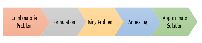
Figure 6: From combinatorial problem towards quantum annealing

1.4 Business Case

1.4.1 Transport Optimization

The Transport Optimization problem, described as the Vehicle Routing Problem is a well-known business scenario where the optimization of logistic processes associated to the loading, programming, clustering and scheduling for vehicles required to follow a path to cover certain destinations under specific constrains, is well measured in terms of business impact.
In the case of the Transport Optimization scenario the range of applicability in logistics is wide and can cover, at the very least, the following possible scenarios:

• Logistics/Material Flow/Assembly Line Optimization

• Grocery Store Logistics

• Sustainable Cities: Waste Collection

• Public Transportation scheduling

• Traffic Routing & Traffic Signal Optimization

• Airline Scheduling/Planning, Routing

• Train Platforming Problem

• Supply Chain Optimization

• Port Scheduling and Planning

The estimated returns on investments in scenarios for transport optimization range from 40% to 60%, since, for instance, Vehicle fleet scheduling is often not optimized effectively, resulting in an unnecessary number of assigned vehicles, lost revenue and waste (e.g., fuel, labor, vehicle wear, etc.), and unnecessary CO2 emissions. This use case is relevant across many industries, including manufacturing, mobility, food delivery, retail, and more.
In a couple of important reference cases, we can consider the piloting and evaluations from Public Transport optimization in Lisbon (Portugal) and New South Wales (Australia). In Lisbon, with car manufacturer Volkswagen; Volkswagen’s traffic management system includes two components: passenger number prediction and route optimization using quantum computing. For the pilot project in Lisbon, 26 stops were selected and connected to form four bus links.
Volkswagen experts have developed a quantum algorithm for route optimization between stops. This algorithm calculates the fastest route for each individual bus in the fleet and optimizes it in near real time. In this way, each bus can bypass bottlenecks along the route at an early stage and avoid traffic jams, even before they arise [13].
In New South Wales, the NSW Government and Transport for NSW have made joint efforts in the application of quantum technologies, for the annual public transportation, passengers take more than 657 million public transport journeys via trains, tubes, buses, ferries and light rail services in NSW and 65 million point-to-point journeys in taxis, car-sharing and rental cars [14].
In a recent study by Boston Consulting Group, the market size for Vehicle Routing Optimization ranges from USD$ 50B to 100B [6], this is also in line with the high potential scenario for optimization in logistics, from the Study from consulting Company McKinsey [15]

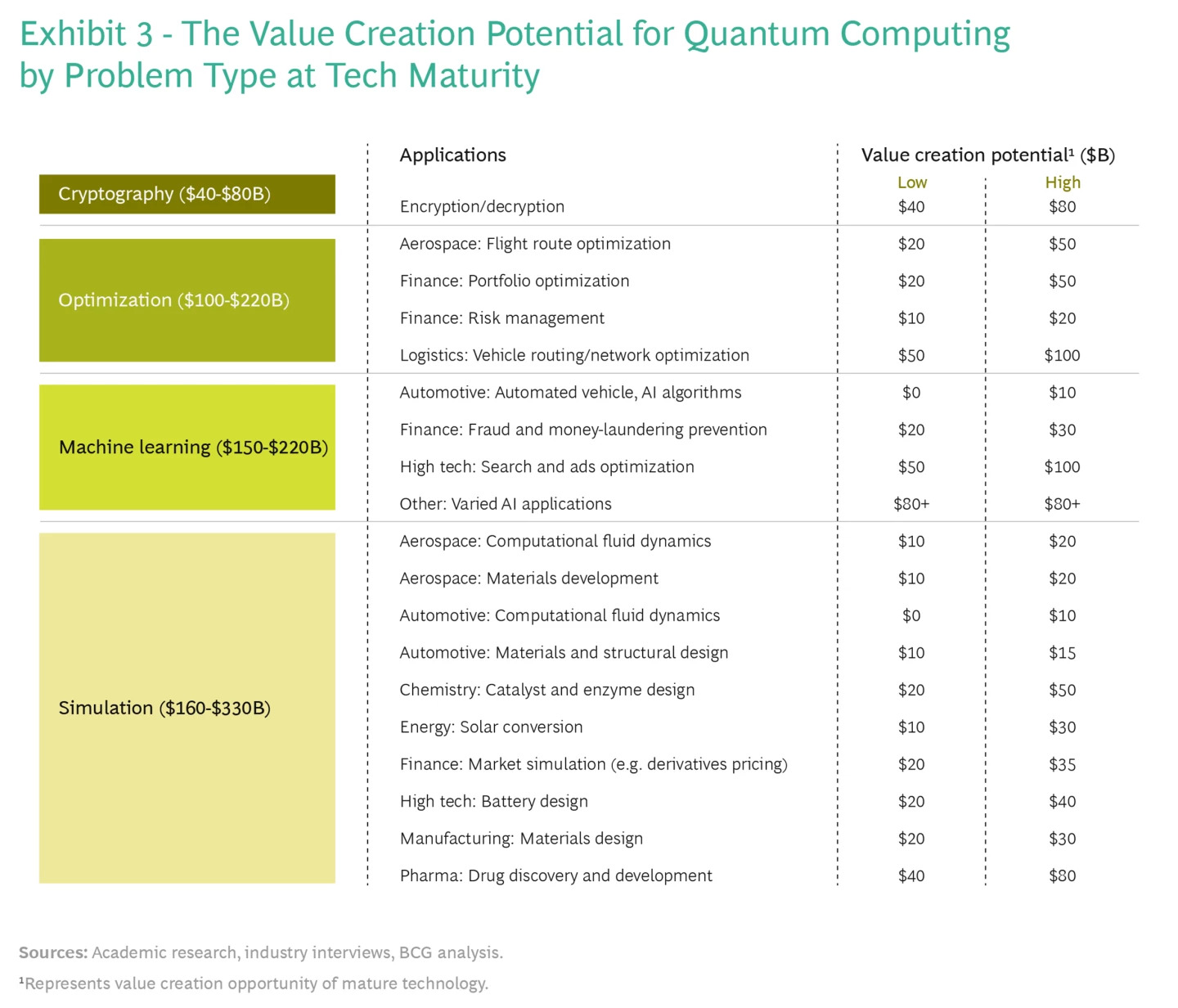
Figure 7: Estimates for the projected value of quantum computing [6]

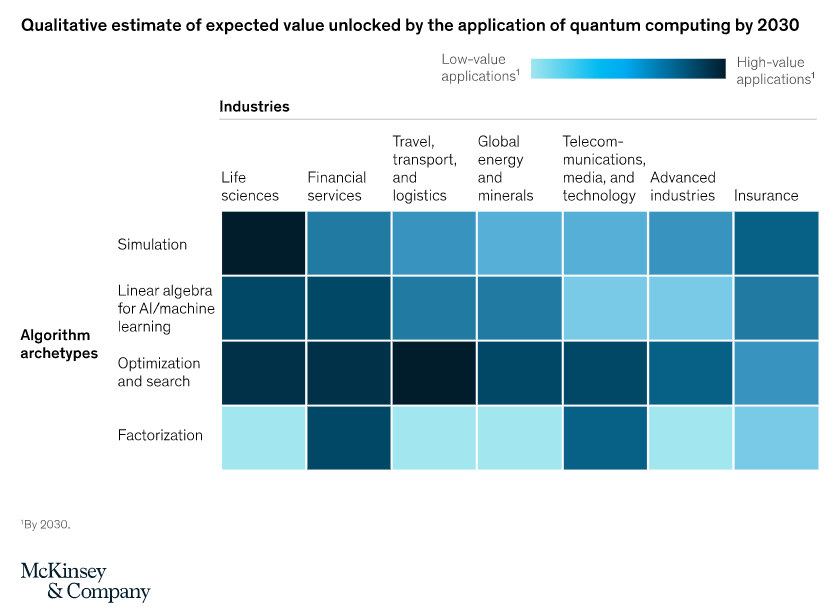
Figure 8: McKinsey estimates Matrix for Value, Industry and Algorithm archetypes [15]

1.4.2 Last Mile Delivery

For our research, we have decided to face the Transport Optimization problem, from the Supply Chain and specifically from the Last Mile delivery challenge, due to its high applicability towards current business challenges.

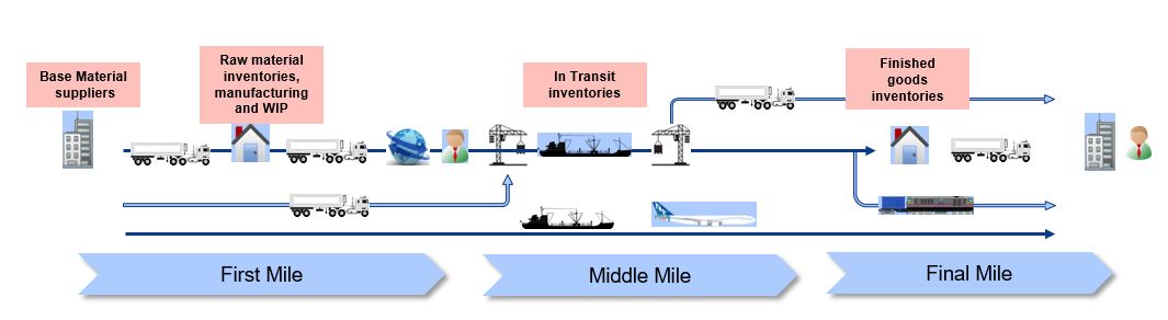
Figure 9: Supply Chain process decoupling [16]

An important part of what is currently known as business state of art is related to understanding the value chain from business and how decoupling business functions may provide agility and scalability to different businesses related to logistics and transportation, looking towards the specialization and optimization of each function, providing and creating value where each business can play the best. Usually, the supply chain can be split into three main stages: the first mile, where the base materials are supplied, arranged, stored, manufactured and/or distributed; the middle mile, where the main transit occurs between the suppliers and the requester, and the last mile, where the finished goods and assets are distributed to its destination to the requester, or customers
The goal of last mile delivery is to transport an item to its recipient in the quickest way possible. This has been driven by the continuously evolving market and demand for convenient customer experience across industries such as e-commerce, food, retail, and many more.
There are many crucial elements involved in the last mile delivery process that customers are looking for, namely the speed, accuracy, time efficiency and precision of the product deliveries after reaching their endpoint.
The boom of e-commerce, propelled by the latest geopolitical and sanitary challenges, has made that, this exponential growth and change in the demands from customers for better solutions, is pushing businesses to seek better solutions as a way of responding to social demands and new economic rules.
The last mile delivery market has been steadily growing in the last decade, and the forecasted opportunity follows the same path. The last mile delivery market in Europe is expected to grow from US$ 677.0 mn in 2018 to US$ 2,491.8 mn by the year 2027 with a cagr of 16.1% from the year 2019 to 2027 [17], while in Spanish speaking Latin America, the level of investment for the last five years is close to US$ 300 mn, leaving Spanish speaking countries like Mexico, Colombia, Chile and Argentina without a leading independent last-mile logistics company, where 60% of the last-mile delivery market is dominated by small, informal companies. This results in inefficiencies due to a lack of technologies such as route optimization as well as a lack of operating scale.
These issues are quickly becoming more pronounced as e-commerce in Latin America has taken off at a compound annual industry growth rate of 16% over the past five years [18]. In the case of Latam, the biggest e-commerce and retailers have made the last mile logistics, the key value differentiator for growth, leveraging the technology tools and analytical processes, to make investments and plannings in advance [19].
The situation in Europe is quite similar for the importance of the optimization in the Last Mile transportation, where key factors driving the region’s market growth include rapid industrialization, the growth of the e-commerce sector, and the presence of large and established logistics players. While Germany is a predominant player in the European market, the main segment responsible for its growth is the b2c sector. In Spain, the Last Mile market is mostly indexed to the b2c sector, which is accountable for over US$ 40 billion e-commerce market size, here the last mile represents around 40% of total costs of logistics operations, in a market dominated up to 80% by small or micro-enterprises [20].
The fact that there are common components in the last mile market makes the proposal from this paper appealing for a close term application of the technology and solution. In a rough estimate, for a market of USD 27 billion in Spain, with an average of 10% margin, where the Last Mile may represent something between 30% to 40% of the total cost, we aim for a 15 billion market, split in a granular small to micro enterprise sector, which is reported to be close to 2000 [21], any 1% savings in optimization can be worth a very competitive Return on Investment.
The fact that there are common components in the last mile market, makes the proposal from this paper appealing for a close term application of the technology and solution. In a rough estimate, for a market of USD 27 billion in Spain, with an average of 10% margin, where the Last Mile may represent something between 30% to 40% of the total cost, we aim for a 15 billion market, split in a granular small to micro enterprise sector, which is reported to be close to 2000 [21], any 1% savings in optimization can prove to be worth a much competitive Return on Investment.
Current investment in the Quantum Computing European Network (in Barcelona) plus the required investment for Human Capital, services and entrepreneurship development, may account for an estimated investment of USD 25 million in 5 years, we summarize the business case as shown in table 1.

Market Size	$ 27,000,000,000
Market Margin	10%
Costs	30%
Num. Operators	2000
Estimated Costs	$ 810,000,000
Est. Unitary Costs	$ 405,000
Gross Inv. Estimate	$ 5,000,000
Estimated Savings	1%
Estimated Savings	$ 8,100,000
roi	62%

Table 1: Preliminary Return on Investments Estimations

1.4.3 VRP Problem

The main problem tackled in this paper is the vrp which is an important combinatorial optimization problem where the main goal is to assign an optimal set of routes to deliver some goods from a given origin (depot) to a given set of destinations (customers), it is a generalization of the well-known vrp in which one vehicle must visit several destinations in an optimal fashion.
Both vrp and tsp are NP-hard problems which makes them exceedingly difficult to solve with classical computing methods since the time taken to solve them grows exponentially with the problem size. Currently the best exact solvers for vrp can solve instances with up to 360 customers [22], this means that they typically cannot be used to solve real world problems where the number of customers can easily range in the thousands, this number gets even worse once you start introducing constraints such as Time-windows, capacity or others which make it more usable in a real-world scenario.
Heuristic solvers can solve instances with many more customers in a reasonable amount of time, though they are usually designed for a specific problem, and they tend to get stuck in local optimum since they explore a limited solution space, meta-heuristic algorithms solve this problem to a certain extent since they work at a higher level of abstraction which allows them to explore more of the solution space [23]. Nonetheless both algorithms are hard to use as general solvers as designing the required Heuristics or Meta-heuristics for the specified constraints is usually a challenging task.
The graph below 10 shows some of the more common constraints applied to the vrp.

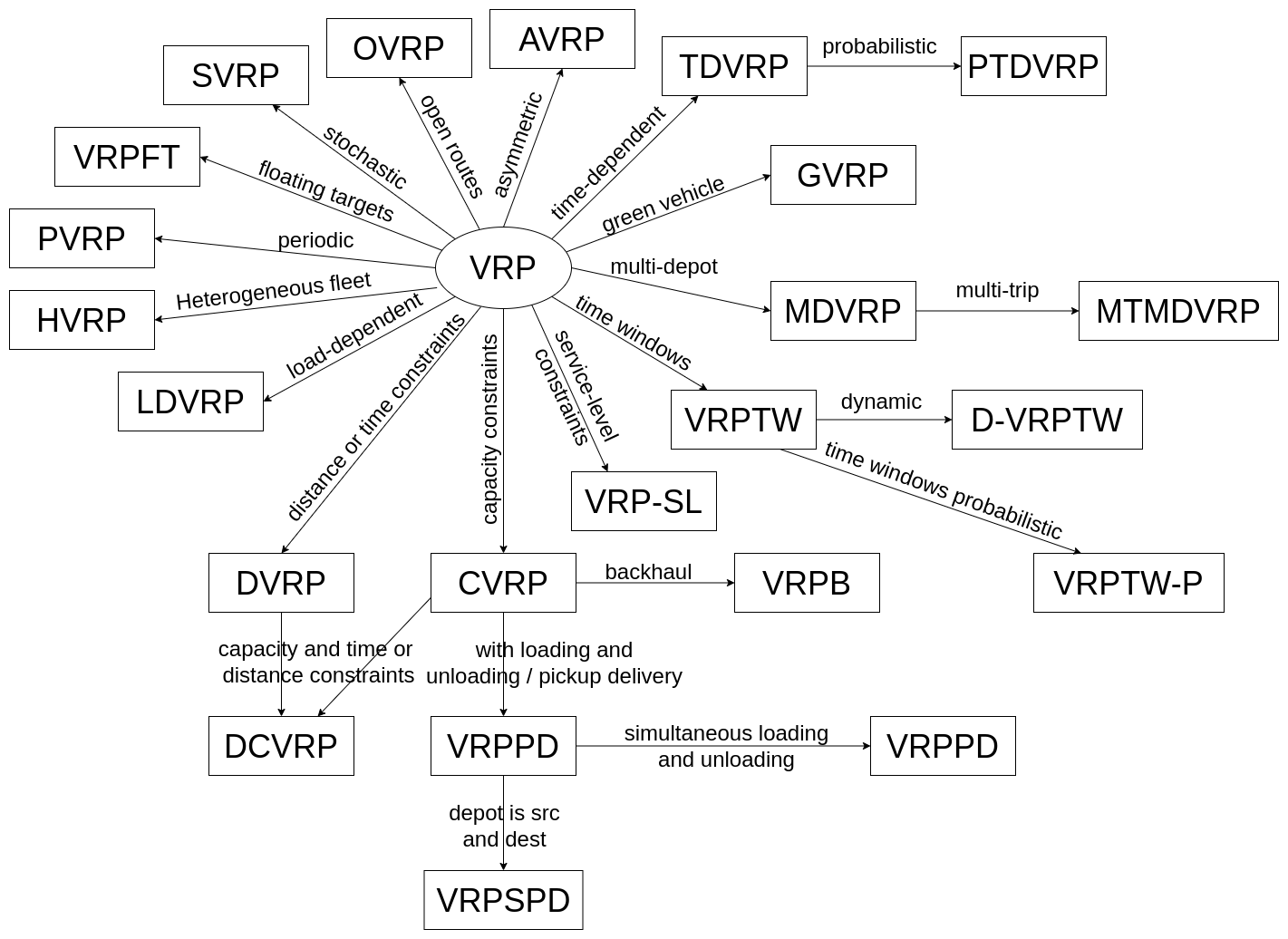
Figure 10: Hierarchy of vrp variants [24]

1.4.4 VRP Constraints

In this paper we tackle the vrp with capacity constraints, also known as cvrp, with single depot, closed routes and homogeneous fleet constraints, this means that we have a single depot, a vehicle fleet with homogeneous capacity and all routes start at the depot and return to it after servicing the customers, the distances between customers are symmetric but the algorithms used can work with asymmetric distances as well by changing the way the distance matrix is calculated. Some of the conditions imposed are that there must be enough vehicles in the depot to cover all customer demand, each customer is serviced by one vehicle and vehicles cannot return to the depot before servicing all the customers in their assigned route.

2 Strategy

2.1 Quantum Annealer

The qpu used for the experiments performed in chapter 4 is D-Wave’s Advantage System 6.1 quantum annealer offered by Amazon Braket, this qpu has 5760 qubits and more than 40,000 couplers; The architecture used by this qpu is called a Pegasus graph, it is a lattice of 16x16 tiles, each tile is made of a basic unit cell which contains 24 qubits, with each qubit coupled to one similarly aligned qubit in the cell and two others in adjacent cells, each cell is composed by a repeated structure where each qubit is coupled to twelve oppositely aligned, and three similarly aligned, qubits. The structure and connectivity of one tile in the Pegasus graph can be described with figure 11, image 12 shows the connectivity structure of a larger Pegasus graph.

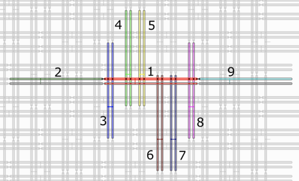
Figure 11: Qubit connectivity inside each tile of the Advantage annealer [25]

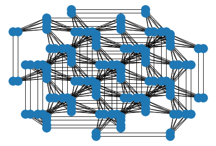
Figure 12: Connectivity structure of a larger Pegasus graph [26]

Due to the topology of the qpu, the qubits have limited connectivity with each other thus to model a qubo problem in the qpu we must first find an embedding of the problem onto the Pegasus graph, this is done with a technique called minor embedding.
This technique maps one graph onto another graph, it is used to map the graph representing the qubo problem onto the Pegasus graph which represents the qpu hardware, this is achieved by sacrificing physical qubits according to the connectivity of the qubo problem.
The minor embedding problem is NP-Hard and for a sufficient number of variables there is no guarantee to find an embedding, with the Advantage qpu this limit is around 145 variables, this greatly limits the amount of problems which can be solved with the qpu, to overcome this limitation D-Wave offers QBSolv.
QBSolv is a hybrid solver that decomposes large qubo problems into smaller sub-problems, these smaller sub-problems are then solved using the tabu algorithm or any configured D-Wave solver such as the Simulated Annealing Solver.
QBSolv will be discontinued by the end of 2022, it is replaced by dwave-hybrid which is a framework designed to create and test workflows that iterate sets of samples through samplers to solve arbitrary-sized qubos, dwave-hybrid includes a reference example sampler called Kerberos, it finds best samples by running in parallel tabu search, simulated annealing and D-Wave subproblem sampling.

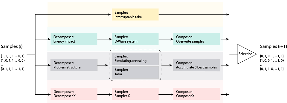
Figure 13: D-Wave hybrid schematic representation with 4 parallel solvers.

2.2 Hybrid Algorithm

The proposed algorithm to solve the cvrp problem with the constraints specified in 1.4.4 is a 2-phase algorithm inspired by [27], this algorithm divides the problem into two separate sub-problems, clustering customers and route optimization, this approach is known as a Cluster-First, Route-Second algorithm, both problems are also NP-Hard but the size of the solution space they need to explore is reduced.

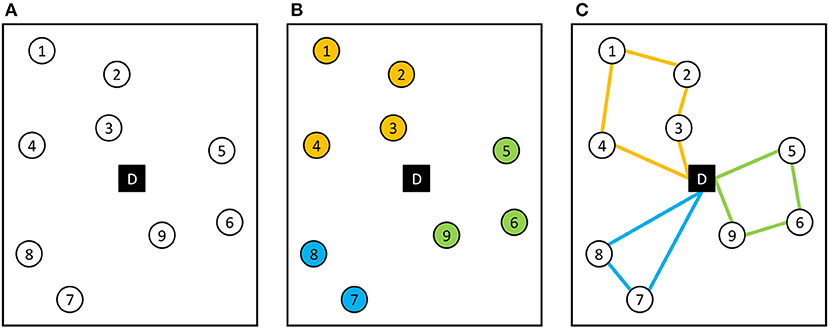
Figure 14: Graphical description of the VRP Problem [27]

For each of the 2 phases we consider both a quantum and a classical approach, the results obtained by these differing approaches are compared to select the best one before composing the final hybrid algorithm.
For the clustering phase the algorithms compared are a modified K-Medoids algorithm for the classical approach and a qubo formulation of the problem for the quantum approach, these will be explained in more detail in sections 3.1.1 and 3.1.2 respectively, the results for the comparison are presented in section 4.1.3.
For the routing phase both presented algorithms attempt to solve the TSP problem, the classical approach is based on combinatorial optimization while the quantum approach models the TSP problem as a qubo formulation, a more detailed explanation of the algorithms is given in sections 3.2.1 for the classical approach and 3.2.2 for the quantum approach, the results of the comparison between both approaches are shown in section 4.2.3.

2.3 QUBO CVRP Solver

We also propose a fully quantum qubo solver, in this solver the cvrp problem is modeled with an equation which minimizes the distance traveled by each vehicle, this equation is subject to 6 additional constraints in the form of qubo equations to more closely model the cvrp constraints explained in section 1.4.4.
The qubo formulation developed for this algorithm is inspired by the formulations presented in [28] and [29], a detailed description of the algorithm and its implementation is given in chapter 3.3.
This algorithm attempts to solve the full cvrp problem at once, it is equivalent to running the clustering phase and the routing phase at the same time, thus it has to deal with a much larger solution space than the hybrid algorithm proposed above.

3 Implementation

3.1 Hybrid Algorithm - Clustering Phase

3.1.1 Classical Clustering

For the classical clustering phase, a K-Medoids algorithm is used to divide the customers into K different clusters, the algorithm is modified to take the total demand of the customers into account such that the distances between customers in the clusters are minimized while the total demand of customers inside each cluster does not surpass the vehicle capacity.
The algorithm is based on the Partitioning Around Medoids algorithm with the added capacity constraint, the steps of the algorithm are the following:

1. Select K data points with the highest demand as the medoids.

2. Determine the clusters by associating each data point to its closest medoid.

3. Compute the initial cluster costs by adding the distances from every point in each cluster to their medoid, add a penalty cost if the total demand of the cluster exceeds the vehicle capacity.

4. While the cluster costs decrease and the maximum number of iterations has not been reached:

   1. For each medoid $m$ and for each non-medoid data point: $n$

      1. Swap $m$ and $o$ and recompute the cluster costs.

      2. If the new cluster cost is higher than the previous one, undo the swap.

   2. Increase number of iterations.

5. Return the clusters.

Algorithm 1 K-Medoids Clustering

Input $M,K,D,Q,I,P$
      Output Clusters Array

1:$\textit{i}\leftarrow 1$

2:$\textit{medoids}\leftarrow K\textit{ data points with the highest demand}$

3:compute_clusters:

4:$\textit{clusters}\leftarrow\textit{associate each data point to its closest medoid}$

5:for each $k\in K$ do

6:     $\textit{clustercosts}_{k}\leftarrow\sum_{n\in clusters_{k}}M_{n,medoids_{k}}$

7:     $\textbf{if }\textit{clustercosts}_{k}>Q\textbf{ then }\textit{clustercosts}_{k}\mathrel{{+}{=}}P$

8:loop:

9:if $\textit{clustercosts}<\textit{prevclustercosts}\And i\leq I$ then

10:     $\textit{prevclusters}\leftarrow\textit{clusters}$

11:     $\textit{prevclustercosts}\leftarrow\textit{clustercosts}$

12:     for each $m\in\textit{medoids}\And n\not\in medoids$ do

13:         $\textit{swap }m\And n$

14:         goto compute_clusters.

15:         if $\textit{clustercosts}>\textit{prevclustercosts}$ then undo the swap               

16:     $i\leftarrow i+1$.

17:     goto loop.

18:     close;

19:return clusters

A pseudocode description of the algorithm is also given in 1, in this description $M$ represents the distance matrix with $M_{ij}$ being the distance from node $i$ to node $j$, $K$ is the number of clusters, $Q$ is the vehicle capacity, $D_{i}$ denotes the demand for customer $i$, $I$ is the maximum number of iterations allowed in the algorithm and $P$ is the penalty cost.
The output is an array of size $|N|$ ($|N|$ is the total number of data points) where the index indicates the customer node and the value which cluster the customer is assigned to.
The penalty cost $P$ is added when the cluster load surpasses the vehicle load capacity, it must be carefully chosen to not override the distance cost inside the clusters, but it must be set high enough so that the distance cost does not override the penalty, or else we might obtain clusters with the correct load but increased customer distance or vice versa, clusters with minimal distance between them but with a load higher than the vehicle capacity.
The running time of the algorithm is slightly reduced by precomputing the distance matrix beforehand which allows us to simply add the distances between each point and the medoid instead of recalculating them at every iteration, other techniques such as memoization and vectorization are also used, but the time complexity of the algorithm is still high, $O(K*(N-K)²)$ where $K$ is the number of clusters and $N$ the total number of data points.
The number of clusters chosen is the number of vehicles available in the depot, this way each vehicle will handle one cluster

Figure 15: Classical clustering on [30] data-set, stars represent the chosen medoids and the number is the total demand inside each cluster

Other clustering algorithms such as K-means could also be used but K-medoids was chosen due to it being less sensitive to outliers than K-means, one of the main disadvantages of both K-medoids and K-means is that the clusters formed are spherical or convex in shape. Density based clustering algorithms such as DBScan do not have this problem and they typically have a lower time complexity ($O(n²)$ for DBScan), but the number of clusters cannot be specified beforehand, recursive DBScan solves this issue by grouping or splitting the clusters as needed until the specified number of clusters is reached, this is the approach used by other algorithms such as DBScan solver [31]

3.1.2 Quantum Clustering

For the quantum clustering phase, we propose a qubo formulation of the clustering algorithm inspired by [32], [33] and [34], with additional constraints applied to assign each customer to a cluster and consider the total demand of customers in each cluster to ensure that it does not exceed the vehicle capacity.
The proposed formulation is shown below (10):

$$M=\sum_{k\in K}\sum_{i,j\in I\\ j>i}dist_{i,j}*x_{i,k}*x_{j,k}$$ (7)

$$C_{1}=\sum_{k\in K}x_{i,k}=1\hskip 14.22636pt\forall i\in I$$ (8)

$$C_{2}=\sum_{i\in I}d_{i}*x_{i,k}\leq C\hskip 14.22636pt\forall k\in K$$ (9)

$$H=M+C_{1}*M_{1}+C2*M_{2}$$ (10)

$K$ is the total number of clusters while $I$ indicates the customer nodes, $dist_{ij}$ represents the distance matrix between all the possible customer nodes, this matrix is precomputed beforehand. $x_{ik}$ is a binary decision variable which indicates if the customer $i$ is assigned to cluster $k$, $C$ represents the available vehicle capacity and $d_{i}$ is the demand of customer $i$.
The qubo formulation is composed of the main objective function $M$ 7 with 2 additional constraints. The formula $M$ tries to find an assignment of customers in clusters such that the total distance between customers in each cluster is minimized, to prevent the formula from not assigning any customer to the clusters, which would obtain a minimum distance of 0, we need to add a penalty for each customer not included in a cluster, this is done through the constraint $C_{1}$ 8.
Constraint $C_{2}$ 9 adds a penalty for each cluster in which the sum of the contained customers demand is greater than the depot vehicle capacity, the formulation is written for a homogeneous vehicle fleet, though extending it to consider a heterogeneous fleet should be trivial, the only change needed is to use a different C value for each cluster.
The multipliers $M_{1}$ and $M_{2}$ are used to assign the weight of the corresponding penalty for each of the 2 constraints; these multipliers must be carefully balanced with the main objective function M to find an adequate solution. If $M_{1}$ is set too high we might obtain a solution where all the customers are assigned to some cluster, but the intra-cluster distance may not be optimal, this typically happens when $C_{1}*M_{1}$ overpowers the objective function, we might also obtain clusters where the sum of the total demand inside it is higher than the vehicle capacity, this happens when $M_{2}$ is set too low. To find an optimal solution the weights of the constraints must be balanced with the objective function, the optimal assignment of these parameters may change on a per problem basis.

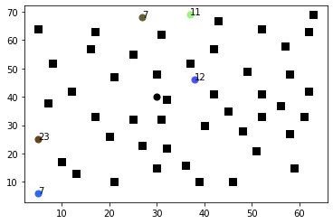
Figure 16: Multiplier effects on the quantum clustering algorithm run on CMT 01 [30] data-set

In the image 16 we can see the effects of the different multipliers, the image on the top left shows the results when the algorithm has $M_{1}$ set too high, the right top image has $M_{1}$ set too low, the left middle image has $M_{2}$ set too high while in the right middle $M_{2}$ is set too low, the left bottom image shows $M_{1}$ and $M_{2}$ well balanced.
The X nodes indicate clusters where the cluster demand exceeds the vehicle capacity, black squares indicate nodes without an assigned cluster, the numbers shown in the graphs represent the total demand of the corresponding cluster.

3.2 Hybrid Algorithm - Routing Phase

3.2.1 Classical Routing

For the classical routing phase, the tsp is modeled as a combinatorial optimization problem which is then solved using OR-Tools. OR-Tools is an open-source software for solving combinatorial optimization problems developed by Google.
The tsp can be modeled inside the OR-Tools framework using the provided rl [35]. This library allows us to model and solve generic routing problems out of the box, while also allowing for some extensibility to customize the models for specific needs, this greatly simplifies the process of designing an algorithm to solve the tsp though it does come with its own set of limitations, namely, there is a limit on the maximum number of nodes that it can handle (32767), a node cannot be visited more than once (except depots which can be starting and ending nodes) and a vehicle cannot transit through a depot.
The rl does have other limitations though these can be considered features more than limitations since they are inherent to the solver instead of constraints on the problem, one is the fact that it uses a node-based model, this approach can solve a wide variety of routing problems though there exist certain problems, such as Arc Routing Problems, which are best solved with a different model; The other feature is the fact that the Routing Library returns approximate solutions, since many routing problems are intractable most of the time a solution close to the global optimum is good enough, otherwise it wouldn’t be able to give any solution at all in a reasonable amount of time.
To define a problem using the rl we indicate the total number of nodes, the number of vehicles and the depot nodes in the Routing Index Manager, the manager is used to define a Routing Model; We also need to define the distance callback function which will return the distance between any 2 nodes, to save on time we precompute the distance matrix beforehand and return the appropriate value in the callback function, this callback function is added to the Routing Model created earlier and will define the cost of each arc traversed by the algorithm. We also need to define a demand callback function which will return the demand associated with a specific node, the demand callback function is then added to the Routing Model as a dimension variable.
With the problem defined in the rl we need to specify the search strategy which will be used to find the solution, the search strategy chosen for our classical algorithm is a meta-heuristic strategy called gls [36], though there are many other search strategies available such as Greedy Search, Tabu Search or Simulated Annealing just to name a few, gls was chosen since it is especially tailored for the rl and has been proven to be particularly successful at solving routing problems [37].

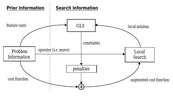
Figure 17: A schematic view of the gls approach to combinatorial optimization problems [38]

gls is built on top of a local search algorithm, it gradually adds penalties to certain features of the solutions to help the local search escape from local minima and plateaus, the gls implementation in the or-tools framework attempts to minimize the following augmented objective function:

$$g(x)=\sum_{(i,j)}d_{ij}(x)+\delta\sum_{(i,j)}(I_{ij}(x)\cdot p_{ij}\cdot c_{ij}(x))$$ (11)

$$I_{ij}=\left\{\begin{array}[]{ c l }1&\quad\textrm{if solution x traverses Arc (i,j)}\\ 0&\quad\textrm{otherwise}\end{array}\right.$$ (12)

Where $d_{ij}=c_{ij}$ denotes the cost of traversing the Arc from $i$ to $j$, $p_{ij}$ is the penalty assigned to feature $I$, $\delta$ is the penalty factor which is used to tune the search to find similar (low $\delta$) or different (high $\delta$) solutions.

3.2.2 Quantum Routing

Simulated annealing is used to solve the tsp inside each cluster in an adiabatic quantum processor, the qubo formulation for the tsp used in the algorithm is based on the qubo formulation for Hamiltonian cycles implemented in [39]. The Hamiltonian cycles problem tries to find a path in a given graph which visits every node (besides the starting node) only once and finally returns to the starting node, the tsp is a trivial extension of the Hamiltonian cycles problem where the weights of each edge in the cycle are minimized.
The qubo formulation for the Hamiltonian cycles problem is given below:

$$C_{1}=\sum_{j\in N+1}(1-\sum_{i\in N+1}x_{i,j})²$$ (13)

$$C_{2}=\sum_{i\in N+1}(1-\sum_{j\in N+1}x_{i,j})²$$ (14)

$$C_{3}=(1-x_{0,0})²$$ (15)

$$H_{A}=C_{1}+C_{2}+C_{3}$$ (16)

$x_{i,j}$ is a binary variable where $i$ represents the order and $j$ represents the customers, $x_{i,j}$ is equal to 1 if the customer with index $j$ is visited in position $i$ in the cycle, $i,j\in{0,…,N}$ where $N$ is equal to the total number of customers.
The first constraint $C_{1}$ 13 ensures that every customer can only appear once in the cycle, the second constraint $C_{2}$ 14 ensures that each position in the cycle must be assigned to only one customer, the third constraint $C_{3}$ 15 is added so that every cycle starts at customer 0, the resulting qubo for the Hamiltonian cycles $H_{A}$ 16 is defined by the sum of all three constraints.
To solve the tsp problem, we need to add a fourth constraint which will minimize the cost of the edges in the cycle 17.

$$H_{B}=\sum_{h\in N+1}\sum_{i\in N+1,h\neq i}\sum_{j\in N}d_{h,i}x_{j,h}x_{j+1,i}$$ (17)

$d$ is the distance matrix which contains the distance between every customer with the depot included as the customer 0, the final qubo is the result of adding $H_{A}$ 16 and $H_{B}$ 17.

$$H=H_{A}*m_{A}+H_{B}*m_{B}$$ (18)

The multipliers $m_{A}$ and $m_{B}$ are used to set the penalties for the distinct parts of the equation, they must be carefully chosen so that one constraint does not override the other, if $m_{A}$ is too high in comparison to $m_{B}$ the result will be a Hamiltonian Cycle but it might not be the one with the shortest path, if the opposite is chosen, $m_{B}$ is too high in comparison to $m_{A}$, the result will be the shortest path but it might not be a Hamiltonian cycle, so there might be some customers left out.

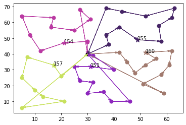
Figure 18: Vehicle routes calculated by the quantum routing algorithm after clustering for the [30] CMT01 data-set

3.3 QUBO CVRP Algorithm

The qubo formulation implemented for this solver is inspired by the formulations presented in [28] and [29], it models the whole cvrp problem as a qubo equation which will be solved with quantum annealing.
To model the cvrp problem with the constraints specified in section 1.4.4 as a qubo equation we first need to define some parameters, we label the number of available vehicles as $K$ and the total number of customers as $C$, $N$ is the total number of customers plus the starting and ending depots ($N=|C|+2$), the starting depot for the routes is always node 0 and the ending depot is always $|C|+1$, the decision variable for our problem is then defined as follows 19:

$$x_{ijk}=\left\{\begin{array}[]{ c l }1&\quad\textrm{if vehicle $k$ travels from node $i$ to node $j$, with ${i,j}\in N$}\\ 0&\quad\textrm{otherwise}\end{array}\right.$$ (19)

Traveling from node $i$ to node $j$ has a cost, this cost is equal to the distance between $i$ and $j$, we label this cost with the variable $c_{ij}$, each customer node also has a certain demand associated with it, we model this demand using the variable $d_{i}$, each vehicle also has a certain capacity, since we are modeling a homogeneous cvrp all vehicles will have the same capacity, this capacity is denoted as $q$.
The main qubo equation used to minimize the total travel cost is the following 20.

$$H=\sum_{k\in K}\sum_{i\in N}\sum_{\begin{subarray}{c}j\in N\\ j\neq i\end{subarray}}c_{ij}\cdot x_{ijk}$$ (20)

This equation is subject to the following constraints:

$$C_{1}=\sum_{k\in K}\sum_{\begin{subarray}{c}j\in N\\ j\neq i\end{subarray}}x_{ijk}=1\hskip 14.22636pt\forall i\in C$$ (21)

$$C_{2}=\sum_{j\in N}x_{0jk}=1\hskip 14.22636pt\forall k\in K$$ (22)

$$C_{3}=\sum_{i\in N}x_{i,|C|+1,k}=1\hskip 14.22636pt\forall k\in K$$ (23)

$$C_{4}=\sum_{\begin{subarray}{c}i\in N\\ i\neq h\end{subarray}}x_{ihk}-\sum_{\begin{subarray}{c}j\in N\\ j\neq h\end{subarray}}x_{hjk}=0\hskip 14.22636pt\forall h\in C,\forall k\in K$$ (24)

$$C_{5}=\sum_{i\in C}\sum_{\begin{subarray}{c}j\in C\\ j\neq i\end{subarray}}d_{i}\cdot x_{ijk}\leq q_{k}\hskip 14.22636pt\forall k\in K$$ (25)

$$C_{6}=\sum_{k\in K}\sum_{i\in S}\sum_{\begin{subarray}{c}j\in S\\ j\neq i\end{subarray}}x_{ijk}\leq|S|-1\hskip 14.22636pt\forall{\begin{subarray}{c}S\in\mathcal{P}(C)\\ 2\leq|S|\leq|C|\end{subarray}}$$ (26)

Constraint $C_{1}$ 21 ensures that each customer is visited only once, constraints $C_{2}$ 22 and $C_{3}$ 23 state that a route must start at depot 0 and end at depot $|C|+1$ respectively, equation $C_{4}$ 24 indicates that after a vehicle arrives at customer $h$ from node $i$ it must leave customer $h$ for node $j$, constraint $C_{5}$ 25 is added to guarantee that the sum of the demand of each customer in the route does not exceed the vehicle capacity $Q$, $q_{k}=Q\forall k\in K$ since we are modeling a homogeneous cvrp.
One of the main problems of formulating the cvrp as a qubo is preventing the formation of impossible routes or closed loops, this happens when a route loops between customers, for example, consider a scenario with one depot, one vehicle and 3 customers, a possible route with closed loops could be $D_{1}\rightarrow C_{1}\rightarrow D_{1}$ and $C_{2}\rightarrow C_{3}$ and $C_{3}\rightarrow C_{2}$ , here the route starts and ends at the depot $D_{1}$ and all customers are visited, however we have a closed loop between customers $C_{2}$ and $C_{3}$. To solve this problem we use the constraint $C_{6}$ 26 which is inspired by the Dantzig–Fulkerson–Johnson formulation of the vrp [40], $\mathcal{P}(C)$ denotes the power set of C.
The constraints presented above need to be reformulated into a qubo formulation, the inequality constraints need to be converted to equality constraints, this is achieved using slack variables, which are auxiliary variables whose final value will not be relevant but help the model consider other solutions. The converted constraints are presented below:

$$C_{1}=\sum_{i\in C}(1-\sum_{k\in K}\sum_{\begin{subarray}{c}j\in N\\ j\neq i\end{subarray}}x_{ijk})²$$ (27)

$$C_{2}=\sum_{k\in K}(1-\sum_{j\in N}x_{0jk})²$$ (28)

$$C_{3}=\sum_{k\in K}(1-\sum_{i\in N}x_{i,|C|+1,k})²$$ (29)

$$C_{4}=\sum_{h\in C}\sum{k\in K}(\sum_{\begin{subarray}{c}i\in N\\ i\neq h\end{subarray}}x_{ihk}-\sum_{\begin{subarray}{c}j\in N\\ j\neq h\end{subarray}}x_{hjk})$$ (30)

$$C_{5}=\sum_{k\in K}((\sum_{i\in C}\sum_{\begin{subarray}{c}j\in C\\ j\neq i\end{subarray}}d_{i}x_{ijk})+\textit{slack}_{Q})$$ (31)

$$C_{6}=\sum_{\begin{subarray}{c}S\in\mathcal{P}(C)\\ 2\leq|S|\leq|C|\end{subarray}}((\sum_{k\in K}\sum_{i\in S}\sum_{\begin{subarray}{c}j\in S\\ j\neq i\end{subarray}}x_{ijk})+\textit{slack}_{S})$$ (32)

To convert the inequalities which appear in constraints $C_{5}$ 25 and $C_{6}$ 26 into minimization problems we need to add slack variables, 33 and 34 respectively, these are auxiliary binary decision variables whose final value is not relevant but which allow the model some flexibility when considering other solutions.

$$\textit{slack}_{Q}=\sum_{i\in{0,...,|Q|}}i\cdot s_{i}\hskip 14.22636pt$$ (33)

$$\textit{slack}_{S}=\sum_{i\in{0,...,|S|}}i\cdot s_{i}\hskip 14.22636pt\forall\begin{subarray}{c}S\in\mathcal{P}(C)\\ 2\leq|S|\leq|C|\end{subarray}$$ (34)

3.4 Requirements

The qubo clustering algorithm, qubo routing algorithm and qubo solver defined in sections 3.1.2, 3.2.2 and 3.3 respectively, are implemented in Python 3.9.7 using the PyQUBO package, the qubo routing algorithm and qubo solver also have different implementations using the Fujitsu Digital Annealer DADK library.
The qubo equations, generated by the algorithms mentioned above, are solved locally using the Simulated Annealing Sampler (neal) and the decomposing solver QBSolv, both provided by D-Wave. They are also solved on a quantum annealer, D-Wave Advantage System 6.1, using Amazon Braket.
The optimization of the qubo equations on real quantum hardware is not as straightforward as with the simulated annealers, depending on the number of variables in the qubo problem it might need to be split into smaller sub-problems in order to "fit" inside the qpu, a more detailed explanation of this is given in section 2.1.
The K-Medoids clustering algorithm and the classical routing algorithm described in sections 3.1.1 and 3.2.1 are also implemented in Python 3.9.7, the K-Medoids algorithm uses the numpy library to perform some of the computations needed and the classical routing algorithm uses the OR-Tools framework provided by Google.
Both classical algorithms (Kmedoids and OR-Routing) as well as the Simulated Annealing Sampler for the qubo problems are run on Pop!_OS 22.04 LTS with a i7-1165G7 Intel CPU and 16 GiB of RAM.
The full code for all the implementations and helper functions can be found at https://github.com/punkyfer/vrpc, the following dependencies are needed to run all the local examples:

• dwave-neal==0.5.9

• dwave-qbsolv==0.3.4

• matplotlib==3.6.0

• numpy==1.23.3

• ortools==9.4.1874

• pandas==1.5.0

• pyqubo==1.2.0

• scikit-learn==1.1.2

• scipy==1.9.1

• xmltodict==0.13.0

• dadk==2022.4.27

4 Results & Analysis

4.1 Hybrid Algorithm - Clustering Phase

4.1.1 Classical Clustering

The K-Medoids clustering algorithm performs a greedy search over the solution space, this means it tends to get "stuck" on local minima, but depending on the structure of the data-set the local minima found is also the global minima.
It performs well on data-sets where the data is structured, this is shown in image 19, or data-sets where the points can be clearly separated into different clusters since in these data-sets there is typically only one minimal solution and thus the greedy search is an adequate method for finding it, we can see this in image 20.

Figure 19: Clusters calculated by the K-Medoids algorithm for the Golden_02 data-set [41]

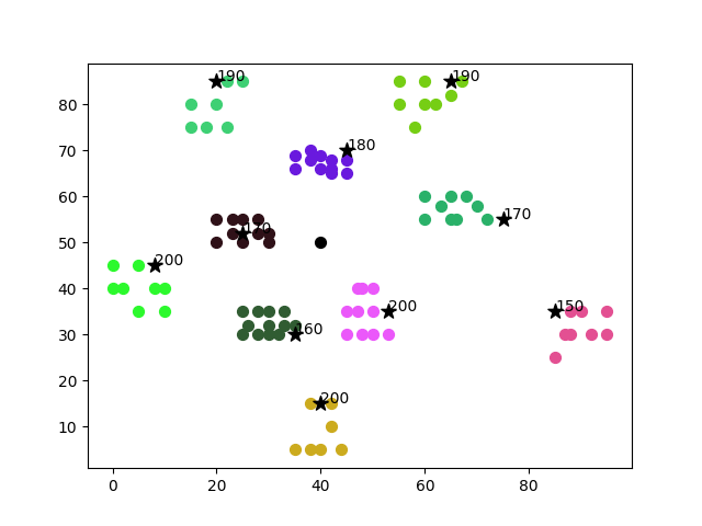
Figure 20: Clusters calculated by the K-Medoids algorithm for the CMT12 data-set

When the points are more randomly distributed the performance of the K-Medoids algorithm suffers and it struggles to find the global minima, this is due to the fact that these data-sets typically have many local minima where the greedy search can get stuck, we can see this in images 21 and 22.

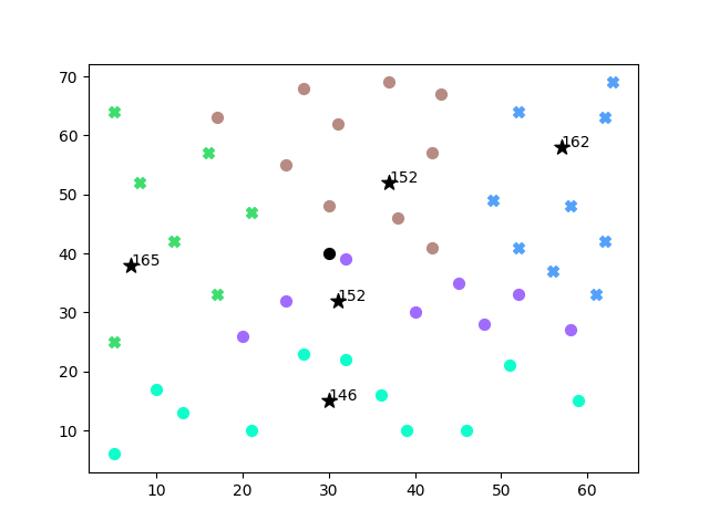
Figure 21: Clusters calculated by the K-Medoids algorithm for the CMT06 data-set

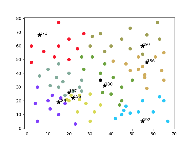
Figure 22: Clusters calculated by the K-Medoids algorithm for the CMT08 data-set

We can observe a relation between the quality of the results obtained by the K-Medoids algorithm and the "clusterability" of the data-set, the better the "clusterability" score of the data, the better the K-Medoids algorithm performs, we can see this in images 20 $\rightarrow$ 23 and 21 $\rightarrow$ 24, the relation between the "clusterability" and the silhouette score obtained by the algorithm is shown in figure 25, though it is not a direct relation since there is some variability on the silhouette score obtained by the K-Medoids algorithm.
The clusterability score of the data is calculated with the method described in An Effective and Efficient Approach for Clusterability Evaluation [42], first we compute the pairwise distances between all the data points, if the data is "clusterable" the distribution of these distance will be multimodal, with one set representing the small intra-cluster distances and the other the longer distances between different cluster, the multi-modality of the data is checked using Hartigan & Hartigan’s dip test for unimodality [43], when the resulting P value is low the probability of the distribution being multi-modal is high, and vice-versa.

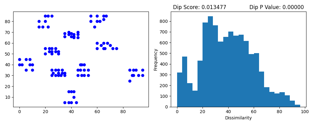
Figure 23: Clusterability score for the CMT12 data-set

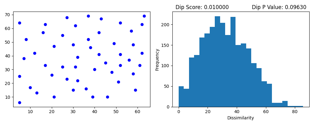
Figure 24: Clusterability score for the CMT06 data-set

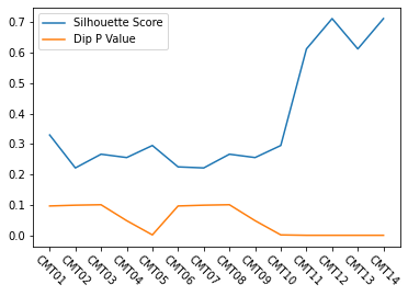
Figure 25: Silhouette score obtained by the K-Medoids algorithm and clusterability score for the CMT 01-14 data-sets

4.1.2 Quantum Clustering

The qubo algorithm used for clustering has 2 multipliers to modify the weights of the different constraints, $M_{1}$ modifies constraint 8 and $M_{2}$ modifies constraint 9, for the experiments we have also added a static multiplier $M_{3}$ to the distance cost shown in equation 7, the resulting equation is shown below 35:

$$M=\sum_{k\in K}\sum_{i,j\in I\\ j>i}M_{3}*dist_{i,j}*x_{i,k}*x_{j,k}$$ (35)

Multiplier $M_{3}$ has a static value of 200, to determine the optimal assignment of the other 2 multipliers ($M_{1}$ and $M_{2}$) we perform a grid search over some possible values and observe the resulting silhouette score of the clusters generated, as well as the number of unassigned nodes and the number of clusters whose demand surpasses the vehicle capacity, these results are plotted as heat maps, images 26 and 27 show the heat maps for the data-sets CMT06 and CMT11 ([30]) respectively.

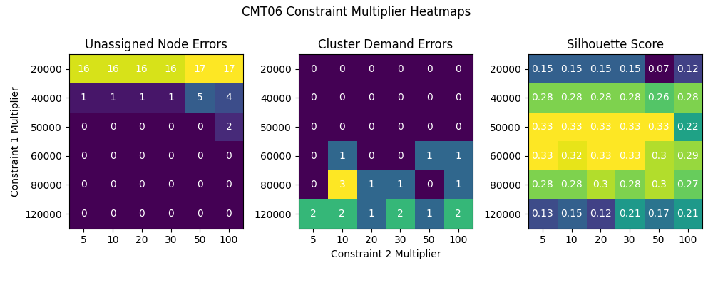
Figure 26: Heat map for the constraint multipliers $M_{1}$ and $M_{2}$ for the CMT06 data-set

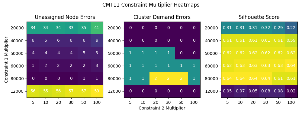
Figure 27: Heat map for the constraint multipliers $M_{1}$ and $M_{2}$ for the CMT11 data-set

We have also plotted a heat map with the averages of all the different normalized results obtained with different data-sets, it is shown in image 28, from this heat map we can observe that the best results obtained by the qubo clustering algorithm occur when the $M_{1}$ multiplier is set to 50,000 and the $M_{2}$ multiplier to 20, though there is some variability between data-sets these parameters offer good results on average.

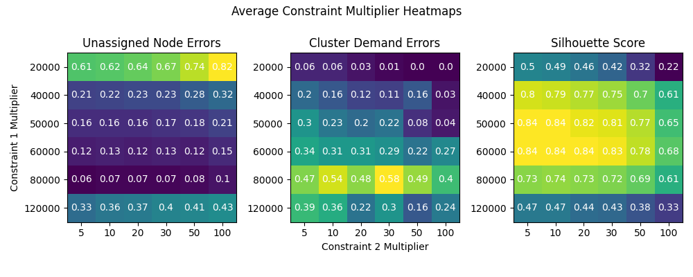
Figure 28: Average heat map for the constraint multipliers $M_{1}$ and $M_{2}$

Another parameter we can modify that also affects the quality of the results obtained by the qubo clustering algorithm is the number of reads/shots specified in the solver, setting a higher number typically allows the algorithm to explore more of the solution space and return a better solution, we can observe this behaviour in image 29, but there comes a point when the algorithm plateaus and increasing the number of reads only increases the computation time without improving the quality of the solution, we can see this happening in image 30 where the solution stops improving after 100 reads.

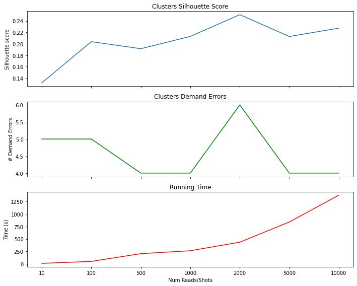
Figure 29: Silhouette score, number of clusters with demand errors and time cost obtained on dataset CMT02 with different number of reads/shots

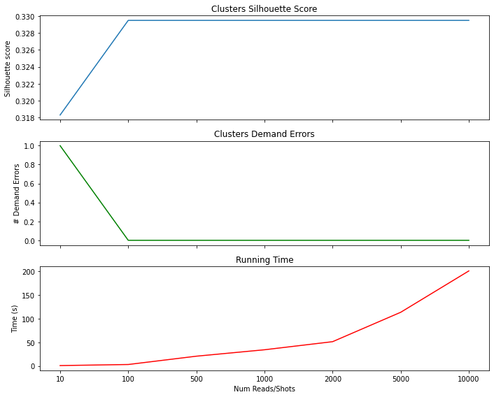
Figure 30: Silhouette score, number of clusters with demand errors and time cost obtained on dataset CMT06 with different number of reads/shots

Choosing an appropriate value for the number of reads is highly dependent on the number of variables in the qubo we are trying to optimize, with higher number of variables requiring a higher number of reads due to the increased size of the solution space, the "clusterability" of the data also plays a role, with more "clusterable" data requiring less reads since the algorithm is able to find the global minima faster.
We ran some experiments with the qubo clustering algorithm on D-Wave’s Advantage System 6.1 provided by Amazon Braket but due to the high number of variables in the qubo and the restrictions on the number of qubits available explained in section 2.1 the cost was prohibitively high, table 2 shows the costs of clustering some CMT data-sets with the qubo clustering algorithm using QBSolv() and 100 shots on Amazon Braket.

Problem	Nodes	Clusters	QUBO Size	Cost ($)
CMT01	50	5	515	9.57
CMT02	75	10	2140	38.28
CMT03	100	8	2392	40*
CMT04	150	12	4188	80*
CMT05	199	16	6368	120*
CMT11	120	7	1540	23.37
* Estimated costs

Table 2: Costs of running the qubo clustering algorithm for some CMT data-sets on D-Wave’s Advantage System 6.1 provided by Amazon Braket

4.1.3 Quantum vs Classical Clustering

From the experiments performed we observe that the 2 clustering functions obtain the same clusters when the data is "clusterable", eg: image 31, with the main difference being the running time of each algorithm, where the K-Medoids algorithm outperforms the qubo equations (0.36s vs 4.61s in the example shown).

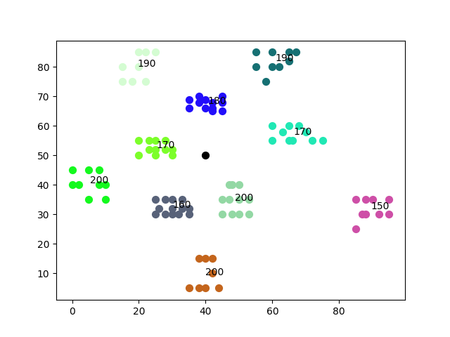
Figure 31: Clusters obtained by K-Medoids algorithm (Left) and qubo algorithm (Right) for the CMT12 data-set

When the data is structured the K-Medoids algorithm performs better than the qubo equations both in quality of the clusters obtained and running time, we can see this in the image 32, the running time of each algorithm for that example is 61.17 seconds for the K-Medoids algorithm and 1922.55 seconds for the qubo equations.

Figure 32: Clusters obtained by K-Medoids algorithm (Left) and qubo algorithm (Right) for the Golden_11 [41] data-set

However when the data is not structured and it has a low "clusterability" score, the qubo algorithm performs better than the K-Medoids algorithm, obtaining a higher silhouette score for the generated clusters and less demand errors in the clusters, this is due to the fact that these solutions typically have many local minima where the K-Medoids algorithm gets stuck while the qubo equations are able to surpass these valleys and reach the global minima, we can see this happening in image 33.

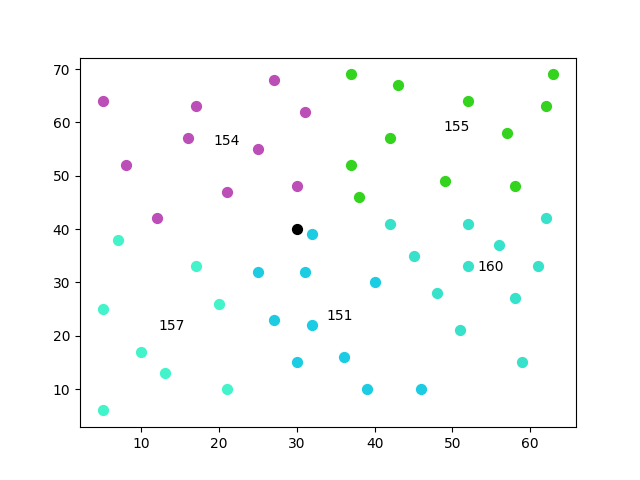
Figure 33: Clusters obtained by K-Medoids algorithm (Left) and qubo algorithm (Right) for the CMT06 data-set

Image 34 shows the silhouette scores and the number of clusters with demand errors obtained by both algorithms on the CMT data-sets, here we can observe that the qubo equations perform slightly better than the K-Medoids algorithm when the data is not clearly "clusterable" (high Dip P value), typically obtaining a higher silhouette score and less number of errors, except in the CMT07 data-set, we can also see that both algorithms obtain the same silhouette score when the data is "clusterable", however the QUBO equations generate clusters with less demand errors than the K-Medoids algorithm.

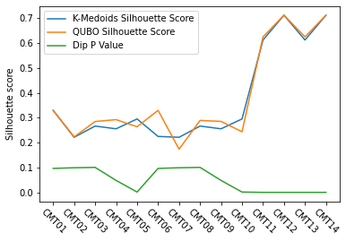
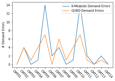
Figure 34: Silhouette score (Left) and demand errors (Right) obtained by K-Medoids algorithm (Left) and QUBO algorithm (Right) for the CMT 01-14 data-sets

The running time of the qubo equations is much higher than the K-Medoids algorithm, though this is expected since the K-Medoids algorithm is designed to run on a classical processor while the qubo equations are designed to be run on a quantum annealer and the experiments are run on the Simulated Annealing Sampler on a classical processor, we can see a comparison of both running times for the CMT data-sets in image 35.

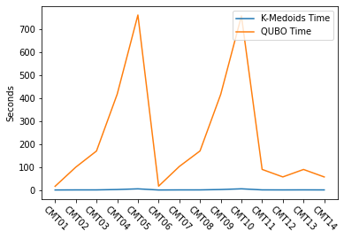
Figure 35: Running time of K-Medoids and qubo algorithms on CMT 01-14 data-sets

4.2 Hybrid Algorithm - Routing Phase

All the experiments for the routing phase are run on the clusters obtained with the K-Medoids algorithm due to the high running time of the qubo clustering algorithm.

4.2.1 Classical Routing

The OR-Tools routing algorithm performs a gls over the solution space, the gls is explained in section 3.2.1, but to recap it is a meta-heuristic method on top of a local search algorithm, gls builds up penalties while exploring the solution space which help the local search algorithm escape the possible local minima and plateaus in said space, this allows the gls algorithm to effectively find the global minima.
Images 36 and 37 show the paths obtained by the OR-Tools routing algorithm when applied to the clusters obtained by the K-Medoids algorithm on the CMT08 and CMT12 data-sets, we can see that the algorithm performs well independently of the distribution of the data points.

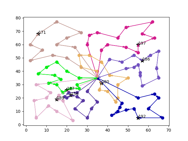
Figure 36: Paths obtained by the OR-Tools routing algorithm for the clusters generated by the K-Medoids algorithm on the CMT08 data-set

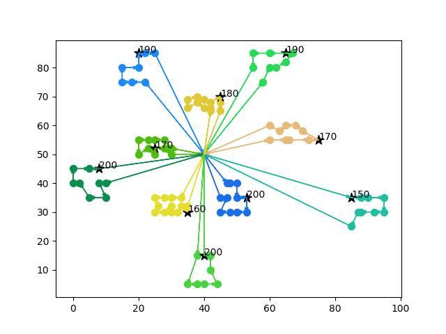
Figure 37: Paths obtained by the OR-Tools routing algorithm for the clusters generated by the K-Medoids algorithm on the CMT12 data-set

We can observe in image 38 that the time taken to find a solution with the OR-Tools routing algorithm increases with the number of vehicles in the data-set, increasing the number of customers/nodes has no effect on the time cost.

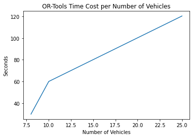
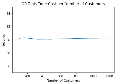
Figure 38: Time cost for the OR-Tools routing algorithm for 100 customers and variable vehicles (Left) and for 10 vehicles and variable customers (Right)

4.2.2 Quantum Routing

The qubo equations used for routing have 2 multipliers to modify the weights of the different constraints, $m_{A}$ modifies constraint 16 and $m_{B}$ modifies constraint 17, to determine the optimal assignment of these multipliers we perform a grid search over some possible values and observe the sum of the distances for the paths generated, as well as the number of errors in these paths, the results are plotted as heat maps, images 39 and 40 show the heat maps for the data-sets CMT06 and CMT12 ([30]) respectively.

Figure 39: Heat map for the constraint multipliers $m_{A}$ and $m_{B}$ for the CMT06 data-set

Figure 40: Heat map for the constraint multipliers $m_{A}$ and $m_{B}$ for the CMT12 data-set

A heat map with the averages of all the normalized results obtained with different data-sets can be seen in image 41, in this heat map we can see that the lowest distance, with the least number of errors, is obtained when the $m_{A}$ multiplier is set to 150 and the $m_{B}$ multiplier to 700, we can slightly reduce the distance further by setting $m_{B}$ to 1,000 but the increase in the number of errors is not worth it.

Figure 41: Average heat map for the constraint multipliers $m_{A}$ and $m_{B}$

The other parameter of the qubo routing algorithm which affects the quality of the results obtained is the number of reads/shots performed by the solver, usually a higher number of reads returns a better solution while increasing the computation time since the algorithm is allowed to explore more of the solution space, we can see this in image 42, but depending on the size of the qubo increasing the number of reads might not offer better solutions while still increasing the computational time, such as in image 43, where the quality of the solution plateaus after 20,000 iterations.

Figure 42: Total distance, qubo solution energy and time cost obtained on dataset CMT12 with different number of reads/shots

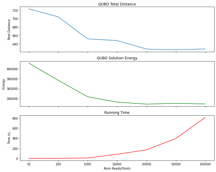
Figure 43: Total distance, qubo solution energy and time cost obtained on dataset CMT06 with different number of reads/shots

The number of reads/shots necessary to find a good solution is highly dependent on the size and complexity of the problem, it must be carefully chosen to not waste computing time, especially when the solver is a real quantum annealer since it has an increased economic cost versus a traditional classic solver.
We ran some experiments with the qubo routing algorithm on D-Wave’s Advantage System 6.1 provided by Amazon Braket but due to the high number of problems generated the cost is high, one advantage of running the qubo routing algorithm after the clustering algorithm is that the problems fit in the quantum annealer without using QBSolv(), table 3 shows the costs of running the qubo routing algorithm on the clusters generated by the K-Medoids algorithm from the CMT data-sets, using 2000 shots on Amazon Braket.

Problem	Nodes	Clusters	Cost ($)
CMT01	50	5	6.8
CMT02	75	10	5.44
CMT03	100	8	8.84
CMT04	150	12	8.84
CMT05	199	16	8.84
CMT11	120	7	12.24

Table 3: Costs of running the qubo routing algorithm for some CMT data-sets on D-Wave’s Advantage System 6.1 provided by Amazon Braket

4.2.3 Quantum vs Classical Routing

From the experiments performed we can observe that the OR-Tools routing algorithm performs better than the qubo equations, obtaining paths with a lower total distance in all the data-sets tested, we can see the total distance of the paths obtained by each algorithm on some of the data-sets in image 44, it is clear that the OR-Tools routing algorithm performs better, though the qubo equations do come close on some data-sets the OR-Tools algorithm still obtains slightly better results.

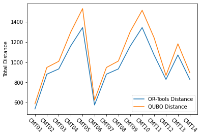
Figure 44: Total distance obtained with OR-Tools and qubo routing algorithms on CMT 01-14 data-sets

Images 45 and 46 show the paths obtained by both routing algorithms for data-sets CMT01 and Golden_05 [41] respectively, we can see that the paths obtained by the OR-Tools routing algorithm are more optimal than the ones obtained by the qubo routing algorithm.

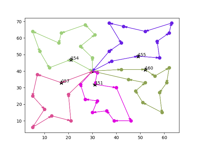
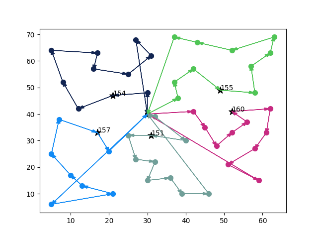
Figure 45: Paths obtained by the OR-Tools routing algorithm (Left) and qubo routing algorithm (Right) on the clusters generated by the K-Medoids algorithm for the CMT01 data-set

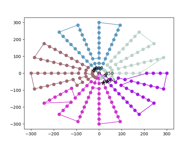
Figure 46: Paths obtained by the OR-Tools routing algorithm (Left) and qubo routing algorithm (Right) on the clusters generated by the K-Medoids algorithm for the Golden_05 data-set

The OR-Tools routing algorithm also performs better than the qubo equations in the time taken to obtain the results, image 47 shows the time cost of each algorithm on some of the data-sets tested, these results are expected since the OR-Tools is designed to run on a classical computer and the qubo equations are designed to run on a quantum annealer, the experiments were performed on a classical computed using the Simulated Annealing Sampler which increases the time cost for the qubo equations.

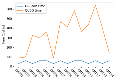
Figure 47: Running time of the OR-Tools and qubo routing algorithms on CMT 01-14 data-sets

4.3 QUBO CVRP Algorithm

The cvrp qubo algorithm explained in chapter 3.3 can only be used in toy problems due to the high number of constraints and variables used in the qubo equation, for the smallest CMT data-set (CMT01) with 50 customers and 5 vehicles the resulting qubo has over 10,000,000 variables, most of these come from the slack variables needed in the closed loop sub-tour elimination constraint 26, with only $\pm$ 14,500 coming from the main equation 20 and the capacity constraint 25, this makes it unfeasible to use on any real data-set.
Even on toy data-sets the performance of the cvrp qubo solver is dismal, it is unable to find a good solution on a data-set with only 6 customers and 2 vehicles, and it generates a qubo with 457 variables, 72 are the main decision variables of the problem, 200 come from the capacity constraint and 129 from the closed loop sub-tour elimination constraint, the results of the experiment are shown below:

  Running...
Same city penalty: 9999999999
Energy of the solution:  232.0
Time elapsed: 370.1921229362488
[[(0, 5), (3, 3), (3, 7), (5, 3)], [(0, 4), (0, 7), (1, 7), (4, 1)],
 [(0, 0), (0, 6), (2, 7), (4, 2), (6, 7)]]
Total distance of all routes: 20000000240.77898

Checking constraints:
   FAIL -> customer 3 is visited 2 times
   FAIL -> Vehicle 2 never arrives at 4 but leaves - (4, 2)
   FAIL -> Vehicle 0 travels between the same cities - (3, 3)
   FAIL -> Vehicle 2 travels between the same cities - (0, 0)
   FAIL -> Vehicle 2 ends at depot 0 - (0, 0)
   FAIL -> Vehicle 2 has capacity 50 and customer load 90
   FAIL -> Vehicle 1 leaves depot 0, 2 times - [(0, 4), (0, 7), (1, 7), (4, 1)]
   FAIL -> Vehicle 2 leaves depot 0, 2 times - [(0, 0), (0, 6), (2, 7), (4, 2), (6, 7)]

Image 48 shows how the number of variables used by the qubo grows as we increase the number of customer nodes and vehicles, we can see that the slack variables used by the capacity constraint increase linearly with the number of vehicles used, the main decision variables and the slack variables used by the closed loop sub-tour elimination both grow exponentially with the number of customers but the main decision variables grow at a much slower rate, the number of main decision variables is also dependent on the number of vehicles while the number of closed loop sub-tour elimination slack variables scales only with the number of customers.

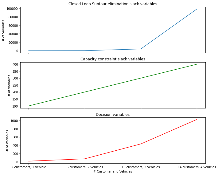
Figure 48: Number of variables generated by the full qubo solver for different number of customers and vehicles

4.4 Findings

From the experiments performed above in section 4.1 we conclude that the best algorithm for the clustering phase of the hybrid algorithm is the qubo clustering algorithm with the multiplier $M_{1}$ set to 50,000 and multiplier $M_{2}$ set to 20, although it offers worse time performance than the K-Medoids algorithm the clusters obtained are usually better, the K-Medoids does perform better when the data points have a clear pattern, but typically real world data does not appear with a clear pattern, thus the qubo clustering algorithm is better suited for real problems.
For the routing phase, we can see in section 4.2 how the OR-Tools routing algorithm outperforms the qubo routing algorithm both in running time and quality of the solution obtained, thus it is the best option for the Hybrid algorithm.
Section 4.3 details the performance of the full qubo solver, although we have not run the same experiment using both the full qubo solver and the hybrid algorithm, it is clear from the experiments run on each of the algorithms independently that the Hybrid algorithm vastly outperforms the full qubo solver.
Table 4 shows a comparison between the best known solutions for the CMT 01-05 data-set and the results obtained by the hybrid algorithm using the qubo clustering algorithm and the OR-Tools routing algorithm, the best known solutions were obtained from Solution of capacitated vehicle routing problem with invasive weed and hybrid algorithms [44].

Problem Instances	BKS*	Hybrid	% Difference with BKS
CMT1(50)	524.61	537.37	2.43
CMT2(75)	835.26	917.95	9.90
CMT3(100)	826.14	933.94	13.05
CMT4(150)	1028.4	1161.26	12.92
CMT5(199)	1291.3	1344.5	4.12
* Best Known Solution

Table 4: Comparison between the best known solutions and the results of the hybrid algorithm for the CMT 01-05 data-sets

5 Conclusions

In this paper we attempted to solve the vrp problem with capacity constraints, single-depot and a homogeneous fleet of vehicles, using both quantum and classical approaches.
The work aimed to understand the potential for a real business use case scenario, focusing on the Last Mile delivery; To this end data-sets with a relatively large number of customers and vehicles were used in the experimentation.

Understanding the current state of development of the related technologies, we proposed a strategy for a hybrid approach, combining and comparing both Classical and Quantum algorithms.
The hybrid algorithm models the vrp problem using a 2-phase approach: clustering/grouping customers and route optimization, this approach is known as a cluster-first, route-second algorithm; For each of the two phases we developed both a quantum and a classical algorithm in order to compare them and determine the most effective combination.
We also developed a fully quantum algorithm to solve the vrp problem by modeling the problem as a QUBO equation subject to multiple constraints.

	Clustering	Routing
Classical	K-Medoids	Combinatorial Optimization
Quantum	QUBO Clustering	QUBO Routing
	QUBO CVRP Algorithm

The evaluation of the quantum algorithms on real quantum hardware has an increased complexity due to the difficulty of embedding the problems on the topology of the available hardware, this is known as the minor embedding problem, currently the biggest quantum annealer offered by Amazon Braket (D-Wave Advantage System 6.1) has a limit of around 145 fully connected variables.
Considering the size of the QUBO equations generated by the developed quantum algorithms and the current condition of the quantum annealers, the additional complexity of the embedding problem decreases the viability of applying the quantum algorithms for the last mile delivery problem at scale.

Classical algorithms typically perform better than their quantum counterparts, though this is not a totally fair comparison since on one hand we have fine-tuned algorithms running on classical computing hardware, and on the other hand we have qubo formulations running on quantum annealers in the nisq era hardware, both technologies are in wildly different edges of the technology maturity ladder.
Despite this disadvantageous situation, we found that under certain circumstances, the quantum clustering algorithm presents an advantage over its classical counterpart, mainly in the scenarios where the "clusterability" rate of the data is lower.
The K-Medoids clustering algorithm performs better when the data can be clearly separated into clusters, however when the data presents a lower rate of "clusterability", or a higher degree of randomness, the quantum clustering approach delivers better results.
We consider this an outstanding finding as it sets the basis for future research into developing quantum algorithms for the constrained clustering problem.
Our findings in the evaluated scenarios lead us to infer that a bigger advantage may be achievable in future versions of quantum hardware, where more qubits and a more interconnected topology may provide better results at larger scales.

The qubo formulation of the cvrp problem given in this paper does not offer good results when compared to the hybrid algorithm due to the increased complexity of the qubo formulation, thus it does not present a realistic alternative.
For the business analysis, we identified the potential for a cost-effective relationship between the cost of running a quantum algorithm and the quality of the results obtained, specially when the data shows a higher degree of randomness, as is usually the case with real customer location data, this demonstrates a theoretical advantage for the quantum computing approach when applied to the constrained clustering problem.

References

- Josh [2021] Josh. Logic gates, 6 2021. URL https://digilent.com/blog/logic-gates/.
- Hui [2018] Jonathan Hui. Qc - programming with quantum gates (single qubits), 12 2018. URL https://jonathan-hui.medium.com/qc-programming-with-quantum-gates-8996b667d256.
- Ketterer [2016] Andreas Ketterer. Modular variables in quantum information. PhD thesis, 10 2016.
- Qua [2019] Quantum logic gate, 2019. URL https://en.wikipedia.org/wiki/Quantum_logic_gate.
- Gumann [2019] Pat Gumann. Domestic Manufacturing Capabilities for Critical DoD Applications. National Academies Press, 11 2019. ISBN 978-0-309-49476-2. doi:10.17226/25499. URL https://www.nap.edu/catalog/25499.
- Bobier et al. [2021] Jean-François Bobier, Matt Langione, Edward Tao, and Antoine Gourévitch. What happens when ‘if’ turns to ‘when’ in quantum computing?, 7 2021. URL https://www.bcg.com/publications/2021/building-quantum-advantage.
- Farhi et al. [2000] Edward Farhi, Jeffrey Goldstone, Sam Gutmann, and Michael Sipser. Quantum computation by adiabatic evolution. 1 2000. doi:10.48550/ARXIV.QUANT-PH/0001106. URL http://arxiv.org/abs/quant-ph/0001106.
- Aharonov et al. [2007] Dorit Aharonov, Wim van Dam, Julia Kempe, Zeph Landau, Seth Lloyd, and Oded Regev. Adiabatic quantum computation is equivalent to standard quantum computation. SIAM Journal on Computing, 37:166–194, 1 2007. ISSN 0097-5397. doi:10.1137/S0097539705447323. URL http://epubs.siam.org/doi/10.1137/S0097539705447323.
- Born and Fock [1928] M. Born and V. Fock. Beweis des adiabatensatzes. Zeitschrift fur Physik, 51:165–180, 3 1928. ISSN 1434-6001. doi:10.1007/BF01343193. URL http://link.springer.com/10.1007/BF01343193.
- Glover et al. [2018] Fred Glover, Gary Kochenberger, and Yu Du. A tutorial on formulating and using qubo models. 11 2018. doi:10.48550/ARXIV.1811.11538. URL http://arxiv.org/abs/1811.11538.
- Kadowaki and Nishimori [1998] Tadashi Kadowaki and Hidetoshi Nishimori. Quantum annealing in the transverse ising model. Physical Review E, 58:5355–5363, 11 1998. ISSN 1063-651X. doi:10.1103/PhysRevE.58.5355. URL https://link.aps.org/doi/10.1103/PhysRevE.58.5355.
- Kochenberger et al. [2014] Gary Kochenberger, Jin-Kao Hao, Fred Glover, Mark Lewis, Zhipeng Lü, Haibo Wang, and Yang Wang. The unconstrained binary quadratic programming problem: a survey. Journal of Combinatorial Optimization, 28:58–81, 7 2014. ISSN 1382-6905. doi:10.1007/s10878-014-9734-0. URL http://link.springer.com/10.1007/s10878-014-9734-0.
- VW_[2019] Volkswagen quantum traffic flow, 2019. URL https://www.volkswagenag.com/en/news/2019/10/volkswagen-optimizes-traffic-flow-with-quantum-computers.html.
- Premier and for Disability Services [2021] Deputy Premier and Minister for Disability Services. A quantum leap in faster and safer travel. Technical report, 2021. URL https://www.nsw.gov.au/media-releases/a-quantum-leap-faster-and-safer-travel.
- Masiowski et al. [2022] Mateusz Masiowski, Niko Mohr, Henning Soller, and Matija Zesko. Quantum computing funding remains strong, but talent gap raises concern. Technical report, 2022. URL https://www.mckinsey.com/business-functions/mckinsey-digital/our-insights/quantum-computing-funding-remains-strong-but-talent-gap-raises-concern.
- Sup [2022] Supply chain whs logistics, 2022. URL https://whs-logistics.com/business.html.
- Partners [2019] The Insight Partners. Europe last mile delivery market to 2027 - regional analysis and forecasts by offerings: Technology (drones, autonomous & semiautonomous vehicles, droids, others); type (b2b, b2c); application (3c products, fresh products, others). Technical report, 2019. URL https://www.businessmarketinsights.com/reports/europe-last-mile-delivery-market.
- Ma [2021] Bob Ma. Last-mile delivery in latin america is ready to take off, 2021. URL https://techcrunch.com/2021/07/22/last-mile-delivery-in-latin-america-is-ready-to-take-off/.
- MundoMarítimo [2020] MundoMarítimo. Mercado libre amplía brecha con falabella y se prepara para enfrentar la irrupción de amazon, 2020. URL MercadoLibreamplíabrechaconFalabellaysepreparaparaenfrentarlairrupcióndeAmazon.
- Segura et al. [2020] Vicente Segura, Ana Fuster, Fernando Antolín, Carlos Casellas, Marta Payno, Alberto Grandío, Albert Cagigós, and Miguel Muelas. Last mile logistics, challenges and solutions in spain. Technical report, 2020. URL https://www2.deloitte.com/content/dam/Deloitte/es/Documents/operaciones/deloitte-es-operations-last-mile.pdf.
- de los Mercados y la Competencia [2021] Comisión Nacional de los Mercados y la Competencia. Informe anual del sector postal (2020). Technical report, 2021. URL www.cnmc.es.
- Pessoa et al. [2019] Artur Pessoa, Ruslan Sadykov, Eduardo Uchoa, and François Vanderbeck. A generic exact solver for vehicle routing and related problems. pages 354–369, 2019. doi:10.1007/978-3-030-17953-3_27. URL http://link.springer.com/10.1007/978-3-030-17953-3_27.
- Ochelska-Mierzejewska et al. [2021] Joanna Ochelska-Mierzejewska, Aneta Poniszewska-Marańda, and Witold Marańda. Selected genetic algorithms for vehicle routing problem solving. Electronics, 10:3147, 12 2021. ISSN 2079-9292. doi:10.3390/electronics10243147. URL https://www.mdpi.com/2079-9292/10/24/3147.
- Režnar et al. [2017] Tomáš Režnar, Jan Martinovič, Kateřina Slaninová, Ekaterina Grakova, and Vít Vondrák. Probabilistic time-dependent vehicle routing problem. Central European Journal of Operations Research, 25:545–560, 9 2017. ISSN 1435-246X. doi:10.1007/s10100-016-0459-2. URL http://link.springer.com/10.1007/s10100-016-0459-2.
- D-Wave [2022] D-Wave. D-wave qpu architecture: Topologies, 2022. URL https://docs.dwavesys.com/docs/latest/c_gs_4.html.
- Amazon-Braket [2022] Amazon-Braket. Anatomy of quantum annealing with d-wave on amazon braket, 2022. URL https://github.com/aws/amazon-braket-examples/blob/main/examples/quantum_annealing/Dwave_Anatomy/Dwave_Anatomy.ipynb.
- Feld et al. [2019] Sebastian Feld, Christoph Roch, Thomas Gabor, Christian Seidel, Florian Neukart, Isabella Galter, Wolfgang Mauerer, and Claudia Linnhoff-Popien. A hybrid solution method for the capacitated vehicle routing problem using a quantum annealer. Frontiers in ICT, 6, 6 2019. ISSN 2297-198X. doi:10.3389/fict.2019.00013. URL https://www.frontiersin.org/article/10.3389/fict.2019.00013/full.
- Harikrishnakumar et al. [2020] Ramkumar Harikrishnakumar, Saideep Nannapaneni, Nam H. Nguyen, James E. Steck, and Elizabeth C. Behrman. A quantum annealing approach for dynamic multi-depot capacitated vehicle routing problem. 5 2020. URL http://arxiv.org/abs/2005.12478.
- Kallehauge et al. [2006] Brian Kallehauge, Jesper Larsen, Oli B.G. Madsen, and Marius M. Solomon. Column Generation. Springer-Verlag, 2006. doi:10.1007/0-387-25486-2_3. URL http://link.springer.com/10.1007/0-387-25486-2_3.
- Christofides et al. [1979] N. Christofides, A. Mingozzi, and P. Toth. Combinatorial Optimization. Wiley, Chichester, 1979.
- Borowski et al. [2020] Michał Borowski, Paweł Gora, Katarzyna Karnas, Mateusz Błajda, Krystian Król, Artur Matyjasek, Damian Burczyk, Miron Szewczyk, and Michał Kutwin. New hybrid quantum annealing algorithms for solving vehicle routing problem. pages 546–561, 2020. doi:10.1007/978-3-030-50433-5_42. URL http://link.springer.com/10.1007/978-3-030-50433-5_42.
- Matsumoto et al. [2022] Nasa Matsumoto, Yohei Hamakawa, Kosuke Tatsumura, and Kazue Kudo. Distance-based clustering using qubo formulations. Scientific Reports, 12:2669, 12 2022. ISSN 2045-2322. doi:10.1038/s41598-022-06559-z. URL https://www.nature.com/articles/s41598-022-06559-z.
- Bauckhage et al. [2019] C Bauckhage, N Piatkowski, R Sifa, D Hecker, and S Wrobel. A qubo formulation of the k-medoids problem. 2019.
- Date et al. [2021] Prasanna Date, Davis Arthur, and Lauren Pusey-Nazzaro. Qubo formulations for training machine learning models. Scientific Reports, 11:10029, 5 2021. ISSN 2045-2322. doi:10.1038/s41598-021-89461-4. URL https://www.nature.com/articles/s41598-021-89461-4.
- Documentation [2015a] Google OR-Tools Documentation. The routing library (rl) in a nutshell, 2015a. URL https://acrogenesis.com/or-tools/documentation/user_manual/manual/tsp/routing_library.html.
- Documentation [2015b] Google OR-Tools Documentation. Guided local search (gls), 2015b. URL https://acrogenesis.com/or-tools/documentation/user_manual/manual/metaheuristics/GLS.html.
- Kilby et al. [1999] Philip Kilby, Patrick Prosser, and Paul Shaw. Meta-Heuristics: Advances and Trends in Local Search Paradigms for Optimization. Springer US, 1999. doi:10.1007/978-1-4615-5775-3_32. URL http://link.springer.com/10.1007/978-1-4615-5775-3_32.
- Voudouris et al. [2010] Christos Voudouris, Edward P.K. Tsang, and Abdullah Alsheddy. Handbook of Metaheuristics. 2010. doi:10.1007/978-1-4419-1665-5_11. URL http://link.springer.com/10.1007/978-1-4419-1665-5_11.
- Lucas [2014] Andrew Lucas. Ising formulations of many np problems. Frontiers in Physics, 2, 2014. ISSN 2296-424X. doi:10.3389/fphy.2014.00005. URL http://journal.frontiersin.org/article/10.3389/fphy.2014.00005/abstract.
- Dantzig et al. [1954] G. Dantzig, R. Fulkerson, and S. Johnson. Solution of a large-scale traveling-salesman problem. Journal of the Operations Research Society of America, 2:393–410, 11 1954. ISSN 0096-3984. doi:10.1287/opre.2.4.393. URL http://pubsonline.informs.org/doi/10.1287/opre.2.4.393.
- Golden et al. [1998] B. L. Golden, E.A. Wasil, J.P. Kelly, and I.-M. Chao. Fleet Management and Logistics. Springer US, 1998. ISBN 978-1-4613-7637-8. doi:10.1007/978-1-4615-5755-5.
- Ackerman et al. [2016] Margareta Ackerman, Andreas Adolfsson, and Naomi Brownstein. An effective and efficient approach for clusterability evaluation. 2 2016.
- Hartigan and Hartigan [1985] J. A. Hartigan and P. M. Hartigan. The dip test of unimodality. The Annals of Statistics, 13, 3 1985. ISSN 0090-5364. doi:10.1214/aos/1176346577.
- Ümit Yıldırım and Kuvvetli [2021] Ümit Yıldırım and Yusuf Kuvvetli. Solution of capacitated vehicle routing problem with invasive weed and hybrid algorithms. International Journal of Industrial Engineering Computations, 12:441–456, 2021. ISSN 19232926. doi:10.5267/j.ijiec.2021.4.002.