Locally uniform random permutations with large increasing subsequences

Abstract

We investigate the maximal size of an increasing subset among points randomly sampled from certain probability densities. Kerov and Vershik’s celebrated result states that the largest increasing subset among $N$ uniformly random points on $[0,1]^{2}$ has size asymptotically $2\sqrt{N}$. More generally, the order $\Theta(\sqrt{N})$ still holds if the sampling density is continuous. In this paper we exhibit two sufficient conditions on the density to obtain a growth rate equivalent to any given power of $N$ greater than $\sqrt{N}$, up to logarithmic factors. Our proofs use methods of slicing the unit square into appropriate grids, and investigating sampled points appearing in each box.

1 Introduction

1.1 Random permutations sampled from a pre-permuton

We start by defining the model of random permutations studied in this paper. Consider points $X_{1},\dots,X_{N}$ in the unit square $[0,1]^{2}$ whose $x$-coordinates and $y$-coordinates are all distinct. One can then naturally define a permutation $\sigma$ of size $N$ the following way: for any $i,j\in[\![1,N]\!]$, let $\sigma(i)=j$ whenever the point with $i$-th lowest $x$-coordinate has $j$-th lowest $y$-coordinate. We denote by $\mathrm{Perm}(X_{1},\dots,X_{N})$ this permutation; see fig. 1 for an example. Now suppose $\mu$ is a probability measure on $[0,1]^{2}$ and that $X_{1},\dots,X_{N}$ are random i.i.d. points distributed under $\mu$: the random permutation $\mathrm{Perm}(X_{1},\dots,X_{N})$ is then denoted by $\mathrm{Sample}_{N}(\mu)$. To ensure this permutation is well defined, we suppose that the marginals of $\mu$ have no atom so that $X_{1},\dots,X_{N}$ have almost surely distinct $x$-coordinates and $y$-coordinates. We call such a measure a pre-permuton; see Section 2.4 for discussion around this name.

Notice that permutations sampled from the uniform measure on $[0,1]^{2}$ are uniformly random. The model of random permutations previously defined thus generalizes the uniform case while allowing for new tools in a geometric framework, as illustrated in [AD95] (see also [Kiw06] for a variant with uniform involutions). This observation motivates the study of such models, as done for example in [AD95] or [Sjö22].

In the present paper we are interested in pre-permutons that are absolutely continuous with respect to Lebesgue measure on $[0,1]^{2}$, and denote by $\mu_{\rho}$ the pre-permuton having density $\rho$. Following [Sjö22] we call sampled permutations under $\mu_{\rho}$ locally uniform. This name is easily understood when $\rho$ is continuous, since the measure $\mu_{\rho}$ can then locally be approximated by a uniform measure.

1.2 Growth speed of the longest increasing subsequence

Figure 1: A family of points and its associated permutation, written in one-line notation $\sigma=\sigma(1)\sigma(2)\dots\sigma(N)$. Here we have $\sigma(1)=2$ because the leftmost point is second from the bottom; and so on.

Let $\sigma$ be a permutation of size $N$. An increasing subsequence of $\sigma$ is a sequence of indices $i_{1}<\dots<i_{k}$ such that $\sigma(i_{1})<\dots<\sigma(i_{k})$. The maximal length of such a sequence is called (length of the) longest increasing subsequence of $\sigma$ and denoted by $\mathrm{LIS}(\sigma)$. Ulam formulated in the 60’s the following question: let us write (here and throughout this paper) for all $N\in\mathbb{N}^{*}$

$$\ell_{N}:=\mathbb{E}\left[\mathrm{LIS}(\sigma_{N})\right]\>\text{where}\>\sigma_{N}\text{ is a uniformly random permutation of size }N,$$

then what can we say about the asymptotic behaviour of $\ell_{N}$ as $N\rightarrow\infty$? The study of longest increasing subsequences has since then been a surprisingly fertile research subject with unexpected links to diverse areas of mathematics [Rom15]. A solution to Ulam’s problem was found by Kerov and Vershik; using objects called Young diagrams through Robinson-Schensted’s correspondance, they obtained the following:

Theorem 1.1 ([VK77]).

$$\ell_{N}\underset{n\rightarrow\infty}{\sim}2\sqrt{N}.$$

The asymptotic behaviour of the longest increasing subsequence in the uniform case is now well understood with concentration inequalities [Fri98, Tal95] and an elegant asymptotic development [BDJ99]. It is then natural to try and generalize Theorem 1.1 to $\mathrm{LIS}\big{(}\mathrm{Sample}_{N}(\mu)\big{)}$ for appropriate pre-permutons $\mu$. One of the first advances on this question was obtained by Deuschel and Zeitouni who proved:

Theorem 1.2 ([DZ95]).

If $\rho$ is a $C_{b}^{1}$, bounded below probability density on $[0,1]^{2}$ then:

$$\frac{1}{\sqrt{N}}\mathrm{LIS}\big{(}\mathrm{Sample}_{N}(\mu_{\rho})\big{)}\underset{N\rightarrow\infty}{\longrightarrow}K_{\rho}$$

in probability, for some positive constant $K_{\rho}$ defined by a variational problem.

This $\sqrt{N}$ behaviour holds more generally when the sampling density is continuous; see 3.3. These results, as well as most of the litterature on the subject, are restricted to the case of a pre-permuton with "regular", bounded density. The goal of this paper is to investigate the asymptotic behaviour of $\mathrm{LIS}\big{(}\mathrm{Sample}_{N}(\mu_{\rho})\big{)}$ when $\rho$ is a probability density on $[0,1]^{2}$ satisfying certain types of divergence. We state in Section 2.2 sufficient conditions on $\rho$ for the quantity $\mathbb{E}\left[\mathrm{LIS}\big{(}\mathrm{Sample}_{N}(\mu_{\rho})\big{)}\right]$ to be equivalent to any given power of $N$ (between $N^{1/2}$ and $N$), up to logarithmic factors. We then present in Section 2.3 a few concentration inequalities for $\mathrm{LIS}\big{(}\mathrm{Sample}_{N}(\mu_{\rho})\big{)}$.

Lastly, it might be worth pointing out that growth rates found in this paper can be seen as "intermediate" in the theory of pre-permutons. Indeed, we previously explained how the $\sqrt{N}$ behaviour corresponds to a "regular" case. In a forthcoming paper we study under which condition the sampled permutation’s longest increasing subsequence behaves linearly in $N$:

Proposition 1.3 ([Dub23]).

Let $\mu$ be a pre-permuton and define

$$\widetilde{\mathrm{LIS}}(\mu):=\max_{A}\mu(A)$$

where the maximum is taken over all increasing subsets of $[0,1]^{2}$, in the sense that any pair of its points is $\prec$-increasing with the notation of Section 2.1. Then the function $\widetilde{\mathrm{LIS}}$ is upper semi-continuous on pre-permutons and satisfies

$$\frac{1}{N}\mathrm{LIS}\big{(}\mathrm{Sample}_{N}(\mu)\big{)}\underset{N\rightarrow\infty}{\longrightarrow}\widetilde{\mathrm{LIS}}(\mu)\quad\text{almost surely}.$$

2 Our results

2.1 Some notation

Throughout the paper, the only order on the plane we consider is the partial order $\prec$ defined by:

$$\text{for all }(x_{1},y_{1}),(x_{2},y_{2})\in\mathbb{R}^{2},\quad(x_{1},y_{1})\prec(x_{2},y_{2})\;\text{ if and only if }\;x_{1}<x_{2}\text{ and }y_{1}<y_{2}.$$

We also write $\mathrm{dist}$ for the $L^{1}$-distance in the plane, namely:

$$\text{for all }(x_{1},y_{1}),(x_{2},y_{2})\in\mathbb{R}^{2},\quad\mathrm{dist}\big{(}(x_{1},y_{1}),(x_{2},y_{2})\big{)}:=|x_{1}-x_{2}|+|y_{1}-y_{2}|,$$

and denote by $\Delta$ the diagonal of the unit square $[0,1]^{2}$. We use the symbol $\mathbb{N}$ for the set of non-negative integers and $\mathbb{N}^{*}$ for the set of positive integers.

Consider points $X_{1},\dots,X_{N}$ in the unit square $[0,1]^{2}$ whose $x$-coordinates and $y$-coordinates are all distinct. Then the quantity $\mathrm{LIS}\big{(}\mathrm{Perm}(X_{1},\dots,X_{N})\big{)}$ is easily read on the visual representation: it is the maximal size of an increasing subset of these points, i.e. the maximal number of points forming an up-right path. For this reason and to simplify notation, we write $\mathrm{LIS}(X_{1},\dots,X_{N})$ for this quantity.

Finally, we use the symbols $\widetilde{O},\widetilde{\Theta},\widetilde{\Omega}$ for asymptotic comparisons up to logarithmic factors: if $(a_{n}),(b_{n})$ be two sequences of positive real numbers, we write $a_{n}=\widetilde{O}(b_{n})$ as $n\rightarrow\infty$ when there exist constants $c_{1}>0$ and $c_{2}\in\mathbb{R}$ such that for some integer $n_{0}$:

$$\text{for all }n\geq n_{0},\quad a_{n}\leq c_{1}\log(n)^{c_{2}}b_{n}.$$

We also write $a_{n}=\widetilde{\Omega}(b_{n})$ when $b_{n}=\widetilde{O}(a_{n})$, and $a_{n}=\widetilde{\Theta}(b_{n})$ when simultaneously $a_{n}=\widetilde{O}(b_{n})$ and $a_{n}=\widetilde{\Omega}(b_{n})$.

2.2 First moment asymptotics of the longest increasing subsequence

Our main results are two conditions on the divergence of the pre-permuton density that imply a large growth rate for the longest increasing subsequences in the sampled permutations. First we study densities diverging at a single point (see the left hand side of fig. 2) and then we study densities diverging along the diagonal (see the right hand side of fig. 2).

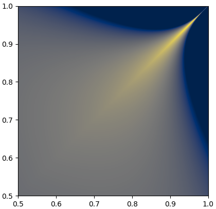
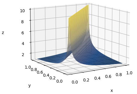
Figure 2: Representation of the divergent densities studied in this paper. On the left, a representation of the density appearing in Theorem 2.2 with $\frac{\beta}{\beta-1}=3$. Bright yellow indicates a high value while dark blue indicates a low value. On the right, the 3D graph of a function satisfying the hypothesis of Theorem 2.4 with $\alpha=-0.5$.

Suppose we have a divergence at the north-east corner, in a radial way around this point. We show in this case that longest increasing subsequences behave similarly to the continuous density case, up to a logarithmic term.

Theorem 2.1.

Suppose the density $\rho$ is continuous on $[0,1]^{2}\setminus\{(1,1)\}$ and satisfies

$$\rho(x,y)=\Theta\left(d^{\alpha}\right)\quad\text{as}\quad(x,y)\rightarrow(1,1)$$

where $d:=\mathrm{dist}((x,y),(1,1))$, for some $\alpha>-2$. Then:

$$\mathbb{E}\left[\mathrm{LIS}\big{(}\mathrm{Sample}_{N}(\mu_{\rho})\big{)}\right]=\underset{N\rightarrow\infty}{\widetilde{\Theta}}\left(\sqrt{N}\right).$$

Note that the condition $\alpha>-2$ is necessary for integrability. In order to see long increasing subsequences appear in the sampled permutations, we will "pinch" the density along the diagonal when approaching the north-east corner. This will force sampled points to concentrate along the diagonal, thus likely forming increasing subsequences, and allow for sharper divergence exponents.

Theorem 2.2.

Suppose the density $\rho$ is continuous on $[0,1]^{2}\setminus\{(1,1)\}$ and satisfies

$$\rho(x,y)=\Theta\left(d^{\frac{\beta}{1-\beta}}\exp\left(-c|x-y|d^{\frac{\beta}{1-\beta}}\right)\right)\quad\text{as}\quad(x,y)\rightarrow(1,1)$$

where $d:=\mathrm{dist}((x,y),(1,1))$, for some $\beta\in]1,2[$ and $c>0$. Then:

$$\mathbb{E}\left[\mathrm{LIS}\big{(}\mathrm{Sample}_{N}(\mu_{\rho})\big{)}\right]=\underset{N\rightarrow\infty}{\widetilde{\Theta}}\left(N^{1/\beta}\right).$$

Note that when $\beta$ varies between $1$ and $2$, the exponent $\frac{\beta}{1-\beta}$ varies between $-\infty$ and $-2$. Note also that such densities exist by integrability of the estimate.

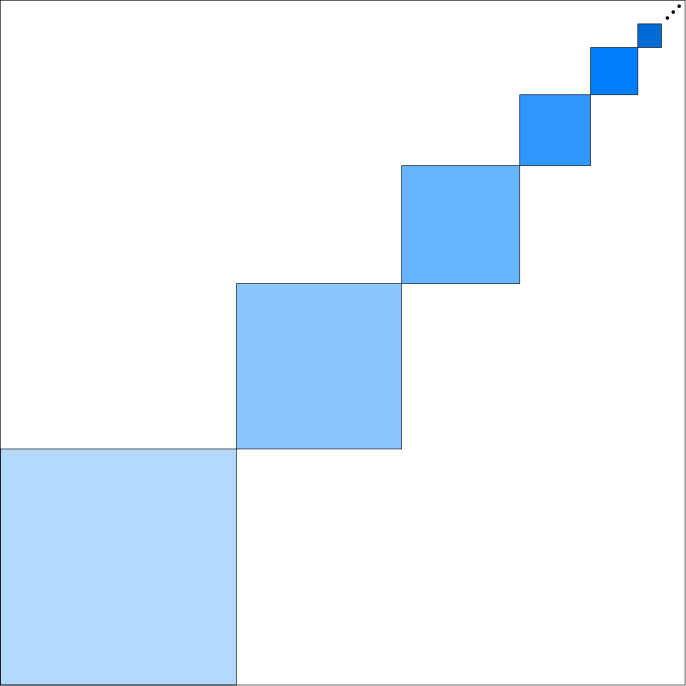
Figure 3: A representation of the permuton $\mu_{\beta,\gamma}^{\nearrow}$. Here, dark blue indicates a high value while light blue indicates a low value of the density.

These previous results rely on a family of "reference" pre-permutons (permutons actually, see Section 2.4) that we now introduce. Fix two parameters $\beta>1$ and $\gamma\in\mathbb{R}$. Define for all positive integer $k\geq 1$

$$u_{k}:=\frac{1}{Z_{\beta,\gamma}}k^{-\beta}\log(k+1)^{\gamma}$$

where

$$Z_{\beta,\gamma}:=\sum_{k\geq 1}k^{-\beta}\log(k+1)^{\gamma},$$

and then for all non-negative integer $n\geq 0$:

$$S_{n}:=\sum_{k=1}^{n}u_{k}\quad\text{and}\quad R_{n}:=\sum_{k>n}u_{k}.$$

Consider the sequence of disjoint boxes

$$\text{for all }n\in\mathbb{N}^{*},\quad C_{n}:=[S_{n-1},S_{n}]^{2},$$

covering the diagonal in an increasing manner. We can then define a probability density on the unit square by

$$\rho_{\beta,\gamma}^{\nearrow}:=\sum_{k\geq 1}u_{k}^{-1}\mathbf{1}_{C_{k}}$$

and we write $\mu_{\beta,\gamma}^{\nearrow}$ for the (pre-)permuton having density $\rho_{\beta,\gamma}^{\nearrow}$ with respect to Lebesgue measure on $[0,1]^{2}$. See fig. 3 for a representation. When $\gamma=0$, we drop the subscript $\gamma$.

Proposition 2.3.

If $\beta\in]1,2[$ and $\gamma\geq 0$ then:

$$\mathbb{E}\left[\mathrm{LIS}\left(\mathrm{Sample}_{N}\left(\mu_{\beta,\gamma}^{\nearrow}\right)\right)\right]=\underset{N\rightarrow\infty}{\widetilde{\Theta}}\left(N^{1/\beta}\right).$$

If $\beta\geq 2$ then:

$$\mathbb{E}\left[\mathrm{LIS}\left(\mathrm{Sample}_{N}\left(\mu_{\beta,\gamma}^{\nearrow}\right)\right)\right]=\underset{N\rightarrow\infty}{\widetilde{\Theta}}\left(\sqrt{N}\right).$$

Lastly we state a result concerning densities diverging along the whole diagonal. This provides a different condition than Theorem 2.2 to obtain a behaviour equivalent to any given power of $N$ (between $N^{1/2}$ and $N$), up to a logarithmic term.

Theorem 2.4.

Suppose the density $\rho$ is continuous on $[0,1]^{2}\setminus\Delta$ and satisfies

$$\rho(x,y)=\Theta\left(|x-y|^{\alpha}\right)\quad\text{as}\quad|x-y|\rightarrow 0$$

for some $\alpha\in]-1,0[$. Then:

$$\mathbb{E}\left[\mathrm{LIS}\big{(}\mathrm{Sample}_{N}(\mu_{\rho})\big{)}\right]=\underset{N\rightarrow\infty}{\widetilde{\Theta}}\left(N^{1/(\alpha+2)}\right).$$

2.3 Concentration around the mean

In this paper we only investigate the mean of $\mathrm{LIS}\big{(}\mathrm{Sample}_{N}(\mu)\big{)}$. The reason is that we can easily deduce asymptotic knowledge of the random variable itself from well known concentration inequalities. In our case it is sufficient to use what’s usually refered to as Azuma’s or McDiarmid’s inequality, found in [McD89] and whose origin goes back to [Azu67]. One of its most common use is for the chromatic number of random graphs, but it is also well adapted to the study of longest increasing subsequences as illustrated in [Fri98].

Theorem 2.5 (McDiarmid’s inequality).

Let $N\in\mathbb{N}^{*}$, $X_{1},\dots,X_{N}$ be independent random variables with values in a common space $\mathcal{X}$ and $f:\mathcal{X}^{N}\rightarrow\mathbb{R}$ be a function satisfying the bounded differences property:

$$\text{for all }i\in[\![1,N]\!]\text{ and }x_{1},\dots,x_{N},y_{i}\in\mathcal{X},\quad|f(x_{1},\dots,x_{i},\dots,x_{N})-f(x_{1},\dots,y_{i},\dots,x_{N})|\leq c$$

for some constant $c>0$. Then for any positive number $\lambda>0$:

$$\mathbf{P}\left(\big{|}f(X_{1},\dots,X_{N})-\mathbb{E}\left[f(X_{1},\dots,X_{N})\right]\big{|}>\lambda\right)\leq 2\exp\left(\frac{-2\lambda^{2}}{Nc^{2}}\right).$$

We can apply this to $\mathrm{LIS}(X_{1},\dots,X_{N})$ where $X_{1},\dots,X_{N}$ are i.i.d. points distributed under $\mu$, noticing that changing the value of a single point changes the size of the largest increasing subset by at most $1$:

Corollary 2.6.

Let $\mu$ be a pre-permuton. Then for any $N\in\mathbb{N}^{*}$ and $\lambda>0$:

$$\mathbf{P}\left(\big{|}\mathrm{LIS}\big{(}\mathrm{Sample}_{N}(\mu)\big{)}-\mathbb{E}\left[\mathrm{LIS}\big{(}\mathrm{Sample}_{N}(\mu)\big{)}\right]\big{|}>\lambda\right)\leq 2\exp\left(\frac{-2\lambda^{2}}{N}\right).$$

This concentration inequality is especially useful when $\mathbb{E}\left[\mathrm{LIS}\big{(}\mathrm{Sample}_{N}(\mu)\big{)}\right]$ is of order greater than $\sqrt{N}$, which is for example the case in Theorem 2.2 when $\beta\in]1,2[$. 2.6 then implies that the variable is concentrated around its mean in the sense that

$$\frac{\mathrm{LIS}\big{(}\mathrm{Sample}_{N}(\mu)\big{)}}{\mathbb{E}\left[\mathrm{LIS}\big{(}\mathrm{Sample}_{N}(\mu)\big{)}\right]}\underset{N\rightarrow\infty}{\longrightarrow}1$$

in probability. Moreover $\mathrm{LIS}\big{(}\mathrm{Sample}_{N}(\mu)\big{)}$ admits a median of order $\widetilde{\Theta}\left(N^{1/\beta}\right)$, and an analogous remark holds for Theorem 2.4. One could then apply the following sharper concentration inequality:

Theorem 2.7 (Talagrand’s inequality for longest increasing subsequences).

Let $\mu$ be a pre-permuton. For any $N\in\mathbb{N}^{*}$, denote by $M_{N}$ a median of $L_{N}:=\mathrm{LIS}\big{(}\mathrm{Sample}_{N}(\mu)\big{)}$. Then for all $\lambda>0$:

$$\mathbf{P}\left(L_{N}\geq M_{N}+\lambda\right)\leq 2\exp\left(\frac{-\lambda^{2}}{4(M_{N}+\lambda)}\right)\quad\text{and}\quad\mathbf{P}\left(L_{N}\leq M_{N}-\lambda\right)\leq 2\exp\left(\frac{-\lambda^{2}}{4M_{N}}\right).$$

See Theorem 7.1.2 in [Tal95] for the original reference in the case of uniform permutations. The proof works the same for random permutations sampled from pre-permutons. See also [Kiw06] for a nice application to longest increasing subsequences in random involutions.

2.4 Discussion

Improvements.

Several hypotheses made in the theorems simplify the calculations but are not crucial to the results. For instance Theorems 2.1 and 2.2 could be generalized by replacing the north-east corner with any point in the unit square and the diagonal with any local increasing curve passing through that point, under appropriate hypotheses. A similar remark holds for Theorem 2.4. We could also state 2.3 for general $\gamma\in\mathbb{R}$, but prefer restricting ourselves to the case $\gamma\geq 0$ since this is all we need for the proofs of Theorems 2.1 and 2.2 and it requires a bit less work.

The necessity of logarithmic terms in our estimates remains an open question. We believe our results could be sharpened in this direction, but our techniques do not seem sufficient to this aim.

Links to permuton and graphon theory.

When $\mu$ is a probability measure on $[0,1]^{2}$ whose marginals are uniform, we call it a permuton [GGKK15]. The theory of permutons was introduced in [HKM⁺13] and is now widely studied [KP13, Muk15, BBF⁺22]. It serves as a scaling limit model for random permutations and is especially useful when investigating models with restriction on the number of occurences of certain patterns [BBF⁺18, BBF⁺20]. One of its fundamental results is that for any permuton $\mu$, the sequence $\big{(}\mathrm{Sample}_{N}(\mu)\big{)}_{N\in\mathbb{N}^{*}}$ almost surely converges in some sense to $\mu$.

Reading this paper does not require any prior knowledge about the litterature on permutons : it is merely part of our motivation for the study of models $\mathrm{Sample}_{N}(\mu)$. Notice however that considering pre-permutons instead of permutons is nothing but a slight generalization. Indeed, one can associate to any pre-permuton $\mu$ a unique permuton $\widetilde{\mu}$ such that random permutations sampled from $\mu$ or $\tilde{\mu}$ have same law [BDMW22].

This paper was partly motivated by [McK19], where an analogous problem is tackled for graphons. The theory of graphons for the study of dense graph sequences is arguably the main inspiration at the origin of permuton theory, and there exist numerous bridges between them [GGKK15, BBD⁺22]. For example the longest increasing subsequence of permutations corresponds to the clique number of graphs. In [DHM15] the authors exhibit a wide family of graphons bounded away from $0$ and $1$ whose sampled graphs have logarithmic clique numbers, thus generalizing this property of Erdős-Rényi random graphs. In some sense this is analogous to Deuschel and Zeitouni’s result on pemutations (Theorem 1.2 here). In [McK19] the author studies graphons allowed to approach the value $1$, and proves in several cases that clique numbers behave as a power of $N$; the results of the present paper are counterparts for permutations.

2.5 Proof method and organization of the paper

The proofs of Theorems 2.1 and 2.2 rely on bounding the density of interest on certain appropriate areas with other densities which are easier to study. This general technique is developped in Section 3 where we prove two lemmas of possible independent interest.

Section 4 is devoted to our reference permutons, which are the main ingredient when bounding general densities. The idea for the proof of 2.3 is that points sampled from $\mu_{\beta,\gamma}^{\nearrow}$ are uniformly sampled on each box $C_{n}$. We can thus use Theorem 1.1 on each box containing enough points, the latter property being studied through appropriate concentration inequalities on binomial variables.

We then prove Theorems 2.1 and 2.2 in Section 5, using all the previously developped tools.

Finally, we prove Theorem 2.4 in Section 6. This proof does not use the previous techniques and rather uses a grid on the unit square that gets thinner as $N\rightarrow\infty$. The main idea is to bound the number of points appearing in any increasing sequence of boxes. The sizes of the boxes are chosen so that a bounded number of points appear in each box, and concentration inequalities are used to make sure such approximations hold simultaneously on every box.

3 Bounds on LIS from bounds on the density

One of the main ideas for the proofs of Theorems 2.1 and 2.2 is to deduce bounds on the order of $\mathrm{LIS}$ from bounds on the sampling density. We state here two useful lemmas to this aim.

Lemma 3.1.

Suppose $f,g$ are two probability densities on $[0,1]^{2}$ such that $f\geq\varepsilon g$ for some $\varepsilon>0$. Then:

$$\mathbb{E}\left[\mathrm{LIS}\big{(}\mathrm{Sample}_{N}(\mu_{f})\big{)}\right]=\underset{N\rightarrow\infty}{\Omega}\left(\mathbb{E}\left[\mathrm{LIS}\big{(}\mathrm{Sample}_{\lfloor\varepsilon N\rfloor}(\mu_{g})\big{)}\right]\right).$$

Likewise, if $f\leq Mg$ for some $M>0$ then

$$\mathbb{E}\left[\mathrm{LIS}\big{(}\mathrm{Sample}_{N}(\mu_{f})\big{)}\right]=\underset{N\rightarrow\infty}{O}\left(\mathbb{E}\left[\mathrm{LIS}\big{(}\mathrm{Sample}_{\lceil MN\rceil}(\mu_{g})\big{)}\right]\right).$$

Proof.

Let us deal with the first assertion of the lemma. We can write

$$f=\varepsilon g+(1-\varepsilon)h$$

for some other probability density $h$ on the unit square. The idea is to use a coupling between those densities. Let $N\in\mathbb{N}^{*}$ and $B_{1},\dots,B_{N}$ be i.i.d. Bernoulli variables of parameter $\varepsilon$, $Y_{1},\dots,Y_{N}$ be i.i.d. random points distributed under density $g$, and $Z_{1},\dots,Z_{N}$ be i.i.d. random points distributed under density $h$, all independent. Then define for all $i$ between $1$ and $N$:

$$X_{i}:=Y_{i}B_{i}+Z_{i}(1-B_{i}).$$

It is clear that $X_{1},\dots,X_{N}$ are distributed as $N$ i.i.d. points under density $f$. Let $I$ be the set of indices $i$ for which $B_{i}=1$. Then

$$\mathrm{LIS}(X_{1},\dots,X_{N})\geq\mathrm{LIS}(Y_{i},i\in I).$$

Hence, if $S_{N}$ denotes an independent binomial variable of parameter $(N,\varepsilon)$:

$$\mathbb{E}\left[\mathrm{LIS}\big{(}\mathrm{Sample}_{N}(\mu_{f})\big{)}\right]\geq\mathbb{E}\left[\mathrm{LIS}\big{(}\mathrm{Sample}_{S_{N}}(\mu_{g})\big{)}\right]\geq\mathbb{E}\left[\mathrm{LIS}\big{(}\mathrm{Sample}_{\lfloor\epsilon N\rfloor}(\mu_{g})\big{)}\right]\mathbf{P}(S_{N}\geq\epsilon N)$$

where that last probability is bounded away from $0$. This concludes the proof of the first assertion. The second one is a simple rewriting of it. ∎

Lemma 3.2.

Suppose $f,g,h$ are probability densities on $[0,1]^{2}$ such that $f\leq c_{1}g+c_{2}h$ for some $c_{1},c_{2}>0$. Then

$$\mathbb{E}\left[\mathrm{LIS}\big{(}\mathrm{Sample}_{N}(\mu_{f})\big{)}\right]=\underset{N\rightarrow\infty}{O}\left(\mathbb{E}\left[\mathrm{LIS}\big{(}\mathrm{Sample}_{\lceil MN\rceil}(\mu_{g})\big{)}\right]+\mathbb{E}\left[\mathrm{LIS}\big{(}\mathrm{Sample}_{\lceil MN\rceil}(\mu_{h})\big{)}\right]\right)$$

for some constant $M>0$.

Proof.

First write $c_{1}g+c_{2}h=M(\lambda g+(1-\lambda)h)$ with appropriate $M>0$ and $\lambda\in]0,1[$. Applying lemma Lemma 3.1 gives us:

$$\mathbb{E}\left[\mathrm{LIS}\big{(}\mathrm{Sample}_{N}(\mu_{f})\big{)}\right]=\underset{N\rightarrow\infty}{O}\left(\mathbb{E}\left[\mathrm{LIS}\left(\mathrm{Sample}_{\lceil MN\rceil}\left(\mu_{\lambda g+(1-\lambda)h}\right)\right)\right]\right).$$

We once again use a coupling argument. Let $N\in\mathbb{N}^{*}$ and $B_{1},\dots,B_{\lceil MN\rceil}$ be i.i.d. Bernoulli variables of parameter $\lambda$, $Y_{1},\dots,Y_{\lceil MN\rceil}$ be i.i.d. random points distributed under density $g$, and $Z_{1},\dots,Z_{\lceil MN\rceil}$ be i.i.d. random points distributed under density $h$, all independent. Then define for all integer $i$ between $1$ and $\lceil MN\rceil$:

$$X_{i}:=Y_{i}B_{i}+Z_{i}(1-B_{i}).$$

It is clear that $X_{1},\dots,X_{\lceil MN\rceil}$ are distributed as $\lceil MN\rceil$ i.i.d. points under density $\lambda g+(1-\lambda)h$. Moreover

$$\mathrm{LIS}(X_{1},\dots,X_{\lceil MN\rceil})\leq\mathrm{LIS}(Y_{1},\dots,Y_{\lceil MN\rceil})+\mathrm{LIS}(Z_{1},\dots,Z_{\lceil MN\rceil})$$

whence

$$\mathbb{E}\left[\mathrm{LIS}\left(\mathrm{Sample}_{\lceil MN\rceil}\left(\mu_{\lambda g+(1-\lambda)h}\right)\right)\right]\leq\mathbb{E}\left[\mathrm{LIS}\big{(}\mathrm{Sample}_{\lceil MN\rceil}\left(\mu_{g}\right)\big{)}\right]+\mathbb{E}\left[\mathrm{LIS}\big{(}\mathrm{Sample}_{\lceil MN\rceil}\left(\mu_{h}\right)\big{)}\right].$$

This concludes the proof. ∎

Before moving on, we state a direct consequence of Lemma 3.1.

Corollary 3.3.

Let $f$ be a continuous probability density on $[0,1]^{2}$. Then:

$$\mathbb{E}\left[\mathrm{LIS}\big{(}\mathrm{Sample}_{N}(\mu_{f})\big{)}\right]=\underset{N\rightarrow\infty}{\Theta}\left(\sqrt{N}\right).$$

Proof.

Since $f$ is continuous on $[0,1]^{2}$, there exists $M>0$ satisfying $f\leq M$. Using Theorem 1.1 and Lemma 3.1 we get:

$$\mathbb{E}\left[\mathrm{LIS}\big{(}\mathrm{Sample}_{N}(\mu_{f})\big{)}\right]=O\left(\ell_{\lceil MN\rceil}\right)=O\left(\sqrt{N}\right)$$

as $N\rightarrow\infty$. Then, $f$ also being non-zero, there exists $\varepsilon>0$ and a square box $C$ contained in $[0,1]^{2}$ such that $f\geq\varepsilon$ on $C$. Since random points uniformly sampled in $C$ yield uniformly random permutations, Theorem 1.1 and Lemma 3.1 imply:

$$\mathbb{E}\left[\mathrm{LIS}\big{(}\mathrm{Sample}_{N}(\mu_{f})\big{)}\right]=\Omega\left(\mathbb{E}\left[\mathrm{LIS}\big{(}\mathrm{Sample}_{\lfloor\varepsilon\mathrm{Leb}(C)N\rfloor}(\mathrm{Leb}_{C})\big{)}\right]\right)=\Omega\left(\ell_{\lfloor\varepsilon\mathrm{Leb}(C)N\rfloor}\right)=\Omega\left(\sqrt{N}\right)$$

as $N\rightarrow\infty$, where $\mathrm{Leb}_{C}$ denotes the uniform probability measure on $C$. We have thus proved the desired estimate. ∎

4 Study of reference permutons

4.1 Preliminaries

The proof of 2.3 hinges on the estimation of binomial variables. We thus state a concentration inequality usually referred to as Bernstein’s inequality. If $\mathcal{S}_{n}$ denotes a binomial variable of parameter $(n,p)$, then:

Lemma 4.1.

$$\text{for all }t>0,\quad\mathbf{P}\left(\left|\mathcal{S}_{n}-np\right|\geq t\right)\leq 2\exp\left(-\frac{-t^{2}/2}{np(1-p)+t/3}\right).$$

See [Ben62, Hoe63] for easy-to-find references and discussion on improvements, and [Ber27] for the original one.

Now let us remind some asymptotics related to the quantities $S_{n}$ and $R_{n}$ introduced in Section 2.2. A short proof is included for completeness.

Lemma 4.2.

For any $\beta>1$ and $\gamma\in\mathbb{R}$ we have

$$\sum_{k\geq n}k^{-\beta}\log(k+1)^{\gamma}\underset{n\rightarrow\infty}{\sim}\frac{n^{1-\beta}}{\beta-1}\log(n)^{\gamma}.$$

Moreover for any $\beta^{\prime}<1$:

$$\sum_{k=1}^{n}k^{-\beta^{\prime}}\log(k+1)^{\gamma}\underset{n\rightarrow\infty}{\sim}\frac{n^{1-\beta^{\prime}}}{1-\beta^{\prime}}\log(n)^{\gamma}.$$

Proof.

First use the integral comparison:

$$\sum_{k\geq n}k^{-\beta}\log(k+1)^{\gamma}\underset{n\rightarrow\infty}{\sim}\int_{n}^{+\infty}x^{-\beta}\log(x+1)^{\gamma}dx$$

and then an elementary integration by parts

$$\int_{n}^{+\infty}x^{-\beta}\log(x+1)^{\gamma}dx =\frac{n^{1-\beta}}{\beta-1}\log(n+1)^{\gamma}-\int_{n}^{+\infty}\frac{x^{1-\beta}}{1-\beta}\gamma\frac{1}{x}\log(x+1)^{\gamma-1}dx$$

$$=\frac{n^{1-\beta}}{\beta-1}\log(n+1)^{\gamma}+\frac{\gamma}{\beta-1}\int_{n}^{+\infty}x^{-\beta}\log(x+1)^{\gamma-1}dx.$$

However, the following holds:

$$\int_{n}^{+\infty}x^{-\beta}\log(x+1)^{\gamma-1}dx=o\left(\int_{n}^{+\infty}x^{-\beta}\log(x+1)^{\gamma}dx\right)\quad\text{as }n\rightarrow\infty.$$

This concludes the proof of the first assertion. The second one is completely similar.

∎

4.2 Proof of Proposition 2.3

In this section we fix $\beta>1$ and $\gamma\geq 0$ and prove 2.3. Consider $N\in\mathbb{N}^{*}$ and write

$$L_{N}:=\mathrm{LIS}\left(\mathrm{Sample}_{N}\left(\mu_{\beta,\gamma}^{\nearrow}\right)\right).$$

Let $X_{1},\dots,X_{N}$ be i.i.d. random variables distributed under $\mu_{\beta,\gamma}^{\nearrow}$. For each $k\in\mathbb{N}^{*}$, define

$$\mathcal{X}_{N,k}:=\{X_{1},\dots,X_{N}\}\cap C_{k}$$

and let $N_{k}$ be the cardinal of $\mathcal{X}_{N,k}$, i.e. the number of points appearing in box $C_{k}$. Each $N_{k}$ is a binomial variable of parameter $(N,u_{k})$, and

$$\sum_{k\geq 1}N_{k}=N.$$

Conditionally on $N_{k}$, the set $\mathcal{X}_{N,k}$ consists of $N_{k}$ uniformly random points in $C_{k}$. Moreover

$$\mathrm{LIS}\left(X_{1},\dots,X_{N}\right)=\sum_{k\geq 1}\mathrm{LIS}\left(\mathcal{X}_{N,k}\right)$$

thanks to the boxes being placed in an increasing fashion. Hence by taking expectation in the previous line, one obtains

$$\mathbb{E}\left[L_{N}\right]=\sum_{k\geq 1}\mathbb{E}\left[\ell_{N_{k}}\right]$$

with the notation of Theorem 1.1. For some integer $k_{N}$ to be determined, we will use the following bounds:

$$\sum_{k=1}^{k_{N}}\mathbb{E}\left[\ell_{N_{k}}\right]\leq\mathbb{E}\left[L_{N}\right]\leq\sum_{k=1}^{k_{N}}\mathbb{E}\left[\ell_{N_{k}}\right]+N\sum_{k>k_{N}}u_{k}$$ (1)

where the right hand side was obtained by simply bounding each $\ell_{N_{k}}$ for $k>k_{N}$ with $N_{k}$. Using Theorem 1.1, fix an integer $n_{0}$ such that

$$\text{for all }n\geq n_{0},\quad\sqrt{n}\leq\ell_{n}\leq 3\sqrt{n}.$$ (2)

The number $k_{N}$ appearing in eq. 1 must be chosen big enough for the bounds to be tight, but also small enough for eq. 2 to be used. By applying Bernstein’s inequality (Lemma 4.1) here with an appropriate choice of parameter, we obtain for any $N,k\in\mathbb{N}^{*}$:

$$\mathbf{P}\left(|N_{k}-Nu_{k}|\geq\log(N)^{2}\sqrt{Nu_{k}}\right)\leq 2\exp\left(-\psi_{N,k}\right)\>\text{where}\>\psi_{N,k}:=\frac{\log(N)^{4}Nu_{k}/2}{Nu_{k}(1-u_{k})+\log(N)^{2}\sqrt{Nu_{k}}/3}.$$ (3)

We are thus looking, for each positive integer $N$, for $k_{N}$ satisfying

$$\text{for any }k\in[\![1,k_{N}]\!],\quad Nu_{k}-\log(N)^{2}\sqrt{Nu_{k}}\geq n_{0}.$$ (4)

Lemma 4.3, which we postpone to the end of this section, tells us we can choose $k_{N}$ satisfying eq. 4 and of the order

$$k_{N}=\underset{N\rightarrow\infty}{\Theta}\left(\log(N)^{-4/\beta}N^{1/\beta}\right).$$ (5)

Note that $k_{N}$ may be zero for small values of $N$. One last step before proceeding with exploiting eq. 1 is the study of the probability error term in eq. 3. For any positive integer $k$ lower than or equal to $k_{N}$, one of the following holds:

• If $Nu_{k}(1-u_{k})\geq\log(N)^{2}\sqrt{Nu_{k}}/3$ then

  $$\psi_{N,k}\geq\frac{\log(N)^{4}Nu_{k}/2}{2Nu_{k}(1-u_{k})}\geq\frac{\log(N)^{4}}{4}.$$

• Otherwise

  $$\psi_{N,k}\geq\frac{\log(N)^{4}Nu_{k}/2}{2\log(N)^{2}\sqrt{Nu_{k}}/3}=\frac{3}{4}\log(N)^{2}\sqrt{Nu_{k}}\geq\frac{3}{4}\log(N)^{2}\sqrt{n_{0}}$$

  where we used eq. 4 in the last inequality.

Hence there exists a constant $\delta>0$ such that, for all $N\in\mathbb{N}^{*}$:

$$\sup_{1\leq k\leq k_{N}}\exp\left(-\psi_{N,k}\right)\leq\exp\left(-\delta\log(N)^{2}\right).$$ (6)

We now distinguish between the cases $\beta\in]1,2[$ and $\beta\geq 2$.

First suppose $\beta\in]1,2[$. Let us begin with the upper bound of eq. 1. On the one hand:

$$N\sum_{k>k_{N}}u_{k}=\Theta\left(Nk_{N}^{1-\beta}\log(k_{N})^{\gamma}\right)=\Theta\left(\log(N)^{4-4/\beta+\gamma}N^{1/\beta}\right)$$ (7)

as $N\rightarrow+\infty$, using Lemmas 4.2 and 5. On the other hand for each $k\in[\![1,k_{N}]\!]$:

$$\mathbb{E}\left[\ell_{N_{k}}\right] =\mathbb{E}\left[\ell_{N_{k}}\mathbf{1}_{|N_{k}-Nu_{k}|<\log(N)^{2}\sqrt{Nu_{k}}}\right]+\mathbb{E}\left[\ell_{N_{k}}\mathbf{1}_{|N_{k}-Nu_{k}|\geq\log(N)^{2}\sqrt{Nu_{k}}}\right]$$

$$\leq 3\sqrt{Nu_{k}+\log(N)^{2}\sqrt{Nu_{k}}}\;+\;N\mathbf{P}\left(|N_{k}-Nu_{k}|\geq\log(N)^{2}\sqrt{Nu_{k}}\right)$$

$$\leq 3\sqrt{Nu_{k}}+3\log(N)(Nu_{k})^{1/4}\;+\;2N\exp\left(-\delta\log(N)^{2}\right)$$

where we used eqs. 4, 2, 3 and 6, and the inequality $\sqrt{a+b}\leq\sqrt{a}+\sqrt{b}$ for any $a,b\geq 0$. Summing and using Lemmas 4.2 and 5, we get

$$\sum_{k=1}^{k_{N}}\mathbb{E}\left[\ell_{N_{k}}\right] \leq 3\sqrt{N}\sum_{k=1}^{k_{N}}\sqrt{u_{k}}+3\log(N)N^{1/4}\sum_{k=1}^{k_{N}}u_{k}^{1/4}+2Nk_{N}\exp\left(-\delta\log(N)^{2}\right)$$ (8)

$$=3\sqrt{N}\Theta\left(k_{N}^{1-\beta/2}\log(k_{N})^{\gamma/2}\right)+3\log(N)N^{1/4}\Theta\left(k_{N}^{1-\beta/4}\log(k_{N})^{\gamma/4}\right)+o(1)$$

$$=\Theta\left(\log(N)^{2-4/\beta+\gamma/2}N^{1/\beta}\right).$$

as $N\rightarrow+\infty$. This last upper bound along with eq. 7 yields, in eq. 1:

$$\mathbb{E}\left[L_{N}\right]=O\left(\log(N)^{4-4/\beta+\gamma}N^{1/\beta}\right)\quad\text{as }N\rightarrow\infty.$$ (9)

Now let’s turn to the lower bound of eq. 1, for which the calculations are simpler. For any $k\in[\![1,k_{N}]\!]$:

$$\mathbb{E}[\ell_{N_{k}}]\geq\mathbb{E}\left[\ell_{N_{k}}\mathbf{1}_{|N_{k}-Nu_{k}|<\log(N)^{2}\sqrt{Nu_{k}}}\right]\geq\sqrt{n_{0}}\left(1-2\exp(-\psi_{N,k})\right)$$

using eqs. 4, 2 and 3. Then by summing and using eqs. 6 and 5:

$$\mathbb{E}[L_{N}]\geq k_{N}\sqrt{n_{0}}\left(1-2\exp\left(-\delta\log(N)^{2}\right)\right)=\Omega\left(\log(N)^{-4/\beta}N^{1/\beta}\right)$$

as $N\rightarrow+\infty$. This lower bound, along with eq. 9, concludes the proof of 2.3 when $\beta\in]1,2[$.

Now suppose $\beta\geq 2$. The upper bound is very similar to the case $\beta\in]1,2[$, but with the appropriate asymptotics. Namely for any $\beta^{\prime}\geq 1$ and $\gamma^{\prime}\geq 0$ one has:

$$\sum_{k=1}^{n}k^{-\beta^{\prime}}\log(k+1)^{\gamma^{\prime}}=O\left(\log(n)^{1+\gamma^{\prime}}\right)\quad\text{as }n\rightarrow\infty.$$ (10)

On the one hand eq. 7 still holds and we can thus write

$$N\sum_{k>k_{N}}u_{k}=\widetilde{O}\left(\sqrt{N}\right)\quad\text{as }N\rightarrow\infty.$$ (11)

On the other hand the first line of eq. 8 is still valid and we obtain, as $N\rightarrow\infty$:

$$\sum_{k=1}^{k_{N}}\mathbb{E}\left[\ell_{N_{k}}\right] \leq 3\sqrt{N}\sum_{k=1}^{k_{N}}\sqrt{u_{k}}+3\log(N)N^{1/4}\sum_{k=1}^{k_{N}}u_{k}^{1/4}+2Nk_{N}\exp\left(-\delta\log(N)^{2}\right)$$

$$\leq\sqrt{N}O\left(\log(N)^{1+\gamma/2}\right)+\log(N)N^{1/4}\max\left(O\left(\log(N)^{1+\gamma/4}\right),\Theta\left(k_{N}^{1-\beta/4}\log(k_{N})^{\gamma/4}\right)\right)+o(1)$$

$$=O\left(\log(N)^{1+\gamma/2}\sqrt{N}\right)+\max\left(O\left(\log(N)^{2+\gamma/4}N^{1/4}\right),\Theta\left(\log(N)^{2-4/\beta+\gamma/4}N^{1/\beta}\right)\right)$$

$$=\widetilde{O}\left(\sqrt{N}\right)$$

using eqs. 5 and 10 and distinguishing between the cases $\beta\geq 4$ and $\beta<4$ on the second line. Along with (11), this yields the desired upper bound when injected in (1).

The lower bound, on the contrary, requires no calculation. Indeed, bound below $\rho_{\beta,\gamma}^{\nearrow}$ by $u_{1}f$ where $f$ denotes the uniform density on the square $C_{1}$. Since sampled permutations from density $f$ are uniform, we deduce from Theorem 1.1 and Lemma 3.1 that

$$\mathbb{E}\left[\mathrm{LIS}\left(\mathrm{Sample}_{N}\left(\mu_{\beta,\gamma}^{\nearrow}\right)\right)\right]=\underset{N\rightarrow\infty}{\Omega}\left(\ell_{\lfloor u_{1}N\rfloor}\right)=\underset{N\rightarrow\infty}{\Omega}\left(\sqrt{N}\right).$$

All that is left for the proof of 2.3 to be complete is the previously announced lemma about $k_{N}$.

Lemma 4.3.

Condition (4) holds true for some $k_{N}=\underset{N\rightarrow+\infty}{\Theta}\left(\log(N)^{-4/\beta}N^{1/\beta}\right)$.

Proof.

Let $N\in\mathbb{N}^{*}$. For each integer $k$:

$$Nu_{k}-\log(N)^{2}\sqrt{Nu_{k}}\geq n_{0} \;\Leftrightarrow\;\left\{\begin{array}[]{ll}Nu_{k}\geq n_{0};\\ Nu_{k}-n_{0}\geq\log(N)^{2}\sqrt{Nu_{k}};\end{array}\right.$$

$$\;\Leftrightarrow\;\left\{\begin{array}[]{ll}Nu_{k}\geq n_{0};\\ N^{2}u_{k}^{2}+n_{0}^{2}-2Nu_{k}n_{0}\geq\log(N)^{4}Nu_{k};\end{array}\right.$$

$$\;\Leftrightarrow\;\left\{\begin{array}[]{ll}u_{k}\geq n_{0}/N;\\ N^{2}u_{k}^{2}-N\left(2n_{0}+\log(N)^{4}\right)u_{k}+n_{0}^{2}\geq 0.\end{array}\right.$$

This last polynomial in the variable $u_{k}$ has discriminant $\Delta_{N}=N^{2}\left(\log(N)^{8}+4n_{0}\log(N)^{4}\right)\geq 0$. Let $x_{N}$ be its greatest root. Then

$$x_{N}=\frac{N\left(2n_{0}+\log(N)^{4}\right)+\sqrt{\Delta_{N}}}{2N^{2}}\underset{N\rightarrow\infty}{\sim}\frac{\log(N)^{4}}{N}.$$

A sufficient condition for $Nu_{k}-\log(N)^{2}\sqrt{Nu_{k}}\geq n_{0}$ to hold is $u_{k}\geq\max\left(n_{0}/N,x_{N}\right)$. However

$$u_{k}=\frac{1}{Z_{\beta,\gamma}}k^{-\beta}\log(k+1)^{\gamma}\geq c_{0}k^{-\beta}$$

for $c_{0}:=\log(2)^{\gamma}/Z_{\beta,\gamma}$, so a sufficient condition is

$$k\leq c_{0}^{1/\beta}\max\left(n_{0}/N,x_{N}\right)^{-1/\beta}.$$

Hence the announced estimate for $k_{N}$. ∎

5 Study of densities diverging at a single point

5.1 Lower bound of Theorem 2.2

This bound is quite direct thanks to Lemma 3.1 and the previous study of $\mu_{\beta}^{\nearrow}$. We will use the notation of Section 2.2 with the same $\beta$ as in Theorem 2.2 and $\gamma=0$. Studying $\rho$ on the boxes $(C_{n})_{n\in\mathbb{N}^{*}}$ will be enough to obtain the desired lower bound. Fix $\varepsilon>0$ and some rank $m_{0}\in\mathbb{N}^{*}$ such that

$$\text{for all }n\geq m_{0}\text{ and }(x,y)\in C_{n},\quad\rho(x,y)\geq\varepsilon d^{\frac{\beta}{1-\beta}}\exp\left(-c|x-y|d^{\frac{\beta}{1-\beta}}\right).$$

Recall the notation $d:=\mathrm{dist}((x,y),(1,1))$ for $(x,y)\in[0,1]^{2}$. Note that, for $(x,y)\in C_{n}$:

$$2R_{n}\leq d\leq 2R_{n-1}\quad\text{where}\quad R_{n-1},R_{n}=\underset{n\rightarrow\infty}{\Theta}\left(n^{1-\beta}\right)$$

by Lemma 4.2, and

$$|x-y|\leq u_{n}=\underset{n\rightarrow\infty}{\Theta}\left(n^{-\beta}\right).$$

As a consequence, for potentially different values of $\varepsilon>0$ and $m_{0}\in\mathbb{N}^{*}$ we get

$$\text{for all }n\geq m_{0}\text{ and }(x,y)\in C_{n},\quad\rho(x,y)\geq\varepsilon\rho_{\beta}^{\nearrow}(x,y).$$

Write $g$ for the probability density on $\cup_{n\geq m_{0}}C_{n}$ proportional to $\rho_{\beta}^{\nearrow}$. Then by Lemma 3.1:

$$\mathbb{E}\left[\mathrm{LIS}\big{(}\mathrm{Sample}_{N}(\mu_{\rho})\big{)}\right]=\underset{N\rightarrow\infty}{\Omega}\left(\mathbb{E}\left[\mathrm{LIS}\left(\mathrm{Sample}_{\lfloor\varepsilon N\rfloor}(\mu_{g})\right)\right]\right).$$

Moreover we can obtain

$$\mathbb{E}\left[\mathrm{LIS}\big{(}\mathrm{Sample}_{N}(\mu_{g})\big{)}\right]=\underset{N\rightarrow\infty}{\widetilde{\Theta}}\left(N^{1/\beta}\right)$$

with the same proof as for the reference permuton $\mu_{\beta}^{\nearrow}$ (just start every index at $m_{0}$ instead of $1$). Finally:

$$\mathbb{E}\left[\mathrm{LIS}\big{(}\mathrm{Sample}_{N}(\mu_{\rho})\big{)}\right]=\underset{N\rightarrow\infty}{\widetilde{\Omega}}\left(N^{1/\beta}\right).$$

5.2 Upper bound of Theorem 2.2

This bound is more subtle than the previous one. Indeed, long increasing subsequences could appear outside of the boxes used in Section 5.1. Our solution comes in two steps: first consider slightly bigger boxes, and then add an overlapping second sequence of boxes to make sure a whole neighborhood of the diagonal is covered.

We will mainly use the notation of Section 2.2 with the number $\beta$ considered in Theorem 2.2 and any negative number $\gamma<1-\beta$. In addition to the boxes $(C_{n})_{n\in\mathbb{N}^{*}}$, define sequences

$$\text{for all }n\in\mathbb{N}^{*},\quad D_{n+1}:=\left[S_{n}\pm\frac{u_{n+1}}{2}\right]^{2}\quad\text{and}\quad E_{n}:=[S_{n-1},1]^{2}\setminus\left([S_{n},1]^{2}\cup C_{n}\cup D_{n+1}\right).$$

and their unions

$$E:=\bigcup_{n\geq 1}E_{n}\quad,\quad C:=\bigcup_{n\geq 1}C_{n}\quad,\quad D:=\bigcup_{n\geq 1}D_{n+1}.$$

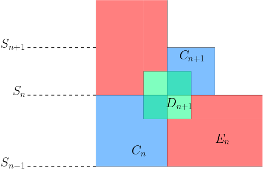
Figure 4: The several areas used to study density $\rho$ in the upper bound of Theorem 2.2.

See fig. 4 for a visual representation. Notice how these three areas cover the whole unit square. Let us check that $\rho$ is small outside the diagonal neighborhood $C\cup D$:

$$\text{for all }n\in\mathbb{N}^{*}\text{ and }(x,y)\in E_{n},\quad|x-y|\geq u_{n+1}/2\quad\text{and}\quad R_{n}\leq\mathrm{dist}\big{(}(x,y),(1,1)\big{)}\leq 2R_{n-1}.$$

Then using Lemma 4.2, we get as $n\rightarrow\infty$ uniformly in $(x,y)\in E_{n}$:

$$|x-y|=\Omega\left(n^{-\beta}\log(n)^{\gamma}\right)\quad\text{and}\quad\mathrm{dist}\big{(}(x,y),(1,1)\big{)}=\Theta\left(n^{1-\beta}\log(n)^{\gamma}\right).$$

Our hypothesis on $\rho$ now rewrites

$$\rho(x,y) =O\left(\left(n^{1-\beta}\log(n)^{\gamma}\right)^{\frac{\beta}{1-\beta}}\exp\left(-\Omega\left(n^{-\beta}\log(n)^{\gamma}\left(n^{1-\beta}\log(n)^{\gamma}\right)^{\frac{\beta}{1-\beta}}\right)\right)\right)$$

$$=O\left(n^{\beta}\log(n)^{\frac{\gamma\beta}{1-\beta}}\exp\left(-\Omega\left(\log(n)^{\frac{\gamma}{1-\beta}}\right)\right)\right)$$

$$=o(1)$$

since $\frac{\gamma}{1-\beta}>1$ by choice of $\gamma$. In particular $\rho$ is bounded on $E$, and it reminds to study it on areas $C$ and $D$. Using Lemma 4.2 and bounding the exponential term by $1$, we get as $n\rightarrow\infty$ uniformly in $(x,y)\in C_{n}\cup D_{n+1}$:

$$\rho(x,y)=O\left(n^{\beta}\log(n)^{\frac{\gamma\beta}{1-\beta}}\right).$$

Consequently

$$\int_{C_{n}}\rho(x,y)dxdy=O\left(n^{-2\beta}\log(n)^{2\gamma}n^{\beta}\log(n)^{\frac{\gamma\beta}{1-\beta}}\right)=O\left(n^{-\beta}\log(n)^{\gamma\left(2-\frac{\beta}{\beta-1}\right)}\right)\quad\text{as }n\rightarrow\infty$$

and likewise

$$\int_{D_{n+1}}\rho(x,y)dxdy=O\left(n^{-\beta}\log(n)^{\gamma\left(2-\frac{\beta}{\beta-1}\right)}\right)\quad\text{as }n\rightarrow\infty.$$

Define $\gamma^{\prime}:=\gamma\left(2-\frac{\beta}{\beta-1}\right)>0$. The previous calculations show that we can find a bound

$$\rho\leq M(f+g+h)$$

for some $M>0$, $f$ the uniform density on $[0,1]^{2}$, $g$ a probability density on $C$ attributing uniform mass proportionnal to $n^{-\beta}\log(n+1)^{\gamma^{\prime}}$ to each $C_{n}$, and $h$ a probability density on $D$ attributing uniform mass proportionnal to $n^{-\beta}\log(n+1)^{\gamma^{\prime}}$ to each $D_{n+1}$. Thus by Lemma 3.2 it suffices to bound the quantities

$$\mathbb{E}\left[\mathrm{LIS}\big{(}\mathrm{Sample}_{N}(\mu_{f})\big{)}\right],\quad\mathbb{E}\left[\mathrm{LIS}\big{(}\mathrm{Sample}_{N}(\mu_{g})\big{)}\right],\quad\mathbb{E}\left[\mathrm{LIS}\big{(}\mathrm{Sample}_{N}(\mu_{h})\big{)}\right].$$

The first term is nothing but the uniform case, so behaves as $\Theta\left(\sqrt{N}\right)$. Let us turn to the second term. Since the sampled permutations of our reference permutons only depend on the masses attributed to each box and not the sizes of these boxes, sampled permutations from $\mu_{g}$ have the same law as sampled permutations from $\mu_{\beta,\gamma^{\prime}}^{\nearrow}$ (see Section 2.4; $\mu_{\beta,\gamma^{\prime}}^{\nearrow}$ is the permuton associated to the pre-permuton $\mu_{g}$). Hence by 2.3, this term behaves as $\widetilde{\Theta}\left(N^{1/\beta}\right)$. The third term is handled the same way. Finally:

$$\mathbb{E}\left[\mathrm{LIS}\big{(}\mathrm{Sample}_{N}(\mu_{\rho})\big{)}\right]=\underset{N\rightarrow\infty}{\widetilde{O}}\left(N^{1/\beta}\right).$$

5.3 Proof of Theorem 2.1

This section is devoted to the proof of Theorem 2.1. We thus consider $\alpha>-2$ and suppose $\rho$ is as in the theorem. Since we want an upper bound on the longest increasing subsequences, we need to find appropriate areas to bound $\rho$ on. For this define $\beta>1$ by

$$-\alpha=2-\frac{1}{\beta-1}\quad\textit{i.e.}\quad\alpha(1-\beta)+1-2\beta=-2.$$ (12)

We use the notation of Section 2.2 for this value of $\beta$ and $\gamma=0$. We shall bound $\rho$ on the boxes $(C_{n})_{n\in\mathbb{N}^{*}}$ as well as on the adjacent rectangles:

$$\text{for all }n\in\mathbb{N}^{*},\quad D_{n}^{(1)}:=[S_{n-1},S_{n}]\times[S_{n},1]\quad\text{and}\quad D_{n}^{(2)}:=[S_{n},1]\times[S_{n-1},S_{n}].$$

The sequences $(C_{n})_{n\in\mathbb{N}^{*}},(D_{n}^{(1)})_{n\in\mathbb{N}^{*}},(D_{n}^{(2)})_{n\in\mathbb{N}^{*}}$ form a partition of the unit square. As in the upper bound of Theorem 2.2, we need to compute the masses attributed by $\rho$ to each of these boxes. For this notice that

$$\text{for all }n\in\mathbb{N}^{*}\text{ and }(x,y)\in C_{n}\cup D_{n}^{(1)}\cup D_{n}^{(2)},\quad R_{n}\leq\mathrm{dist}((x,y),(1,1))\leq 2R_{n-1}.$$

Hence

$$\int_{C_{n}}\rho(x,y)dxdy=\underset{}{\Theta}\left(n^{\alpha(1-\beta)}n^{-2\beta}\right)=\underset{}{\Theta}\left(n^{-3}\right)\quad\text{as }n\rightarrow\infty$$

and

$$\text{for }i=1,2,\quad\int_{D_{n}^{(i)}}\rho(x,y)dxdy=\underset{}{\Theta}\left(n^{\alpha(1-\beta)}n^{-\beta}n^{1-\beta}\right)=\underset{}{\Theta}\left(n^{-2}\right)\quad\text{as }n\rightarrow\infty$$

by eq. 12. Using Lemma 3.2, it suffices to bound the quantities

$$\mathbb{E}\left[\mathrm{LIS}\big{(}\mathrm{Sample}_{N}(\mu_{f})\big{)}\right],\quad\mathbb{E}\left[\mathrm{LIS}\big{(}\mathrm{Sample}_{N}(\mu_{g})\big{)}\right],\quad\mathbb{E}\left[\mathrm{LIS}\big{(}\mathrm{Sample}_{N}(\mu_{h})\big{)}\right]$$

where $f$ is the probability density on $C$ attributing uniform mass proportional to $n^{-3}$ to each $C_{n}$ and $g$ (resp. $h$) is the probability density on $D^{(1)}$ (resp. $D^{(2)}$) attributing uniform mass proportional to $n^{-2}$ to each $D_{n}^{(1)}$ (resp. $D_{n}^{(2)}$). Considering the reference permuton $\mu_{3}^{\nearrow}$ of parameter $(3,0)$, 2.3 tells us

$$\mathbb{E}\left[\mathrm{LIS}\left(\mathrm{Sample}_{N}(\mu_{3}^{\nearrow})\right)\right]=\underset{N\rightarrow\infty}{\widetilde{\Theta}}\left(\sqrt{N}\right).$$

Since $\mu_{3}^{\nearrow}$ attributes the same masses to the boxes of its support as density $f$ attributes to its own, sampled permutations from both pre-permutons have same law (the same remark as in the upper bound of Theorem 2.2 holds; $\mu_{3}^{\nearrow}$ is the permuton associated to the pre-permuton $\mu_{f}$). Consequently:

$$\mathbb{E}\left[\mathrm{LIS}\left(\mathrm{Sample}_{N}(\mu_{f}^{\nearrow})\right)\right]=\underset{N\rightarrow\infty}{\widetilde{\Theta}}\left(\sqrt{N}\right).$$

The case of density $g$ is similar but with a slight alteration. Indeed, considering the reference permuton $\mu_{2}^{\nearrow}$ of parameter $(2,0)$, 2.3 tells us

$$\mathbb{E}\left[\mathrm{LIS}\left(\mathrm{Sample}_{N}(\mu_{2}^{\nearrow})\right)\right]=\underset{N\rightarrow\infty}{\widetilde{\Theta}}\left(\sqrt{N}\right).$$ (13)

Note that $\mu_{2}^{\nearrow}$ attributes the same masses to the boxes of its support as density $g$ attributes to its own. A key difference here is that the rectangle boxes $D_{n}^{(1)}$ are not placed increasingly inside the unit square, so sampled permutations from permuton $\mu_{2}^{\nearrow}$ and density $g$ do not have the same law. To work around this problem, we can use an appropriate coupling. Take random i.i.d. points $X_{1},\dots,X_{N}$ distributed under density $g$. Consider, for each $n\in\mathbb{N}^{*}$, the affine transformation $a_{n}$ mapping $D_{n}^{1}$ to $C_{n}$ and assemble them into a function $a$ from $\cup_{n\geq 1}D_{n}^{1}$ to $\cup_{n\geq 1}C_{n}$. Then the image points $a(X_{1}),\dots,a(X_{N})$ are i.i.d. under the measure $\mu_{2}^{\nearrow}$. Moreover, each increasing subset of $\{X_{1},\dots,X_{N}\}$ is mapped to an increasing subset of $\{a(X_{1}),\dots,a(X_{N})\}$. This coupling argument shows that $\mathrm{LIS}\big{(}\mathrm{Sample}_{N}(\mu_{g})\big{)}$ is stochastically dominated by $\mathrm{LIS}\big{(}\mathrm{Sample}_{N}(\mu_{2}^{\nearrow})\big{)}$, and eq. 13 then implies:

$$\mathbb{E}\left[\mathrm{LIS}\big{(}\mathrm{Sample}_{N}(\mu_{g})\big{)}\right]=\underset{N\rightarrow\infty}{\widetilde{O}}\left(\sqrt{N}\right).$$

Density $h$ is handled the same way. Hence:

$$\mathbb{E}\left[\mathrm{LIS}\big{(}\mathrm{Sample}_{N}(\mu_{\rho})\big{)}\right]=\underset{N\rightarrow\infty}{\widetilde{O}}\left(\sqrt{N}\right).$$

To conclude the proof of Theorem 2.1, the lower bound is obtained as a direct consequence of Lemma 3.1 using the uniform case (see the proof of 3.3).

6 Study of densities diverging along the diagonal

6.1 Lower bound of Theorem 2.4

From now on we consider a density $\rho$ satisfying the hypothesis of Theorem 2.4 for some exponent $\alpha\in]-1,0[$. As explained in Section 2.5, the idea is to slice the unit square into small boxes and investigate the number of sampled points appearing in appropriate increasing sequences of boxes. Let $N\in\mathbb{N}^{*}$ and take random i.i.d. points $X_{1},\dots,X_{N}$ distributed under density $\rho$. Set

$$b_{N}:=\left\lfloor N^{1/(\alpha+2)}\right\rfloor,$$

and define a family of $b_{N}^{2}$ identical boxes by

$$\text{for all }(i,j)\in[\![1,b_{N}]\!]^{2},\quad C_{i,j}:=\left[\frac{(i-1)}{b_{N}},\frac{i}{b_{N}}\right]\times\left[\frac{(j-1)}{b_{N}},\frac{j}{b_{N}}\right].$$

This covering of the unit square will be useful for the upper bound, while the lower bound aimed for in this section only requires using the increasing sequence of boxes $(C_{k,k})_{k\in[\![1,b_{N}]\!]}$. More precisely, we make use of the inequality

$$\mathrm{LIS}(X_{1},\dots,X_{N})\geq\sum_{k=1}^{b_{N}}\mathbf{1}_{N_{k}\geq 1}$$ (14)

where each $N_{k}$ denotes the number of points among $X_{1},\dots,X_{N}$ in $C_{k,k}$. Thanks to the hypothesis made on $\rho$, we can fix $\delta,\varepsilon>0$ such that

$$\text{for all }(x,y)\in[0,1]^{2}\text{ satisfying }|x-y|<\delta,\quad\rho(x,y)\geq\varepsilon|x-y|^{\alpha}.$$

Now suppose $N$ is big enough to have $b_{N}^{-1}<\delta$ and compute, for any $k\in[\![1,b_{N}]\!]$:

$$m_{k}:=\iint_{C_{k,k}}\rho(x,y)dxdy\geq\iint_{C_{k,k}}\varepsilon|x-y|^{\alpha}dxdy=\varepsilon\int_{0}^{b_{N}^{-1}}dx\int_{-x}^{b_{N}^{-1}-x}dz|z|^{\alpha}\\ =\varepsilon\int_{0}^{b_{N}^{-1}}dx\left(\frac{x^{\alpha+1}}{\alpha+1}+\frac{(b_{N}^{-1}-x)^{\alpha+1}}{\alpha+1}\right)=\frac{2\varepsilon}{(\alpha+1)(\alpha+2)}b_{N}^{-(\alpha+2)}=\underset{N\rightarrow\infty}{\Omega}\left(\frac{1}{N}\right).$$

Hence there exists $\eta>0$ satisfying:

$$\text{for all }N\in\mathbb{N}^{*}\text{ and }k\in[\![1,b_{N}]\!],\quad m_{k}\geq\frac{\eta}{N}.$$

Since $N_{k}$ follows a binomial law of parameter $(N,m_{k})$, we thus have :

$$\mathbf{P}(N_{k}=0)=(1-m_{k})^{N}\leq(1-\eta/N)^{N}\underset{N\rightarrow\infty}{\longrightarrow}e^{-\eta}<1.$$

Consequently there exists a constant $p_{0}>0$ such that

$$\text{for any big enough }N\in\mathbb{N}^{*}\text{ and all }k\in[\![1,b_{N}]\!],\quad\mathbf{P}(N_{k}\geq 1)\geq p_{0}.$$

Hence for big enough $N$, using eq. 14 :

$$\mathbb{E}\left[\mathrm{LIS}\big{(}\mathrm{Sample}_{N}(\mu_{\rho})\big{)}\right]\geq\mathbb{E}\left[\sum_{k=1}^{b_{N}}\mathbf{1}_{N_{k}\geq 1}\right]\geq\sum_{k=1}^{b_{N}}p_{0}=p_{0}b_{N}=\underset{N\rightarrow\infty}{\Omega}\left(N^{1/(\alpha+2)}\right).$$

6.2 Upper bound of Theorem 2.4

We use the same notation as in last section, but this time we investigate the whole grid $(C_{i,j})_{i,j\in[\![1,b_{N}]\!]}$. Say a sequence of distinct boxes

$$\mathcal{C}=(C_{i_{1},j_{1}},\dots,C_{i_{n},j_{n}})$$

is increasing whenever

$$\text{for all }k\in[\![1,n-1]\!],\quad i_{k}\leq i_{k+1}\text{ and }j_{k}\leq j_{k+1}.$$

When this happens, one has $n<2b_{N}$. Indeed, when browsing the sequence, each coordinate increases at most $b_{N}-1$ times. Write

$$\mathcal{X}:=\{X_{1},\dots,X_{N}\}.$$

Then, for any box $C$, denote by $\mathcal{X}_{C}$ the set of points in $\mathcal{X}$ appearing in $C$ and, for any increasing sequence of boxes $\mathcal{C}$, denote by $\mathcal{X}_{\mathcal{C}}$ the set of points in $\mathcal{X}$ appearing in some box of $\mathcal{C}$. We aim to make use of the inequality

$$\mathrm{LIS}(\mathcal{X})\leq\sup_{\mathcal{C}\text{ increasing sequence of boxes}}|\mathcal{X}_{\mathcal{C}}|$$ (15)

since the family of boxes occupied by an increasing subset of points necessarily rearranges as an increasing sequence of boxes. Now, thanks to the hypothesis made on $\rho$, let $M>0$ be such that

$$\text{for all }(x,y)\in[0,1]^{2},\quad\rho(x,y)\leq M|x-y|^{\alpha}.$$

Since this latter function puts more mass on the diagonal boxes than the outside ones, we have:

$$\text{for any }(i,j)\in[\![1,b_{N}]\!]^{2},\quad\iint_{C_{i,j}}\rho(x,y)dxdy\leq\iint_{C_{i,j}}M|x-y|^{\alpha}dxdy\\ \leq M\int_{0}^{b_{N}^{-1}}\int_{0}^{b_{N}^{-1}}|x-y|^{\alpha}dxdy=\frac{2M}{(\alpha+1)(\alpha+2)}b_{N}^{-(\alpha+2)}=\underset{N\rightarrow\infty}{O}(1/N).$$

Thus there exists $M^{\prime}>0$ such that, for big enough $N$, each variable $|\mathcal{X}_{C_{i,j}}|$ is stochastically dominated by the law $\mathrm{Bin}(N,M^{\prime}/N)$. Additionally Lemma 4.1 gives, denoting by $\mathcal{S}_{N}$ a random variable of law $\mathrm{Bin}(N,M^{\prime}/N)$:

$$\mathbf{P}\left(\left|\mathcal{S}_{N}-M^{\prime}\right|\geq\log(N)^{2}\sqrt{M^{\prime}}\right)\leq 2\exp\left(-\psi_{N}\right)$$

$$\text{where}\quad\psi_{N}=\frac{\log(N)^{4}M^{\prime}/2}{M^{\prime}(1-M^{\prime}/N)+\log(N)^{2}\sqrt{M^{\prime}}/3}=\underset{N\rightarrow\infty}{\Theta}(\log(N)^{2}).$$

This inequality, along with the aforementioned stochastic domination, implies that for big enoug $N$:

$$\mathbf{P}\left(\forall(i,j),\;|\mathcal{X}_{C_{i,j}}|\leq M^{\prime}+\log(N)^{2}\sqrt{M^{\prime}}\right)\geq 1-2b_{N}^{2}\exp(-\psi_{N}).$$

Hence, using the fact that an increasing sequence of boxes contains at most $2b_{N}$ boxes:

$$\mathbf{P}\left(\text{for any increasing sequence of boxes }\mathcal{C},\;|\mathcal{X}_{\mathcal{C}}|\leq 2b_{N}\left(M^{\prime}+\log(N)^{2}\sqrt{M^{\prime}}\right)\right)\geq 1-2b_{N}^{2}\exp(-\psi_{N})$$

and then, by eq. 15:

$$\mathbf{P}\left(\mathrm{LIS}(\mathcal{X})\leq 2b_{N}\left(M^{\prime}+\log(N)^{2}\sqrt{M^{\prime}}\right)\right)\geq 1-2b_{N}^{2}\exp(-\psi_{N}).$$

To conclude the proof of Theorem 2.4, it suffices to write:

$$\mathbb{E}\left[\mathrm{LIS}\big{(}\mathrm{Sample}_{N}(\mu_{\rho})\big{)}\right]\leq 2b_{N}\left(M^{\prime}+\log(N)^{2}\sqrt{M^{\prime}}\right)+2b_{N}^{2}N\exp(-\psi_{N})=\widetilde{O}\left(N^{1/(\alpha+2)}\right).$$

7 Acknowledgements

I would like to express my sincere thanks to Valentin Féray for his constant support and enlightening discussions, as well as all members of IECL who contribute to a prosperous environment for research in mathematics.

References

• [AD95] David J. Aldous and Persi Diaconis. Hammersley’s interacting particle process and longest increasing subsequences. Probability Theory and Related Fields, 103:199–213, 1995.
• [Azu67] Kazuoki Azuma. Weighted sums of certain dependent random variables. Tohoku Mathematical Journal, 19:357–367, 1967.
• [BBD+22] Frédérique Bassino, Mathilde Bouvel, Michael Drmota, Valentin Féray, Lucas Gerin, Mickaël Maazoun, and Adeline Pierrot. Linear-sized independent sets in random cographs and increasing subsequences in separable permutations. Combinatorial Theory, 2, 2022.
• [BBF+18] Frédérique Bassino, Mathilde Bouvel, Valentin Féray, Lucas Gerin, and Adeline Pierrot. The Brownian limit of separable permutations. The Annals of Probability, 46(4):2134 – 2189, 2018.
• [BBF+20] Frédérique Bassino, Mathilde Bouvel, Valentin Féray, Lucas Gerin, Mickaël Maazoun, and Adeline Pierrot. Universal limits of substitution-closed permutation classes. Journal of the European Mathematical Society, 22(11):3565–3639, 2020.
• [BBF+22] Frédérique Bassino, Mathilde Bouvel, Valentin Féray, Lucas Gerin, Mickaël Maazoun, and Adeline Pierrot. Scaling limits of permutation classes with a finite specification: A dichotomy. Advances in Mathematics, 405:108513, 2022.
• [BDJ99] Jinho Baik, Percy Deift, and Kurt Johansson. On the distribution of the length of the longest increasing subsequence of random permutations. Journal of the American Mathematical Society, 12(4):1119–1178, 1999.
• [BDMW22] Jacopo Borga, Sayan Das, Sumit Mukherjee, and Peter Winkler. Large deviation principle for random permutations, 2022. preprint arXiv:2206.04660v1.
• [Ben62] George Bennett. Probability inequalities for the sum of independent random variables. Journal of the American Statistical Association, 57(297):33–45, 1962.
• [Ber27] Sergueï Natanovitch Bernstein. Probability theory, moscow. GOS. Publishing house, 15:83, 1927.
• [DHM15] Martin Doležal, Jan Hladky, and András Máthé. Cliques in dense inhomogeneous random graphs. Random Structures and Algorithms, 51:275–314, 2015.
• [Dub23] Victor Dubach. Increasing subsequences of linear size in random permutations. in preparation, 2023.
• [DZ95] Jean-Dominique Deuschel and Ofer Zeitouni. Limiting curves for i.i.d. records. The Annals of Probability, 23(2):852 – 878, 1995.
• [Fri98] Alan Frieze. On the length of the longest monotone subsequence in a random permutation. The Annals of Applied Probability, 1(2):301–305, 1998.
• [GGKK15] Roman Glebov, Andrzej Grzesik, Tereza Klimošová, and Daniel Král’. Finitely forcible graphons and permutons. Journal of Combinatorial Theory, Series B, 110:112–135, 2015.
• [HKM+13] Carlos Hoppen, Yoshiharu Kohayakawa, Carlos Gustavo Moreira, Balázs Ráth, and Rudini Menezes Sampaio. Limits of permutation sequences. Journal of Combinatorial Theory, Series B, 103(1):93–113, 2013.
• [Hoe63] Wassily Hoeffding. Probability inequalities for sums of bounded random variables. Journal of the American Statistical Association, 58(301):13–30, 1963.
• [Kiw06] Marcos Kiwi. A concentration bound for the longest increasing subsequence of a randomly chosen involution. Discrete Applied Mathematics, 154(13):1816–1823, 2006.
• [KP13] Daniel Král and Oleg Pikhurko. Quasirandom permutations are characterized by 4-point densities. Geometric and Functional Analysis, 23:570–579, 2013.
• [McD89] Colin McDiarmid. On the method of bounded differences. London Mathematical Society Lecture Note Series. Cambridge University Press, 1989.
• [McK19] Gweneth McKinley. Superlogarithmic cliques in dense inhomogeneous random graphs. SIAM Journal on Discrete Mathematics, 33(3):1772–1800, 2019.
• [Muk15] Sumit Mukherjee. Fixed points and cycle structure of random permutations. Electronic Journal of Probability, 21:1–18, 2015.
• [Rom15] Dan Romik. The Surprising Mathematics of Longest Increasing Subsequences. Institute of Mathematical Statistics Textbooks (4). Cambridge University Press, 2015.
• [Sjö22] Jonas Sjöstrand. Monotone subsequences in locally uniform random permutations, 2022. preprint arXiv:2207.11505.
• [Tal95] Michel Talagrand. Concentration of measure and isoperimetric inequalities in product spaces. Publications mathématiques de l’IHÉS, 81:73–205, 1995.
• [VK77] Anatoli Vershik and Sergueï Kerov. Asymptotics of the plancherel measure of the symmetric group and the limit form of young tableaux sov. Methods Dokl, 18:527531, 1977.