Non-parametric identifiability and sensitivity analysis of synthetic control models

Abstract

Quantifying cause and effect relationships is an important problem in many domains. The gold standard solution is to conduct a randomised controlled trial. However, in many situations such trials cannot be performed. In the absence of such trials, many methods have been devised to quantify the causal impact of an intervention from observational data given certain assumptions. One widely used method are synthetic control models. While identifiability of the causal estimand in such models has been obtained from a range of assumptions, it is widely and implicitly assumed that the underlying assumptions are satisfied for all time periods both pre- and post-intervention. This is a strong assumption, as synthetic control models can only be learned in pre-intervention period. In this paper we address this challenge, and prove identifiability can be obtained without the need for this assumption, by showing it follows from the principle of invariant causal mechanisms. Moreover, for the first time, we formulate and study synthetic control models in Pearl’s structural causal model framework. Importantly, we provide a general framework for sensitivity analysis of synthetic control causal inference to violations of the assumptions underlying non-parametric identifiability. We end by providing an empirical demonstration of our sensitivity analysis framework on simulated and real data in the widely-used linear synthetic control framework.

1 Introduction

Understanding and quantifying cause and effect relationships is a fundamental problem in numerous domains, from science to medicine and economics—see [Gilligan-Lee(2020), Richens et al.(2020)Richens, Lee, and Johri, Lee and Spekkens(2017), Jeunen et al.(2022)Jeunen, Gilligan-Lee, Mehrotra, and Lalmas, Dhir and Lee(2020), Reynaud et al.(2022)Reynaud, Vlontzos, Dombrowski, Lee, Beqiri, Leeson, and Kainz, Gilligan-Lee et al.(2022)Gilligan-Lee, Hart, Richens, and Johri, Perov et al.(2020)Perov, Graham, Gourgoulias, Richens, Lee, Baker, and Johri, Vlontzos et al.(2021)Vlontzos, Kainz, and Gilligan-Lee]. The generally-accepted gold standard solution to this problem is to conduct a randomised controlled trial, or A/B test. However, in many situations such trials cannot be performed; they could be unethical, exorbitantly expensive, or technologically infeasible. In the absence of such trials, many methods have been developed to infer the causal impact of an intervention or treatment from observational data given certain assumptions. One of the most widely used causal inference approaches in economics [Abadie et al.(2010)Abadie, Diamond, and Hainmueller], marketing [Brodersen et al.(2015)Brodersen, Gallusser, Koehler, Remy, Scott, et al.], and medicine [Kreif et al.(2016)Kreif, Grieve, Hangartner, Turner, Nikolova, and Sutton] are synthetic control methods.

To concretely illustrate synthetic controls, consider the launch of an advertising campaign in a specific geographic region, aimed to increase sales of a product there. To estimate the impact of this campaign, the synthetic control method uses the number of sales of the product in different regions, where no policy change was implemented, to build a model which predicts the pre-campaign sales in the campaign region. This model is then used to predict product sales in the campaign region in the counterfactual world where no advertising campaign was launched. By comparing the model prediction to actual sales in that region after the campaign was launched, one can estimate its impact.

In the standard synthetic control set-up, the model is taken to be a weighted, linear combination of sales in the no-campaign regions. To train the model, one needs to determine the weights for sales in each no-campaign region that minimise the error when predicting the sales in the campaign region before the campaign was launched. The linearity of the model is justified by assuming an underlying linear factor model for all regions, or units, that is the same for all time periods, both before and after the intervention. Recent work by [Shi et al.(2022)Shi, Sridhar, Misra, and Blei] has removed the need for the linear factor model assumption and proven identifiability from a non-parametric assumption: that units are aggregates of smaller units. This assumption is reasonable in situations like our advertising campaign example, where total sales in a region is just the aggregate of sales from each individual in that region. However, in many applications, this assumption does not apply. In medicine for instance, patients are not generally considered to be aggregates of smaller units. When the aggregate unit assumption can’t be justified, can the causal effect of an intervention on a specific unit be identified from data about “similar” units not impacted by the intervention?

Returning to our example, the reason sales in different regions provide good synthetic control candidates is that the causes of sales in most regions are very similar, consisting of demographic factors, socioeconomic status of residents, and so on. Informally, sales in “similar” regions act as proxies for these, generally unobserved, causes of sales in the campaign region. That is, before the campaign, the causes of sales in the campaign region are also causes of sales in the no-campaign region—they are common causes of the campaign and no-campaign regions. This relationship between the target variable and synthetic control candidates is illustrated as a directed acyclic graph, or DAG, in Figure 1. [Shi et al.(2021b)Shi, Miao, Hu, and Tchetgen Tchetgen] combined this formulation with results from the proximal causal inference literature to prove one can identify the causal effect of an intervention on the target unit from data about the proxy units not impacted by the intervention. See [Tchetgen et al.(2020)Tchetgen, Ying, Cui, Shi, and Miao] for an overview of proximal causal inference. Hence, in our example, observing sales in multiple no-campaign regions allows one to predict the contemporaneous evolution of sales in the campaign region in the absence of the campaign without needing any linearity assumptions.

However, in all previous identifiability proofs, it is implicitly assumed that the underlying assumptions are satisfied for all time periods, both pre- and post-intervention (see assumption 3” in [Shi et al.(2021b)Shi, Miao, Hu, and Tchetgen Tchetgen], and assumption A2 in [Shi et al.(2022)Shi, Sridhar, Misra, and Blei]). This is a strong assumption, as models can only be learned in pre-intervention period. That is, one of the main assumptions underlying the validity of synthetic control models is that there is no unobserved heterogeneity in the relationship between the target and the control time-series observed in the pre-intervention period. Such unobserved heterogeneity could, for instance, be due to unaccounted-for causes of the target unit.

In this paper we address this challenge, and prove identifiability can be obtained without the need for the requirement that assumptions hold for all time periods before and after the intervention, by proving it follows from the principle of invariant causal mechanisms. Moreover, for the first time, we formulate and study synthetic control models in Pearl’s structural causal model framework.

As the assumptions underlying our identifiability proof cannot be empirically tested—as with all causal inference results—it is vital to conduct a formal sensitivity analysis to determine robustness of the causal estimate to violations of these assumptions. In propensity-based causal inference for instance, sensitivity analysis has been conducted to determine how robust propensity-based causal estimates are to the presence of unobserved confounders, see [Veitch and Zaveri(2020)] for an overview. These sensitivity analyses derived a relationship between the influence of unobserved confounders and the resulting bias in causal effect estimation. This understanding allows one to bound bias in causal effect estimation as a function of unobserved confounder influence. From this a domain expert can offer judgments of the bias due to plausible levels of unobserved confounding.

However, despite the importance of this problem—and the wide use of synthetic control methods in many disciplines—general methods for sensitivity analysis of synthetic control methods are under-studied. This work’s contributions seek to remedy this discrepancy and provide a general framework for sensitivity analysis of synthetic control causal inference to violations of the assumptions underlying our non-parametric identifiability proof.

In summary, our main contributions are as follows:

1. We formulate synthetic control models in Pearl’s structural causal model framework.

2. We provide a non-parametric identifiability proof in Pearl’s structural causal model framework that doesn’t require assumptions to be satisfied before and after the intervention. Our proof relies on the invariant causal mechanism principle.

3. We provide a general framework for sensitivity analysis of synthetic control causal inference to violations of the assumptions underlying our non-parametric identifiability proof.

4. We empirically demonstrate our sensitivity analysis approach on real-world data.

Paper Organisation

As discussed in the introduction, our goal is to identify the causal effect of an intervention, or treatment, on the unit to which it was applied using data from “similar” units not impacted by the treatment. First we overview related work, then formulate synthetic control models in Pearl’s structural causal model framework, where we prove identifiability using results from proximal causal inference and the assumption that causal mechanisms are invariant. Finally, we provide a formal sensitivity analysis when the assumptions of our identifiability proof fail.

2 Related work

Identifiability of synthethic controls

The standard approach to synthetic control models uses the assumption that the data is generated by an underlying linear factor model to derive prove the counterfactual is identified as a linear combination of units not impacted by the treatment, see [Abadie and Gardeazabal(2003), Abadie et al.(2010)Abadie, Diamond, and Hainmueller]. Recent work in [Shi et al.(2022)Shi, Sridhar, Misra, and Blei] proved that this linearity emerges in a non-parametric manner if treatment and control units are coarse-grainings of “smaller” units, and if causal mechanisms are independent. Recent work by [Shi et al.(2021b)Shi, Miao, Hu, and Tchetgen Tchetgen], removed the need for this “aggregate unit” assumption, and proved that the counterfactual can be identified as a function of the control units—but this function need not be linear. The result of [Shi et al.(2021b)Shi, Miao, Hu, and Tchetgen Tchetgen] uses tools from the proximal causal inference literature, see [Tchetgen et al.(2020)Tchetgen, Ying, Cui, Shi, and Miao] for an overview. Initial proximal causal inference results were reported in [Kuroki and Pearl(2014), Miao et al.(2018)Miao, Geng, and Tchetgen Tchetgen], and have since been developed further and used in long-term causal effect estimation [Imbens et al.(2022)Imbens, Kallus, Mao, and Wang]. See [Shpitser et al.(2021)Shpitser, Wood-Doughty, and Tchetgen] for a formulation of proximal causal inference in the graphical causal inference framework. We note that all the aforementioned works are formulated in the potential outcomes framework for causal inference. Moreover, as mentioned previously, in all these works it is taken that the underlying assumptions are satisfied for all time periods. This is a strong assumption, as models can only be learned in pre-treatment period.

Invariant causal mechanisms

As mentioned, in this paper we prove identifiability can be obtained without the need for this assumption, by showing it follows from the principle of invariant causal mechanisms.Causal mechanisms are invariant if they take the same form in different domains, even though the data distributions may vary with domain. Previous work on invariant causal mechanisms can be found in [Mitrovic et al.(2020)Mitrovic, McWilliams, Walker, Buesing, and Blundell, Guo et al.(2022)Guo, Tóth, Schölkopf, and Huszár, Wang et al.(2022)Wang, Yi, Chen, and Zhu, Chevalley et al.(2022)Chevalley, Bunne, Krause, and Bauer]. Importantly, this principle is related—yet distinct from—the principle of independent causal mechanisms, which says that the mechanism that maps a cause to its effect is independent of the distribution of the cause in a given domain [Parascandolo et al.(2018)Parascandolo, Kilbertus, Rojas-Carulla, and Schölkopf, Stegle et al.(2010)Stegle, Janzing, Zhang, Mooij, and Schölkopf]. In the independent causal mechanism principle, the mechanism itself need not be the same across domains, it just cannot contain information about the distribution of the cause.

Sensitivity analsysis

Later in the paper, we use our identifiability proof to formally investigate synthetic control models from a sensitivity analysis standpoint for the first time. Previous work on sensitivity analysis has investigated omitted variable bias in propensity-based models. This sensitivity analysis work originated in [Imbens(2003), Rosenbaum and Rubin(1983)] with modern extensions in [Veitch and Zaveri(2020)] and [Cinelli and Hazlett(2020), Cinelli et al.(2019)Cinelli, Kumor, Chen, Pearl, and Bareinboim].

3 Methods

3.1 Non-parametric identifiability from proxies and invariant causal mechanisms

[ ]  [ ]

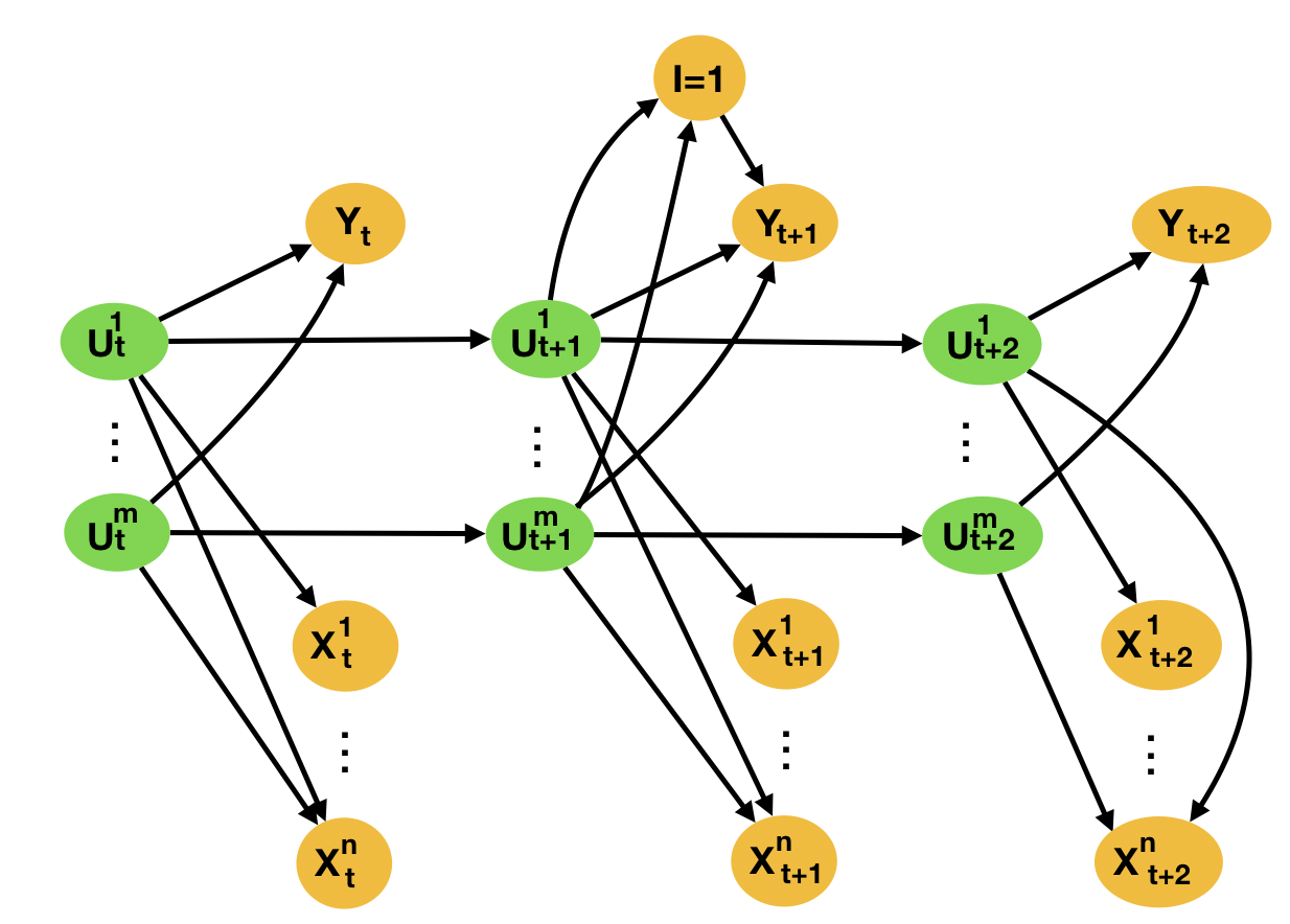
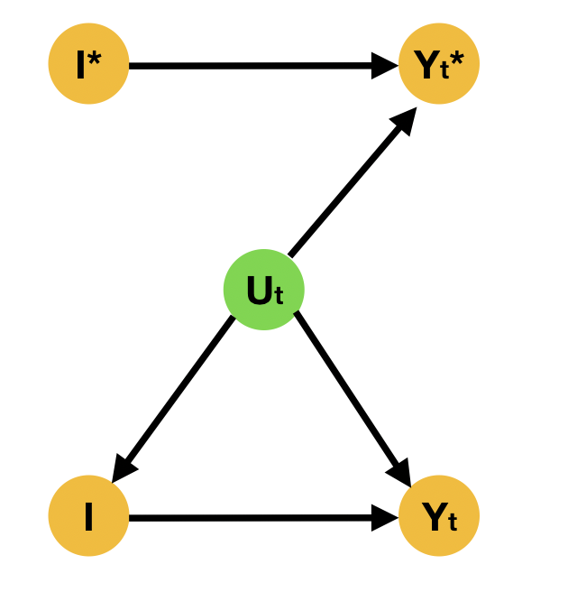
Figure 1: (a) DAG for synthetic control method. Orange nodes are observed variables, green latent. Intervention is applied at timepoint $t+1$. For simplicity, $I$ is taken to be $0$ for all time points before $t+1$, and $1$ for all timepoints from $t+1$ on-wards. (b) Twin network for target unit. Superscript ^∗ denotes counterfactual world.

We work in the structural causal model framework of [Pearl(2009)]. We now will present our definition of a synthetic control structural causal model, define invariant causal mechanisms, and formally define proxy variables following the proximal causal inference literature of [Tchetgen et al.(2020)Tchetgen, Ying, Cui, Shi, and Miao].

Definition 3.1 (Synthetic Control Structural Causal Model )

A synthetic control structural causal model consists of a set of latent variables $U$ and their distributions, a set of observed variables $\mathbf{Y,X,I}$ representing the target unit, donor units, and the intervention, and a set of deterministic functions mapping parents to their children in the causal structure in Figure 1(a), represented as a directed acyclic graph (DAG), each indexed by a specific time point $t$, such that:

1. $u^{t}=m^{t}(u^{t-1},\epsilon^{t}_{u})$ where $\epsilon^{t}_{u}$ is an independent, exogenous error term with $\epsilon^{t}_{u}\sim P(\epsilon^{t}_{u})$

2. $y^{t}=g^{t}(u^{t},I^{t},\epsilon^{t}_{y})$ where $\epsilon^{t}_{u}$ is an independent, exogenous error term with $\epsilon^{t}_{y}\sim P(\epsilon^{t}_{y})$

3. $x^{t}_{i}=f^{t}(u^{t},\epsilon^{t}_{x_{i}})$ where $\epsilon^{t}_{x_{i}}$ is an independent, exogenous error term with $\epsilon^{t}_{u}\sim P(\epsilon^{t}_{x_{i}})$

For simplicity, we follow [Zhang and Bareinboim(2022)] and suppress the functional dependence on the exogenous error terms.

The above formulation in terms of structural causal models generalises the standard formulation of synthetic controls in terms of linear factor models. For instance, $y^{t}$ is considered an arbitrary function of $u^{t},I^{t}$, rather than a linear function of them. In what follows we treat $x^{t},y^{t}$ as the variables we are concerned with. Sometimes we abuse notation and use the same $x^{t},y^{t}$ to denote the values those variables take. The difference will be clear from the context.

The collection of functions and distribution over latent variables induces a distribution over observable variables: $P^{t}(x^{t})=\sum_{u^{t}}P^{t}(x^{t}\mid u^{t})P^{t}(u^{t})=\sum_{u^{t}}\delta_{f^{t}(u^{t})=x^{t}}P^{t}(u^{t}).$ Where $\delta_{f^{t}(u^{t})=x^{t}}=1$ when $u^{t}$ satisfies $f^{t}(u^{t})=x^{t}$, and $0$ otherwise. For any variable in a causal model, its causal mechanism is the deterministic function that determines it from its parents in the causal structure. This function is equivalent to the conditional distribution of that variable given it’s parents. For instance: $x^{t}=f^{t}(u^{t})\iff P^{t}(x^{t}\mid u^{t})=1.$

Definition 3.2 (Invariant causal mechanisms)

In the context of synthetic control causal models, a causal mechanism is said to be invariant if it doesn’t depend on the time point $t$.

The structural causal model framework allows us to define (strong) interventions via the do-operator, which replaces the original causal mechanism with assignment of that variable to a specific value, disconnecting the intervened variable from its parents in the causal structure [Pearl(2009)].

To formally define when a collection of variables are to be considered proxies for other variables, we need the following completeness condition.

Definition 3.3 (Completeness condition for proxy variables)

For any square integral function $f$, if $\mathbb{E}\left(f(x^{t}_{1},\dots,x^{t}_{N})\mid u^{t}\right)=0$ then $f(x^{t}_{1},\dots,x^{t}_{N})=0$ for any $t$.

This completeness condition characterizes how much “information” the $x^{t}$ have about the $u^{t}$, in the sense that $x^{t}$ have sufficient variability relative to the $u^{t}$—that is, any variation in $u^{t}$ is captured by variation in $x^{t}$. Such completeness conditions are widely assumed in recent proximal causal inference literature [Tchetgen et al.(2020)Tchetgen, Ying, Cui, Shi, and Miao], and under these conditions the $x^{t}$ can be viewed as proxy variables for the latents $u^{t}$.

To quantify the impact of an intervention $I=1$ on unit $y$ at time $t$, we must estimate the effect of treatment on the treated:

$$\underbrace{\mathbb{E}^{t}\left(y^{t}\mid\text{do}(I^{t}=1),I^{t}=1\right)}_{\text{Observed}}-\mathbb{E}^{t}\left(y^{t}\mid\text{do}(I^{t}=0),I^{t}=1\right)$$

As we observe the first term, all that is required is to identify and estimate the second term.

The below Theorem 3.1 and proof is based on Theorem 4 in [Shi et al.(2021a)Shi, Miao, Hu, and Tchetgen]. The main difference is our assumptions and the causal framework we work in. We work in Pearl’s graphical causal model framework, where independence of causal variables follow from graphical conditions in the given causal structure, represented as a DAG. Indeed, even conditional independence of counterfactual variables can be seen to follow from graphical requirements—this time by considering the structure of the twin network associated with the causal structure, see [Vlontzos et al.(2021)Vlontzos, Kainz, and Gilligan-Lee, Graham et al.()Graham, Lee, and Perov] for an overview of twin networks. [Shi et al.(2021a)Shi, Miao, Hu, and Tchetgen] work in the potential outcomes framework, and thus require explicit assumptions for various conditional independence statements. Additionally, Theorem 4 in [Shi et al.(2021a)Shi, Miao, Hu, and Tchetgen] assumed the existence of a function that maps the control units to the target unit that is consistent and unchanged across all time points. We do not make this assumption. Rather in our Theorem 2 we remove this assumption and prove that such a function is the same for all time points if causal mechanisms are invariant.

For simplicity, we will denote the collection of donor units at timepoint $t$, $\{x^{t}_{1},\dots,x^{t}_{N}\}$, by $x^{t}.$

Theorem 3.1

There exists a function $h^{t}$ such that at time point $t$ we have

$$\mathbb{E}\left(y^{t}\mid\text{do}(I^{t}=0),I^{t}=1\right)=\mathbb{E}\left(h^{t}(x^{t},I^{t}=0)\right),$$

where

$$\mathbb{E}\left(y^{t}\mid\text{do}(I^{t}=0),I^{t}=1\right)=\int y^{t}P^{t}\left(y^{t}\mid\text{do}(I^{t}=0),I^{t}=1\right)dy,$$

and

$$\mathbb{E}\left(h^{t}(x^{t},I^{t}=0)\right)=\int h^{t}(x^{t},I^{t}=0)P^{t}\left(x^{t}\right)dx.$$

Proof 3.1.

In general nonparametric models, the completeness condition of Def. 3.3 together with some additional technical conditions (see the appendix for these technical conditions) imply the existence of a function $H^{t}$ such that

$$P^{t}(y^{t}\mid u^{t},I) =\int H^{t}(y^{t},x^{t},I^{t})P^{t}(x^{t}\mid u^{t},I^{t})dx$$ (1)

This implies that

$$\mathbb{E}\left(y^{t}\mid u^{t},I^{t}\right) =\iint y^{t}H^{t}(y^{t},x^{t},I^{t})P^{t}(x^{t}\mid u^{t},I^{t})dydx$$

$$\overset{A}{=}\int{P^{t}(x^{t}\mid u^{t})}\underbrace{\left[\int{y^{t}H^{t}(y^{t},x^{t},I^{t})}dy\right]}_{:=h^{t}(x^{t},I^{t})}dx$$

$$=\int h^{t}(x^{t},I^{t})P^{t}(x^{t}\mid u^{t},I^{t})dx$$

$$\overset{A}{=}\int h^{t}(x^{t},I^{t})P^{t}(x^{t}\mid u^{t},I^{t})dx$$

$$\overset{B}{=}\mathbb{E}\left(h^{t}(x^{t},I^{t})\mid u^{t},I^{t}\right).$$

Where on lines A we use the fact that $x^{t}$ is independent of $I^{t}$ conditioned on $u^{t}$.

Now, consider the following:

$$\mathbb{E}\left(y^{t}\mid u^{t},I^{t}=1,\text{do}(I^{t}=0)\right) \overset{C}{=}\mathbb{E}\left(y^{t}\mid u^{t},I^{t}=0\right)$$

$$\overset{D}{=}\mathbb{E}\left(h^{t}(x^{t},I^{t}=0)\mid u^{t},I^{t}=0\right)$$

$$\overset{E}{=}\mathbb{E}\left(h^{t}(x^{t},I^{t}=0)\mid u^{t}\right)$$

Line C in the above follows from examining the twin network in Figure 1 and applying d-separation. Line D is just the application of line B, above. Line E follows as $x^{t}$ is independent of $I^{t}$ given $u^{t}$. Marginalising over $u^{t}$ yields: $\mathbb{E}\left(y^{t}\mid\text{do}(I^{t}=0),I^{t}=1\right)=\mathbb{E}\left(h^{t}(x^{t},I^{t}=0)\right)$

Theorem 3.1 proved existence of a function mapping control units to the target unit at a given time. We now prove this function is the same for all timepoints if causal mechanisms are invariant.

Theorem 2.

If causal mechanisms are invariant, then there exists a unique function $h$, such that for all time points $t$ we have:

$$\mathbb{E}\left(y^{t}\mid\text{do}(I^{t}=0),I^{t}=1\right)=\mathbb{E}\left(h(x^{t},I^{t}=0)\right)$$

Proof 3.2.

All we need to show is that the solution to the integral equation from Eq. 1 in the proof of Theorem 3.1 for time point $t$ is also a solution for any other time point $t^{\prime}$.

To show this, first reconsider Eq. 1:

$$P^{t}(y^{t}\mid u^{t},I^{t})=\int H^{t}(y^{t},x^{t},I^{t})P^{t}(x^{t}\mid u^{t},I^{t})dx.$$

Consider the left hand side $P^{t}(y^{t}\mid u^{t},I^{t}).$ This is the causal mechanism for determining $y^{t}$. As causal mechanisms are invariant, this means $P^{t}(y^{t}\mid u^{t},I^{t})=P^{t^{\prime}}(y^{t}\mid u^{t},I^{t}).$ Moreover, considering the right hand side of the above Eq. 1, as $x^{t}$ is independent of $I^{t}$ conditioned on $u^{t}$: $P^{t}(x^{t}\mid u^{t},I^{t})=P^{t}(x^{t}\mid u^{t}),$ which is the causal mechanism for determining $x^{t}$. Again, as causal mechanisms are invariant, one has that $P^{t}(x^{t}\mid u_{t})=P^{t^{\prime}}(x^{t}\mid u^{t}).$

Hence a solution to the integral equation for one time point $t$, is a solution for any other time point $t^{\prime}$. All that remains is to prove uniqueness of $h^{t}$ for a given time point, as this will imply there exists a unique function $h$ for all time points via the above argument. Suppose there are two functions that are each solutions to line E: $\mathbb{E}\left(h^{t}(x^{t},I^{t})\mid u^{t},I^{t}\right)=\mathbb{E}\left(\widetilde{h^{t}}(x^{t},I^{t}=1)\mid u^{t},I^{t}=1\right)$ As $x^{t}$ is independent of $I^{t}$ conditioned on $u^{t}$ we have: $\mathbb{E}\left(h^{t}(x^{t},I^{t}=1)-\widetilde{h^{t}}(x^{t},I^{t}=1)\large\mid u^{t}\right)=0$

As this is the expectation of a function of $x^{t}$ conditioned on $u^{t}$, the completeness condition in Definition 3.3 implies that $h^{t}(x^{t},I^{t})=\widetilde{h^{t}}(x^{t},I^{t}),$ completing the proof.

In the standard synthetic control case, $h$ is a linear function of the proxies, as in [Abadie et al.(2010)Abadie, Diamond, and Hainmueller].

3.2 Sensitivity analysis and bias when identifiability fails

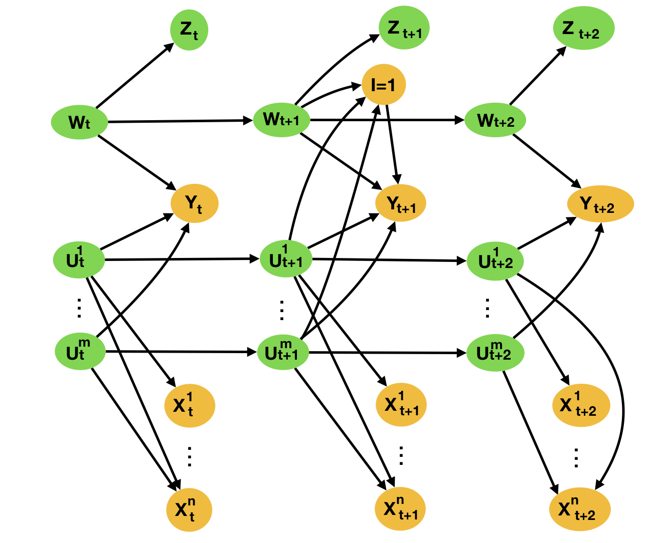
Figure 2: DAG for synthetic control model when there are latent causes of the treated unit that we don’t have observed proxies for. Orange nodes are observed, green nodes are latent.

If there is a latent cause $w^{t}$ with unobserved proxies $z^{t}$, as graphically illustrated in Figure 2, this impacts our identification strategy. In this situation, the updated argument of Theorem 3.1 proceeds as follows. There exists a function $H$ such that $P(y^{t}\mid u^{t},I^{t},w^{t})=\iint H(y^{t},x^{t},z^{t},I^{t})P(x^{t},z^{t}\mid u^{t},I^{t},w^{t})dxdz.$ This implies that:

$$\mathbb{E}\left(y^{t}\mid u^{t},I^{t}\right) =\iiiint y^{t}H(y^{t},x^{t},I^{t},z^{t})P(x^{t},z^{t}\mid u^{t},I^{t},w^{t})P(w^{t})dydxdzdw$$

$$\overset{A}{=}\iiiint y^{t}H(y^{t},x^{t},I^{t},z^{t})P(x^{t}\mid u_{t})P(z^{t}\mid w^{t})P(w^{t})dydxdzdw$$

$$\overset{A}{=}\int{P(x^{t}\mid u^{t})}\int\underbrace{\left[\int{y^{t}H(y^{t},x^{t},I^{t},z^{t})}dy\right]}_{:=g(x^{t},I^{t},z^{t})}P(z_{t})dzdx$$

$$=\int\mathbb{E}_{P(z^{t})}\left(g(x^{t},I^{t},z^{t})\right)P(x^{t}\mid u^{t},I^{t})dx$$

$$=\mathbb{E}\left(\underbrace{\mathbb{E}_{P(z^{t})}\left(g(x^{t},I^{t},w^{t})\right)}_{:=h(x^{t},I^{t},P(z^{t}))}\mid u^{t},I^{t}\right).$$

Where lines A follow as $x^{t},z^{t}$ are independent of $I$, and $w^{t},u^{t}$ respectively. Yielding the Theorem:

Theorem 3.

The introduction of latent $w^{t}$ with no observable proxies, as graphically depicted in Figure 2, changes the estimand in Theorem 3.1 to:

$$\mathbb{E}\left(y^{t}\mid\text{do}(I^{t}=0),I^{t}=1\right)=\mathbb{E}\left(h(x^{t},I^{t}=0,P(z^{t}))\right).$$

Hence our estimation of the counterfactual depends on the distribution $P(z^{t})$. If this distribution is the same for all time periods, our estimation should proceed in an unbiased fashion. However, if there is a distribution shift in $P(z^{t})$ between the pre-intervention period (time points for which $I=0$) and the post-intervention period (time points for which $I=1$) then our estimate for the effect of treatment on the treated could be biased. Why is this? Well when we learn the function $h$, we only have access to pre-intervention data. Hence, if the latent cause—and thus the unobserved proxies—undergo a distribution shift, this can bias our model, as the $h$ we learn depends on the distribution of the proxies at the time at which we learnt it, which is before the intervention was applied. The bias is thus given by:

$$\text{Bias}=\big{|}\mathbb{E}\left(h(x^{t},I^{t}=0,P_{pre}(z^{t}))\right)-\mathbb{E}\left(h(x^{t},I^{t}=0,P_{post}(z^{t}))\right)\big{|}$$ (2)

3.3 Bounding bias in standard linear synthetic control models

When we consider the case where $h$ is a linear function of the proxies—the standard case employed in previous works, see [Abadie et al.(2010)Abadie, Diamond, and Hainmueller]—the bias takes on a simpler form. That is, if the $z^{t}$ are the unobserved proxies of the latent $w^{t}$, as shown in the DAG in Figure 2, then we can write:

$$h(x^{t},I=0,P(z^{t})) =\mathbb{E}_{P(z^{t})}\left(\sum_{i}^{N}\beta_{i}x^{t}_{i}+\sum_{j}^{M}\gamma_{j}z_{j}^{t}\right)=\sum_{i}^{N}\beta_{i}x^{t}_{i}+\sum_{j}^{M}\gamma_{j}\mathbb{E}_{P(z^{t}_{j})}\left(z^{t}_{j}\right)$$

In this case, Theorem 3 implies that the bias can be written as:

Bias $$=\big{|}\mathbb{E}\left(h(x^{t},I=0,P_{pre}(z_{t}))\right)-\mathbb{E}\left(h(x^{t},I=0,P_{post}(z_{t}))\right)\big{|}$$

$$=\bigg{|}\sum_{j}^{M}\gamma_{j}\mathbb{E}_{P_{pre}(z^{t}_{j})}\left(z^{t}_{j}\right)-\sum_{j}^{M}\gamma_{j}\mathbb{E}_{P_{post}(z^{t}_{j})}\left(z^{t}_{j}\right)\bigg{|}$$

$$\leq M\max_{j}(|\gamma_{j}|)\max_{j}\left(|\mathbb{E}_{P_{pre}(z^{t}_{j})}\left(z^{t}_{j}\right)-\mathbb{E}_{P_{post}(z^{t}_{j})}\left(z^{t}_{j}\right)|\right)$$

As this bound on the bias is in terms of latent quantities, an analyst will need to make plausibility judgments in order to devise a bound in terms of observable quantities. Indeed, if an analyst believes they have not missed latent causes as important to our problem as the ones they included proxies for, then we can upper bound the bias in the worst case by taking the maximums in the above bound on the bias to be the maximums in the observed proxies. This then leads to the following upper bound on the bias in terms of observable quantities:

$$\text{Bias}\leq N\times\max_{i}(|\beta_{i}|)\times\max_{i}\left(|\mathbb{E}\left(x^{pre}_{i}\right)-\mathbb{E}\left(x^{post}_{i}\right)|\right)$$ (3)

4 Experiments

We now assess the validity of this bound on a series of synthetic and real world data. Using simulations, we investigate our bound in a valid and invalid setting. Moreover, we test on the California Tobacco Tax and German Reunification data-sets to demonstrate the bound in a real world setting.

4.1 Synthetic Experiments

Our synthetic experiments are constructed such that the unobserved latent $w$ experiences a distribution shift after the intervention, leading to bias as defined in Equation 2. To test validity of our bound in Equation 3, we consider two examples: one where the plausibility bounds are satisfied, illustrated in Figure 3(a), and one where they are violated, illustrated in Figure 3(b). Data generation is outlined in Appendix B. Results and discussion are in the caption of Figure 3.

[ ] [ ]

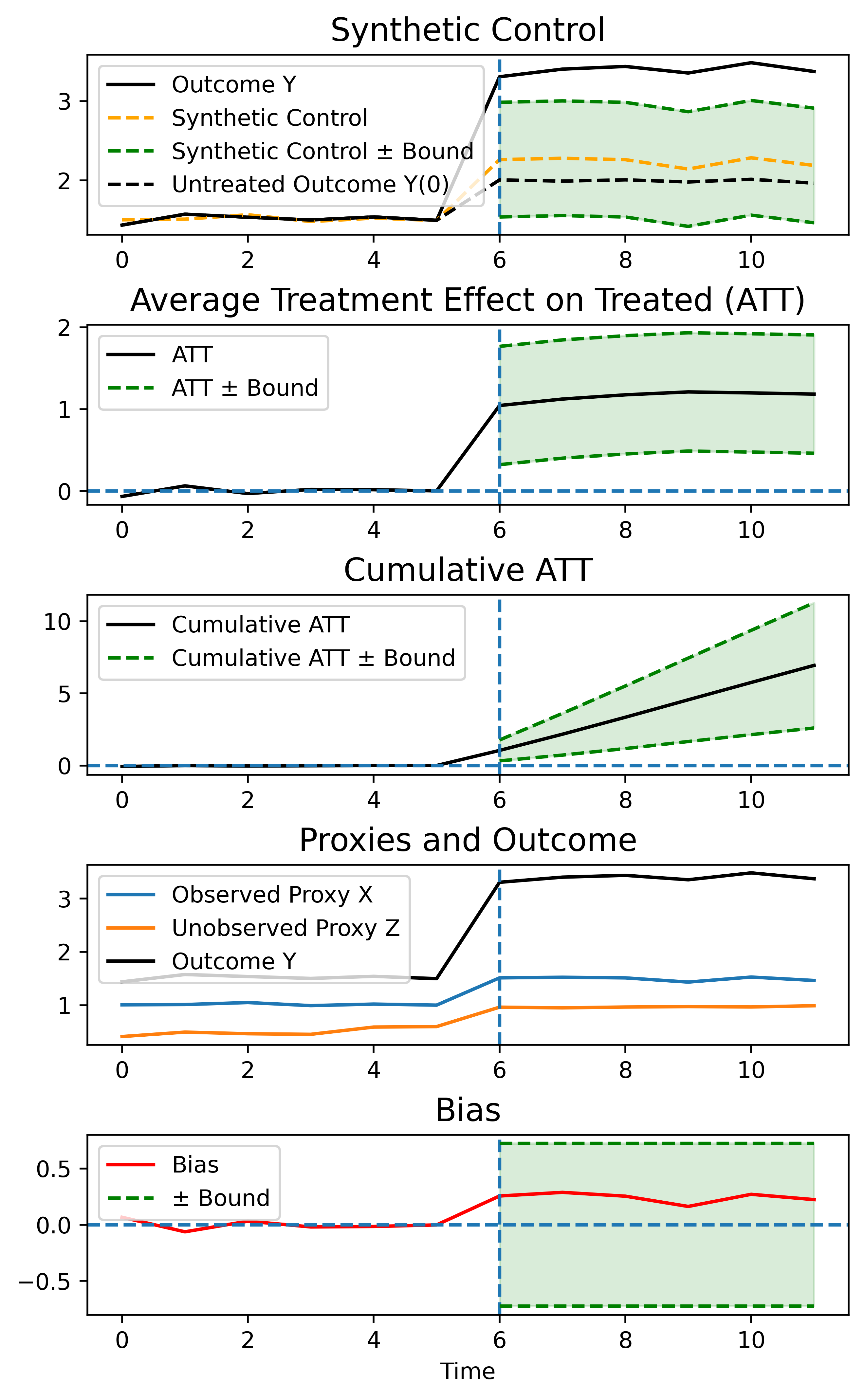
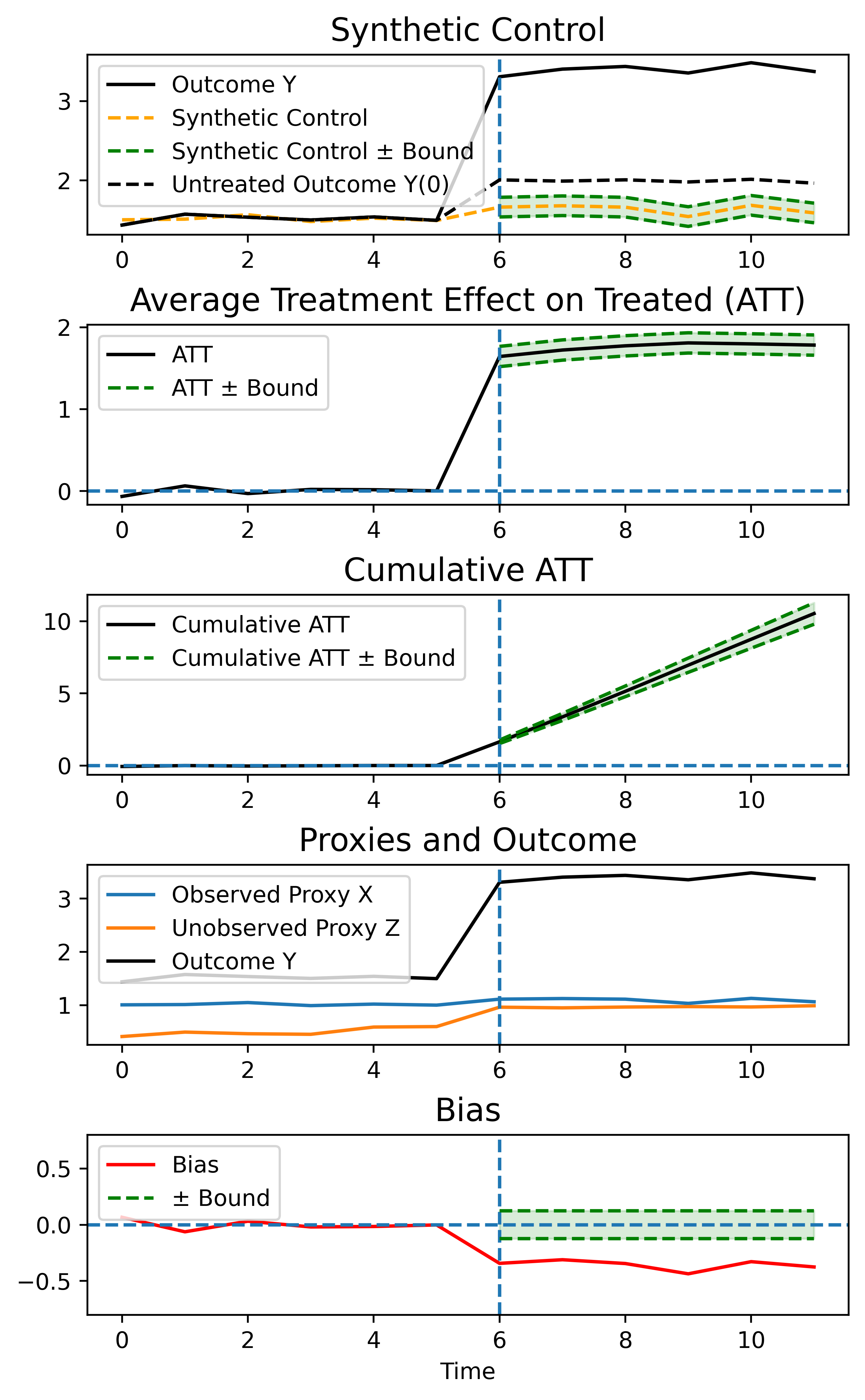
Figure 3: Simulation to evaluate the validity of bound For Scenario (a) we have a valid bound and for Scenario (b) an invalid bound on the bias, i.e. the bounds do not capture the true bias (red, bottom row). The intervention occurs at $T=6$. The first row shows the outcome of interest, as well as its untreated state $Y\mid\text{do}(I=0)$, written as $Y(0)$ in the figure and depicted in black. The synthetic control is shown as a dashed orange line contained by the bounds in green. The second row shows the average treatment effect on the treated (ATT) by subtracting the synthetic control from the observed outcome and averaging. The third row shows the cumulative effect over time. Row four shows the progression of all proxies, observed and unobserved as well as the outcome over time. The last row shows the bias as defined by the true untreated outcome subtracted from the synthetic control. (a): The bias (red) is contained by the bounds. Given the bounds do not contain 0 in the ATT plot, the effect measured is still positive even if we had a worst case bias, given our assumptions. Thus, when our plausibility assumptions are satisfied, so too is our bound on the bias. (b): The observed proxy $X$ shifts less during the intervention time (blue) such that the bound is smaller as we measure a smaller change in the proxies. As a consequence, the bias (red) is outside the bounds. Hence, when our plausibility assumptions are violated, so too is our bound on the bias.

4.2 Real Data

In our first experiment on real data, we look into a tobacco tax increase of 25 cents introduced in California in 1988 [Abadie et al.(2010)Abadie, Diamond, and Hainmueller]. We build a synthetic control to predict the untreated annual per-capita cigarette sales of California, using sales data from the states used in the literature: Colorado, Connecticut, Montana, Nevada, Utah. For our second experiment we refer to the 1990 reunification of West and East Germany in [Abadie et al.(2015)Abadie, Diamond, and Hainmueller]. Here, we build a synthetic control model to predict the untreated GDP of West Germany using GDP data from the countries used in the literature: USA, Austria, Netherlands, Switzerland, Japan. We run a linear regression for each synthetic control, without intercept and allowing for negative coefficients. In line with [Brodersen et al.(2015)Brodersen, Gallusser, Koehler, Remy, Scott, et al.], we calculate the ATT as a running average in $T_{post}$.

[ ] [ ]

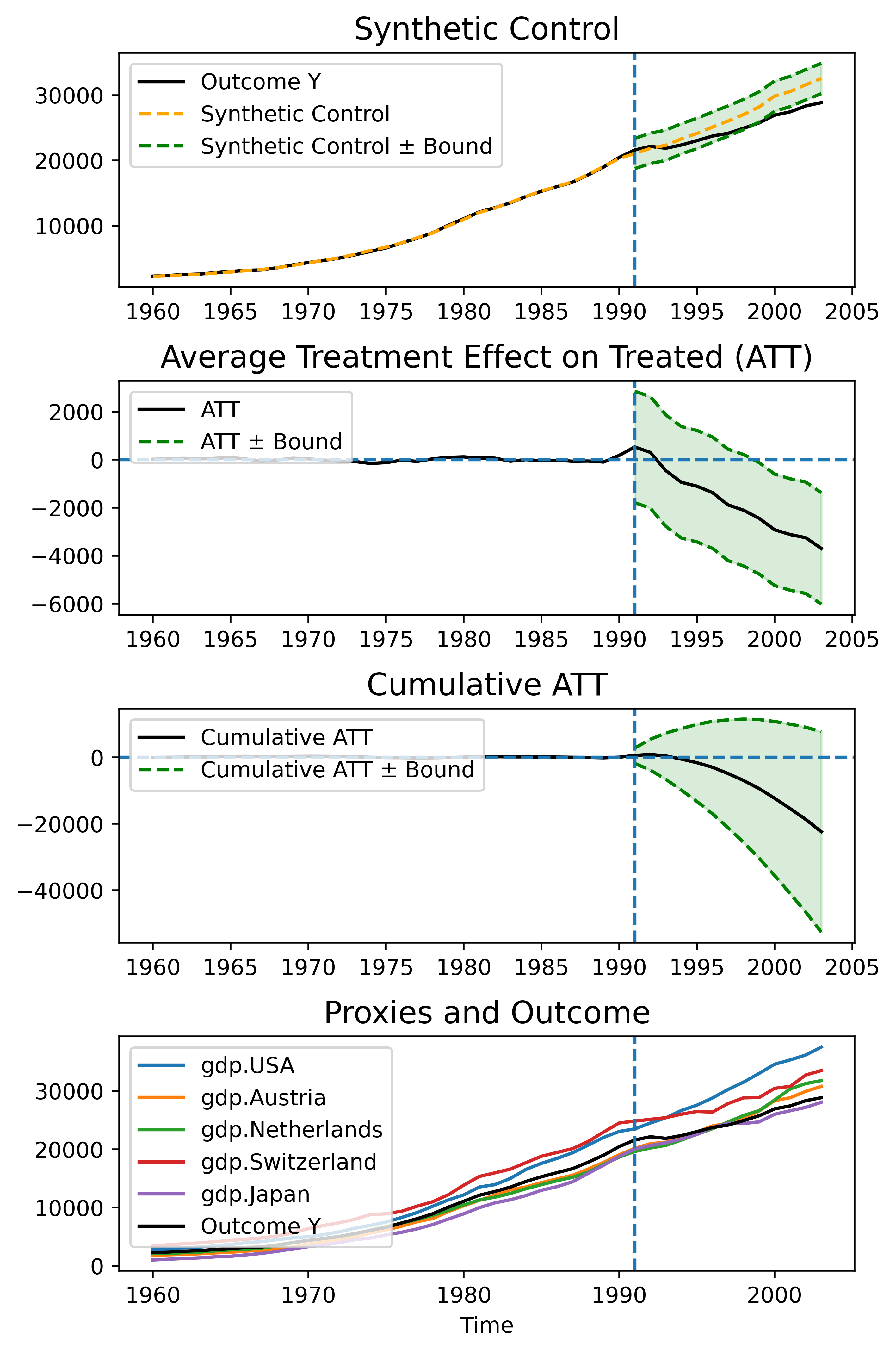
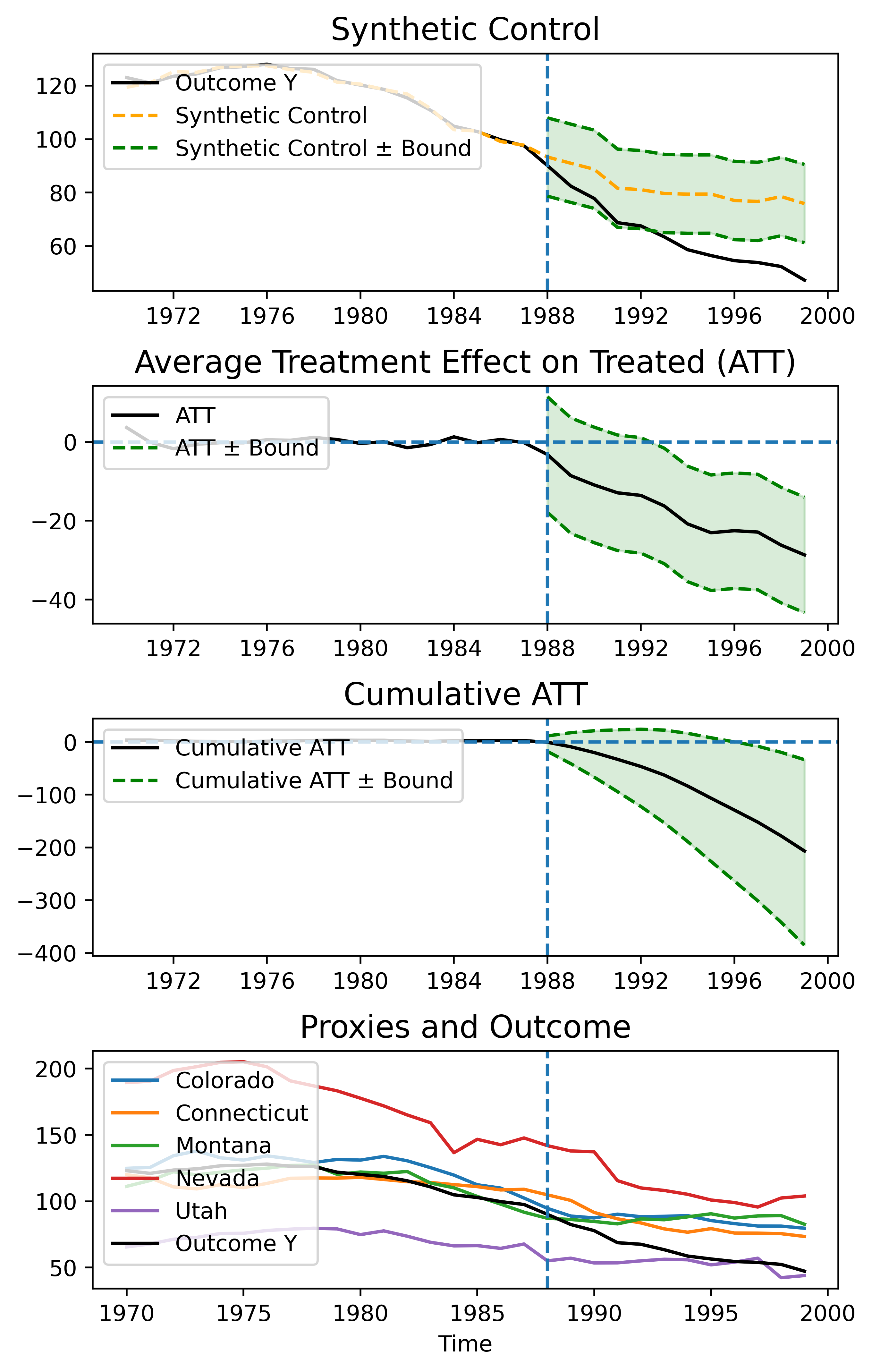
Figure 4: Real World Examples (a): German Reunification: The reunification occurred in 1991 leaving West Germany with a visible drop in its previous growth. Our bound of 2321.84 does not allow to conclude that, given our assumptions, the average ATT is not reversed by other latent variable shifts by $u$. The bound on the bias is primarily driven by the high levels of variation in Switzerland (red, bottom plot) which around the time of the reunification also changed into a phase of slower growth. (b): California Tobacco Tax: Our bound of 14.65 is smaller than the average ATT of -17.45 and allows us to conlcude, that given the assumptions, that even if there was an unobserved bias as big in contribution as the observed proxies, the negative causal effect would persist. Based on that reasoning, the California Tobacco Tax can be deemed as effective in reducing smoking.

Table 1 shows the bounds our method yields. For German Reunification, we have $N=4$ as Japan’s coefficient is zeroed. The biggest beta coefficient corresponds to Austria with 0.46. The proxy change is 1252, yielding a bound of 2321.84. With an average ATT of -1726.8, given our assumptions, this bound on the bias tell us that the causal effect we have estimated is very sensitive. This is, in the worst case, the causal estimate in this case can be entirely due to a shift in an unobserved latent. For California Tobacco, we have $N=4$ as the regression zeroes the coefficient on Utah, leaving 4 proxies. Montana has the biggest regression coefficient with 0.4. The maximum change in the proxies is 9.1, yielding a bound of 14.65, which is smaller than the average ATT of -17.45. In contrast to the German Reunification example, our bound in this example allows us to conclude that—given our assumptions—even with the worst case bias, the tobacco tax will still have a negative causal effect. See Figure 4 for the corresponding synthetic control plots.

Data	N	Max. Beta	Max. Proxy Change	Bound	average ATT
Germany, 1990	4	0.46	1252	$\pm$2321.84.	-1726.80
California, 1981	4	0.4	9.1	$\pm$ 14.65	-17.45

Table 1: Bounds on bias of ATT for the California Tax and German Reunification Example

By design, sensitivity analysis is a subjective method, as it relies on domain expert knowledge to make a judgement on the empirical evidence given. Our method offers a conservative upper bound on the bias, where both the maximum beta and proxy change are empirical, and the domain expert is left with the decision which proxies to incorporate into their analysis. Effectively, this is equivalent to the unobserved parameters commonly introduced to models in classical sensitivity analysis [Imbens(2003)], on which the expert has to make their judgement. Here, our aim was not a final judgement on the real world examples shown, but instead to demonstrate of how to enrich expert discussion with our bound for any synthetic control analysis. Ultimately, it is the expert that has to make plausibility judgements in the scientific discourse, and these bounds are a necessary addition to understand robustness against bias.

5 Conclusion

One of the most widely used causal inference approaches are synthetic control methods. However, in all previous identifiability proofs, it is implicitly assumed that the underlying assumptions are satisfied for all time periods both pre- and post-intervention. This is a strong assumption, as models can only be learned in pre-intervention period. In this paper we addressed this challenge, and proved identifiability without the need for this assumption by showing it follows from the principle of invariant causal mechanisms. Moreover, for the first time, we formulated and studied synthetic control models in Pearl’s structural causal model framework. Importantly, we provided a general framework for sensitivity analysis of synthetic control models to violations of the assumptions underlying non-parametric identifiability. We concluded by providing an empirical demonstration of our sensitivity analysis approach on real-world data.

Appendix A Technical conditions for proofs

The proof of Theorem 3.1 relies on some technical conditions which we now overview. See Appendix C of [Shi et al.(2021b)Shi, Miao, Hu, and Tchetgen Tchetgen] and references therein for further details. In order to prove the existence of the function $H^{t}$, we need the following.

Consider the space of all square-integrable functions $s$, denoted $L^{2}\{F(s)\}$, with respect to a cumulative distribution function $F(s)$. This is a Hilbert space with inner product given by $\langle f,g\rangle=\int f(s)g(s)dF(s)$. Let $K_{x}$ denote the conditional expectation operator $L^{2}\{F(w|x)\}\rightarrow L^{2}\{F(\lambda|x)\}$, with $K_{x}h=E[H(w)|\lambda,x]$ for $H\in L^{2}\{F(w|x)\}$, and let $(\tau_{x,n},\varphi_{x,n},\psi_{x,n})_{n=1}^{\infty}$ denote a singular value decomposition of $K_{x}$. Given the following regularity conditions:

1. $\iint f(w|\lambda,x)f(\lambda|w,x)dwd\lambda<\infty$

2. $\int f^{2}(y|\lambda,x)f(\lambda|x)d\lambda<\infty$

3. $\sum_{n=1}^{\infty}|\langle f(y|\lambda,x),\psi_{x},n\rangle|^{2}<\infty$

Then Picard’s theorem implies the existence of the required function $H^{t}$ in Theorem 3.1.

Appendix B Definitions of Synthetic Experiments

Our synthetic experiments are constructed such that the unobserved latent $w$ experiences a distribution shift after the intervention, leading to bias as defined in Equation 2.

$$\epsilon\sim\mathcal{N}(0,1),u\sim\mathcal{N}(1,1)$$ (4)

$$Y=\begin{cases}au+bw+\epsilon,&\text{in }T_{pre}\text{ , }w\sim Bin(1/2)\\ au+bw+2I+\epsilon,&\text{in }T_{post}\text{ , }w\sim Bin(1)\\ \end{cases}$$ (5)

$$Z=\begin{cases}dw+\epsilon,&\text{in }T_{pre}\text{ , }w\sim Bin(1/2)\\ dw+\epsilon,&\text{in }T_{post}\text{ , }w\sim Bin(1)\\ \end{cases}$$ (6)

$$X=\begin{cases}cu+\epsilon,&\text{in }T_{pre}\text{ , }\epsilon\sim\mathcal{N}(0,1)\\ cu+\epsilon,&\text{in }T_{post}\text{ , }\epsilon\sim\mathcal{N}(0.5,1)\\ \end{cases}$$ (7)

$$I=\begin{cases}0,&\text{in }T_{pre}\\ Bin(sigmoid(u))+\epsilon,&\text{in }T_{post}\\ \end{cases}\\$$ (8)

Given this data generation process, we have:

$$\textbf{ Synthetic Control }\E(Y)=\frac{a}{c}\E(X)+\frac{b}{d}\E(Z),\quad\textbf{True Bias}=|b\{\E_{pre}(w)-\E_{post}(w)\}|,\\$$

$$\textbf{ Proxies Bias }=|\frac{b}{d}\{\E_{pre}(Z)-\E_{post}(Z)\}|,\quad\textbf{Our bound on bias}=|\frac{a}{c}\{\E_{pre}(X)-\E_{post}(X)\}|$$

Following from the above equation for the Synthetic Control $\E(Y)$, our bound on the bias holds if the following conditions hold: (1) $\frac{a}{c}>\frac{b}{d}$, i.e the weighting of the contribution of the mean of the unobserved proxies $Z$ is smaller than of the mean of the observed proxies $X$. (2) The change in the mean of proxies $X$ is bigger than the change in the mean of unobserved proxies $Z$.

Given access to the unobserved $w$ and its proxies $Z$ through this simulation, we can validate the bounds. Setting $(a,b,c,d)=(1,0.5,1,0.5)$, Figure 3 showcases the aforementioned conditions in our synthetic setting under a valid and a invalid bound scenario. For Scenario (a), our maximum mean change in proxies $X$ is 0.48 (not exactly 0.5 due to noise terms), $N$ is 1 and the OLS coefficient is 1.47, such that the $\text{bias}\leq 1\times 1.47\times 0.48=0.71$. As expected, the bias (red) is captured by the bounds as both conditions are fulfilled, see bottom graph of Figure 3 (a).

For Scenario (b), if we change the noise term on X in the post intervention stage to $\epsilon\sim\mathcal{N}(0.1,1)$, causing a violation of the second condition, we have a mean change of 0.08 (not 0.1 due to noise), leading to a $\text{bias}\leq 1\times 1.47\times 0.08=0.12$. Hence, the bounds are smaller, but more importantly also invalid as they do not contain the true bias.

Having chosen a simple example for effective exposition, we would like to emphasize that the validity (and invalidity) of the bounds in these scenarios naturally extend to more complex scenarios with higher number of latents $u$ and proxies $X$.

References

- [Abadie and Gardeazabal(2003)] Alberto Abadie and Javier Gardeazabal. The economic costs of conflict: A case study of the basque country. American economic review, 93(1):113–132, 2003.
- [Abadie et al.(2010)Abadie, Diamond, and Hainmueller] Alberto Abadie, Alexis Diamond, and Jens Hainmueller. Synthetic control methods for comparative case studies: Estimating the effect of california’s tobacco control program. Journal of the American statistical Association, 105(490):493–505, 2010.
- [Abadie et al.(2015)Abadie, Diamond, and Hainmueller] Alberto Abadie, Alexis Diamond, and Jens Hainmueller. Comparative politics and the synthetic control method. American Journal of Political Science, 59(2):495–510, 2015.
- [Brodersen et al.(2015)Brodersen, Gallusser, Koehler, Remy, Scott, et al.] Kay H Brodersen, Fabian Gallusser, Jim Koehler, Nicolas Remy, Steven L Scott, et al. Inferring causal impact using bayesian structural time-series models. Annals of Applied Statistics, 9(1):247–274, 2015.
- [Chevalley et al.(2022)Chevalley, Bunne, Krause, and Bauer] Mathieu Chevalley, Charlotte Bunne, Andreas Krause, and Stefan Bauer. Invariant causal mechanisms through distribution matching. arXiv preprint arXiv:2206.11646, 2022.
- [Cinelli and Hazlett(2020)] Carlos Cinelli and Chad Hazlett. Making sense of sensitivity: Extending omitted variable bias. Journal of the Royal Statistical Society: Series B (Statistical Methodology), 82(1):39–67, 2020.
- [Cinelli et al.(2019)Cinelli, Kumor, Chen, Pearl, and Bareinboim] Carlos Cinelli, Daniel Kumor, Bryant Chen, Judea Pearl, and Elias Bareinboim. Sensitivity analysis of linear structural causal models. In International conference on machine learning, pages 1252–1261. PMLR, 2019.
- [Dhir and Lee(2020)] Anish Dhir and Ciarán M Lee. Integrating overlapping datasets using bivariate causal discovery. In Proceedings of the AAAI Conference on Artificial Intelligence, volume 34, pages 3781–3790, 2020.
- [Gilligan-Lee(2020)] Ciarán Gilligan-Lee. Causing trouble. New Scientist, 246(3279):32–35, 2020.
- [Gilligan-Lee et al.(2022)Gilligan-Lee, Hart, Richens, and Johri] Ciarán M Gilligan-Lee, Christopher Hart, Jonathan Richens, and Saurabh Johri. Leveraging directed causal discovery to detect latent common causes in cause-effect pairs. IEEE Transactions on Neural Networks and Learning Systems, 2022.
- [Graham et al.()Graham, Lee, and Perov] Logan Graham, Ciarán M Lee, and Yura Perov. Copy, paste, infer: a robust analysis of twin networks for counterfactual inference.
- [Guo et al.(2022)Guo, Tóth, Schölkopf, and Huszár] Siyuan Guo, Viktor Tóth, Bernhard Schölkopf, and Ferenc Huszár. Causal de finetti: On the identification of invariant causal structure in exchangeable data. arXiv preprint arXiv:2203.15756, 2022.
- [Imbens et al.(2022)Imbens, Kallus, Mao, and Wang] Guido Imbens, Nathan Kallus, Xiaojie Mao, and Yuhao Wang. Long-term causal inference under persistent confounding via data combination. arXiv preprint arXiv:2202.07234, 2022.
- [Imbens(2003)] Guido W Imbens. Sensitivity to exogeneity assumptions in program evaluation. American Economic Review, 93(2):126–132, 2003.
- [Jeunen et al.(2022)Jeunen, Gilligan-Lee, Mehrotra, and Lalmas] Olivier Jeunen, Ciarán M Gilligan-Lee, Rishabh Mehrotra, and Mounia Lalmas. Disentangling causal effects from sets of interventions in the presence of unobserved confounders. arXiv preprint arXiv:2210.05446, 2022.
- [Kreif et al.(2016)Kreif, Grieve, Hangartner, Turner, Nikolova, and Sutton] Noémi Kreif, Richard Grieve, Dominik Hangartner, Alex James Turner, Silviya Nikolova, and Matt Sutton. Examination of the synthetic control method for evaluating health policies with multiple treated units. Health economics, 25(12):1514–1528, 2016.
- [Kuroki and Pearl(2014)] Manabu Kuroki and Judea Pearl. Measurement bias and effect restoration in causal inference. Biometrika, 101(2):423–437, 2014.
- [Lee and Spekkens(2017)] Ciarán M Lee and Robert W Spekkens. Causal inference via algebraic geometry: feasibility tests for functional causal structures with two binary observed variables. Journal of Causal Inference, 5(2), 2017.
- [Miao et al.(2018)Miao, Geng, and Tchetgen Tchetgen] Wang Miao, Zhi Geng, and Eric J Tchetgen Tchetgen. Identifying causal effects with proxy variables of an unmeasured confounder. Biometrika, 105(4):987–993, 2018.
- [Mitrovic et al.(2020)Mitrovic, McWilliams, Walker, Buesing, and Blundell] Jovana Mitrovic, Brian McWilliams, Jacob Walker, Lars Buesing, and Charles Blundell. Representation learning via invariant causal mechanisms. arXiv preprint arXiv:2010.07922, 2020.
- [Parascandolo et al.(2018)Parascandolo, Kilbertus, Rojas-Carulla, and Schölkopf] Giambattista Parascandolo, Niki Kilbertus, Mateo Rojas-Carulla, and Bernhard Schölkopf. Learning independent causal mechanisms. In International Conference on Machine Learning, pages 4036–4044. PMLR, 2018.
- [Pearl(2009)] Judea Pearl. Causality. Cambridge university press, 2009.
- [Perov et al.(2020)Perov, Graham, Gourgoulias, Richens, Lee, Baker, and Johri] Yura Perov, Logan Graham, Kostis Gourgoulias, Jonathan Richens, Ciaran Lee, Adam Baker, and Saurabh Johri. Multiverse: causal reasoning using importance sampling in probabilistic programming. In Symposium on advances in approximate bayesian inference, pages 1–36. PMLR, 2020.
- [Reynaud et al.(2022)Reynaud, Vlontzos, Dombrowski, Lee, Beqiri, Leeson, and Kainz] Hadrien Reynaud, Athanasios Vlontzos, Mischa Dombrowski, Ciarán Lee, Arian Beqiri, Paul Leeson, and Bernhard Kainz. D’artagnan: Counterfactual video generation. arXiv preprint arXiv:2206.01651, 2022.
- [Richens et al.(2020)Richens, Lee, and Johri] Jonathan G Richens, Ciarán M Lee, and Saurabh Johri. Improving the accuracy of medical diagnosis with causal machine learning. Nature communications, 11(1):1–9, 2020.
- [Rosenbaum and Rubin(1983)] Paul R Rosenbaum and Donald B Rubin. Assessing sensitivity to an unobserved binary covariate in an observational study with binary outcome. Journal of the Royal Statistical Society: Series B (Methodological), 45(2):212–218, 1983.
- [Shi et al.(2022)Shi, Sridhar, Misra, and Blei] Claudia Shi, Dhanya Sridhar, Vishal Misra, and David Blei. On the assumptions of synthetic control methods. In International Conference on Artificial Intelligence and Statistics, pages 7163–7175. PMLR, 2022.
- [Shi et al.(2021a)Shi, Miao, Hu, and Tchetgen] Xu Shi, Wang Miao, Mengtong Hu, and Eric Tchetgen Tchetgen. Theory for identification and inference with synthetic controls: a proximal causal inference framework. arXiv preprint arXiv:2108.13935, 2021a.
- [Shi et al.(2021b)Shi, Miao, Hu, and Tchetgen Tchetgen] Xu Shi, Wang Miao, Mengtong Hu, and Eric Tchetgen Tchetgen. On proximal causal inference with synthetic controls. arXiv e-prints, pages arXiv–2108, 2021b.
- [Shpitser et al.(2021)Shpitser, Wood-Doughty, and Tchetgen] Ilya Shpitser, Zach Wood-Doughty, and Eric J Tchetgen Tchetgen. The proximal id algorithm. arXiv preprint arXiv:2108.06818, 2021.
- [Stegle et al.(2010)Stegle, Janzing, Zhang, Mooij, and Schölkopf] Oliver Stegle, Dominik Janzing, Kun Zhang, Joris M Mooij, and Bernhard Schölkopf. Probabilistic latent variable models for distinguishing between cause and effect. Advances in neural information processing systems, 23, 2010.
- [Tchetgen et al.(2020)Tchetgen, Ying, Cui, Shi, and Miao] Eric J Tchetgen Tchetgen, Andrew Ying, Yifan Cui, Xu Shi, and Wang Miao. An introduction to proximal causal learning. arXiv preprint arXiv:2009.10982, 2020.
- [Veitch and Zaveri(2020)] Victor Veitch and Anisha Zaveri. Sense and sensitivity analysis: Simple post-hoc analysis of bias due to unobserved confounding. Advances in Neural Information Processing Systems, 33:10999–11009, 2020.
- [Vlontzos et al.(2021)Vlontzos, Kainz, and Gilligan-Lee] Athanasios Vlontzos, Bernhard Kainz, and Ciaran M Gilligan-Lee. Estimating the probabilities of causation via deep monotonic twin networks. arXiv preprint arXiv:2109.01904, 2021.
- [Wang et al.(2022)Wang, Yi, Chen, and Zhu] Ruoyu Wang, Mingyang Yi, Zhitang Chen, and Shengyu Zhu. Out-of-distribution generalization with causal invariant transformations. In Proceedings of the IEEE/CVF Conference on Computer Vision and Pattern Recognition, pages 375–385, 2022.
- [Zhang and Bareinboim(2022)] Junzhe Zhang and Elias Bareinboim. Can humans be out of the loop? In Conference on Causal Learning and Reasoning, pages 1010–1025. PMLR, 2022.