The Atacama Cosmology Telescope: Flux Upper Limits from a Targeted Search for Extragalactic Transients

Abstract

We have performed targeted searches of known, extragalactic transient events at millimetre wavelengths using nine seasons (2013–2021) of 98, 150, and 229 GHz Atacama Cosmology Telescope (ACT) observations that mapped ${\sim}40$ per cent of the sky for most of the data volume. We observe at least once 88 gamma-ray bursts (GRBs), 12 tidal disruption events (TDEs) and 203 other transients, including supernovae (SNe). We stack our ACT observations to increase the signal-to-noise ratio of the maps. In all cases but one, we do not detect these transients in the ACT data. The single candidate detection (event AT2019ppm), seen at ${\sim}5\sigma$ significance in our data, appears to be due to active galactic nuclei (AGN) activity in the host galaxy coincident with a transient alert. For each source in our search we provide flux upper limits. For example, the medians for the 98 GHz 95 per cent confidence interval upper limits are $28$, $15$, and $16$ mJy for GRBs, SNe, and TDEs respectively. The sensitivity of future wide-area cosmic microwave background (CMB) surveys should be good enough to detect many of these events using the methods described in this paper.

1 Introduction

For more than a decade, ground-based cosmic microwave background (CMB) telescopes have been scanning large fractions of the sky—about 40 per cent in the case of the Atacama Cosmology Telescope (ACT)—at millimetre (mm) wavelengths with arcminute resolution. The next generation of CMB experiments, such as the Simons Observatory (SO; Ade et al., 2019) and CMB-S4 (Abazajian et al., 2019) will continue to observe large fractions of the sky with regular cadences of a few days and exceptional sensitivity. This is opening up the possibility for mm time domain science, a largely unexplored field. Recently, ACT serendipitously detected three events consistent with nearby stellar flares (Naess et al., 2021a), while a systematic search of the South Pole Telescope (SPT) data detected 12 events that seemed to be stellar flares and two others that may be extragalactic in origin (Guns et al., 2021). Previously, SPT performed a blind search for transients, finding an extragalactic candidate at $2.6\sigma$ significance with a duration of a week (Whitehorn et al., 2016).

Of particular interest are extragalactic transient sources dominated by synchrotron emission from the rapid ejection and interaction of material from jets and outflows, such as gamma-ray bursts (GRBs), tidal disruption events (TDEs) and supernovae (SNe). Their mm fluxes are not well constrained, and yet this region of the spectrum is important for determining the physical conditions and emission mechanisms of these objects. A CMB mm survey instrument like ACT is ideal for following up such events discovered at other wavelengths due its wide coverage and the fact that it returns to a given location of the sky multiple times per week.

Only a handful of mm observations of nearby SNe exist (e.g., Horesh et al., 2013). The best example of an SN-like event that could have been easily observed by a CMB experiment was the Fast Blue Optical Transient (FBOT) AT2018cow (Ho et al., 2019), a bright and rapidly evolving transient that lasted ${\sim}100$ days, with a ${\sim}100$ GHz flux of ${\sim}90$ mJy 22 days after discovery. However, this might be a rare event that happens to be both very bright and nearby (${\sim}60$ Mpc). A relatively nearby supernova, like SN 2011dh, at a distance of only 7.5 Mpc, will have a flux of ${\sim}4$ mJy four days after discovery that decays thereafter (Horesh et al., 2013). Interacting SNe (characterised by their shock interaction with a very dense circumstellar medium (CSM), namely SNe type IIn and Ibn) is an area where a mm detection would prove invaluable. The radio peak of these happens at later times (${\sim}$hundreds of days), when they become detectable. However, they peak in the mm much earlier ($\lesssim 100$ days) when the interaction with the CSM is at higher densities (Bietenholz et al., 2021; Yadlapalli et al., 2022).

TDEs correspond to the destruction of stars by the supermassive black holes at galaxy centres. The accretion disc formed from the star’s material can create radio-loud on-axis relativistic outflows in a few cases. Additionally, off-axis, non-relativistic radio-quiet emission sometimes can be detected in the mm (Alexander et al., 2020). Yuan et al. (2016) found the TDE IGR J12580+0134 in archival Planck data, likely due to non-relativistic emission from an off-axis jet. Cendes et al. (2021) reported Very Large Array (VLA) and Atacama Large Millimeter Array (ALMA) observations of the non-relativistic TDE AT2019dsg. They measure a 100 GHz flux of 0.07 mJy 74 days after discovery with ALMA. The most luminous example of on-axis relativistic emission from a TDE is J164449.3+573451, whose radio emission peaked $\sim 100-200$ days after discovery (Berger et al., 2012). Examples of mm emission from TDEs suggest that they are observable in this range for several months at least. In a similar vein to interacting SNe, jets from TDEs interact with the circumnuclear medium (CNM). Mm observations of TDEs probe the CNM density and magnetic field on sub-parsec scales, and measurements of mm emission would be key for detecting jets at early stages since the emission is optically thinner at longer wavelengths (Yuan et al., 2016).

A GRB occurs when the highly energetic explosion produced by the core collapse of a massive star creates relativistic, highly-collimated jets. As jets penetrate into the surrounding material, a forward shock expands outwards and produces a cascade of longer wavelength emission, known as the GRB afterglow. It can peak on a time scale of ${\sim}10$ days (de Ugarte Postigo et al., 2012), while a reverse shock moves inwards through the jet itself, accelerating electrons and producing synchrotron emission. This reverse shock peaks in the mm range at a much shorter timescale of a few hours (Laskar et al., 2018, 2019), which can be used to probe the physical conditions of the environment. A typical long GRB (LGRB) at $z\sim 1$ ($\sim 6.7$ Gpc) is expected to peak at ${\sim}1{-}2$ mJy a few days after the burst at 100 GHz (Eftekhari et al., 2022).

In this paper, we search for SNe, TDEs, GRBs, and assorted astronomical transients (ATs) discovered at other wavelengths in ACT mm-wave observations between 2013 and 2021. To give a sense of the detection prospects, the ACT 98 GHz frequency band is capable of detecting a 50 mJy point source at $3\sigma$ with a single observation of two detector arrays (see Section 2.1 for the definition of an array).

While ACT lacks the sensitivity to detect the typical mm flux expected from the types of sources we are targeting, there is always the possibility of discovering unexpectedly high emission from an unusual event, such as AT2018cow, and we can also probe to lower fluxes by stacking over longer time spans. Furthermore, it is now opportune to use the many years of ACT data to develop techniques for performing systematic searches for transient events that will further increase the science output of future experiments, like SO and CMB-S4, which will have better sensitivity.

This paper is organised as follows: Section 2 describes the ACT observations and the matched filter method used to measure the flux from the maps. Section 3 describes how we choose the sources to cross reference with the ACT observations. In Section 4, we show our results. Finally, we present our conclusions in Section 5.

For calculating cosmological distances, we assume a flat cosmology with $\Omega_{\rm m}=0.31$ and $H_{0}=67.7$ km s^-1 Mpc^-1, as measured by Planck Data Release 3 (Planck Collaboration et al., 2020).

2 Observations and Methods

2.1 ACT

In this paper, we use observations from the second and third generations of receivers, ACTPol (Niemack et al., 2010; Thornton et al., 2016) and AdvACT (Henderson et al., 2016; Choi et al., 2018), respectively. These used the same cryostat, which houses three optics tubes, each containing an array of transition-edge sensor (TES) bolometers. Arrays were occasionally changed between observing seasons, such that the data analysed in this paper come from six arrays, denominated PA1 through PA6. Together, these cover three bandpasses: f090 (77–112 GHz), f150 (124–172 GHz), and f220 (182–277 GHz). ACTPol began with PA1 (2013–2015) and PA2 (2014–2016), which observed in the f150 band. The dichroic PA3 (2015–2016) array observed at both f090 and f150. AdvACT replaced PA1 with PA4 (2016 onward) which observed both the f150 and f220 bands, and then replaced PA2/3 with PA5 (2017 onward) and PA6 (2017–2019), each of which observed in both the f090 and f150 bands. Table 1 summarises the frequency channel definitions used in this paper, the effective band centre and band width of each channel and array assuming a synchrotron spectrum $S(\nu)\propto\nu^{-0.7}$, consistent with synchrotron-dominated extragalactic sources, and the dates of the data we searched within.

Table 1: Frequency channels and dates of the data included in the search. Note that there are gaps up to $\mathcal{O}$(months) within the time ranges indicated, due to climate conditions, yearly planned maintenance, upgrades, etc.

Channel	Array	Band	Bandwidth	Synchrotron Band	Data Start Date	Data End Date
		Centre (GHz)a	(GHz)b	Centre (GHz)c
f090	PA3	93.3	31.1	93.2	2015 April 21	2016 December 22
	PA5	96.5	19.0	96.5	2017 May 11	2021 June 18
	PA6	95.3	23.1	95.3	2017 May 11	2019 December 19
f150	PA1	145.4	39.6	145.3	2013 September 10	2016 June 12
	PA2	145.9	36.7	145.7	2014 August 23	2016 December 22
	PA3	144.9	27.8	144.7	2015 April 21	2016 December 22
	PA4	148.5	36.7	148.3	2017 May 11	2021 June 18
	PA5	149.3	28.1	149.2	2017 May 11	2021 June 18
	PA6	147.9	31.1	147.8	2017 May 11	2019 December 16
f220	PA4	226.7	66.6	225.0	2017 May 11	2021 June 18
aThe effective frequency is defined as $\nu_{0}=\frac{\int\nu\tau(\nu)d\nu}{\int\tau(\nu)d\nu}$, where $\nu$ is the frequency and $\tau(\nu)$ is the passband of the channel as a function of frequency.
bThe bandwidth is defined as $\int\tau(\nu)d\nu$.
cFor a $\nu^{-0.7}$ spectrum and assuming a point source.

We only use data taken during the night, defined as falling between 23:00 and 11:00 Coordinated Universal Time, since the telescope has consistent and stable beam profiles during these times. We make maps in specific time intervals (detailed in Section 3) using the standard ACT Maximum Likelihood (ML) mapmaker (Aiola et al., 2020) inside a $2\times 2\,\mathrm{deg}^{2}$ stamp centred on the coordinates of the respective transient, using 10 conjugate gradient steps—enough for the map to converge on the small angular scales relevant for compact sources—and with a downsampling factor of two in the datastream to speed up the map-making process.

Our matched filter (see Section 2.2) takes the instrumental beam as input, for which we use an empirically measured beam determined for each combination of detector array and frequency channel, as described in Aiola et al. (2020). To briefly summarise the process, nighttime maps of Uranus are azimuthally averaged to obtain the radial beam profile and the harmonic beam window function. We use the ‘jitter’ beams (Lungu et al., 2022), which include corrections to account for small pointing variations from night to night and are calculated on maps after additional corrections take place due to pointing jitter. They also made the small correction for the different response across each frequency passband to the CMB blackbody spectrum and a Rayleigh-Jeans spectrum expected for Uranus. Finally, we apply a first-order correction to the harmonic transform of the beam $B(\ell)^{\prime}=B(\ell\nu_{\rm CMB}/\nu_{\rm syn})$ (Hasselfield et al., 2013), where $\nu_{\rm CMB}$ is the effective band centre of the channel and array for a CMB blackbody spectrum and $\nu_{\rm syn}$ is the effective band centres for a $S(\nu)\propto\nu^{-0.7}$ synchrotron spectrum listed in Table 1.

2.2 Matched filter

To measure the flux of sources in our maps, we use the matched filter (MF) approach, which maximizes the signal-to-noise ratio (S/N) of point sources by inverse covariance-filtering the beam-deconvolved map. We follow the approach derived in detail in Section 4.3.2 of Naess et al. (2021b); below we summarize the process.

In terms of the standard (non-deconvolved) brightness-temperature map $\bm{m_{\rm T}}$, the flux is given by

$$\bm{\rho}=\bm{\mathrm{B}}\bm{\mathrm{N}}^{-1}\bm{m_{\rm T}}\text{,}$$ (1)

where $\bm{\mathrm{B}}$ is the instrument beam (diagonal in harmonic space) and $\bm{\mathrm{N}}$ is the noise covariance matrix of the map (which for the purpose of point source finding includes not only instrument and atmospheric noise, but also the CMB and other foregrounds/backgrounds). Equation 1 applies in both the real and the harmonic basis. This definition maximizes S/N, while the following normalization factor $\kappa$ is useful to compute the physical units required for the analysis:

$$\bm{\kappa}=\mathrm{diag}(\bm{\mathrm{B}}\bm{\mathrm{N}}^{-1}\bm{\mathrm{B}})\text{.}$$ (2)

With this we can calculate the flux map, $\bm{f}$, its standard deviation, $\Delta\bm{f}$, and the S/N map, $S/N$, as:

$$\bm{f} =\bm{\rho}/\bm{\kappa}, \Delta\bm{f} =\bm{\kappa}^{-\frac{1}{2}}, S/N=\bm{\rho}\bm{\kappa}^{-\frac{1}{2}}\text{.}$$ (3)

Note that $\bm{m_{\rm T}}$, $\bm{\rho}$ and $\bm{\kappa}$ are all vectors in real space (with each element representing a pixel in the map), so the divisions here are done element-wise. ACT maps normally represent the variations, in $\mathrm{\SIUnitSymbolMicro K}$, around the mean CMB blackbody temperature, but we transform them to units of Jy sr^-1, by multiplying by the derivative of the blackbody spectrum $I_{\rm BB}$ with respect to the temperature, $\partial I_{\rm BB}/\partial T\times 10^{-6}$, evaluated at the frequency of the corresponding channel and $T_{\rm CMB}=2.725$$\mathrm{K}$ (Fixsen, 2009). The factor of $10^{-6}$ accounts for the $\mathrm{\SIUnitSymbolMicro K}$ to $\mathrm{K}$ conversion.

As a ground-based microwave telescope, ACT has to look through the spatially and temporally varying water vapour distribution of the atmosphere, whose turbulence acts as a large source of correlated noise. This leads to the map noise covariance matrix being complicated to model. We use the estimate $\bm{\mathrm{N}}^{-1}=\bm{\mathrm{H}}\bm{\mathrm{C}}^{-1}\bm{\mathrm{H}}$, where $\bm{\mathrm{H}}=\bm{\mathrm{W}}^{\frac{1}{2}}$, and $\bm{\mathrm{W}}$ is the inverse variance, a matrix representing an estimate of the white noise inverse variance per pixel, which is available as an output from the mapmaker. We employ the Fourier-diagonal approximation $\bm{\mathrm{C}}^{-1}=1/(1+(\bm{k}/k_{\rm knee})^{-3})$ for the noise correlation properties, with $k_{\rm knee}=2000$ for f090, 3000 for f150, and 4000 for f220. As such, the noise covariance matrix, $\bm{\mathrm{N}}$, contains correlated $1/f$ noise modulated spatially by the inverse covariance $\bm{\mathrm{W}}$. Note that $\bm{\mathrm{B}}$, $\bm{\mathrm{H}}$, $\bm{\mathrm{C}}$, and $\bm{\mathrm{N}}$ are matrices; $\bm{\mathrm{B}}$ and $\bm{\mathrm{C}}$ are harmonic representations and are diagonal in harmonic space (since we treat the beam as azimuthally symmetric), while $\bm{\mathrm{H}}$ is a pixel representation and diagonal in pixel space (we do not compute the correlations among pixels), as well as $\bm{\mathrm{W}}$.

2.3 Astrophysical background

For every matched filter map we produce, we subtract the astrophysical background, which will often include the host galaxy of the transient plus any other background contamination, calculated from depth-1 maps. We consider the potential time window in which a transient source might be active (e.g., from $-$28 to +84 days measured from discovery date for SNe and TDEs; see Section 3), and we calculate the background flux from stacking the depth-1 maps 350 days before and after this time window. With this, we try to achieve a balance between a relatively short time range resolution and having enough data to construct a robust background signal. We use the same matched filter methods, frequency band centres, and beams that we use for the transient maps themselves. We have only produced depth-1 maps from the 2017 season onward; where the depth-1 maps are lacking, we use the Data Release 5 (DR5) coadded ACT maps at the relevant frequency from Naess et al. (2020) (which are coadds of 11 ACT seasons in the period 2008–18) to estimate the astrophysical background. In all cases, we mask bright point sources from the ACT catalogue with flux above 100 mJy to a radius of 3 arcmin.

Since we are subtracting two flux matched filter maps—the short-time scale map, $\bm{f}$, with inverse covariance, $\bm{\kappa}$ (equations 3 and 2, respectively), and the background map, $\bm{f}_{\rm bkg}$, with inverse covariance $\bm{\kappa}_{\rm bkg}$—we need to calculate the inverse covariance of the new map. If $\bm{f}^{\prime}=\bm{f}-\bm{f}_{\rm bkg}$, then $\bm{\kappa}^{\prime}=\bm{\kappa}\bm{\kappa}_{\rm bkg}/(\bm{\kappa}+\bm{\kappa}_{\rm bkg})$.

In some cases, our maps of transient candidates contain only one or a few individual observations, typically because coverage of that part of the sky is poor due to being near the edge of the field of observation. We do not report a flux when its error bar is $>500$ mJy. Furthermore, to account for uncertainty due to variations in the flux calibration from observation to observation, we increase the measured flux error bars using the estimated standard deviation of fractional residual light curves from Uranus observations. For f090, this uncertainty is ${\sim}$1–3 per cent, for f150 it is ${\sim}$2–8 per cent, and for f220 it is ${\sim}$4–12 per cent. Appendix A describes this measurement and procedure in detail.

3 Selection of extragalactic sources

For our targeted extragalactic transient search, we choose GRBs detected with the Neil Gehrels Swift Observatory (Gehrels et al., 2004), SNe and ATs from the comprehensive Open Supernova Catalog (Guillochon et al., 2017), and the TDEs listed in the recent review by Gezari (2021) as well as TDEs recently discovered in X-rays by the SRG All-Sky Survey (Sazonov et al., 2021) at the eROSITA instrument aboard the Spektr-RG space observatory (Predehl et al., 2021; Sunyaev et al., 2021). We consider different time intervals for the different sources we analyse, justified in the subsections that follow below, producing maps containing data from 3 consecutive days, 7 consecutive days (1 week), 28 consecutive days (1 month), 56 consecutive days (2 months), and 84 consecutive days (3 months).

3.1 SNe and ATs

We select transients from the Open Supernova Catalog that compiles SNe discovered from multiple sources and multiple surveys. Since it also includes reported ATs, we include them in this category. Also, a few cases were solar system objects mistaken for SN that are still part of the Open Supernova Catalog. We checked all of the sources we include in our SN/AT catalogue in the Transient Name Server to make sure they are real extragalactic sources and removed the rest. Although there are several thousand sources in the time range of our observations, in reality a SNe must be relatively nearby to be detectable by contemporary mm-wave telescopes. Since FBOT AT2018cow is an example of an uncommon SN-like event that could be detected with a good S/N by mm experiments (Ho et al., 2019; Huang et al., 2019), we use its redshift $z=0.014$ (Perley et al., 2019) as our upper limit for SNe. For the few examples of observed SNe in mm bands, the emission is months in duration, motivating us to produce maps on month-long intervals, starting a month before the discovery date and continuing to the third month after discovery. Additionally, we make two- and three-month maps after the discovery. In total, we make at least one map for 203 distinct SNe/ATs.

3.2 TDEs

There are fewer than 100 discovered TDEs in the literature. We search for those listed in the review by Gezari (2021), which includes all TDEs identified until 2019. We also use the sample of TDEs discovered during 2020 in X-rays by the SRG All Sky Survey made with the eROSITA instrument (Sazonov et al., 2021), although of the 13 in their catalogue, only two are at low enough declination to appear in the ACT survey region. Since we have examples of TDEs lasting for several months, we use the same time intervals for maps that we use for SNe. In total, we make at least one map for 12 distinct TDEs.

3.3 GRBs

GRBs are selected from the database of the Swift observatory. The mission discovers ${\sim}100$ GRBs per year, using the Burst Alert Telescope (BAT), which has a wide field of view and operates in the gamma ray range of 15–150 keV. Within 90 seconds of a trigger from BAT, the satellite is pointed to the approximate position of the source and observes it with the X-Ray Telescope (XRT) and UV/Optical Telescope (UVOT), obtaining precise coordinates for each event. We use the coordinates of the GRB as measured by the XRT, which have a precision of a few arcseconds. The GRB afterglow emission is visible for hours and even several days in the mm range. For this reason, we produce maps of the observations in blocks of three days, starting three days before and up to 15 days after the discovery of the GRB. We also produce maps with seven days of observations, starting seven days before and finishing 28 days after the discovery of the GRB. Finally, we produce a one month map using the 28 days after the discovery day of the GRB. In total, we make at least one map for 88 distinct GRBs.

4 Results

For every time interval before and after the discovery date of a transient specified in Section 3, we produce a map for each detector array and frequency channel that was observing at the time. For each individual map, we estimate the excess flux over the background at the location of the transient candidate with the procedures described in Section 2.2.

For sources with measurements in the same frequency channel and time interval, but from two or more arrays, we calculate the mean flux $\hat{f}$ by weighting each map with its inverse variance at the position of the transient source. That is, $\hat{f}=\sum_{i}f_{i}\Delta f_{i}^{-2}/\sum_{i}\Delta f_{i}^{-2}$ and $\Delta\hat{f}=(\sum_{i}\Delta f_{i}^{-2})^{-1/2}$, where $f_{i}\pm\Delta f_{i}$ is the flux measurement at the transient position for array $i$.

As we do not detect mm counterparts with high confidence for any of the transients in our search, except in the case of AT2019ppm described below, all of our results are upper limits, quoted at the 95 per cent confidence level. We calculate this by integrating the Gaussian probability density function, $p(f)$, which has the mean of the measured flux, $f$, and a standard deviation equivalent to the error bar from the map (equation 3), in order to calculate $f_{95}$, implicitly defined by the equation:

$$\int_{0}^{f_{95}}p(f)df=0.95\int_{0}^{\infty}p(f)df.$$ (4)

Note that we discard the negative portion of the Gaussian distribution.

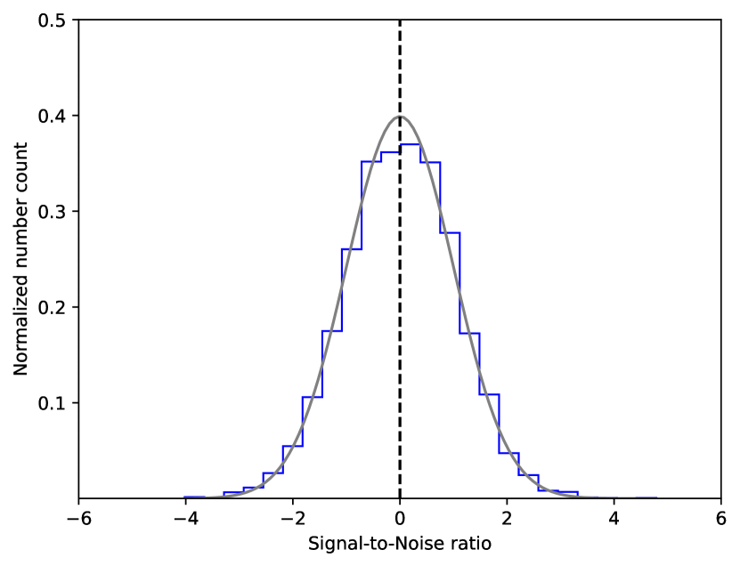
Figure 1: Histogram of the S/N of the flux measurements for all time intervals for all transients types in all frequency channels and all detector arrays. A standard normal probability density function is overplotted in grey.

The histogram of the S/N of our measured flux excess for the candidate transient sources is shown in Figure 1, with a standard normal probability density function overplotted. According to the Anderson-Darling test (e.g., Stephens, 1974) it is consistent with a normal distribution, indicating that the ensemble of our events is consistent with random fluctuations in the map with no evidence for transient detections in the total sample of measurements. The test returns a value of 0.685, which exceeds the critical value for the 10 per cent significance level. We do not consider that this rejects the hypothesis of normality with reasonable confidence. We obtain a similar result if we remove the AT2019ppm event (see below) from the histogram. On the other hand, the D’Agostino and Pearsons’s skewness- and kurtosis-based omnibus test (D’Agostino & Pearson, 1973; D’Agostino et al., 1990) shows little evidence for normality ($p$-value $=4.4\times 10^{-3}$). However, this appears to be due to a few high outliers that we discuss shortly; just removing the single high-S/N AT2019ppm event, for instance, yields much better consistency with normality ($p$-value $=0.035$).

Investigating the higher S/N events in more detail, from our 6669 independent maps, we would expect two to 17 events (inclusive) to have S/N $>3$ with 99 per cent confidence if they are normally distributed. We find 22 maps with S/N $>3$, but inspections of their maps reveal that six of them are due to maps with stripy noise and/or incomplete coverage. They also have high S/N in only one array and frequency, while other arrays that observe the same event simultaneously do not show the same high S/N detection. Discounting these six, the number of S/N $>3$ events is not unexpected; those that remain appear to be due to random noise fluctuations in the map. Furthermore, three of the remaining events correspond to AT2019ppm as seen by simultaneous multiple arrays/frequencies, which we believe is explained by AGN activity in the host galaxy: see Section 4.1. Two events have S/N $>4.5$, which is quite unlikely (0.03 per cent) for our sample size. However, one of these (S/N = 4.8) is from AT2019ppm (see above), while the other (S/N = 4.7) has stripes from correlated noise at the edge of the survey where coverage is not good.

Tables 2, 3, and 4 show 95 per cent upper limits or measured fluxes for a few examples of SNe/ATs, TDEs, and GRBs. The columns show the upper limit in the corresponding time interval (in days, with zero being the discovery date of the event). The blank spaces correspond to time intervals where we do not have observations, or cases of longer time intervals that would be redundant (e.g., a map of the first seven days having the same information as a map of the first three days). The tables for the full list of transients that are investigated in this work are available as supplementary material as machine readable tables. As a reference, the median values for the f090 95 per cent upper limits are 15, 16, and 28 mJy for the measurements for SNe, TDEs, and GRBs, respectively.

4.1 AT2019ppm

While this paper does not target AGNs, one of the sources in our SNe/ATs catalogue seems to be a flare from AGN activity. AT2019ppm was reported on September 7, 2017 (Nordin et al., 2019b). Its position coincides with the galaxy NGC 2110, which is also a known Seyfert II galaxy. The transient processing pipeline that reported the event, AMPEL (Nordin et al., 2019a) at the Zwicky Transient Facility (Graham et al., 2019), flags a discovery when it is associated to a “Known SDSS and/or MILLIQUAS QSO/AGN”.

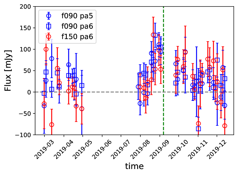
Figure 2: The light curve at the coordinates of the AT2019ppm event is shown using data from ACT’s 2019 observing season in the f090 PA5, f090 PA6, and f150 PA6 channels. We only plot one array for f150 so as not to overcrowd the plot. Each data point corresponds to three days of observations. The dashed green line shows the time when AT2019ppm was reported. These are total flux measurements (i.e., the flux of the background map has not been subtracted). The error bars are $1\sigma$ estimates from the matched filter (equation 3).

All f090 and f150 arrays measure a consistently high signal in the centre of the map in the month before discovery. We measure an excess flux of $49\pm 9$ mJy for f090 and $48\pm 10$ mJy for f150 in this time interval, where we have averaged the fluxes from all arrays at a given frequency; note that this yields a S/N $\approx 5$ for each frequency. The f220 flux does not seem to be significant ($37\pm 35$ mJy, which gives a 95 per cent upper limit of 98 mJy). Light curves for f090 and f150 during ACT’s 2019 season at the AT2019ppm coordinates are shown in Figure 2. The dashed green vertical line shows the discovery time of the transient. Each measurement corresponds to three days of data, and we have only included a single array at f150 so as not to overcrowd the plot. The light curves clearly show rising emission in the month previous to the discovery date. Unfortunately, we have a gap in our observations after the reported date of the AT2019ppm event, presumably during the period where the light curve would have peaked. ACT next observed these coordinates on September 25, 2019, at which point there is no longer any clear excess and when the transient’s flux would presumably have returned to its regular level. Since the AT2019ppm transient is associated with NGC 2110, we conclude that we have detected a flare in the host galaxy’s AGN that lasted for approximately one month. Since the characterisation of the variability of AGNs in the ACT data is a topic of ongoing investigation in the collaboration, we do not further consider them in this work.

Table 2: Examples of the upper limits on flux density for SNe and ATs. The columns correspond to the time range of the map in days, with 0 being the discovery time. The numbers are 95 per cent upper limits and in mJy, except in the case of detections for AT2019ppm. The position is in degrees.

				Time interval for the map relative to alert (in days)
Transient name	RA/Dec	Discovery	Freq.	[$-$28,0]	[0,28]	[28,56]	[56,84]	[0,56]	[0,84]
	deg.			mJy	mJy	mJy	mJy	mJy	mJy
SN2013ft	355.3967/3.7251	2013-09-13	f150	15.2	3.4	2.4	3.5	1.9	1.7
SN2017gax	71.4560/-59.2452	2017-08-14	f090	18.3	19.3	13.4	13.4	12.0	9.6
			f150	7.8	22.2	9.2	16.9	9.1	8.2
			f220	64.1	53.2	54.6	97.8	39.4	38.1
SN2018hdp	33.4377/4.1023	2018-10-08	f090	16.6	8.7	6.4	26.9	4.7	5.3
			f150	18.6	6.6	16.2	22.6	7.1	7.3
			f220	76.0	48.2	54.0	78.6	40.4	35.8
AT2019ppm	88.0475/-7.4564	2019-09-07	f090	$48.6\pm 8.6$	39.6	14.2	15.5	14.6	11.0
			f150	$47.7\pm 9.9$	45.3	22.9	36.6	24.2	24.2
			f220	97.6	167.3	94.3	105.8	83.9	76.0
This table is published in its entirety in the machine-readable format online. A portion is shown here for guidance regarding its form and content.

Table 3: Examples of the upper limits on flux density for TDEs. The columns correspond to the time range of the map in days, with 0 being the discovery time. All measurements are 95 per cent upper limits in mJy. Positions are in degrees.

				Time interval for the map relative to alert (in days)
TDE name	RA/Dec	Discovery	Freq.	[$-$28,0]	[0,28]	[28,56]	[56,84]	[0,56]	[0,84]
	deg.			mJy	mJy	mJy	mJy	mJy	mJy
AT2018fyk	342.5670/-44.8649	2018-09-08	f090	—	10.8	7.9	22.4	5.8	7.4
			f150	—	13.6	11.4	14.6	8.1	6.8
			f220	—	42.4	142.1	32.1	49.3	27.6
AT2019qiz	71.6578/-10.2264	2019-09-24	f090	17.9	14.0	19.4	32.4	13.8	15.1
			f150	19.2	25.5	25.5	19.4	23.3	17.9
			f220	124.7	70.7	96.0	69.7	71.5	49.1
J013204.6+122236	23.0187/12.3766	2020-07-08	f090	28.9	40.3	37.3	16.2	31.4	18.0
			f150	43.4	28.6	16.9	23.6	14.0	12.8
			f220	62.8	72.0	43.8	75.6	36.2	39.8
This table is published in its entirety in the machine-readable format online. A portion is shown here for guidance regarding its form and content.

Table 4: Examples of the upper limits on flux density for GRBs. The columns correspond to the time range of the map in days, with 0 being the discovery time. The numbers are 95 per cent upper limits and in mJy. The position is in degrees.

				Time interval for the map relative to alert (in days)
GRB Name	RA/Dec	Discovery	Freq.	[$-$3,0]	[$-$7,0]	[0,3]	[3,6]	[6,9]	[9,12]	[12,15]	[0,7]	[7,14]	[14,21]	[21,28]	[0,28]
	deg.			mJy	mJy	mJy	mJy	mJy	mJy	mJy	mJy	mJy	mJy	mJy	mJy
131031A	29.6102/-1.5788	2013-10-31	f150	9.9	13.0	23.2	14.3	19.2	10.8	6.7	14.7	8.3	5.3	5.1	4.1
150710A	194.4705/14.3181	2015-07-10	f090	65.3	37.9	115.7	—	33.2	24.8	65.3	46.2	19.5	36.3	19.0	17.7
			f150	29.9	21.9	47.8	—	26.3	46.0	29.9	22.9	26.6	38.1	30.1	17.6
171027A	61.6907/-2.6221	2017-10-27	f090	—	21.8	33.2	18.5	—	23.8	—	14.4	25.8	14.5	13.9	6.5
			f150	—	54.2	28.5	30.6	—	17.0	—	20.5	37.0	16.7	22.7	11.2
			f220	—	295.7	139.5	118.7	—	134.2	—	123.8	148.6	62.8	85.7	61.4
191004B	49.2042/-39.6348	2019-10-04	f090	19.0	28.9	45.0	19.0	41.3	18.5	11.8	16.1	15.9	15.2	46.6	9.8
			f150	31.0	60.8	22.5	28.7	48.6	23.6	22.4	22.6	20.9	41.5	24.2	16.7
			f220	129.6	113.6	140.2	—	181.9	—	93.8	68.0	181.9	94.7	100.3	46.4
This table is published in its entirety in the machine-readable format online. A portion is shown here for guidance regarding its form and content.

4.2 Stacking maps of all sources

To increase the S/N of a potential detection, we stack multiple events together, in the same time intervals and at the same frequencies, for a common class of transient. We use a maximum likelihood approach for the stacking that accounts for the expected S/N of each transient source. Since we do not know the exact measured signal (this is what we are trying to measure in the first place), we use a model-based proxy to estimate it. For each individual map $i$ that is included in the stack, we take its weight to be a ratio of mm fluxes, $R_{i}(\nu_{j},t_{k})$, between the mm flux of transient $i$ (measured at frequency $\nu_{j}$ and time $t_{k}$ after the discovery date), and the mm flux of a reference object, that will be chosen appropriately. Given these weights—how they are estimated and which proxies we use are described further below—we model the measured flux in our maps $\bm{f}_{i}$ (equation 3) as:

$$\bm{f}_{i}=\bm{a}R_{i}(\nu_{j},t_{k})+\bm{n}_{i}\text{,}$$ (5)

where $\bm{n}_{i}$ is the noise of the flux map $\bm{f}_{i}$ with inverse noise covariance $\bm{\kappa}_{i}$ (Equation 2), and $\bm{a}$ is the detection statistic we are optimizing for. Note that a single transient can have multiple maps $\bm{f}_{i}$ if it is observed by multiple detector arrays. The ML solution for $\hat{\bm{a}}$ is:

$$\hat{\bm{a}}=\frac{\sum_{i}R_{i}(\nu_{j},t_{k})\bm{\kappa}_{i}\bm{f}_{i}}{\sum_{i}R_{i}(\nu_{j},t_{k})^{2}\bm{\kappa}_{i}}\text{,}$$ (6)

with a noise inverse covariance $\bm{A}$ given by

$$\bm{A}=\sum_{i}R_{i}(\nu_{j},t_{k})^{2}\bm{\kappa}_{i}\text{.}$$ (7)

The stacked flux at frequency channel $j$ and time interval $k$ is given by the value of $\hat{\bm{a}}$ evaluated at the centre of the map, with uncertainty given by the centre of map $\bm{A}^{-1/2}$. For a given frequency and class of transient, we stack all maps from all detector arrays at the same time interval after the discovery date. Therefore, each of these stacked maps have the same $\nu_{j}$ and $t_{k}$ in their weights. However, to increase the S/N even further, we also stack across frequency channels, across time intervals, and across both. In this case, the weights $R_{i}$ will have varying $t_{k}$ (when stacking across time intervals) and/or varying $\nu_{j}$ (when stacking across frequencies). Thus, for instance, maps from a longer time after the discovery date might have a different weight because of the fading light curve. This is our general stacking procedure, although in practice we only implement it in this fashion for GRBs (see below).

We now turn to how we estimate the weights $R_{i}(\nu_{j},t_{k})$. Ideally, the measured mm flux of each source could be determined by a well-known property, e.g., redshift. However, it is not obvious for any of our transient classes which property (or properties) are the most correlated with their mm fluxes and whether they suffer from selection biases. Additionally, an unbiased reference light curve and spectral energy distribution (SED) must be chosen to shift the $R_{i}(\nu_{j},t_{k})$ to the different frequencies and time intervals. In the following subsections we describe how we address this issue for each class of transient.

4.2.1 SNe Flux Ratios

For SNe, using the flux measured at a wavelength other than the mm is one possible choice, but the optical (and shorter) wavelength emission depends on the explosion itself, while the mm emission is caused by interactions of the SN with the dense, surrounding medium. Instead, we use the distance to the SN given by its measured redshift, which probably has less selection bias. Thus, for SNe we compute $R_{i}(\nu_{j},t_{k})=(D_{\rm ref}/D_{i})^{2}$, where $D_{\rm ref}=7.5$ Mpc, is the distance to our reference, SN 2011dh. Because we use solely the distance squared to estimate the weight, there is no dependence on $\nu_{j}$ or $t_{k}$, so when stacking across frequencies and time intervals, the same transient will receive equal weights, i.e. there is no need to transform to different frequencies or time intervals with a model SED for the reference.

Our choice of SN 2011dh for the reference is motivated by the fact that radio/mm emission from core collapse SNe probably depends on the progenitor and the interaction of the blast wave with the surrounding medium, and positive mm observations have been made of this type of SNe. On the other hand, thermonuclear type Ia SNe happen through a different process which is not expected to generate significant mm emission, and, to date, no mm detection has been made (e.g., Chomiuk et al., 2016; Lundqvist et al., 2020). Thus, we only consider spectroscopically-classified SNe of known types and perform two separate stacks: one for type Ia (55 sources) and one for core collapse SNe (94 sources). Since we use distance squared as our proxy for mm emission, in principle we could do the stack without any reference at all and at any arbitrary distance. However, it is useful to have an emission to compare to. SN 2011dh is a stripped-envelope type IIb SN that is close ($z=0.00168$; Strotjohann et al. 2015), and therefore less prone to selection bias; it also has a measured mm emission (Horesh et al., 2013). Furthermore, although our stacking weights $R_{i}$ are independent of time or frequency, we use the SED model in equations 5 and 6 of the latter paper to estimate an expected flux for any given frequency and time for comparison of our stack results (see Sec. 4.2.4, below).

4.2.2 TDE Flux Ratios

TDEs suffer from a similar complication as SNe, since the radio and mm synchrotron emission depends chiefly on the properties of the circumstellar and interstellar media and on outflows/jets, whereas optical and X-ray emission is often dominated by other processes (Roth et al., 2020). Therefore, we take the same approach as SNe and use the distance squared determined from measured redshifts as our mm flux proxy: $R_{i}=(D_{\rm ref}/D_{i})^{2}$, where $D_{\rm ref}=92.6$ Mpc, the distance to our reference, TDE ASASSN-14li. As with the SNe, the weights have no time/frequency dependence. This source is one of the few available choices we have, but is also one of the best studied examples of off-axis TDEs in radio/mm emission. It is nearby ($z=0.02058$) and has been modelled by several authors (e.g., Alexander et al., 2016; Krolik et al., 2016). For comparison of our stacked fluxes to a fiducial flux (see Sec. 4.2.4, below), we use the SED model shown in Figure 1 and Table 2 of Alexander et al. (2016). Although this paper does not have observations near the ACT frequencies, they are well above the frequency break between optically thick and thin synchrotron emission, and it is safe to assume that the power law that fits observations well at higher frequencies, $S_{\nu}\propto\nu^{-1}$, is valid in our frequency regime.

4.2.3 GRB Flux Ratios

Just like we do in the case of SNe and TDEs, distance squared might be an unbiased estimator of GRB mm flux, but we lack redshift measurements for most of our sample. The mean, 24-hour X-ray flux measured with the XRT aboard Swift seems like a good alternative, since the peak mm flux appears to be correlated with the 10 keV X-ray flux after 12 hours, albeit with significant scatter (see Figure 11 of de Ugarte Postigo et al., 2012). Thus, for GRBs, we use $R_{i}(\nu_{j},t_{k})=B_{i}/B_{\rm ref}$, where $B_{i}$ is the 24-hour X-ray flux measured in erg cm^-2 s^-1, and $B_{\rm ref}=3.33\times 10^{-11}$ erg cm^-2 s^-1 is the X-ray flux of our reference, GRB 130427A. When stacking across frequencies, time, or both, we multiply $R_{i}(\nu_{j},t_{k})$ by $S(\nu_{j},t_{k})/S(95\,{\rm GHz},t=0)$ to normalise to a reference flux at 95 GHz and time $t=0$, where $S(\nu,t)$ is the SED model of GRB 130427A, and the reference time $t=0$ corresponds to the mean flux in the first 3-day interval between 0 and 3 days after discovery. This source is bright, is likely relatively close ($z\approx 0.34$; Levan et al. 2013) and well studied. It seems that there is nothing particularly exceptional about this GRB, other than being close to us (Perley et al., 2014), and therefore it is a good candidate for a representative GRB.

For the SED varying in time, $S(\nu,t)$, we use a standard fireball model (Sari, 1998) for the GRB afterglow, as fitted in Laskar et al. (2013) and van der Horst et al. (2014) for the time dependence, and the model shown in Figure 2 of van der Horst et al. (2014) for the frequency dependence. When stacking across time intervals, we assign a weight of $R_{i}=0$ for maps with negative time intervals (i.e., before the discovery date) since we expect negligible emission before the trigger. For the stacked map across frequencies but at a fixed negative time interval, we use $S(\nu_{j},t=0.5\,{\rm days})$.

4.2.4 Stacking Results

We transform the fluxes of our stacked maps into mm characteristic luminosity $\nu L_{\nu}$, which is more meaningful physically as it does not depend on distance to the source. For both type Ia and core collapse SNe, as well as TDEs, our stacked map are normalised to the flux of a “virtual” reference source either at 7.5 Mpc (in the case of SNe) or 92.6 Mpc (in the case of TDEs), so we can easily assume spherically isotropic emission to transform the measured flux into mm luminosity (including the effect of cosmological redshift). For GRBs, the flux units of our maps are normalised to a GRB with a 24-hour X-ray flux of $3.33\times 10^{-11}$ erg cm^-2 s^-1 (i.e., GRB 130427A). Under the assumption that the population of GRBs we stack are copies of GRB 130427A, then we can assume that our stack map reflects the measured flux of this reference, which is located at a distance of 1852 Mpc. We these caveats we can transform the flux into a mm characteristic luminosity.

The measured characteristic luminosity of the stacked maps are listed in Tables 5, 6, 7, and 8 for core collapse SNe, type Ia SNe, TDEs, and GRBs, respectively. In the tables, the rightmost column shows the maps stacked across time intervals, the bottom row shows the maps stacked across frequency channels, and the bottom right corner shows the overall stack for all time intervals and frequencies. In all tables, except Table 6, we show a reference for the respective frequency and time interval, calculated using the SED model of the reference, as described above. This reference flux is also transformed into characteristic luminosity by using the distance to the reference source.

All of the measurements in the stacked maps show non-detections with small S/N. We conclude that our stacked maps do not contain evidence of any source detection.

Table 5: Characteristic luminosity for stacked core collapse SNe. The units are $10^{3}$ $L_{\sun}$. These results were normalised by a “virtual” reference SN at a distance of 7.5 Mpc. Hence, when transforming flux to characteristic luminosity, it is distance independent. The stacks use all arrays with the same frequency in a given time interval. The rightmost column shows the stacking across time intervals. The bottom row shows the stacking across frequency channels. The bottom right corner shows the stacking across both. The reference shown here is not the same as the one listed in Table 8 for GRBs, but rather it is the characteristic luminosity read from the SED model of SN 2011dh (at a distance of 7.5 Mpc) at the same frequencies and time intervals. We only list them here as a comparison.

Band	days [$-$28,0]		days [0,28]			days [28,56]			days [56,84]			across time
	$\nu L_{\nu}$	err	$\nu L_{\nu}$	err	ref	$\nu L_{\nu}$	err	ref	$\nu L_{\nu}$	err	ref	$\nu L_{\nu}$	err
f090	-0.2	15.3	5.3	12.9	3.0	-13.7	11.1	0.7	18.6	16.7	0.4	-0.6	6.8
f150	-51.0	26.2	-7.3	21.4	3.1	-0.9	19.2	0.7	-18.7	27.5	0.4	-15.3	11.4
f220	349.7	154.7	8.5	141.1	3.5	-4.4	110.8	0.7	47.0	155.7	0.4	77.4	68.2
Across freqs.	-24.2	26.5	1.7	22.1	—	-18.1	19.3	—	11.2	28.3	—	-8.9	11.6

Table 6: Characteristic luminosity for stacked type Ia SNe. The units are $10^{3}$ $L_{\sun}$. These results were normalised by a “virtual” reference SN at a distance of 7.5 Mpc. Hence, when transforming flux to characteristic luminosity, it is distance independent.

Band	days [$-$28,0]		days [0,28]		days [28,56]		days [56,84]		across time
	$\nu L_{\nu}$	err	$\nu L_{\nu}$	err	$\nu L_{\nu}$	err	$\nu L_{\nu}$	err	$\nu L_{\nu}$	err
f090	-10.4	20.0	-10.9	22.1	15.7	25.4	-15.5	29.0	-5.8	11.7
f150	-5.0	32.5	17.0	34.4	30.2	38.0	-60.0	40.9	-1.8	18.0
f220	332.6	178.0	-269.5	208.4	219.4	201.1	-32.3	277.8	100.8	104.1
Across freqs.	-4.1	33.7	-8.4	36.6	49.2	40.9	-65.9	45.6	-4.5	19.2

Table 7: Characteristic luminosity for stacked TDEs. The units are $10^{6}$ $L_{\sun}$. These results were normalised by a “virtual” reference TDE at a distance of 92.6 Mpc. Hence, when transforming flux to characteristic luminosity, it is distance independent. The reference shown here is not the same as the one listed in Table 8 for GRBs, but rather it is the characteristic luminosity read from the SED model of ASASSN-14li (at a distance of 92.6 Mpc) at the same frequencies and time intervals. We only list them here as a comparison.

Band	days [$-$28,0]		days [0,28]			days [28,56]			days [56,84]			across time
	$\nu L_{\nu}$	err	$\nu L_{\nu}$	err	ref	$\nu L_{\nu}$	err	ref	$\nu L_{\nu}$	err	ref	$\nu L_{\nu}$	err
f090	$-1.66$	1.10	$-1.31$	0.86	0.33	0.82	0.62	0.04	1.91	0.77	0.03	0.33	0.39
f150	$-3.10$	1.75	$-0.35$	1.10	0.33	1.11	1.04	0.04	$-0.07$	1.34	0.03	$-0.12$	0.62
f220	12.77	10.04	1.83	7.85	0.33	12.96	6.25	0.04	$-1.68$	6.89	0.03	6.22	3.71
Across freqs.	$-3.76$	1.83	$-1.50$	1.28	—	2.15	1.06	—	2.32	1.34	—	0.50	0.65

Table 8: Characteristic luminosity for stacked GRBs. The units are $10^{9}$ $L_{\sun}$. This is calculated from the mean mm flux for the reference GRB 130427A as explained in Section 4.2.4. We stress that when weighting the stacks and averaging across time and frequency, we make the explicit assumption that every GRB in the stack is a copy of GRB 130427A, scaled by a factor. Under this assumption, the stacked map would have the mean mm flux of GRB 130427A, which is located at a distance of 1852 Mpc. We also show the characteristic luminosity for the reference in each stacked map, where the flux is scaled from the model SED.

Band	days [$-$7,0]		days [$-$3,0]		days [0,3]			days [3,6]			days [6,9]
	$\nu L_{\nu}$	err	$\nu L_{\nu}$	err	$\nu L_{\nu}$	err	ref	$\nu L_{\nu}$	err	ref	$\nu L_{\nu}$	err	ref
f090	3.20	1.92	5.89	2.54	3.56	3.34	0.14	1.75	4.51	0.05	5.35	9.40	0.04
f150	$-5.37$	3.45	$-3.86$	4.83	$-3.53$	6.97	0.19	0.39	8.44	0.07	$-0.24$	14.98	0.06
f220	21.52	20.53	$-1.11$	22.34	18.57	51.57	0.26	57.79	85.87	0.12	170.91	87.41	0.11
Across freqs.	2.24	3.71	6.94	4.87	1.86	2.81	0.14	1.35	3.44	0.05	4.91	6.36	0.04

days [9,12]			days [12,15]			days [14,21]			days [21,28]			across time
$\nu L_{\nu}$	err	ref	$\nu L_{\nu}$	err	ref	$\nu L_{\nu}$	err	ref	$\nu L_{\nu}$	err	ref	$\nu L_{\nu}$	err	ref
1.21	2.47	0.04	-3.87	3.10	0.04	4.15	2.68	0.03	-3.03	2.80	0.02	4.69	1.90	0.14
$-1.25$	4.33	0.06	$-4.57$	4.97	0.06	$-6.27$	4.68	0.04	1.85	4.86	0.03	$-4.65$	3.57	0.19
12.88	26.47	0.10	28.89	31.37	0.07	17.14	29.03	0.05	$-3.34$	28.10	0.04	13.22	18.87	0.26
0.41	1.74	0.04	$-3.03$	2.18	0.04	1.01	2.11	0.03	$-1.41$	2.21	0.02	0.47	0.47	0.14

5 Discussion and conclusions

We have presented a search for excess flux in ACT data before and after the discovery date of 203 SNe and ATs, 12 TDEs, and 88 GRBs. We made no significant detection of excess flux (S/N $<4$ for almost all cases; see Figure 1), except for a single source, AT2019ppm, that seems to be explained by AGN activity of the host galaxy (Section 4.1). We place upper limits for all time intervals considered before and after the transients included in our search at the f090, f150, and f220 ACT frequency channels; the full results are available as supplementary material.

We increased the S/N by stacking maps of multiple sources of the same class, with stacking weights based on educated guesses about how bright the respective source should be in mm emission, but still do not achieve a significant enough S/N for any detection. For core collapse SNe (Table 5), we constrain our stack to have [f090/f150/f220] characteristic luminosity less than [29/38/282] $\times 10^{3}$ $L_{\sun}$ (at 95 per cent confidence level) when measured in the first 28 days of its discovery. As a comparison, SN 2011dh had a characteristic luminosity of [2.4/2.5/2.8] $\times 10^{3}$ $L_{\sun}$ averaged over the first 28 days since its detection for the same 3 ACT frequency channels. For type Ia SNe (Table 6), we constrain our stack to have [f090/f150/f220] characteristic luminosity less than [37/80/269] $\times 10^{3}$ $L_{\sun}$ (at 95 per cent confidence level) when measured in the first 28 days of its discovery. However, this class of SN is not expected to have any detectable mm emission. For TDEs (Table 7), we constrain our stack to have [f090/f150/f220] characteristic luminosity less than [1.1/2.0/16.7] $\times 10^{6}$ $L_{\sun}$ (at 95 per cent confidence level) when measured in the first 28 days of its discovery. As a comparison, TDE ASASSN-14li had a characteristic luminosity of 0.33 $\times 10^{6}$ $L_{\sun}$ averaged over the first 28 days since its detection for all three ACT frequency channels. For GRBs (Table 8), the stack represents the averaged flux as compared to our reference GRB 130427A. That is, assuming that all GRBs have the same intrinsic light curve as the reference, we scaled the ACT flux of a given GRB by the ratio of the reported X-ray flux to the reference flux, and then used the measured distance to the reference to convert to a characteristic luminosity (see Sec. 4.2.3). Under these assumptions, we constrain our stack to have [f090/f150/f220] characteristic luminosity less than [9.5/11.7/114.2] $\times 10^{9}$ $L_{\sun}$ (at 95 per cent confidence level) when measured in the first three days of its discovery. As a comparison, the reference GRB 130427A had a characteristic luminosity of [0.14/0.19/0.26] $\times 10^{9}$ $L_{\sun}$ averaged over the first 3 days since its detection for the same 3 ACT frequency channels. Even when stacking across all frequencies and time intervals, the stacked characteristic luminosity error bar is more than three times larger than the reference characteristic luminosity (S/N $\sim 1/3$).

In conclusion, our non-detection of any extragalactic transient sources is not unexpected, given that ACT does not have the $\lesssim 1$ mJy sensitivity that would be required for most candidates. Extraordinarily rare, very energetic events such as AT2018cow could have been detected at high significance by ACT; as for AT2018cow itself, it was located just north of our survey’s maximum declination and also occurred at a time when the telescope was idle. Future experiments will have the capability of potentially detecting hundreds of on-axis long GRBs (LGRBs) in addition to tens of other events such as FBOTs and on-axis TDEs (Eftekhari et al., 2022). This current paper, however, represents an early effort in the new field of time domain science using mm survey data and introduces methodologies that should be useful for future transient searches. For example, SO’s large aperture telescope (LAT) will have about 4.7 times the number of detectors as ACT did in the f090, f150 and f220 bands when PA4–6 were all installed, corresponding to a ${\sim}2.2\times$ increase in sensitivity to transient events if all frequencies are equally weighted. Furthermore, over its five year campaign, we expect SO to spend roughly a factor of three times longer covering the same ${\sim}40$ per cent of the sky than was analysed in this paper, for a further ${\sim}1.75\times$ increase in sensitivity. Thus, if we stacked regular GRBs in the same fashion we do in this work across frequencies and time intervals, we could potentially increase from S/N $\sim 1/3$ (see Table 8) to S/N $\sim 1.3$. Additional improvements in sensitivity would come with the inclusion of the SO LAT’s 27, 39 and 280 GHz channels (Zhu et al., 2021).

While the targets in our study were known, archival transients, the ACT collaboration is preparing several other time domain projects. We are performing a systematic, optimised blind transient search in which we expect to find tens of new candidates similar to the those discovered serendipitously by Naess et al. (2021a), and another study characterising the variability of AGN is underway. As CMB telescopes continue to deliver impressive cosmological results in the coming years, we can also look forward to a new era of time domain science thanks to their wide-area, high-sensitivity, and short-cadence observations.

Data Availability

The upper limit flux measurements for SNe/ATs, TDEs, and GRBs will be available as machine readable tables on the NASA Legacy Archive Microwave Background Data Analysis (LAMBDA) website. 

Appendix A Estimation of the calibration variance

A key issue in time domain analyses with ACT or any future experiment is characterising how much the calibration changes with time. For ACT, temporal changes in calibration could be caused by variations in the telescope optics, thermal fluctuations in the detector arrays and changes in atmospheric loading and emission, to name a few. The calibration stability can be estimated using an object whose time dependent flux is sufficiently well known a priori, since any deviations from the known flux can be attributed to calibration errors.

We use observations of Uranus to estimate our calibration variance. Uranus was frequently observed throughout the ACTPol and AdvACT data-taking seasons, and is bright enough to provide high SNR in a single observation but not so bright so as to create a non-linear detector response. In addition to Uranus, we considered using the light curves of objects expected to have a constant intrinsic flux, including the brightest dusty point sources identified in the f220 coadded ACT map (Naess et al., 2020), the core of the Orion nebula, the core of the M87 galaxy, and the extended radio lobes of galaxies with AGNs and jets. Each these sources turned out to be more difficult to use than Uranus, either because they have small SNR or are extended and tricky to model as point-like sources. We therefore defer characterising the ACT calibration with these and other sources to a future study.

ACT makes targeted observations of Uranus every few days as part of its routine calibration program, which uses a model of the planet’s brightness to convert power incident on the detectors to brightness temperature units (pW to $\mathrm{\SIUnitSymbolMicro K}$; Aiola et al. 2020). In addition to these targeted observations we used any chance observations of Uranus when it happened to be in the field during regular CMB observations.

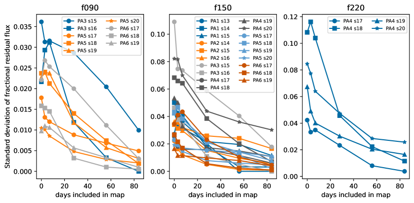
Figure 3: Standard deviation of the fractional residual flux of Uranus for every frequency and array. We bin the Uranus light curve (which has individual observation) into 3-, 7-, 28-, 56-, or 84-day bins and calculate the standard deviation. The standard deviation at zero days included in the map corresponds to the individual observations light curve, before binning.

We construct light curves of Uranus for every season, frequency channel and detector array, obtaining fluxes using the matched filter described in Section 2.2 and normalising them by the distance between Uranus and Earth. For each of these light curves we subtract its mean flux, and then divide by this mean to obtain a light curve in units of fractional residual flux. Finally, we bin it in in time intervals corresponding to the different maps we use for our sources; as detailed in Section 3: 3, 7, 28, 56, and 84 days. We create 4,000 random intervals along the length of a season, and therefore a given observation will fall inside many of these intervals. We calculate the standard deviation of the fractional residual flux over these 4,000 intervals at every frequency channel, detector array, and season. These are shown in Figure 3. As the light curve is binned into longer time intervals, the standard deviation decreases. The f090 channel has the most stable calibration, with standard deviations around a couple of percent for the three-day maps, while the f220 channel is the noisiest, reaching more than 10 per cent for the three-day maps. We also include the standard deviation of the non-binned, full light curves: this is shown at zero days included in map.

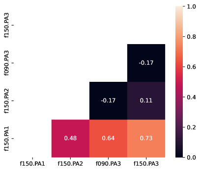
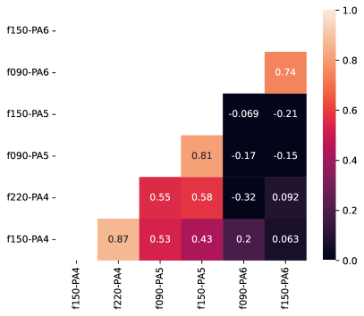
Figure 4: Pearson correlation coefficient matrix for the Uranus fractional residual light curves. The light curve from a frequency and array is correlated in time (observations taking place simultaneously) with another. On the left, the correlation for ACTPol (PA1, 2, 3), on the right the correlation for AdvACT (PA4, 5, 6).

The nature and cause of the gain fluctuations measured above can be probed by measuring the correlation between fractional residual light curves from different arrays and/or frequencies. Since the telescope scans in azimuth at a constant elevation, the two bottom arrays in the focal plane (PA1 and PA2 for ACTPol, and PA4 and PA5 for AdvACT) observe the same sky position almost simultaneously (within a few seconds of each other), whereas the top (PA3 in ACTPol and PA6 in AdvACT) will observe the same sky position at a minimum of 4 minutes earlier (later), after the sky has rotated into (out of) its field of view. Gain variations due to drifts in the detector temperatures or changes in loading from the atmosphere might therefore be manifested in differences in the correlation between the pair of arrays in the bottom row and pairs of arrays split between the top and bottom row. To test this, we bin the Uranus light curves for each array/frequency channel into one day intervals and calculate the Pearson correlation coefficient for every possible pair of light curves, only retaining bins in which both light curves in the pair had measurements.

Figure 4 shows the Pearson correlation coefficient for all combinations of frequencies and arrays, grouped into the ACTPol arrays (PA1, 2, 3; left panel) and the AdvACT arrays (PA4, 5, 6; right panel). For AdvACT, we observe a relatively high correlation between the two frequency channels in the same array. Correlations between PA4 and PA5 are also relatively high, reflecting the fact that these two arrays observe the same coordinates nearly simultaneously. However, the correlations between either PA4 or PA5 and PA6 are typically much lower. This is evidence that significant gain variations can occur on sub-day time scales, and that some of the gain variance shown in Figure 3 is from short term fluctuations rather than longer term drifts. For ACTPol (left panel of Figure 4), this pattern is less obvious (e.g., both frequencies of PA3 exhibit substantial correlation with PA1, but not with PA2). However, there are many fewer data available for ACTPol and we might not have sufficient statistics to draw conclusions. We have found evidence consistent with these results using AGN light curves rather than Uranus; this work (in preparation) will have more robust statistics since it uses scores of sources.

The above correlation test suggests that flux variations can be attributed to systematics, but we should also consider the possibility that there is intrinsic flux variation in Uranus itself. Hasselfield et al. (2013) analysed ACT observations of Uranus and compared them with the model of Griffin & Orton (1993), finding general agreement. The brightness of Uranus is probably latitude dependent, but since its sub-Earth latitude changes slowly, the mean brightness across the observed disk will vary on time scales of decades (e.g., Kramer et al., 2008) and we expect that it will remain approximately constant for the duration of an ACT season. Any flux variation is therefore expected to be dominated by the changing Earth-Uranus distance, which we know precisely and account for.

Effectively, we now have a new source of systematic error, a fractional gain error $g$ estimated as described above and shown in Figure 3. The combined new uncertainty in the flux measured for a transient map is the sum in quadrature $\Delta f^{\prime 2}=\Delta f^{2}+(sg)^{2}$, where $\Delta f$ is the uncertainty measured directly in the map and $s$ is the expected signal. By the nature of the sources we are trying to measure, we might expect for the signal to be very small and therefore $\Delta f^{\prime}\sim\Delta f$. However, we decide to use the more conservative approach where the expected signal is of the order of the $\Delta f$ uncertainty, leading to $\Delta f^{\prime}=\Delta f\sqrt{1+g^{2}}$. Based on this analysis, we multiply each error bar calculated from our matched filter maps by the factor $\sqrt{1+g^{2}}$ for all the results reported in this work.

Affiliations

¹Department of Physics, Florida State University, Tallahassee, Florida 32306, USA
²Instituto de Astrofísica and Centro de Astro-Ingeniería, Facultad de Física, Pontificia Universidad Católica de Chile, Av. Vicuña Mackenna 4860, 7820436 Macul, Santiago, Chile
³Institute of Theoretical Astrophysics, University of Oslo, Norway
⁴David A. Dunlap Department of Astronomy & Astrophysics, University of Toronto, 50 St. George St., Toronto ON M5S 3H4, Canada
⁵Specola Vaticana (Vatican Observatory), V-00120 Vatican City State
⁶School of Physics and Astronomy, Cardiff University, The Parade, Cardiff, Wales CF24 3AA, UK
⁷Department of Physics and Astronomy, University of Pennsylvania, 209 South 33rd Street, Philadelphia, Pennsylvania 19104, USA
⁸Joseph Henry Laboratories of Physics, Jadwin Hall, Princeton University, Princeton, NJ 08544
⁹Department of Astrophysical Sciences, Princeton University, Princeton, New Jersey 08544, USA
¹⁰Kavli Institute for Cosmological Physics, University of Chicago, 5640 S. Ellis Ave., Chicago, IL 60637, USA
¹¹Wits Centre for Astrophysics, School of Physics, University of the Witwatersrand, Private Bag 3, 2050, Johannesburg, South Africa
¹²School of Mathematics, Statistics & Computer Science, University of KwaZulu-Natal, Westville Campus, Durban 4041, South Africa
¹³Department of Physics, Cornell University, Ithaca, NY 14853, USA
¹⁴Department of Astronomy, Cornell University, Ithaca, NY 14853, USA
¹⁵Department of Physics and Astronomy, Haverford College, Haverford, PA, USA 19041
¹⁶Department of Physics, Stanford University, Stanford, California 94305, USA
¹⁷Kavli Institute for Particle Astrophysics and Cosmology, Stanford, CA 94305, USA
¹⁸Instituto de Física, Pontificia Universidad Católica de Valparaíso, Casilla 4059, Valparaíso, Chile
¹⁹Department of Physics, Jadwin Hall, Princeton University, Princeton, NJ 08544, USA
²⁰NASA Goddard Space Flight Center, 8800 Greenbelt Rd, Greenbelt, MD 20771, USA

References

- Abazajian et al. (2019) Abazajian K., et al., 2019, arXiv e-prints, p. arXiv:1907.04473
- Ade et al. (2019) Ade P., et al., 2019, J. Cosmology Astropart. Phys., 2019, 056
- Aiola et al. (2020) Aiola S., et al., 2020, J. Cosmology Astropart. Phys., 2020, 047
- Albareti et al. (2017) Albareti F. D., et al., 2017, ApJS, 233, 25
- Alexander et al. (2016) Alexander K. D., Berger E., Guillochon J., Zauderer B. A., Williams P. K. G., 2016, ApJ, 819, L25
- Alexander et al. (2020) Alexander K. D., van Velzen S., Horesh A., Zauderer B. A., 2020, Space Sci. Rev., 216, 81
- Berger et al. (2012) Berger E., Zauderer A., Pooley G. G., Soderberg A. M., Sari R., Brunthaler A., Bietenholz M. F., 2012, ApJ, 748, 36
- Bietenholz et al. (2021) Bietenholz M. F., Bartel N., Argo M., Dua R., Ryder S., Soderberg A., 2021, ApJ, 908, 75
- Cendes et al. (2021) Cendes Y., Alexander K. D., Berger E., Eftekhari T., Williams P. K. G., Chornock R., 2021, ApJ, 919, 127
- Choi et al. (2018) Choi S. K., et al., 2018, Journal of Low Temperature Physics, 193, 267
- Chomiuk et al. (2016) Chomiuk L., et al., 2016, ApJ, 821, 119
- D’Agostino & Pearson (1973) D’Agostino R., Pearson E. S., 1973, Biometrika, 60, 613
- D’Agostino et al. (1990) D’Agostino R. B., Belanger A., D’Agostino Jr. R. B., 1990, The American Statistician, 44, 316
- Eftekhari et al. (2022) Eftekhari T., et al., 2022, ApJ, 935, 16
- Fixsen (2009) Fixsen D. J., 2009, ApJ, 707, 916
- Gehrels et al. (2004) Gehrels N., et al., 2004, ApJ, 611, 1005
- Gezari (2021) Gezari S., 2021, ARA&A, 59
- Graham et al. (2019) Graham M. J., et al., 2019, PASP, 131, 078001
- Griffin & Orton (1993) Griffin M. J., Orton G. S., 1993, Icarus, 105, 537
- Guillochon et al. (2017) Guillochon J., Parrent J., Kelley L. Z., Margutti R., 2017, ApJ, 835, 64
- Guns et al. (2021) Guns S., et al., 2021, ApJ, 916, 98
- Harris et al. (2020) Harris C. R., et al., 2020, Nature, 585, 357
- Hasselfield et al. (2013) Hasselfield M., et al., 2013, ApJS, 209, 17
- Henderson et al. (2016) Henderson S. W., et al., 2016, Journal of Low Temperature Physics, 184, 772
- Hilton et al. (2021) Hilton M., et al., 2021, ApJS, 253, 3
- Ho et al. (2019) Ho A. Y. Q., et al., 2019, ApJ, 871, 73
- Horesh et al. (2013) Horesh A., et al., 2013, MNRAS, 436, 1258
- Huang et al. (2019) Huang K., et al., 2019, ApJ, 878, L25
- Hunter (2007) Hunter J. D., 2007, Computing in Science & Engineering, 9, 90
- Kramer et al. (2008) Kramer C., Moreno R., Greve A., 2008, A&A, 482, 359
- Krolik et al. (2016) Krolik J., Piran T., Svirski G., Cheng R. M., 2016, ApJ, 827, 127
- Laskar et al. (2013) Laskar T., et al., 2013, ApJ, 776, 119
- Laskar et al. (2018) Laskar T., et al., 2018, ApJ, 862, 94
- Laskar et al. (2019) Laskar T., et al., 2019, ApJ, 878, L26
- Levan et al. (2013) Levan A. J., Cenko S. B., Perley D. A., Tanvir N. R., 2013, GRB Coordinates Network, 14455, 1
- Lundqvist et al. (2020) Lundqvist P., et al., 2020, ApJ, 890, 159
- Lungu et al. (2022) Lungu M., et al., 2022, J. Cosmology Astropart. Phys., 2022, 044
- Naess et al. (2020) Naess S., et al., 2020, J. Cosmology Astropart. Phys., 2020, 046
- Naess et al. (2021a) Naess S., et al., 2021a, ApJ, 915, 14
- Naess et al. (2021b) Naess S., et al., 2021b, ApJ, 923, 224
- Niemack et al. (2010) Niemack M. D., et al., 2010, in Holland W. S., Zmuidzinas J., eds, Society of Photo-Optical Instrumentation Engineers (SPIE) Conference Series Vol. 7741, Millimeter, Submillimeter, and Far-Infrared Detectors and Instrumentation for Astronomy V. p. 77411S (arXiv:1006.5049), doi:10.1117/12.857464
- Nordin et al. (2019a) Nordin J., et al., 2019a, A&A, 631, A147
- Nordin et al. (2019b) Nordin J., Brinnel V., Giomi M., Santen J. V., Gal-Yam A., Yaron O., Schulze S., 2019b, Transient Name Server Discovery Report, 2019-1763, 1
- Pâris et al. (2017) Pâris I., et al., 2017, A&A, 597, A79
- Perley et al. (2014) Perley D. A., et al., 2014, ApJ, 781, 37
- Perley et al. (2019) Perley D. A., et al., 2019, MNRAS, 484, 1031
- Planck Collaboration et al. (2020) Planck Collaboration et al., 2020, A&A, 641, A6
- Predehl et al. (2021) Predehl P., et al., 2021, A&A, 647, A1
- Roth et al. (2020) Roth N., Rossi E. M., Krolik J., Piran T., Mockler B., Kasen D., 2020, Space Sci. Rev., 216, 114
- Sari (1998) Sari R., 1998, ApJ, 494, L49
- Sazonov et al. (2021) Sazonov S., et al., 2021, MNRAS, 508, 3820
- Stephens (1974) Stephens M. A., 1974, Journal of the American Statistical Association, 69, 730
- Strotjohann et al. (2015) Strotjohann N. L., et al., 2015, ApJ, 811, 117
- Sunyaev et al. (2021) Sunyaev R., et al., 2021, A&A, 656, A132
- Thornton et al. (2016) Thornton R. J., et al., 2016, ApJS, 227, 21
- Virtanen et al. (2020) Virtanen P., et al., 2020, Nature Methods, 17, 261
- Whitehorn et al. (2016) Whitehorn N., et al., 2016, ApJ, 830, 143
- Yadlapalli et al. (2022) Yadlapalli N., Ravi V., Ho A. Y. Q., 2022, ApJ, 934, 5
- Yuan et al. (2016) Yuan Q., Wang Q. D., Lei W.-H., Gao H., Zhang B., 2016, MNRAS, 461, 3375
- Zhu et al. (2021) Zhu N., et al., 2021, ApJS, 256, 23
- de Ugarte Postigo et al. (2012) de Ugarte Postigo A., et al., 2012, A&A, 538, A44
- van der Horst et al. (2014) van der Horst A. J., et al., 2014, MNRAS, 444, 3151