Generalisation Through Negation and Predicate Invention

Abstract

The ability to generalise from a small number of examples is a fundamental challenge in machine learning. To tackle this challenge, we introduce an inductive logic programming (ILP) approach that combines negation and predicate invention. Combining these two features allows an ILP system to generalise better by learning rules with universally quantified body-only variables. We implement our idea in Nopi, which can learn normal logic programs with predicate invention, including Datalog programs with stratified negation. Our experimental results on multiple domains show that our approach can improve predictive accuracies and learning times.

1 Introduction

Zendo is a game where one player, the teacher, creates a hidden rule for structures. The other players, the students, aim to discover the rule by building structures. The teacher provides feedback by marking which structures follow or break the rule without further explanation. The students continue to guess the rule. The first student to correctly guess the rule wins. For instance, consider the examples shown in Figure 1. A possible rule for these examples is “there are two red cones”.

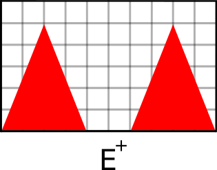
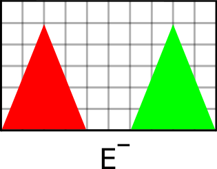
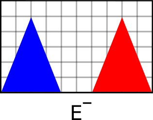
Figure 1: Positive (E⁺ ) and negative (E^-) Zendo examples.

Suppose we want to use machine learning to play Zendo, i.e. to learn rules from examples. Then we need an approach that can (i) learn explainable rules, and (ii) generalise from a small number of examples. Although crucial for many problems, these requirements are difficult for standard machine learning techniques (Cropper et al. 2022).

Inductive logic programming (ILP) (Muggleton 1991) is a form of machine learning that can learn explainable rules from a small number of examples. For instance, an ILP system could learn the following hypothesis (a set of logical rules) from the examples in Figure 1:

$$\begin{array}[]{l}\left\{\begin{array}[]{l}\emph{f(S) $\leftarrow$ cone(S,A),red(A),cone(S,B),red(B),all\_diff(A,B)}\\ \end{array}\right\}\end{array}$$

This hypothesis says that the relation f holds for the state $S$ when there are two distinct red cones $A$ and $B$, i.e. this hypothesis says there are two red cones.

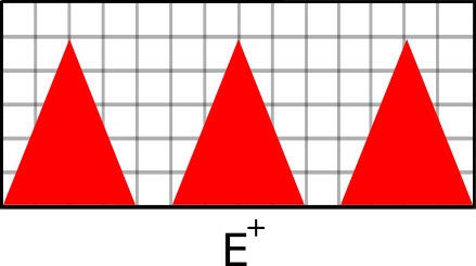
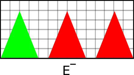
Figure 2: Additional Zendo examples.

Suppose we are given the two new examples shown in Figure 2. Our previous hypothesis does not correctly explain the new examples as it entails the new negative example. To correctly explain all the examples, we need a disjunctive hypothesis that says “[there are exactly two red cones] or [there are exactly three red cones]”. Given a new positive example with four red cones and a negative example with three red and one green cone, we would need to learn yet another rule that says “there are exactly four red cones”.

As is hopefully clear, we would struggle to generalise beyond the training examples using this approach because we need to learn a rule for each number of cones. Rather than learn a rule for each number of cones, we would ideally learn a single rule that says “all the cones are red”. However, most ILP approaches struggle to learn rules of this form because they only learn Datalog or definite programs and thus only learn rules with existentially quantified body-only variables  (Apt and Blair 1991; Dantsin et al. 2001).

To overcome this limitation, we combine negation as failure (NAF) (Clark 1977) and predicate invention (PI) (Stahl 1995) to learn rules with universally quantified body-only variables. The main reason to combine NAF and PI is that many concepts can only be expressed in this more expressive language  (Stahl 1995; Dantsin et al. 2001). For instance, for the Zendo scenario, our approach, which combines negation and PI, learns the hypothesis:

$$\begin{array}[]{l}\left\{\begin{array}[]{l}\emph{f(S) $\leftarrow$ scene(S), not inv${}_{1}$(S)}\\ \emph{inv${}_{1}$(S) $\leftarrow$ cone(S,P), not red(P)}\\ \end{array}\right\}\end{array}$$

This hypothesis says “all the cones are red”. The predicate symbol inv₁ is not provided as input and is invented by our approach. The rule defined by inv₁ says “there is a cone that is not red”. The rule defined by f negates this rule and says “it is not true that there is a cone that is not red”. The hypothesis, therefore, states “there does not exist a cone that is not red” which by the equivalences of first-order logic ($\forall\equiv\textbf{not}\ \exists\ \textbf{not}$) is the same as “all the cones are red”.

To combine negation and PI, we build on learning from failures (LFF) (Cropper and Morel 2021). An LFF learner continually generates and tests hypotheses, from which it infers constraints. For instance, if a hypothesis is too general, i.e. entails a negative example, an LFF learner, such as Popper, builds a generalisation constraint to prune more general hypotheses from the hypothesis space. We extend LFF from learning definite (monotonic) programs to learning polar programs, a fragment of normal (non-monotonic) programs. The key benefit of polar programs is that we can efficiently reason about the subsumption relation between them in our learning algorithm. Furthermore, we show (Theorem 2) that polar programs capture Datalog with stratified negation (Dantsin et al. 2001). We implement our idea in Nopi, which, as it builds on Popper, supports learning recursive and optimal programs.

Novelty, impact, and contributions.

The key novelty of our approach is the ability to learn normal logic programs with invented predicate symbols. We expand on this novelty in Section 2. The impact is that our approach can learn programs that existing approaches cannot. Specifically, we claim that combining negation and PI can improve learning performance by allowing us to learn rules with universally quantified body-only variables. Our experiments on multiple domains support our claim and show that our approach leads to vastly improved predictive accuracies and learning times.

Overall, we make the following contributions:

1. We introduce polar programs, a fragment of stratified logic programs. We show (Theorem 2) that this fragment of normal logic programs can capture Datalog with stratified negation (Dantsin et al. 2001).

2. We introduce LFF constraints for this non-monotonic setting and prove their soundness (Propositions 1 and 2).

3. We introduce Nopi, an ILP system that can learn normal logic programs with PI and recursion, such as Datalog programs with stratified negation.

4. We empirically show on multiple domains that (i) Nopi can outperform existing approaches and (ii) our non-monotonic constraints can reduce learning times.

2 Related Work

Program synthesis. ILP is a form of program synthesis (Shapiro 1983), which attracts a broad community of researchers (Evans and Grefenstette 2018; Ellis et al. 2018; Silver et al. 2022). Many recent approaches synthesise monotonic Datalog programs (Si et al. 2019; Raghothaman et al. 2020; Bembenek, Greenberg, and Chong 2023). We differ in many ways, including by learning non-monotonic programs.

Negation. Many ILP approaches learn non-monotonic programs (Quinlan 1990; Srinivasan, Muggleton, and Bain 1992; Dimopoulos and Kakas 1995; Sakama 2001; Sakama and Inoue 2009; Ray 2009). Most use negation to handle exceptions such as “birds fly except penguins” and thus require negative examples. For instance, Inoue and Kudoh (1997) learn normal logic programs by first learning a program that covers the positive examples and then adding exceptions (using NAF) to account for the negative examples. By contrast, we combine NAF and PI to improve generalisation and do not need negative examples – as Bekker and Davis (2020) state, it is sometimes necessary to learn from positive examples alone. Moreover, most approaches build on inverse entailment (Muggleton 1995), so they struggle to learn recursive and optimal programs. By contrast, our approach can learn recursive and optimal programs because we build on LFF. As Fogel and Zaverucha (1998) state, learning non-monotonic programs is difficult because the standard subsumption relation does not hold in general for normal programs. To overcome this challenge, the authors introduce a subsumption relation for normal programs based on the dependency graph of predicate symbols in a program. We differ because we introduce a general fragment of normal logic programs related to stratified logic programs. Moreover, our approach supports PI.

Predicate invention. Although crucial for many tasks, such as planning (Silver et al. 2022) and learning complex algorithms (Cropper and Muggleton 2019), most ILP systems do not support PI (Muggleton 1995; Srinivasan 2001; Blockeel and De Raedt 1998; Corapi, Russo, and Lupu 2011; Zeng, Patel, and Page 2014; Inoue, Ribeiro, and Sakama 2014). Approaches that support PI usually need metarules to restrict the syntax of hypotheses (Muggleton, Lin, and Tamaddoni-Nezhad 2015; Evans and Grefenstette 2018; Kaminski, Eiter, and Inoue 2019; Hocquette and Muggleton 2020; Dai and Muggleton 2021; Glanois et al. 2022), which, in some cases, are impossible to provide (Cropper and Tourret 2020). By contrast, we do not need metarules.

Negation and predicate invention. Ferilli (2016) describe an approach that specialises a theory to account for a misclassified negative example. If a negative example is misclassified, they introduce a conjunction of negated preconditions, where each precondition is an invented predicate. Their approach only works in a Datalog setting, cannot learn recursive programs, and only works when a negative example is misclassified. We differ because we (i) do not need negative examples, (ii) learn recursive programs, (iii) learn normal logic programs, and (iv) learn optimal programs. Siebers and Schmid (2018) learn recursive programs with negation and PI. Their approach first learns a program for the positive examples and allows some negative examples to be covered. It then flips the examples (false positives from the previous iteration are positive examples, and the previous true positives are now negative examples) and tries to learn again. We differ because we do not need negative examples or metarules. ILASP (Law, Russo, and Broda 2014) can learn non-monotonic programs with invented predicate symbols if a user tells it which symbols to invent. By contrast, Nopi does not need this information. Moreover, ILASP precomputes every possible rule in the hypothesis space, which is often infeasible. For instance, our Zendo4 experiment has approximately $10^{10}$ rules in the hypothesis space.

3 Problem Setting

We assume familiarity with logic programming (Lloyd 2012) and ASP (Gebser et al. 2012) but have included summaries in Appendix A. For clarity, we define some key terms. A normal rule is of the form $h\leftarrow b_{1},\cdots,b_{n},\mathbf{not}\ b_{n+1},\cdots,\mathbf{not}\ b_{n+m}$ where $h$ is the head atom, each $b_{i}$ is a literal, and $b_{1},\cdots,b_{n},\mathbf{not}\ b_{n+1},\cdots,\mathbf{not}\ b_{n+m}$ is the body. The symbol $\mathbf{not}$ denotes negation as failure (Clark 1977). A literal is an atom (a non-negated literal) or the negation of an atom (a negated literal). A normal logic program is a set of normal rules. A clause is a set of literals. A definite clause is a clause with exactly one non-negated literal. A substitution $\theta=\{v_{1}/t_{1},...,v_{n}/t_{n}\}$ is the simultaneous replacement of each variable $v_{i}$ by its corresponding term $t_{i}$. A clause $C_{1}$ subsumes a clause $C_{2}$ if and only if there exists a substitution $\theta$ such that $C_{1}\theta\subseteq C_{2}$ (Plotkin 1971). A definite theory $P$ subsumes a definite theory $Q$ ($P\preceq_{\theta}Q$) if and only if $\forall r_{2}\in Q,\exists r_{1}\in P$ such that $r_{1}$ subsumes $r_{2}$. A definite theory $P$ is a specialisation of a definite theory $Q$ if and only if $Q\preceq_{\theta}P$. A definite theory $P$ is a generalisation of a definite theory $Q$ if and only if $P\preceq_{\theta}Q$.

3.1 Polar Programs

To learn normal programs, we need to go beyond definite programs and standard subsumption. To do so, we introduce polar programs, which are normal programs where predicate symbols have polarities. We first define top symbols, which are head predicate symbols that are only used positively in a program:

Definition 1 (Top symbols).

Let $P$ be a normal program. Then $top(P)$ is the inclusion-maximal subset of the head predicate symbols occurring in $P$ satisfying the follow two conditions both hold:

• if $p\in top(P)$, then $p$ does not occur in a negated literal in $P$

• if $p\in top(P)$ and $p$ is in the body of a rule $r$ then the head predicate symbol of $r$ is in $top(P)$

We define defs(P) as the set of all head predicate symbols in $P$ that are not in top(P).

Example 1.

To illustrate top symbols, consider the program:

$$\begin{array}[]{l}P=\left\{\begin{array}[]{l}p\leftarrow g,q\\ p\leftarrow w,\mathbf{not}~{}s\\ g\leftarrow q,p\\ s\leftarrow l\end{array}\right\}\end{array}$$

In this program, $top(P)=\{p,g\}$ and $defs(P)=\{s\}$.

In a normal program $P$, the polarity of every head predicate symbol $p$ is positive $(pos(p))$ or negative $(neg(p))$. The polarity of a symbol in top(P) is positive. By contrast, the polarity of a symbol in defs(P) depends on whether the symbol is used positively or negatively:

Definition 2 (Polarity).

Let $P$ be a normal program, $r$ be a rule in $P$, $p$ be the head predicate symbol of $r$, $\mathit{body}^{\bm{+}}(r)$ and $\mathit{body}^{\bm{-}}(r)$ be the predicate symbols that appear in non-negated and negated body literals in $r$ respectively, and $q$ in $defs(P)$ be a predicate symbol in the body of $r$. Then the polarity of $q$ is as follows:

• if $q\in\mathit{body}^{\bm{+}}(r)$ and $pos(p)$ then $pos(q)$

• if $q\in\mathit{body}^{\bm{-}}(r)$ and $pos(p)$ then $neg(q)$

• if $q\in\mathit{body}^{\bm{+}}(r)$ and $neg(p)$ then $neg(q)$

• if $q\in\mathit{body}^{\bm{-}}(r)$ and $neg(p)$ then $pos(q)$

Example 2.

Consider the program $P$ from Example 1. The polarities of the head predicate symbols are $pos(p)$, $pos(g)$, and $neg(s)$.

We define a polar program:

Definition 3 (Polar program).

A normal program $P$ is polar if and only if the polarity of every head predicate symbol in $P$ is exclusively positive or negative.

Example 3.

The following program is not polar because the polarity of odd is neither positive nor negative:

$$\begin{array}[]{l}\left\{\emph{ ${odd}$(X) $\leftarrow$ succ(Y,X), {not}\ ${odd}$(Y)}\right\}\end{array}$$

Example 4.

The following stratified program is not polar because the polarity of $inv_{1}$ is positive and negative:

$$\begin{array}[]{l}\left\{\begin{array}[]{lll}\emph{f $\leftarrow$ inv${}_{1}$, {not}\ inv${}_{1}$}\\ \emph{inv${}_{1}$ $\leftarrow$ inv${}_{2}$}\\ \emph{inv${}_{2}$ $\leftarrow$ w}\end{array}\right\}\end{array}$$

Example 5.

The following program is polar because only $pos(unconnected)$ and $neg(inv_{1})$ hold:

$$\begin{array}[]{l}\left\{\begin{array}[]{l}\emph{$r_{1}:$ ${unconnected}(A,B)$ $\leftarrow$ {not}\ $inv_{1}$(A,B)}\\ \emph{$r_{2}:$ ${inv}_{1}$(A,B) $\leftarrow$ ${edge}$(A,B)}\\ \emph{$r_{3}:$ ${inv}_{1}$(A,B) $\leftarrow$ ${edge}$(A,C), ${inv}_{1}$(C,B)}\end{array}\right\}\end{array}$$

The rules of a polar program $P$ are positive ($P^{\bm{+}}$) or negative ($P^{\bm{-}}$) depending on the polarity of their head symbols.

Example 6.

Consider the program P from Example 5. Then $P^{\bm{+}}=\{r_{1}\}$ and $P^{\bm{-}}=\{r_{2},r_{3}\}$.

We can compare positive rules using standard subsumption. For negative rules, we need to flip the order of comparison. To do so, we introduce polar subsumption:

Definition 4 (Polar subsumption).

Let $P$ and $Q$ be polar programs. Then $P$ polar subsumes $Q$ ($P\preccurlyeq_{\diamond}Q$) iff $P^{\bm{+}}\preceq_{\theta}Q^{\bm{+}}$ and $Q^{\bm{-}}\preceq_{\theta}P^{\bm{-}}$.

Example 7.

To understand the intuition behind Definition 4, consider the following polar programs: $$P=\begin{array}[]{l}\left\{\begin{array}[]{l}\emph{$r_{1}$:\ f $\leftarrow$ {not} $inv_{1}$ }\\ \emph{$r_{2}$:\ $inv_{1}$ $\leftarrow$ a, b}\end{array}\right\}\end{array}$$ $$Q=\begin{array}[]{l}\left\{\begin{array}[]{l}\emph{$r_{3}$:\ f $\leftarrow$ {not} $inv_{1}$ }\\ \emph{$r_{4}$:\ $inv_{1}$ $\leftarrow$ a}\end{array}\right\}\end{array}$$

Note that $P\preccurlyeq_{\diamond}Q$ because $r_{1}\preceq_{\theta}r_{3}$ where $r_{1}\in P^{\bm{+}}$ and $r_{3}\in Q^{\bm{+}}$, and $r_{4}\preceq_{\theta}r_{2}$ where $r_{2}\in P^{\bm{-}}$ and $r_{4}\in Q^{\bm{-}}$ .

$$P=\begin{array}[]{l}\left\{\begin{array}[]{l}\emph{$r_{1}$:\ f $\leftarrow$ {not} $inv_{1}$ }\\ \emph{$r_{2}$:\ $inv_{1}$ $\leftarrow$ b}\\ \emph{$r_{3}$:\ $inv_{1}$ $\leftarrow$ a}\end{array}\right\}\end{array}$$

$$Q=\begin{array}[]{l}\left\{\begin{array}[]{l}\emph{$r_{4}$:\ f $\leftarrow$ {not} $inv_{1}$ }\\ \emph{$r_{5}$:\ $inv_{1}$ $\leftarrow$ b}\\ \end{array}\right\}\end{array}$$

Note that $Q\preccurlyeq_{\diamond}P$ because $r_{4}\preceq_{\theta}r_{1}$ where $r_{1}\in P^{\bm{+}}$ and $r_{4}\in Q^{\bm{+}}$, and $r_{2}\preceq_{\theta}r_{5}$ where $r_{2}\in P^{\bm{-}}$ and $r_{5}\in Q^{\bm{-}}$.

We show that polar subsumption implies entailment. Note, the properties of negation we require to prove the following two theorems hold in the commonly used semantics for NAF (such as stable and well-founded) when unstratified usage of negation does not occur. Both stratified and polar logic programs do not allow for unstratified usage of negation.

Theorem 1 (Entailment property).

Let $P$ and $Q$ be polar programs such that $P\preccurlyeq_{\diamond}Q$. Then $P\models Q$.

Proof.

For any $r_{2}$ in $Q^{\bm{+}}$ the implication trivially follows from properties of $\leq_{\theta}$. Now let $r_{1}$ in $P^{\bm{-}}$ and $r_{2}$ in $Q^{\bm{-}}$ such that $r_{2}\leq_{\theta}r_{1}$; this implies $r_{2}\models r_{1}$. By contraposition, we derive $\mathbf{not}\ r_{1}\models\mathbf{not}\ r_{2}$.

∎

We also show that polar programs can express all concepts expressible as stratified programs:

Theorem 2.

Let $S$ be a stratified logic program. Then there exists a polar program $P$ such that for all $p\in top(S)$, $S\models\forall\vec{x}.p(\vec{x})$ iff $P\models\forall\vec{x}.p(\vec{x})$ (See Appendix C).

Thus, we do not lose expressivity by learning polar programs rather than stratified programs.

3.2 Learning From Failures (LFF)

LFF searches a hypothesis space (a set of hypotheses) for a hypothesis that generalises examples and background knowledge. In the existing literature, an LFF hypothesis is a definite (monotonic) program. LFF uses hypothesis constraints to restrict the hypothesis space. Let $\mathcal{L}$ be a language that defines hypotheses. A hypothesis constraint is a constraint expressed in $\mathcal{L}$. Let $C$ be a set of hypothesis constraints written in a language $\mathcal{L}$. A hypothesis $H$ is consistent with $C$ if, when written in $\mathcal{L}$, $H$ does not violate any constraint in $C$. We denote as $\mathcal{H}_{C}$ the subset of the hypothesis space $\mathcal{H}$ which does not violate any constraint in $C$.

3.3 LFFN

We extend LFF to learn polar programs, which we call the learning from failures with negation (LFFN) setting. We define the LFFN input:

Definition 5 (LFFN input).

A LFFN input is a tuple $(E^{+},E^{-},B,\mathcal{H},C)$ where $E^{+}$ and $E^{-}$ are sets of ground atoms denoting positive and negative examples respectively; $B$ is a normal logic program denoting background knowledge; $\mathcal{H}$ is a hypothesis space of polar programs, and $C$ is a set of hypothesis constraints.

To be clear, an LFFN hypothesis is a polar (non-monotonic) program and the hypothesis space is a set of polar programs. We define an LFFN solution:

Definition 6 (LFFN solution).

Given an input tuple $(E^{+},E^{-},B,\mathcal{H},C)$, a hypothesis $H\in\mathcal{H}_{C}$ is a solution when $H$ is complete ($\forall e\in E^{+},\;B\cup H\models e$) and consistent ($\forall e\in E^{-},\;B\cup H\not\models e$).

If a hypothesis is not a solution then it is a failure. A hypothesis is incomplete when $\exists e\in E^{+},\;H\cup B\not\models e$; inconsistent when $\exists e\in E^{-},\;H\cup B\models e$; partially complete when $\exists e\in E^{+},\;H\cup B\models e$; and totally incomplete when $\forall e\in E^{+},\;H\cup B\not\models e$.

Let $cost:\mathcal{H}\mapsto\mathbb{N}$ be a function that measures the cost of a hypothesis. We define an optimal solution:

Definition 7 (Optimal solution).

Given an input tuple $(E^{+},E^{-},B,\mathcal{H},C)$, a hypothesis $H\in\mathcal{H}_{C}$ is optimal when (i) $H$ is a solution and (ii) $\forall H^{\prime}\in\mathcal{H}_{C}$, where $H^{\prime}$ is a solution, $cost(H)\leq cost(H^{\prime})$.

Our cost function is the number of literals in the hypothesis.

3.4 LFFN Constraints

An LFF learner learns hypothesis constraints from failed hypotheses. Cropper and Morel (2021) introduce hypothesis constraints based on subsumption. A specialisation constraint prunes specialisations of a hypothesis. A generalisation constraint prunes generalisations. The existing LFF constraints are only sound for monotonic programs, i.e. they can incorrectly prune optimal solutions when learning non-monotonic programs, and are thus unsound for the LFFN setting. The reason for unsoundness is that entailment is not a consequence of subsumption in a non-monotonic setting, even in the propositional case, as the following examples illustrate.

Example 8.

Consider the programs:

$$P=\begin{array}[]{l}\left\{\begin{array}[]{l}\emph{a.}\\ \emph{f $\leftarrow$ {not} $inv_{1}$ }\\ \emph{ $inv_{1}$ $\leftarrow$ b}\\ \emph{ $inv_{1}$ $\leftarrow$ a}\end{array}\right\}\end{array}$$

$$Q=\begin{array}[]{l}\left\{\begin{array}[]{l}\emph{a.}\\ \emph{f $\leftarrow$ {not} $inv_{1}$ }\\ \emph{ $inv_{1}$ $\leftarrow$ b}\\ \end{array}\right\}\end{array}$$

Note that $P\preceq_{\theta}Q$ and $Q\models f$ but $P\not\models f$. Similarly, we have the following:

$$P^{\prime}=\begin{array}[]{l}\left\{\begin{array}[]{l}\emph{a.}\\ \emph{f $\leftarrow$ {not} $inv_{1}$ }\\ \emph{ $inv_{1}$ $\leftarrow$ a, b}\end{array}\right\}\end{array}$$

$$Q^{\prime}=\begin{array}[]{l}\left\{\begin{array}[]{l}\emph{a.}\\ \emph{f $\leftarrow$ {not} $inv_{1}$ }\\ \emph{ $inv_{1}$ $\leftarrow$ a}\end{array}\right\}\end{array}$$

Note that $Q^{\prime}\preceq_{\theta}P^{\prime}$ and $P^{\prime}\models f$ but $Q^{\prime}\not\models f$.

To overcome this limitation, we introduce constraints that are optimally sound for polar programs (Definition 2) based on polar subsumption (Definition 4). In the LFFN setting, Theorem 1 implies the following propositions:

Proposition 1 (Generalisation soundness).

Let $(E^{+},E^{-},$ $B,\mathcal{H},C)$ be a LFFN input, $H_{1},H_{2}\in\mathcal{H}_{C}$, $H_{1}$ be inconsistent, and $H_{2}\preccurlyeq_{\diamond}H_{1}$. Then $H_{2}$ is not a solution.

Proposition 2 (Specialisation soundness).

Let $(E^{+},E^{-},$ $B,\mathcal{H},C)$ be a LFFN input, $H_{1},H_{2}\in\mathcal{H}_{C}$, $H_{1}$ be incomplete, and $H_{1}\preccurlyeq_{\diamond}H_{2}$. Then $H_{2}$ is not a solution.

To summarise, polar subsumption allows us to soundly prune the hypothesis space when learning non-monotonic programs. In this next section, we introduce an algorithm that uses polar subsumption to efficiently learn polar programs.

4 Algorithm

We now describe our Nopi algorithm. To aid our explanation, we first describe Popper (Cropper and Morel 2021).

Popper.

Popper takes as input an LFF input and learns hypotheses as definite programs without NAF. To generate hypotheses, Popper uses an ASP program $P$ where each model (answer set) of $P$ represents a hypothesis. Popper follows a generate, test, and constrain loop to find a solution. First, it generates a hypothesis as a solution to $P$ with the ASP system Clingo (Gebser et al. 2019). Then, Popper tests this hypothesis given the background knowledge against the training examples, typically using Prolog. If the hypothesis is a solution, Popper returns it. Otherwise, the hypothesis is a failure: Popper identifies the kind of failure and builds constraints accordingly. For instance, if the hypothesis is inconsistent, Popper builds a generalisation constraint. Popper adds these constraints to $P$ to constrain subsequent generate steps. This loop repeats until the solver finds a solution or there are no more models of $P$.

4.1 Nopi

Nopi builds on Popper and follows a generate, test, and constrain loop. The two key novelties of Nopi are its ability to (i) learn polar programs and (ii) use non-monotonic generalisation and specialisation constraints to efficiently prune the hypothesis space. We describe these advances in turn.

Polar Programs

To learn polar programs, we extend the generate ASP program to generate normal logic programs, i.e. programs with negative literals. To only generate polar programs, we add the rules and constraints of Definitions 1 and 2 to the ASP program to eliminate models where a predicate symbol has multiple polarities. The complete ASP encoding is in Appendix F, but we briefly explain it at a high-level. If a predicate symbol $p$ occurs in the body of a rule with head symbol $q$ we say $q$ calls $p$, which we name the call relation. A predicate can be called positively or negatively. We compute the transitive closure of the call relation tracking the number of negative calls on each path. If a symbol has an even number of negative calls on a path to a top symbol we say its associated rules are positive, otherwise they are negative. If any rule is labeled both positive and negative then the program is non-polar. We ignore background knowledge predicates when computing the call relation.

Polar Constraints

Nopi uses two types of constraints to prune models and thus prune hypotheses. We refer to these constraints as polar specialisation and polar generalisation constraints. These constraints differ from those used by Popper because (i) they use additional literals to assign polarity to rules, and (ii) they use polar subsumption (Definition 4) rather than standard subsumption. Polarity is important when learning polar programs because a polar generalisation constraint prunes generalisations of positive polarity rules and specialisations of negative polarity rules. A polar specialisation constraint prunes the specialisations of positive polarity rules and generalisations of negative polarity rules.

Example 9.

Reconsider the Zendo scenario from the introduction (Figures 1 and 2). The following hypothesis is incomplete as every positive example contains at least one cone:

$$h_{1}=\begin{array}[]{l}\left\{\begin{array}[]{l}\emph{$r_{1}$ : f(S) $\leftarrow$ ${scene}(S)$, {not}\ ${inv_{1}}(S)$}\\ \emph{$r_{2}$ : \ $inv_{1}(S)$ $\leftarrow$ ${cone}(S,A)$}\end{array}\right\}\end{array}$$

Since $h_{1}$ is incomplete, we can use a polar specialisation constraint to prune the hypothesis:

$$h_{2}=\begin{array}[]{l}\left\{\begin{array}[]{l}\emph{$r_{1}$ : f(S) $\leftarrow$ ${scene}(S)$, {not}\ ${inv_{1}}(S)$}\\ \emph{$r_{2}$ : \ $inv_{1}$(S) $\leftarrow$ ${cone}(S,A)$}\\ \emph{$r_{3}$ : \ $inv_{1}$(S) $\leftarrow$ ${contact}(S,A,\_)$, ${red}(A)$,}\\ \hskip 20.00003pt\emph{{not}\ ${blue}(A)$}\end{array}\right\}\end{array}$$

The hypothesis $h_{2}$ is a superset of $h_{1}$ as it includes the additional rule $r_{3}$. In $h_{2}$, the symbol $inv_{1}$ is negative because it is used negatively in $r_{1}$. Therefore, the rule $r_{3}$ implies that $h_{2}$ is a specialisation of $h_{1}$.

The polar specialisation constraint also prunes $h_{3}$:

$$h_{3}=\begin{array}[]{l}\left\{\begin{array}[]{l}\emph{$r_{4}$ : f(S) $\leftarrow$ ${scene}(S)$, {not}\ ${inv_{1}}(S)$,}\\ \hskip 48.36958pt\emph{${contact}(S,A,\_)$,${red}(A)$, ${blue}(A)$}\\ \emph{$r_{2}$ : \ $inv_{1}$(S) $\leftarrow$ ${cone}(S,A)$}\\ \end{array}\right\}\end{array}$$

The rule $r_{4}$ in $h_{3}$ adds literals to $r_{1}$ in $h_{1}$, so $h_{3}$ is a specialisation of $h_{1}$. By contrast, a polar specialisation constraint does not prune the following hypothesis:

$$h_{4}=\begin{array}[]{l}\left\{\begin{array}[]{l}\emph{$r_{1}$ : f(S) $\leftarrow$ ${scene}(S)$, {not}\ ${inv_{1}}(S)$}\\ \emph{$r_{5}$ : \ $inv_{1}$(S) $\leftarrow$ ${cone}(S,A)$, {not}\ ${red}(A)$}\end{array}\right\}\end{array}$$

Notice that the rule $r_{5}$ has an additional negated body literal compared to $r_{2}$. The symbol of this literal is neither positive nor negative, so we can ignore the occurrence of $\mathbf{not}$. Thus, $h_{4}$ is a generalisation of $h_{1}$ as the new literal occurs in the body of $r_{2}$ whose head symbol has negative polarity.

5 Experiments

To evaluate the impact of combining negation and PI, our experiments aim to answer the question:

Q1

Can negation and PI improve learning performance?

To answer Q1, we compare the performance of Nopi against Popper, which cannot negate invented predicate symbols. Comparing Nopi against different systems with different biases will not allow us to answer the question, as we would be unable to identify the reason for any performance difference. To answer Q1, we use tasks where negation and PI should be helpful, such as learning the rules of Zendo (Bramley et al. 2018). We describe the tasks in the next section.

We introduced sound constraints for polar programs to prune non-optimal solutions from the hypothesis space. To evaluate whether these constraints improve performance, our experiments aim to answer the question:

Q2

Can polar constraints improve learning performance?

To answer Q2, we compare the performance of Nopi with and without these constraints.

We introduced Nopi to go beyond existing approaches by combining negation and PI. Our experiments, therefore, aim to answer the question:

Q3

How does Nopi compare against existing approaches?

To answer Q3, we compare Nopi against Popper, Aleph, and Metagol_SN. We describe these systems below.

Questions Q1-Q3 focus on tasks where negation and PI should help. However, negation and PI are not always necessary. In such cases, can negation and PI be harmful? Our experiments try to answer the question:

Q4

Can negation and PI degrade learning performance?

To answer Q4, we evaluate Nopi on tasks where negation and PI should be unnecessary.

Reproducibility.

Experimental code may be found in the following repository: github.com/Ermine516/NOPI

Domains

We briefly describe our domains. The precise problems are found in Appendix D.

Basic (B). Non-monotonic learning tasks introduced by Siebers and Schmid (2018) and Purgał, Cerna, and Kaliszyk (2022), such as learning the definition of a leap year.

Zendo (Z). Bramley et al. (2018) introduce Zendo tasks similar to the one in the introduction.

Graphs (G). We use commonly used graph problems (Evans and Grefenstette 2018; Glanois et al. 2022), such as dominating set, independent set, and connectedness.

Sets (S). These set-based tasks include symmetric difference, decomposition into subsets, and mutual distinctness.

Systems

We compare Nopi against Popper (Cropper and Morel 2021; Cropper and Hocquette 2023), Aleph (Srinivasan 2001), and Metagol_SN (Siebers and Schmid 2018). We give Nopi and Popper identical input. The only experimental difference is the ability of Nopi to negate invented predicate symbols. Aleph can learn normal logic programs but uses a different bias than Nopi so the comparison should be interpreted as indicative only. Also, we use the default Aleph settings, but there are likely to be better settings on these datasets (Srinivasan and Ramakrishnan 2011). Metagol_SN can learn normal logic programs but requires metarules to define the hypothesis space. We use the metarules used by Siebers and Schmid (2018) supplemented with a general set of metarules (Cropper and Tourret 2020).

Experimental Setup

We use a 300s learning timeout for each task and round accuracies and learning times to integer values. We plot 99% confidence intervals. Additional experimental details are in Appendix B.

Q1. We allow all the systems to negate the given background relations. For instance, in the Zendo tasks, each system can negate colours such red. Therefore, any improvements from Nopi are not from the use of negation but from the combination of negation and PI.

Q2. We need a baseline to evaluate our polar constraints. As discussed in Section 3, Popper uses unsound constraints when learning polar programs. If a program $h$ is not a solution and has a negated invented symbol, the only sound option for Popper is to prune $h$ from the hypothesis space, but, importantly, not its generalisations or specialisations. To evaluate our polar constraints, we compare them against this simpler (banish) approach, which we call Nopi_bn. In other words, to answer Q2, we compare Nopi against Nopi_bn.

5.1 Results

Q1. Can negation and PI improve performance?

Table 1 shows the predictive accuracies of Nopi and Popper. The results show that Nopi vastly outperforms Popper regarding predictive accuracies. For instance, for all red (Z2) Popper learns:

$$\left\{\begin{array}[]{l}\emph{z(A)$\leftarrow$piece(A,B), contact(B,C), red(C), rhs(C)}\\ \emph{z(A)$\leftarrow$piece(A,B), contact(B,C), upright(C), lhs(B)}\\ \emph{z(A)$\leftarrow$piece(A,B), contact(B,C), lhs(C), lhs(B)}\\ \emph{z(A)$\leftarrow$piece(A,B), coord1(B,C), size(B,C), upright(B)}\end{array}\right\}$$

By contrast, Nopi learns:

$$\left\{\begin{array}[]{l}\emph{z(A)$\leftarrow$ scene(A), {not} $inv_{1}(A)$}\\ \emph{$inv_{1}(A)\leftarrow$ piece(A,B), {not} red(B)}\end{array}\right\}$$

Table 2 shows the corresponding learning times. The results show that Nopi rarely needs more than 40s to learn a solution. One of the more difficult problems (30s to learn) is largest is red (Z6), which involves inventing two predicate symbols and having two layers of negation, which, as far as we are aware, goes beyond anything in the existing literature:

$$\left\{\begin{array}[]{l}\emph{zendo(A) $\leftarrow$ {scene}(A), piece(A,B), {not}\ $inv_{1}(B,A)$}\\ \emph{$inv_{1}(A,B)$ $\leftarrow$ piece(B,C), size(C,D), {not}\ $inv_{2}(D,A)$}\\ \emph{$inv_{2}(A,B)$ $\leftarrow$ size(B,C), red(B), $A\leq C$}\par\end{array}\right\}$$

Popper sometimes terminates in less than a second. The reason is that on some problems, because of its highly efficient search, Popper almost immediately proves that there is no monotonic solution.

Overall, the results from this section suggest that the answer to Q1 is that combining negation and PI can drastically improve learning performance.

Task	Nopi	Popper	Aleph	MetagolSN
B1	100 $\pm$ 0	82 $\pm$ 0	50 $\pm$ 0	0 $\pm$ 0
B2	100 $\pm$ 0	0 $\pm$ 0	50 $\pm$ 0	100 $\pm$ 0
B3	100 $\pm$ 0	82 $\pm$ 0	82 $\pm$ 0	100 $\pm$ 0
Z1	100 $\pm$ 0	0 $\pm$ 0	60 $\pm$ 0	0 $\pm$ 0
Z2	100 $\pm$ 0	55 $\pm$ 0	67 $\pm$ 0	0$\pm$ 0
Z3	100 $\pm$ 0	0 $\pm$ 0	65 $\pm$ 0	0 $\pm$ 0
Z4	100 $\pm$ 0	55 $\pm$ 0	58 $\pm$ 0	0$\pm$ 0
Z5	100 $\pm$ 0	0 $\pm$ 0	21 $\pm$ 0	0 $\pm$ 0
Z6	100 $\pm$ 0	0 $\pm$ 0	45 $\pm$ 0	0 $\pm$ 0
G1	100 $\pm$ 0	0 $\pm$ 0	50 $\pm$ 0	0 $\pm$ 0
G2	100 $\pm$ 0	24 $\pm$ 0	47 $\pm$ 0	0 $\pm$ 0
G3	100 $\pm$ 0	0 $\pm$ 0	12 $\pm$ 0	0 $\pm$ 0
G4	100 $\pm$ 0	20 $\pm$ 0	100 $\pm$ 0	0 $\pm$ 0
G5	100 $\pm$ 0	0 $\pm$ 0	50 $\pm$ 0	0 $\pm$ 0
G6	100 $\pm$ 0	0 $\pm$ 0	21 $\pm$ 0	0 $\pm$ 0
G7	100 $\pm$ 0	0 $\pm$ 0	50 $\pm$ 0	0 $\pm$ 0
G8	100 $\pm$ 0	0 $\pm$ 0	50 $\pm$ 0	0 $\pm$ 0
S1	100 $\pm$ 0	0 $\pm$ 0	50 $\pm$ 0	0 $\pm$ 0
S2	100 $\pm$ 0	0 $\pm$ 0	50 $\pm$ 0	0 $\pm$ 0
S3	92 $\pm$ 0	0 $\pm$ 0	57 $\pm$ 0	0 $\pm$ 0
S4	100 $\pm$ 0	0 $\pm$ 0	50 $\pm$ 0	0 $\pm$ 0
S5	100 $\pm$ 0	57 $\pm$ 0	23 $\pm$ 0	0 $\pm$ 0
S6	100 $\pm$ 0	0 $\pm$ 0	0 $\pm$ 0	0 $\pm$ 0

Table 1: Mean predictive accuracies (10 runs).

Task	Nopi	Popper	Aleph	MetagolSN
B1	20 $\pm$ 0	timeout	20 $\pm$ 0	timeout
B3	3 $\pm$ 0	0 $\pm$ 0	18 $\pm$ 2	1 $\pm$ 0
Z1	2 $\pm$ 0	0 $\pm$ 0	7$\pm$ 1	timeout
Z2	12 $\pm$ 0	1 $\pm$ 0	95 $\pm$ 2	timeout
Z3	2 $\pm$ 0	0 $\pm$ 0	27 $\pm$ 1	timeout
Z4	22 $\pm$ 1	0 $\pm$ 0	20 $\pm$ 1	timeout
Z5	15 $\pm$ 1	0 $\pm$ 0	24 $\pm$ 1	timeout
Z6	67 $\pm$ 4	0 $\pm$ 0	149 $\pm$ 24	timeout
G1	4 $\pm$ 0	0 $\pm$ 0	32 $\pm$ 2	timeout
G2	2 $\pm$ 0	0 $\pm$ 0	0 $\pm$ 0	timeout
G3	9 $\pm$ 0	16 $\pm$ 0	1 $\pm$ 0	timeout
G4	12 $\pm$ 0	0 $\pm$ 0	1 $\pm$ 0	timeout
G5	8 $\pm$ 0	0 $\pm$ 0	0 $\pm$ 0	timeout
G6	19 $\pm$ 3	0 $\pm$ 0	12 $\pm$ 1	timeout
G7	58 $\pm$ 8	0 $\pm$ 0	12 $\pm$ 1	timeout
G8	71 $\pm$ 9	0 $\pm$ 0	38 $\pm$ 1	timeout
S2	3 $\pm$ 0	0 $\pm$ 0	1 $\pm$ 0	timeout
S4	28 $\pm$ 2	0 $\pm$ 0	0 $\pm$ 2	0 $\pm$ 0
S5	43 $\pm$ 3	0 $\pm$ 0	23 $\pm$ 3	timeout
S6	3 $\pm$ 0	0 $\pm$ 0	1 $\pm$ 0	timeout

Table 2: Mean learning times (10 runs). We only show tasks where the times of Nopi and Popper differ by more than 1 second.

Q2. Can polar constraints improve performance?

Table 3 shows the learning times of Nopi and Nopi_bn. The results show that Nopi has lower learning times than Nopi_bn. In other words, the results show that polar constraints can drastically reduce learning times. A wilcoxon signed-rank test confirms the significance of the differences at the $p<10^{-8}$ value. For simpler tasks, there is little benefit from the polar constraints as the overhead of constructing and adding them to the solver negates the pruning benefits. For more difficult tasks, the difference is substantial. For instance, the learning times for Nopi and Nopi_bn on the sym. difference (S4) task are 31s and 72s respectively, a 57% reduction. Overall, the results suggest that the answer to Q2 is that our polar constraints can drastically reduce learning times.

Task	Nopi	Nopibn	Change
B3	2 $\pm$ 0	4 $\pm$ 0	-50%
Z4	11 $\pm$ 1	49 $\pm$ 2	-78%
Z5	13 $\pm$ 1	29 $\pm$ 1	-55%
Z6	30 $\pm$ 1	115 $\pm$ 9	-74%
G2	1 $\pm$ 0	9 $\pm$ 0	-89%
G3	18 $\pm$ 1	23 $\pm$ 1	-22%
G4	20 $\pm$ 3	68 $\pm$ 4	-71%
G5	3 $\pm$ 0	11 $\pm$ 0	-73%
G6	23 $\pm$ 1	33 $\pm$ 3	-27%
G7	56 $\pm$ 5	93 $\pm$ 9	-40%
G8	63 $\pm$ 5	103 $\pm$ 9	-39%
S3	3 $\pm$ 0	13 $\pm$ 0	-77%
S4	31 $\pm$ 2	72 $\pm$ 9	-57%
S5	35 $\pm$ 2	53 $\pm$ 5	-34%
S6	4 $\pm$ 0	8 $\pm$ 1	-50%

Table 3: Mean learning time (125 runs). We only show tasks where the times differ by more than 1 second.

Q3. How does Nopi compare against existing approaches?

Table 1 shows the predictive accuracies of the systems. As is clear, Nopi overwhelmingly outperforms the other systems. This result is expected. Besides Metagol_SN, the other systems cannot learn normal logic programs with PI. Aleph can learn programs with NAF and sometimes learns reasonable solutions. However, Aleph cannot perform PI so, due to its restricted language, it struggles to generalise. In many cases, Aleph simply memorises the training examples. Because it relies on user-supplied metarules, Metagol_SN can only learn normal logic programs of a very restricted syntactic structure and thus struggles on almost all our tasks. Overall, the results from this section suggest that the answer to Q3 is that Nopi performs well compared to other approaches on problems that need negation and PI.

Q4. Can negation and PI degrade performance?

The Appendix includes tables showing the predictive accuracies and learning times of the systems. The results show that Nopi performs worse than Popper on these tasks. The Blumer bound (Blumer et al. 1987) helps explain why. According to the bound, given two hypotheses spaces of different sizes, searching the smaller space should result in higher predictive accuracy compared to searching the larger one if the target hypothesis is in both. Nopi considers programs with negation and PI and thus searches a drastically larger hypothesis space than Popper and the other systems. The tasks in Q4 do not need negation and PI, thus explaining the difference.

6 Conclusions and Limitations

We have introduced an approach that combines negation and PI. Our approach can learn polar programs, including stratified Datalog programs (Theorem 2). We introduced generalisation and specialisation constraints for this non-monotonic fragment and showed that they are optimally sound (Theorem 1). We introduced Nopi, an ILP system that can learn normal logic programs with PI, including recursive programs. We have empirically shown on multiple domains that (i) Nopi can outperform existing approaches, and (ii) our non-monotonic constraints can reduce learning times.

Limitations and Future Work

Inefficient constraints. Nopi sometimes spends 30% of learning time building polar constraints. This inefficiency is an implementation issue rather than a theoretical one. Therefore, our empirical results likely underestimate the performance of Nopi, especially the improvements from using polar constraints.

Unnecessary negation and PI. Our results show that combining negation and PI allows Nopi to learn programs that other approaches cannot. However, the results also show that this increased expressivity can be detrimental when the combination of negation and PI is unnecessary. Thus, the main limitation of this work and direction for future work is to automatically detect when a problem needs negation and PI.

Appendix A Terminology

A.1 Logic Programming

We assume familiarity with logic programming (Lloyd 2012) but restate some key relevant notation. A variable is a string of characters starting with an uppercase letter. A predicate symbol is a string of characters starting with a lowercase letter. The arity $n$ of a function or predicate symbol is the number of arguments it takes. An atom is a tuple $p(t_{1},...,t_{n})$, where $p$ is a predicate of arity $n$ and $t_{1}$, …, $t_{n}$ are terms, either variables or constants. An atom is ground if it contains no variables. A literal is an atom or the negation of an atom. A clause is a set of literals. A clausal theory is a set of clauses. A constraint is a clause without a non-negated literal. A definite clause is a clause with exactly one non-negated literal. A program is a set of definite clauses. A substitution $\theta=\{v_{1}/t_{1},...,v_{n}/t_{n}\}$ is the simultaneous replacement of each variable $v_{i}$ by its corresponding term $t_{i}$. A clause $c_{1}$ subsumes a clause $c_{2}$ if and only if there exists a substitution $\theta$ such that $c_{1}\theta\subseteq c_{2}$. A program $h_{1}$ subsumes a program $h_{2}$, denoted $h_{1}\preceq h_{2}$, if and only if $\forall c_{2}\in h_{2},\exists c_{1}\in h_{1}$ such that $c_{1}$ subsumes $c_{2}$. A program $h_{1}$ is a specialisation of a program $h_{2}$ if and only if $h_{2}\preceq h_{1}$. A program $h_{1}$ is a generalisation of a program $h_{2}$ if and only if $h_{1}\preceq h_{2}$.

A.2 Answer Set Programming

We also assume familiarity with answer set programming (Gebser et al. 2012) but restate some key relevant notation (Law, Russo, and Broda 2014). A literal can be either an atom $p$ or its default negation $\text{not }p$ (often called negation by failure). A normal rule is of the form $h\leftarrow b_{1},...,b_{n},\text{not }c_{1},...\text{not }c_{m}$. where $h$ is the head of the rule, $b_{1},...,b_{n},\text{not }c_{1},...\text{not }c_{m}$ (collectively) is the body of the rule, and all $h$, $b_{i}$, and $c_{j}$ are atoms. A constraint is of the form $\leftarrow b_{1},...,b_{n},\text{not }c_{1},...\text{not }c_{m}.$ where the empty head means false. A choice rule is an expression of the form $l\{h_{1},...,h_{m}\}u\leftarrow b_{1},...,b_{n},\text{not }c_{1},...\text{not }c_{m}$ where the head $l\{h_{1},...,h_{m}\}u$ is called an aggregate. In an aggregate, $l$ and $u$ are integers and $h_{i}$, for $1\leq i\leq m$, are atoms. An answer set program $P$ is a finite set of normal rules, constraints, and choice rules. Given an answer set program $P$, the Herbrand base of $P$, denoted as ${HB}_{P}$, is the set of all ground (variable free) atoms that can be formed from the predicates and constants that appear in $P$. When $P$ includes only normal rules, a set $A\in{HB}_{P}$ is an answer set of $P$ iff it is the minimal model of the reduct $P^{A}$, which is the program constructed from the grounding of $P$ by first removing any rule whose body contains a literal $\text{not }c_{i}$ where $c_{i}\in A$, and then removing any defaultly negated literals in the remaining rules. An answer set $A$ satisfies a ground constraint $\leftarrow b_{1},...,b_{n},\text{not }c_{1},...\text{not }c_{m}.$ if it is not the case that $\{b_{1},...,b_{n}\}\in A$ and $A\cap\{c_{1},...,c_{m}\}=\emptyset$.

Appendix B Additional Experimental Details

We enforce a timeout of 10 minutes per task. We measure predictive accuracy and learning time. We measure the mean and standard error over 10 trials. We use an 8-Core 1.6 GHz Intel Core i5 and a single CPU.

Appendix C Theorem 2 Proof: Stratified to Polar

In this section, we show that stratified normal logic programs can be transformed into polar programs. Before defining what a stratified program is, we need a few definitions. Given a normal logic program $P$, we define $H(P)=top(P)\cup defs(P)$, and for any rule $r\in P$, the head symbol of $r$ will be denoted by $head_{s}(r)$. Stratified normal logic programs are defined as follows:

Definition 8.

A normal logic program program $S$ is stratified if there exists a total function $\mu:H(S)\rightarrow\mathbb{N}$ such that for all $p\in H(S)$ and $r\in S$:

• if $p\in\mathit{body}^{\bm{+}}(r)$, then $\mu(head_{s}(r))\geq\mu(p)$

• if $p\in\mathit{body}^{\bm{-}}(r)$, then $\mu(head_{s}(r))>\mu(p)$

This definition prunes normal logic programs with unstratified use of negation, for example, $odd(X)\leftarrow succ(Y,X),\mathbf{not}\ odd(Y)$. Notice that Definition 8 requires $\mu(odd)>\mu(odd)$, but this is impossible. To transform a stratified normal logic program $S$ into a polar program $S^{\prime}$, we enforce the following properties on $S^{\prime}$:

• For every $p\in H(S^{\prime})$, $p$ is annotated exclusively $pos(p)$ or $neg(p)$ within $S^{\prime}$

Notice that if we annotate a stratified program $S$, every symbol in $H(S)$ will be annotated. Only programs with unstratified negation contain symbols that cannot be annotated.

To simplify the arguments in the proof below, we will define $ann(p)\in\{\bm{+},\bm{-}\}$ for $p\in H(S^{\prime})$, which denotes that where $pos(p)$ holds ($\bm{+}$) and/or $neg(p)$ holds($\bm{-}$). Additionally, we define the function $\bowtie:\{\bm{+},\bm{-}\}\rightarrow\{\bm{+},\bm{-}\}$ which behaves as follows:

$$x\bowtie y=\left\{\begin{array}[]{cc}\bm{+}&x=y\\ \bm{-}&x\not=y\end{array}\right.$$

In addition, we require the following concepts:

Definition 9.

Let $S$ be a set of rules. Then

$$\mathit{sym}_{T}(S)=\{head_{s}(c)|c\in S\}.$$

Definition 10.

Let $S$ be a set of rules and $p$ and $q$ predicate symbols. Then $S[p\setminus q]$ denotes the set of rules where every occurrence of $p$ is replaced by an occurrence of $q$.

We transform stratified programs into polar programs by introducing fresh names and duplicating rules. We illustrate the process below and show that polar programs are indeed as expressive as stratified normal logic programs.

C.1 Flattening

Definition 11.

Let $S$ be a stratified program, $c_{1},c_{2}\in S$, and $p\in H(S)$ such that $p\in\mathit{body}^{\bm{+}}(c_{1})$, $p\in\mathit{body}^{\bm{-}}(c_{2})$, and $head_{s}(c_{1})\not=p$. Then the program $S^{\prime}=$

$$S\setminus\{c_{1}\}\cup\{c_{1}\}[p\setminus p^{\prime}]\cup\{c|head_{s}(c)=p\wedge c\in S\}[p\setminus p^{\prime}]$$

is a $p$-flattening of $S$ where $p^{\prime}$ is fresh in $S$. We denote the $p$-flattening of $S$ into $S^{\prime}$ by $S\rightharpoonup_{p}S^{\prime}$ and let $\mathit{flat}(S)$ denote the set of $p\in H(S)$ for which a $p$-flattening of $S$ exists.

Example 10.

Note that for the following program $S$, $\mathit{flat}(S)=\{\mathtt{inv_{1}}\}$ and

$$\mathtt{f}\leftarrow\ \mathtt{inv_{1}},\mathbf{not}\ \mathtt{inv_{1}}.$$

$$\mathtt{inv_{1}}\leftarrow\ \mathtt{inv_{3}}.$$

$$\mathtt{inv_{3}}\leftarrow\ \mathtt{p}.$$

the $\mathtt{inv_{1}}$-flattening of $S$ results in the program $S^{\prime}$ as follows

$$\mathtt{f}\leftarrow\ \mathtt{inv_{2}},\mathbf{not}\ \mathtt{inv_{1}}.$$

$$\mathtt{inv_{1}}\leftarrow\ \mathtt{inv_{3}}.$$

$$\mathtt{inv_{2}}\leftarrow\ \mathtt{inv_{3}}.$$

$$\mathtt{inv_{3}}\leftarrow\ \mathtt{p}.$$

lemma 1.

Let $S,S^{\prime}$ be stratified programs such that $S\rightharpoonup_{p}S^{\prime}$ and $p^{\prime}\in\mathit{sym}_{T}(S^{\prime})\setminus\mathit{sym}_{T}(S)$. Then $p^{\prime}\not\in\mathit{flat}(S^{\prime})$.

Proof.

The symbol $p^{\prime}$ only occurs positively in $S^{\prime}$ and thus cannot be a member of $\mathit{flat}(S^{\prime})$ by definition. ∎

lemma 2.

Let $S_{0}$ be a stratified program such that $p\in\mathit{flat}(S)$. Then there $\exists n>0$ such that $S_{0}\rightharpoonup_{p}S_{1}\rightharpoonup_{p}\cdots\rightharpoonup_{p}S_{n}$ and $p\not\in\mathit{flat}(S_{n})$.

Proof.

The process of $p$-flattening replaces one occurrence of $p\in\mathit{body}^{\bm{+}}(c)$ for $c\in S_{i}$, such that $head_{s}(c)\not=p$, by a fresh symbol thus $S_{i+1}$ has one less occurrence of $p$. After finitely many steps $n$ every occurrence of $p\in\mathit{body}(c)$ for $c\in S_{n}$ such that $head_{s}(c)\not=p$ will occur in $p\in\mathit{body}^{\bm{-}}(c)$. ∎

We say $S>_{f}S^{\prime}$ if there exists $p\in\mathit{flat}(S)$ such that $S\rightharpoonup_{p}S^{\prime}$. The transitive-reflexive closure is denoted by $\geq_{f}^{*}$.

lemma 3.

Let $S$ be a stratified program. Then there exists $S^{\prime}$ such that $S\geq_{f}^{*}S^{\prime}$ and $\mathit{flat}(S^{\prime})=\emptyset$.

Proof.

Follows from induction on the size of $\mathit{flat}(S)$. The basecase is trivial, and the stepcase follows from Lemma 2. ∎

We refer to a stratified program $S$ such that $\mathit{flat}(S)=\emptyset$ as semi-polar.

Example 11.

The program from Example 10 is semi-polar but not polar, that is

$$\mathtt{f}\leftarrow\ \mathtt{inv_{2}},\mathbf{not}\ \mathtt{inv_{1}}.$$

$$\mathtt{inv_{1}}\leftarrow\ \mathtt{inv_{3}}.$$

$$\mathtt{inv_{2}}\leftarrow\ \mathtt{inv_{3}}.$$

$$\mathtt{inv_{3}}\leftarrow\ \mathtt{p}.$$

Semi-polar programs have property (1) mentioned at the beginning of this section. In the following subsection, we show how to transform semi-polar programs into programs that also have property (2).

C.2 Stretching

In order to transform semi-polar programs into polar ones, we need to rename symbols with multiple trace values:

Definition 12.

Let $S$ be semi-polar, $x\in\{\bm{+},\bm{-}\}$ $r\in S$, $p\in H(S)$, and $l$ a literal of $r$ such that the symbol of $l$ is $p$. We define the trace of $p$ from $r$, denoted $\mathit{tr}_{S}(r,p)$, as follows:

• if $p\in\mathit{body}^{x}(r)$ and for all $r^{\prime}\in S$, $head_{s}(r)\not\in\mathit{body}(r^{\prime})$,
  then $\mathit{tr}_{S}(r,p)=x$

• if $p\in\mathit{body}^{x}(r)$, $head_{s}(r)\in\mathit{body}(r^{\prime})$ and $p\not=head_{s}(r)$,
  then $\mathit{tr}_{S}(r,p)=x\bowtie\mathit{tr}_{S}(r^{\prime},head_{s}(r))$

• if $p=head_{s}(r)$, $p\in\mathit{body}(r^{\prime})$, and $head_{s}(r^{\prime})\not=p$,
  then $\mathit{tr}_{S}(r,p)=\mathit{tr}_{S}(r^{\prime},p)$

• otherwise, $\mathit{tr}_{S}(r,p)=\bm{+}.$

Example 12.

The program from Example 11 has the following traces

$$\mathit{tr}_{S}(4,\mathtt{inv_{3}})=\mathit{tr}_{S}(3,\mathtt{inv_{3}})=\bm{+}\bowtie\mathit{tr}_{S}(1,\mathtt{inv_{2}})=\bm{+}$$

$$\mathit{tr}_{S}(4,\mathtt{inv_{3}})=\mathit{tr}_{S}(2,\mathtt{inv_{3}})=\bm{+}\bowtie\mathit{tr}_{S}(1,\mathtt{inv_{1}})=\bm{-}$$

$$\mathit{tr}_{S}(3,\mathtt{inv_{3}})=\bm{+}\bowtie\mathit{tr}_{S}(1,\mathtt{inv_{2}})=\bm{+}\bowtie\bm{+}=\bm{+}$$

$$\mathit{tr}_{S}(2,\mathtt{inv_{3}})=\bm{+}\bowtie\mathit{tr}_{S}(1,\mathtt{inv_{1}})=\bm{+}\bowtie\bm{-}=\bm{-}$$

$$\mathit{tr}_{S}(3,\mathtt{inv_{2}})=\mathit{tr}_{S}(1,\mathtt{inv_{2}})=\bm{+}$$

$$\mathit{tr}_{S}(2,\mathtt{inv_{1}})=\mathit{tr}_{S}(1,\mathtt{inv_{1}})=\bm{-}$$

where rules are numbered as below:

$$1:\mathtt{f}\leftarrow\ \mathtt{inv_{2}},\mathbf{not}\ \mathtt{inv_{1}}.$$

$$2:\mathtt{inv_{1}}\leftarrow\ \mathtt{inv_{3}}.$$

$$3:\mathtt{inv_{2}}\leftarrow\ \mathtt{inv_{3}}.$$

$$4:\mathtt{inv_{3}}\leftarrow\ \mathtt{p}.$$

Notice that $\mathtt{inv_{3}}$ has multiple trace values depending on where one starts the trace.

Note that for both stratified and semi-polar programs, $\mathit{tr}_{S}(c,p)$ may return multiple values for the same symbol $p$ as the symbol of $c$ influences the result. For semi-polar programs, $\mathit{tr}_{S}(c,p)$ where $head_{s}(c)=p$ may also be problematic as the value of $\mathit{tr}_{S}(c,p)$ is dependent on which rule $c^{\prime}$ we choose. Thus, we avoid recursive rules when defining $p$-stretching below.

Definition 13.

Let $S$ be semi-polar, $c_{1},c_{2}\in S$, and $p\in H(S)$ such that $p\in\mathit{body}(c_{1})\cap\mathit{body}(c_{2})$, $\mathit{tr}_{S}(c_{1},p)\not=\mathit{tr}_{S}(c_{2},p)$ , and $head_{s}(c_{1})\not=head_{s}(c_{2})\not=p$. Then $S^{\prime}=$

$$S\setminus\{c_{1}\}\cup\{c_{1}\}[p\setminus p^{\prime}]\cup\{c|head_{s}(c)=p\wedge c\in S\}[p\setminus p^{\prime}]$$

is a $p$-stretching of $S$ where $p^{\prime}$ is fresh in $S$. We denote the $p$-stretching of $S$ into $S^{\prime}$ by $S\rightharpoondown_{p}S^{\prime}$ and let $\mathit{stret}(S)$ denote the set of $p\in H(S)$ for which a $p$-stretching of $S$ exists.

Example 13.

The program from Example 12, denoted as $S$, has $\mathit{stret}(S)=\{\mathtt{inv_{3}}\}$. The $\mathtt{inv_{3}}$-stretching results in the following program

$$\mathtt{f}\leftarrow\ \mathtt{inv_{2}},\mathbf{not}\ \mathtt{inv_{1}}.$$

$$\mathtt{inv_{1}}\leftarrow\ \mathtt{inv_{3}}.$$

$$\mathtt{inv_{2}}\leftarrow\ \mathtt{inv_{4}}.$$

$$\mathtt{inv_{3}}\leftarrow\ \mathtt{p}.$$

$$\mathtt{inv_{4}}\leftarrow\ \mathtt{p}.$$

Notice that the resulting program has unique trace values for each symbol, and the program is polarized. For larger programs, this process requires more steps. We formalize it using the following lemmas.

lemma 4.

Let $S,S^{\prime}$ be semi-polar such that $S\rightharpoondown_{p}S^{\prime}$ and $p^{\prime}\in\mathit{sym}_{T}(S^{\prime})\setminus\mathit{sym}_{T}(S)$. Then $p^{\prime}\not\in\mathit{stret}(S^{\prime})$.

Proof.

$p^{\prime}$ only occurs once and thus has a unique trace. ∎

lemma 5.

Let $S$ be semi-polar such that $p\in\mathit{stret}(S)$. Then there $\exists n>0$ such that $S\rightharpoondown_{p}S_{1}\rightharpoondown_{p}\cdots\rightharpoondown_{p}S_{n}$ and $p\not\in\mathit{stret}(S_{n})$.

Proof.

The process of $p$-stretching replaces one occurrence of $p\in\mathit{body}^{\bm{+}}(c)$ for $c\in S_{i}$, such that $head_{s}(c)\not=p$, by a fresh symbol thus $S_{i+1}$ has one less occurrence of $p$. After finitely many steps $n$, every occurrence of $p\in\mathit{body}(c)$ for $c\in S_{n}$ will have the same trace. ∎

We say $S>_{s}S^{\prime}$ if there exists $p\in\mathit{stret}(S)$ such that $S\rightharpoondown_{p}S^{\prime}$. The transitive-reflexive closure is denoted by $\geq_{s}^{*}$.

lemma 6.

Let $S$ be semi-polar. Then there exists $S^{\prime}$ such that $S\geq_{s}^{*}S^{\prime}$ and $\mathit{stret}(S^{\prime})=\emptyset$.

Proof.

Follows from induction on the size of $\mathit{stret}(S)$. The basecase is trivial, and the stepcase follows from Lemma 5. ∎

lemma 7.

Let $S,S^{\prime}$ be semi-polar programs such that $S\geq_{s}^{*}S^{\prime}$ and $\mathit{stret}(S^{\prime})=\emptyset$. Then $S^{\prime}$ is polar.

Proof.

It is easy to verify that $ann(p)=\mathit{tr}_{S^{\prime}}(c,p)$ where $p\in\mathit{body}(c)$ and $p\in H(S^{\prime})$. ∎

Let $S$ be a stratified normal program, $S^{\prime}$ a semi-polar program such that $S\geq_{f}^{*}S^{\prime}$ and $S^{\prime\prime}$ a polar program such that $S^{\prime}\geq_{s}^{*}S^{\prime\prime}$. Then we refer to $S^{\prime\prime}$ as the polarisation of $S$, denoted $\mathit{pol}(S)$.

Theorem 3.

Let $S$ be a stratified normal program and $p\in H(S)$. Then $S\models\forall\vec{x}.p(\vec{x})$ iff $\mathit{pol}(S)\models\forall\vec{x}.p(\vec{x})$.

Proof.

This follows from the fact that flattening and stretching only introduces fresh symbols that duplicate existing predicate definitions. Thus, $\mathit{pol}(S)$ contains many repetitions, modulo renaming, of the predicate definitions contained in $S$. ∎

The formulation in the main body of the paper follows from the above theorem as $top(S)\subseteq H(S)$ and $P=\mathit{pol}(S)$.

Theorem 4.

Let $S$ be a stratified logic program. Then there exists a polar program $P$ such that for all $p\in top(S)$, $S\models\forall\vec{x}.p(\vec{x})$ iff $P\models\forall\vec{x}.p(\vec{x})$.

Appendix D Problems Table 3: Solutions

Here we provide found solutions for the problems found in Table 3. We include the solutions found by Nopi, Nopi_bn, Aleph, and Metagol_sn. Note Metagol_sn only found solutions for Stepwise-narrowing problems.

D.1 Basic

• B1:Divides Entire List is there a number in the list A which divides every number in the list

  Nopi & Nopi_bn

  divlist(A):- member(B,A), not inv1(B,A).
   inv1(A,B):- member(C,B), not my_div(A,B).
      
  

  Popper

  divlist(A):- head(A,C),tail(A,B),
  member(D,B), my_div(C,D).
      
  

  Aleph

   divlist([11,33,44,121]).
   divlist([6,9,18,3,27]).
   divlist([2,4,6,8,10,12,14]).
      
  

D.2 Step-Wise Narrowing Tasks

• B2: 1 of 2 even is one of the numbers A or B even

  Nopi & Nopi_bn

   one_even(A,B) :- even(A), not inv1(B,A).
   one_even(A,B) :- even(B), not inv1(B,A).
       inv1(A,B) :- even(B),even(A).
      
  

  Aleph

  one_even(3,18). one_even(2,5).
  one_even(3,4).  one_even(2,3).
  one_even(3,2).  one_even(1,4).
  one_even(1,2).
      
  

  Metagol_sn

    one_even(A,B) :-  even(A), not _one_even(A,B).
    one_even(A,B) :-  even(B), not __one_even(A,B).
   _one_even(A,B) :- even(B).
  __one_even(A,B) :- even(A).
  

• B3: Leapyear is A a leap year

  Nopi & Nopi_bn

  leapyear(A):- divisible4(A), not inv1(A).
  inv1(A):-  divisible100(A), not inv2(A).
  inv2(A):- divisible400(A).
      
  

  Aleph

  leapyear(996). leapyear(988).  leapyear(984).
  leapyear(980).  leapyear(972).  leapyear(968).
  leapyear(964).  leapyear(956).  leapyear(952).
  leapyear(948).  leapyear(940).  leapyear(936).
  leapyear(932).  leapyear(924).  leapyear(920).
  leapyear(916).  leapyear(908).  leapyear(904).
  ... ’341 more positive instances’
  leapyear(A):-divisible16(A).
  leapyear(1004).
  

  Metagol_sn

    leapyear(A) :- div4(A), not _leapyear(A).
   _leapyear(A) :- div100(A), not __leapyear(A)).
  __leapyear(A) :- div400(A).
  

D.3 Zendo

• Z1: Nothing is upright none of the cones in the scene A are upright.

  Nopi & Nopi_bn

   zendo(A) :- not inv1(A).
    inv1(A) :- piece(A,B),upright(B).
      
  

  Aleph

  zendo(A):-piece(A,B),size(B,C),small(C),
  blue(B),not upright(B).
  
  zendo(D):-piece(D,E),lhs(E),blue(E),
  piece(D,F),green(F).
      
  

• Z2: All red cones are all cones in the scene A red

  Nopi & Nopi_bn

  zendo(A) :- not inv1(A).
   inv1(A) :- piece(A,B), not red(B).
      
  

  Popper

  zendo(A):- piece(A,B),contact(B,C),
  red(C), rhs(C).
  
  zendo(A):- piece(A,B),contact(B,C),
  upright(C), lhs(B).
  
  zendo(A):- piece(A,B),contact(B,C),
  lhs(C), lhs(B).
  
  zendo(A):- piece(A,B),coord1(B,C),
  size(B,C), upright(B).
      
  

  Aleph

   zendo(10).  zendo(4).
   zendo(15).  zendo(14).  zendo(12).
   zendo(A):-piece(A,B),coord1(B,C),
   coord2(B,C),large(C),red(B).
  
   zendo(D):-piece(D,E),coord1(E,F),
   coord2(E,F), red(E),lhs(E).
  
   zendo(G):-piece(G,H),coord1(H,I),large(I),
   size(H,J),small(J),rhs(H).
  
   zendo(K):-piece(K,L),coord2(L,M),size(L,M),
   upright(L),not blue(L).
  
   zendo(N):-piece(N,O),contact(O,P),red(P),
   rhs(P).
  
   zendo(Q):-piece(Q,R),coord2(R,S),size(R,S),
   red(R),strange(R).
  
      
  

• Z3: All same size are all the cones in the scene A are the same size

  Nopi & Nopi_bn

   zendo(A) :- piece(A,C),size(C,B),
   not inv1(A,B).
  
  inv1(A,B) :- piece(A,C),not size(C,B).
      
  

  Aleph

  zendo(A):-piece(A,B),red(B),lhs(B),
  piece(A,C),green(C),strange(C).
  
  zendo(D):-piece(D,E),upright(E),blue(E),
  piece(D,F),green(F),rhs(F).
  
  zendo(G):-piece(G,H),size(H,I),strange(H),
  piece(G,J),size(J,I),rhs(J).
  
  zendo(K):-piece(K,L),coord2(L,M),medium(M),
  piece(K,N),red(N),upright(N).
  
  

• Z4: Exactly a blue is there exactly 1 blue cone in the scene A

  Nopi & Nopi_bn

     zendo(A) :- piece(A,B),not inv1(A,B),blue(B).
    inv1(A,B) :- piece(A,C),blue(C),not eq(B,C).
      
  

  Popper

    zendo(A):- piece(A,B),contact(B,C),
    strange(C).
  
  zendo(A):- piece(A,B),contact(B,C),
  not green(C).
      
  

  Aleph

  zendo(A) :- piece(A,B),coord1(B,C),large(C),
  coord2(B,D),small(D),upright(B).
  
  zendo(E) :- piece(E,F),coord1(F,G),rhs(F),
  piece(E,H),coord2(H,G),red(H).
  

• Z5: All blue or small are all the cones in the scene A blue or small

  Nopi & Nopi_bn

  zendo(A):- not inv1(A).
  inv1(A) :- piece(A,B),not inv2(B).
  inv2(A) :- blue(A).
  inv2(A) :- size(A,B),small(B).
      
  

  Aleph

  zendo(27).  zendo(10).
  
  zendo(A):-piece(A,B),coord2(B,C),medium(C),
  size(B,D),small(D),strange(B).
  
  zendo(E):-piece(E,F),contact(F,G),
  size(G,H),small(H),strange(F).
  
  zendo(I):-piece(I,J),coord1(J,K),size(J,K),
  small(K).
  
  zendo(L):-piece(L,M),coord2(M,N),
  not small(N), size(M,O),small(O),rhs(M).
  

• Z6: Largest is red Is the largest cone in the scene red

  Nopi & Nopi_bn

  zendo(A) :- piece(A,B),not inv1(B,A).
  
  inv1(A,B) :- piece(B,C),size(C,D),
  not inv2(D,A).
  
  inv2(A,B) :- size(B,C),red(B),leq(A,C).
      
  

  Aleph

  zendo(29). zendo(28).  zendo(25).
  zendo(18). zendo(13).  zendo(11).
  zendo(9).  zendo(7). zendo(3).
  
  zendo(A) :- piece(A,B),coord2(B,C),
  medium(C),rhs(B),blue(B).
  
  zendo(D) :- piece(D,E),coord2(E,F),large(F),
  size(E,G),medium(G),upright(E).
  
  zendo(H) :- piece(H,I),contact(I,J),
  coord2(J,K), upright(J),coord2(I,K),
  not size(I,K).
  
  zendo(L) :- piece(L,M),coord1(M,N),lhs(M),
  piece(L,O),coord2(O,N),strange(O).
  
  zendo(P) :- piece(P,Q),coord2(Q,R),small(R),
  size(Q,S),medium(S),lhs(Q).
  
  zendo(T) :- piece(T,U),coord2(U,V),large(V),
  strange(U),piece(T,W),contact(W,X).
  

D.4 Sets

• S1: Subset The set B is a subset of the set A.

  Nopi & Nopi_bn

      subset(A,B) :- not inv1(A,B).
        inv1(A,B) :- member(C,B),not member(C,A).
      
  

  Aleph

  subset([x,s,y,z],[z,s,x]).
  subset([x,s,y,z],[y,x]).
  subset([x,y,z],[]).
  subset([x,y,z],[z,y]).
  subset([x,y,z],[x,z]).
  subset([x,y,z],[x,y]).
  

• S2: Distinct The set $A$ is distinct from the set $B$

  Nopi & Nopi_bn

  distinct(A,B) :- not inv1(A,B).
      inv1(A,B) :- member(C,A),member(C,B).
      
  

  Aleph

  distinct([1,6,3,9,13,14,15,2],[10,17,11,8]).
  distinct([x,s,y,z],[w,r,k,e]).
  distinct([x,y,z],[w,r,e]).
  

• S3: Set Difference The set $Z$ is the difference of the sets $X$ and $Y$.

  Nopi & Nopi_bn

  setdiff(A,B,C):- not inv1(C,A),not inv1(B,C).
  
  inv1(A,B):- member(C,B),member(D,A),
  not member(D,B),member(C,A).
      
  

  Aleph

  setdiff([x,y,z],[x,y,z],[]).
  setdiff([r,w,y,k],[x,r,y,z,w],[k]).
  setdiff([x,r,y,z,w],[r,w,y,k],[x,z]).
  setdiff(A,B,A).
  

• S4: Sym. Difference The set $Z$ is the symmetric difference of $X$ and $Y$.

  Nopi & Nopi_bn

  symmetricdiff(A,B,C):- my_union(A,C,B),
  not inv1(B,C,A).
  
  inv1(A,B,C):- member(D,A),member(D,B),
  member(D,C).
      
  

  Aleph

  symmetricdiff([r,x,w,y],[x,y],[r,w]).
  symmetricdiff([x,y],[r,x,w,y],[r,w]).
  symmetricdiff([x,y,s,k],[x,w,y,r],[s,k,w,r]).
  symmetricdiff([x,y],[z,w],[x,y,z,w]).
  

• S5: Subset Decom. $Y$ is a decomposition of $X$ into subsets of $X$.

  Nopi & Nopi_bn

  subsetdecom(A,B):- not inv1(A,B).
  
  inv1(A,B):- member(C,A),
  missing_from_bucket(B,C).
  
  inv1(A,B):- member_2(C,B),member(D,C),
  not member(D,A).
      
  

  Popper

  subsetdecom(A,B):- member_2(A,B).
      
  

  Aleph

  subsetdecom([x,y,z,w,r,k,s],
  [[w,x,z],[y,r],[k,s]]).
  
  subsetdecom([x,y,z,w],[[w,x,z],[y]]).
  subsetdecom([x,y,z,w],[[x,y,z,w]]).
  subsetdecom([x,y,z,w],[[x,y],[z,w]]).
  

• S6: Mutual distinct The sets contained in the set $X$ are mutual distinct

  Nopi & Nopi_bn

   mutualdistinct(A) :- not inv1(A).
  inv1(A) :- member(B,A),member(C,A),not inv2(B,C).
  inv2(A,B) :- eq(A,B).
  inv2(A,B) :- distinct(A,B).
      
  

  Aleph

  mutualdistinct([]).
  mutualdistinct(A):-member(B,A),member(C,A),
  distinct(C,B), member(D,A),distinct(D,C),
  distinct(D,B).
  

D.5 Graph Problems

• G1: Independent Set Is $B$ an independent set of $A$.

  Nopi & Nopi_bn

   independent(A,B):- not inv1(B,A).
  
   inv1(A,B):- member(C,A),edge(B,D,C),
   member(D,A).
      
  

  Aleph

  independent(d,[5,7,11,12]).
  independent(c,[2,4,7,9]).
  independent(b,[2,4,7,9]).
  independent(a,[3,4,5,11]).
  

• G2: Star Graph Does $A$ contain a node with an edge to all other nodes of $A$ (a star).

  Nopi & Nopi_bn

  starg(A):- node(A,B),not inv1(B,A).
  
  inv1(A,B):- node(B,C),not edge(B,A,C),
  not eq(A,C).
      
  

  Popper

      starg(A):- edge(A,B,C),edge(A,C,B).
  
      
  

  Aleph

  starg(b).
  starg(a).
  

• G3: Unconnected The node $A$ does not have a path to $B$ in the graph.

  Nopi & Nopi_bn

  unconnected(A,B) :- not inv1(B,A).
  inv1(A,B):- edge(B,A).
  inv1(A,B):- edge(B,C),inv1(C,A).
      
  

  Aleph

  unconnected(8,9).  unconnected(9,8).
  unconnected(7,8).  unconnected(6,8).
  unconnected(5,8).  unconnected(4,8).
  unconnected(3,8).  unconnected(2,8).
  unconnected(1,8).  unconnected(8,7).
  unconnected(8,6).  unconnected(8,5).
  unconnected(8,4).  unconnected(8,3).
  unconnected(8,2).  unconnected(8,1).
  

• G4: Proper Subgraph Is $B$ is a proper subgraph of $A$.

  Nopi & Nopi_bn

  propersubgraph(A,B) :- not inv1(A,B),
  node(A,C), not node(B,C).
  inv1(A,B) :- edge(B,D,C), not edge(A,D,C).
      
  

  Popper

      propersubgraph(A,B):- edge(B,C,D),
      not edge(A,D,C).
      
  

  Aleph

  propersubgraph(A,B):- edge(B,C,D),edge(A,C,E),
  not node(B,E).
  

• G5: red-green neighbor Every red node of $A$ has a green neighbor.

  Nopi & Nopi_bn

  redGreenNeighbor(A) :- not inv1(A).
  inv1(A) :- red(A,B), not inv2(B,A).
  inv2(A,B) :- green(B,C),edge(B,A,C).
      
  

  Aleph

  redGreenNeighbor(f). redGreenNeighbor(e).
  redGreenNeighbor(d). redGreenNeighbor(c).
  redGreenNeighbor(b). redGreenNeighbor(a).
  

• G6: max node weight $G$ is a graph with weighted nodes and $U$ has the maximum weight.

  Nopi & Nopi_bn

  maxweightnode(A,B):- weight(A,B,C),
  not inv1(A,C).
  
  inv1(A,B):- node(A,C),not inv2(A,B,C).
  
  inv2(A,B,C):- weight(A,C,D),leq(D,B).
      
  

  Aleph

  maxweightnode(b,6).
  maxweightnode(a,8).
  

• G7: dominating set is $B$ a dominating set of $A$.

  Nopi & Nopi_bn

  dominating(A,B):- not inv1(A,B).
  
  inv2(A,B,C):- edge(A,B,D), member(C,D).
  
  inv1(A,B):- node(A,C), not member(C,B),
  not inv2(A,C,B).
      
  

  Aleph

  dominating(b,[1,2,3,4]).
  dominating(a,[1,2,10]).
  

• G8: maximal independent set $B$ is a maximal independent set of $A$.

  Nopi & Nopi_bn

  max_independent(A,B):- not inv1(B,A).
  
  inv2(A,B,C):- member(D,B),edge(C,A,D).
  
  inv1(A,B):- node(B,C),not member(C,A),
  not inv2(C,A,B).
      
  

  Aleph

  max_independent(d,[1,2,6,10,14]).
  max_independent(c,[6,7,9,13,14]).
  max_independent(b,[5,6,7,8,10,12,13,14]).
  max_independent(a,[2,4,7,9]).
  

Appendix E Details: Table 3 Construction

We run 125 trials and set the bias as follows: max variables 4, max rules 4, max body literals 4. The only exception to the bias settings is unconnected. Constructing graphs that capture unconnected without capturing a simpler property is non-trivial. Due to the non-deterministic behaviour of Popper’s search mechanism, we commuted the likelihood that the mean (and median) of the trails of Nopi and Nopi_bn differ.

Task	Aleph	MetagolSN	Nopi	Popper
graph1	1 $\pm$ 0	1 $\pm$ 0	100 $\pm$ 20	1 $\pm$ 0
graph2	1 $\pm$ 0	270 $\pm$ 77	300 $\pm$ 0	0 $\pm$ 0
graph3	3 $\pm$ 0	213 $\pm$ 113	112 $\pm$ 0	0 $\pm$ 0
graph4	3 $\pm$ 0	180 $\pm$ 126	213 $\pm$ 0	0 $\pm$ 0
graph5	4 $\pm$ 0	300 $\pm$ 0	300 $\pm$ 0	0 $\pm$ 0
imdb1	135 $\pm$ 64	300 $\pm$ 0	1 $\pm$ 0	1 $\pm$ 0
imdb2	300 $\pm$ 0	300 $\pm$ 0	2 $\pm$ 0	2 $\pm$ 0
imdb3	300 $\pm$ 0	300 $\pm$ 0	300 $\pm$ 0	300 $\pm$ 0
krk1	0 $\pm$ 0	300 $\pm$ 0	44 $\pm$ 17	62 $\pm$ 30
krk2	8 $\pm$ 3	300 $\pm$ 0	300 $\pm$ 0	300 $\pm$ 0
krk3	1 $\pm$ 0	279 $\pm$ 36	276 $\pm$ 62	300 $\pm$ 0
contains	55 $\pm$ 8	0 $\pm$ 0	300 $\pm$ 0	25 $\pm$ 3
dropk	7 $\pm$ 3	0 $\pm$ 0	300 $\pm$ 0	2 $\pm$ 1
droplast	300 $\pm$ 0	0 $\pm$ 0	300 $\pm$ 0	2 $\pm$ 0
evens	2 $\pm$ 1	0 $\pm$ 0	300 $\pm$ 0	3 $\pm$ 0
finddup	1 $\pm$ 0	183 $\pm$ 123	300 $\pm$ 0	9 $\pm$ 1
last	2 $\pm$ 0	134 $\pm$ 119	300 $\pm$ 0	2 $\pm$ 1
len	2 $\pm$ 0	206 $\pm$ 100	300 $\pm$ 0	4 $\pm$ 0
reverse	0 $\pm$ 0	0 $\pm$ 0	300 $\pm$ 0	300 $\pm$ 0
sorted	1 $\pm$ 1	0 $\pm$ 0	300 $\pm$ 0	21 $\pm$ 8
sumlist	0 $\pm$ 0	210 $\pm$ 117	300 $\pm$ 0	300 $\pm$ 0
attrition	2 $\pm$ 0	0 $\pm$ 0	300 $\pm$ 0	300 $\pm$ 0
buttons	75 $\pm$ 0	300 $\pm$ 0	8 $\pm$ 0	6 $\pm$ 0
buttons-g	0 $\pm$ 0	0 $\pm$ 0	3 $\pm$ 0	2 $\pm$ 0
coins	300 $\pm$ 2	0 $\pm$ 0	148 $\pm$ 6	116 $\pm$ 4
coins-g	0 $\pm$ 3	0 $\pm$ 0	3 $\pm$ 0	2 $\pm$ 0
centipede-g	1 $\pm$ 0	0 $\pm$ 0	47 $\pm$ 1	44 $\pm$ 0
md	2 $\pm$ 0	300 $\pm$ 0	4 $\pm$ 0	3 $\pm$ 0
rps	4 $\pm$ 0	0 $\pm$ 0	197 $\pm$ 30	75 $\pm$ 6
trains1	3 $\pm$ 1	300 $\pm$ 0	300 $\pm$ 0	5 $\pm$ 0
trains2	2 $\pm$ 0	300 $\pm$ 0	300 $\pm$ 1	5 $\pm$ 1
trains3	7 $\pm$ 2	300 $\pm$ 0	300 $\pm$ 0	30 $\pm$ 0
trains4	20 $\pm$ 8	300 $\pm$ 0	300 $\pm$ 30	25 $\pm$ 1
zendo1	4 $\pm$ 3	300 $\pm$ 0	300 $\pm$ 0	44 $\pm$ 20
zendo2	6 $\pm$ 2	300 $\pm$ 0	300 $\pm$ 1	89 $\pm$ 5
zendo3	10 $\pm$ 2	300 $\pm$ 0	300 $\pm$ 0	82 $\pm$ 8
zendo4	10 $\pm$ 4	300 $\pm$ 0	300 $\pm$ 30	56 $\pm$ 8

Table 4: Learning times average (10 runs). We round times to the nearest second and provide 99% confidence intervals .

Task	Aleph	MetagolSN	Nopi	Popper
graph1	100 $\pm$ 0	100 $\pm$ 0	100 $\pm$ 20	100 $\pm$ 0
graph2	93 $\pm$ 2	54 $\pm$ 0	0 $\pm$ 0	100 $\pm$ 0
graph3	100 $\pm$ 0	65 $\pm$ 0	100 $\pm$ 0	100 $\pm$ 0
graph4	99 $\pm$ 2	70 $\pm$ 0	99 $\pm$ 0	100 $\pm$ 0
graph5	99 $\pm$ 1	0 $\pm$ 0	0 $\pm$ 0	100 $\pm$ 0
imdb1	95 $\pm$ 25	0 $\pm$ 0	100 $\pm$ 0	100 $\pm$ 0
imdb2	50 $\pm$ 0	0 $\pm$ 0	100 $\pm$ 0	100 $\pm$ 0
imdb3	50 $\pm$ 0	0 $\pm$ 0	0 $\pm$ 0	0 $\pm$ 0
krk1	98 $\pm$ 3	0 $\pm$ 0	98 $\pm$ 0	100 $\pm$ 0
krk2	95 $\pm$ 2	0 $\pm$ 0	0 $\pm$ 0	0 $\pm$ 0
krk3	95 $\pm$ 7	50 $\pm$ 0	5 $\pm$ 13	0 $\pm$ 0
contains	51 $\pm$ 1	0 $\pm$ 0	0 $\pm$ 0	100 $\pm$ 3
dropk	50 $\pm$ 0	0 $\pm$ 0	0 $\pm$ 0	100 $\pm$ 1
droplast	0 $\pm$ 0	0 $\pm$ 0	0 $\pm$ 0	100 $\pm$ 0
evens	66 $\pm$ 17	0 $\pm$ 0	0 $\pm$ 0	100 $\pm$ 0
finddup	50 $\pm$ 0	0 $\pm$ 0	0 $\pm$ 0	99 $\pm$ 1
last	50 $\pm$ 0	0 $\pm$ 0	0 $\pm$ 0	100 $\pm$ 1
len	50 $\pm$ 0	0 $\pm$ 0	0 $\pm$ 0	100 $\pm$ 0
reverse	50 $\pm$ 0	0 $\pm$ 0	0 $\pm$ 0	0 $\pm$ 0
sorted	74 $\pm$ 7	0 $\pm$ 0	0 $\pm$ 0	98 $\pm$ 5
sumlist	50 $\pm$ 0	0 $\pm$ 0	0 $\pm$ 0	100 $\pm$ 0
attrition	93 $\pm$ 0	93 $\pm$ 0	0 $\pm$ 0	0 $\pm$ 0
buttons	87 $\pm$ 0	0 $\pm$ 0	100 $\pm$ 0	100 $\pm$ 0
buttons-g	100 $\pm$ 0	50 $\pm$ 0	98 $\pm$ 1	100 $\pm$ 0
coins	0 $\pm$ 0	17 $\pm$ 0	100 $\pm$ 0	100 $\pm$ 4
coins-g	50 $\pm$ 0	50 $\pm$ 0	100 $\pm$ 0	100 $\pm$ 0
centipede-g	98 $\pm$ 0	5 $\pm$ 0	100 $\pm$ 0	100 $\pm$ 0
md	94 $\pm$ 0	0 $\pm$ 0	100 $\pm$ 0	100 $\pm$ 0
rps	100 $\pm$ 0	19 $\pm$ 0	100 $\pm$ 0	100 $\pm$ 6
trains1	100 $\pm$ 0	0 $\pm$ 0	0 $\pm$ 0	100 $\pm$ 0
trains2	100 $\pm$ 0	0 $\pm$ 0	0 $\pm$ 0	95 $\pm$ 0
trains3	100 $\pm$ 0	0 $\pm$ 0	0 $\pm$ 0	100 $\pm$ 0
trains4	100 $\pm$ 0	0 $\pm$ 0	0 $\pm$ 0	100 $\pm$ 0
zendo1	98 $\pm$ 0	0 $\pm$ 0	0 $\pm$ 0	98 $\pm$ 0
zendo2	99 $\pm$ 0	0 $\pm$ 0	0 $\pm$ 0	100 $\pm$ 0
zendo3	100 $\pm$ 0	0 $\pm$ 0	0 $\pm$ 0	100 $\pm$ 0
zendo4	99 $\pm$ 1	0 $\pm$ 0	0 $\pm$ 0	100 $\pm$ 0

Table 5: predictive accuracy average (10 runs). We round times to the nearest second and provide 99% confidence intervals.

Task	Sound constraints	Unsound constraints
gen	100 $\pm$ 0	0 $\pm$ 0
spec	100 $\pm$ 0	0 $\pm$ 0
div. list	100 $\pm$ 0	100 $\pm$ 0
1 even	100 $\pm$ 0	100 $\pm$ 0
leapyear	100 $\pm$ 0	100 $\pm$ 0
not up	100 $\pm$ 0	100 $\pm$ 0
all red	100 $\pm$ 0	100 $\pm$ 0
all eq. size	100 $\pm$ 0	100 $\pm$ 0
one bl.	100 $\pm$ 0	55 $\pm$ 0
bl. or sm.	100 $\pm$ 0	100 $\pm$ 0
largest red	100 $\pm$ 0	100 $\pm$ 0
ind. set	100 $\pm$ 0	100 $\pm$ 0
star	100 $\pm$ 0	24 $\pm$ 0
unconn.	100 $\pm$ 0	92 $\pm$ 0
p. subgraph	100 $\pm$ 0	100 $\pm$ 0
rgn	100 $\pm$ 0	100 $\pm$ 0
max weight	100 $\pm$ 0	100 $\pm$ 0
dom. set	100 $\pm$ 0	0 $\pm$ 0
max. ind. set	100 $\pm$ 0	88 $\pm$ 0
subset	100 $\pm$ 0	100 $\pm$ 0
distinct	100 $\pm$ 0	100 $\pm$ 0
set diff.	92 $\pm$ 0	50 $\pm$ 0
sym. diff.	100 $\pm$ 0	100 $\pm$ 0
decom.	100 $\pm$ 0	100 $\pm$ 0
m-distinct	100 $\pm$ 0	100 $\pm$ 0

Table 6: Mean predictive accuracies (10 runs). We round times to the nearest second and provide 99% confidence intervals. Ordered by domain and optimal solution size.

Appendix F Generate Phase ASP: Polar

Below we provide the ASP code restricting the generation of normal logic programs to polar programs only. We will explain how each part relates to the definition provided in Section 3 within the main body of the paper. Some of the names are abbreviated for space reasons.

$$pol(0..1).$$ (1)

$$polEq(Ph,1,Pb)\mbox{:-} h\_lit(C,Ph,\_,\_),$$ (2)

$$b\_lit(C,@n\_bk\_c(Pb),\_,\_)$$

$$invented(Pb,\_).$$

$$polEq(Ph,0,Pb)\mbox{:-} h\_lit(C,Ph,\_,\_),$$ (3)

$$b\_lit(C,Pb,\_,\_),$$

$$invented(Pb,\_).$$

$$polEq(P,0,P)\mbox{:-} h\_lit(C,P,\_,\_),$$ (4)

$$not\ b\_lit(\_,P,\_,\_),$$

$$not\ b\_lit(\_,@n\_bk\_c(P),\_,\_).$$

$$polEq(Ph,X\ \mbox{\textasciicircum}\ Y,Pb2)\mbox{:-} h\_pred(Ph,\_),$$ (5)

$$polEq(Ph,X,Pb),$$

$$polEq(Pb,Y,Pb2).$$

$$negcls(C)\mbox{:-} h\_pred(Ph,\_),$$ (6)

$$polEq(Ph,1,Pb),$$

$$h\_lit(C,Pb,\_,\_).$$

$$poscls(C)\mbox{:-} h\_pred(Ph,\_),$$ (7)

$$polEq(Ph,0,Pb),$$

$$h\_lit(C,Pb,\_,\_).$$

$$negcnt(X)\mbox{:-} \#count\{C:negcls(C)\}=X.$$ (8)

$$poscnt(X)\mbox{:-} \#count\{C:poscls(C)\}=X.$$ (9)

:- $$clause(C),$$ (10)

$$poscls(C),$$

$$negcls(C).$$

In the above ASP code, $h\_lit/4$ and $b\_lit/4$ refer to head and body literals within a given normal program, respectively. The predicates $h\_pred/2$ and $invented/2$ denote user-defined head predicate symbols and invented symbols, respectively. And $@n\_bk\_c$ is a function used to generate a negated version of the input predicate symbol.

Equation 1 defines that there are only two polarities. The top set (Definition 1) is defined using Equations 3 & 4. The constraints of Definition 2 are implemented using Equations 2, 3, & 5. Equations 6 & 7 assign polarities to clauses of the program. Equations 8 & 9 are used for building constraints. And finally, Equation 10 restricts the output model to polar programs, Definition 3.

F.1 Encoding Correctness (Sketch)

If a predicate $p$ occurs in the body of a clause with head symbol $q$ we say $q$ calls $p$; what we refer to as the call relation. Equations 2, 3, & 4 Define the call relation for non-background knowledge predicates. Equation 5 defines the transitive closure of the call relation. As defined, these four equations also capture the notion of top symbol, however, the only top symbols which we need to consider are those defined as head predicates (h_pred/2). All non-background predicates must have a path within the transitive closure of the call relation to head predicates and head predicates never occur negated. Invented predicates are not defined as head predicates, but rather auxiliary head predicates.

The predicate polEq takes an addition argument denoting whether the third argument occurred negatively (1) or positively (0) in the body of a clause whose head symbol is the first argument. We refer to the second argument as the parity. In Equation 5, when computing the transitive closure we Xor the parities. Thus, we keep track of how many negations occur on paths between a given symbol and the head predicates; this is clearly indicated in Equations 6 & 7 which assign clauses to being positive or negative based on the parity between a head predicate and the head symbol of the clause.

If a program is non-polar than some clauses will be assigned to both the positive and negative set. Such assignment occurs when the transitive closure of the call relation computes multiple parities for the paths between the head symbol of a clause and the head predicates. For example, if negated recursion occurs, or if a predicate symbol shows up positively and negatively in the same clause. Equations 10 checks if any clause is assigned to both the positive and negative set.

Appendix G Example Polar Constraints

Below we provide polar generalisation and specialisation constraints generated when running Nopi on the graph task G7, dominating set. We provide the program and the generated constraint.

G.1 Generalisation Constraint

• Hypothesis

  dominating(A,B):- member(C,B),\+ inv1(A,B,C).
  inv2(A,B,C):- edge(A,D,C),member(D,B).
  inv1(A,B,C):- \+ inv2(A,B,C),node(A,C).
      
  

• Constraint

  :-
  head_literal(R2,inv1,3,(R2VA, R2VB, R2VC)),
  body_literal(R2,not_inv2,3,(R2VA, R2VB, R2VC)),
  body_literal(R2,node,2,(R2VA, R2VC)),
  R2VA == 0, R2VB == 1, R2VC == 2,
  head_literal(R0,dominating,2,(R0VA, R0VB)),
  body_literal(R0,member,2,(R0VC, R0VB)),
  body_literal(R0,ournot_inv1,3,(R0VA,R0VB,R0VC)),
  R0VA == 0, R0VB == 1, R0VC == 2,
  head_literal(R1,inv2,2,(R1VA, R1VB, R1VC)),
  body_literal(R0,edge,2,(R1VA, R1VD,R1VC)),
  body_literal(R1,member,3,(R1VD,R1VB)),
  R1VA == 0, R1VB == 1, R1VC == 2, R1VD == 3,
  body_size(R0,2),
  body_size(R1,2),
  posclause(R0),
  posclause(R1),
  negclause(R2),
  negcount(1),
  R2 < R1, R0 < R1, R0 < R2.
  

G.2 Specialisation Constraint

• Hypothesis

  dominating(A,B):- member(C,B),\+ inv1(A,B,C).
  inv2(A,B,C):- edge(A,C,D),member(D,B).
  inv1(A,B,C):- node(A,C),\+ inv2(A,B,C).
      
  

• Constraint

  :-
  head_literal(R2,inv1,3,(R2VA, R2VB, R2VC)),
  body_literal(R2,not_inv2,3,(R2VA, R2VB, R2VC)),
  body_literal(R2,node,2,(R2VA, R2VC)),
  R2VA == 0, R2VB == 1, R2VC == 2,
  head_literal(R0,dominating,2,(R0VA, R0VB)),
  body_literal(R0,member,2,(R0VC, R0VB)),
  body_literal(R0,ournot_inv1,3,(R0VA,R0VB,R0VC)),
  R0VA == 0, R0VB == 1, R0VC == 2,
  head_literal(R1,inv2,2,(R1VA, R1VB, R1VC)),
  body_literal(R0,edge,2,(R1VA, R1VC,R1VD)),
  body_literal(R1,member,3,(R1VD,R1VB)),
  R1VA == 0, R1VB == 1, R1VC == 2, R1VD == 3,
  body_size(R0,2),
  body_size(R1,2),
  posclause(R0),
  posclause(R1),
  negclause(R2),
  poscount(2),
  R2 < R1, R0 < R1, R0 < R2.

References

- Apt and Blair (1991) Apt, K. R.; and Blair, H. A. 1991. Arithmetic classification of perfect models of stratified programs. Fundam. Informaticae, 14(3): 339–343.
- Bekker and Davis (2020) Bekker, J.; and Davis, J. 2020. Learning from positive and unlabeled data: a survey. Mach. Learn., 109(4): 719–760.
- Bembenek, Greenberg, and Chong (2023) Bembenek, A.; Greenberg, M.; and Chong, S. 2023. From SMT to ASP: Solver-Based Approaches to Solving Datalog Synthesis-as-Rule-Selection Problems. Proc. ACM Program. Lang., 7(POPL): 185–217.
- Blockeel and De Raedt (1998) Blockeel, H.; and De Raedt, L. 1998. Top-Down Induction of First-Order Logical Decision Trees. Artif. Intell., 101(1-2): 285–297.
- Blumer et al. (1987) Blumer, A.; Ehrenfeucht, A.; Haussler, D.; and Warmuth, M. K. 1987. Occam’s Razor. Inf. Process. Lett., 24(6): 377–380.
- Bramley et al. (2018) Bramley, N.; Rothe, A.; Tenenbaum, J.; Xu, F.; and Gureckis, T. M. 2018. Grounding Compositional Hypothesis Generation in Specific Instances. In Proceedings of the 40th Annual Meeting of the Cognitive Science Society, CogSci 2018.
- Clark (1977) Clark, K. L. 1977. Negation as Failure. In Logic and Data Bases, Symposium on Logic and Data Bases, Centre d’études et de recherches de Toulouse, France, 1977, 293–322. New York.
- Corapi, Russo, and Lupu (2011) Corapi, D.; Russo, A.; and Lupu, E. 2011. Inductive Logic Programming in Answer Set Programming. In Inductive Logic Programming - 21st International Conference, volume 7207, 91–97.
- Cropper et al. (2022) Cropper, A.; Dumancic, S.; Evans, R.; and Muggleton, S. H. 2022. Inductive logic programming at 30. Mach. Learn., 111(1): 147–172.
- Cropper and Hocquette (2023) Cropper, A.; and Hocquette, C. 2023. Learning Logic Programs by Combining Programs. In ECAI 2023 - 26th European Conference on Artificial Intelligence, volume 372 of Frontiers in Artificial Intelligence and Applications, 501–508. IOS Press.
- Cropper and Morel (2021) Cropper, A.; and Morel, R. 2021. Learning programs by learning from failures. Mach. Learn., 110(4): 801–856.
- Cropper and Muggleton (2019) Cropper, A.; and Muggleton, S. H. 2019. Learning efficient logic programs. Mach. Learn., 108(7): 1063–1083.
- Cropper and Tourret (2020) Cropper, A.; and Tourret, S. 2020. Logical reduction of metarules. Mach. Learn., 109(7): 1323–1369.
- Dai and Muggleton (2021) Dai, W.; and Muggleton, S. 2021. Abductive Knowledge Induction from Raw Data. In Proceedings of the Thirtieth International Joint Conference on Artificial Intelligence, IJCAI 2021, Virtual Event / Montreal, Canada, 19-27 August 2021, 1845–1851.
- Dantsin et al. (2001) Dantsin, E.; Eiter, T.; Gottlob, G.; and Voronkov, A. 2001. Complexity and expressive power of logic programming. ACM Comput. Surv., 33(3): 374–425.
- Dimopoulos and Kakas (1995) Dimopoulos, Y.; and Kakas, A. C. 1995. Learning Non-Monotonic Logic Programs: Learning Exceptions. In Machine Learning: ECML-95, 8th European Conference on Machine Learning 1995, volume 912.
- Ellis et al. (2018) Ellis, K.; Morales, L.; Sablé-Meyer, M.; Solar-Lezama, A.; and Tenenbaum, J. 2018. Learning Libraries of Subroutines for Neurally-Guided Bayesian Program Induction. In NeurIPS 2018, 7816–7826.
- Evans and Grefenstette (2018) Evans, R.; and Grefenstette, E. 2018. Learning Explanatory Rules from Noisy Data. J. Artif. Intell. Res., 61: 1–64.
- Ferilli (2016) Ferilli, S. 2016. Predicate invention-based specialization in Inductive Logic Programming. J. Intell. Inf. Syst., 47(1): 33–55.
- Fogel and Zaverucha (1998) Fogel, L.; and Zaverucha, G. 1998. Normal Programs and Multiple Predicate Learning. In Page, D., ed., Inductive Logic Programming, 8th International Workshop, ILP-98, Madison, Wisconsin, USA, July 22-24, 1998, Proceedings, volume 1446 of Lecture Notes in Computer Science, 175–184. Springer.
- Gebser et al. (2012) Gebser, M.; Kaminski, R.; Kaufmann, B.; and Schaub, T. 2012. Answer Set Solving in Practice. Morgan & Claypool Publishers.
- Gebser et al. (2019) Gebser, M.; Kaminski, R.; Kaufmann, B.; and Schaub, T. 2019. Multi-shot ASP solving with clingo. Theory Pract. Log. Program., 19(1): 27–82.
- Glanois et al. (2022) Glanois, C.; Jiang, Z.; Feng, X.; Weng, P.; Zimmer, M.; Li, D.; Liu, W.; and Hao, J. 2022. Neuro-Symbolic Hierarchical Rule Induction. In International Conference on Machine Learning, ICML 2022, volume 162, 7583–7615. PMLR.
- Hocquette and Muggleton (2020) Hocquette, C.; and Muggleton, S. H. 2020. Complete Bottom-Up Predicate Invention in Meta-Interpretive Learning. In Proceedings of the Twenty-Ninth International Joint Conference on Artificial Intelligence, IJCAI 2020, 2312–2318.
- Inoue and Kudoh (1997) Inoue, K.; and Kudoh, Y. 1997. Learning Extended Logic Programs. In Proceedings of the Fifteenth International Joint Conference on Artificial Intelligence, IJCAI 97, Nagoya, Japan, August 23-29, 1997, 2 Volumes, 176–181.
- Inoue, Ribeiro, and Sakama (2014) Inoue, K.; Ribeiro, T.; and Sakama, C. 2014. Learning from interpretation transition. Mach. Learn., 94(1): 51–79.
- Kaminski, Eiter, and Inoue (2019) Kaminski, T.; Eiter, T.; and Inoue, K. 2019. Meta-Interpretive Learning Using HEX-Programs. In Proceedings of the Twenty-Eighth International Joint Conference on Artificial Intelligence, IJCAI 2019, 6186–6190.
- Law, Russo, and Broda (2014) Law, M.; Russo, A.; and Broda, K. 2014. Inductive Learning of Answer Set Programs. In Logics in Artificial Intelligence - 14th European Conference, JELIA 2014, volume 8761, 311–325.
- Lloyd (2012) Lloyd, J. W. 2012. Foundations of logic programming. Springer Science & Business Media.
- Muggleton (1991) Muggleton, S. 1991. Inductive Logic Programming. New Generation Computing, 8(4): 295–318.
- Muggleton (1995) Muggleton, S. 1995. Inverse Entailment and Progol. New Generation Comput., 13(3&4): 245–286.
- Muggleton, Lin, and Tamaddoni-Nezhad (2015) Muggleton, S. H.; Lin, D.; and Tamaddoni-Nezhad, A. 2015. Meta-interpretive learning of higher-order dyadic Datalog: predicate invention revisited. Mach. Learn., 100(1): 49–73.
- Plotkin (1971) Plotkin, G. 1971. Automatic Methods of Inductive Inference. Ph.D. thesis, Edinburgh University.
- Purgał, Cerna, and Kaliszyk (2022) Purgał, S. J.; Cerna, D. M.; and Kaliszyk, C. 2022. Learning Higher-Order Logic Programs From Failures. In IJCAI 2022.
- Quinlan (1990) Quinlan, J. R. 1990. Learning Logical Definitions from Relations. Mach. Learn., 5: 239–266.
- Raghothaman et al. (2020) Raghothaman, M.; Mendelson, J.; Zhao, D.; Naik, M.; and Scholz, B. 2020. Provenance-guided synthesis of Datalog programs. Proc. ACM Program. Lang., 4(POPL): 62:1–62:27.
- Ray (2009) Ray, O. 2009. Nonmonotonic abductive inductive learning. J. Applied Logic, 7(3): 329–340.
- Sakama (2001) Sakama, C. 2001. Nonmonotonic Inductive Logic Programming. In Eiter, T.; Faber, W.; and Truszczynski, M., eds., Logic Programming and Nonmonotonic Reasoning, 6th International Conference, LPNMR 2001, Vienna, Austria, September 17-19, 2001, Proceedings, volume 2173 of Lecture Notes in Computer Science, 62–80. Springer.
- Sakama and Inoue (2009) Sakama, C.; and Inoue, K. 2009. Brave induction: a logical framework for learning from incomplete information. Mach. Learn., 76(1): 3–35.
- Shapiro (1983) Shapiro, E. Y. 1983. Algorithmic Program DeBugging. Cambridge, MA, USA: MIT Press. ISBN 0262192187.
- Si et al. (2019) Si, X.; Raghothaman, M.; Heo, K.; and Naik, M. 2019. Synthesizing Datalog Programs using Numerical Relaxation. In Proceedings of the Twenty-Eighth International Joint Conference on Artificial Intelligence, IJCAI 2019, 6117–6124.
- Siebers and Schmid (2018) Siebers, M.; and Schmid, U. 2018. Was the Year 2000 a Leap Year? Step-Wise Narrowing Theories with Metagol. In Riguzzi, F.; Bellodi, E.; and Zese, R., eds., ILP 2018, 141–156. Springer International Publishing.
- Silver et al. (2022) Silver, T.; Chitnis, R.; Kumar, N.; McClinton, W.; Lozano-Perez, T.; Kaelbling, L. P.; and Tenenbaum, J. 2022. Predicate Invention for Bilevel Planning.
- Srinivasan (2001) Srinivasan, A. 2001. The ALEPH manual. Machine Learning at the Computing Laboratory, Oxford University.
- Srinivasan, Muggleton, and Bain (1992) Srinivasan, A.; Muggleton, S.; and Bain, M. 1992. Distinguishing exceptions from noise in non-monotonic learning. In Proceedings of the Second Inductive Logic Programming Workshop, 97–107. Tokyo.
- Srinivasan and Ramakrishnan (2011) Srinivasan, A.; and Ramakrishnan, G. 2011. Parameter Screening and Optimisation for ILP using Designed Experiments. J. Mach. Learn. Res., 12: 627–662.
- Stahl (1995) Stahl, I. 1995. The Appropriateness of Predicate Invention as Bias Shift Operation in ILP. Mach. Learn., 20(1-2): 95–117.
- Zeng, Patel, and Page (2014) Zeng, Q.; Patel, J. M.; and Page, D. 2014. QuickFOIL: Scalable Inductive Logic Programming. Proc. VLDB Endow., 8(3): 197–208.