Parametric resonance in abelian and non-abelian gauge fields via space-time oscillations

Abstract

We study the evolution of abelian electromagnetic as well as non-abelian gauge fields, in the presence of space-time oscillations. In the non-abelian case, we consider linear approximation, to analyse the time evolution of the field modes. In both abelian and non-abelian, the mode equations, show the presence of the same parametric resonant spatial modes. The large growth of resonant modes induces large fluctuations in physical observables including those that break the $CP-$symmetry. We also evolve small random fluctuations of fields, using numerical simulations in $2+1$ dimensions. These simulations help study non-linear effects $vs$ the gauge coupling, in the non-abelian case. Our results show that there is an increase in energy density with the coupling, at late times. These results suggest that gravitational waves may excite non-abelian gauge fields more efficiently than electromagnetic fields. Also, gravitational waves in the early Universe and from the merger of neutron stars, black holes etc. may enhance $CP-$violation and generate an imbalance in chiral charge distributions, magnetic fields etc.

I Introduction

The phenomenon of parametric resonance(PR), in particle mechanics Lan:1976 , arises when parameters of the system are oscillatory. This phenomenon finds applications in diverse systems, ranging from parametric oscillators to particle productions in the early Universe Ide:1995 ; Wu:1986zz ; Figueroa:2016wxr ; Araujo:2021 . In the context of the early Universe, entropy is generated via the mechanism of parametric amplification, which subsequently leads to particle production Hu:1986jd ; Hu:1986jj ; Kandrup:1988sg . During the preheating stage of the post-inflationary period, an oscillatory super massive field decays into explosive production of particles Traschen:1990sw ; Kofman:1994rk ; Kofman:1997yn ; Zibin:2000uw ; Jaeckel:2021xyo ; Joana:2022uwc . In the context of heavy-ion collisions, the parametric amplification of pion field induced by oscillatory sigma meson field has been explored Boyanovsky:1994me . It has been found that an oscillatory free energy Digal:1999ub , oscillatory trapping potential oscBEC1 ; oscBEC2 ; resoBEC1 etc. also give rise to parametric resonance. In the presence of gravitational waves (GWs), parametric resonance is observed in neutrino spin/flavor oscillations in presence of gravitational wavesDvornikov:2019xok ; Losada:2022uvr .It is hypothised that coherently oscillating axion condensate will exhibit parametric resonance in electromagnetic field coupled through the Chern Simons term and which can eventually lead to radio wave emission Yoshida:2017ehj ; Hertzberg:2018zte ; Arza:2020eik .

Recently, it has been shown that transversely polarised (GWs), i.e sustained mono-chromatic space-time oscillations, induce large fluctuations in a superfluid condensate Dave:2019iwr . These large fluctuations subsequently decay to vortice-anti-vortex pairs, without having the system go through a phase transition. Detailed numerical analysis, of the momentum modes of the fields in the linear regime, showed that they grow exponentially. In this regime, the analysis of the time evolution equations of the field modes, which resemble that of a parametric oscillator, confirms that the underlying phenomenon is the parametric resonance. Interestingly, this phenomenon can also arise from transient and non-mono-chromatic GWs, i.e those generated during merger events of neutron stars and/or black holes. In ref  Dave:2021lcv a GW pulse, modelled on the merger event, GW150914, detected by the LIGO experiment, leads to a significant increase in the fluctuations in a fuzzy dark matter. Simultaneous, electromagnetic and gravitational wave, signal detection of binary neutron star merger event GW170817 has opened possibilities of new phenonmena Abbott:2017 .

The source of parametric resonance in Ref.Dave:2019iwr ; Dave:2021lcv is oscillatory gradients in the field equations, which arise from the coupling between the classical fields to the space-time oscillations. The coupling of space-time oscillations to gauge fields being similar, we expect the electromagnetic, as well as the non-abelian gauge fields, will also undergo parametric resonance. We mention here that the interaction between electromagnetic waves(EMWs) and GWs has been extensively studied since Einstein’s general theory of relativity predicted their existence Plebanski:1959ff ; Griffiths:1975zm ; cooperstock ; Barrabes:2010tr ; Morozov:2021 ; Barreto:2017shm ; Mishima:2022xrq ; Sotani:2014fia ; Jones:2017dzt ; Wang:2018yzu ; Jones:2019nsp ; Patel:2021cat ; Brandenberger:2022xbu . GWs affect various properties of EMWs and vice-versa. The Polarization of EMWs gets rotated through scattering with GWs  Plebanski:1959ff . The GWs and EMWs are known to induce fluctuations in each other  cooperstock ; Barrabes:2010tr ; Morozov:2021 . Further enhancement in the fluctuations of EMWs is observed when non-linear interactions are included Barreto:2017shm ; Mishima:2022xrq . There are effects of GWs on EMWs which lead to interesting physical consequences Sotani:2014fia ; Jones:2017dzt ; Wang:2018yzu ; Jones:2019nsp . For example, in the case of the core collapse of a pre-supernova star, the production of electromagnetic waves can lead to fusion outside of the iron core Jones:2019nsp . Recently, the response of electromagnetic fields to GWs has been studied by evolving them in the presence of oscillating background metric. A small oscillating background on top of flat spacetime causes deviation in direction of EMW when it’s perpendicular to GW’s direction of propagation Patel:2021cat . In De-Sitter space, the perturbations of electromagnetic fields grow with conformal time. The space-time oscillations, around a flat space-time background drive, parametric resonance of electromagnetic fields, as a result of which the GWs get damped while passing through a medium Brandenberger:2022xbu .

In this work, we study the parametric resonance in electromagnetic ($U(1)$) as well as non-abelian ($SU(2)$) gauge fields in the presence of space-time oscillations, using analytical and numerical simulation methods. As in  Dave:2019iwr ; Dave:2021lcv , the space-time oscillations are represented by a monochromatic wave, which modifies the classical field equations. In the case of $U(1)$ fields, the modes undergoing parametric resonance are obtained from the field equations in momentum space. In the case of $SU(2)$, the field equations in momentum space, are analysed in the linear approximation as different modes effectively decouple. In the numerical simulations, initial field configurations are dynamically evolved in real-time, in $2+1$ dimensions. The initial field configurations are such that the energy of the system entirely comes from small fluctuations. These simulations are crucial to compare the dynamics of fluctuations in $SU(2)$ and $U(1)$ gauge theories. Further, the numerical simulations are useful in $U(1)$, even though the theory is linear, to evolve field configurations with special boundary conditions. Our numerical results show that in the linear regime, the dynamics of fluctuations in $U(1)$ and $SU(2)$ gauge theory are similar. The field modes undergo exponential growth due to parametric resonance. In the case of the $SU(2)$ gauge theory, in the evolution of small random fluctuations, initially the energy density starts to decrease. Subsequently, as the fluctuations undergo sustained parametric resonance, in the non-linear regime, a larger growth is observed compared to the case of vanishing gauge coupling. The details of decay and eventual enhancement depend on the initial configuration, i.e; on the distribution of modes. We mention here that this dynamics of gauge fields is similar to that of fluctuations in constant chromo-magnetic fields, the so-called Nielsen-Olesen(N-O) instabilityNielsen:1978rm ; Nielsen:1978nk . In the latter case, along with exponentially growing modes, overdamping modes are also present. The overdamping modes’ effects are largest initially and decrease with time Bazak:2021xay . Chromo-electric fields are also known to cause the N-O instabilityChang:1979tg . Previous studies in presence of oscillatory chromo-magnetic field, show there is a subdominant growth due to parametric resonance along with dominant N-O instability Berges:2011sb ; Tsutsui:2014rqa ; Tsutsui:2015ule .

The exponential growth of modes lead to large fluctuations in physical observables such as “energy” density, ${\bf E}\cdot{\bf B}$ in $U(1)$ and $tr(F\tilde{F})$ in $SU(2)$ gauge theories etc. Our numerical simulations show that even if ${\bf E}\cdot{\bf B}$ and $tr(F\tilde{F})$ are zero initially, they develop non-zero values and grow, due to the presence of multiple resonant modes. The non-linear effects and instability mentioned above suggest that GWs will excite $SU(2)$ gauge fields more efficiently than $U(1)$ electromagnetic fields. Since ${\bf E}\cdot{\bf B}$ and $tr(F\tilde{F})$ are related to the divergence of chiral current, they can contribute to chiral magnetic effects, enhance instanton transitions, production of particles etc. It will be interesting to consider these processes in the context of cosmology. We mention here that, the resonant excitation of fields in QCD or electroweak theory, will not be possible from the gravitational waves from merger events. This is because of the presence of mass scales, such as $\Lambda_{QCD}$. However, the collision of bubbles in first-order phase transitions in the early Universe may generate gravitational waves which can induce parametric resonance in QCD.

The paper is organised as follows. In section II we obtain the parametric resonant modes of the fields due to space-time oscillations. In section III, we present the results of our numerical simulations of $U(1)$ electromagnetic fields and $SU(2)$ non-abelian gauge fields. The conclusion and discussions are presented in section IV.

II Parametric resonance in the linear approximations

The space-time oscillations are taken into account by a flat metric with time-dependent terms, i.e $g_{\mu\nu}=diag(-1,1-\epsilon\sin(\omega(t-z)),1+\epsilon\sin(\omega(t-z)),1)$, with $\epsilon<1$ Schutz ; Bishop:2016lgv . $\omega$ is the frequency of the monochromatic plane GW, propagating along the $z-$direction. For simplicity, we ignore the back reaction on the metric due to the gauge fields. The Lagrangian density for $SU(2)$ gauge fields is given by,

$$L=-\frac{1}{4}g^{\alpha\mu}g^{\beta\nu}F^{a}_{\alpha\beta}F^{a}_{\mu\nu}.$$ (1)

The field strength tensor defined as $F^{a}_{\mu\nu}=\nabla_{\mu}A^{a}_{\nu}-\nabla_{\nu}A^{a}_{\mu}+g\epsilon_{abc}A^{b}_{\mu}A^{c}_{\nu}$, where $A^{a}_{\mu}$ denotes the four-vector gauge field with color $a$. $\epsilon_{abc}$ is the Levi-Civita symbol in color space, $a,b,c=1,2,3$. $g$ is the gauge coupling constant and is taken to be one in our study, otherwise mentioned. The covariant derivative is defined as $\nabla_{\mu}A^{a\nu}=\partial_{\mu}A^{a\nu}+\Gamma^{\nu}_{\mu\alpha}A^{a\alpha}$, where $\Gamma^{\nu}_{\mu\alpha}$ are the Christoffel symbols. In the Lorentz gauge, $\nabla_{\eta}A^{a\eta}=0$, the Euler-Lagrange equation for the gauge field $A^{a\nu}$, is given by,

$$\nabla_{\mu}\nabla^{\mu}A^{a\nu}-g^{\lambda\nu}R_{\sigma\lambda}A^{a\sigma}+gf^{abc}A^{b\mu}\nabla_{\mu}A^{c\nu}$$

$$+gf^{abc}A^{b}_{\mu}\left(\nabla^{\mu}A^{c\nu}-\nabla^{\nu}A^{c\mu}\right)+g^{2}\left(A^{b\nu}A^{b}_{\mu}A^{a\mu}-A^{b\mu}A^{a\nu}A^{b}_{\mu}\right)=0$$ (2)

Here, $R_{\sigma\lambda}$ is Ricci tensor. Analytically the resonant modes can be obtained by considering linear approximation, which can also be done by setting $g=0$. In this approximation, different field modes, as well as colors, effectively decouple and their time evolution resembles that of a parametric oscillator. Note that, for $U(1)$, the Lagrangian density and field equations can be obtained by setting $g=0$ above and dropping the colour indices. Thus the gauge fields in $SU(2)$ with $g=0$ and $U(1)$ gauge fields will undergo the same dynamical evolution. The colour indices, therefore, do not play any essential role. The field equations for $U(1)$ and for $SU(2)$ in linear approximation take the following form,

$$-A_{0,tt}+A_{0,zz}+\frac{A_{0,xx}}{1-h}+\frac{A_{0,yy}}{1+h}+\frac{2hh_{t}A_{0,t}-2hh_{z}A_{0,z}}{2(1-h^{2})}+R(t)A_{0}-R(t)A_{3}=0,~{}~{}~{}~{}~{}~{}~{}$$ (3)

$$\frac{A_{1,xx}}{1-h}+\frac{A_{1,yy}}{1+h}+\frac{2hh_{t}A_{1,t}-2hh_{z}A_{1,z}}{2(1-h^{2})}-A_{1,tt}+A_{1,zz}=0,$$ (4)

$$\frac{A_{2,xx}}{1-h}+\frac{A_{2,yy}}{1+h}+\frac{2hh_{t}A_{2,t}-2hh_{z}A_{2,z}}{2(1-h^{2})}-A_{2,tt}+A_{2,zz}=0,$$ (5)

and,

$$-A_{3,tt}+A_{3,zz}+\frac{A_{3,xx}}{1-h}+\frac{A_{3,yy}}{1+h}+\frac{2hh_{t}A_{3,t}-2hh_{z}A_{3,z}}{2(1-h^{2})}+R(t)A_{0}-R(t)A_{3}=0,~{}~{}~{}~{}~{}~{}~{}$$ (6)

for the fields $A_{0},~{}A_{1},~{}A_{2},$ and $~{}A_{3}$ respectively. The second (third) subscript represents first (second) derivatives. $h\equiv h(z,t)=\epsilon sin(\omega(t-z))$ and it’s derivatives $w.r.t$ $z$ and $t$ are represented by the corresponding subscripts.

$$R(t)\equiv R^{0}_{0}(t)=\left[\frac{h_{t}h_{t}}{4(1-h)^{2}}+\frac{h_{t}h_{t}}{4(1+h)^{2}}+\frac{hh_{tt}}{1-h^{2}}\right]$$ (7)

is the Ricci tensor $R^{\mu}_{\nu}$ with $\mu=\nu=0$.

II.1 The time evolution of the momentum modes.

The evolution equations for the momentum modes, $a_{\mu}({\bf k},t)$, are obtained by writing $A_{\mu}({\bf x},t)$ as

$$A_{\mu}({\bf x},t)={1\over V}\int d^{3}ka_{\mu}({\bf{k}},t)e^{i{\bf{k\cdot}\bf{x}}}.$$ (8)

Since there are no spatial oscillations of the metric along the $z-$direction, it is expected that there will not be any resonant growth of $z-$component momentum modes. Therefore we consider, ${\bf x}=(x,y)$ and ${\bf k}=(k_{x},k_{y})$ and set $z=0$. Note that, in the case of $SU(2)$, this is valid only in the linear approximation, when the amplitudes of the field modes are small. The time evolution equations, for the momentum modes, are given by,

$$-C(t)\dot{a}_{0}({\bf{k}},t)+\ddot{a}_{0}({\bf k})+\left(k^{2}_{x}f(t)+k^{2}_{y}f(-t)-R^{0}_{0}(t)\right)a_{0}({\bf k},t)+R^{0}_{0}(t)a_{3}({\bf k},t)=0,$$ (9)

$$-C(t)\dot{a}_{3}({\bf{k}},t)+\ddot{a}_{3}({\bf k},t)+\left(k^{2}_{x}f(t)+k^{2}_{y}f(-t)+R^{0}_{0}(t)\right)a_{3}({\bf k},t)-R^{0}_{0}(t)a_{0}({\bf k},t)=0,$$ (10)

$$-C(t)\dot{a}_{i}({\bf k},t)+\ddot{a}_{i}({\bf k},t)+\left(k^{2}_{x}f(t)+k^{2}_{y}f(-t)\right){a}_{i}({\bf k},t)=0,~{}i=1,2.$$ (11)

$f(t)=1/(1-\epsilon\sin(\omega t))$, $C(t)=\epsilon^{2}\omega f(t)f(-t)sin(2\omega t)/2$, and “$\cdot$” represents derivative w.r.t time. In all the above equations, damping terms oscillate with frequency $2\omega$. In Eq.9 and Eq.10, the external force in the form of Ricci tensor, also oscillates with frequency $\omega$. The above mode equations resemble that of a parametric oscillator with oscillatory damping term. It is well known that these oscillatory terms drive paramagnetic resonance in the following momentum modes,

$$k_{x,y}={n\omega\over 2},$$ (12)

where $n=1,2,3....$. In the linear approximation in $SU(2)$, which is valid when the fluctuations are small, the different modes of the gauge fields decouple. So initially the modes which satisfy Eq.12 will undergo resonance. Once the field modes grow beyond the linear regime, the interaction between gauge fields of different colors will be necessary. In this situation, evolution can only be studied by using numerical simulations.

II.2 Effect of spacetime oscillations on $F\tilde{F}$

The resonant growth of modes induces large fluctuations in the field strength tensor. In the following, we analyse the time evolution of $F_{\mu\nu}\tilde{F}^{\mu\nu}$ $({\bf E}\cdot{\bf B})$ in $U(1)$ and $F^{a}_{\mu\nu}\tilde{F}^{a\mu\nu}$ $(tr(F\tilde{F}))$, in $SU(2)$ gauge theories, using the above mode equations. In the linear approximation, the color indices can be ignored. The electric fields ${\bf E}=\vec{E}$ and magnetic fields ${\bf B}=\vec{B}$ can be written in terms of the momentum modes, as

$$\vec{E}(\vec{x},t) = \frac{1}{V}\int d^{2}k\left[-\left\{ik_{x}a_{0}({\bf k},t)+\dot{a}_{1}({\bf k},t)\right\}\hat{i}-\left\{ik_{y}{a_{0}({\bf k},t)}+\dot{a}_{2}({\bf k},t)\right\}\hat{j}-\dot{a}_{3}({\bf k},t)\hat{k}\right]e^{i\vec{k}\cdot\vec{x}}$$

$$\vec{B}(\vec{x},t) = \frac{1}{V}\int d^{2}k\left[ik_{y}{a_{3}({\bf k},t)}\hat{i}-ik_{x}{a_{3}({\bf k},t)}\hat{j}+\left\{ik_{x}{a_{2}({\bf k},t)}-ik_{y}{a_{1}({\bf k},t)}\right\}\hat{k}\right]e^{i\vec{k}\cdot\vec{x}}$$ (13)

The condition $\vec{E}\cdot\vec{B}=0$, leads to the following equation,

$$ik_{x}\left\{\dot{a}_{2}({\bf k},t)a_{3}({\bf k},t)-a_{2}({\bf k},t)\dot{a}_{3}({\bf k},t)\right\}+ik_{y}\left\{a_{1}({\bf k},t)\dot{a}_{3}({\bf k},t)-\dot{a}_{1}({\bf k},t){a_{3}}({\bf k},t)\right\}=0$$ (14)

in terms of the gauge field modes. In order that ${\bf E}\cdot{\bf B}$ remains zero at later times, the following equation must be satisfied,

$${\dot{a}_{i}({\bf k},t)\over a_{i}({\bf k},t)}={\dot{a}_{3}({\bf k},t)\over a_{3}({\bf k},t)},~{}i=1,2.$$ (15)

This condition requires that the modes, $a_{1}({\bf k},t),a_{2}({\bf k},t)$ and $a_{3}({\bf k},t)$ grow in sync, which is not ensured by evolution equations 10,11. Even with ${\bf E}\cdot{\bf B}=0$ initially, large values can be generated subsequently via parametric resonance. In the numerical simulations, we also consider the time evolution of gauge fields starting with zero ${\bf E}\cdot{\bf B}$, for both abelian and non-abelian cases.

III Numerical Simulations

In this section, we describe numerical simulations of the field equations and the results, for $U(1)$ and $SU(2)$ gauge theories. For simplicity, we assume the fields are uniform along the $z-$direction, hence carrying out numerical simulations in $2+1$ dimensions. In the simulations, gauge field configurations in two spatial dimensions evolved in time. In the case of electromagnetic fields, the space-time oscillations are not expected to affect $z-$momentum modes. However, in the case of non-abelian gauge fields, the interaction between different modes will excite modes along the $z-$directions even if they are not present at $t=0$.

The two-dimensional ($x,y$) plane of area $L^{2}$ is discretised as a $(N\times N)$ lattice. We consider $N=200$ for most of our simulations. The lattice constants, $\Delta x=L/N=0.01\Lambda^{-1}$ for most of the simulations. Note that in $U(1)$ gauge theory there is no natural scale. The same is true for the $SU(2)$ gauge theory at the classical level. In this situation, we take the $\Lambda$ scale to be the same as the inverse of the time period of the space-time oscillations. The time is also discretised. Stability in the numerical evolution requires $\Delta t<\Delta x/\sqrt{2}$, so $\Delta t$ is taken to be $0.005\Lambda^{-1}$. For most of the simulations we take $\omega=50\Lambda$ and $\epsilon=0.4$. For a few simulations, to check the effect of discretisation, we consider $\omega=16\pi\Lambda$ and $\Delta x<0.01\Lambda^{-1}$. This choice of frequency satisfies periodic boundary conditions and is suitable to study discretization effects.

The field equations are discretised using, a second-order leap-frog algorithm Press:1997 . Since the field equations are second-order, the evolution requires fields at two different times initially, i.e at $t=0$ and $\Delta t$. At both these times the gauge fields are taken to be the same, but at each lattice point on the two-dimensional lattice, $A_{\mu}(n_{1},n_{2})$, are chosen randomly with uniform probability in the range $[-\delta,\delta]$ with $\delta=0.005\Lambda$. For some simulations with specific initial conditions for ${\bf E\cdot B}$ studies, larger lattices are considered. This is useful to avoid boundary effects up to larger times. With the above choice of parameters, the initial distributions of ${\rm E}^{2}$ and ${\rm B}^{2}$ are as small as $O(1)$ in the case of abelian gauge fields. Due to space-time oscillations ($\omega=50\Lambda$), fluctuations of the gauge fields grow exponentially in time. As a consequence, both the electric and magnetic fields also grow.

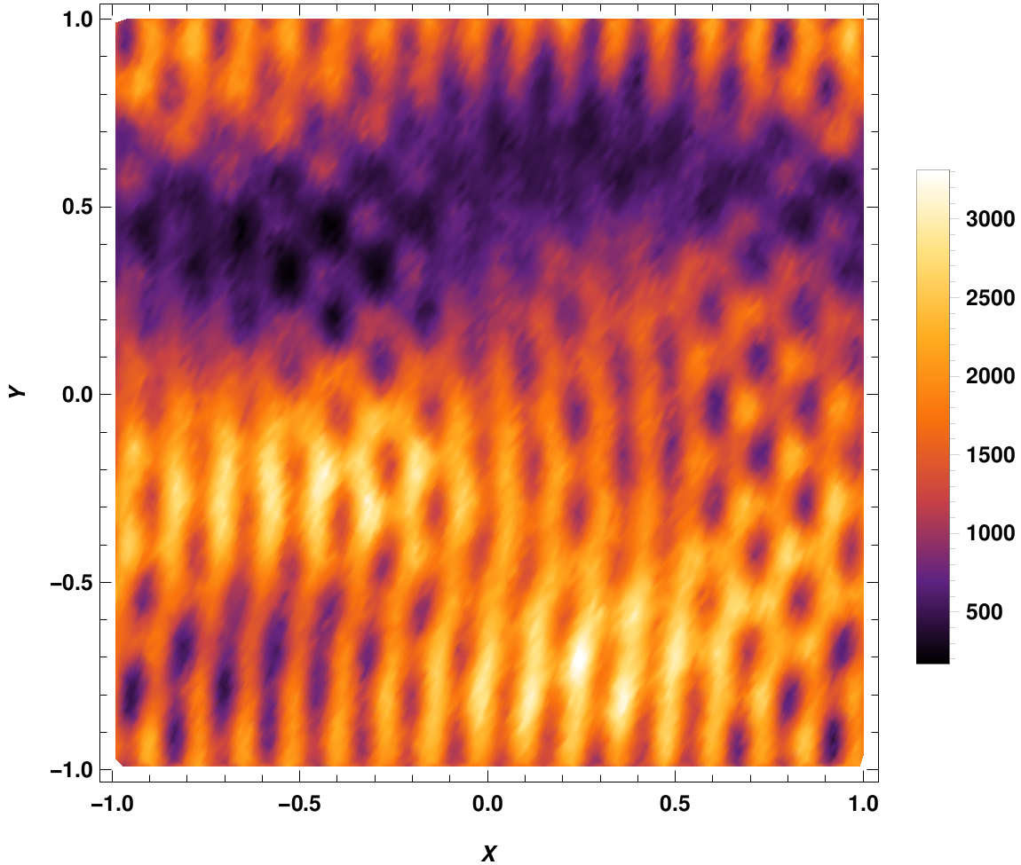
Figure 1: $\vec{E}^{2}$ at t=4$\Lambda^{-1}$ for initial configuration with random fluctuations

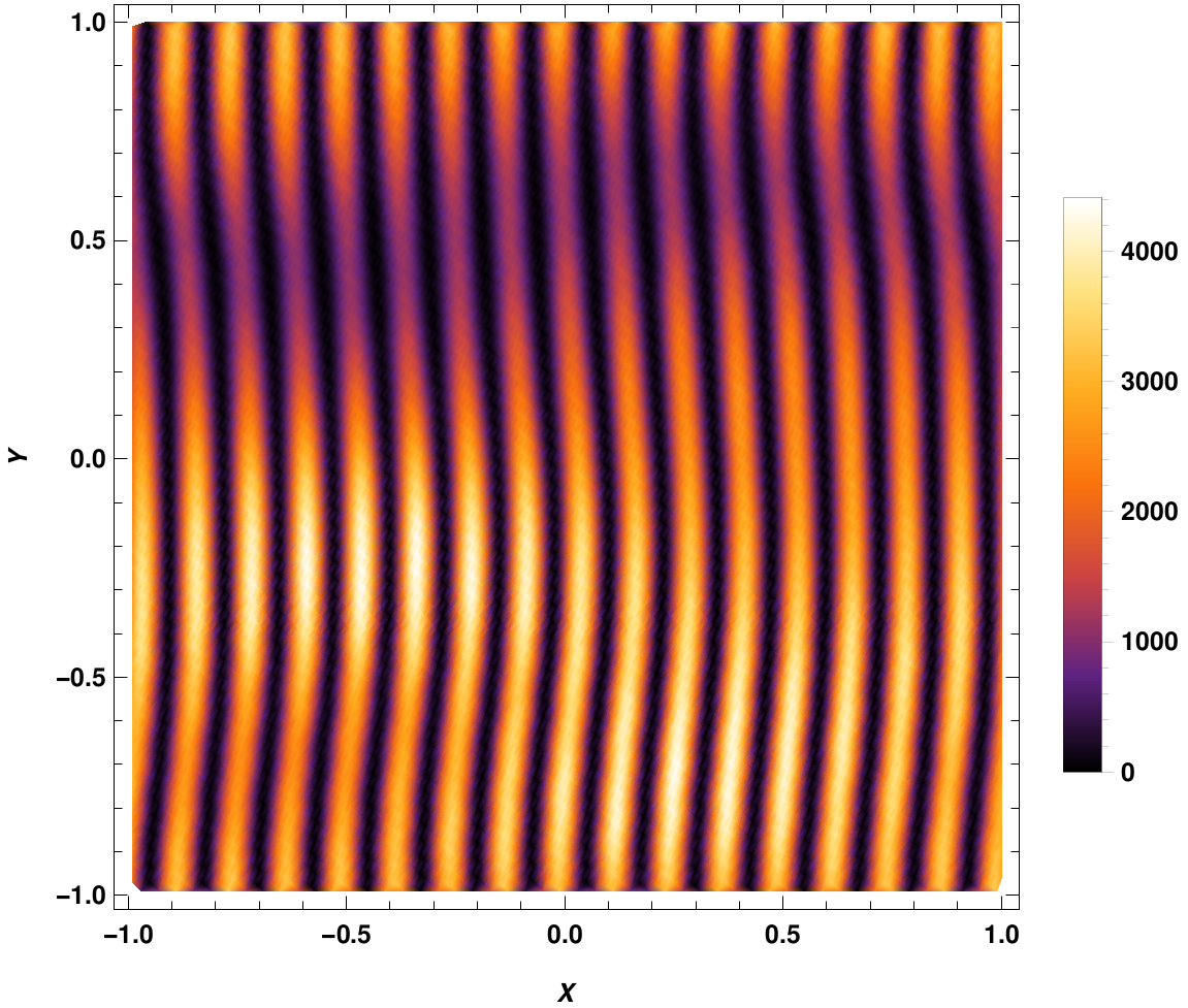
Figure 2: $\vec{B}^{2}$ at t=4$\Lambda^{-1}$ for initial configuration with random fluctuations

In Fig.2 and 2, $\rm{E}^{2}$ and ${\rm B}^{2}$ in units of $\Lambda^{4}$, respectively, are plotted at time $t=4\Lambda^{-1}$. It can be seen that within time interval $4\Lambda^{-1}$, these distributions have grown by about a factor of $O(10^{3})$.

In the case of non-abelian gauge fields, we compute the gauge invariant observables,

$${\rm E}^{2}_{SU(2)}=\sum_{i,a}F^{a,0i}F^{a,0i},{\rm B}^{2}_{SU(2)}=\sum_{a,i\neq j}F^{a,ij}F^{a,ij}$$ (16)

where spatial ($i,j$) and colour indices are summed over. The results for ${\rm E}^{2}_{SU(2)}$ and ${\rm B}^{2}_{SU(2)}$ at time $4\Lambda^{-1}$ are shown in Fig.4 and Fig.4. At initial time, the distributions of ${\rm E}^{2}_{SU(2)}$/${\rm B}^{2}_{SU(2)}$ are of the order of $O(10^{-1})\Lambda$/$O(1)\Lambda$. In time $4\Lambda^{-1}$ their distributions grow by a factor of $O(10^{4})$/$O(10^{3})$ respectively, due to parametric resonance.

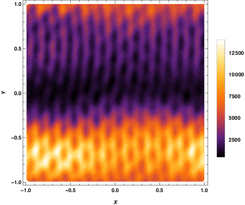
Figure 3: ${\rm E}^{2}_{SU(2)}$ at t=4$\Lambda^{-1}$ for initial configuration with random fluctuations

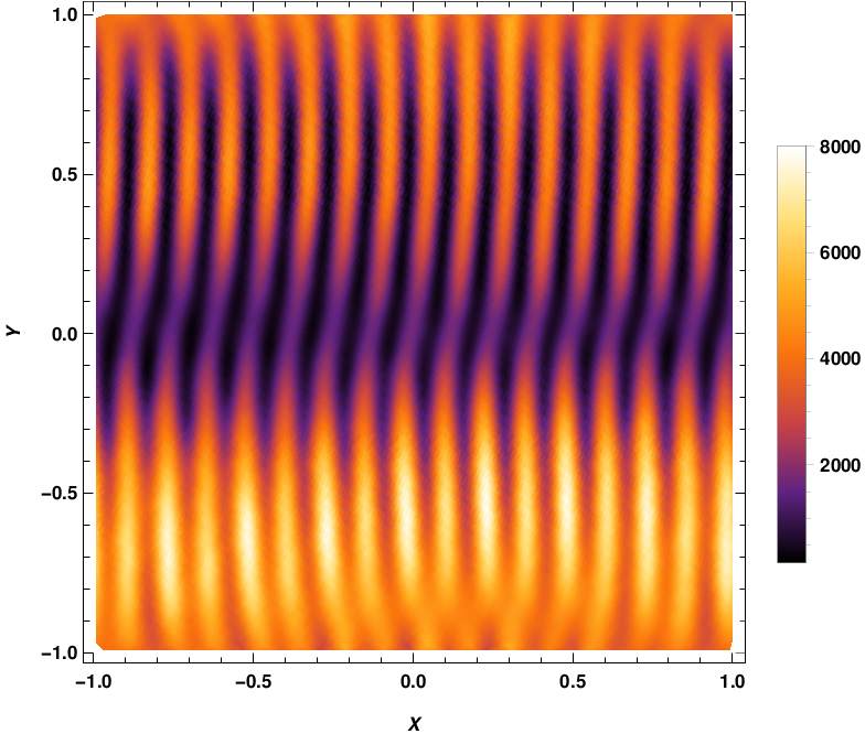
Figure 4: ${\rm B}^{2}_{SU(2)}$ at t=4$\Lambda^{-1}$ for initial configuration with random fluctuations

III.1 Parametric resonance, $U(1)$ vs $SU(2)$

To study the effect of interaction in $SU(2)$ gauge theory, we compute the spatial average of hamiltonian density, $\rho_{E}$ for $g=0,1$. The interactions between the gauge fields in $SU(2)$ significantly influence the growth of fluctuations. The self-interactions lead to a larger growth rate of fluctuations compared to the $U(1)\left(g=0\right)$ case for the same simulation parameters. To see this, we considered ten different random initial configurations. In the evolution of four of these, self-interaction resulted in higher growth of energy density at all times. For other configurations, the higher growth was observed only at later times. For example, in Fig.6, we have plotted $\rho_{E}$ for two such configurations. The non-linear interactions lead to higher growth only at late times. Up to $t=2.5\Lambda^{-1}$, the difference in $\rho_{E}$ between them is very small, $\left(<O(10^{-2})\right)$. The results are almost identical to the $U(1)$ gauge theory case, apart from the color factor. This is expected since the field fluctuations are initially small, and the field equations for $SU(2)$ gauge fields are almost identical to those in the $U(1)$ case, as the non-linear terms are negligible. Subsequently, however, with rapid growth in the fluctuations, the non-linear terms become significant. At this stage, the average energy density for $g=1$ and $g=0$ start to differ. In Fig.6, we have plotted $\Delta\rho_{E_{1-0}}=\rho_{E}(g=1)-\rho_{E}(g=0)$ of four initial random conditions for which $\Delta\rho_{E_{1-0}}$ is always positive after the initial fluctuations settle$\left(\approx t=1\Lambda^{-1}\right)$. We can see the difference goes on increasing exponentially with time. Similar to N-O instability, we observe increase in $\rho_{E}$ with increase in coupling constant. These results suggest that non-linear dynamics eventually enhances the growth of fluctuations. A detailed study of the power distribution in momentum space will provide a better understanding, which we plan to carry out in future.

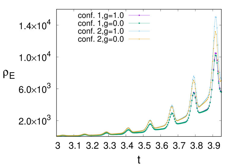
Figure 5: $\rho_{E}$ vs $t$ for $g=0$ and $g=1$.

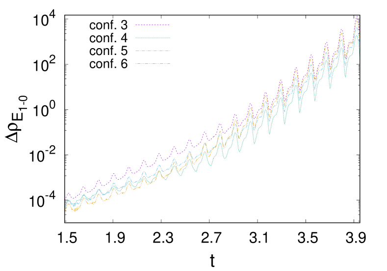
Figure 6: $\Delta\rho_{E_{1-0}}$ for random fluctuations.

To see that the parametric resonance results converge as the lattice space decrease, we evolve initial configurations with only one resonant mode along the ‘x’ direction, e.g; $k=8\pi\Lambda$ and $k=16\pi\Lambda$. The initial gauge fields are taken to be of the from $A^{a}_{\mu}=\delta sin(\kappa^{a}_{\mu}x)$ with space-time oscillation frequency $\omega=16\pi$. The results presented here are for $\kappa^{1}_{\mu}\equiv(\omega/2,\omega/2,\omega/2,\omega/2)$, $\kappa^{2}_{\mu}\equiv(-\omega/2,-\omega,\omega,0)$ and $\kappa^{3}_{\mu}\equiv(0,\omega,-\omega,-\omega/2)$. Note that $\kappa_{0}$ has nothing to do with temporal variations of the gauge field, but it represents the momentum mode of $A^{a}_{0}$ in ‘x’ direction. The conclusions drawn below will not change for other choices of configurations. This configuration satisfies the periodic boundary condition, i.e $A^{a}_{\mu}(x=0)=A^{a}_{\mu}(x=L)$, with $L=2\Lambda^{-1}$. For this choice of configuration, we do not see significant difference in energy density of $U(1)$ and $SU(2)$. The non-abelian evolution results in energy transfer bewteen differnt colors but not in overall increase of $\rho_{E}$. Higher value of coupling corresponds to higher transfer of energy between colors through modes. The effect of discretization is studied by considering suitable smaller lattice spacings. In the case of random initial conditions, it’s difficult to keep the amplitudes of momentum modes fixed while varying lattice spacing. For the above configuration, considering three different choices of lattice spacing, the evolutions of $\rho_{E}$ are shown in Fig.8 for $k_{x}=8\pi\Lambda$. Note that the energy density in $SU(2)$ case being smaller than $U(1)$ case for $\Delta x=0.0025\Lambda^{-1}$, may be due to the effect of over-damping. Above the time shown in Fig.8, numerical instabilities occur due to very large value of fields and their derivatives.

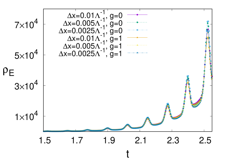
Figure 7: $\rho_{E}$ vs $t$ in continuum.

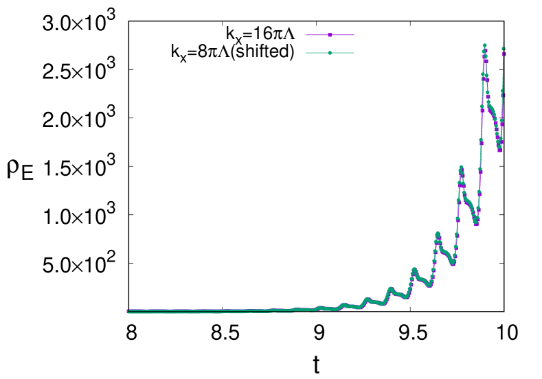
Figure 8: $\rho_{E}$ vs $t$ for $k_{x}=\omega$.

Now, considering only one color, i.e; abelian case, with all components being $k_{x}=8\pi$ and $k_{x}=16\pi$. The evolution of $\rho_{E}$ for $k_{x}=16\pi$ is shown in Fig.8. $\rho_{E}$ is small initially, up to $t\sim 8\Lambda^{-1}$, but subsequent evolution is similar to $k_{x}=8\pi$ case. For comparison, $\rho_{E}$ corresponding to $k_{x}=\omega/2$ is shifted in time(here by $\simeq 7.625\Lambda^{-1}$). This indicates that the $k_{x}=8\pi\Lambda$ mode is initially present, due to discretization of the $k_{x}=16\pi\Lambda$ mode. Though the amplitude is small, eventually, it dominates due to parametric resonance. This result suggests that the lowest resonant mode always dominates the evolution.

III.2 CP violations due to space-time oscillations

In the following, we present our results for the evolution of the distribution $\rho_{1}={\bf E}\cdot{\bf B}$ and $\rho_{2}={\bf E}^{a}\cdot{\bf B}^{a}$ in $U(1)$ and $SU(2)$ respectively. The initial value of $\rho_{1}$ is about $O(10^{-1})$. In Fig.10 and Fig.10, $\rho_{1}$ is shown at time $t=3\Lambda^{-1}$ and $t=4\Lambda^{-1}$. These figures show that over the lattice $\rho_{1}$ is distributed around zero. Within a time span of $\Lambda^{-1}$ the highest (lowest) value increase (decrease) by a factor of $\sim 20$.

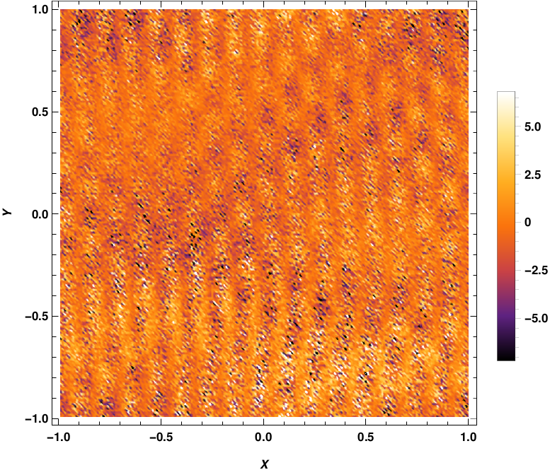
Figure 9: $\rho_{1}$ at $t=3\Lambda^{-1}$ for initial configuration with random fluctuations

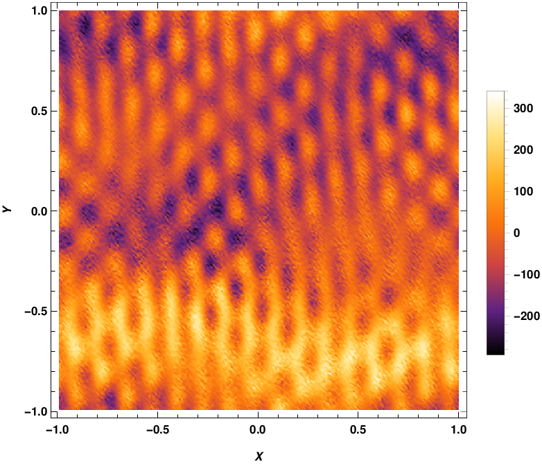
Figure 10: $\rho_{1}$ at $t=4\Lambda^{-1}$ for initial configuration with random fluctuations

The figures, Fig. 12 and Fig. 12, show $\rho_{2}$ at $t=3\Lambda^{-1}$ and $t=4\Lambda^{-1}$ respectively. Initially, the distribution of $\rho_{2}$ is within $[-0.5,0.5]\Lambda^{4}$. This range grows to $\sim[-17,18]\Lambda^{4}$ and $\sim[-1200,1300]\Lambda^{4}$, at $3\Lambda^{-1}$ and $4\Lambda^{-1}$ respectively.

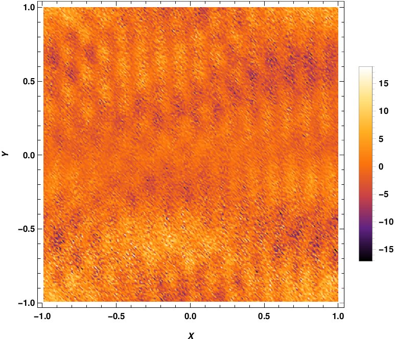
Figure 11: $\rho_{2}$ at $t=3\Lambda^{-1}$ for initial configuration with random fluctuations

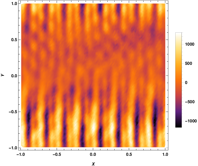
Figure 12: $\rho_{2}$ at $t=4\Lambda^{-1}$ for initial configuration with random fluctuations

The initial distribution of $\rho_{1}$ and $\rho_{2}$, in the above simulations, are non-zero. It is desirable to see results similar to the above with vanishing $\rho_{1}$ and $\rho_{2}$. An initial condition with vanishing $\rho_{1}$ and $\rho_{2}$ is difficult to achieve, with random fluctuations of the gauge fields. Thus, we considered gauge fields such that $\rho_{1}=0=\rho_{2}$, while the field strength tensors were non-zero in a localized region. Note that, the initial configuration needs to have non-zero (preferably resonant) modes, in order to couple to the space-time oscillations. Hence, we considered a gaussian form for the gauge fields for $U(1)$, i.e

$${\bf A}(t=0)=-\beta\Delta te^{-\alpha(x^{2}+y^{2})}\hat{k},A_{0}(t=0)=0;{\bf A}(t=\Delta t)=0,A_{0}(t=\Delta t)=0$$ (17)

$\alpha$ is taken to be the time period of one space-time oscillation. This makes sure that the initial configuration has non-zero resonant mode.

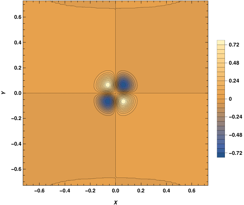
Figure 13: $\rho_{1}$ at $t=0.10\Lambda^{-1}$

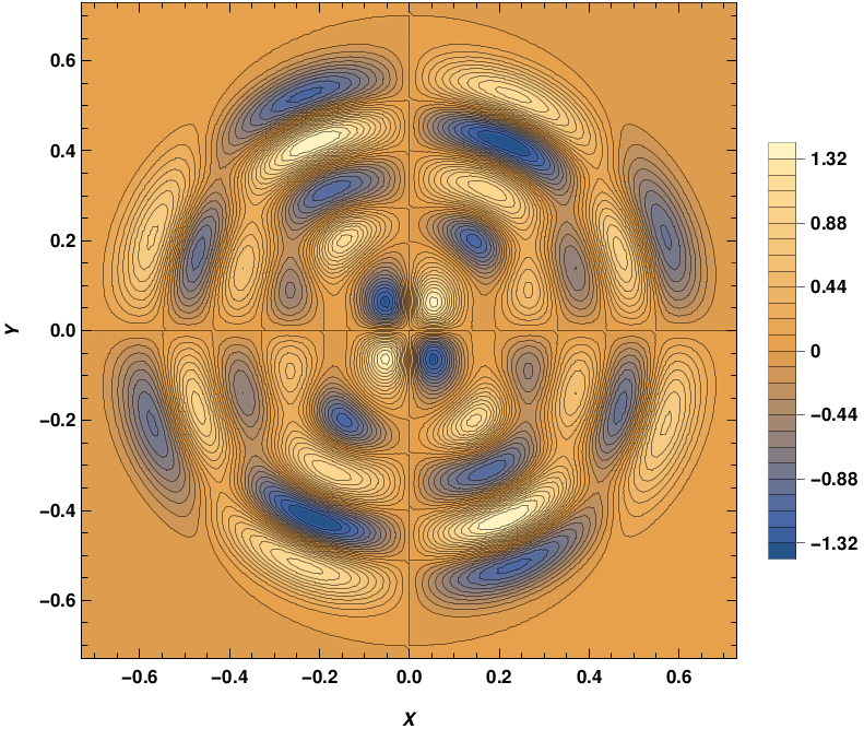
Figure 14: $\rho_{1}$ at $t=0.60\Lambda^{-1}$

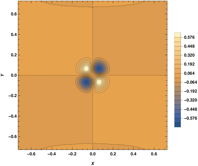
Figure 15: $\rho_{2}$ at $t=0.10\Lambda^{-1}$

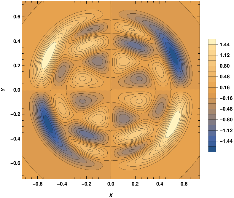
Figure 16: $\rho_{2}$ at $t=0.60\Lambda^{-1}$

For $SU(2)$ the gauge fields will have a colour index. When two of the three colour fields are zero, the evolution is always linear. Hence, we consider configurations for which the gauge fields are non-zero for at least two colours. Also, non-linear evolution requires that field strength and coupling constant should be large enough, e.g; here $\beta\Delta t\sim 0.1\Lambda$ and $g=1.5$. Note that even with smaller $\beta$ values the evolution will be non-linear at later times. The localized configurations, Eq.17, spread quickly during evolution. Once the fluctuations reach the boundary of the lattice, they lead to systematic errors in the evolution.

The figures, Fig.16 and Fig.16, show the distributions of $\rho_{1}$ at $t=0.10\Lambda^{-1}$ and $t=0.60\Lambda^{-1}$ respectively. The results for $\rho_{2}$ are shown in Fig.16 and 16 for $t=0.10\Lambda^{-1}$ and $t=0.60\Lambda^{-1}$ respectively. These results clearly show that $\rho_{1}$ and $\rho_{2}$ can take large values because of space-time oscillations. Further the effect of space-time oscillations is larger on $\rho_{2}$ due to non-linear interaction between the gauge fields. The volume average of $\rho_{2}$ ($<\rho_{2}>$), in $t=0.1\Lambda^{-1}$ to $t=0.6\Lambda^{-1}$, oscillates around zero and it’s amplitude increases by a factor of $O(10^{3})$. Hence, an overall increase in global CP violation is also observed. Note that the exponential increase in the CP both in $U(1)$ and $SU(2)$ will saturate due to the turbulent cascade mechanism studied in ref.Mace:2019cqo .

IV Discussion and conclusion

We have studied the evolution of abelian $U(1)$ as well as non-abelian $SU(2)$ gauge fields in the presence of space-time oscillations, using analytical as well as numerical simulations. The space-time oscillations frequency is taken to be $\omega$. Our results show that space-time oscillations induce parametric resonance in the modes of gauge fields. The modes, of the fields, undergoing parametric resonance are obtained from field equations for $U(1)$ and for $SU(2)$ in linear approximation in Fourier space. We also carry out numerical simulations in $2+1$ dimensions. These simulations are useful for studying the evolution of localized initial field configurations in $U(1)$. In the case of $SU(2)$ gauge fields, they are essential to study field dynamics beyond the linear regime. The numerical simulations also enable us to compare the dynamical evolution in the $U(1)$ and $SU(2)$ gauge theory.

In the process of the parametric resonance of the gauge field modes, large fluctuations of physical observables are generated. These observables include $F_{\mu\nu}\tilde{F}^{\mu\nu}$ and $F^{a}_{\mu\nu}\tilde{F}^{a\mu\nu}$ in $U(1)$ and $SU(2)$ gauge theory respectively, which break the $CP-$symmetry. Apart from the colour factor, the evolution of gauge fields is similar in both theories, when the fluctuations are small. At later times when the gauge field fluctuations grow, the effects of non-linear interactions in $SU(2)$ become important. The non-linear interactions drive larger growth in the fluctuations, beyond the conventional exponential growth expected in linear theories. The dynamics of the non-abelian gauge fields were found to be similar to that in the case of N-O instability due to chromo electric and magnetic fields. Our results also show that in the $U(1)/SU(2)$ case the dynamics of the evolution is dominated by the lowest resonant mode, i.e $k=\omega/2$ mode.

Our numerical simulations suggest that gravitational waves also will lead to parametric resonance in gauge fields. The gravitational waves will be dampened more efficiently due to the color factor. Further, the gravitational waves can induce large fluctuations in $CP$ violating physical observables. These observables can subsequently lead to a large-scale imbalance in local chiral charge distributions. Also a large non-zero ${\bf E}\cdot{\bf B}$ can enhance production of axions. The gravitational waves, in the early Universe also have the potential to generate large-scale magnetic fields, corresponding to resonant modes.

REFERENCES

References

- (1) L. Landau and E. M. Lifshitz, Mechanics (3rd Edition)(Elsevier, Oxford, 1976).
- (2) Osamu Ide, ‘Increased voltage phenomenon in a resonance circuit of unconventional magnetic configuration’, Journal of Applied Physics, 1995,77, 6015-6020.
- (3) L. A. Wu, H. J. Kimble, J. L. Hall and H. Wu, Phys. Rev. Lett. 57, 2520-2523 (1986) doi:10.1103/PhysRevLett.57.2520
- (4) D. G. Figueroa and F. Torrenti, JCAP 02, 001 (2017) doi:10.1088/1475-7516/2017/02/001 [arXiv:1609.05197 [astro-ph.CO]].
- (5) Araujo, G.C., Cabral, H.E., ‘Parametric Stability of a Charged Pendulum with an Oscillating Suspension Point’, Regul. Chaot. Dyn. 26, 39?60 (2021). https://doi.org/10.1134/S1560354721010032.
- (6) B. L. Hu and D. Pavon, “Intrinsic Measures of Field Entropy in Cosmological Particle Creation", Phys. Lett. B180, 329-334 (1986). doi:10.1016/0370-2693(86)91197-4
- (7) B. L. Hu and H. E. Kandrup, “Entropy Generation in Cosmological Particle Creation and Interactions: A Statistical Subdynamics Analysis", Phys. Rev. D 35, 1776-1792 (1987). doi:10.1103/PhysRevD.35.1776
- (8) H. E. Kandrup, “Entropy generation, particle creation, and quantum field theory in a cosmological spacetime: When do number and entropy increase?", Phys. Rev. D 37, 3505-3521 (1988). doi:10.1103/PhysRevD.37.3505
- (9) J. H. Traschen and R. H. Brandenberger, “Particle Production During Out-of-equilibrium Phase Transitions,” Phys. Rev. D 42, 2491-2504 (1990) doi:10.1103/PhysRevD.42.2491
- (10) L. Kofman, A. D. Linde and A. A. Starobinsky, “Reheating after inflation,” Phys. Rev. Lett. 73, 3195-3198 (1994) doi:10.1103/PhysRevLett.73.3195 [arXiv:hep-th/9405187 [hep-th]].
- (11) L. Kofman, A. D. Linde and A. A. Starobinsky, “Towards the theory of reheating after inflation,” Phys. Rev. D 56, 3258-3295 (1997) doi:10.1103/PhysRevD.56.3258 [arXiv:hep-ph/9704452 [hep-ph]].
- (12) J. P. Zibin, R. H. Brandenberger and D. Scott, Phys. Rev. D 63, 043511 (2001) doi:10.1103/PhysRevD.63.043511 [arXiv:hep-ph/0007219 [hep-ph]].
- (13) J. Jaeckel and S. Schenk, Phys. Rev. D 103, no.10, 103523 (2021) doi:10.1103/PhysRevD.103.103523 [arXiv:2102.08394 [hep-ph]].
- (14) C. Joana, Phys. Rev. D 106, no.2, 023504 (2022) doi:10.1103/PhysRevD.106.023504 [arXiv:2202.07604 [astro-ph.CO]].
- (15) D. Boyanovsky, H. J. de Vega, R. Holman, D. S. Lee and A. Singh, “Dissipation via particle production in scalar field theories,” Phys. Rev. D 51, 4419-4444 (1995). doi:10.1103/PhysRevD.51.4419 [arXiv:hep-ph/9408214 [hep-ph]].
- (16) S. Digal, R. Ray, S. Sengupta and A. M. Srivastava, “Resonant production of topological defects,” Phys. Rev. Lett. 84, 826-829 (2000) doi:10.1103/PhysRevLett.84.826 [arXiv:hep-ph/9911446 [hep-ph]].
- (17) E. A. L. Henn, J. A. Seman, G. Roati, K.M.F. Magalhes, and V. S. Bagnato, Phys. Rev. Lett. 103, 045301 (2009); E. A. L. Henn et al., Phys. Rev. A 79, 043618 (2009).
- (18) V.I. Yukalov, A.N. Novikov, and V.S. Bagnato, Phys. Lett. A 379, 1366 (2015).
- (19) V.I. Yukalov, E.P. Yukalova, and V.S. Bagnato, Phys. Rev. A 66, 043602 (2002).
- (20) M. Dvornikov, J. Phys. Conf. Ser. 1435, no.1, 012005 (2020) doi:10.1088/1742-6596/1435/1/012005 [arXiv:1910.01415 [hep-ph]].
- (21) M. Losada, Y. Nir, G. Perez, I. Savoray and Y. Shpilman, [arXiv:2205.09769 [hep-ph]].
- (22) D. Yoshida and J. Soda, PTEP 2018, no.4, 041E01 (2018) doi:10.1093/ptep/pty029 [arXiv:1710.09198 [hep-th]].
- (23) M. P. Hertzberg and E. D. Schiappacasse, JCAP 11, 004 (2018) doi:10.1088/1475-7516/2018/11/004 [arXiv:1805.00430 [hep-ph]].
- (24) A. Arza, T. Schwetz and E. Todarello, JCAP 10, 013 (2020) doi:10.1088/1475-7516/2020/10/013 [arXiv:2004.01669 [hep-ph]].
- (25) S. S. Dave and S. Digal, “Effects of oscillating spacetime metric background on a complex scalar field and formation of topological vortices,” Phys. Rev. D 103, 116007 (2021) doi:10.1103/PhysRevD.103.116007 [arXiv:1911.13216 [hep-th]].
- (26) S. S. Dave and S. Digal, “Field excitation in fuzzy dark matter near a strong gravitational wave source,” [arXiv:2106.05812 [gr-qc]].
- (27) B. P. Abbott et al.,‘GW170817: Observation of Gravitational Waves from a Binary Neutron Star Inspiral’, 2017a, PRL, 119, 161101, doi: 10.1103/PhysRevLett.119.161101
- (28) J. B. Griffiths, “Colliding Gravitational and Electromagnetic Waves,” Phys. Lett. A 54, 269-270 (1975) doi:10.1016/0375-9601(75)90254-6
- (29) J. Plebanski, Phys. Rev. 118, 1396-1408 (1959) doi:10.1103/PhysRev.118.1396
- (30) F. I. Cooperstock, “The Interaction Between Electromagnetic and Gravitational Waves,” Annals of Physics, 47 (1968), 173 doi:10.1016/0003-4916(68)90233-9
- (31) C. Barrabes and P. A. Hogan, “On The Interaction of Gravitational Waves with Magnetic and Electric Fields,” Phys. Rev. D 81, 064024 (2010) doi:10.1103/PhysRevD.81.064024 [arXiv:1003.0571 [gr-qc]].
- (32) Morozov, A.N., Pustovoit, V.I.,Fomin, I.V. ‘Generation of Gravitational Waves by a Standing Electromagnetic Wave’. Gravit. Cosmol. 27, 24?29 (2021), arXiv:2003.04104 [gr-qc], doi:10.1134/S020228932101014X.
- (33) W. Barreto, H. P. De Oliveira and E. L. Rodrigues, “Nonlinear interaction between electromagnetic and gravitational waves: an appraisal,” Int. J. Mod. Phys. D 26, no.12, 1743017 (2017) doi:10.1142/S0218271817430179 [arXiv:1705.05771 [gr-qc]].
- (34) T. Mishima and S. Tomizawa, [arXiv:2202.12060 [gr-qc]].
- (35) P. Jones, A. Gretarsson and D. Singleton, “Low frequency electromagnetic radiation from gravitational waves generated by neutron stars,” Phys. Rev. D 96, no.12, 124030 (2017) doi:10.1103/PhysRevD.96.124030 [arXiv:1709.09033 [gr-qc]].
- (36) W. Wang and Y. Xu, [arXiv:1811.01489 [gr-qc]].
- (37) H. Sotani, K. D. Kokkotas, P. Laguna and C. F. Sopuerta, Gen. Rel. Grav. 46, 1675 (2014) doi:10.1007/s10714-014-1675-5 [arXiv:1402.0251 [astro-ph.HE]].
- (38) P. Jones and D. Singleton, [arXiv:1907.08312 [gr-qc]].
- (39) A. Patel and A. Dasgupta, “Interaction of Electromagnetic field with a Gravitational wave in Minkowski and de-Sitter space-time,” [arXiv:2108.01788 [gr-qc]].
- (40) R. Brandenberger, P. C. M. Delgado, A. Ganz and C. Lin, [arXiv:2205.08767 [gr-qc]].
- (41) N. K. Nielsen and P. Olesen, Nucl. Phys. B 144, 376-396 (1978) doi:10.1016/0550-3213(78)90377-2
- (42) N. K. Nielsen and P. Olesen, Phys. Lett. B 79, 304 (1978) doi:10.1016/0370-2693(78)90249-6
- (43) S. Bazak and S. Mrowczynski, Phys. Rev. D 105, no.3, 034023 (2022) doi:10.1103/PhysRevD.105.034023 [arXiv:2111.11396 [hep-ph]].
- (44) S. J. Chang and N. Weiss, Phys. Rev. D 20, 869 (1979) doi:10.1103/PhysRevD.20.869
- (45) J. Berges, S. Scheffler, S. Schlichting and D. Sexty, Phys. Rev. D 85, 034507 (2012) doi:10.1103/PhysRevD.85.034507 [arXiv:1111.2751 [hep-ph]].
- (46) S. Tsutsui, H. Iida, T. Kunihiro and A. Ohnishi, Phys. Rev. D 91, no.7, 076003 (2015) doi:10.1103/PhysRevD.91.076003 [arXiv:1411.3809 [hep-ph]].
- (47) S. Tsutsui, T. Kunihiro and A. Ohnishi, Phys. Rev. D 94, no.1, 016001 (2016) doi:10.1103/PhysRevD.94.016001 [arXiv:1512.00155 [hep-ph]].
- (48) N. T. Bishop and L. Rezzolla, Living Rev. Rel. 19, 2 (2016) doi:10.1007/s41114-016-0001-9 [arXiv:1606.02532 [gr-qc]].
- (49) B. F. Schutz, ‘A first course in general relativity’, Cambridge University Press(1995).
- (50) W.H. Press, S.A. Teukolsky, W.T. Vetterling, and B.P. Flannery, Numerical Recipes in Fortran 77; The Art of Scientific Computing, 2nd ed. Vol. 1 (Syndicate, New York and Melbourne, 1997)
- (51) M. Mace, N. Mueller, S. Schlichting and S. Sharma, Phys. Rev. Lett. 124, no.19, 191604 (2020) doi:10.1103/PhysRevLett.124.191604 [arXiv:1910.01654 [hep-ph]].