Gradient Flow: Perturbative and Non-Perturbative Renormalization

Abstract

We review the gradient flow for gauge and fermion fields and its applications to lattice gauge theory computations. Using specific examples, we discuss the interplay between perturbative and non-perturbative calculations in the context of renormalization with the gradient flow.

1 Introduction

In the last decade a new tool, called the gradient flow (GF) Luscher:2010iy ; Luscher:2011bx ; Luscher:2013cpa , has earned its place as one of the most interesting development in lattice QCD calculations. The GF is a renormalizable ultraviolet smoothing procedure that modifies the short-distance behavior of fields. For lack of space it is not possible to review all the results obtained with the GF. The GF has a plethora of applications ranging from the definition of the topological charge density, the renormalization of gauge and fermion local fields, the running of the strong coupling and scale setting. We mainly discuss results and applications that pertain to the renormalization of local fields in lattice QCD and the interplay between perturbative and non-perturbative calculations. This is especially important for phenomenological applications. While the gradient flow has been defined and studied also for other field theories  Makino:2014sta ; Makino:2014cxa ; Suzuki:2015fka ; Hieda:2017sqq ; Kasai:2018koz , in these proceedings we only focus on SU($3$) gauge theories.

The GF for gauge fields appeared for the first time in Ref. Narayanan:2006rf in the study of Wilson loops for SU($N$) gauge theories at large $N$. It was noticed that modifying the gauge links in the loop with an APE smeared link projected to SU($N$), the naive continuum limit was equivalent to have continuum gauge fields satisfying what we now call the GF equation for gauge fields. In Ref. Luscher:2009eq the Wilson flow, a discretized version of the GF, was introduced as a gauge field transformation in the context of trivializing maps for gauge theories, and in Ref. Luscher:2010iy the GF was presented as a new tool to address a set of lattice gauge theories calculations. In particular it was shown Luscher:2010iy ; Luscher:2011bx that despite the apparent non-locality, correlation functions of flowed fields are still renormalizable to all orders in perturbation theory, and the renormalizability extends to include fermion fields Luscher:2013vga .

In the first part of these proceedings we discuss the GF for gauge fields and results related to the topological charge, the strong coupling and the scale setting. In the second part we present applications of the GF for fermions in the context of renormalization of local fields. We conclude with a survey of other results and final remarks.

2 Gradient flow for gauge fields

For gauge fields we consider the gradient flow defined by the following equation

$$\partial_{t}B_{\mu}(x,t)=D_{\nu}G_{\nu\mu}(x,t)\,,$$

$$\left.B_{\mu}(x,t)\right|_{t=0}=A_{\mu}(x)\,,$$ (1)

where $A_{\mu}$ is the non-abelian gluon field, $B_{\mu}$ denotes the flowed gluon field. The flowed field tensor is defined as the unflowed one $G_{\mu\nu}=\partial_{\mu}B_{\nu}-\partial_{\nu}B_{\mu}+\left[B_{\mu},B_{\nu}\right]$, and the flowed covariant derivative as $D_{\nu}=\partial_{\nu}+\left[B_{\nu},\cdot\right]$. It is immediate to notice that the flow time $t$ has energy dimension -2, thus the GF introduces a new length scale in the theory proportional to $\sqrt{t}$. The GF equation at vanishing strong coupling resembles a heat equation in $4$ dimensions and the solution is immediately found convoluting the heat kernel, $K(x,t)$ of the equation with the initial condition

$$B_{\mu}(x,t)=\int d^{4}y\leavevmode\nobreak\ K(x-y,t)A_{\mu}(y)\,,\quad K(x,t)=\int\frac{d^{4}p}{(2\pi)^{4}}{\textrm{e}}^{ipx}{\textrm{e}}^{-tp^{2}}=\frac{{\textrm{e}}^{-x^{2}/4t}}{(4\pi t)^{2}}\,.$$ (2)

The effect of the GF is to perform a Gaussian damping on the large momenta modes of the gauge fields, i.e. a smoothing a short distance over a range of $\sqrt{8t}$. A key property of the flowed gauge fields is that this tree-level result extends to all order in perturbation theory. Lüscher and Weisz have shown Luscher:2011bx that the flowed gauge fields in correlation functions do not require any additional renormalization beside the usual renormalization of the bare parameters of the theory.

The presence of the flow time does not complicate much perturbative calculations, and sophisticated technique already exists to extend the calculations to $2$-loops Artz:2019bpr and in same cases to $3$-loops Harlander:2016vzb . Numerically the GF can be integrated with infinitesimal "stout link smearing" steps Morningstar:2003gk , given the equivalence of the $2$ procedures.

2.1 Gradient flow and topological charge

The GF for gauge fields provides a renormalizable, and numerically easy to implement, definition of the topological charge $Q(t)=\int d^{4}x\leavevmode\nobreak\ q(x,t)$ with topological charge density

$$q(x,t)=\frac{1}{32\pi^{2}}\epsilon_{\mu\nu\rho\sigma}\textrm{Tr}\left\{G_{\mu\nu}(x,t)G_{\rho\sigma}(x,t)\right\}\,.$$ (3)

The r.h.s of the GF equation (1) can be written as the negative derivative of the Yang-Mills classical action (evaluated on flowed gauge fields) with respect to the field itself, i.e. $-\frac{\delta S_{\mathrm{YM}}(B)}{\delta B_{\mu}(x,t)}$. This implies that the GF equation naturally drives the fields towards the local minima of the theory Luscher:2010iy . This behavior can be observed in the left plot of Fig. 1, from Ref. Shindler:2015aqa , where it is shown the flow-time dependence of the topological charge evaluated on 2 representative SU($3$) Yang-Mills gauge configurations.

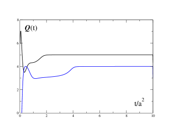
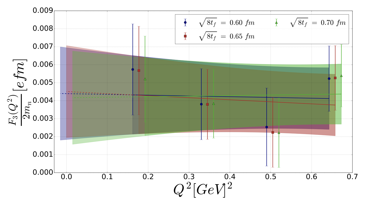
Figure 1: Left plot: Flow-time dependence of the topological charge on $2$ SU($3$) Yang-Mills gauge configurations. Right plot: Dependence of the nucleon CP-odd form factor on the momentum transfer $Q^{2}$ for a pion mass of $m_{\pi}\simeq 410$ MeV. The different colors correspond to the different flow times used to evaluate the topological charge.

We observe that after flowing to distances of $\sqrt{8t}\simeq 0.4-0.6$ fm the charge becomes independent of the flow time reaching a value very close to an integer. The property that the topological charge is independent of the flow time is a result of the topological nature of the observable Polyakov:1987ez ; Ce:2015qha ; Luscher:2021ygc . It can also be shown that this definition of the topological charge is equivalent to the fermionic definition based on Ginsparg-Wilson lattice Dirac operators in the Yang-Mills theory Ce:2015qha and in QCD Luscher:2021ygc . In conclusion the GF provides a computationally cheap and theoretically very robust definition of the topological charge.

There is one caveat related to the potential large O($a^{2}$) cutoff effects that this definition might have when evaluated on the lattice. Tree-level improvements Fodor:2014cpa , improved lattice definitions of the charge BilsonThompson:2002jk or improving flowed observables Ramos:2015baa following a more systematic Symanzik improvement program can help in performing the continuum limit.

In practice to define the topological charge in any correlation function it is sufficient to calculate it at flow times large enough as to avoid cutoff effects and not too large to avoid that the smoothing becomes too large and the correlators suffer from finite size effect. Fixing the flow time in physical units one can then perform the continuum limit. Examples are the calculation of the topological susceptibility of Refs. Bruno:2014ova ; Taniguchi:2016tjc .

2.2 Electric dipole moment from the $\theta$ term

The very attractive properties of the GF definition of the topological charge can be used to define other observables. One example is the electric dipole moment (EDM) induced by the $\theta$ term of QCD. In Euclidean space the theta term in the action is given by $i\overline{\theta}\int d^{4}x\leavevmode\nobreak\ \frac{1}{32\pi^{2}}\epsilon_{\mu\nu\rho\sigma}\textrm{Tr}\left\{G_{\mu\nu}(x)G_{\rho\sigma}(x)\right\}$. The EDM of a nucleon, $d_{\mathrm{N}}$, is proportional to the CP-odd form factor $F_{3}(Q^{2})$, $|d_{\mathrm{N}}|=F_{3}(Q^{2}=0)/2M_{\mathrm{N}}$, where $M_{\mathrm{N}}$ is the nucleon mass, parametrizing the $Q^{2}$ dependence of the matrix element

$$\left\langle N({\bf{p^{\prime}}},s^{\prime})|J_{\mu}^{\textrm{em}}|N({\bf{p}},s)\right\rangle=\overline{u}_{N}({\bf{p^{\prime}}},s^{\prime})\Gamma_{\mu}^{\bar{\theta}}(Q^{2})u_{N}({\bf{p}},s)\,,$$ (4)

evaluated in background where $\overline{\theta}\neq 0$, and where $\Gamma_{\mu}^{\bar{\theta}}(Q^{2})$ is decomposed in CP-even and CP-odd form factors. The Euclidean theory with $\overline{\theta}\neq 0$ has a complex action, thus one way to calculate the matrix element (4) is to evaluate the correlation function

$$\left\langle N(y_{0},{\bf{p_{2}}})J_{\mu}^{\mathrm{em}}(x_{0},{\bf{q}})\overline{N}(0,{\bf{p_{1}}})\right\rangle_{\overline{\theta}}$$ (5)

and expand in powers of $\overline{\theta}$. The nucleon EDM can then be determined calculating the 3-point function in Eq. (5) in a QCD background with the space-time insertion of the topological charge. The GF allows a definition of the nucleon EDM with no renormalization ambiguities, and contact terms are avoided due to the finite flow time. In the right plot of Fig. 1, from Ref. Dragos:2019oxn , we show the CP-odd form factor as a function of $Q^{2}$ and we observe that it is independent of the flow time for $\sqrt{8t}\simeq 0.6-0.7$ fm. One can then easily perform the continuum limit keeping the flow time fixed in physical units. The resulting neutron EDM Dragos:2019oxn is $|d_{n}|=0.00152(71)\overline{\theta}\leavevmode\nobreak\ e$ fm, which combined with the most recent experimental bounds provides the bound $|\overline{\theta}|<1.98\times 10^{-10}$ at the $90\%$ of confidence level. In Sec. 4 we will discuss another application of the GF applied to fermion fields that allow the calculation of other CP-violating contributions to the nucleon EDM.

2.3 Strong coupling

A very interesting application of the GF is the definition of the strong coupling Luscher:2010iy with the expectation value of the density

$$\left\langle E(t)\right\rangle=\left\langle\frac{1}{4}G_{\mu\nu}^{a}G_{\mu\nu}^{a}\right\rangle=3\frac{g_{0}^{2}}{\left(4\pi\right)^{2}t^{2}}+O(g_{0}^{4})\,.$$ (6)

From the leading order result we can use $E(t)$ to provide a non-perturbative definition of the coupling as

$$\overline{g}^{2}(\mu)=\left.\frac{16}{3}\pi^{2}t^{2}\left\langle E(t)\right\rangle\right|_{8t\mu^{2}=1}\,.$$ (7)

Asymptotic freedom implies that the short flow time behavior of $\left\langle E(t)\right\rangle$ can be described by perturbation theory. A perturbative expansion in $D=4-2\epsilon$ dimensions for a generic SU($N$) gauge theory results, for $N_{f}$ dynamical fermions, in

$$\left\langle E(t)\right\rangle=\frac{1}{2}g_{0}^{2}\frac{N^{2}-1}{(8\pi t)^{D/2}}(D-1)\left[1+c_{1}g_{0}^{2}+O(g_{0}^{4})\right]\,,$$ (8)

$$c_{1}=\frac{1}{16\pi^{2}}(4\pi)^{\epsilon}(8t)^{\epsilon}\left[N\left(\frac{11}{3}\frac{1}{\epsilon}+\frac{52}{9}-3\ln 3\right)-N_{f}\left(\frac{2}{3}\frac{1}{\epsilon}+\frac{4}{9}-\frac{4}{3}\ln 2\right)+O(\epsilon)\right]\,.$$ (9)

Renormalizing the bare coupling in the $\overline{\rm MS}$ removes completely the poles in Eq. (9), leading to the finite expression

$$\left\langle E\right\rangle=\frac{3}{4\pi t^{2}}\alpha(\mu)\left[1+k_{1}\alpha(\mu)+O(\alpha^{2})\right]\,,\qquad k_{1}=1.0978+0.0075\times N_{f}\,.$$ (10)

The strong coupling $\alpha(\mu)$ is now the renormalized coupling in the $\overline{\rm MS}$ scheme and Eq. (10) provides the connection with the flow-time dependence of $\left\langle E(t)\right\rangle$, i.e. the GF coupling defined in Eq. (7). This is the first example of the general result Luscher:2011bx we have described in Sec. 2, and it shows how to connect correlation functions computed with the GF to schemes that are more relevant for phenomenological applications. We will discuss in Sec. 3 more examples on how to connect flowed fields with fields at $t=0$ renormalized in the $\overline{\rm MS}$.

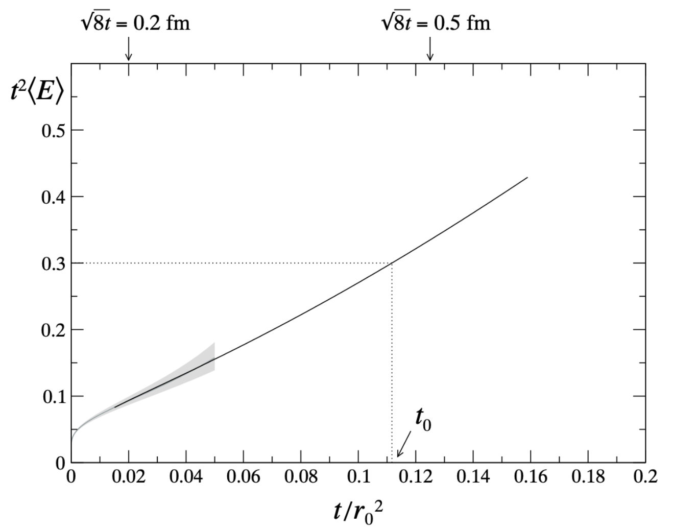
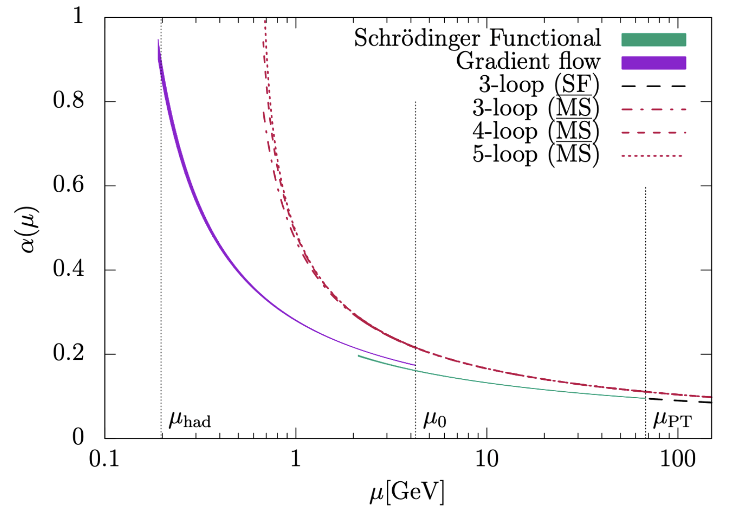
Figure 2: Left plot: Flow-time dependence of the energy $t^{2}\left\langle E(t)\right\rangle$ in the quenched model. The gray band is the prediction for perturbative QCD (see text) and $t_{0}$ denotes the flow time value where $t^{2}\left.\left\langle E(t)\right\rangle\right|_{t=t_{0}}=0.3$. Right plot: running coupling as a function of the renormalization scale for $3$ different schemes: the GF scheme described in the main text, the $\overline{\rm MS}$ scheme, and what is denoted as the Schrödinger functional scheme.

In the left plot of Fig. 2, from Ref. Luscher:2010iy , it is shown the flow-time dependence of $t^{2}\left\langle E\right\rangle$, solid black line, together with the perturbative estimate of Eq. (10) determined using the $4$-loop beta function in the $\overline{\rm MS}$ vanRitbergen:1997va . We observe a remarkable agreement between the perturbative estimate and the non-perturbative lattice data up to distances of $\sqrt{8t}\simeq 0.3$ fm corresponding to scales of $\sim 600$ MeV. In the region $\sqrt{8t}<0.2$ fm the lattice data are omitted because dominated by cutoff effects. This is a reflection of a well-known "window" problem encountered often in lattice QCD calculations. In this specific case the problem can be exemplified as follows. To properly match the perturbative calculation it is important to be at sufficiently short distances, but at the same time we cannot go at too small flow times otherwise lattice correlation functions will be dominated by cutoff effects. A well establish technique, finite size scaling Luscher:1991wu , provides a robust solution for this potential problem.

The calculation of the strong coupling using finite size scaling has a long history, and the scheme is usually dubbed as Schrödinger functional (SF) Luscher:1993gh ; Jansen:1995ck , because of the choice of boundary conditions in the "temporal" direction. For a review see Ref. Sommer:2006sj . Analogously to the infinite volume definition in Eq. (7), the GF coupling with SF boundary conditions Fritzsch:2013je can be defined in a small volume calculating the corresponding tree-level value of $\left\langle E(t)\right\rangle$ thus leading to

$$\overline{g}_{\mathrm{GF}}^{2}(L)=\left[\mathcal{N}^{-1}(c,T/L,x_{4}/T)\cdot t^{2}\left\langle E(t,x_{4})\right\rangle\right]_{t=c^{2}L^{2}/8}\,,$$ (11)

where $\mathcal{N}^{-1}(c,T/L,x_{4}/T)$ is the tree-level normalization factor depending on the temporal $T$ and spatial $L$ size of the box and on the time slice where $E(t,x_{4})$ is inserted. In the right plot of Fig. 2, taken from Ref. Bruno:2017gxd , is shown the running coupling as a function of the renormalization scale for $3$ different schemes: the GF scheme we just described, the $\overline{\rm MS}$ scheme, and what is denoted the Schrödinger functional scheme, where the same step-scaling procedure as in the GF scheme is adopted, but the coupling is defined from the response of a small variation of a specific background field. Technical details on the matching between the SF and the GF couplings can be found in Refs. DallaBrida:2016kgh ; Bruno:2017gxd . We just note that combining the GF and the SF couplings it is possible to cover a wide range of energies and that for the GF coupling there are indications DallaBrida:2019wur that is more difficult to make contact with perturbation theory than with the SF coupling, even at $3$-loop.

Other finite volume schemes have been used to define the strong coupling using for example periodic boundary conditions for the gauge fields and antiperiodic for fermions Fodor:2012td , twisted boundary conditions Ramos:2014kla or performing an infinite volume limit Hasenfratz:2019hpg .

2.4 Fixing the scale

To convert lattice QCD results obtained in lattice units, into dimensionful quantities, one needs to express the lattice spacing $a$ in physical units. This is achieved in hadronic renormalization schemes, using dimensionful experimentally measurable quantities.

The GF introduces a new scale, the flow time $t$, thus potentially providing a new relative way to fix the lattice spacing. Lüscher suggested Luscher:2010iy to use the density in Eq. 6 at hadronic distances to define the scale $t_{0}$ (see Fig. 2) by $\left.t^{2}\left\langle E(t)\right\rangle\right|_{t=t_{0}}=0.3$. The new scale $t_{0}$ can be then determined very precisely in the continuum limit in terms of the physical quantity of choice, and it has the advantage that does not need the analysis of correlation functions at large Euclidean times like for the determination of baryon masses. Even if not measurable experimentally $t_{0}$ allows to compare the continuum limit of completely independent calculations expressing all the lattice results in units of the appropriate power of $t_{0}$. Additionally once $t_{0}$ is determined very precisely in the continuum limit and in physical units, it can be used to renormalize other quantities retaining the same level of precision. A quantity related to $t_{0}$ has been introduced in Borsanyi:2012zs , dubbed $w_{0}$ which is fixed by the logarithmic derivative with respect to the flow time $t^{2}\left\langle E(t)\right\rangle$. The quark mass dependence of $t_{0}$ and $w_{0}$ is known from chiral perturbation theory Bar:2013ora . The largest lattice QCD collaborations have nowadays determined very precise values of $t_{0}$ and $w_{0}$ and they are summarized in FLAG review FlavourLatticeAveragingGroupFLAG:2021npn .

3 Gradient flow for fermions

Analogously as for gauge fields, it is possible to define a short distance smoothing operation also for fermion fields. The transformation is not unique, but we will focus on Lüscher’s proposal Luscher:2013cpa , where all the Dirac components are flowed in the same way. Alternative transformations have been discussed for example in Ref. Boers:2020lvc , but they dot seem to provide obvious advantages, neither numerically nor theoretically. The GF for fermions we consider is defined by

$$\partial_{t}\chi(x,t)=\Delta\chi(x,t)\qquad\partial_{t}\bar{\chi}(x,t)=\bar{\chi}(x,t)\overleftarrow{\Delta}$$ (12)

$$\chi(x,t=0)=\psi(x)\,,\quad\overline{\chi}(x,t=0)=\overline{\psi}(x)$$

where the laplacian $\Delta=D_{\mu}D_{\mu}$ is the squared of the flowed covariant derivative acting on the fundamental representation $D_{\mu}=\partial_{\mu}+B_{\mu}$. The gauge field $B_{\mu}$ has been flowed using the GF in Eq. (1).

As for the gauge fields a tree-level analysis immediately shows the smoothing properties of the GF over ranges of $\sqrt{8t}$. One important difference though is that the flowed fermion field requires renormalization Luscher:2013cpa , $\chi_{R}=Z_{\chi}^{-1/2}\chi$. The GF for fermions is still very powerful because any fermion local field, such as bilinears, 4-fermion or chromo-electric fields renormalize all multiplicatively with a renormalization factor depending only on the fermion content Luscher:2013cpa . If a local field ${\mathcal{O}}$ contains $n$ fermion and anti-fermion fields, the field will renormalize as ${\mathcal{O}}_{R}=Z_{\chi}^{-n/2}{\mathcal{O}}$. This is a consequence of the absence of short-distance singularities once we define the local field with an operator product expansion. A prime example of this phenomenon is the renormalization of the scalar density. In lattice QCD the scalar density $\overline{\psi}\psi$ mixes with lower dimensional operators generating $1/a^{3}$ power divergences, if the lattice action breaks chiral symmetry, or $1/a^{2}$ when using Ginsparg-Wilson fermions. The flowed scalar density $\Sigma(t)=\left\langle\overline{\chi}(t)\chi(t)\right\rangle$ instead renormalizes multiplicatively, i.e. $\Sigma_{R}(t)=Z_{\chi}^{-1}\Sigma(t)$. Considering how much the lattice community has struggled over power divergences, this result is quite remarkable and can be applied to many phenomenologically relevant flavor observables. Once the renormalization of the local fields is resolved, it remains to connect the renormalized matrix elements of flowed fields to the physical ones at $t=0$. The connection can be done in $2$ ways: using Ward identities Luscher:2013cpa ; DelDebbio:2013zaa ; Shindler:2013bia or relying on an operator product expansions at short flow time Luscher:2013vga , also called short flow-time expansion (SFtX).

Ward identities (WI) involving flowed fields are different from the standard WI. Using the modified modified chiral WI Luscher:2013cpa ; Shindler:2013bia and the spectral decomposition of pseudoscalar $P(x)$ 2-point functions it is possible to derive the following non-perturbative identity for the renormalized chiral condensate $\Sigma_{R}$

$$\Sigma_{R}=Z_{P}\lim_{m_{R}\rightarrow 0}\frac{G_{\pi}}{G_{\pi}(t)}\Sigma(t)\,,$$ (13)

where $G_{\pi}=\left\langle 0|P|\pi\right\rangle$ and $G_{\pi}(t)=\left\langle 0|P(t)|\pi\right\rangle$, while $\Sigma(t)=\left\langle\overline{\chi}(x,t)\chi(x,t)\right\rangle$. The problem of the power divergence is resolved and the condensate is calculable only knowing $Z_{P}$, $2$-point pseudoscalar densities and the flowed scalar expectation value. All these results are formally obtained in the continuum. At finite lattice spacing one should still make sure to avoid to use flow times too close to the values of the lattice spacing in use. After performing the continuum limit at fixed value of the flow time in physical units, the final result for $\Sigma_{R}$ should be flow-time independent.

3.1 Short flow-time expansion

It is not always possible to use WI to connect flowed renormalized fields, and the corresponding matrix elements, with the physical ones at $t=0$. It is possible though to use an OPE at small flow time, also known as short flow-time expansion (SFtX). The SFtX can be exemplified as follows. On the lattice we compute the correlation function of interest, where the local field ${\mathcal{O}}_{i,R}(t)$ is flowed and renormalized. The only renormalization needed is for the flowed fermion fields, beside the coupling and the quark mass. There are several ways to achieve this. One way is to use the following regularization independent and gauge invariant condition

$$\left\langle\mathring{\bar{\chi}}(x;t)\overleftrightarrow{\not{D}}\mathring{\chi}(x;t)\right\rangle=-\frac{2NN_{f}}{(4\pi)^{2}t^{2}}\,.$$ (14)

The $\mathring{\chi}$ and $\mathring{\bar{\chi}}$ are the so-called "ringed" fields Makino:2014wca ; Makino:2014taa which are now free from UV divergences. Another possibility would be to normalize the correlation functions with vector $2$-point functions Hasenfratz:2022wll . Independently of the method used the renormalization is greatly simplified, as there are no power divergences and no mixing with other fields, i.e. the renormalization is multiplicative.

Having renormalized the flowed fields one can use the SFtX

$$\mathcal{O}_{i,R}(t)\underset{t\rightarrow 0}{\sim}\sum_{i}c_{ij}(t,\mu)\mathcal{O}_{j,R}(t=0,\mu)\,,$$ (15)

to determine the target renormalized matrix element at $t=0$. The renormalization problem is now shifted to the determination of the matching coefficients $c_{ij}(t,\mu)$. The renormalized matrix elements $\mathcal{O}_{j,R}(t=0,\mu)$ are then determined in the same renormalization scheme used to determine the matching coefficients. When the SFtX receives contributions from lower dimensional operators the matching coefficients need to be determined non-perturbatively on the lattice Maiani:1991az ; Kim:2021qae ; Mereghetti:2021nkt . In Sec. 4 we discuss a method we have devised to determine non-perturbatively the matching coefficients of the power divergences. For contributions from fields of the same dimensions one can determine the matching coefficients directly in the continuum in perturbative QCD. This is a great simplification, compared with the original renormalization problem. Moreover the matching coefficients can be determined using standard techniques, where the SFtX is inserted in off-shell amputated and gauge-fixed 1PI correlation functions. The matching coefficients, after the renormalization procedure, will be independent on the gauge-fixing procedure and on the specific probes used to determine them.

4 Quark-chromo electric dipole moment

At hadronic scales BSM CP-violating sources for a non-vanishing EDM are encoded in higher-dimensional effective operators, containing the degrees of freedom of QCD and QED. One of these operators is the quark-chromo EDM (qCEDM)

$$\mathcal{O}_{\textrm{CE}}(x)=\sum_{f=u,d,s,\ldots}\overline{\psi}_{f}(x)\gamma_{5}\sigma_{\mu\nu}G^{a}_{\mu\nu}T^{a}\psi_{f}(x)\,.$$ (16)

In order to interpret future positive or null EDM experiments, and thus disentangle all possible CP-violating sources, it is important to determine renormalized qCEDM hadronic matrix elements using lattice QCD. The challenge of these type of calculations has been the very complicated renormalization pattern when using momentum-subtraction schemes Bhattacharya:2015rsa ; Cirigliano:2020msr . We have proposed Kim:2018rce ; Rizik:2020naq ; Kim:2021qae ; Mereghetti:2021nkt to use the GF to resolve the renormalization of the qCEDM and other CP-violating fields. We use the qCEDM as an example of the renormalization procedure using the SFtX we presented in the previous section.

For simplicity for now we consider the single flavor qCEDM. We now imagine that the flowed qCEDM has been defined with "ringed" fields, i.e. it has been renormalized,

$${\mathcal{O}}_{CE}^{R}(x;t)=\mathring{\bar{\chi}}(x;t)\sigma_{\mu\nu}G_{\mu\nu}(x;t)\mathring{\chi}(x;t)\,.$$ (17)

The leading contribution in the SFtX comes from the pseudoscalar density, that generates a power divergence. While in a typical lattice scheme this would be a power divergence in $1/a^{2}$ in the SFtX is a power divergence in $1/t$ and the coefficient, $c_{P}(t,\mu)$, should and can be determined non-perturbatively. In Ref. Kim:2021qae we have devised a gauge-invariant non-perturbative method to determine the matching coefficient that relies on the calculation of the ratio

$$\left[R_{P}(x_{4};t)\right]_{R}=t\frac{\left[\Gamma_{CP}(x_{4};t)\right]_{R}}{\left[\Gamma_{PP}(x_{4})\right]_{R}}\,,$$ (18)

$$\Gamma_{CP}(x_{4};t)=a^{3}\sum_{\bf{x}}\left\langle{\mathcal{O}}_{CE}^{ij}(x_{4},{\bf x};t)P^{ji}(0,{\bf 0};0)\right\rangle\,,\quad\Gamma_{PP}(x_{4})=a^{3}\sum_{{\bf x}}\left\langle P^{ij}(x_{4},{\bf x})P^{ji}(0,{\bf 0})\right\rangle\,.$$ (19)

Once we define the qCEDM in terms of the "ringed" fields and we renormalize the pseudoscalar density, the ratio (18) has a well defined continuum limit at fixed renormalized coupling and it can be used to determine the matching coefficient of the qCEDM into the pseudoscalar density, $c_{P}(t,\mu)$. In Ref. Kim:2021qae , we did not have at our disposal a complete determination of the "ringed" field, so we studied the dependence on the bare coupling of $c_{\chi}=tZ_{\chi}c_{P}(t,\mu)$, shown in the left plot of Fig. 3.

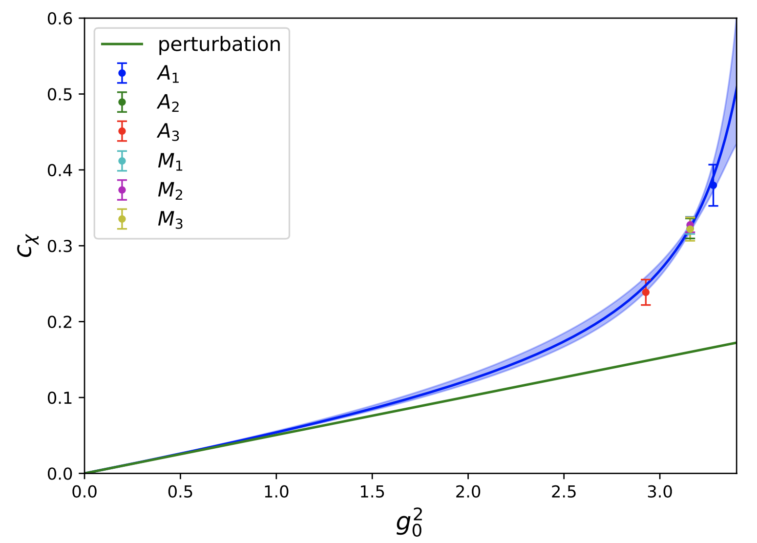
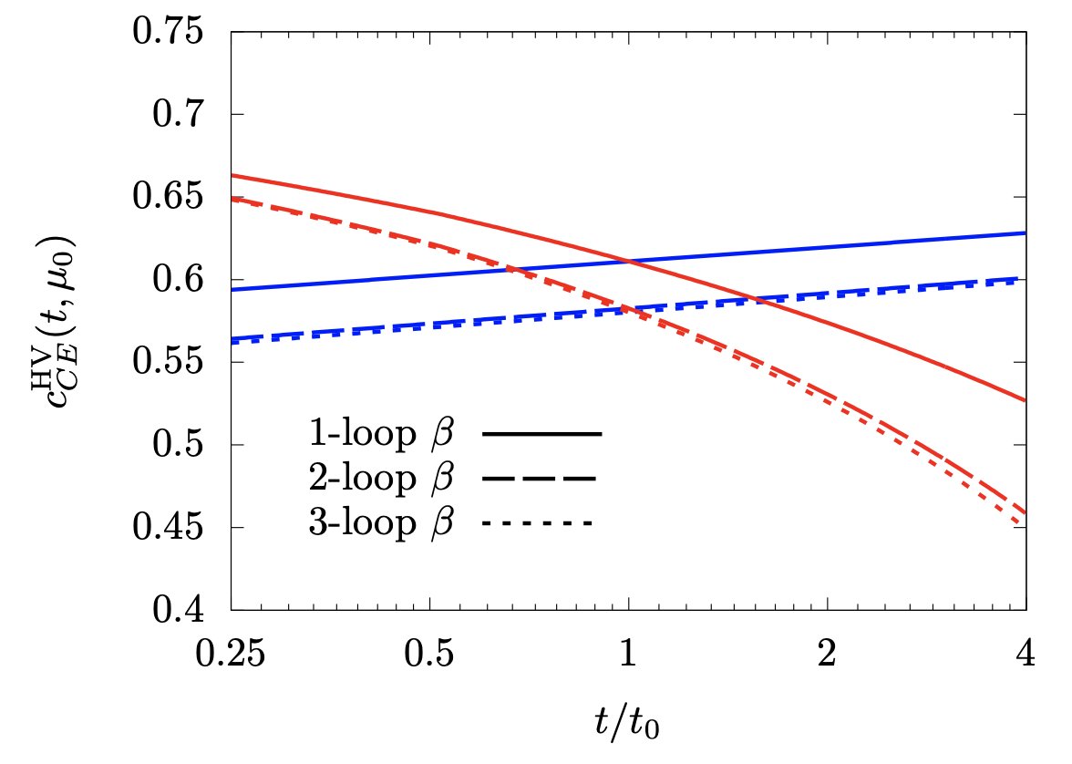
Figure 3: Left plot: bare coupling dependence of $c_{\chi}=tZ_{\chi}c_{P}(t,\mu)$. Lattice data with different colors (see Ref. Kim:2021qae ) are described with a Pade’ approximant constrained at small coupling by perturbation theory Rizik:2020naq . Right plot: scale dependence of the qCEDM matching coefficient. See main text and Ref. Mereghetti:2021nkt for details on the plot.

The colored data points represent lattice data at $3$ different lattice spacings and $3$ different pion masses (see Ref. Kim:2021qae for details) and the green line represents the first order perturbative result for $c_{P}(t,\mu)$ Rizik:2020naq . A Pade’ approximant, constraint with our perturbative result, describes well the data showing the relevance of a perturbative calculation of the matching coefficients, even for power divergences. In general the matching coefficient will depend on the scheme $S$ used to determine $Z_{P}^{(S)}$ and on the definition of "ringed" fields. When multiplied with the renormalized matrix element in the SFtX the dependence on the scheme $S$ will cancel out and the subtracted operator ${\mathcal{O}}_{\mathrm{sub}}(x;t)={\mathcal{O}}^{R}_{CE}(x;t)-c_{P}^{S}(t,\mu)P_{R}^{S}(x;\mu)$ will have a SFtX with contributions only from fields of the same or higher dimensions. To calculate the missing matching coefficients one can rely on perturbative QCD. We setup the theory in $D=4-2\epsilon$ dimensions and impose the following matching conditions on amputated 1PI correlation functions

$$Z_{\chi}^{-n/2}\left\langle\left(\psi\right)^{n_{\psi}}\left(\bar{\psi}\right)^{n_{\bar{\psi}}}\left(A_{\mu}\right)^{n_{A}}\mathcal{O}_{i}(t)\right\rangle^{\text{amp}}=c_{ij}(t,\mu)\,\left(Z_{jk}^{\text{MS}}\right)^{-1}\left\langle\left(\psi\right)^{n_{\psi}}\left(\bar{\psi}\right)^{n_{\bar{\psi}}}\left(A_{\mu}\right)^{n_{A}}{\mathcal{O}}_{k}\right\rangle^{\text{amp}}\,,$$ (20)

where $n$ is the total number of flowed fermion fields and the number of external fermion or gluon fields is chosen depending on what matching coefficient we want to isolate. The renormalized flowed fermion fields are given by

$$\chi_{R}(x;t)=(8\pi t)^{\varepsilon/2}\zeta_{\chi}^{1/2}\mathring{\chi}(x;t)\,,\quad\bar{\chi}_{R}(x;t)=(8\pi t)^{\varepsilon/2}\zeta_{\chi}^{1/2}\mathring{\bar{\chi}}(x;t)\,,$$ (21)

where $\zeta_{\chi}$ has been determined at 1-loop in Makino:2014taa ; Makino:2014wca and up to 2-loops in Refs. Harlander:2018zpi ; Artz:2019bpr .

The calculation of the matching coefficients can be summarized with the following steps. First renormalize the flowed fermion fields, e.g. using "ringed" fields, then expand in powers of external scales. The $t=0$ Feynman loop integrals vanish, being scaleless or, in other words, reflecting the cancellation between UV and IR poles. The $t>0$ Feynman loop integrals are only IR divergent and we regulate them in dimensional regularization. The resulting poles should match the UV poles in the $t=0$ side, thus can be removed with the renormalization needed at $t=0$. One is then left with a finite matching coefficient obtained in the same scheme used for the renormalization. In this way it is sufficient to just calculate the correlation functions containing the flow fields, expand in the external scale and then remove the IR divergences with the renormalization factors in the scheme we want to evaluate the matching coefficients. For full details of the calculation I refer to Ref. Mereghetti:2021nkt . As an example the matching coefficient of the qCEDM into itself is given by

$$c_{CE}(t,\mu)=\zeta_{\chi}^{-1}+\frac{\alpha_{s}}{4\pi}\left[2(C_{F}-C_{A})\log(8\pi\mu^{2}t)-\frac{1}{2}\Big{(}(4+5\delta_{\mathrm{HV}})C_{A}+(3-4\delta_{\mathrm{HV}})C_{F}\Big{)}\right]$$ (22)

where it is explicit the renormalization of the flowed fermion field with $\zeta_{\chi}$ and $\delta_{\mathrm{HV}}=0$ or $1$, whether we define $\gamma_{5}\sigma_{\mu\nu}$ in naive dimensional regularization or in the ’t Hooft-Veltman tHooft:1972tcz ; Breitenlohner:1977hr scheme. To estimate the uncertainty of the matching coefficient stemming from the truncation of the perturbative expansion we vary $c_{CE}(t,\mu)$ around the scale $t_{0}=\frac{1}{8\pi\mu_{0}^{2}}$ (not to be confused with $t_{0}$ discussed in Sec. 2.4) with $\mu_{0}=1.13$ GeV the scale in the MS scheme, corresponding to $\overline{\mu}_{0}=3$ GeV in the $\overline{\rm MS}$ scheme. In the right plot of Fig. 3 we show the scale dependence of $c_{CE}(t,\mu)$ in the t’Hooft-Veltman scheme where we keep the running coupling fixed at the scale $\mu_{0}$ (blue curves) or we vary it together with the matching coefficient (red curves). The spread of the curves, around $10-20\%$, gives us an indication of the uncertainty due to the truncation of the expansion. It is a rather strong indication that it would be beneficial to extend the calculation to $2-$loops and work in this direction is in progress.

5 Other applications

5.1 Finite temperature

In a hot QCD medium, transport coefficients characterize the motion of heavy quarks. They can be determined performing an heavy quark mass, $M$, expansion in $T/M$, where $T$ is the temperature. The first $2$ leading terms of the expansions can be estimated calculating 2-point static quarks correlation functions of chromo-electric and chromo-magnetic fields. Results for the momentum diffusion coefficient, $\kappa$, have been obtained using the GF Altenkort:2020fgs ; Brambilla:2022xbd . The main reason for the use of the GF for these type of calculations is to improve the signal-to-noise ratio especially at large Euclidean times. While these type of studies are still in their infancy, they can pave the way for a new application of the GF, especially because fields contributing to the heavy quark expansion need to be renormalized non-perturbatively.

5.2 Other results for fermion local fields

One of the important application of the GF is the renormalization of local fermion fields, like the qCEDM, as discussed in Secs. 3 and 4. The matching coefficients of fermion bilinears have been calculated for example in Refs. Hieda:2016lly . Other local fermion fields that can benefit from the GF are $4$-fermion operators. Perturbative calculations of the matching coefficients for the $4$-quark operators, relevant for $B_{K}$ and other contributions to the effective electroweak Hamiltonians, have been performed up to $2$-loops Suzuki:2020zue ; Harlander:2022tgk . The short-distance behavior of the product of $2$ fermion bilinears can be described by an OPE. The renormalization of the operators contributing to the OPE can be performed with the GF and the corresponding matching coefficients, up to and including $D=4$ fields have been calculated at $2$-loops in Ref. Harlander:2020duo .

5.3 Energy-momentum tensor

The renormalization of the energy-momentum tensor on the lattice is a rather non-trivial task. The trace of the tensor mixes with the identity and if we include fermions there is a mixing under renormalization between $5$ different dimension 4 fields. Using a SFtX, in refs. Suzuki:2013gza ; Makino:2014taa the matching coefficients in the pure gauge theory and with the inclusion of fermions have been determined. This method has been successfully tested numerically at finite temperature in the SU($3$) gauge theory in Ref. Kitazawa:2016dsl and with $N_{f}=2+1$ dynamical fermions in Taniguchi:2016ofw with $1-$loop matching, and in Ref. Taniguchi:2020mgg with a $2$-loop matching, using the perturbative calculation of Ref. Harlander:2018zpi . A different approach has been proposed in Ref. DelDebbio:2013zaa based on WI imposed to recover space-time symmetries at finite lattice spacing. It would be important to test numerically this approach.

5.4 Non-perturbative renormalization scheme

Even though the GF is not a renormalization group transformation, it can be used to define non-perturbative renormalization schemes. Attempts in this direction have started following different strategies in Refs. Monahan:2013lwa ; Hasenfratz:2022wll ; Battelli:2022kbe .

6 Conclusive remarks and acknowledgements

The gradient flow in recent years has played a prominent role in improving several aspects of lattice QCD calculations. It has provided a renormalizable definition of the topological charge, a new dimensionful scale to set the lattice spacing in physical units and an alternative definition of the strong coupling. It has also provided a new method to resolve challenges related to the renormalization of local fields, especially in the presence of power divergences and complicated mixing. Continuing to study all the nuances of the gradient flow, and extending the perturbative calculations of matching coefficients is a necessary step to address old and new challenges: e.g. in the non-perturbative studies of the CP-violating sources of the electric dipole moment, the effective electroweak Hamilonian and parton distribution functions.

I want to thank my collaborators N. Brambilla, A. Hasenfratz, R. Harlander, J. Kim, Z. Kordov, V. Leino, T. Luu, E. Mereghetti, C. Monahan, G. Pederiva, M. Rizik, P. Stoffer, A. Vairo, X. Wang, O. Witzel for many interesting discussions about the gradient flow and most enjoyable collaborations.

References

- (1) M. Lüscher, JHEP 1008, 071 (2010), 1006.4518
- (2) M. Lüscher, P. Weisz, JHEP 1102, 051 (2011), 1101.0963
- (3) M. Lüscher, JHEP 1304, 123 (2013), 1302.5246
- (4) H. Makino, H. Suzuki, PTEP 2015, 033B08 (2015), 1410.7538
- (5) H. Makino, F. Sugino, H. Suzuki, PTEP 2015, 043B07 (2015), 1412.8218
- (6) H. Suzuki, PTEP 2015, 043B04 (2015), 1501.04371
- (7) K. Hieda, A. Kasai, H. Makino, H. Suzuki, PTEP 2017, 063B03 (2017), 1703.04802
- (8) A. Kasai, O. Morikawa, H. Suzuki, PTEP 2018, 113B02 (2018), 1808.07300
- (9) R. Narayanan, H. Neuberger, JHEP 0603, 064 (2006), hep-th/0601210
- (10) M. Della Morte, A. Shindler, R. Sommer, JHEP 08, 051 (2005), hep-lat/0506008
- (11) M. Luscher, Commun. Math. Phys. 293, 899 (2010), 0907.5491
- (12) M. Lüscher, PoS LATTICE2013, 016 (2014), 1308.5598
- (13) J. Artz, R.V. Harlander, F. Lange, T. Neumann, M. Prausa, JHEP 06, 121 (2019), [Erratum: JHEP 10, 032 (2019)], 1905.00882
- (14) R.V. Harlander, T. Neumann, JHEP 06, 161 (2016), 1606.03756
- (15) C. Morningstar, M.J. Peardon, Phys. Rev. D 69, 054501 (2004), hep-lat/0311018
- (16) A. Shindler, T. Luu, J. de Vries, Phys. Rev. D 92, 094518 (2015), 1507.02343
- (17) A.M. Polyakov, Gauge Fields and Strings, Vol. 3 (1987)
- (18) M. Cè, C. Consonni, G.P. Engel, L. Giusti, Phys. Rev. D92, 074502 (2015), 1506.06052
- (19) M. Lüscher, Phys. Lett. B 823, 136725 (2021), 2109.07965
- (20) Z. Fodor, K. Holland, J. Kuti, S. Mondal, D. Nogradi, C.H. Wong, JHEP 09, 018 (2014), 1406.0827
- (21) S.O. Bilson-Thompson, D.B. Leinweber, A.G. Williams, Annals Phys. 304, 1 (2003), hep-lat/0203008
- (22) A. Ramos, S. Sint, Eur. Phys. J. C76, 15 (2016), 1508.05552
- (23) M. Bruno, S. Schaefer, R. Sommer (ALPHA), JHEP 08, 150 (2014), 1406.5363
- (24) Y. Taniguchi, K. Kanaya, H. Suzuki, T. Umeda, Phys. Rev. D 95, 054502 (2017), 1611.02411
- (25) C. Abel et al. (nEDM), Phys. Rev. Lett. 124, 081803 (2020), 2001.11966
- (26) J. Dragos, T. Luu, A. Shindler, J. de Vries, A. Yousif, Phys. Rev. C 103, 015202 (2021), 1902.03254
- (27) S. Capitani, M. Lüscher, R. Sommer, H. Wittig, Nucl. Phys. B 544, 669 (1999), [Erratum: Nucl.Phys.B 582, 762–762 (2000)], hep-lat/9810063
- (28) T. van Ritbergen, J.A.M. Vermaseren, S.A. Larin, Phys. Lett. B 400, 379 (1997), hep-ph/9701390
- (29) M. Luscher, P. Weisz, U. Wolff, Nucl. Phys. B 359, 221 (1991)
- (30) M. Luscher, R. Sommer, P. Weisz, U. Wolff, Nucl. Phys. B 413, 481 (1994), hep-lat/9309005
- (31) K. Jansen, C. Liu, M. Luscher, H. Simma, S. Sint, R. Sommer, P. Weisz, U. Wolff, Phys. Lett. B 372, 275 (1996), hep-lat/9512009
- (32) R. Sommer, Non-perturbative QCD: Renormalization, O(a)-improvement and matching to Heavy Quark Effective Theory, in Workshop on Perspectives in Lattice QCD (2006), hep-lat/0611020
- (33) P. Fritzsch, A. Ramos, JHEP 10, 008 (2013), 1301.4388
- (34) M. Bruno, M. Dalla Brida, P. Fritzsch, T. Korzec, A. Ramos, S. Schaefer, H. Simma, S. Sint, R. Sommer (ALPHA), Phys. Rev. Lett. 119, 102001 (2017), 1706.03821
- (35) M. Dalla Brida, P. Fritzsch, T. Korzec, A. Ramos, S. Sint, R. Sommer (ALPHA), Phys. Rev. D95, 014507 (2017), 1607.06423
- (36) M. Dalla Brida, A. Ramos, Eur. Phys. J. C79, 720 (2019), 1905.05147
- (37) Z. Fodor, K. Holland, J. Kuti, D. Nogradi, C.H. Wong, JHEP 1211, 007 (2012), 1208.1051
- (38) A. Ramos, JHEP 11, 101 (2014), 1409.1445
- (39) A. Hasenfratz, O. Witzel, Phys. Rev. D 101, 034514 (2020), 1910.06408
- (40) S. Borsanyi, S. Durr, Z. Fodor, C. Hoelbling, S.D. Katz et al., JHEP 1209, 010 (2012), 1203.4469
- (41) O. Bar, M. Golterman, Phys. Rev. D 89, 034505 (2014), [Erratum: Phys.Rev.D 89, 099905 (2014)], 1312.4999
- (42) Y. Aoki et al. (Flavour Lattice Averaging Group (FLAG)), Eur. Phys. J. C 82, 869 (2022), 2111.09849
- (43) M. Boers, JHEP 01, 204 (2021), 2011.05316
- (44) L. Del Debbio, A. Patella, A. Rago, JHEP 11, 212 (2013), 1306.1173
- (45) A. Shindler, Nucl. Phys. B 881, 71 (2014), 1312.4908
- (46) H. Makino, H. Suzuki (2014), 1404.2758
- (47) H. Makino, H. Suzuki, PTEP 2014, 063B02 (2014), 1403.4772
- (48) A. Hasenfratz, C.J. Monahan, M.D. Rizik, A. Shindler, O. Witzel, PoS LATTICE2021, 155 (2022), 2201.09740
- (49) L. Maiani, G. Martinelli, C.T. Sachrajda, Nucl. Phys. B 368, 281 (1992)
- (50) J. Kim, T. Luu, M.D. Rizik, A. Shindler (SymLat), Phys. Rev. D 104, 074516 (2021), 2106.07633
- (51) E. Mereghetti, C.J. Monahan, M.D. Rizik, A. Shindler, P. Stoffer, JHEP 04, 050 (2022), 2111.11449
- (52) T. Bhattacharya, V. Cirigliano, R. Gupta, E. Mereghetti, B. Yoon, Phys. Rev. D 92, 114026 (2015), 1502.07325
- (53) V. Cirigliano, E. Mereghetti, P. Stoffer, JHEP 09, 094 (2020), 2004.03576
- (54) J. Kim, J. Dragos, A. Shindler, T. Luu, J. de Vries, in 36th International Symposium on Lattice Field Theory (Lattice 2018) East Lansing, MI, United States, July 22-28, 2018 (2018), 1810.10301
- (55) M.D. Rizik, C.J. Monahan, A. Shindler (SymLat), Phys. Rev. D 102, 034509 (2020), 2005.04199
- (56) T. Izubuchi, H. Ohki, S. Syritsyn, in 37th International Symposium on Lattice Field Theory (2020), 2004.10449
- (57) R.V. Harlander, Y. Kluth, F. Lange, Eur. Phys. J. C 78, 944 (2018), [Erratum: Eur.Phys.J.C 79, 858 (2019)], 1808.09837
- (58) G. ’t Hooft, M. Veltman, Nucl. Phys. B 44, 189 (1972)
- (59) P. Breitenlohner, D. Maison, Commun. Math. Phys. 52, 11 (1977)
- (60) L. Altenkort, A.M. Eller, O. Kaczmarek, L. Mazur, G.D. Moore, H.T. Shu, Phys. Rev. D 103, 014511 (2021), 2009.13553
- (61) N. Brambilla, V. Leino, J. Mayer-Steudte, P. Petreczky (TUMQCD) (2022), 2206.02861
- (62) K. Hieda, H. Suzuki, Mod. Phys. Lett. A 31, 1650214 (2016), 1606.04193
- (63) A. Suzuki, Y. Taniguchi, H. Suzuki, K. Kanaya, Phys. Rev. D 102, 034508 (2020), 2006.06999
- (64) R.V. Harlander, F. Lange, Phys. Rev. D 105, L071504 (2022), 2201.08618
- (65) R.V. Harlander, F. Lange, T. Neumann, JHEP 08, 109 (2020), 2007.01057
- (66) H. Suzuki, PTEP 2013, 083B03 (2013), 1304.0533
- (67) M. Kitazawa, T. Iritani, M. Asakawa, T. Hatsuda, H. Suzuki, Phys. Rev. D94, 114512 (2016), 1610.07810
- (68) Y. Taniguchi, S. Ejiri, R. Iwami, K. Kanaya, M. Kitazawa, H. Suzuki, T. Umeda, N. Wakabayashi, Phys. Rev. D96, 014509 (2017), [Erratum: Phys. Rev.D99,no.5,059904(2019)], 1609.01417
- (69) Y. Taniguchi, S. Ejiri, K. Kanaya, M. Kitazawa, H. Suzuki, T. Umeda (WHOT-QCD), Phys. Rev. D 102, 014510 (2020), [Erratum: Phys.Rev.D 102, 059903 (2020)], 2005.00251
- (70) C. Monahan, K. Orginos, PoS Lattice2013, 443 (2014), 1311.2310
- (71) N. Battelli, S. Sint, PoS LATTICE2021, 437 (2022)