Boosting Synthetic Data Generation with Effective Nonlinear Causal Discovery

Abstract

Synthetic data generation has been widely adopted in software testing, data privacy, imbalanced learning, artificial intelligence explanation, etc. In all such contexts, it is important to generate plausible data samples. A common assumption of approaches widely used for data generation is the independence of the features. However, typically, the variables of a dataset depend on one another, and these dependencies are not considered in data generation leading to the creation of implausible records. The main problem is that dependencies among variables are typically unknown. In this paper, we design a synthetic dataset generator for tabular data that is able to discover nonlinear causalities among the variables and use them at generation time. State-of-the-art methods for nonlinear causal discovery are typically inefficient. We boost them by restricting the causal discovery among the features appearing in the frequent patterns efficiently retrieved by a pattern mining algorithm. To validate our proposal, we design a framework for generating synthetic datasets with known causalities. Wide experimentation on many synthetic datasets and real datasets with known causalities shows the effectiveness of the proposed method.

I Introduction

In many real-world applications, it is fundamental to rely on synthetic data, especially when real data can be difficult to obtain due to privacy issues, temporal or budget constraints, or the unavailability of large quantities. Synthetic data are used for validating data discovery applications and for testing software in a controlled environment that satisfies specific conditions [1, 2]. In machine learning, synthetic data are increasingly being used for addressing imbalanced learning [3], for training a model with the intention of transfer learning to real data [4], or, in the last days, for providing explanations of obscure decision systems [5]. Indeed, various studies show the benefits of using synthetic data located in the neighborhood of available real instances for learning predictive models [6, 7], or for explaining the reasons for the prediction [8].

In these scenarios, the methods used for synthetic data generation are either simple but efficient random approaches assuming uniform distribution for all the variables [5], or complex and time expensive methods such as Generative Adversarial Networks (GAN) [9]. However, typically, only a few of them rely on explicit knowledge about possible linear and/or nonlinear dependencies among the variables. In particular, common generative approaches work on the assumption that the variables of the dataset to generate are independent. Such an assumption does not guarantee a reliable synthetic generation of the dataset under analysis. On the other hand, GAN-like approaches can theoretically learn possible dependencies, but these are not explicitly represented, and there is no guarantee that they are followed in the data generation process.

Therefore, a crucial problem in synthetic data generation is that dependencies among variables are not used because they are typically unknown. Our idea is to design a technique for synthetic data generation that accounts for dependencies among variables by exploiting a causal discovery algorithm. Causal discovery algorithms take as input a set of variables belonging to a dataset and determine which are the causal relationships among them [10, 11]. In particular, we focus on nonlinear causal discovery [12]. If the dataset under analysis is continuous-valued, methods based on linear causal models are commonly applied [13]. This typically happens because linear models are well understood and not necessarily because the true causal relationships are believed to be linear [12]. However, in reality, many causal relationships are nonlinear, raising doubts on the reliability and usability of linear methods. In addition, in [12] it is shown that considering nonlinear causal relationships plays a primary role in the identification of causal directions. For these reasons, we start from the nonlinear causal discovery method described in [12] (ncd) to design our synthetic data generator exploiting causal relationships. Besides non-linearity, the ncd is able to consider and discover not only binary relationships but also multivariate ones. Unfortunately, the ncd approach is inefficient and can only be employed to reveal the causal relationships of datasets with a very small number of variables. Thus, it is not practically usable for applications on real datasets. Our proposal is to boost ncd by restricting the search of causalities among the features appearing in the patterns returned by a pattern mining algorithm executed on the same dataset.

Our contribution is twofold. First, we design an efficient method for nonlinear causal discovery based on pattern mining named ncda (nonlinear causal discovery with Apriori). Second, we implement gencda, a generative method based on ncda. Moreover, to validate our proposal, we realized a framework for generating synthetic datasets with known causalities. We report wide experimentation on synthetic datasets and real datasets with known causalities highlighting the effectiveness of our proposals both in terms of time and accuracy for causal discovery and data generation.

The rest of the paper is organized as follows. Section II discusses related works. Section III recalls the notions needed to understand the proposed methods which are illustrated in Section IV. Section V presents the experimental results. Finally, Section VI concludes the paper by discussing known limitations and proposing future research directions.

II Related Works

In this section, we review existing proposals in the literature related to causal discovery and synthetic data generation.

The discovery of causal relationships between a set of observed variables is a fundamental problem in science because it enables predictions of the consequences of actions [13]. Thus, the development of automatic and data-driven causal discovery methods constitutes an important research topic [13, 14, 15]. A standard approach for causal discovery is to estimate a Markov equivalence class of directed acyclic graphs from the data [13, 14]. The independence tests often adopt linear models with Gaussian noise [14]. However, [16] shows that non-Gaussian noise in linear models can actually help in distinguishing the causal directions. In [12, 17, 18] is shown that nonlinear models can play a role similar to that of non-Gaussianity. Indeed, when causal relationships are nonlinear it allows the identification of causal directions by breaking the symmetry between the variables. Also, [19] shows that non-invertible functional relationships between the variables can provide clues to identify causal relationships. For nonlinear models with additive noise almost any nonlinear relationship (invertible or not) typically suggests identifiable models. In [17] is presented a nonlinear causal discovery approach for high dimensional data based on the idea of mapping the observations to high dimensional space with a kernel such that the nonlinear relations become simple linear ones. A problem of the aforementioned nonlinear causal discovery approaches is that they can miss detecting indirect causal relationships, which are frequently encountered in practice and result from omitted intermediate causal variables. In [18] is proposed a cascade nonlinear additive noise model to represent such causal influences in a way that each direct causal relation follows the nonlinear additive noise model only observing initial cause and final effect. Despite various advantages of the recent proposals, to the best of our knowledge, the nonlinear causal discovery described in [12] is the only one that allows managing not only binary relationships. For this reason, we adopt it as starting point of our procedure. However, we highlight that our proposal is a framework that can exploit the preferred causal discovery method.

The need to generate synthetic data derives from the first data imputation work to solve the problem of non-responses in statistical surveys [20]. In [21] is described one of the first multiple imputation techniques used to synthetically generate the values of a set of missing attributes for the records of the dataset. In [22] are implemented and extend multiple imputation approaches for the specific case of synthetic data generation. In machine learning, synthetic data are often used for handling the classification task in case of imbalanced data and for addressing the problem of outcome explanation of black-box classifiers. Concerning imbalanced learning, the smote algorithm [3] generates an arbitrary number of synthetic instances to shift the learning bias toward the minority class. The adasyn approach [23] is based on the idea of adaptively generating minority data samples according to their distributions. In practice, the method generates more synthetic samples for minority classes that are harder to learn compared to those minority samples that are easier to learn. In [24] is introduced an alternative method to synthesize data through a non-parametric technique that uses classification and regression trees. In [25] is proposed DataSynthesizer, a technique that captures the underlying correlation structure between different attributes by building a Bayesian network. Another recent generator is the Synthetic Data Vault (sdv) [26] which uses the multivariate Gaussian copula (gcm) to calculate the covariances between the input columns. After that, the distributions and covariances are sampled to return synthetic data. In addition, recently, many generative models have been developed based on Generative Adversarial Networks (GANs) and their extensions [9] and autoencoders [27]. Their success is due to their high effectiveness and flexibility in generating and representing data. These approaches are particularly employed for the generation of synthetic images and, in general, for unstructured data such as text or time series. However, recently, they are being effectively applied also for the generation of tabular data. In [28] and [29] are proposed synthetic tabular data generators using GANs, Conditional GANs and Variational Autoencoders (VAE). Unfortunately, since they are based on deep learning procedures, they require a non-negligible amount of data and a considerable amount of time. Finally, in eXplainable Artificial Intelligence (XAI) [8], data generation approaches are used to learn interpretable models able to mimic black-box decision systems. lime [5] explains the local behavior of a black-box classifier by learning a linear model on synthetic data generated around the instance to explain using a normal distribution. lore [30] is another local explanation method that exploits a synthetic neighborhood generation based on a genetic algorithm to create a more compact dataset around the explained instance.

Among wide literature concerning synthetic data generation and causality, integrated approaches are a recently challenging research area. In [31], authors implement CauseMe, a platform to benchmark causal discovery methods acting on time series. In 2021, Lawrence et al. [32] propose an easily parameterizable process that provides the capability to generate synthetic time series from vastly different scenarios. Lastly, Wood-Doughty et al. [33] present a synthetic text generator to evaluate causal inference (not causal discovery) methods. Thus, to the best of my knowledge, no state-of-the-art synthetic data generators explicitly allow for encoding causal relationships.

III Setting the Stage

In this paper, we address the problem of synthetic data generation with unknown causal dependencies. Consider a dataset $X=\{x_{1},x_{2},\dots,x_{n}\}$ formed by a set of $n$ instances such that each instance $x_{i}\in\mathbb{R}^{m}$ consists of $m$ values. We adopt $x_{i}$ to indicate the $i$-th row of $X$, i.e., the $i$-th instance, while we use $x^{(j)}$ to indicate the $j$-th column of $X$. We use the notation $a^{(j)}$ to indicate the attribute name of the $j$-th feature, and $v_{i}^{(j)}$ to refer to the value belonging to the domain of $a^{(j)}$ of the $i$-th instance. E.g., $a^{(j)}=\mathit{age}$ and $v_{i}^{(j)}=32$. Thus, $x^{(j)}=[v^{(j)}_{1},\dots,v^{(j)}_{n}]$. Given a dataset $X$ we assume that exist some unknown causal dependencies among the $m$ variables of $X$. We model the dependencies with a Directed Acyclic Graph (DAG) $G$: every node models a feature (variable), and there is a directed edge from $i$ to $j$ if $i$ contributes in causing $j$ [12]. Given $X$ having unknown causal dependencies $G$, our objective is (i) to discover the causal dependencies of $X$, named $\tilde{G}$, and then, (ii) to generate a synthetic version of $X$, named $\tilde{X}$, respecting the discovered causal dependencies $\tilde{G}$. The goals are (i) to accurately discover the dependencies such that the differences between the real unknown DAG $G$ and discovered DAG $\tilde{G}$ are minimized, and (ii) to generate $\tilde{X}$ such that some interest properties that are valid for $X$ hold also for $\tilde{X}$.

We keep our paper self-contained by summarizing here the key concepts necessary to comprehend our proposal.

III-A Nonlinear Causal Discovery

Given a dataset $X$, the objective of causal discovery is to infer as much as possible about the mechanism generating the data. In particular, the goal is to discover the graph $G$ modeling the dependencies among variables.

In [12] is described the nonlinear causal discovery (ncd) approach that we adopt as starting point for our proposal. Hoyer et al. adopt the following assumptions. Given a DAG $G$ describing the causal relationships of a dataset $X$, each feature $x^{(j)}$ is associated with a node $j$ in $G$, and the values of $x^{(j)}$ are obtained as a function of its parents in $G$, plus some independent additive noise $\nu^{(j)}$, i.e.,

$$x^{(j)}=f_{j}(\mathit{pa}(j))+\nu^{(j)}$$ (1)

where $f_{j}$ is an arbitrary function (possibly different for each $j$), $\mathit{pa}(j)$ is a vector containing the elements $x^{(j)}$ such that there is an edge from $i$ to $j$ in $G$, i.e., $\mathit{pa}(j)$ returns the parents of $j$. The noise variables $\nu^{(j)}$ may have arbitrary probability densities $p_{\nu_{j}}(\nu_{j})$ and are independent from $\mathit{pa}(j)$, i.e., $\nu_{j}\perp\!\!\!\perp\mathit{pa}(j)$. ncd includes the special case when all the $f_{j}$ are linear and all the $p_{\nu_{j}}$ are Gaussian, yielding the standard linear–Gaussian model family [14]. Also, when the functions are linear but the densities are non-Gaussian it reduces to linear–non-Gaussian models [16].

The ncd method works as follows. Given a dataset $X$, it selects any possible (nonempty) subsets of features $U=\{a^{(j_{1})},\dots,a^{(j_{k})}\}$ and $V=\{a^{(j^{\prime}_{1})},\dots,a^{(j^{\prime}_{k^{\prime}})}\}$ (with $U\cap V=\emptyset$) and repeats the following procedure. First, it tests whether $U$ and $V$ are statistically independent. If they are not, it continues as in the following. It verifies if Equation 1 is consistent with the data by making a nonlinear regression of $V$ on $U$, i.e., $V=f(U)+\nu$, to obtain an estimation $\hat{f}$ of $f$. Then it calculates the residuals $\hat{\nu}=V-\hat{f}(U)$, and tests if $\hat{\nu}$ is independent from $U$. If this condition is verified, i.e., $\hat{\nu}\perp\!\!\!\perp U$, then the model of Equation 1 is accepted, otherwise it is rejected. The same procedure is applied to test if the reversed model fits the data, i.e., $U=f(V)+\nu$, to check if $\hat{\nu}\perp\!\!\!\perp V$.

The aforementioned procedure can have five possible outcomes. First, $U$ and $V$ are statistically independent and the procedure is not applied. Second, if $\hat{\nu}$ is independent from $U$ and dependent from $V$, i.e., $\hat{\nu}\perp\!\!\!\perp U\wedge\nu\not\perp\!\!\!\perp V$, then we deduce that $U$ causes $V$ ($U\rightarrow V$). Third, if $\hat{\nu}\perp\!\!\!\perp V\wedge\hat{\nu}\not\perp\!\!\!\perp U$, we deduce that $V$ causes $U$ ($V\rightarrow U$). Fourth, if $\hat{\nu}\not\perp\!\!\!\perp U\wedge\hat{\nu}\not\perp\!\!\!\perp V$, neither direction is consistent with the dataset and we cannot deduce anything. Fifth, if $\hat{\nu}\perp\!\!\!\perp U\wedge\hat{\nu}\perp\!\!\!\perp V$, both models are accepted and we cannot deduce any model from the dataset.

The selection of a particular independence test or nonlinear regressor is not constrained to specific implementations. In particular, in [12] the authors adopt the Hilbert-Schmidt Independence Criterion (HSIC) as independence test [34], and Gaussian Processes for nonlinear regressions [35].

The ncd method can be used for checking binary causal relationships, i.e., when $|U|=|V|=1$, but can also be used for an arbitrary number of observed variables. However, as stated in [12], is feasible only for datasets with a low number of features ($m\leq 7$). For this reason, we propose a “filtering” approach based on frequent pattern mining that reduces the total number of relationships to be tested by ncd.

III-B Pattern Mining and Apriori

Pattern mining methods allow to discover interesting patterns describing relationships between features in the data in an efficient manner [36]. The relationships that are hidden in the data can be expressed as a collection of frequent itemsets.

Let $T=\{t_{1},\dots,t_{n}\}$ be a set of $n$ transactions (or baskets) and $E=\{i_{1},\dots,i_{m}\}$ a set of $m$ items, a basket $t_{i}$ is a subset of items such that $\emptyset\subset t_{i}\subseteq E$. A set of items that are frequent in $T$ is called itemset or pattern. An itemset $S$ is frequent if its support is higher than a $\mathit{min\_sup}$ parameter. The support over $T$ of an itemset $S$ is defined as $supp_{T}(S)=|\{t_{i}\in T|S\subseteq t_{i}\}|/|T|$. The problem of finding the frequent itemsets from a dataset of transactions $T$ requires to find in a set of transactions all the itemsets having support greater or equal than $\mathit{min\_sup}$. The search space of itemsets that need to be explored to find the frequent itemsets is exponentially large ($2^{m}-1$). Indeed, the set of all possible itemsets forms a lattice structure and using a brute force algorithm makes the problem intractable for large datasets.

Apriori is the most famous algorithm for finding frequent itemsets [37]. Apriori proposes an effective way to eliminate candidate itemsets without counting their support. It is based on the principle that if an itemset is frequent, then all of its subsets must also be frequent. This principle is used for pruning candidates during the itemset generation.

Our idea is to exploit Apriori to check for the presence of causal relationships only for features for which exists a frequent pattern containing that feature. In particular, we will focus on maximal itemsets. A frequent itemset is maximal if there is no other frequent itemset containing it.

IV Data Generation with Causal Knowledge

In this section, first we describe our idea for boosting the nonlinear causal discovery algorithm proposed in [12] with pattern mining and making it practically usable on real multivariate datasets. Then we describe the data generative process that takes as input the causal relationships discovered and returns a synthetic dataset that respects them.

IV-A Pattern Mining-based Nonlinear Causal Discovery

In Section III-A we have described the method of causal discovery based on nonlinear models with additional noise (ncd). We have shown that: (i) the procedure allows for unambiguous identification of the causal relationships, and that (ii) unlike other causal discovery methods, ncd is also applicable to multivariate data. Despite these advantages, the main problem with ncd is the need to explore all the possible direct acyclic graphs (DAGs) to identify the final causal structure $\tilde{G}$. It follows that the computational complexity of the algorithm is super-exponential [38]. Hence, we propose a solution to this bottleneck by exploiting the Apriori algorithm.

Our idea can be summarized as follows. First, we apply Apriori to the dataset under study for extracting the frequent patterns. Then, we test the causal relationships considering only the combination of variables appearing together in any of the itemset extracted with Apriori. In other words, we use Apriori as a filter to reduce the number of possible combinations and to reduce the search space for ncd. It follows that the ncd approach is no longer applied on all the possible combinations of variables in the dataset, but only on those for which there are frequent patterns that highlight a correlation.

Our intuition comes from the fact that, thanks to the extraction of frequent itemsets, Apriori provides useful information on the correlations among the variables. The fact that variables are correlated does not necessarily indicate a causal relationship. Indeed, while causation and correlation can exist at the same time, correlation does not necessarily imply causation. Correlation means there is a relationship or pattern among certain variables, while causation means that one (set of) variable(s) causes another one to occur. However, there is a need for some “link” between the variables involved for causality to exist. In other terms, we exploit the presence of variables in a pattern and their observed correlation as a “clue” about the possible presence of a causal relationship. This assumption is the core of our intuition, and it suggested introducing an intermediate filtering step in the discovery of the causal structure by exploiting pattern mining.

Input : $X$ - dataset, $\mathit{n\_bins}$ - nbr of bins, $\mathit{min\_sup}$ - min supp.,

$\mathit{max\_len}$ - max length, $\alpha$ - p-value thr.

Output : $\tilde{G}$ - DAG modeling causal relationships

1

2$\tilde{G}\leftarrow\emptyset$; // init. empty DAG

3 $T\leftarrow\mathit{discretize}(X,\mathit{n\_bins})$; // cont. to cate.

4 $\mathcal{S}\leftarrow\textsc{apriori}(T,\mathit{min\_sup},\mathit{max\_len})$; // run Apriori

5 for $S\in\mathcal{S}$ do

6       $V\leftarrow\mathit{getVariables}(S)$; // extract variables

7       $C\leftarrow\textsc{ncd}{}(X^{(V)},\alpha)$; // run NCD

8       $\tilde{G}\leftarrow\mathit{updateGraph}(\tilde{G},C)$; // update graph

9      

10return $\tilde{G}$;

Algorithm 1 ncda($X$, $\mathit{n\_bins}$, $\mathit{min\_sup}$, $\mathit{max\_len}$, $\alpha$)

We name our proposal ncda (nonlinear causal discovery with Apriori) and we present it in Algorithm 1. ncda takes as input a dataset $X$ formed by continuous variables and returns the DAG $\tilde{G}$ that describes the causal structure of $X$. First, it initializes an empty DAG $\tilde{G}$ (line 1). Then, since ncd works on continuous variables, while apriori works on transactional data, we have to turn the dataset $X$ into its transactional version $T$. ncda implements this step with the $\mathit{discretize}$ function that works as follows. For each feature $j$, ncda divides the set of values $x^{(j)}$ into $\mathit{n\_bins}$ equal sized bins. For instance, if $a^{(j)}$ is describing the age that in $X$ ranges from $20$ to $80$ and $\mathit{n\_bins}=5$, then the $j$-th feature will be described with $5$ categorical values each one representing $12$ values, i.e., $\mathit{age}\_[20,32],\mathit{age}\_[32,44],\mathit{age}\_[44,56],\mathit{age}\_[56,68],\mathit{age}\_[68,$ $80]$. Thus, a record $x_{i}=\{(\mathit{age},30),(\mathit{insulin},94),(\mathit{BMI},$ $25.3)\}$ is translated into the transaction $t_{i}=\{\mathit{age}\_[20,32],$ $\mathit{insulin}\_[90,110],\mathit{BMI}\_[20.5,26.8]\}$. After that, ncda applies apriori on $T$ using the parameters $\mathit{min\_sup}$ and $\mathit{max\_len}$ regulating the minimum support and maximum pattern length, respectively (line 3). The set of maximal itemsets is stored into $\mathcal{S}$. An example of itemset $S\in\mathcal{S}$ can be $S=\{\mathit{age}\_[20,32],\mathit{BMI}\_[20.5,26.8]\}$, meaning that there is a high number of co-occurrences of records in $T$ with age in 20-32 and BMI in 20.5-26.8. This is the “pattern mining clue” that ncda exploits to check if there is a causal relationship between age and BMI.

For each maximal itemset $S\in\mathcal{S}$ (lines 4–7), ncda repeats the following steps. First, it extracts from the itemset $S$ the variables $V$ present (line 5). In our example, from the pattern $S=\{\mathit{age}\_[20,32],\mathit{BMI}\_[20.5,26.8]\}$ we obtain the features $V=\{\mathit{age},\mathit{BMI}\}$. Then, it runs the ncd method on the dataset $X$ considering only the variables in $V$, i.e. $X^{(V)}$ (line 6). This step is where the Apriori filter acts: ncd tests all the possible DAGs among those that can be derived from the features in $V$. We underline that, instead of testing all the possible DAGs from the $m$ features of $X$ as proposed in [12], ncd only tests the possible DAGs from the $|V|$ features of $V$ with $2\leq|V|\leq\mathit{max\_len}\ll m$. Obviously, more than one pattern can suggest checking causations for the same set of variables $V$. In this case, ncd is executed only the first time that a specific set of variables $V$ is analyzed. The $\alpha$ parameter is the p-value threshold used for the HSIC independence test. Finally, if there are causal relationships $C$ identified by ncd, i.e., $C\neq\emptyset$, ncda updates the DAG $\tilde{G}$ by adding the corresponding edges to model these relationships (line 7). We highlight that ncd returns all the causal relationships consistent with the data $X^{(V)}$, including possible sub-relationships. To the aim of returning only the most representative ones, we consider only the causal relationships $C$ returned by ncd with the highest average level of p-values among the various detected dependencies. The above heuristic is also used to guarantee that the DAG returned is a valid one.

Input : $X$ - real dataset, $\tilde{G}$ - DAG modeling causal relationships, $D$ - set of distributions

Output : $\tilde{X}$ - synthetic dataset

1

2$\tilde{X}\leftarrow\emptyset$; // init. empty dataset

3 $\tilde{G}^{\prime}\leftarrow\mathit{sort}(\tilde{G})$; // topological sort

4 for $j\in\tilde{G}^{\prime}$ do // for each node/variable j

5       if $\mathit{pa}(j)=\emptyset$ then // node j has no parents

6             $d\leftarrow\mathit{fit}(X^{(j)},D)$; // fit distribution

7             $\tilde{X}^{(j)}\leftarrow\mathit{sample}(d)$; // sample from distrib.

8            

9      else

10             $r\leftarrow\mathit{train}(X^{\mathit{pa}(j)},X^{(j)})$; // train regressor

11             $\tilde{X}^{(j)}\leftarrow\mathit{apply}(r,\tilde{X}^{\mathit{pa}(j)})$; // apply regressor

12            

13return $\tilde{X}$;

Algorithm 2 gencda($X$,$\tilde{G}$,$\mathcal{F}$)

IV-B Causality-based Synthetic Data Generator

In this section we present gencda, a synthetic data generator based on ncda. gencda exploits the causal relationships discovered by ncda to generate a synthetic dataset respecting such causal structure. The pseudo-code of gencda is reported in Algorithm 2.

gencda takes as input the real dataset $X$ that has to be extended with synthetic data, the DAG $\tilde{G}$ extracted from $X$ by ncda and a set of distributions to test $D$. First, gencda initializes an empty synthetic dataset $\tilde{X}$ and applies a topological sorting on $\tilde{G}$ (lines 1 and 2). The topological sorting allows gencda to consider first the independent variables and then the dependent ones. In this way, when it is time to generate the dependent variables, the independent ones involved in the causal relationships have been already generated and can be actively used. Then, according to the topological ordering in $\tilde{G}^{\prime}$ it repeats the steps in lines 3–9. Given the vertex $j$, and therefore the corresponding $j$-th variable in $X$, if the set of parents $\mathit{pa}(j)$ for $j$ is empty (line 4), then the variable is independent, otherwise it is a dependent one. If $j$ is an independent variable, gencda tries to identify the best distribution $d\in D$ that fits with the data in $X^{(j)}$ using the Kolmogorov-Smirnov test (line 5). After that, it samples from the distribution $d$ and synthetically generates the values $\tilde{X}^{(j)}$ for the $j$-th variable (line 6). On the other hand, if $j$ is a dependent variable, then gencda learns a regressor model $r$ on the features $X^{\mathit{pa}(j)}$ for predicting $X^{(j)}$ (line 8). Then, it applies the regressor $r$ on the data $\tilde{X}^{\mathit{pa}(j)}$ generated in the previous iterations and synthetically creates the values $\tilde{X}^{(j)}$ for the $j$-th variable respecting the causal relationships with their parents (line 9).

The function $\mathit{fit}$ in line 5 of gencda returns the distribution $d$ among those in $D$ that minimizes the Sum of Squared Error (SSE) between the probability density of the distribution and the estimate of that of the data. For the functions $\mathit{train}$ and $\mathit{apply}$ in lines 8 and 9 of gencda we exploit an ensemble of four different regressors: Gaussian Process Regressor (GPR), Support Vector Machine (SVM), k-Nearest Neighbors (kNN), and Decision Tree Regressor (DTR). The predicted value used as a dependent variable for the synthetic dataset is the mean of the predictions of the four regressors.

V Experiments

In this section, we show the impact of Apriori on the performance of ncd. First, we illustrate the evaluation measures adopted. Then, we detail the framework developed for generating synthetic datasets with known causalities, and we describe the real datasets. After that, we show the baselines used to compare with our proposal. Finally, we report the experimental settings, the empirical evaluation, and the sensitivity analysis.

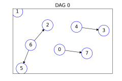
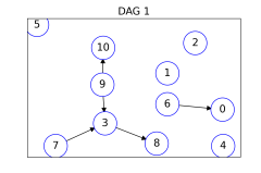
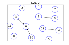
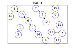
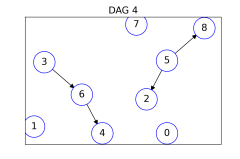
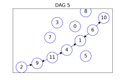
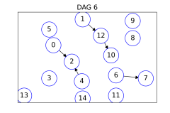
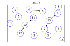
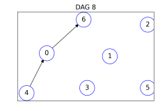
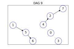
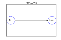
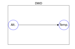
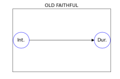
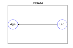
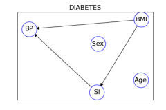
Figure 1: DAGs of synthetic datasets (first and second rows), and DAGs of real-world datasets (third row).

V-A Evaluation Measures

Since the contribution of this paper is twofold, i.e., the definition of an efficient and accurate method for nonlinear causal discovery and the design of a synthetic dataset generator, we need to evaluate and measure the validity of both aspects.

We establish to evaluate the correctness in the causal discovery task following the machine learning fashion [39]. Let $G$ be the real DAG describing the causal structure, and $\tilde{G}$ the DAG inferred with a causal discovery approach. We say that $G_{ij}=1$ if in $G$ exists an edge from the node representing the feature $i$ to the node representing feature $j$, i.e., $i$ causes $j$ ($i\leftarrow j$). Then, if $G_{ij}=\tilde{G}_{ij}=1$ we have a True Positive, if $G_{ij}=\tilde{G}_{ij}=0$ we have a True Negative, if $G_{ij}=0\wedge\tilde{G}_{ij}=1$ a False Positive, and if $G_{ij}=1\wedge\tilde{G}_{ij}=0$ a False Negative. Given these definitions it is easy to define standard evaluation measures such as accuracy, precision, recall, and f1 [36].

On the other hand, we evaluate the correctness of a synthetic dataset generative model using the following measures based on (i) distances or (ii) outlierness [40]. Let $X$ be the real dataset, and $\tilde{X}$ the synthetic one, we use the Sum of Squared Error (SSE) and Root Mean Squared Error (RMSE) as measures based on distances. More in detail, for each feature $j$ we perform the Kernel Density Estimation (KDE) on both $X^{(j)}$ and on $\tilde{X}^{(j)}$ to estimate the Probability Density Function (PDF). We generate a set of 1000 random values according to the PDF, and we compare them using the SSE and the RMSE. Finally, we aggregate the evaluations performed for the various features of the datasets by averaging them. For estimating the number of outliers present in $\tilde{X}$ concerning $X$, we employ the Local Outlier Factor (LOF) [41]. LOF is an outlier detection method that measures the local density deviation of a given instance and compares it to the local densities of its neighbors. Instances that have a density substantially lower than their neighbors are considered to be outliers. In our experiments we check if any instance $\tilde{x}_{i}\in\tilde{X}$ can be considered an outlier concerning the real instances in $X$. If the LOF is lower than one, it means that a higher density surrounds a point than its neighbors, and it is considered an inlier, i.e., an acceptable synthetic record in our setting. On the other hand, the point is considered an outlier.

V-B Synthetic and Real Datasets

In order to carefully perform the aforementioned evaluation, we require ground-truth datasets of various dimensionalities with known causal relationships. This aspect is fundamental in the context of causal discovery. Indeed, to evaluate these methodologies, we need to rely on the structure of the DAG to test the identified causal relationships. However, since the literature lacks this type of information, we developed a generator of random synthetic continuous datasets for which the causal structure is known a priori.

The generator first creates a random DAG $G$ to be used as ground truth. The DAG $G$ is generated by selecting a number of random nodes in $[5,20]$ and a number of random edges in $[2,\mathit{nbr\_nodes}/2]$. Edges are assigned randomly to couples of nodes. Then, it takes as input $G$ and returns a multivariate continuous dataset $X$ respecting the causal relationships where each column in $X$ represents a node in $G$. The synthetic dataset $X$ is generated according to the following steps. First, the features matching isolated and source nodes are generated, i.e., those modeling independent variables. Moreover, the generator adds a uniform noise in $[-1,1]$ to each independent variable. Following the topological ordering of the DAG, we ensure the independent variables are generated before the dependent ones. Second, the features matching dependent variables are generated by combining the parent variables with randomly selected binary functions and by applying to each parent variable a randomly selected nonlinear function among sine, cosine, square root, logarithm, and tangent. Finally, like for independent variables, the generator adds a uniform noise in $[-1,1]$ also to dependent variables.

In our experiments, we generated 10 different DAGs illustrated in Figure 1 ($1^{\mathit{st}},2^{\mathit{nd}}$ rows). For each DAG, we repeated the synthetic data generative procedure ten times, ending up with a total of 100 different synthetic datasets, each one with 1000 instances respecting the causal relationships.

We also experimented with real datasets typically used in papers of causal discovery for which the ground-truth DAG is known. We selected abalone, oldf and dwd from [12], and undata from [10]. In addition, since all these datasets are bivariate, we also considered the multivariate dataset diabets for which we specified the ground-truth DAG. The DAGs for these datasets are in Figure 1 ($3^{\mathit{rd}}$ row).

TABLE I: Runtime and F1-measure for causal discovery on DAGs with increasing number of features. ^∗ not all results considered.

nbr features	Time (sec)			F1-measure
	ncd	ncda	apriori	ncd	ncda
2	$0.454$	$0.462$	$0.004$	$1.000$	$1.000$
3	$5.034$	$0.464$	$0.005$	$1.000$	$1.000$
4	$115.1$	$0.990$	$0.006$	$0.890$	$0.906$
5	$>3600$	$1.033$	$0.007$	$-$	$0.891$
6	$>3600$	$1.229$	$0.008$	$-$	$0.814$
avg	$>3600$	$0.835$	$0.006$	$0.963^{*}$	$0.926$

TABLE II: Runtime and F1-measure for causal discovery on real DAGs.

nbr features	Time (sec)			F1-measure
	ncd	ncda	apriori	ncd	ncda
abalone	$0.208$	$0.207$	$0.008$	$1.000$	$1.000$
oldf	$0.089$	$0.089$	$0.006$	$1.000$	$1.000$
dwd	$0.058$	$0.073$	$0.008$	$1.000$	$1.000$
undata	$0.048$	$0.045$	$0.008$	$1.000$	$1.000$
diabets	$4607$	$10.00$	$0.009$	$0.750$	$0.750$

V-C Baselines

We study the effectiveness of our proposal comparing it against some baselines and state-of-the-art proposals.

In particular, for the task of causal discovery, besides ncd, we compare ncda against coefficients typically used to detect correlations. Indeed, our intuition is that correlation among variables is a clue for causation. Therefore, simple coefficients like Pearson (pc), Spearman (sc) and Hoeffding’s D (hc) [36] could be used in replacement of Apriori. We selected these three correlation indexes because they differ on (i) the type of relationship which are able to recognize, (ii) the direction of the relationship, i.e., monotonic vs. non-monotonic, (iii) the statistic approach, i.e., parametric vs. non-parametric. For the evaluation of the Pearson and Spearman correlations, we checked the p-value using $0.05$ as a threshold, while for Hoeffding’s D, we set the acceptance threshold to $0.03$.

For synthetic data generation, we compared against a random data generator (rnd) that assumes uniform distribution and independence among all the variables. Also, we compare ncda against state-of-the-art data generators of Synthetic Data Vault library. We experimented with tvae [28] and ctgan [29] with default parameters generating 1000 instances.

V-D Experimental Settings

In the experiments we run ncda and gencda with the following parameters: $\mathit{n\_bins}\in[3,10]$, $\mathit{min\_sup}\in[0.05,0.4]$, $\mathit{max\_len}\in\{3,4,5\}$, $\alpha\in\{0.001,0.01,0.02,0.05,0.1\}$. The default parameter justified by the experiments reported in Section V-F is $\mathit{n\_bins}=10$, $\mathit{min\_sup}=0.05$, $\mathit{max\_len}=3$, and $\alpha=0.001$. In gencda as the list of distributions $D$ we consider the following among those available in scipy: uniform, exponweib, expon, gamma, beta, alpha, chi, chi2, laplace, lognorm, norm, powerlaw. A higher number of distributions (each one with its parameters) increases the computation time but also improves the performance as more accurate independent variables can be described. For the ensemble regressor in gencda we rely on the GPR, SVM, kNN, and DTR of scikit-learn trained with default parameters.

TABLE III: Comparison of ncda with correlation coefficients to detect causalities on synthetic DAGs. Best results in bold.

DAG	Accuracy				Precision				Recall
	pc	sc	hc	ncda	pc	sc	hc	ncda	pc	sc	hc	ncda
0	.89	.88	.93	.91	.67	.60	.86	.88	.62	.68	.60	.50
1	.87	.87	.92	.94	.32	.31	.66	.88	.38	.40	.42	.44
2	.92	.91	.95	.97	.23	.21	.63	1.0	.23	.25	.28	.42
3	.88	.87	.92	.97	.10	.10	.14	.92	.17	.19	.12	.53
4	.93	.90	.95	.95	.68	.54	.83	.89	.70	.88	.78	.70
5	.88	.87	.92	.93	.32	.30	.64	.88	.23	.25	.25	.25
6	.90	.90	.90	.97	.16	.15	.38	.93	.20	.28	.29	.52
7	.90	.89	.94	.98	.03	.04	.07	.94	.04	.08	.04	.50
8	.92	.93	.97	.96	.61	.60	.80	.87	.95	1.0	.95	.80
9	.88	.89	.93	.92	.63	.63	.89	.97	.57	.60	.60	.45
avg	.89	.89	.93	.95	.37	.34	.58	.91	.41	.45	.43	.51

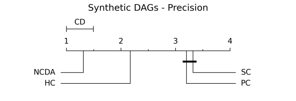
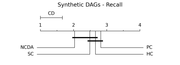
Figure 2: CD plots with Nemenyi at 95% confidence level or synthetic DAGs

TABLE IV: Comparison of ncda with correlation coefficients to detect causalities on real DAGs.

DAG	Accuracy				Precision				Recall
	pc	sc	hc	ncda	pc	sc	hc	ncda	pc	sc	hc	ncda
abalone	$1.0$	$1.0$	$1.0$	$1.0$	$1.0$	$1.0$	$1.0$	$1.0$	$1.0$	$1.0$	$1.0$	$1.0$
oldf	$1.0$	$1.0$	$1.0$	$1.0$	$1.0$	$1.0$	$1.0$	$1.0$	$1.0$	$1.0$	$1.0$	$1.0$
dwd	$1.0$	$1.0$	$1.0$	$1.0$	$1.0$	$1.0$	$1.0$	$1.0$	$1.0$	$1.0$	$1.0$	$1.0$
undata	$1.0$	$1.0$	$1.0$	$1.0$	$1.0$	$1.0$	$1.0$	$1.0$	$1.0$	$1.0$	$1.0$	$1.0$
diabets	$0.4$	$0.4$	$0.8$	$0.9$	$0.3$	$0.3$	$0.6$	$0.6$	$1.0$	$1.0$	$0.6$	$1.0$

V-E Results

The first aspect that we analyze is the impact of apriori on the performance of ncd for the task of causal discovery. In Table I we observe the performance of ncd and ncda in terms of runtime and F1-measure for DAGs with a growing number of features. With ^∗ we indicate that for ncd the average value considers only the cases in which the procedure terminated within an hour. Given a number of features, we randomly generated 50 DAGs and datasets with the approach of Sec. V-B. We notice how ncda has a remarkable improvement in terms of runtime that becomes evident when number of features is higher than 4. Thus, the computational time required by ncda is exponentially lower than the one required by ncd. The third column shows the negligible impact of apriori on the runtime of ncda. Besides, from the F1-measure, we notice that apriori does not impact the performance of ncda to ncd when observing the correctness of the causal relationships discovered in terms of F1-measure. Similar results are on Table II for the real datasets.

In Table III we report the accuracy, precision and recall for the task of causal discovery for the ten synthetic DAGS of Figure 1 ($1^{st}$ and $2^{nd}$ rows) comparing ncda against the correlation indexes Pearson (pc), Spearman (sc) and Hoeffding’s D (hc). We remark that for each DAG, we generate ten different datasets. In Table III we report the average performance among the ten datasets. We immediately notice that ncda has the overall better accuracy. However, accuracy cannot be very informative due to the high number of true negative related to the sparseness of the DAGs. Concerning precision is the best performer on all the DAGs. This aspect is crucial as the causalities identified result to be correct nearly always. Finally, recall ncda is more conservative as it sometimes fails to recognize some causal relationships to correlation indexes. However, the average recall remains higher than the competitors.

TABLE V: Comparison of gencda with generative approaches on synthetic datasets: error measures. Best results in bold.

DAG	SSE				RMSE
	rnd	tvae	ctgan	gencda	rnd	tvae	ctgan	gencda
0	$.629$	.137	$.321$	$.257$	$.018$	$.024$	$.036$	.012
1	$.386$	$.156$	.136	$.138$	$.012$	$.022$	$.021$	.006
2	$.320$	$.176$	$.151$	.082	$.011$	$.025$	$.023$	.006
3	$.496$	.178	$.191$	$.205$	$.016$	$.028$	$.029$	.009
4	$.525$	.091	$.147$	$.172$	$.016$	$.020$	$.025$	.008
5	$.248$	$.095$	$.102$	.074	$.010$	$.019$	$.017$	.005
6	$.431$	.114	$.139$	$.167$	$.013$	$.021$	$.021$	.007
7	$.376$	$.197$	$.122$	.137	$.013$	$.026$	$.021$	.007
8	$.411$	.229	$.206$	$.283$	$.014$	$.029$	$.029$	.009
9	$.435$	$.108$	$.184$	.084	$.015$	$.023$	$.026$	.006
avg	$.426$	.148	$.169$	$.160$	$.014$	$.024$	$.025$	.007

TABLE VI: Comparison of gencda with generative approaches on synthetic datasets: outlier measures. Best results in bold.

DAG	LOF				# Outliers
	rnd	tvae	ctgan	gencda	rnd	tvae	ctgan	gencda
0	$0.660$	$0.459$	$0.673$	0.423	$387$	3	$295$	$44$
1	$324.4$	0.457	$10.59$	$0.463$	$915$	131	$691$	$292$
2	$38.03$	$0.448$	0.322	$0.443$	$982$	107	$424$	$151$
3	$>100$	0.471	$>100$	$0.480$	$888$	125	$569$	$232$
4	$3.078$	$0.462$	$1.323$	0.440	$658$	12	$561$	$156$
5	$>100$	$>100$	$>100$	0.370	$982$	$454$	$704$	405
6	$22.67$	$0.450$	0.377	$0.480$	$845$	14	$428$	$181$
7	$>100$	$>100$	$>100$	$0.480$	$903$	$407$	$533$	123
8	$0.476$	0.464	$0.437$	$0.470$	$244$	2	$270$	$86$
9	$2.667$	$0.463$	$2.008$	0.442	$558$	56	$547$	$116$
med	$7.177^{*}$	$0.460^{*}$	$0.660^{*}$	0.461	$736$	27	$502$	$179$

We analyze Table III with the non-parametric Friedman test that compares the average ranks of the causal discovery methods over multiple datasets w.r.t. the various evaluation measure. The null hypothesis that all methods are equivalent is rejected with $\mathit{p{-}value}{<}0.0001$ for all the measures observed. The comparison of the ranks of all methods against each other is visually represented in Figure 2 with Critical Difference (CD) diagrams [42] Two methods are tied if the null hypothesis that their performance is the same cannot be rejected using the Nemenyi test at $\alpha{=}0.05$. ncda has the best rank for precision with statistically significant performance. On the other hand, ranks are not statistically significant w.r.t. recall, but ncda remains the best performer for these metrics.

In Table IV we report accuracy, precision and recall for the causal discovery task on the five real DAGs of Figure 1 ($3^{rd}$ row) comparing ncda against the correlation indexes Pearson (pc), Spearman (sc) and Hoeffding’s D (hc). Analyzing the results we notice that for the bivariate datasets abalone, oldf, dwd and undata, all the approaches manage to identify the causal direction. However, these good results do not indicate that it is possible to identify causalities by exploiting correlations since this only happens when there is only a single causal dependence. Indeed, for the diabets dataset Pearson and Spearman have bad performance. Hoeffding has good precision and a good recall, but none of them is perfect. Finally, ncda obtains the same perfect results on bivariate datasets and overcomes Hoeffding on diabets as Hoeffding has an F1 of $0.6$ while ncda of $0.75$. The non-parametric Friedman test confirms the statistical significance of the results with a $\mathit{p{-}value}{<}0.0005$ for all the measures observed.

In Tables V, VI and Tables VII, VIII we report the evaluation for the data generation task for synthetic and real datasets, respectively. We highlight that for all these Tables, the non-parametric Friedman test confirms the statistical significance of the results with a $\mathit{p{-}value}{<}0.0001$ for all the measures observed. Besides the measures reported in these Tables and discussed in the following, it is worth mentioning that the runtimes of the generation methods are comparable on the relatively small datasets analyzed, Indeed, the average runtime in seconds for generating synthetic data is $10.3$ for rnd, $19.6$ for tvae, $22.7$ for ctgan, and $16.7$ for gencda. We notice that, as expected, rnd is the fastest approach while tvae and ctgan are the slowest. gencda is the second-fastest performer, which is a valuable property considering the good qualitative results discussed in the following.

In Tables V and VII we observe the performance in terms of error measures (SSE and RMSE, the lower the better) for synthetic and the real datasets obtained by comparing the data distributions as detailed in Section V-A. Table V shows the mean values obtained for the different runs among the ten datasets generated for each DAG. We notice that gencda is the best performer in terms of RMSE for synthetic datasets and the second-best performer in terms of SSE. Indeed, tvae has very good results followed by ctgan and finally by rnd. Therefore, it seems that the neural networks modeling the VAE learned by tvae are somewhat able to capture also the causalities learned by gencda through the ncda procedure. However, concerning tvae, gencda shows a smaller running time and therefore higher usability on a larger dataset. This is due to the fact that gencda learns relationships among variables exploiting patterns and does not need to consider many instances as required by VAEs in tvae. The CD plots on the left in Figure 3 validate these observations: gencda is statistically the best performer for the synthetic datasets while it is comparable with all the others.

In Tables VI and VIII we report the performance in terms of LOF score and of the number of outliers (the lower, the better). We calculated the number of outliers as the number of synthetically generated instances for which LOF is higher than one. Table VI shows the median values for the different runs among the ten datasets generated for each DAG. For LOF, we write $>100$ when the median score is very big. This indicates that more than half of the records synthetically generated are considered outliers by LOF. Thus, the total median values in the last line of Table VI have an asterisk $(*)$ when the aggregation is done without considering these very high values. We immediately notice that gencda is the only method without asterisks indicating that the majority of the population generated has a low LOF: the synthetic records of gencda are fewer outliers than those generated with other methods. Again, these results are underlined by the CD plots on the top right in Figure 3: gencda is the best performer followed by tvae and they are statistically comparable. However, empirically gencda shows better results for synthetic datasets. On the other hand, for real datasets, the performance is comparable among the various methods, but gencda is still ranked first. Concerning the number of outliers, results are comparable but, with the above parameter setting of LOF, tvae generates a slightly lower number of outliers than gencda for synthetic datasets, while the results are comparable for real ones.

TABLE VII: Comparison of gencda with generative approaches on real datasets: error-based measures.

DAG	SSE				RMSE
	rnd	tvae	ctgan	gencda	rnd	tvae	ctgan	gencda
abalone	$.471$	$.080$	$.067$	.035	$.016$	$.025$	$.023$	.005
oldf	$6.05$	.066	$.116$	$5.04$	$.059$	$.020$	$.026$	.056
dwd	$.469$	.075	$.462$	$.185$	$.007$	$.019$	$.015$	.009
undata	$.125$	.019	$.006$	$.051$	$.010$	$.013$	$.006$	.006
diabets	$226$	.000	$.004$	$213$	$1.48$	.001	$.005$	$1.15$

TABLE VIII: Comparison of gencda with generative approaches on real datasets: outlier-based measures.

DAG	LOF				# Outliers
	rnd	tvae	ctgan	gencda	rnd	tvae	ctgan	gencda
abalone	$15.2$	0.11	$0.06$	$9.36$	$145$	$155$	152	$108$
oldf	$0.53$	$0.42$	$0.44$	0.35	$66$	$14$	$59$	13
dwd	$2.27$	0.17	$0.70$	$0.40$	$76$	$24$	$109$	16
undata	$0.31$	$0.45$	0.29	$3.81$	$17$	1	$28$	$192$
diabets	0.25	$0.45$	$0.35$	$0.37$	$42$	1	$16$	$26$

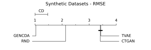
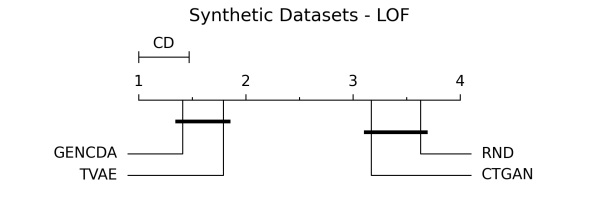
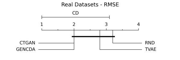
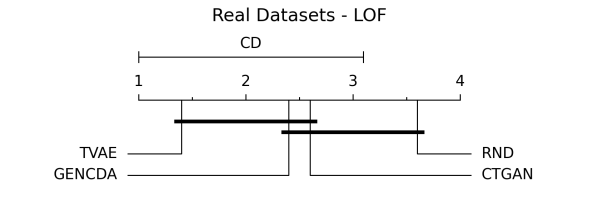
Figure 3: CD plots with Nemenyi at 95% confidence level.

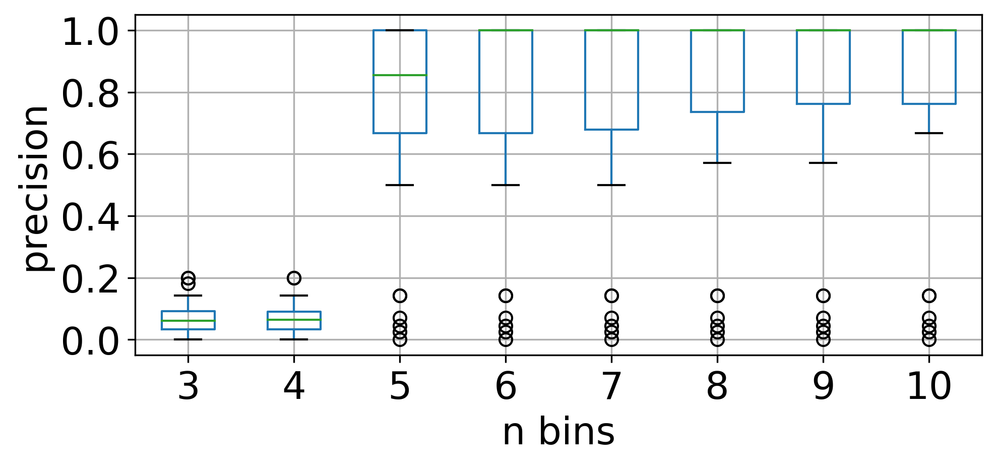
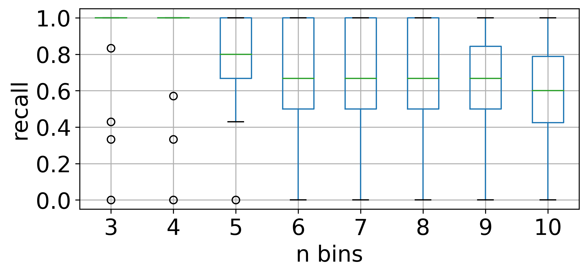
Figure 4: Effect of $\mathit{n\_bins}$ on the performance of ncda.

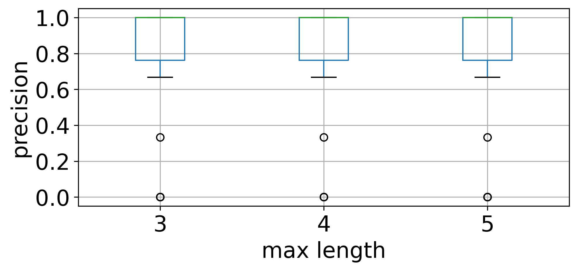
Figure 5: Effect of $\mathit{max\_len}$ on the performance of ncda.

V-F Sensitivity Analysis

We analyze here the parameters mainly affecting the behavior of ncda and gencda. In Figure 4 we observe the boxplots of precision and recall when varying $\mathit{n\_bins}\in[3,10]$ for 50 synthetic DAGs randomly generated. We notice that a higher number of bins improves the precision (and the accuracy), while a lower one only fosters the recall. Since our final objective is to discover causal relationships for data generation, we prefer to be conservative and we consider the causal structure only when we are sure that we have a causal relationship. Therefore, in the experiments we used $\mathit{n\_bins}=10$. In Figure 5 we observe the boxplots of precision when varying $\mathit{max\_len}\in\{3,4,5\}$. We notice that there is no difference in performance (the same applies to accuracy and recall). Hence we use $\mathit{max\_len}=3$ as the default value.

We set $\mathit{min\_sup}=0.05$ for the following reasons. First, from preliminary experimentation emerged that with 50 synthetic DAGs if $\mathit{min\_sup}\geq 0.15$, then the procedure is not able to identify maximal itemsets with at least two items. Second, if $\mathit{min\_sup}=0.1$ it can find maximal itemsets in 44% of the cases, while with $\mathit{min\_sup}=0.05$ this number reaches 92%. With $\mathit{min\_sup}=0.1$ there is a drop in the accuracy with respect to $\mathit{min\_sup}=0.05$ since it excludes itemsets that actually correspond to causal dependencies. Third, considering values of $\mathit{min\_sup}$ lower than $0.05$ highly increases the chances of retrieving patterns not relevant for our task, i.e., taking into account features that are not part of the underlying causal model to the data. Thus, since the verification of a causal relationship is done by ncd we optimize apriori for the task of retrieving the highest possible number of admissible maximal itemsets. Finally, we considered different p-values thresholds $\alpha\in\{0.001,0.01,0.02,0.05,0.1\}$. Since the impact of varying $\alpha$ is negligible, we decided to keep our procedure conservative by setting the lowest value, i.e., $\alpha=0.001$.

VI Conclusion

We have observed how ncda overcomes the limitation of ncd while maintaining comparable performance. Besides, we have shown that gencda produces more realistic synthetic data than those generated with trivial baselines and it is comparable with time-consuming state-of-the-art generators. Also, gencda requires fewer instances than GANs or VAEs and also works on high dimensionality settings. From an applications viewpoint, the exploitation of gencda that provides insights of causal mechanisms will allow circumventing plausibility concerns creating trustful scenarios for developing ML algorithms in critical domains such as healthcare.

Several future research directions are possible. First, we would like to stress gencda with larger datasets and DAGs with more variables. Second, we have focused on continuous datasets, but it would be interesting to extend our proposal to datasets with categorical attributes. Third, gencda is indeed a framework. Thus, it could be interesting to evaluate how it behaves when replacing ncd with other approaches, and/or the ensemble of regressors with another regressor (for instance, a deep neural network) to check if it is possible to improve the performance. Also, it could be interesting to test gencda on other data types. Fourth, it would be nice to investigate if there are theoretical properties related to the filtering through Apriori when searching for causal relationships. Finally, we would like to study the impact of gencda used as a generative procedure of explainability approaches such as lime or lore.

References

- [1] D. Jeske et al., “Synthetic data generation capabilties for testing data mining tools,” in MILCOM, 10 2006, pp. 1–6.
- [2] C. C. Michael et al., “Genetic algorithms for dynamic test data generation,” in ASE. IEEE Computer Society, 1997, pp. 307–308.
- [3] N. V. Chawla et al., “SMOTE: synthetic minority over-sampling technique,” J. Artif. Intell. Res., vol. 16, pp. 321–357, 2002.
- [4] S. J. Pan et al., “A survey on transfer learning,” IEEE Trans. Knowl. Data Eng., vol. 22, no. 10, pp. 1345–1359, 2010.
- [5] M. T. Ribeiro et al., “”why should I trust you?”: Explaining the predictions of any classifier,” in KDD. ACM, 2016, pp. 1135–1144.
- [6] D. S. Yeung et al., “Localized generalization error model and its application to architecture selection for radial basis function neural network,” IEEE Trans. Neural Networks, pp. 1294–1305, 2007.
- [7] W. Ng et al., “Image classification with the use of radial basis function neural networks and the minimization of the localized generalization error,” Pattern Recognition, vol. 40, no. 1, pp. 19–32, 2007.
- [8] R. Guidotti et al., “A survey of methods for explaining black box models,” ACM Comput. Surv., vol. 51, no. 5, pp. 93:1–93:42, 2019.
- [9] I. J. Goodfellow et al., “Generative adversarial nets,” in NIPS, 2014, pp. 2672–2680.
- [10] J. M. Mooij et al., “Distinguishing cause from effect using observational data: Methods and benchmarks,” J. M. L. R., pp. 32:1–32:102, 2016.
- [11] R. Guo et al., “A survey of learning causality with data: Problems and methods,” ACM Comput. Surv., vol. 53, no. 4, pp. 75:1–75:37, 2020.
- [12] P. O. Hoyer et al., “Nonlinear causal discovery with additive noise models,” in NIPS. Curran Associates, Inc., 2008, pp. 689–696.
- [13] J. Pearl, “Causality: Models, reasoning, and inference,” Cambridge University Press, 2000.
- [14] P. Spirtes et al., Causation, Prediction, and Search, Second Edition, ser. Adaptive Computation and M. L. MIT Press, 2000.
- [15] ——, “Causal discovery and inference: concepts and recent methodological advances,” in App. Inf., vol. 3, no. 1, 2016, pp. 1–28.
- [16] S. Shimizu et al., “A linear non-gaussian acyclic model for causal discovery,” J. Mach. Learn. Res., vol. 7, pp. 2003–2030, 2006.
- [17] Z. Chen et al., “Nonlinear causal discovery for high dimensional data: A kernelized trace method,” in ICDM. IEEE C.S., 2013, pp. 1003–1008.
- [18] R. Cai et al., “Causal discovery with cascade nonlinear additive noise models,” CoRR, vol. abs/1905.09442, 2019.
- [19] N. Friedman et al., “Gaussian process networks,” in UAI. Morgan Kaufmann, 2000, pp. 211–219.
- [20] A. Dandekar et al., “A comparative study of synthetic dataset generation techniques,” in DEXA (2), vol. 11030. Springer, 2018, pp. 387–395.
- [21] D. B. Rubin, Multiple imputation for nonresponse in surveys. John Wiley & Sons, 2004, vol. 81.
- [22] T. E. Raghunathan et al., “Multiple imputation for statistical disclosure limitation,” Journal of Official Statistics, vol. 19, no. 1, p. 1, 2003.
- [23] H. He et al., “ADASYN: adaptive synthetic sampling approach for imbalanced learning,” in IJCNN. IEEE, 2008, pp. 1322–1328.
- [24] J. P. Reiter, “Using cart to generate partially synthetic public use microdata,” Journal of Official Statistics, vol. 21, no. 3, p. 441, 2005.
- [25] H. Ping et al., “Datasynthesizer: Privacy-preserving synthetic datasets,” in SSDBM. ACM, 2017, pp. 42:1–42:5.
- [26] N. Patki et al., “The synthetic data vault,” in DSAA. IEEE, 2016, pp. 399–410.
- [27] A. Makhzani et al., “Adversarial autoencoders,” CoRR, vol. abs/1511.05644, 2015.
- [28] L. Xu et al., “Synthesizing tabular data using generative adversarial networks,” CoRR, vol. abs/1811.11264, 2018.
- [29] ——, “Modeling tabular data using conditional GAN,” in NeurIPS, 2019, pp. 7333–7343.
- [30] R. Guidotti et al., “Factual and counterfactual explanations for black box decision making,” IEEE Intell. Syst., vol. 34, no. 6, pp. 14–23, 2019.
- [31] J. Runge et al., “Inferring causation from time series in earth system sciences,” Nature communications, vol. 10, no. 1, pp. 1–13, 2019.
- [32] A. Lawrence et al., “Data generating process to evaluate causal discovery techniques for time series data,” CoRR, vol. abs/2104.08043, 2021.
- [33] Z. Wood-Doughty et al., “Generating synthetic text data to evaluate causal inference methods,” CoRR, vol. abs/2102.05638, 2021.
- [34] A. Gretton et al., “Kernel methods for measuring independence,” J. Mach. Learn. Res., vol. 6, pp. 2075–2129, 2005.
- [35] C. E. Rasmussen et al., Gaussian processes for machine learning, ser. Adaptive computation and machine learning. MIT Press, 2006.
- [36] P. Tan et al., Introduction to Data Mining. Addison-Wesley, 2005.
- [37] R. Agrawal et al., “Fast algorithms for mining association rules in large databases,” in VLDB. Morgan Kaufmann, 1994, pp. 487–499.
- [38] R. W. Robinson, “Counting unlabeled acyclic digraphs,” in Combinatorial Mathematics V. Springer, 1977, pp. 28–43.
- [39] D. Kalainathan et al., “Causal discovery toolbox: Uncovering causal relationships in python,” J. M. L. Res., vol. 21, pp. 37:1–37:5, 2020.
- [40] R. Guidotti et al., “Data-agnostic local neighborhood generation,” in ICDM. IEEE, 2020, pp. 1040–1045.
- [41] M. M. Breunig et al., “LOF: identifying density-based local outliers,” in SIGMOD Conference. ACM, 2000, pp. 93–104.
- [42] J. Demsar, “Statistical comparisons of classifiers over multiple data sets,” J. Mach. Learn. Res., vol. 7, pp. 1–30, 2006.