Hierarchical Bayesian inference for community detection and connectivity of functional brain networks

Abstract

Many functional magnetic resonance imaging (fMRI) studies rely on estimates of hierarchically organised brain networks whose segregation and integration reflect the dynamic transitions of latent cognitive states. However, most existing methods for estimating the community structure of networks from both individual and group-level analysis neglect the variability between subjects and lack validation. In this paper, we develop a new multilayer community detection method based on Bayesian latent block modelling. The method can robustly detect the group-level community structure of weighted functional networks that give rise to hidden brain states with an unknown number of communities and retain the variability of individual networks. For validation, we propose a new community structure-based multivariate Gaussian generative model convolved with haemodynamic response function to simulate synthetic fMRI signal. Our result shows that the inferred community memberships using hierarchical Bayesian analysis are consistent with the predefined node labels in the generative model. The method is also tested using real working memory task-fMRI data of 100 unrelated healthy subjects from the Human Connectome Project. The results show distinctive community structures and subtle connectivity patterns between 2-back, 0-back, and fixation conditions, which may reflect cognitive and behavioural states under working memory task conditions.

Keywords: fMRI, brain networks, community detection, latent block model, Bayesian inference, Markov chain Monte Carlo

1 Introduction

Brain function or cognition can be described in terms of multiscale hierarchical organization (Kringelbach and Deco, , 2020), from neurons and macrocolumns to macroscopic brain areas (Park and Friston, , 2013). The functional connectivity (FC) is a measure of statistical dependence between regional time series, typically based on the blood oxygen level-dependant (BOLD) signal, and may show prominently discrepant patterns between different subjects (Monti et al., , 2017, Betzel et al., , 2019, Bian et al., , 2021). These discrepant patterns of FC are not only caused by changes in latent cognitive states including mental processes (Taghia et al., , 2018, Hutchison et al., , 2013) (e.g., thoughts, ideas, awareness, arousal, and vigilance) occurring at an unpredictable timescale during the resting state (Hutchison et al., , 2013, Allen et al., , 2014, Calhoun et al., , 2014, Friston et al., , 2014, Razi et al., , 2015, Razi and Friston, , 2016, Razi et al., , 2017, Power et al., , 2017, Parkes et al., , 2018, Aquino et al., , 2020, Friston et al., , 2021, Lurie et al., , 2020) and brain activity responding to an external stimulus during task (Cribben et al., , 2012, Gonzalez-Castillo and Bandettini, , 2018, Vidaurre et al., , 2018), but also due to non-neural physiological factors such as head motion, cardiovascular, and respiratory effects or the noise coming from the hardware instability (Hutchison et al., , 2013, Lurie et al., , 2020). Both the changes in cognitive states and noise affect the transient functional interaction between pairs of nodes, which will further result in significant changes in the community structure of brain networks (Bassett et al., , 2013, Cribben and Yu, , 2017, Robinson et al., , 2015, Betzel et al., , 2018, Ting et al., , 2021, Bian et al., , 2021). One outstanding problem is the unreliability of single-subject estimate of functional interactions between brain regions because it ignores information that is shared across individuals (Lehmann et al., , 2021). Even in task fMRI, although the performance of participants is constrained by an external stimulus, the latent intrinsic mental processes and the noise inevitably affect the metrics of individual functional interactions. Therefore, it is important to consider the group-level community structure to depict the hierarchical brain networks and quantify the between-subject variability of functional connectivity during a task. This can help alleviate the random influence of intrinsic mental processes and external non-neural noise.

In fMRI studies, several community-detection methods have been employed to characterize brain states in functional networks. For example, a stochastic block model combined with non-overlapping sliding windows was applied to infer dynamic FC for networks, where edge weights were estimated by averaging the coherence matrices over subjects and a threshold was applied to binarize the FC (Robinson et al., , 2015). However, this approach may not retain complete information of the time series and lack the evaluation of inter-subject variability. To robustly detect the community structure of functional brain networks, recent studies have begun to focus on multiple networks from different subjects and estimate common features of network patterns using group-level analysis to reduce uncertainty caused by intrinsic cognitive state and non-neural noise. One of the popular community detection methods for group-level analysis is based on multilayer modularity (Bassett et al., , 2011, 2013). Another method based on a multi-subject stochastic block modelling can flexibly evaluate inter-individual variations in the community structure of functional networks (Pavlović et al., , 2020), but also treats the functional connectivity as binary edges. Other techniques that can capture the dynamics of brain networks at both the individual and group level by taking into account between-subject variations in BOLD time series include Ting et al., (2021) and Betzel et al., (2019).

Modelling complex system dynamics plays an essential role in characterizing the brain mechanisms and processes that are not directly observable. For example, mean-field models (Deco et al., , 2008) can be regarded as a forward model which can be inverted given the empirical data. Setting the model parameters appropriately makes assumptions about the latent large-scale networks and may facilitate the description about the generation of spatiotemporal activity observed in BOLD signal (Jirsa et al., , 2010). Other extensive realistic simulations of fMRI data using generative modelling for a variety of proposed networks, experimental designs and confounds underlying the empirical data were proposed in Smith et al., (2011).

In our previous work (Bian et al., , 2021), a Bayesian change-point detection method was developed to identify the transitions of brain states. For each inferred brain state, the group-averaged adjacency matrix was calculated as an observation which preserved complete information about the time series of the subjects. However, we neglected the variability of FC between different subjects and ignored the higher-order topological properties of individual’s network. A Bayesian (Gaussian) latent block model (LBM) was used to detect the community structure of each discrete brain state, where the community memberships were inferred by Markov chain Monte Carlo (MCMC) sampling (Metropolis et al., , 1953, Hastings, , 1970) with a predetermined number of communities estimated by model selection.

In this paper, we present a new method based on hierarchical Bayesian modelling to capture the variability between subjects at the group level. We use the LBM to characterize individual-level FC and infer a latent label vector by MCMC sampling with an unknown number of communities with absorption and ejection strategy (Nobile and Fearnside, , 2007, Wyse and Friel, , 2012) to estimate the multilayer community structure that underlies a specific brain state for the group. Here, a layer of community structure corresponds to an individual’s functional brain network. At the group level, we model the estimated latent label vectors by a Categorical-Dirichlet conjugate pair and define a maximum label assignment probability matrix (MLAPM) providing information about the group-level community structure. We finally model individual-level FC using a Normal-Normal-Inverse-Gamma (Normal-NIG) conjugate pair and estimate the mean and variance connectivity to characterize the group-level functional brain networks or the group representative networks.

For validating its performance, we simulate fMRI data using a multivariate Gaussian generative model convolved with a haemodynamic response function (Smith et al., , 2011, Bian et al., , 2021), where a covariance matrix encodes the ground truth of community memberships and inter- and intra-community densities. We find that the MLAPM estimates are consistent with the ground truth of both the latent label vectors and the number of communities predefined in the generative model used to simulate the synthetic fMRI data.

We further apply our method to working memory task-fMRI data from the Human Connectome Project (Van Essen et al., , 2013, Barch et al., , 2013) to estimate the community structure of discrete brain states and the (weighted) connectivity at the group level. The estimated community structures of discrete brain states show distinctive patterns between 2-back, 0-back, and fixation conditions in a working-memory task-based fMRI experiment.

This paper presents three main contributions: (i) We proposed a novel hierarchical Bayesian modelling method based on latent block modelling and MCMC sampling with absorption and ejection strategy. Our method can estimate the community structure of group representative network with an unknown number of communities while accounting for the inter-subject variability. (ii) We modelled the group-level brain connectivity based on Bayesian conjugate analysis that can capture both the mean strength and variation of group representative network. (iii) We proposed a novel generative model to simulate synthetic fMRI data with assumptive latent community structure and inter- and intra-community connectivity densities modelling the spatiotemporal segregation and integration of sub-networks of brain states.

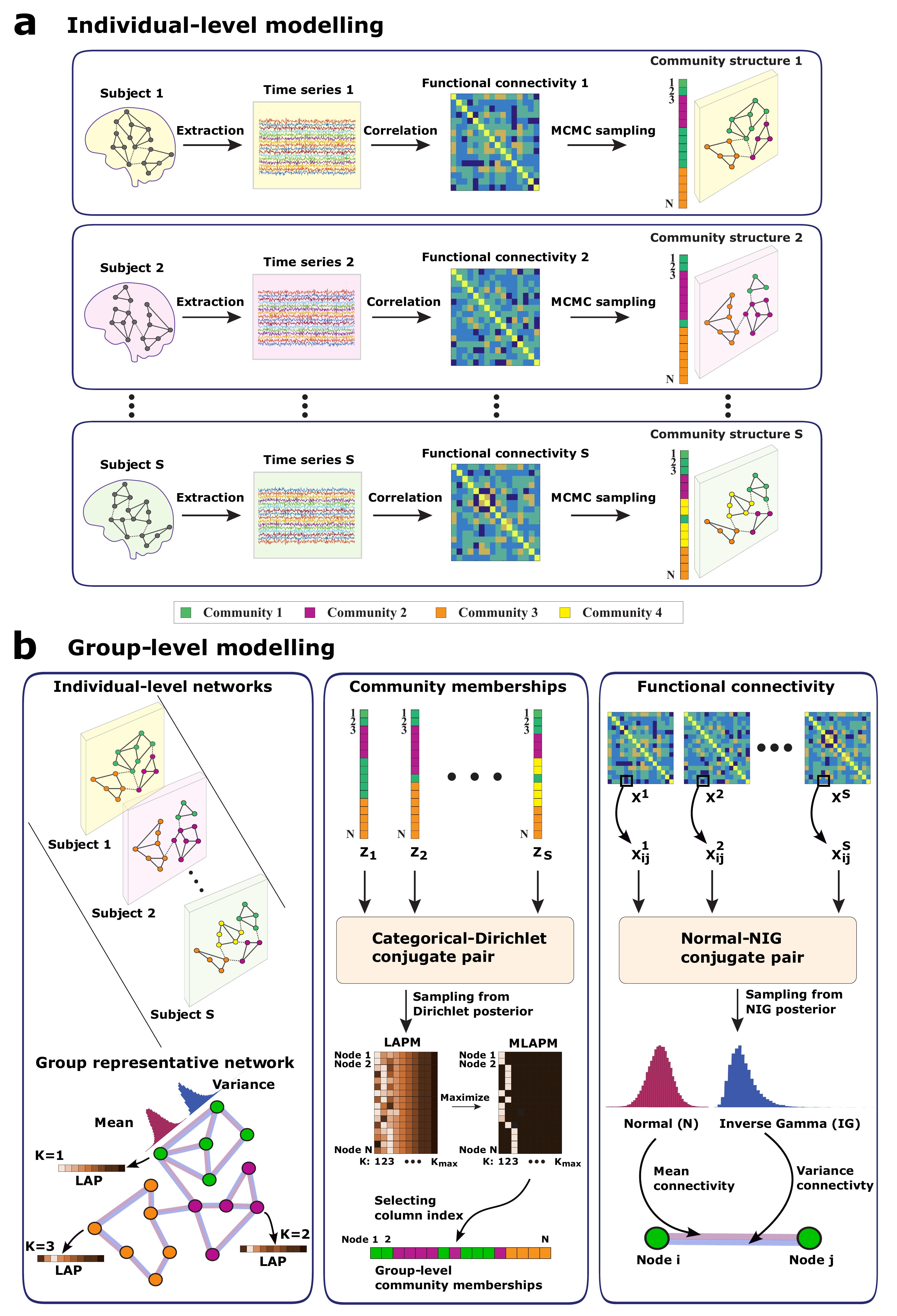
Fig. 1: Multilayer community detection for functional brain networks. a Individual-level modelling. For real data analysis, the BOLD time series are extracted from brain regions of interest for each subject. For synthetic data analysis, the time series are simulated from generative models with known community structures. The functional connectivity (a weighted adjacency matrix) is computed via Pearson’s correlation from the regional time series. The community memberships of the network are estimated by drawing latent label vectors from a posterior density using MCMC sampling for each subject. Nodes belonging to the same community are shown in same colour. b Group-level modelling. We analyze the group representative network from all of the subjects (from subject 1 to $S$). The community memberships $\{\bm{z}_{1},\cdots,\bm{z}_{s}\}$ estimated for each individual are treated as realizations of a latent group-level community structure. A Bayesian model with categorical-Dirichlet pair is used to fit the community memberships and a maximum label assignment probability matrix (MLAPM) is calculated by maximizing a label assignment probability matrix (LAPM), which contains the information about the community structure at the group level. Each row in LAPM is a vector of label assignment probabilities (LAP) for a specific node. Finally, we model the FC of discrete brain states. A Normal-NIG conjugate pair is used to model the connectivity $\bm{X}_{ij}=\{x_{ij}^{1},x_{ij}^{2},\cdots,x_{ij}^{S}\}$ from $S$ subjects for a specific pair of nodes. The mean and variance connectivity at the group level are estimated by drawing samples from the Normal (N) and Inverse Gamma (IG) posterior densities respectively.

2 Methods

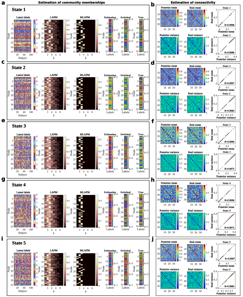
Fig. 1: Validation of group-level community memberships and connectivity estimates using synthetic fMRI data (5dB). This figure is in the same format as Fig.2 in the main text only that it is the experimental result with 5dB.

We develop a novel multilayer community detection method (Fig.1) based on hierarchical Bayesian modelling to robustly estimate the community memberships and the number of communities of functional brain networks at the group level while accounting for inter-individual variation. In Bayesian inference, the posterior distribution is obtained by combining prior and likelihood. If the prior and posterior follow from the same distribution family, then we can say the prior is a conjugate for the likelihood or call them a prior-likelihood conjugate pair. We will first illustrate how to model the adjacency matrix of each subject with a latent block model and how to estimate the individual-level community memberships using the MCMC strategy (Fig.1a). Then we will illustrate the details of using conjugate Bayesian pairs to model the estimated individual-level community memberships and individual adjacency matrices respectively. Finally, we perform parameter inference by drawing samples from posterior densities to depict the group representative network including the group-level community structure and a group-level FC (Fig.1b).

2.1 Individual-level modelling of the community structure

We first use a latent block model (LBM) (Wyse and Friel, , 2012, Bian et al., , 2020, 2021) to model a weighted adjacency matrix $\bm{x}\in\mathbb{R}^{N\times N}$ measuring the FC of a specific brain state for each subject, where $N$ denotes the number of nodes which are assigned to $K$ communities. Suppose that $K$ is a random variable following a Poisson distribution. We denote the community memberships as a latent label vector $\bm{z}=(z_{1},\ldots,z_{i},\ldots,z_{N})$ where $z_{i}\in\{1,\cdots,K\}$ is the label of node $i$. Each $z_{i}$ independently follows a categorical (one-trial multinomial) distribution:

$$z_{i}\sim\mbox{Categorical}(1;\bm{r}=(r_{1},\cdots,r_{k},\cdots,r_{K})),$$ (2.1)

where $\bm{r}$ is a vector, the element $r_{k}$ is the probability of a node being assigned to community $k$, and $\sum_{k=1}^{K}r_{k}=1$. The categorical probability can be written using the indicator function $I_{k}(z_{i})$ as

$$p(z_{i}|\bm{r},K)=\prod_{k=1}^{K}r_{k}^{I_{k}(z_{i})},\mbox{where\ }I_{k}(z_{i})=\begin{cases}1,\ \mbox{if}\ z_{i}=k\\ 0,\ \mbox{if}\ z_{i}\neq k\\ \end{cases}.$$ (2.2)

The density of the $N$-dimensional latent label vector $\bm{z}$ is

$$p(\bm{z}|\bm{r},K)=\prod_{k=1}^{K}r_{k}^{m_{k}(\bm{z})},$$ (2.3)

where $m_{k}(\bm{z})=\sum_{i=1}^{N}I_{k}(z_{i})$. The assignment probability vector $\bm{r}=(r_{1},\cdots,r_{k},\cdots,r_{K})$ follows a $K$-dimensional Dirichlet distribution

$$p(\bm{r}|K)=N(\bm{\alpha})\prod_{k=1}^{K}r_{k}^{\alpha_{k}-1},$$ (2.4)

where $N(\bm{\alpha})=\frac{\Gamma(\sum_{k=1}^{K}\alpha_{k})}{\prod_{k=1}^{K}\Gamma(\alpha_{k})}$ is the normalization factor. We assume that the community assignment is equally likely a priori before observing the data, and we set $\alpha_{k}=1$ for $k=1,\ldots,K$ throughout the paper such that $\bm{r}$ follows the flat Dirichlet distribution with $p(\bm{r}|K)=(K-1)!$.

We define the submatrix $\bm{x}_{kl}$ containing the weighted edges connecting the nodes in community $k$ to the nodes in community $l$, where $k,l\in\{1,\cdots,K\}$. The likelihood of the LBM can be written as

$$p(\bm{x}|\bm{\pi},\bm{z},K)=\prod_{k.l}p(\bm{x}_{kl}|\pi_{kl},\bm{z},K),$$ (2.5)

and the likelihood in specific blocks

$$p(\bm{x}_{kl}|\pi_{kl},\bm{z},K)=\prod_{\{i|z_{i}=k\}}\prod_{\{j|z_{j}=l\}}p(x_{ij}|\pi_{kl},\bm{z},K),$$ (2.6)

where $\bm{\pi}=\{\pi_{kl}\}$ is a $K\times K$ model parameter matrix that is further characterized in the following section.

2.1.1 The latent block model with weighted edges

For weighted edges, the block model parameter in block $kl$ consists of the block mean and variance $\pi_{kl}=(\mu_{kl},\sigma_{kl}^{2})$. Each $x_{ij}$ in the block $kl$ follows a Gaussian distribution conditional on the community number $K$ and the latent label vector $\bm{z}$, that is

$$x_{ij}|\pi_{kl},\bm{z},K\sim\mathcal{N}(\mu_{kl},\sigma_{kl}^{2}).$$

The model parameter $\pi_{kl}=(\mu_{kl},\sigma_{kl}^{2})$ is assumed to independently follow the conjugate Normal-Inverse-Gamma (NIG) prior $\pi_{kl}\sim\mbox{NIG}(\xi,\kappa^{2}\sigma_{kl}^{2},\nu/2,\rho/2)$. That is $\mu_{kl}\sim\mathcal{N}(\xi,\kappa^{2}\sigma_{kl}^{2})$ and $\sigma_{kl}^{2}\sim\mbox{IG}(\nu/2,\rho/2)$. We define $s_{kl}(\bm{x})$ to be the sum of the edge weights in the block $kl$

$$s_{kl}(\bm{x})=\sum_{i:z_{i}=k}\sum_{j:z_{j}=l}x_{ij},$$ (2.7)

and $q_{kl}(\bm{x})$ to be the sum of squares

$$q_{kl}(\bm{x})=\sum_{i:z_{i}=k}\sum_{j:z_{j}=l}x_{ij}^{2}.$$ (2.8)

We also define $w_{kl}(\bm{z})=m_{k}(\bm{z})m_{l}(\bm{z})$ to be the number of elements in the block, where $m_{k}$ and $m_{l}$ are the numbers of nodes in community $k$ and $l$ respectively.

2.1.2 The collapsed posterior of the latent block model

Our aim is to infer latent label vector $\bm{z}$ and the number of communities $K$ by drawing samples from the collapsed posterior $p(\bm{z},K|\bm{x})$ (MacDaid et al., , 2012, Wyse and Friel, , 2012) which can be constructed by integrating out nuisance parameters. The number of communities $K$ follow a Poisson distribution $p(K)=\frac{\lambda^{K}}{K!}e^{-\lambda}$ where $K>0$ and we set $\lambda=1$. We start the derivation of the collapsing procedure with a joint density

$$p(\bm{x},\bm{\pi},\bm{z},\bm{r},K)=p(K)p(\bm{z},\bm{r}|K)p(\bm{x},\bm{\pi}|\bm{z}).$$ (2.9)

The parameters $\bm{r}$ and $\bm{\pi}$ can be collapsed to obtain the marginal density $p(\bm{x},\bm{z},K)$ and the collapsed posterior $p(\bm{z},K|\bm{x})$ is proportional to $p(\bm{x},\bm{z},K)$ as follows

$$p(\bm{z},K|\bm{x})\propto p(\bm{z},K,\bm{x})=p(K)\int p(\bm{z},\bm{r}|K)d\bm{r}\prod_{k,l}\int p(\bm{x}_{kl},\pi_{kl}|\bm{z})d\pi_{kl}.$$ (2.10)

The first integral $p(\bm{z}|K)=\int p(\bm{z},\bm{r}|K)d\bm{r}$ is over the $K$-simplex $\{\bm{r}\!:\!\sum_{k=1}^{K}r_{k}=1\}$ and can be calculated as

$$\int p(\bm{z},\bm{r}|K)d\bm{r} = \frac{\Gamma(\sum_{k=1}^{K}\alpha_{k})}{\Gamma(\sum_{k=1}^{K}(\alpha_{k}+m_{k}(\bm{z}))}\prod_{k=1}^{K}\frac{\Gamma(\alpha_{k}+m_{k}(\bm{z}))}{\Gamma(\alpha_{k})},$$ (2.11)

while the second integral over $\pi_{kl}$ is

$$\int p(\bm{x}_{kl},\pi_{kl}|\bm{z})d\pi_{kl} = \frac{\rho^{\nu/2}\Gamma\{(w_{kl}+\nu)/2\}}{\pi^{w_{kl}/2}\Gamma(\nu/2)(w_{kl}\kappa^{2}+1)^{1/2}}$$ (2.13)

$$\times(-\frac{\kappa^{2}(s_{kl}+\xi/\kappa^{2})^{2}}{w_{kl}\kappa^{2}+1}+\frac{\xi^{2}}{\kappa^{2}}+q_{kl}+\rho)^{-(w_{kl}+\nu)/2}.$$

See the detailed derivation of the above two integrals in Bian et al., (2021).

2.1.3 Estimation of community structure at the individual level

The estimation of the community structure at the individual level involves sampling a latent label vector $\bm{z}$ from the collapsed posterior distribution given the individual adjacency matrix $\bm{x}$ for each subject. There are several proposals for updating the latent label vector using the MCMC method, which constructs a chain of $\bm{z}$ samples converging to the collapsed posterior $p(\bm{z}|\bm{x},K)$. The strategies for updating $\bm{z}$ depend on whether $K$ is treated as a constant or a random variable. For invariant $K$, the number of communities is constant and possible updates include the Gibbs move and the M3 move. For variant $K$, the moves are the absorption move and ejection move (Nobile and Fearnside, , 2007). For individual-level inference, we integrate these four kinds of moves into the Metropolis-Hastings algorithm (Hastings, , 1970).

MCMC allocation sampler with invariant $K$

We first elaborate on the update of the latent label vector $\bm{z}$ with proposal $p(\bm{z}\rightarrow\bm{z}^{\ast})$ (Nobile and Fearnside, , 2007) where $K$ is a fixed number. In the Metropolis-Hastings algorithm (Hastings, , 1970), a candidate latent label vector $\bm{z}^{\ast}$ is accepted with probability $\min\{1,r\}$, where

$$r=\frac{p(K,\bm{z}^{\ast},\bm{x})p(\bm{z}^{\ast}\rightarrow\bm{z})}{p(K,\bm{z},\bm{x})p(\bm{z}\rightarrow\bm{z}^{\ast})}.$$ (2.14)

Gibbs move: At each Gibbs move, one entry $z_{i}$ is randomly selected from $\bm{z}$ and updated by drawing from

$$p(z_{i}^{\ast}|\bm{z}_{-i},\bm{x},K)=\frac{1}{C}p(z_{1},\cdots,z_{i-1},z_{i}^{\ast}=k,z_{i+1},\cdots,z_{N}|\bm{x}),$$ (2.15)

where $k\in\{1,\cdots,K\}$, and $\bm{z}_{-i}$ represents the elements in $\bm{z}$ apart from $z_{i}$. The normalization term can be written as

$$C=p(\bm{z}_{-i}|\bm{x},K)=\sum_{k=1}^{K}p(z_{1},\cdots,z_{i-1},z_{i}^{\ast}=k,z_{i+1},\cdots,z_{N}|\bm{x}).$$ (2.16)

For the Metropolis-Hastings sampler with Gibbs move, the acceptance ratio is $r=1$.

M3 move: The M3 move can update multiple entries of the latent label vector $\bm{z}$. Two communities $k_{1}$ and $k_{2}$ are randomly selected in $\bm{z}$. We define a list $I=\{i,z_{i}=k_{1}\mbox{\ or\ }z_{i}=k_{2}\}$ with length $L$, and a vector of the labels apart from the list $\widetilde{\bm{z}}$. For the update, one element $z_{i}$ is randomly selected from the list and updated according to a reassignment probability $P_{k}^{i}$ as follows

$$\frac{P_{k_{1}}^{i}}{P_{k_{2}}^{i}} = \frac{P_{k_{1}}^{i}}{1-P_{k_{1}}^{i}}$$ (2.17)

$$= \frac{p(z_{i}^{\ast}=k_{1},\widetilde{\bm{z}}|K)}{p(z_{i}^{\ast}=k_{2},\widetilde{\bm{z}}|K)}\frac{p(\widetilde{\bm{x}},\bm{x}^{\ast i}|z_{i}^{\ast}=k_{1},\widetilde{\bm{z}},K)}{p(\widetilde{\bm{x}},\bm{x}^{\ast i}|z_{i}^{\ast}=k_{2},\widetilde{\bm{z}},K)}.$$ (2.18)

Then, $z_{i}^{\ast}$ will be collected into $\widetilde{\bm{z}}$ at the next iteration. The observation $\widetilde{\bm{x}}$ corresponds to $\widetilde{\bm{z}}$ and the observation $\bm{x}^{{\ast}i}$ corresponds to the updated $z_{i}^{\ast}$. The ratio of the proposal can be written as

$$\frac{p(\bm{z}^{\ast}\rightarrow\bm{z})}{p(\bm{z}\rightarrow\bm{z}^{\ast})} = \prod_{i\in I}\frac{P_{z_{i}}^{i}}{P_{z_{i}^{\ast}}^{i}}.$$ (2.19)

For the detailed derivation of the M3 move, one can refer to the previous work in Bian et al., (2021).

MCMC allocation sampler with variant $K$

We can sample $K$ along with the latent label vector $\bm{z}$ from the collapsed posterior $p(\bm{z},K|\bm{x})$ with proposal $p(\{\bm{z},K\}\rightarrow\{\bm{z}^{\ast},K^{\ast}\})$ consisting of the absorption/ejection move (Nobile and Fearnside, , 2007) that changes $K$. A candidate is accepted with probability $\min\{1,r\}$, where

$$r=\frac{p(K^{\ast},\bm{z}^{\ast},\bm{x})p(\{\bm{z}^{\ast},K^{\ast}\}\rightarrow\{\bm{z},K\})}{p(K,\bm{z},\bm{x})p(\{\bm{z},K\}\rightarrow\{\bm{z}^{\ast},K^{\ast}\})}.$$ (2.20)

In the ejection move, a community ejects another community, and in the absorption move, a community absorbs another community. If $\{\bm{z},K\}\rightarrow\{\bm{z}^{\ast},K^{\ast}\}$ is the ejection move with acceptance probability $\min\{1,r\}$, then the inverse move $\{\bm{z}^{\ast},K^{\ast}\}\rightarrow\{\bm{z},K\}$ is the absorption move with acceptance probability $\min\{1,\frac{1}{r}\}$. Suppose that the maximum possible number of communities in the Markov chain is $K_{max}$ and we have $P_{K}^{E}$ chance to choose ejection move and $1-P_{K}^{E}$ chance to choose absorption move. If $K=K_{max}$ for the vector $\bm{z}$ at the current state, there must be an absorption move ($P_{K_{max}}^{E}=0$). For the current state of the latent label vector with $K=1$, there must be an ejection move ($P_{1}^{E}=1$). For $K=2,\cdots,K_{max}-1$, we set the probability of the ejection move as $P_{K}^{E}=0.5$.

Ejection move: We propose the ejection move $\{\bm{z},K\}\rightarrow\{\bm{z}^{\ast},K^{\ast}\}$, where $K^{\ast}=K+1$. For current state $\{\bm{z},K\}$, the ejecting community $k_{1}$ is randomly selected from $K$ communities. The ejected community is labelled with $k_{2}=K+1$. The labels in the ejecting community are reassigned to $k_{1}$ with probability $p_{e}\sim\mbox{Beta}(a,a)$ or $k_{2}$ with probability $1-p_{e}$, we set $a=1$ in this paper. The proposal for the ejection move can be written as

$$p(\{\bm{z},K\}\rightarrow\{\bm{z}^{\ast},K^{\ast}\})=P_{K}^{E}\frac{1}{K}\frac{\Gamma(2a)}{\Gamma(a)\Gamma(a)}\frac{\Gamma(a+\widetilde{m}_{k_{1}})\Gamma(a+\widetilde{m}_{k_{2}})}{\Gamma(2a+\widetilde{m}_{k_{1}}+\widetilde{m}_{k_{2}})},$$ (2.21)

where $\widetilde{m}_{k_{1}}$ and $\widetilde{m}_{k_{2}}$ are the number of elements reassigned to community $k_{1}$ and $k_{2}$ respectively.

Absorption move: For the absorption move $\{\bm{z}^{\ast},K^{\ast}\}\rightarrow\{\bm{z},K\}$ where $K=K^{\ast}-1$, the absorbing community $k_{1}$ is randomly selected from the rest of $K$ communities and the absorbed community is $k_{2}=K^{\ast}$. All the elements in $k_{2}$ are reassigned to $k_{1}$. The proposal for the absorption move can be expressed as

$$p(\{\bm{z}^{\ast},K^{\ast}\}\rightarrow\{\bm{z},K\})=(1-P_{K}^{E})\frac{1}{K}.$$ (2.22)

In MCMC sampling for individual-level inference, we randomly select these four kinds of moves with equal probability to update the latent label vector $\bm{z}$. The latent label vectors are sampled from the Markov chain after a predefined burn-in iteration to ensure the convergence of the chain, and with a specific auto-correlation time between the samples. The inferred $\bm{z}$ will be the estimation of individual-level community memberships. In the next section, we will illustrate the group-level modelling and how to characterize the group-level community structure.

2.2 Group-level modelling of the community structure and connectivity

In this section, we model the community memberships which are estimated from the individual-level analysis. We consider the functional brain networks of all subjects and take individual community memberships (latent label vectors) as our observation for the group-level analysis (see in Fig.1b).

2.2.1 Modelling community memberships

For group-level analysis, we define a matrix

$$\bm{Z}=\begin{pmatrix}z_{11}&\cdots&z_{1s}&\cdots&z_{1S}\\ \vdots&\ddots&\vdots&\ddots&\vdots\\ z_{i1}&\cdots&z_{is}&\cdots&z_{iS}\\ \vdots&\ddots&\vdots&\ddots&\vdots\\ z_{N1}&\cdots&z_{Ns}&\cdots&z_{NS}\\ \end{pmatrix}$$ (2.23)

to represent the latent labels for all of the subjects estimated from the individual-level analysis, where $N$ is the number of nodes and $S$ is the number of subjects. The row vector $\bm{z}_{i}$ contains the labels of the group for a specific node $i$, and the column vector $\bm{z}_{s}$ represents the labels of a specific subject $s$ in the group. In group-level modelling, we model $\bm{z}_{i}=(z_{i1},\cdots,z_{is},\cdots,z_{iS})$ for $S$ subjects for node $i$ using a categorical-Dirichlet conjugate pair. Each label $z_{is}$ follows a categorical distribution $z_{is}\sim\mbox{Categorical}(1;\bm{r}_{i})$ where $\bm{r}_{i}=(r_{i1},\cdots,r_{ik},\cdots,r_{iK})$ is a vector of label assignment probabilities (LAP) such that $\sum_{k=1}^{K}r_{ik}=1$, and $K$ is the maximum element in $\bm{Z}$ in the group. We define a label assignment probability matrix (LAPM)

$$\bm{R}=\begin{pmatrix}r_{11}&\cdots&r_{1k}&\cdots&r_{1K}\\ \vdots&\ddots&\vdots&\ddots&\vdots\\ r_{i1}&\cdots&r_{ik}&\cdots&r_{iK}\\ \vdots&\ddots&\vdots&\ddots&\vdots\\ r_{N1}&\cdots&r_{Nk}&\cdots&r_{NK}\\ \end{pmatrix},$$ (2.24)

and

$$p(z_{is}|\bm{r}_{i},K)=\prod_{k=1}^{K}r_{k}^{I_{k}(z_{is})},\mbox{where\ }I_{k}(z_{is})=\begin{cases}1,\ \mbox{if}\ z_{is}=k\\ 0,\ \mbox{if}\ z_{is}\neq k\\ \end{cases}.$$ (2.25)

Consider a prior Dirichlet distribution $\bm{r}_{i}\sim\mbox{Dirichlet}(\bm{\alpha})$

$$p(\bm{r}_{i}|K)=N(\bm{\alpha})\prod_{k=1}^{K}r_{k}^{\alpha_{k}-1},$$ (2.26)

with the normalization factor $N(\bm{\alpha})=\frac{\Gamma(\sum_{k=1}^{K}\alpha_{k})}{\prod_{k=1}^{K}\Gamma(\alpha_{k})}$. We set $\alpha_{k}=1$. Then the posterior can be formulated as

$$p(\bm{r}_{i}|\bm{z}_{i},K) \propto \prod_{s=1}^{S}p({z}_{is}|\bm{r}_{i})p(\bm{r}_{i})$$ (2.27)

$$= \prod_{s=1}^{S}\prod_{k=1}^{K}r_{k}^{I_{k}(z_{is})}N(\bm{\alpha})\prod_{k=1}^{K}r_{k}^{\alpha_{k}-1}$$ (2.28)

$$= N(\bm{\alpha})\prod_{k=1}^{K}r_{k}^{\sum_{s=1}^{S}I_{k}(z_{is})+\alpha_{k}-1}$$ (2.29)

$$= \frac{N(\bm{\alpha})}{N(\bm{\alpha}^{\prime})}N(\bm{\alpha}^{\prime})\prod_{k=1}^{K}r_{k}^{\sum_{s=1}^{S}I_{k}(z_{is})+\alpha_{k}-1},$$ (2.30)

where $\bm{\alpha}^{\prime}=\sum_{s=1}^{S}I_{k}(z_{is})+\alpha_{k}$, and $N(\bm{\alpha}^{\prime})=\frac{\Gamma(\sum_{k=1}^{K}(\sum_{s=1}^{S}I_{k}(z_{is})+\alpha_{k}))}{\prod_{k=1}^{K}\Gamma(\sum_{s=1}^{S}I_{k}(z_{is})+\alpha_{k})}$. Therefore, we have the posterior $\bm{r}_{i}|\bm{z}_{i}\sim\mbox{Dirichlet}(\bm{\alpha}^{\prime})$. The posterior for the network can be expressed as

$$p(\bm{R}|\bm{Z},K)=\prod_{i=1}^{N}p(\bm{r}_{i}|\bm{z}_{i},K).$$ (2.31)

We use the maximum LAPM (MLAPM) $\bm{R}_{\mbox{max}}$, the maximum probability at each row of the matrix in $\bm{R}$, to provide the information of community structure.

2.2.2 Modelling connectivity

We denote $\bm{X}_{ij}=(x_{ij}^{1},\cdots,x_{ij}^{s},\cdots,x_{ij}^{S})$ as a vector containing the connectivity between node $i$ and $j$ for $S$ number of subjects. We define a connectivity parameter for the element $ij$ as $\pi_{ij}=(\mu_{ij},\sigma_{ij}^{2})$ and a connectivity of each subject $x_{ij}^{s}$ follows a Gaussian distribution which is

$$x_{ij}^{s}|\pi_{ij}\sim\mathcal{N}(\mu_{ij},\sigma_{ij}^{2}).$$

The connectivity parameter $\pi_{ij}=(\mu_{ij},\sigma_{ij}^{2})$ is assumed to independently follow the conjugate Normal-Inverse-Gamma (NIG) prior $\pi_{ij}\sim\mbox{NIG}(\xi,\kappa^{2}\sigma_{ij}^{2},\nu/2,\rho/2)$. That is $\mu_{ij}\sim\mathcal{N}(\xi,\kappa^{2}\sigma_{ij}^{2})$ and $\sigma_{ij}^{2}\sim\mbox{IG}(\nu/2,\rho/2)$. We define $w_{ij}(\bm{X}_{ij})$ to be the sum of the edge weights of connectivity $ij$ for the group and $q_{ij}(\bm{X}_{ij})$ to be the sum of squares as follows:

$$w_{ij}(\bm{X}_{ij})=\sum_{s=1}^{S}x_{ij}^{s},$$ (2.32)

and

$$q_{ij}(\bm{X}_{ij})=\sum_{s=1}^{S}(x_{ij}^{s})^{2}.$$ (2.33)

With the Normal-NIG conjugate pair, we can calculate the posterior distribution for the group connectivity $\bm{X}_{ij}$, which is also a NIG distribution $\mu_{ij}\sim\mathcal{N}(\xi_{s},\kappa_{s}^{2}\sigma_{ij}^{2})$ and $\sigma_{ij}^{2}\sim\mbox{IG}(\nu_{s}/2,\rho_{s}/2)$, where

$$\nu_{s}=\nu+S,$$ (2.34)

$$\kappa_{s}^{2}=\frac{\kappa^{2}}{1+S\kappa^{2}},$$ (2.35)

$$\xi_{s}=\frac{\xi+w_{ij}\kappa^{2}}{1+S\kappa^{2}},$$ (2.36)

$$\rho_{s}=\frac{\xi^{2}}{\kappa^{2}}+q_{kl}+\rho-\frac{(\xi+w_{ij}\kappa^{2})^{2}}{1/\kappa^{2}+S}.$$ (2.37)

Details of the derivation of this $\mbox{NIG}(\xi_{s},\kappa_{s}^{2}\sigma_{ij}^{2},\nu_{s}/2,\rho_{s}/2)$ distribution are provided in the Appendix.

3 Experiments

3.1 Generative modelling and synthetic fMRI data experiments

To validate the hierarchical Bayesian modelling method, we use a multivariate Gaussian generative model convolved with a haemodynamic response function (HRF) to simulate synthetic fMRI data. Specifically, we generate $D$ segments of Gaussian time series from $D$ different block covariance matrices which encode different community structures. Within each segment, nodes are assigned to $K^{true}$ communities, whose assignments differ in different segments. The true number of communities in the segments can be denoted as a vector $\bm{K}^{true}=\{K_{1}^{true},\cdots,K_{D}^{true}\}$. We denote the true label vectors that determine the form of the covariance matrices in the generative model as $\{\bm{z}_{1},\bm{z}_{2},\cdots,\bm{z}_{D}\}$. These are generated using the categorical-Dirichlet conjugate pair, i.e. the component weights $\{\bm{r}_{1},\bm{r}_{2},\cdots,\bm{r}_{D}\}$ are first drawn from a uniform distribution on the $\bm{K}^{true}$ simplex and then nodes are assigned to the communities by drawing from the corresponding Categorical distributions. The true label vectors are used to generate synthetic data with the desired underlying community structure. Specifically, time series data in $\mathbb{R}^{N}$ are simulated as

$$Y(t)=f(\bm{z},\gamma,\omega,t)+\bm{\epsilon}$$ (3.1)

for $t=1,\cdots,T$ by drawing $f(\bm{z},\gamma,\omega)\sim\mathcal{N}(\bm{0},\bm{\Sigma}(\bm{z},\gamma,\omega))$, with

$$\Sigma_{ij}=\left\{\begin{array}[]{lr}1,\ \ \ \ \mbox{if}\ i\ =j\\ \gamma,\ \ \ \ \mbox{if}\ i\ \neq j\ \mbox{and}\ z_{i}=z_{j}\\ \omega,\ \ \ \ \mbox{if}\ i\ \neq j\ \mbox{and}\ z_{i}\neq z_{j}\\ \end{array}\right.$$ (3.2)

where $\gamma\sim U(\theta_{1},1)$ and $\omega\sim U(0,\theta_{2})$ are uniformly distributed and $\bm{\epsilon}\sim\mathcal{N}(\bm{0},\sigma^{2}\bm{I})$ is the additive Gaussian noise. Here, we set the parameters of the uniform distribution as $\theta_{1}=0.8$ and $\theta_{2}=0.2$. The parameters $\gamma$ and $\omega$ are proposed to control the correlation strength according to the community structure, where nodes within the same community will have relatively stronger connectivity than those in different communities. The same sample of $\{\gamma,\omega\}$ is used in the generative model to simulate the synthetic dataset for each virtual subject. The resulting covariance matrices for the $D$ segments are denoted as $\{\bm{\Sigma}_{1},\bm{\Sigma}_{2},\cdots,\bm{\Sigma}_{D}\}$. For each virtual subject, the simulated Gaussian data $\bm{Y}\in\mathbb{R}^{N\times T}$ can be separated into $D$ segments which are denoted as $\{\bm{Y}_{1},\bm{Y}_{2},\cdots,\bm{Y}_{D}\}$. Finally, the multivariate Gaussian data is convolved with a canonical HRF as implemented in SPM (using spm_hrf.m function). The parameters of the HRF are set as follows for a realistic response: the scan repetition time is 0.72 s, the response delay relative to onset is 6 s, the undershoot delay relative to onset is 16 s, the dispersion of response is 1 s, the undershoot dispersion is 1 s, the ratio of response to undershoot is 6 s, the onset is at 0 s, and the kernel length is 32 s. For validation, we first generate 100 instances (as virtual subjects) of synthetic fMRI data for a network with $N=35$ nodes and $T=180$ time points to imitate the scenario of real fMRI data. In the simulations, we generate $D=7$ data segments with length of 20 frames for each segment and we set the numbers of communities in the data segments to be $\bm{K}^{true}=\{3,4,5,3,5,4,3\}$.

3.2 Task fMRI data experiments

3.2.1 Task fMRI data acquisition and preprocessing

The working memory task fMRI data from 100 unrelated healthy subjects were collected and released by the Human Connectome Project (HCP) (Barch et al., , 2013). No additional institutional review board (IRB) approval was required and informed consent was provided by all participants. The whole-brain echo-planar imaging (EPI) was acquired with a 32-channel head coil on a modified 3T Siemens Skyra (TR = 0.72 s, TE = 33.1 ms, flip angle = 52 degrees, BW = 2290 Hz/Px, in-plane FOV = $208\times 180$ mm, 72 slices with isotropic voxels of 2 mm with a multi-band acceleration factor of 8). The task fMRI includes two runs (left to right (LR) and right to left (RL)). In N-back working memory tasks, pictures of faces, places, tools and body parts were shown in front of participants in each block. In the 2-back condition, the subjects judged whether the current stimulus was the same as the one presented two steps earlier. In 0-back blocks, the subject judged whether any stimulus was the same as the target cue at the beginning of the block. There were 405 frames (with a TR of 0.72 s). There were 4 blocks of 2-back and 4 blocks of 0-back conditions (each lasting 25 s) and 4 blocks for fixation (each lasting 15 s). The task fMRI data in the HCP dataset were minimally preprocessed with a pipeline based on FSL (FMRIB’s Software Library) (Smith et al., , 2004).

3.2.2 GLM analysis and time series extraction

In our analysis, we first select the brain regions of interest via general linear model (GLM) analysis. The GLM includes 1st-level (individual scan run), 2nd-level (combining multiple scan runs for a single subject) and 3rd-level (across multiple participants) analyses (Woolrich et al., , 2001, 2004). We set up different contrasts to compare the activation between different working task demands (see the brain maps of contrasts in SI). The cluster-wise inference is applied with defining threshold (CDT) set to be Z = 3.1 ($P=0.001$) to avoid cluster failure problems (Eklund et al., , 2016), and a family-wise error-corrected threshold is set to be $P=0.05$. A binary spherical mask with a 6 mm radius is created and the time series are extracted from 35 brain regions of interest. These brain regions correspond to the largest maximum Z statistics of 35 clusters of the contrast map, and the coordinates of brain regions are provided as a table in the SI. The center of the sphere mask is located at coordinates of locally maximum z statistics. The voxel locations of the center is transferred from MNI coordinates using fsleyes.

4 Results

In this section, we validate the multilayer community detection by demonstrating the results of analysing both synthetic and real fMRI data. We first use the synthetic fMRI data for validating the performance of our hierarchical modelling and inference. We used the Bayesian change-point detection to identify the transition locations of the discrete brain states as illustrated in our previous work (Bian et al., , 2021). We then used the hierarchical Bayesian modelling to fit the FC, patterns of which correspond to the various brain states and estimate the underlying community structure of group-level functional brain networks via MCMC allocation sampler and Bayesian conjugate pair analysis. We finally demonstrate the results of multilayer community detection using working memory task-fMRI data.

4.1 Method validation using synthetic fMRI data

To validate hierarchical Bayesian modelling and performance of MCMC sampling, we first use the FC matrices (with 35 nodes) of five segments of synthetic fMRI data simulated from the generative model (representing five brain states) with a signal-to-noise ratio (SNR) of 10dB for 100 virtual subjects. The validation using the dataset with SNR of 5dB is provided in the SI. There are seven data segments simulated from the generative model with six change-points. We estimate the functional networks for five states between change-points (here segments 1 and 7 are considered as the margin data that we do not take into account). The estimated discrete states (we denote them from State 1 to State 5) are located between the change-points (see more details in Bian et al., (2021) for how to define and estimate the locations of discrete states).

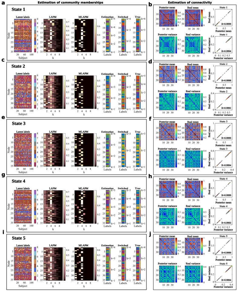
Fig. 2: Validation of group-level community memberships and connectivity estimates using synthetic fMRI data with 10dB. The left panels (a, c, e, g, and i) show the Bayesian estimates of individual-level and group-level latent community labels. Synthetic fMRI data for $100$ subjects and $35$ regions is generated by sampling a Gaussian distribution with a block covariance matrix (encoding the community structure), convolving the time series with a HRF, and adding Gaussian observation noise with a signal-to-noise ratio (SNR) of 10 dB. Five episodes with different communities are generated for each subject to simulate five brain states. The latent labels are first inferred separately for each subject and shown with different colors (left most matrices). The labels of all subjects are then taken together for the group-level analysis, where an LAPM is estimated from a Dirichlet posterior density. Each row of the matrix represents the probabilities of a node assigned to specific communities. Only the largest probability in each row of the LAPM is retained in the MLAPM, where the column index corresponds to the community memberships. The color bars indicate the community assignment probability in the LAPM and the MLAPM. The column indices in MLAPM are then turned into a vector of labels and a label-switching algorithm is applied. These estimates closely align with the true label vector used in the generative model, which is shown on the right most side of the left panels. The right panels (b, d, f, h, and j) show the Bayesian estimates of the posterior mean and variance connectivity matrices. The comparison between estimates and real values (posterior mean vs real mean and posterior variance vs real variance) is summarized in the scatter plots, where each point corresponds to a pair of nodes and $R$ is the correlation value.

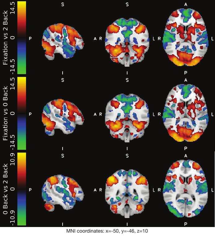
Fig. 2: Task activation maps (thresholded Z-MAX maps) for group analysis. Contrasts of 2-back vs fixation, 0-back vs fixation and 2-back vs 0-back for MNI coordinates (x = -50, y = -46, z = 10). For running 1st-level GLM-based FEAT (Woolrich et al., , 2001) in FSL, we added the confound predictors files released by HCP to the design matrix of the model for each individual. We then set up a 2nd-level design matrix for the contrast of 2-back, 0-back, and fixation. For the 3rd-level (the group-level GLM analysis (Woolrich et al., , 2004)), we applied cluster-wise inference and set up the cluster defining threshold (CDT) to be $Z=3.1$ ($P=0.001$) to avoid cluster failure problems as described in (Eklund et al., , 2016), with a family-wise error-corrected threshold of $P=0.05$. Maps are viewed by looking upward from the feet of the subject and the coordinate directions are denoted as Anterior (A), Posterior (P), Superior (S), Inferior (I), Left (L), and Right (R) (This figure was provided as a supplementary information in our previous work in Bian et al., (2021)).

To estimate the community memberships of a specific state from a single subject, a Markov chain of latent label vectors is generated using the MCMC allocation sampler and the samples are drawn from the posterior distribution after convergence of the Markov chain, by which Monte Carlo estimation is calculated. At the group level, categorical-Dirichlet conjugate pairs are used to model the latent labels in $\bm{Z}$ estimated at the individual level as described in the Methods section. The latent labels estimated for five states corresponding to five segments of synthetic fMRI time series from 100 virtual subjects are shown on the leftmost panels in Fig.2 (a, c, e, g, and i). A row ($\bm{z}_{i}$) represents the labels of 100 subjects for a specific node, and a column ($\bm{z}_{s}$) indicates the network labels of a subject.

At the group level, the latent labels are regarded as the observations of categorical-Dirichlet conjugate pair. An LAPM is estimated by drawing samples from a Dirichlet posterior density as shown in the second columns in the panel. Then an MLAPM containing the information of group-level community structure is constructed by retaining the maximum probability at each row of LAPM which represents the maximum probability of the node being assigned to a specific community. We then re-label the column index of the probability representing the most likely label assignment as a label vector of estimation. The estimation of community memberships by Bayesian hierarchical modelling have the label switching problem. To solve this problem, we apply a label-switching method (Nobile and Fearnside, , 2007, Wyse and Friel, , 2012) based on minimization of label vector distance and square assignment algorithm (Carpaneto and Toth, , 1980) to relabel the node to obtain a switched label vector as shown in the figures. See Bian et al., (2021) for further details and performance of the label-switching method in the context of a similar problem setting. The number of columns containing the maximum assignment probabilities indicates the number of communities at each state. We find that both the estimated community memberships and the numbers of columns for States 1 to 5 are largely consistent with the ground truth in the generative model.

Next, we model the individual-level adjacency matrices using the Normal-Normal-Inverse-Gamma (Normal-NIG) conjugate pair where the likelihood follows Normal distribution and the prior follows NIG distribution. We are interested in the mean and variance of the connectivity of a specific pair of nodes for 100 virtual subjects. We estimate the mean and variance of the connectivity by drawing the samples from the NIG posterior density (the estimated mean and variance of the connectivity are shown at the right panels in Fig.2 (b, d, f, h, and j). We compare the posterior samples with the real mean and variance of the connectivity between a specific pair of nodes $i$ and $j$ using 100 virtual subjects to validate the accuracy of the proposed generative model and the Bayesian inference algorithm. We found that the posterior samples of mean and variance were highly correlated with the real mean and variance as shown in the right most side of Fig.2. The color dots in the scatter plot are distributed into two groups for posterior samples of both mean and variance. This is because the elements $\gamma$ of the covariance matrix in the generative model that indicates intra-community couplings are sampled from $\gamma\sim U(0.8,1)$ and the elements $\omega$ indicating inter-community couplings are sampled from $\omega\sim U(0,0.2)$. The elements $\gamma$ and $\omega$ determine the density of blocks in the adjacency matrix which shows significant discrepancy between intra-community connectivity and inter-community connectivity.

4.2 Method evaluation using working memory task-fMRI data

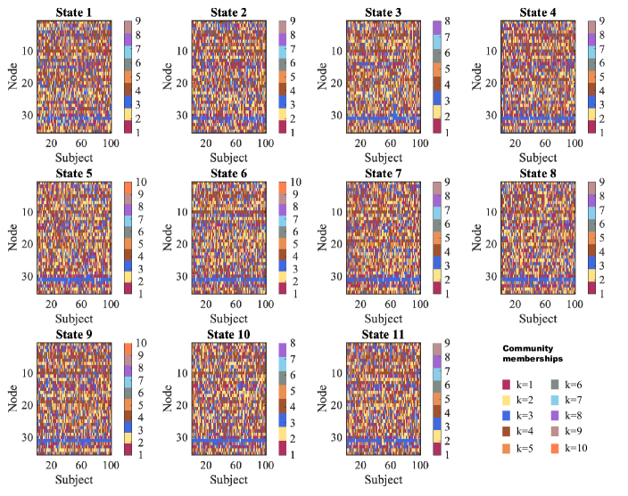
Fig. 3: Estimation of community memberships at individual level using working memory task-fMRI data. Different colors represent community memberships of functional brain networks from State 1 to 11 for 100 unrelated healthy subjects. The rows correspond to the nodes and the columns correspond to the subjects.

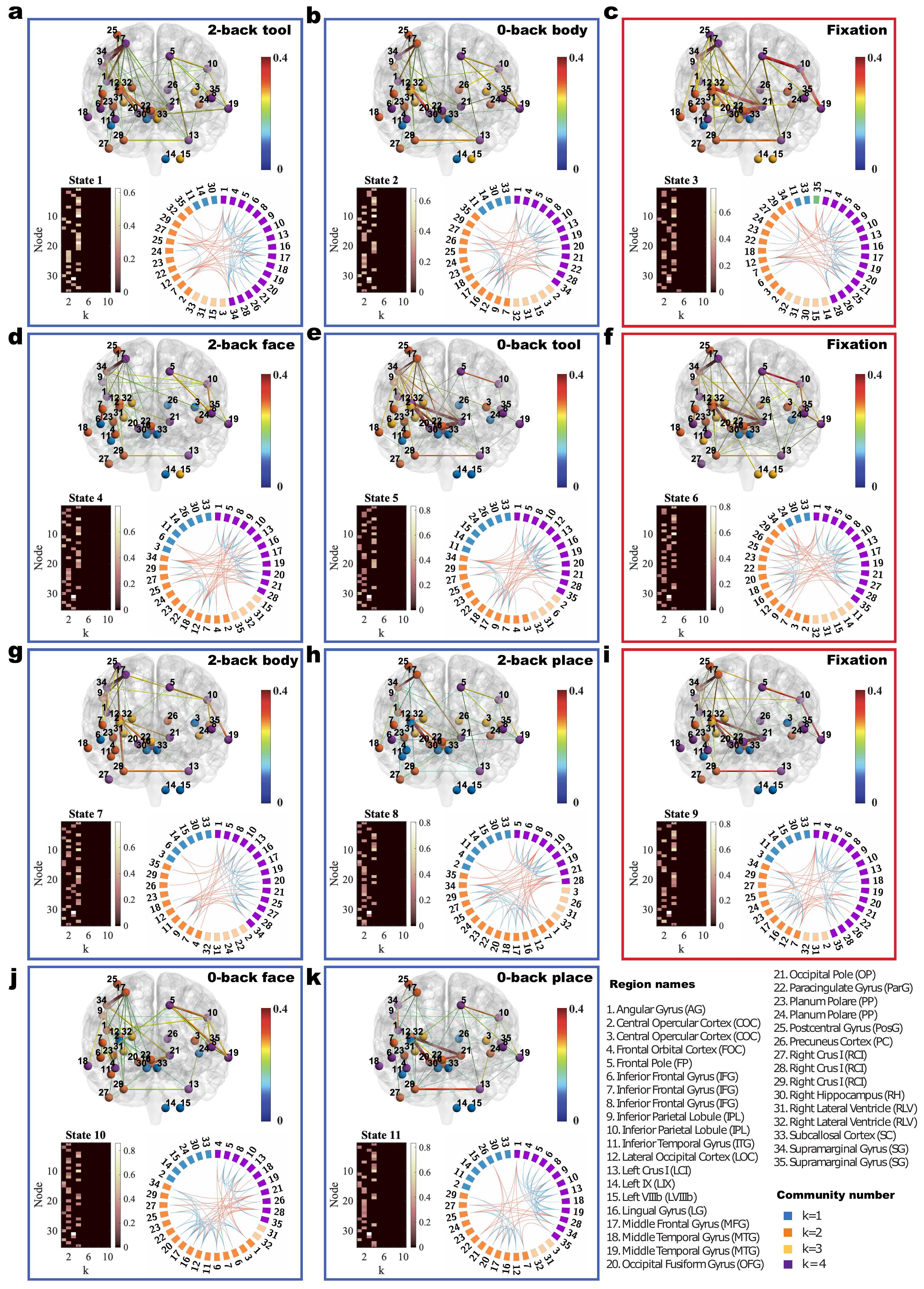
Fig. 4: Community structure of the discrete brain states estimated from group-level analysis using working memory task fMRI. The figures with blue frames represent brain states corresponding to working memory tasks (a 2-back tool; b 0-back body; d 2-back face; e 0-back tool; g 2-back body; h 2-back place; j 0-back face; and k 0-back place) and those with red frames represent brain states corresponding to fixation in c, f, and i. Each brain state shows connectivity at a sparsity level of 10%. The different colors of the labels represent community memberships which are the column indices in the MLAPM for each node. The strength of the connectivity is represented by the colors shown in the bar at the right of each frame. In Circos maps, nodes in the same community are adjacent and have the same color. Node numbers and abbreviations of the corresponding brain regions are shown around the circles. In each frame, different colors represent different community numbers. The connectivity above the sparsity level is represented by arcs. The blue links represent connectivity within communities and the red links represent connectivity between communities.

For real fMRI data analysis, we extracted the time series of 35 nodes whose MNI coordinates were determined by significant activations obtained via clusterwise inference using FSL (Smith et al., , 2004). We show the results of analysing the data from left-right phase encoding. The locations of the discrete brain states of State 1 (2-back tool), State 2 (0-back body), State 3 (fixation), State 4 (2-back face), State 5 (0-back tool), State 6 (fixation), State 7(2-back body), State 8 (2-back place), State 9 (fixation), State 10 (0-back face), and State 11 (0-back place) are illustrated in previous work (Bian et al., , 2021). The estimated labels (i.e., community memberships of the nodes) of individual-level analysis for 100 unrelated healthy subjects are shown in Fig.3. Different colors represent the community memberships $k$. The latent labels at the individual level are estimated via drawing latent label vector samples in a Markov chain generated from the posterior density $p(\bm{z}|\bm{x})$. These labels in Fig.3 are the estimation at the individual level and are considered as the observation at the group-level analysis. The estimates of community memberships and brain network connectivity at the group level are visualized in Fig.4. The group-level community structure is summarized by the MLAPM matrix, where the number of columns represents the estimated number of communities $K$ at the group level. The row index indicates the node number and the column index indicates the community memberships at the group level. The bar shows the value of the maximum assignment probability of the labels. The brain network connectivity is visualized using BrainNet Viewer (Xia et al., , 2013) and Circos. The community memberships of different states are inconsistent with each other due to the label-switching phenomenon. Here, we used the relabelling algorithm (Bian et al., , 2021) to reassign the labels across different states. The group-level weighted edges are at a sparsity level of 10%, which is the mean connectivity estimated by drawing samples from the posterior density $\mu_{ij}\sim\mathcal{N}(\xi_{s},\kappa_{s}^{2}\sigma_{ij}^{2})$, the details of which are illustrated in the Appendix. The color bar on the right shows the strength of the group-level weighted (mean) connectivity. It is clear from Fig.4 that nodes are clustered into communities with different connectivity densities within and between communities. We find that there are strong connections in communities $k$ = 2 and 4, and weak connections in communities $k$ = 1 and 3 for a majority of the states. The Circos map provides a different perspective on the community patterns of the brain states. We summarise the common group-level community pattern for specific working memory load or fixation in Table 1.

2-back						0-back						Fixation
Community	Node number					Community	Node number					Community	Node number
k=1	14	30				k=1	14	30	33			k=1	33
k=2	7	12	23	29		k=2	7	17	23	25	27	k=2	7	12	23	29
							29						34
k=3	31					k=3	31	32				k=3	31	32
k=4	5	8	10	13		k=4	5	8	10	13	28	k=4	1	4	5	8
	19	21	28										10	13	19	21
													28

Table 1: A table of group-level community detection for working memory task fMRI data. This table summarises the nodes commonly located in a specific community $k$ for all of the picture types in the working memory tasks.

The estimation of mean and variance connectivity for discrete brain states are shown in Fig.5a and b respectively. We found that the estimated connectivity patterns show subtle changes between different brain states. The mean adjacency matrix evaluates the averaged strength of the connectivity of the brain network and the variance adjacency matrix reflects the variability of the connectivity between subjects. Small changes to a largely stable latent FC patterns may be sufficient to give rise to a wide variety of cognitive and behavioural states (Lurie et al., , 2020).

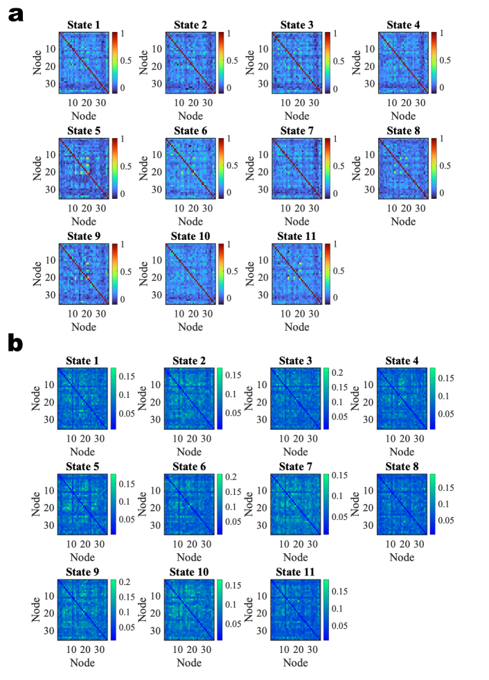
Fig. 5: Estimation of group-level FC. The estimated mean and variance connectivity matrices via hierarchical Bayesian modelling using working memory task fMRI data. a The estimated mean connectivity matrices of 35 nodes by drawing samples from the posterior density of Normal distribution. The bar represents the connectivity strength. b The estimated variance matrices by drawing samples from posterior density of NIG distribution with the bar showing the value of pairwise variance.

5 Discussion

In this work, we propose a new generative model to simulate synthetic fMRI data for validation of a multilayer community detection algorithm. The proposed generative model is simple to construct and contains the ground truth of the community memberships following categorical-Dirichlet distributions and the inter- and intra-connectivity densities following uniform distributions. The model characterizes a delay of neural responses via introducing a convolution with HRF.

We first discuss the group-level modelling of functional connectivity. Constructing group representative network by estimating a mean (group-averaged) functional connectivity (Bian et al., , 2021) ignores the variation of brain networks across individuals. Other methods that set a threshold to the functional connectivity (Achard et al., , 2006), may lose some important topological information about the networks. In this paper, the method based on hierarchical Bayesian modelling is able to characterize both averaged strength and inter-individual variation of weighted FC between brain regions across population. The method applies a Normal Normal-Inverse-Gamma (Normal-NIG) conjugate pair to the individual functional networks, by which a group-level mean and variance connectivity matrices are estimated by drawing samples from Normal and Inverse-Gamma posterior density respectively.

Next, we discuss the group-level modelling of community structure. The organization of functional brain networks is defined by the underlying community structure of these brain networks (Bassett et al., , 2011, 2013, Betzel et al., , 2018). Averaging over individual functional networks may ignore the differences and variations of community structure and inter- and intra-community connectivity densities with respect to individual functional networks. For community structure estimation, we propose the hierarchical Bayesian modelling based on LBM and MCMC sampling with absorption/ejection moves which are able to estimate latent labels with an unknown number of communities. This framework can not only identify the common community structure across individuals, but also evaluate the variability of the community structure patterns between individuals in contrast to the methods that only model the group-averaged FC. Furthermore, modelling the adjacency matrices of the group can evaluate both the mean and variance of functional connectivity, which reflects the average strength and variability of the brain regional interactions.

In this paper, we relax the assumption of fixing the number of communities $K$ and assumed it as a random variable that follows a Poisson distribution. We estimate the value of $K$, considering it a free parameter, via Bayesian inversion rather than using a model fitting strategy (Bian et al., , 2021). The absorption and ejection moves integrated into the Metroplis-Hastings sampler enables variation of $K$ in the constructed Markov chain, so that the samples of both $K$ and $\bm{z}$ can be drawn from the collapsed posterior density at the individual level. In this case, the inference of latent label vector $\bm{z}$ is not constrained by the pre-determined number of communities, which makes the estimates of labels at individual level more flexible compared to the method using a fixed value of $K$.

The samples generated by the MCMC sampler with the Gibbs and the M3 moves (Nobile and Fearnside, , 2007, Wyse and Friel, , 2012) typically got stuck in different local modes for different runs of MCMC simulation, which implies biased estimation, due to only a single observation (the group-averaged connectivity) being taken into account. Modelling the individual FC rather than the group-averaged FC provides insight into the variability of both the observations themselves, and the variability in the community structure between subjects, and can also alleviate the problem of the sampler getting stuck in a local mode. However, in the hierarchical Bayesian framework, the variability of the estimated latent labels at individual-level modelling results in variation in the sizes of the communities, which in turn results in variation in the sizes of the blocks in LBM at individual level. Therefore, we do not infer the block parameters $\bm{\pi}$ in the group-level functional brain networks in this paper.

The method proposed in this paper solves many of the problems illustrated in Bian et al., (2021). However, there are still some limitations of the current work. The multilayer community detection works well in synthetic fMRI networks with simulated communities where the connectivity is formed explicitly based on predefined known community structure. However, the communities are unknown in real functional brain networks. There is no standard algorithm for general community detection because the network architectures in real world are assumed to be generated from different latent generation processes. Community detection using LBM is based on the information of adjacency matrix which only measures the FC between pairs of nodes, but does not utilize the information of metadata or features on the nodes. Another work proposed by Hoffmann et al., (2020) detects communities in networks only using raw time series data on nodes without observing edges. Although treating node attributes or metadata as ground truth of community is used in many research works, a recent study shows that metadata are not the same as ground truth and that treating them as such induces significant theoretical and practical problems (Peel et al., , 2017). In future, finding the relationship between community detection and node metadata with respect to the network structure is worth exploring. Hierarchically modelling the group-level node metadata along with the multilayer FC is an interesting topic for future research.

In this paper, we have not utilized the assessment of neurological and behavioural function to examine the behavioural relevance of individual differences about the estimation of group-level community structure. In the future research, we plan to relate the HCP behavioural data such as the measures of mood, anxiety, substance abuse, personality, fluid intelligence, and sleep function, etc (Barch et al., , 2013) to the FC. Especially the connectivity metrics associated with hub (or rich clubs) by which we will be able to explain how variation in individual behaviour measurements relate to variations in functional brain networks.

Author contributions

Lingbin Bian: Conceptualization, Methodology, Data curation, Visualization, Software, Formal analysis, Investigation, Validation, Writing - original draft; Nizhuan Wang: Writing - review and editing; Leonardo Novelli: Writing - review and editing; Jonathan Keith: Conceptualization, Methodology, Investigation, Validation, Funding acquisition, Project administration; Resources; Supervision, Writing - review and editing; Adeel Razi: Conceptualization, Methodology, Investigation, Validation, Funding acquisition, Project administration, Resources, Supervision, Writing - review and editing.

Code availability

The code and analysis results for GLM (Shell script), hierarchical Bayesian modelling (MATLAB), and brain network visualization (MATLAB, Perl) are available at:
https://github.com/LingbinBian/HierarchicalBayesianModelling.

Appendix A The likelihood and posterior of group-level connectivity model

Likelihood: The likelihood of the group connectivity model is

$$p(\bm{X}_{ij}|\pi_{ij}) = \prod_{s=1}^{S}p(x_{ij}^{s}|\mu_{ij},\sigma_{ij}^{2})$$ (A.1)

$$= (2\pi\sigma_{ij}^{2})^{-S/2}\mbox{exp}\{-\frac{1}{2\sigma_{ij}^{2}}\sum_{s=l}^{S}(x_{ij}^{s}-\mu_{ij})^{2}\}$$

$$= (2\pi\sigma_{ij}^{2})^{-S/2}$$

$$\times\mbox{exp}\{-\frac{1}{2\sigma_{ij}^{2}}(\sum_{s=1}^{S}(x_{ij}^{s})^{2}-2\sum_{s=1}^{S}x_{ij}^{s}\mu_{ij}+\sum_{s=1}^{S}\mu_{ij}^{2})\}$$

$$= (2\pi\sigma_{ij}^{2})^{-S/2}\mbox{exp}\{-\frac{1}{2\sigma_{ij}^{2}}(q_{ij}-2\mu_{ij}w_{ij}+S\mu_{ij}^{2})\},$$

where $w_{ij}$ is the sum of the weights and $q_{ij}$ is the sum of squares of the weights in $\bm{X}_{ij}$.

Posterior: We derive the posterior of the model parameter $\pi_{ij}$ with prior $\mu_{ij}\sim\mathcal{N}(\xi,\kappa^{2}\sigma_{ij}^{2})$ and $\sigma_{ij}^{2}\sim\mbox{IG}(\nu/2,\rho/2)$ as follows.

$$p(\pi_{ij}|\bm{X}_{ij}) \propto p(\pi_{ij})p(\bm{X}_{ij}|\pi_{ij})$$ (A.2)

$$= p(\mu_{ij})p(\sigma_{ij}^{2})\prod_{s=1}^{S}p(x_{ij}^{s}|\mu_{ij},\sigma_{ij}^{2})$$

$$= (2\pi\kappa^{2}\sigma_{ij}^{2})^{-1/2}\mbox{exp}\{-\frac{1}{2\kappa^{2}\sigma_{ij}^{2}}(\mu_{ij}-\xi)^{2}\}$$

$$\times\frac{(\rho/2)^{\nu/2}}{\Gamma(\nu/2)}\sigma_{ij}^{-2(\nu/2+1)}\mbox{exp}\{-\rho/2\sigma_{ij}^{2}\}$$

$$\times(2\pi\sigma_{ij}^{2})^{-S/2}\mbox{exp}\{-\frac{1}{2\sigma_{ij}^{2}}(q_{ij}-2\mu_{ij}w_{ij}+S\mu_{ij}^{2})\}$$

$$= \frac{(\rho/2)^{\nu/2}}{\Gamma(\nu/2)}(2\pi\kappa^{2})^{-1/2}(2\pi)^{-S/2}\sigma_{ij}^{-1}\sigma_{ij}^{-\nu-2-S}$$

$$\times\mbox{exp}\{-\frac{1}{2\sigma_{ij}^{2}}[(\frac{1}{\kappa^{2}}+S)\mu_{ij}^{2}-2(\frac{1}{\kappa^{2}}\xi+w_{ij})\mu_{ij}$$

$$+\frac{1}{\kappa^{2}}\xi^{2}+q_{ij}+\rho]\}$$

The posterior of the Gaussian model is also a Normal-Inverse-Gamma distribution which can be denoted as $\mu_{ij}\sim\mathcal{N}(\xi_{s},\kappa_{s}^{2}\sigma_{ij}^{2})$ and $\sigma_{ij}^{2}\sim\mbox{IG}(\nu_{s}/2,\rho_{s}/2)$. The posterior density can be expressed as

$$p(\pi_{ij}|\bm{X}_{ij}) = (2\pi\kappa_{s}^{2}\sigma_{ij}^{2})^{-1/2}\mbox{exp}\{-\frac{1}{2\kappa_{s}^{2}\sigma_{ij}^{2}}(\mu_{ij}-\xi_{s})^{2}\}$$ (A.3)

$$\times\frac{(\rho_{s}/2)^{\nu_{s}/2}}{\Gamma(\nu_{s}/2)}\sigma_{ij}^{-2(\nu_{s}/2+1)}\mbox{exp}\{-\rho_{s}/2\sigma_{ij}^{2}\}$$

$$= \frac{(\rho_{s}/2)^{\nu_{s}/2}}{\Gamma(\nu_{s}/2)}(2\pi\kappa_{s}^{2})^{-1/2}\sigma_{ij}^{-1}\sigma_{ij}^{-\nu_{s}-2}$$

$$\times\mbox{exp}\{-\frac{1}{2\sigma_{ij}^{2}}(\frac{1}{\kappa_{s}^{2}}\mu_{ij}^{2}-\frac{2\xi_{s}}{\kappa_{s}^{2}}\mu_{ij}+\frac{\xi_{s}^{2}}{\kappa_{s}^{2}}+\rho_{s})\}.$$

Comparing the terms and coefficients with respect to $\mu_{ij}^{2}$, $\mu_{ij}$ and $\sigma_{ij}^{2}$,

$$-\nu_{s}-2=-\nu-2-S,$$ (A.4)

$$\frac{1}{\kappa_{s}^{2}}=\frac{1}{\kappa^{2}}+S,$$ (A.5)

$$\frac{2\xi_{s}}{\kappa_{s}^{2}}=2(\frac{1}{\kappa^{2}}\xi+w_{ij}),$$ (A.6)

$$\frac{\xi_{s}^{2}}{\kappa_{s}^{2}}+\rho_{s}=\frac{1}{\kappa^{2}}\xi^{2}+q_{ij}+\rho.$$ (A.7)

In summary, the parameters of the posterior density are given by

$$\nu_{s}=\nu+S,$$ (A.8)

$$\kappa_{s}^{2}=\frac{\kappa^{2}}{1+S\kappa^{2}},$$ (A.9)

$$\xi_{s}=\frac{\xi+w_{ij}\kappa^{2}}{1+S\kappa^{2}},$$ (A.10)

$$\rho_{s}=\frac{\xi^{2}}{\kappa^{2}}+q_{ij}+\rho-\frac{(\xi+w_{ij}\kappa^{2})^{2}}{1/\kappa^{2}+S}.$$ (A.11)

We can directly sample $\pi_{ij}$ from $\mbox{NIG}(\xi_{s},\kappa_{s}^{2}\sigma_{ij}^{2},\nu_{s}/2,\rho_{s}/2)$.

Supplementary information:
———————————————————————————————————————

		MNI coordinates			Voxel locations
Node number	Z-MAX	x	y	z	x	y	z	Region name
1	4.97	48	-58	22	21	34	47	Angular Gyrus
2	9.61	36	8	12	27	67	42	Central Opercular Cortex
3	8.27	-36	4	12	63	65	42	Central Opercular Cortex
4	6.48	40	34	-14	25	80	29	Frontal Orbital Cortex
5	7.83	-12	46	46	51	86	59	Frontal Pole
6	4.84	54	32	-4	18	79	34	Inferior Frontal Gyrus
7	6	52	38	10	19	82	41	Inferior Frontal Gyrus
8	4.38	-52	40	6	71	83	39	Inferior Frontal Gyrus
9	6.05	52	-70	36	19	28	54	Inferior Parietal Lobule PGp R
10	7.26	-48	-68	34	69	29	53	Inferior Parietal Lobule PGp L
11	6.18	44	-24	-20	23	51	26	Inferior Temporal Gyrus
12	9.54	36	-86	16	27	20	44	Lateral Occipital Cortex
13	8.04	-30	-80	-34	60	23	19	Left Crus I
14	7.6	-8	-58	-52	49	34	10	Left IX
15	6.9	-22	-48	-52	56	39	10	Left VIIIb
16	14.5	6	-90	-10	42	18	31	Lingual Gyrus
17	10.3	30	10	58	30	68	65	Middle Frontal Gyrus
18	6.61	66	-30	-12	12	48	30	Middle Temporal Gyrus
19	4.53	-68	-34	-4	79	46	34	Middle Temporal Gyrus
20	14.5	18	-88	-8	36	19	32	Occipital Fusiform Gyrus
21	5.06	-12	-92	-2	51	17	35	Occipital Pole
22	9.87	6	40	-6	42	83	33	Paracingulate Gyrus
23	12	42	-16	-2	24	55	35	Planum Polare
24	11.3	-40	-22	0	65	52	36	Planum Polare
25	9.03	38	-26	66	26	50	69	Postcentral Gyrus
26	8.31	-10	-60	14	50	33	43	Precuneus Cortex
27	5.7	46	-60	-42	22	33	15	Right Crus I
28	8.34	32	-80	-34	29	23	19	Right Crus I
29	10.9	32	-58	-34	29	34	19	Right Crus I
30	6.41	10	-8	-14	40	59	29	Right Hippocampus
31	6.19	32	-52	2	29	37	37	Right Lateral Ventricle
32	7.69	24	-46	16	33	40	44	Right Lateral Ventricle
33	6.13	0	10	-14	45	68	29	Subcallosal Cortex
34	10.7	48	-44	46	21	41	59	Supramarginal Gyrus
35	4.23	-50	-46	10	70	40	41	Supramarginal Gyrus

Table 1: Significant activations of cluster wise inference (cluster-corrected Z>3.1, P<0.05). Activations are described in terms of local maximum Z (Z-MAX) statistic within each cluster including the activations of all contrast maps among 2-back, 0-back, and fixation. (Bian et al., , 2021)

References

- Achard et al., (2006) Achard, S., Salvador, R., Whitcher, B., Suckling, J., and Bullmore, E. (2006). A resilient, low-frequency, small-world human brain functional network with highly connected association cortical hubs. Journal of Neuroscience, 26(1):63–72.
- Allen et al., (2014) Allen, E. A., Damaraju, E., Plis, S. M., Erhardt, E. B., Eichele, T., and Calhoun, V. D. (2014). Tracking whole-brain connectivity dynamics in the resting state. Cerebral Cortex, 24:663–676.
- Aquino et al., (2020) Aquino, K. M., Fulcher, B. D., Parkes, L., Sabaroedin, K., and Fornito, A. (2020). Identifying and removing widespread signal deflections from fMRI data: Rethinking the global signal regression problem. NeuroImage, 212(February):116614.
- Barch et al., (2013) Barch, D. M., Burgess, G. C., Harms, M. P., Petersen, S. E., Schlaggar, B. L., Corbetta, M., Glasser, M. F., Curtiss, S., Dixit, S., Feldt, C., Nolan, D., Bryant, E., Hartley, T., Footer, O., Bjork, J. M., Poldrack, R., Smith, S., Johnsen-Berg, H., Snyder, A. Z., Van Essen, D. C., and for the WU-Minn HCP Consortium (2013). Function in the human connectome: Task-fMRI and individual differences in behavior. NeuroImage, 80:169–189.
- Bassett et al., (2013) Bassett, D. S., Porter, M. A., Wymbs, N. F., Grafton, S. T., Carlson, J. M., and Mucha, P. J. (2013). Robust detection of dynamic community structure in networks. CHAOS, 23:13142.
- Bassett et al., (2011) Bassett, D. S., Wymbs, N. F., Porter, M. A., Mucha, P. J., Carlson, J. M., and Grafton, S. T. (2011). Dynamic reconfiguration of human brain networks during learning. PNAS, 108(18):7641–7646.
- Betzel et al., (2019) Betzel, R. F., Bertolero, M. A., Gordon, E. M., Gratton, C., Dosenbach, N. U., and Bassett, D. S. (2019). The community structure of functional brain networks exhibits scale-specific patterns of inter- and intra-subject variability. NeuroImage, 202(September 2018):115990.
- Betzel et al., (2018) Betzel, R. F., Medaglia, J. D., and Bassett, D. S. (2018). Diversity of meso-scale architecture in human and non-human connectomes. Nature Communications, 9(1).
- Bian et al., (2020) Bian, L., Cui, T., Sofronov, G., and Keith, J. (2020). Network structure change point detection by posterior predictive discrepancy. In Monte Carlo and Quasi-Monte Carlo Methods, MCQMC 2018, Rennes, France, July 1–6, pages 107–123. Springer proceedings in Mathematics & Statistics.
- Bian et al., (2021) Bian, L., Cui, T., Thomas Yeo, B., Fornito, A., Razi, A., and Keith, J. (2021). Identification of community structure-based brain states and transitions using functional MRI. NeuroImage, 244(September):118635.
- Calhoun et al., (2014) Calhoun, V. D., Miller, R., Pearlson, G., and Adali, T. (2014). The chronnectome: Time-varying connectivity networks as the next frontier in fMRI data discovery. Neuron, 84(2):262–274.
- Carpaneto and Toth, (1980) Carpaneto, G. and Toth, P. (1980). Algorithm 548: Solution of the assignment problem [H]. ACM Transactions on Mathematical Software (TOMS), 6(1):104–111.
- Cribben et al., (2012) Cribben, I., Haraldsdottir, R., Atlas, L. Y., Wager, T. D., and Lindquist, M. A. (2012). Dynamic connectivity regression: determining state-related changes in brain connectivity. NeuroImage, 61:720–907.
- Cribben and Yu, (2017) Cribben, I. and Yu, Y. (2017). Estimating whole-brain dynamics by using spectral clustering. Journal of the Royal Statistical Society. Series C (Applied Statistics), 66:607–627.
- Deco et al., (2008) Deco, G., Jirsa, V. K., Robinson, P. A., Breakspear, M., and Friston, K. (2008). The dynamic brain: From spiking neurons to neural masses and cortical fields. PLoS Computational Biology, 4(8).
- Eklund et al., (2016) Eklund, A., Nichols, T. E., and Knutsson, H. (2016). Cluster failure: Why fMRI inferences for spatial extent have inflated false-positive rates. PNAS, 113(28):7900–7905.
- Friston et al., (2021) Friston, K. J., Fagerholm, E. D., Zarghami, T. S., Parr, T., Hipólito, I., Magrou, L., and Razi, A. (2021). Parcels and particles: Markov blankets in the brain. Network Neuroscience, 0(ja):1–76.
- Friston et al., (2014) Friston, K. J., Kahan, J., Biswal, B., and Razi, A. (2014). A DCM for resting state fMRI. NeuroImage, 94:396–407.
- Gonzalez-Castillo and Bandettini, (2018) Gonzalez-Castillo, J. and Bandettini, P. A. (2018). Task-based dynamic functional connectivity: Recent findings and open questions. NeuroImage, 180(August 2017):526–533.
- Hastings, (1970) Hastings, W. (1970). Monte Carlo sampling methods using Markov chains and their applications. Biometrika, 57(1):97–109.
- Hoffmann et al., (2020) Hoffmann, T., Peel, L., Lambiotte, R., and Jones, N. S. (2020). Community detection in networks without observing edges. Science Advances, 6(4):1–12.
- Hutchison et al., (2013) Hutchison, R. M., Womelsdorf, T., Allen, E. A., Bandettini, P. A., Calhoun, V. D., Corbetta, M., Penna, S. D., Duyn, J. H., Glover, G. H., Gonzalez-castillo, J., Handwerker, D. A., Keilholz, S., Kiviniemi, V., Leopold, D. A., Pasquale, F. D., Sporns, O., Walter, M., and Chang, C. (2013). Dynamic functional connectivity : Promise , issues , and interpretations. NeuroImage, 80:360–378.
- Jirsa et al., (2010) Jirsa, V. K., Sporns, O., Breakspear, M., Deco, G., and McIntosh, A. R. (2010). Towards the virtual brain: network modeling of the intact and the damaged brain. Archives Italiennes de Biologie, 148:189–205.
- Kringelbach and Deco, (2020) Kringelbach, M. L. and Deco, G. (2020). Brain states and transitions: Insights from computational neuroscience. Cell Reports, 32(10):108128.
- Lehmann et al., (2021) Lehmann, B. C., Henson, R. N., Geerligs, L., Cam-CAN, and White, S. R. (2021). Characterising group-level brain connectivity: A framework using Bayesian exponential random graph models. NeuroImage, 225:117480.
- Lurie et al., (2020) Lurie, D. J., Kessler, D., Bassett, D. S., Betzel, R. F., Breakspear, M., Kheilholz, S., Kucyi, A., Liégeois, R., Lindquist, M. A., McIntosh, A. R., Poldrack, R. A., Shine, J. M., Thompson, W. H., Bielczyk, N. Z., Douw, L., Kraft, D., Miller, R. L., Muthuraman, M., Pasquini, L., Razi, A., Vidaurre, D., Xie, H., and Calhoun, V. D. (2020). Questions and controversies in the study of time-varying functional connectivity in resting fMRI. Network Neuroscience, 4(1):30–69.
- MacDaid et al., (2012) MacDaid, A., Murphy, T. B., Friel, N., and Hurley, N. (2012). Improved Bayesian inference for the stochastic block model with application to large networks. Computational Statistics and Data Analysis, 60:12–31.
- Metropolis et al., (1953) Metropolis, N., Rosenbluth, A. W., Rosenbluth, M. N., Teller, A. H., and Teller, E. (1953). Equation of state calculations by fast computing machines. The Journal of Chemical Physics, 21(6):1087–1092.
- Monti et al., (2017) Monti, R. P., Lorenz, R., Braga, R. M., Anagnostopoulos, C., Leech, R., and Montana, G. (2017). Real-time estimation of dynamic functional connectivity networks. Human Brain Mapping, 38(1):202–220.
- Nobile and Fearnside, (2007) Nobile, A. and Fearnside, A. T. (2007). Bayesian finite mixtures with an unknown number of components: The allocation sampler. Statistics and Computing, 17:147–162.
- Park and Friston, (2013) Park, H.-J. and Friston, K. (2013). Structural and functional brain networks: From connections to cognition. Science, 342(6158).
- Parkes et al., (2018) Parkes, L., Fulcher, B., Yücel, M., and Fornito, A. (2018). An evaluation of the efficacy, reliability, and sensitivity of motion correction strategies for resting-state functional MRI. NeuroImage, 171(December 2017):415–436.
- Pavlović et al., (2020) Pavlović, D. M., Guillaume, B. R., Towlson, E. K., Kuek, N. M., Afyouni, S., Vértes, P. E., Thomas Yeo, B., Bullmore, E. T., and Nichols, T. E. (2020). Multi-subject Stochastic Blockmodels for adaptive analysis of individual differences in human brain network cluster structure. NeuroImage, page 116611.
- Peel et al., (2017) Peel, L., Larremore, D. B., and Clauset, A. (2017). The ground truth about metadata and community detection in networks. Science Advances, 3(5):1–9.
- Power et al., (2017) Power, J. D., Plitt, M., Laumann, T. O., and Martin, A. (2017). Sources and implications of whole-brain fMRI signals in humans. NeuroImage, 146(September 2016):609–625.
- Razi and Friston, (2016) Razi, A. and Friston, K. J. (2016). The connected brain: Causality, models, and intrinsic dynamics. IEEE Signal Processing Magazine, 26(5):340–343.
- Razi et al., (2015) Razi, A., Kahan, J., Rees, G., and Friston, K. J. (2015). Construct validation of a DCM for resting state fMRI. NeuroImage, 106:1–14.
- Razi et al., (2017) Razi, A., Seghier, M. L., Zhou, Y., McColgan, P., Zeidman, P., Park, H.-J., Sporns, O., Rees, G., and Friston, K. J. (2017). Large-scale DCMs for resting-state fMRI. Network Neuroscience, 1(4):381–414.
- Robinson et al., (2015) Robinson, L. F., Atlas, L. Y., and Wager, T. D. (2015). Dynamic functional connectivity using state-based dynamic community structure: Method and application to opioid analgesia. NeuroImage, 108:274–291.
- Smith et al., (2004) Smith, S. M., Jenkinson, M., Woolrich, M. W., Beckmann, C. F., Behrens, T. E., Johansen-Berg, H., Bannister, P. R., Luca, M. D., Drobnjak, I., Flitney, D. E., Niazy, R. K., Saunders, J., Vickers, J., Zhang, Y., Stefano, N. D., Brady, J. M., and Matthews, P. M. (2004). Advances in functional and structural MR image analysis and implementation as FSL. NeuroImage, 23:S208–S219.
- Smith et al., (2011) Smith, S. M., Miller, K. L., Salimi-Khorshidi, G., Webster, M., Beckmann, C. F., Nichols, T. E., Ramsey, J. D., and Woolrich, M. W. (2011). Network modelling methods for FMRI. NeuroImage, 54(2):875–91.
- Taghia et al., (2018) Taghia, J., Cai, W., Ryali, S., Kochalka, J., Nicholas, J., Chen, T., and Menon, V. (2018). Uncovering hidden brain state dynamics that regulate performance and decision-making during cognition. Nature Communications, 9(1).
- Ting et al., (2021) Ting, C. M., Samdin, S. B., Tang, M., and Ombao, H. (2021). Detecting dynamic community structure in functional brain networks across individuals: A multilayer approach. IEEE Transactions on Medical Imaging, 40(2):468–480.
- Van Essen et al., (2013) Van Essen, D. C., Smith, S. M., Barch, D. M., Behrens, T. E., Yacoub, E., and Ugurbil, K. (2013). The WU-Minn Human Connectome Project: An overview. NeuroImage, 80:62–79.
- Vidaurre et al., (2018) Vidaurre, D., Abeysuriya, R., Becker, R., Quinn, A. J., Alfaro-Almagro, F., Smith, S. M., and Woolrich, M. W. (2018). Discovering dynamic brain networks from big data in rest and task. NeuroImage, 180(June 2017):646–656.
- Woolrich et al., (2004) Woolrich, M. W., Behrens, T. E., Beckmann, C. F., Jenkinson, M., and Smith, S. M. (2004). Multilevel linear modelling for FMRI group analysis using Bayesian inference. NeuroImage, 21(4):1732–1747.
- Woolrich et al., (2001) Woolrich, M. W., Ripley, B. D., Brady, M., and Smith, S. M. (2001). Temporal autocorrelation in univariate linear modeling of FMRI data. NeuroImage, 14(6):1370–1386.
- Wyse and Friel, (2012) Wyse, J. and Friel, N. (2012). Block clustering with collapsed latent block models. Statistics and Computing, 22:415–428.
- Xia et al., (2013) Xia, M., Wang, J., and He, Y. (2013). BrainNet viewer: A network visualization tool for human brain connectomics. PLoS ONE, 8(7).

References

- Bian et al., (2021) Bian, L., Cui, T., Thomas Yeo, B., Fornito, A., Razi, A., and Keith, J. (2021). Identification of community structure-based brain states and transitions using functional MRI. NeuroImage, 244(September):118635.
- Eklund et al., (2016) Eklund, A., Nichols, T. E., and Knutsson, H. (2016). Cluster failure: Why fMRI inferences for spatial extent have inflated false-positive rates. PNAS, 113(28):7900–7905.
- Woolrich et al., (2004) Woolrich, M. W., Behrens, T. E., Beckmann, C. F., Jenkinson, M., and Smith, S. M. (2004). Multilevel linear modelling for FMRI group analysis using Bayesian inference. NeuroImage, 21(4):1732–1747.
- Woolrich et al., (2001) Woolrich, M. W., Ripley, B. D., Brady, M., and Smith, S. M. (2001). Temporal autocorrelation in univariate linear modeling of FMRI data. NeuroImage, 14(6):1370–1386.