ViT-AE++: Improving Vision Transformer Autoencoder for Self-supervised Medical Image Representations

Abstract

Self-supervised learning has attracted increasing attention as it learns data-driven representation from data without annotations. Vision transformer-based autoencoder (ViT-AE) [He et al. (2021)] is a recent self-supervised learning technique that employs a patch-masking strategy to learn a meaningful latent space. In this paper, we focus on improving ViT-AE (nicknamed ViT-AE$+$$+$) for a more effective representation of both 2D and 3D medical images. We propose two new loss functions to enhance the representation during the training stage. The first loss term aims to improve self-reconstruction by considering the structured dependencies and hence indirectly improving the representation. The second loss term leverages contrastive loss to directly optimize the representation from two randomly masked views. As an independent contribution, we extended ViT-AE$+$$+$ to a 3D fashion for volumetric medical images. We extensively evaluate ViT-AE$+$$+$ on both natural images and medical images, demonstrating consistent improvement over vanilla ViT-AE and its superiority over other contrastive learning approaches. Our code is available at https://github.com/chinmay5/vit_ae_plus_plus.git

1 Introduction

Self-supervised representation learning (SSRL), especially recent contrastive learning-based methods [Chen et al. (2020), He et al. (2020), Oord et al. (2018)], is a promising technique that can learn informative data representations from data without labels. It is particularly useful and relevant in medical imaging, where labeled data are often scarce for traditional supervised training and the high cost of manual labeling that relies on domain knowledge.

Contrastive learning-based approaches aim to attract similar image pairs and rebuff dissimilar image pairs. A similar image pair can be generated by two augmented views of one image, and the other image samples can be used to construct dissimilar image pairs. In medical imaging, SSRL are mainly used for two purposes: 1) pre-training deep networks for transfer learning or for network initialization [Zhou et al. (2019), Chaitanya et al. (2020), Zeng et al. (2021)], 2) extracting meaningful information from data [Li et al. (2021), Dufumier et al. (2021)] which is the downstream task for applying SSRL in this work.

As opposed to contrastive learning, the recent vision transformer autoencoder (ViT-AE) approach [He et al. (2021)] is different from the above methods in principle. It randomly masks the sequential image patches and learns to reconstruct the original image using an autoencoder and vision transformer-based architecture. They demonstrate that such a simple reconstruction can facilitate the vision transformer to learn effective image representations in a self-supervised fashion. Although ViT-AE achieves promising results in the natural image domain, we argue that two components of this framework could be further optimized.

First, in the vanilla ViT-AE pipeline, it computes pixel-wise reconstruction loss of the autoencoder and does not consider structured dependencies of the reconstruction, which might limit to capture of semantic features. For example, medical images contain rich texture and morphology, such structural information across pixels is important to complement traditional pixel-wise reconstruction (often with a $\mathcal{L}$-2 norm loss).

Second, since the representation is indirectly learned by a self-reconstruction via an autoencoder, there might be room to optimize the target representation directly. For example, contrastive learning-based methods [Chen and He (2021), Chen et al. (2020)] straightforwardly match the target representation from two augmented views.

Contributions.

(1) We introduce an auxiliary reconstruction task that considers structural dependencies to complement the pixel-wise reconstruction. (2) We unite two paradigms of contrastive learning-based and autoencoder-based methods and enjoy the benefits of both. (3) In extensive experiments, we demonstrate that both 2D and 3D ViT-AE$+$$+$ outperform the vanilla ViT-AE and its superiority over other contrastive learning approaches, setting up a strong baseline for learning self-supervised medical image representation.

2 Related Work

We mainly discuss prior works that are related to the technical contributions of ViT-AE$+$$+$.

Auxiliary loss functions.

In image segmentation tasks, auxiliary losses can regularize network training by serving as ‘deep supervision’ [Lee et al. (2015), Zhao et al. (2017)]. Liu et al. (2021) introduce a generic perceptual loss for dense prediction tasks. They argue that leveraging an auxiliary task that considers structural dependency can benefit various dense prediction tasks. Inspired by this work, we introduce an auxiliary reconstruction task to the autoencoder. In addition to perceptual loss, we develop a new edge-aware loss considering the richness of texture in medical images.

Contrastive loss.

Contrastive loss, such as SimCLR Chen et al. (2020) directly optimizes the image representation by maximizing the agreement between two augmented views. The asymmetric networks such as SimSiam Chen and He (2020) and BYOL Grill et al. (2020) follow a similar idea but only make use of positive pairs with two shared encoders. Considering the training efficiency, we borrow the loss design from SimSiam Chen and He (2020). Differently, we not only use random augmentation but also random masking to obtain hard training samples, analogous to random cropping in CNN-based backbone.

3 Method

Overview.

The objective is to learn a good domain-specific representation of 3D volumes using an autoencoder without labels. Consider an autoencoder with encoder ${E}$, decoder ${D}$, and a function $m(\cdot)$ for masking input patches in a vision transformer architecture. Given an image volume $X$, it is decomposed into $k$ sequential patches with a size of $n$$\times$n$\times$$n$. Then a random mask is applied on the sequential input patches to mask away $p$% of the patches. The remaining visible patches are referred to as $X^{*}$. The visible patches $X^{*}$ are fed to the encoder ${E}$ to extract features. For each missing patch, a token with 3D positional encoding is assigned to indicate the presence of such patches (called MASK tokens). The features of the visible patches along with MASK tokens are passed to the decoder. The decoder ${G}$ predicts image intensities for these MASK tokens and thereby reconstructs the whole volume, i.e., $X\approx{D}({E}(X^{*}))$. We introduce an auxiliary reconstruction task with a compound loss function $\mathcal{L}_{per}+\mathcal{L}_{edge}$ as shown in Fig. 1. The new loss is designed to capture high-order properties to complement the pixel-wise loss. To further enhance the target representation, we adopt contrastive loss to maximize the agreement from two random masked views. Fig. 1 shows the schematic view of our architecture. In the following sections, we explain each component in detail.

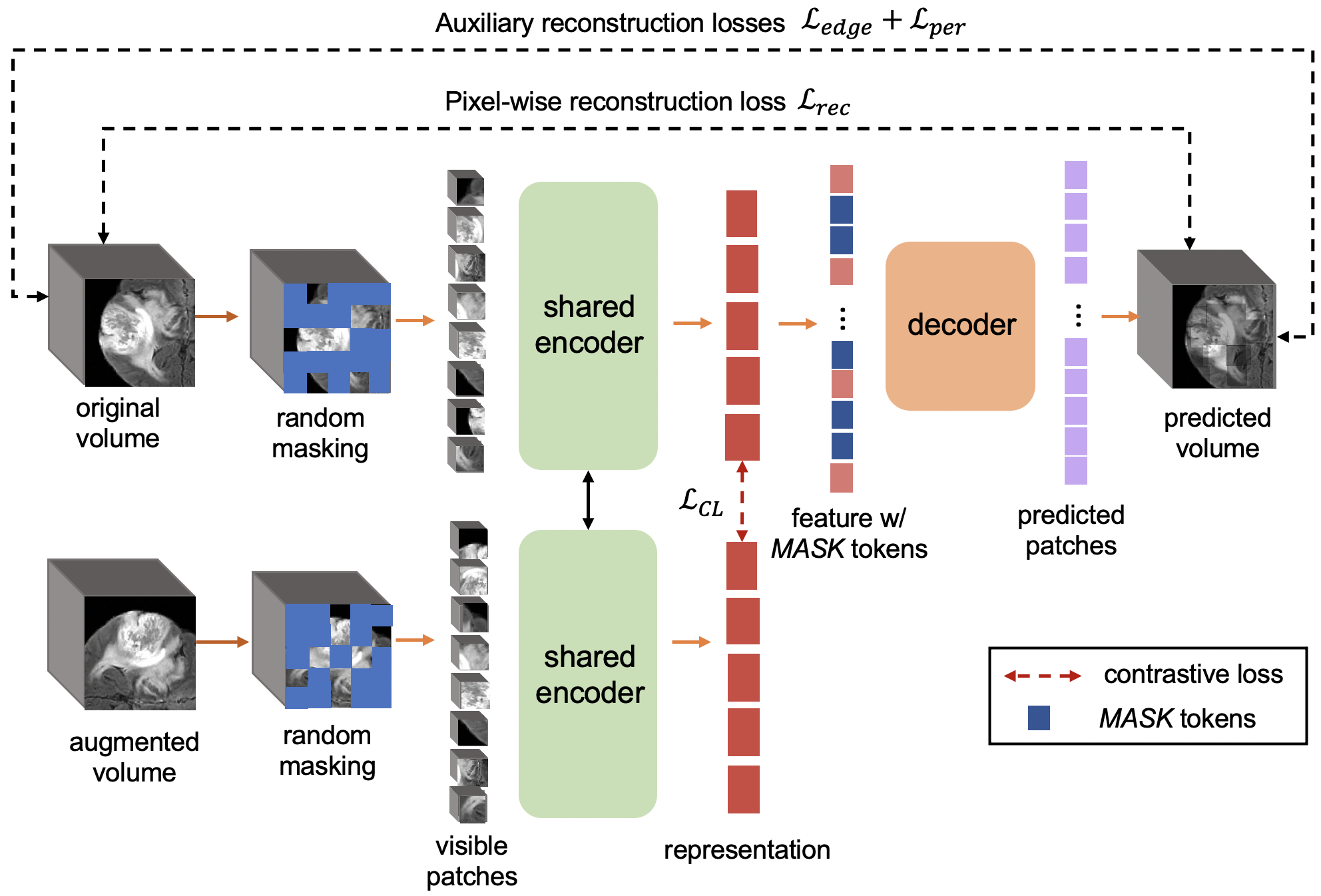
Figure 1: Our proposed ViT-AE++ framework. The upper half shows the training procedure of the autoencoder. An MRI volume is parsed and masked randomly and the visible patches are passed through to the encoder. Placeholder tokens for the masked patches are introduced after the encoder (referred to as the MASK tokens). The full set of encoded features and these placeholder tokens are passed to a decoder which reconstructs the whole MRI volume. We use a pixel-wise reconstruction loss and an auxiliary loss that concerns perceptual features (Eq. 1) and edge map (Eq. 2). The lower half demonstrates the optimization with a contrastive loss which is based on two randomly augmented and masked views. The representations from the two views are matched with cosine similarity loss (Eq. 3).

Vanilla ViT-AE with pixel-wise loss.

ViT-AE takes partial observations and reconstructs the original input. A random masking strategy is used to mask $p$% of the input volume. Notably, $p$ is a hyperparameter which will be discussed in a later section. The visible patches $X^{*}$ are fed through encoder ${E}$. The decoder ${D}$ reconstructs $X$ from ${E}(X^{*})$ using a mean-squared-error loss: $\mathcal{L}_{rec}=||{X}-{D}({E}(X^{*})||_{2}$.

Auxiliary compound loss.

Original ViT-AE uses the pixel-wise loss for training as mentioned above. In the medical image domain, perceptual features and edges encode meaningful semantics signals Shen et al. (2017). We employ a compound loss with deep high-level features and low-level edge-based features to enforce the network to use this supervision signal during training.

To exact deep multi-level features, we introduce VGG-based perceptual loss Johnson et al. (2016) to compute the feature similarity at multiple levels over $n$ 2D slices of one volume.

$$\mathcal{L}_{per}=\sum_{i=0}^{n}||VGG(x_{i})-VGG(\hat{x_{i}})||_{2}$$ (1)

where $VGG(\cdot)$ denotes multi-level features from the pre-trained VGG network using the same layers in (Johnson et al., 2016). $x_{i}$ and $\hat{x_{i}}$ denote the input image and the reconstructed image, respectively.

For low-level features, a 3D Sobel filter function Kanopoulos et al. (1988) $Sobel(\cdot)$ is used to compute the gradients from three directions. Firstly, the input volume is convolved with a fixed Sobel filter to generate gradients in the axial, coronal, and sagittal directions. The norm of these gradients is the edge map representation (Eq. 2). Please see the details in the Appendix.

The edge loss between original volume $X$ and the reconstruction $\hat{X}$ is formulated as:

$$\mathcal{L}_{edge}=||\emph{Sobel}(X)-\emph{Sobel}(\hat{X})||_{2}$$ (2)

Contrastive loss.

Along with the self-reconstruction, a contrastive loss is further introduced to enhance the target representation. It tries to match the feature representations between the two views of visible patches, denoted as $f_{1}$ and $f_{2}$. We used negative cosine distance as the loss function and the ‘stopping gradient’ optimization in Chen and He (2020).

$$\mathcal{L}_{CL}=-\frac{f_{1}}{\left\|f_{1}\right\|_{2}}\cdot\frac{{f_{2}}}{\left\|f_{2}\right\|_{2}},$$ (3)

ViT-AE$+$$+$.

The final optimization objective of ViT-AE$+$$+$ is

$$L=\mathcal{L}_{rec}+\lambda_{1}\mathcal{L}_{per}+\lambda_{2}\mathcal{L}_{edge}+\mathcal{L}_{CL}.$$ (4)

where $\lambda_{1}$ and $\lambda_{2}$ are hyperparameters and initially set to 0.01 and 10 respectively considering the loss scale. $\lambda_{2}$ is decreased linearly to stabilize the training process. The motivation for the linear scaling and other hyperparameters are discussed in the Results section.

4 Experiment Setup

We evaluate ViT-AE$+$$+$ extensively on public natural and medical image datasets, focusing on 3D brain MRI datasets.

2D Datasets.

CIFAR-10, CIFAR-100 and Tiny Imagenet-100 Russakovsky et al. (2015) are popular natural datasets to benchmark representation learning methods. In addition, we evaluate our method on a 2D chest X-ray dataset Kermany et al. (2018). It consists of 5118 images for training, 119 for validation, and 626 for testing. The task is to identify pneumonia based on chest X-ray images. All images are resized to 224$\times$224 pixels.

3D Datasets.

To highlight the effectiveness of 3D ViT-AE$+$$+$, we performed experiments on two public 3D datasets: 1) a multi-center MRI dataset (BraTS) Menze et al. (2014); Bakas et al. (2018) including 326 patients with a brain tumor. 2) The Erasmus Glioma Database (EGD) van der Voort et al. (2021) which consists of 768 MRI scans. Both datasets include FLAIR, T1, T2, and T1-c with a uniform voxel size 1$\times$1$\times$1 mm³. We train individual models and evaluate on the two datasets separately. The effectiveness of the learned representations is evaluated on two down-stream classification tasks: a) For BraTS, discriminating high-grade and low-grade tumor, and b) for EGD, predicting isocitrate dehydrogenase (IDH) mutation status (0 or 1).

We use the segmentation masks for both datasets to get its centroid and generate a 3D bounding box of 96$\times$96$\times$96 to localize the tumor. If the bounding box exceeds the original volume, the out-of-box region is padded with background intensity. Four modalities are concatenated to serve as a multi-modal input. The intensity range of all image volumes was rescaled to [0, 255] to guarantee the success of intensity-based augmentations.

Architecture and training configuration.

In this sub-section, we explain each component in the architecture and the training settings in detail.

Encoder and decoder.

Working on only the visible patches allows the encoder to process a fraction of 3D volumes with less GPU memory. We extend a standard ViT Dosovitskiy et al. (2021) to be 3D architecture as the encoder. 3D patches are embedded using a linear projection with added positional encoding with 3D coordinates. 12 encoder blocks, each with an embedding dimension of 768, are used. The decoder reconstructs the volume using features from the encoder and the MASK tokens mentioned in Sec. 3. Each MASK token is a shared learned vector that indicates the presence of a missing patch to be predicted. We add 3D positional encoding to all the tokens for sequential prediction Devlin et al. (2019). The decoder is realized using 8 transformer blocks, each with an embedding dimension of 512. After training, we only use the encoder as a feature extractor. The 3D position encoding is shown in the Appendix.

End-to-end training of ViT-AE$+$$+$ with contrastive loss.

ViT-AE$+$$+$ is trained for 1000 epochs using AdamW optimizer Loshchilov and Hutter (2019) with 0.05 weight decay. The base learning rate is 1e-3. The learning rate is annealed using cosine decay Loshchilov and Hutter (2017). The batch size is set to 4, adjusted to maximize GPU memory with an Nvidia RTX 3090. We use 40 epochs for our warm-up schedule Goyal et al. (2018). Gamma correction, affine transform and Gaussian noise augmentations are used to generate the second ”view” of the input volume. The two views are randomly masked and passed through the shared encoder ${E}$. Features generated by the encoder are compared using their cosine similarity (Eq. 3).

Evaluation strategy, classifier, and metrics.

For the EGD dataset, since there are 307 unlabeled images, we pre-train on the unlabeled data and perform the downstream task on the labeled dataset. For the other 2D and 3D datasets, the training of the proxy task and the target downstream task use the same dataset.

For evaluation on BraTS and EGD datasets, we follow the standard strategy to evaluate the quality of the pre-trained representations by training a supervised linear support vector machine classifier on the training set and then evaluating it on the test set. We use the sensitivity, specificity and Area Under the Receiver Operating Characteristic Curve (AUC) as the evaluation metrics. We use stratified five-fold nested cross-validation to reduce selection bias and validate each model. In each fold, we randomly sample 80% subjects from each class as the training set and the remaining 20% for each class as the test set. Furthermore, 20% of training data is separated and used exclusively to optimize the hyper-parameters within each fold.

For evaluation on CIFAR-10, CIFAR-100, Tiny Imagenet-100, and chest X-ray datasets, we use the linear probing strategy He et al. (2021). The decoder module is discarded and encoder weights are frozen. Thus, the encoder acts as a feature extractor. A supervised linear classifier is trained on the frozen representations. We use the pre-defined train and test splits. 20 % of the training data is separated for hyper-parameter tuning. We report the classification accuracy for the test split for all the datasets.

5 Results

ViT-AE$++$ $vs.$ ViT-AE on 2D datasets.

To quantify the effectiveness of our proposed loss functions, we compare our method against the vanilla ViT-AE on CIFAR-10, CIFAR-100, Tiny Imagenet-100 and chest X-ray datasets. We use the linear probing evaluation protocol and report the classification accuracy on the test sets. Please note that the VGG-perceptual loss for three natural image datasets is not a pre-trained VGG but one with randomized weights. This is because we do not wish any supervised signals involved during the self-supervised training stage. Tab. 1 shows that the features learned using ViT-AE$++$ consistently perform better than their vanilla counterpart. It indicates that ViT-AE$++$ can serve as a strong baseline for both natural and medical image domains.

Table 1: Comparison of ViT-AE$++$ and ViT-AE on four 2D datasets. We can observe consistent improvements in classification accuracy, benefiting from the new loss functions.

Method	CIFAR-10	CIFAR-100	Tiny ImageNet-100	chest X-ray
ViT-AE	94.10	75.61	70.42	95.20
ViT-AE++ (ours)	95.40	78.82	72.09	95.60

ViT-AE$++$ $vs.$ other methods on 3D datasets.

To focus on 3D medical image representation on small-scale datasets, we further evaluate the 3D version of ViT-AE$++$ and compare it with other state-of-the-art self-supervised methods (especially contrastive learning-based ones) on two classification tasks: a) discrimination of low-grade and high-grade brain tumors and b) prediction of IDH mutation status.

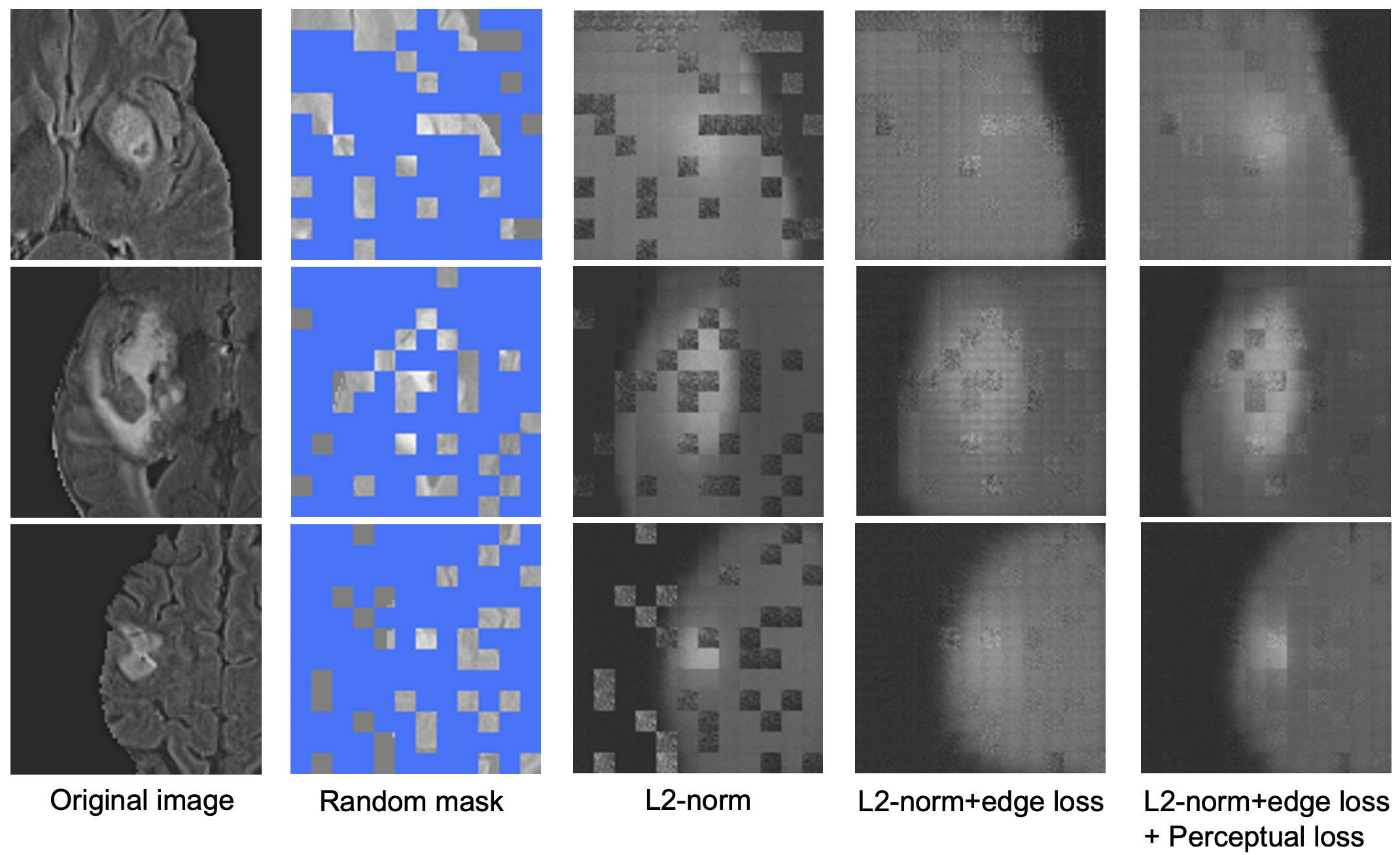
Figure 3: Effect of different loss functions for image reconstruction. We observe the progressive improvement of the reconstructed results from a fraction (25%) of the input.

We observe that ViT-AE$++$ behaves differently on two 3D datasets as shown in Table 3. On BraTS, ViT-AE$++$ is competitive to existing contrastive learning-based methods including MoCO-v3 Chen et al. (2021) and SimSiam Chen et al. (2020), achieving AUCs of 0.767 vs. 0.795 and 0.767 vs. 0.771 respectively. This may be caused by overfitting since BraTS has only 260 samples in each training fold. On EGD which contains two times amount of training samples, ViT-AE$++$ outperforms the two methods by a large margin, achieving AUCs of 0.846 vs. 0.734 and 0.846 vs. 0.741 respectively. Notably, the proposed new loss functions consistently improve the representation in the ViT-AE framework. As shown in Table 3, we observe that the auxiliary compound loss and contrastive loss improve vanilla ViT-AE significantly. Especially, to demonstrate the effectiveness of our proposed auxiliary compound loss, we visualize the reconstruction results by different combinations of reconstruction loss functions shown in Figure 3.

Table 2: Comparison of ViT-AE$++$ and other
self-supervised methods.

	BraTS	EGD
Methods	AUC	AUC
MoCO-v3	0.795 $\pm$ 0.065	0.734 $\pm$ 0.048
SimSiam	0.771 $\pm$ 0.065	0.741 $\pm$ 0.039
Vallina ViT-AE	0.696 $\pm$ 0.079	0.828 $\pm$ 0.036
ViT-AE++(ours)	0.767 $\pm$ 0.068	0.846 $\pm$ 0.034

Table 3: Ablation study of the auxiliary loss and contrastive loss on the BraTS dataset.

	BraTS
Methods	AUC
ViT$+\mathcal{L}_{CL}$	0.680 $\pm$ 0.091
ViT-AE	0.696 $\pm$ 0.057
ViT-AE+$\mathcal{L}_{edge}$	0.704 $\pm$ 0.065
ViT-AE+$\mathcal{L}_{Per}$	0.721 $\pm$ 0.085
ViT-AE+$\mathcal{L}_{edge}$+$\mathcal{L}_{Per}$	0.734 $\pm$ 0.088
ViT-AE+$\mathcal{L}_{edge}$+$\mathcal{L}_{Per}$+$\mathcal{L}_{CL}$	0.767 $\pm$ 0.069

Does backbone matter?

Our proposed framework used the vision transformer (ViT) as our feature extraction backbone. One might argue that the observed performance improvement is a consequence of using the ViT and not the proposed auxiliary training objectives. In such a scenario, plugging in the ViT in other self-supervised representation learning methods such as MoCOv3 He et al. (2020) and SimSiam Chen and He (2021) should lead to a corresponding increase in representation strength. Tab. 4 shows the results on the BraTs and EGD datasets. The self-supervised representation features learned using vision transformers perform poorly compared to their ResNet counterpart. We believe this results from overfitting due to a large number of model parameters in ViT. Thus, we conclude that a simple replacement of the feature extractor does not guarantee superior performance.

Table 4: Performances of vision transforms trained using different self-supervised representation learning methods.

	BraTS	EGD
Methods	AUC	AUC
MoCOv3	0.795 $\pm$ 0.057	0.734 $\pm$ 0.048
SimSiam	0.771 $\pm$ 0.065	0.741 $\pm$ 0.039
SimSiam (ViT)	0.605 $\pm$ 0.088	0.774 $\pm$ red0.033
MoCov3 (ViT)	0.714 $\pm$ 0.069	0.798 $\pm$ 0.029

Analysis of hyperparameters.

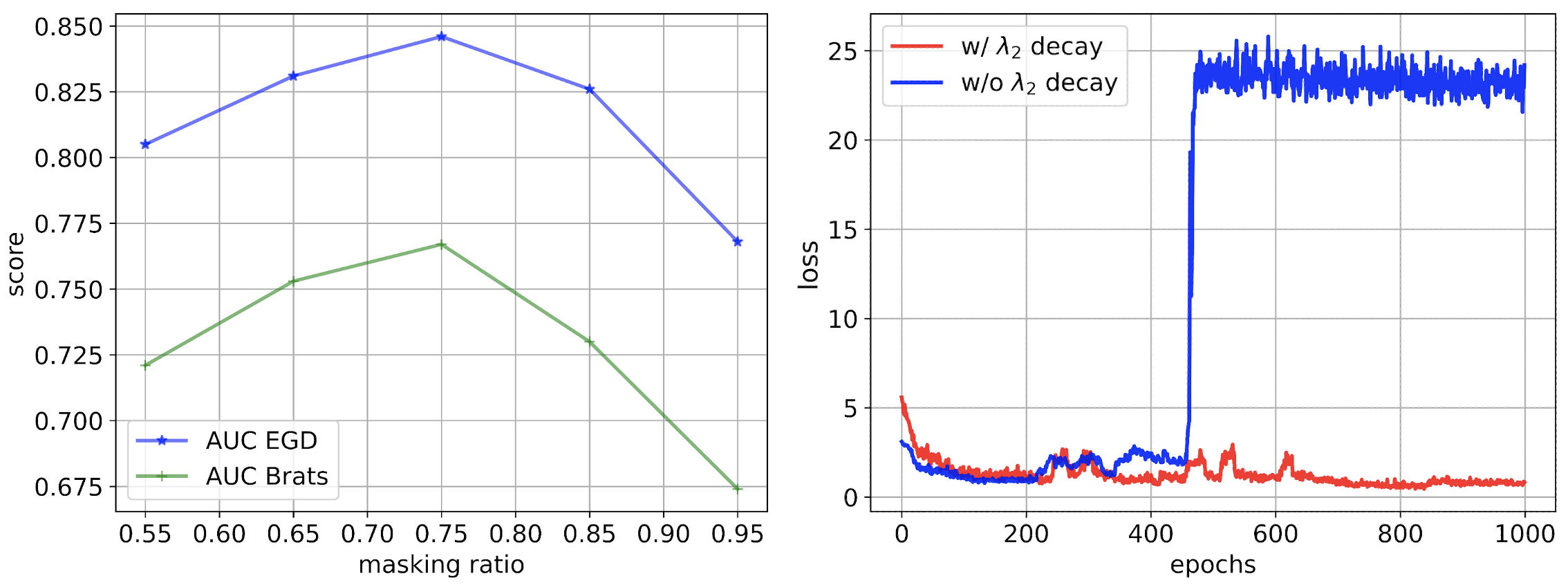
Figure 2: Effects of two key parameters. Left: Masking ratio vs. AUC on the BraTS dataset. The AUC and specificity increase with higher masking ratio, peaking at 0.75, after which they begin to decrease. Right: Training loss with Eq. 4 over epochs with and without weight decay of $\lambda_{2}$ for $\mathcal{L}_{edge}$. Without decay (blue), the loss may explode and the training could not converge; With decay (red), training is stable and converges.

We analyze two critical parameters in the proposed framework which affect the representation and training stability.

Effect of masking ratio $p$.

The masking ratio $p$ determines what percentage of the input volume is masked away. This, in turn, controls the difficulty of the reconstruction task. A higher value of $p$ implies fewer visible patches $X^{*}$, which makes reconstruction more challenging. On the other hand, a low $p$ can allow the model to extrapolate between visible patches, thus not learning good features. To find a suitable value of $p$, we run experiments with $p\in[0.55,0.65,0.75,0.85,0.95]$. The results for the BraTS dataset are summarized in Figure 2. We observe that the highest AUC value is obtained at $p=0.75$. In our experiments, the optimal value was $p=0.75$ for both datasets.

Weight decay for edge-based loss.

The edge-based loss weight $\lambda_{2}$ in Eq. 4 was decreased linearly with number of epochs. We observed that gradually decreasing $\lambda_{2}$ was essential for the training stability. One possible explanation for the instability is related to the one-to-multiple mapping of the reconstruction task. While the edge map $\mathcal{L}_{edge}$ provides strong additional supervision signals for reconstruction, it is sensitive to noise artifacts which can cause large losses. Fitting to such artifacts destabilizes the training process and hampers the embedding features. To avoid this overfitting, we start the training with $\lambda_{2}=0.01$ and linearly decrease it with each epoch. This allows the network to learn structural information initially and gradually focus more on perceptual similarity. The loss plot is shown in Fig.  2. Without a weight decay of $\lambda_{2}$, the loss tends to diverge. When using a linear decay, the training is stable and gradually converges.

6 Discussion and conclusion

We proposed ViT-AE$++$ to improve the existing vision transformer-based self-supervised learning approach, which is orthogonal to the existing contrastive learning-based approaches. We introduce a new auxiliary reconstruction loss to the vision transformer autoencoder and extend it with a contrastive loss. We demonstrate that our proposed method is superior to vanilla ViT-AE and competitive to contrastive learning-based methods We hope our work can provide a new perspective for representation learning in medical imaging and advance self-supervised features to the next level. In this work, we focus on learning representation on a single dataset and evaluate it in a downstream task using the same dataset. In future work, we will investigate learning generalizable self-supervised representations immune to common domain shifts (e.g., caused by image acquisition).

We would like to thank the Helmut Horten Foundation for supprting our research. Additionally, Hongwei Bran Li is supported by an Nvidia Academic GPU grant and Forschungskredit (grant No. K-74851-01-01) from the University of Zurich.

Appendix A

A.1 Reconstruction results

Table 5: Results of two qualitative metrics on image quality of reconstruction results generated by different methods in Fig. 5. The values are computed between the reference image and the reconstructed image.

	Sample 1	Sample 2	Sample 3
Methods	PSNR/SSIM	PSNR/SSIM	PSNR/SSIM
$\mathcal{L}_{2}$ norm	21.475/0.396	24.064/0.558	25.362/0.521
$\mathcal{L}_{2}$+$\mathcal{L}_{edge}$	24.497/0.503	26.751/0.565	26.891/0.571
$\mathcal{L}_{2}$+$\mathcal{L}_{edge}$+$\mathcal{L}_{per}$	25.339/0.514	27.211/0.572	27.703/0.586

A.2 3D Positional Encoding

In our setup, ViT deals with 96 $\times$ 96 $\times$ 96 cubes. The input volume is divided into patches of 8 $\times$ 8 $\times$ 8. A special CLS token is added to the input sequence (see Fig. 4). This token is used for downstream calculations. Fixed 3D sinusoidal encoding is used to inject positioning information to these patches, including the CLS token. There are 1729 input tokens (1728 patch tokens and one CLS token). Each axis encodes approximately $\frac{1}{3}$ of the input volume. The framework is flexible to work with different patch sizes.

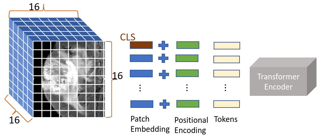
Figure 4: Position encoding representation. The given input volume is divided into a grid of size 16 $\times$ 16 $\times$ 16. A special CLS token is added along with the patch embeddings. 3D sinusoidal position encoding is added to each input patch (including the special CLS token). The position-aware tokens are fed into the Transformer encoder.

A.3 Perceptual loss and edge loss

For medical data, a pre-trained VGG-16 Simonyan and Zisserman (2015) is used to compute the perceptual similarity between the original volume and its reconstruction. The VGG network is pre-trained on 2D images and can not be directly used with 3D volumes. Hence, we compute loss along 2D slices of the input volume and its reconstruction. The per-slice loss values are averaged to obtain loss for the entire volume. The 3D $Sobel$ filter operation is shown in Fig. 5.

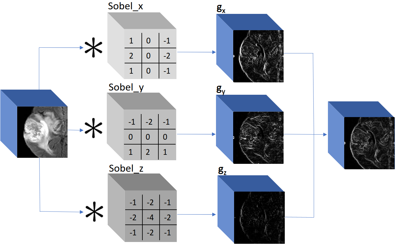
Figure 5: Schematic diagram of 3D Sobel filter. The 3D volume is convolved by 3 $\times$ 3 filters. The filter weights are fixed, and each filter computes the gradients in one specific direction. Sobel_x computes the gradients $g_{x}$ along the Sagittal plane (x-axis). Similarly, $g_{y}$ and $g_{z}$ are gradients along the Axial (y-axis) and Coronal (z-axis) planes, respectively. The final edge map is obtained by $\sqrt{g_{x}^{2}+g_{y}^{2}+g_{z}^{2}}$.

A.4 Sample X-ray images.

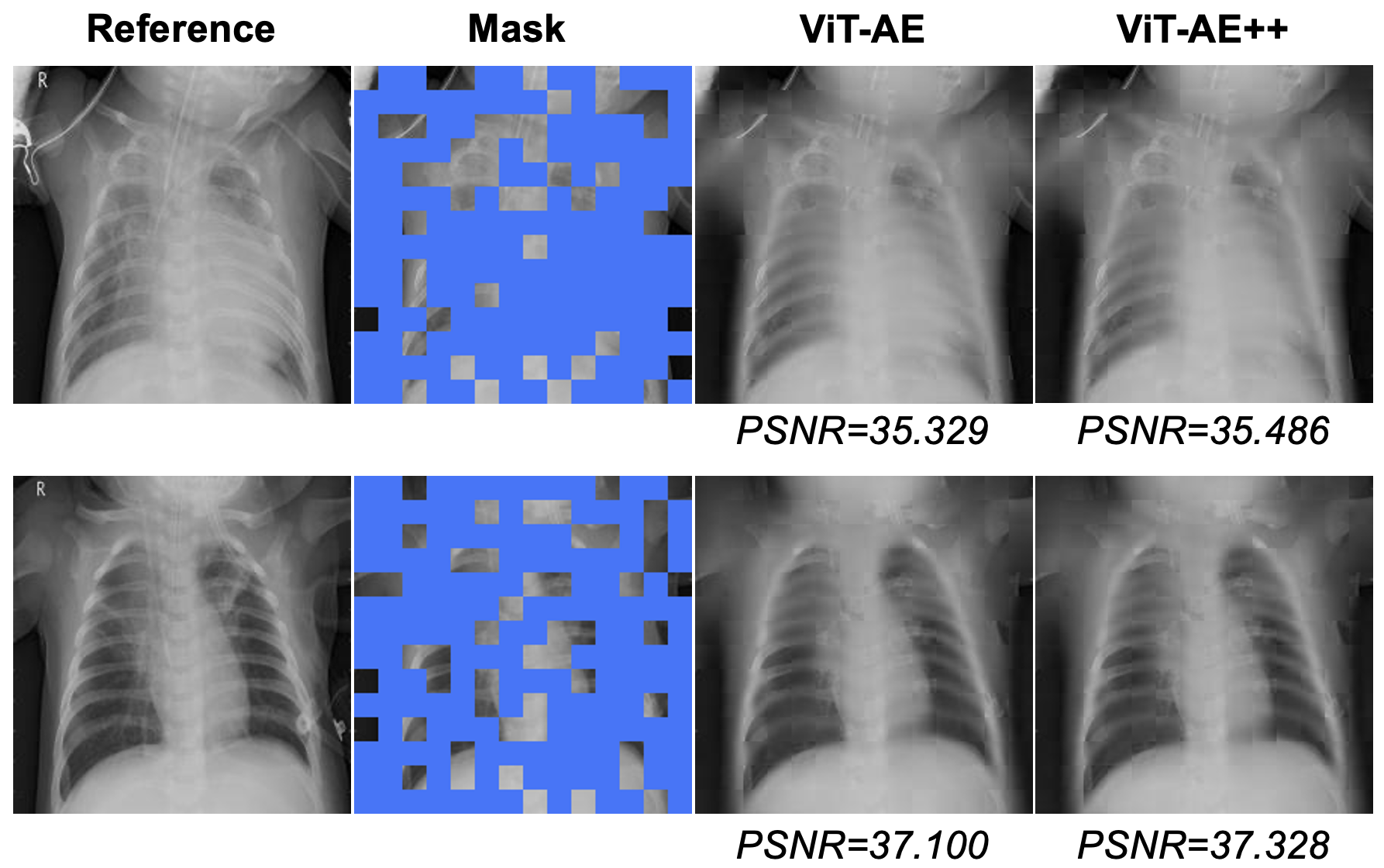
Figure 6: We observed that ViT-AE++ achieved significantly higher PSNR (p-value ¡ 0.0001) than ViT-AE. There is no statistical significance in SSIM.

References

- Bakas et al. (2018) Spyridon Bakas, Mauricio Reyes, Andras Jakab, Stefan Bauer, Markus Rempfler, Alessandro Crimi, Russell Takeshi Shinohara, Christoph Berger, Sung Min Ha, Martin Rozycki, et al. Identifying the best machine learning algorithms for brain tumor segmentation, progression assessment, and overall survival prediction in the brats challenge. arXiv preprint arXiv:1811.02629, 2018.
- Chaitanya et al. (2020) Krishna Chaitanya, Ertunc Erdil, Neerav Karani, and Ender Konukoglu. Contrastive learning of global and local features for medical image segmentation with limited annotations. arXiv preprint arXiv:2006.10511, 2020.
- Chen et al. (2020) Ting Chen, Simon Kornblith, Mohammad Norouzi, and Geoffrey Hinton. A simple framework for contrastive learning of visual representations. arXiv preprint arXiv:2002.05709, 2020.
- Chen and He (2020) Xinlei Chen and Kaiming He. Exploring simple siamese representation learning. arXiv preprint arXiv:2011.10566, 2020.
- Chen and He (2021) Xinlei Chen and Kaiming He. Exploring simple siamese representation learning. In Proceedings of the IEEE/CVF Conference on Computer Vision and Pattern Recognition, pages 15750–15758, 2021.
- Chen et al. (2021) Xinlei Chen, Saining Xie, and Kaiming He. An empirical study of training self-supervised vision transformers. In Proceedings of the IEEE/CVF International Conference on Computer Vision, pages 9640–9649, 2021.
- Devlin et al. (2019) Jacob Devlin, Ming-Wei Chang, Kenton Lee, and Kristina Toutanova. Bert: Pre-training of deep bidirectional transformers for language understanding, 2019.
- Dosovitskiy et al. (2021) Alexey Dosovitskiy, Lucas Beyer, Alexander Kolesnikov, Dirk Weissenborn, Xiaohua Zhai, Thomas Unterthiner, Mostafa Dehghani, Matthias Minderer, Georg Heigold, Sylvain Gelly, Jakob Uszkoreit, and Neil Houlsby. An image is worth 16x16 words: Transformers for image recognition at scale, 2021.
- Dufumier et al. (2021) Benoit Dufumier, Pietro Gori, Julie Victor, Antoine Grigis, Michele Wessa, Paolo Brambilla, Pauline Favre, Mircea Polosan, Colm Mcdonald, Camille Marie Piguet, et al. Contrastive learning with continuous proxy meta-data for 3d mri classification. In International Conference on Medical Image Computing and Computer-Assisted Intervention, pages 58–68. Springer, 2021.
- Goyal et al. (2018) Priya Goyal, Piotr Dollár, Ross Girshick, Pieter Noordhuis, Lukasz Wesolowski, Aapo Kyrola, Andrew Tulloch, Yangqing Jia, and Kaiming He. Accurate, large minibatch sgd: Training imagenet in 1 hour, 2018.
- Grill et al. (2020) Jean-Bastien Grill, Florian Strub, Florent Altché, Corentin Tallec, Pierre Richemond, Elena Buchatskaya, Carl Doersch, Bernardo Avila Pires, Zhaohan Guo, Mohammad Gheshlaghi Azar, et al. Bootstrap your own latent-a new approach to self-supervised learning. Advances in Neural Information Processing Systems, 33, 2020.
- He et al. (2020) Kaiming He, Haoqi Fan, Yuxin Wu, Saining Xie, and Ross Girshick. Momentum contrast for unsupervised visual representation learning. In Computer Vision and Pattern Recognition, pages 9729–9738, 2020.
- He et al. (2021) Kaiming He, Xinlei Chen, Saining Xie, Yanghao Li, Piotr Dollár, and Ross Girshick. Masked autoencoders are scalable vision learners. arXiv preprint arXiv:2111.06377, 2021.
- Johnson et al. (2016) Justin Johnson, Alexandre Alahi, and Li Fei-Fei. Perceptual losses for real-time style transfer and super-resolution. In European conference on computer vision, pages 694–711. Springer, 2016.
- Kanopoulos et al. (1988) Nick Kanopoulos, Nagesh Vasanthavada, and Robert L Baker. Design of an image edge detection filter using the sobel operator. IEEE Journal of solid-state circuits, 23(2):358–367, 1988.
- Kermany et al. (2018) Daniel S Kermany, Michael Goldbaum, Wenjia Cai, Carolina CS Valentim, Huiying Liang, Sally L Baxter, Alex McKeown, Ge Yang, Xiaokang Wu, Fangbing Yan, et al. Identifying medical diagnoses and treatable diseases by image-based deep learning. cell, 172(5):1122–1131, 2018.
- Lee et al. (2015) Chen-Yu Lee, Saining Xie, Patrick Gallagher, Zhengyou Zhang, and Zhuowen Tu. Deeply-supervised nets. In Artificial intelligence and statistics, pages 562–570. PMLR, 2015.
- Li et al. (2021) Hongwei Li, Fei-Fei Xue, Krishna Chaitanya, Shengda Luo, Ivan Ezhov, Benedikt Wiestler, Jianguo Zhang, and Bjoern Menze. Imbalance-aware self-supervised learning for 3d radiomic representations. In International Conference on Medical Image Computing and Computer-Assisted Intervention, pages 36–46. Springer, 2021.
- Liu et al. (2021) Yifan Liu, Hao Chen, Yu Chen, Wei Yin, and Chunhua Shen. Generic perceptual loss for modeling structured output dependencies. In Proceedings of the IEEE/CVF Conference on Computer Vision and Pattern Recognition, pages 5424–5432, 2021.
- Loshchilov and Hutter (2017) Ilya Loshchilov and Frank Hutter. Sgdr: Stochastic gradient descent with warm restarts, 2017.
- Loshchilov and Hutter (2019) Ilya Loshchilov and Frank Hutter. Decoupled weight decay regularization, 2019.
- Menze et al. (2014) Bjoern H Menze, Andras Jakab, Stefan Bauer, Jayashree Kalpathy-Cramer, Keyvan Farahani, Justin Kirby, Yuliya Burren, Nicole Porz, Johannes Slotboom, Roland Wiest, et al. The multimodal brain tumor image segmentation benchmark (BRATS). IEEE Transactions on Medical Imaging, 34(10):1993–2024, 2014.
- Oord et al. (2018) Aaron van den Oord, Yazhe Li, and Oriol Vinyals. Representation learning with contrastive predictive coding. arXiv preprint arXiv:1807.03748, 2018.
- Russakovsky et al. (2015) Olga Russakovsky, Jia Deng, Hao Su, Jonathan Krause, Sanjeev Satheesh, Sean Ma, Zhiheng Huang, Andrej Karpathy, Aditya Khosla, Michael Bernstein, et al. Imagenet large scale visual recognition challenge. International journal of computer vision, 115(3):211–252, 2015.
- Shen et al. (2017) Haocheng Shen, Ruixuan Wang, Jianguo Zhang, and Stephen J McKenna. Boundary-aware fully convolutional network for brain tumor segmentation. In International Conference on Medical Image Computing and Computer-Assisted Intervention, pages 433–441. Springer, 2017.
- Simonyan and Zisserman (2015) Karen Simonyan and Andrew Zisserman. Very deep convolutional networks for large-scale image recognition, 2015.
- van der Voort et al. (2021) Sebastian R van der Voort, Fatih Incekara, Maarten MJ Wijnenga, Georgios Kapsas, Renske Gahrmann, Joost W Schouten, Hendrikus J Dubbink, Arnaud JPE Vincent, Martin J van den Bent, Pim J French, et al. The erasmus glioma database (egd): Structural mri scans, who 2016 subtypes, and segmentations of 774 patients with glioma. Data in brief, 37:107191, 2021.
- Zeng et al. (2021) Dewen Zeng, Yawen Wu, Xinrong Hu, Xiaowei Xu, Haiyun Yuan, Meiping Huang, Jian Zhuang, Jingtong Hu, and Yiyu Shi. Positional contrastive learning for volumetric medical image segmentation. In International Conference on Medical Image Computing and Computer-Assisted Intervention, pages 221–230. Springer, 2021.
- Zhao et al. (2017) Hengshuang Zhao, Jianping Shi, Xiaojuan Qi, Xiaogang Wang, and Jiaya Jia. Pyramid scene parsing network. In Proceedings of the IEEE conference on computer vision and pattern recognition, pages 2881–2890, 2017.
- Zhou et al. (2019) Zongwei Zhou, Vatsal Sodha, Md Mahfuzur Rahman Siddiquee, Ruibin Feng, Nima Tajbakhsh, Michael B Gotway, and Jianming Liang. Models genesis: Generic autodidactic models for 3d medical image analysis. In Medical Image Computing and Computer-Assisted Intervention, pages 384–393, 2019.