New estimates of ongoing sea level change and land movements caused by Glacial Isostatic Adjustment in the Mediterranean region

Abstract

Glacial Isostatic Adjustment (GIA) caused by the melting of past ice sheets is still a major cause of sea-level variations and 3-D crustal deformation in the Mediterranean region. However, since the contribution of GIA cannot be separated from those of oceanic or tectonic origin, its role can be only assessed by numerical modelling, solving the gravitationally self-consistent Sea Level Equation. Nonetheless, uncertainties about the melting history of the late-Pleistocene ice sheets and the rheological profile of the Earth’s mantle affect the GIA predictions by an unknown amount. Estimating the GIA modelling uncertainties would be particularly important in the Mediterranean region, due to the amount of high quality geodetic data from space-borne and ground-based observations currently available, whose interpretation demands a suitable isostatic correction. Here we first review previous results about the effects of GIA in the Mediterranean Sea, enlightening the variability of all the fields affected by the persistent condition of isostatic disequilibrium. Then, for the first time in this region, we adopt an ensemble modelling approach to better constrain the present-day GIA contributions to sea-level rise and geodetic variations, and their uncertainty.

Key words: Sea Level Change – Mediterranean Sea – Glacial Isostatic Adjustment

This is a pre-copyedited, author-produced PDF of an article accepted for publication in Geophysical Journal International following peer review. The version of record [G. Spada, D. Melini, New estimates of ongoing sea level change and land movements caused by Glacial Isostatic Adjustment in the Mediterranean region, Geophysical Journal International, Volume 229, Issue 2, May 2022, Pages 984–998] is available online at: https://doi.org/10.1093/gji/ggab508

1 Introduction

Following the seminal works of Flemming (1978) and Pirazzoli (2005), the history of relative sea-level across the Mediterranean Sea during the last millennia has been the subject of a number of investigations. Often, these have been focused on specific areas from which paleo sea-level indicators are available, based upon geological, geomorphological and archaeological evidence during the last millennia (see Lambeck, 1995; Lambeck et al., 2004a, b; Sivan et al., 2001; Antonioli et al., 2009; Evelpidou et al., 2012; Mauz et al., 2015; Vacchi et al., 2016, 2018, and references therein). However, the reconstruction of the history of sea level since the Last Glacial Maximum is hampered by the complex geodynamic setting of the Mediterranean region (see Anzidei et al., 2014; Faccenna et al., 2014), where tectonics and isostasy are contributing simultaneously to vertical deformations and gravity variations, thus producing a complex pattern of relative sea-level change. With the aim of separating these effects, long-term relative sea-level data from the Mediterranean Sea have been often interpreted with the aid of global Glacial Isostatic Adjustment (GIA) models. These are based upon the Sea Level Equation (SLE) first introduced by Farrell & Clark (1976), which is solved adopting a specific deglaciation chronology for the late-Pleistocene ice sheets and an a priori rheological profile (Spada, 2017; Whitehouse, 2018).

Due to the delayed viscoelastic response of the Earth’s system to surface mass redistributions, signals from the last deglaciation are still detectable today across the Mediterranean region. Previous model computations of Stocchi & Spada (2007, 2009) have shown that these GIA imprints can significantly affect sea-level measurements at tide gauges, vertical and horizontal land motion observed by means of GNSS methods and absolute sea-level variations tracked by altimeters (Cazenave et al., 2002). Although the importance of the ongoing isostatic readjustment has been clearly recognized in a number of works (see e.g., Serpelloni et al., 2013; Anzidei et al., 2014), these contemporary regional effects of GIA have received comparatively little attention so far. Our new assessment, which builds upon previous work of Stocchi & Spada (2009), is motivated by the increasing number of high quality space-borne and ground-based geodetic data available across the Mediterranean region (Tsimplis et al., 2013; Bonaduce et al., 2016), the recent development of new global models of the ice history and the layered Earth structure parameters  (Peltier et al., 2015; Roy & Peltier, 2017) and the availability of new numerical tools (Spada & Melini, 2019a).

GIA models account for gravitational, deformational and rotational interactions within the Earth system and explain the spatial and temporal variability of sea level in response to surface mass redistributions (see Spada (2017) and Whitehouse (2018) for a review). In global studies, the fine details of the GIA imprint across the Mediterranean are scarcely appreciated, due to the relatively small extent of the basin (see e.g., Tamisiea, 2011). In this region, the ongoing sea-level variations due to GIA have been first visualized – but not discussed – in the work of Mitrovica & Milne (2002), who solved globally the SLE to a sufficiently high spatial resolution. Based upon a modified version of model ICE-3G (VM1) of Tushingham & Peltier (1991), the global maps of Mitrovica and Milne clearly show that GIA is still causing significant sea-level variations across the Mediterranean Sea. Maximum amplitudes of relative sea-level rise are reached in the bulk of the basin and decline toward the coastlines. The same peculiar pattern is predicted at adjacent mid-latitude basins, i.e., the Black Sea and the Caspian Sea. The GIA-induced relative sea-level rise originates from a basin-scale land subsidence, with the maximum rates attained in the bulk of the basin. These patterns of relative sea-level rise and land subsidence have been interpreted by Stocchi & Spada (2007) as an effect of the extra-loading exerted by meltwater on the seafloor during deglaciation (hydro-isostasy), which is still ongoing due to the persisting non-isostatic conditions. A role of the melting of the former Fennoscandian ice sheet has been invoked by Stocchi & Spada (2007), while the contribution from the deglaciation of the nearby Alpine ice sheet still remains uncertain (Stocchi et al., 2005; Sternai et al., 2019) despite the improvements in glaciological modelling (see Seguinot et al., 2018, and references therein).

The present regional imprint of GIA across the Mediterranean Sea has been studied in detail by Stocchi & Spada (2009), adopting some of the first ICE-$X$ models developed by WR Peltier and collaborators. They have considered predictions of a suite of GIA models in terms of rate of relative and absolute sea-level change and vertical land motion, both at a basin scale and at tide gauges locations, but paying no attention to possible horizontal motions. Since then, however, a number of improved GIA models consistent with global relative sea-level datasets has been introduced, including revised deglaciation chronologies and viscosity profiles, which until now have not been fully exploited to study the ongoing effects of GIA in the region (Peltier et al., 2015; Roy & Peltier, 2017). Furthermore, the former GIA simulations of Stocchi & Spada (2007, 2009) were obtained adopting a coarse spatial resolution, and some potentially important effects such as the rotational feedback on sea level and the horizontal migration of the shorelines were not considered. Of course, we should not expect that taking these features into account would profoundly affect our knowledge about the effects of GIA across the Mediterranean Sea. However, improving the modeling scheme by introducing an ensemble approach would certainly provide more robust results. Furthermore, upgraded GIA computations would facilitate the interpretation of geodetic data and provide up-to-date corrections to a number of observations. Last, the results of Melini & Spada (2019) suggest that an ensemble approach would be useful to constrain the uncertainties that are still involved in GIA modelling and to explore the future trends of sea level expected in the region. The importance of regional GIA modeling uncertainties has been also discussed by Love et al. (2016), Vestøl et al. (2019), Simon & Riva (2020) and Kierulf et al. (2021), although these works were not focused on the Mediterranean Sea.

The paper is organized as follows. The methods are briefly described in Section 2. In Section 3 we describe the imprints of GIA on several geophysical quantities in the Mediterranean region. Ensemble GIA modelling results are presented in Section 4 and discussed in Section 5. Our conclusions are drawn in Section 6.

2 Methods

All the GIA simulations in this work have been performed using the open source SLE solver SELEN⁴ (SELEN version 4, see Spada & Melini, 2019a), in which the published histories of deglaciation of the various GIA models and the rheological profiles of the mantle have been incorporated. However, in some instances, we have used GIA results directly available from the Datasets page of WR Peltier, which also provides details about the setup of the most recent models of the ICE-$X$ suite.

SELEN⁴ solves the gravitationally and topographically self-consistent SLE, which in its simplest form reads

$$S(\theta,\lambda,t)=N-U\,,$$ (1)

where $S(\theta,\lambda,t)$ is relative sea-level change at the location of colatitude $\theta$ and longitude $\lambda$, $t$ is time, while $N=N(\theta,\lambda,t)$ and $U=U(\theta,\lambda,t)$ are absolute sea-level change and the vertical displacement of the Earth’s surface, respectively. A thorough discussion of the physics of SLE is given in the seminal work of Farrell & Clark (1976) and in Tamisiea (2011).

Since both $N$ and $U$ implicitly depend on $S$, the SLE (1) is an integral equation that is solved numerically through an iterative scheme, which demands a suitable spatiotemporal discretization of the involved fields. We have defined a time discretization assuming constant steps of length $\Delta t=500$ years, over an integration interval that extends back to the Last Glacial Maximum. For the space discretization, we have taken advantage of the equal-area, icosahedron-based geodetic grid of Tegmark (1996), using a resolution parameter $R=100$ that corresponds to cells of size $\sim 20$ km on the surface of the Earth. The maximum degree of the analysis has been set to $l_{max}=512$, corresponding to a spatial wavelength of $\approx 75$ km. In some runs, to alleviate the computational burden, the parameters $R=60$ and $l_{max}=256$ have been adopted, without significant loss of precision in the final results. To prescribe the “final” (i.e., present-day) condition of Earth’s topography, we have adopted the bedrock version of the global ETOPO1 dataset (Amante & Eakins, 2009; Eakins & Sharman, 2012), integrated with the Bedmap2 topographic model (Fretwell et al., 2013) south of $60^{\circ}$S. The rotational feedback on sea-level change has been modeled according to the revised rotation theory of Mitrovica et al. (2005) and Mitrovica & Wahr (2011). The solution algorithm of the SLE consists of two nested iterations, where the external one updates the paleo-topography according to the solution of the SLE, which is performed in the internal iteration. In all the runs, we have adopted five external and five internal iterations to ensure convergence. Once $S$, $N$ and $U$ are obtained by solving iteratively the SLE (Eq. 1), a suite of additional geodetic quantities associated with GIA are accessible, as the East ($U_{e}$) and North ($U_{n}$) components of the horizontal displacement field and their present trends. For more details about the solution method, the reader is referred to the supplementary material of Spada & Melini (2019a).

3 GIA patterns in the Mediterranean region

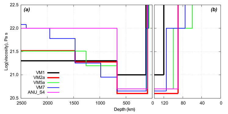
Figure 5: Radial viscosity profiles considered in this study. Frame (a) shows the full structure while (b) shows an enlarged view of the depth range $0$–$140$ km. VM1 assumes lower and upper mantle viscosities of $2\times 10^{21}$ Pa$\cdot$s and $10^{21}$ Pa$\cdot$s, respectively (Tushingham & Peltier, 1991). VM2a is a simplified version of the multi-layered VM2_L90 profile available from the web page of WR Peltier. Numerical values for VM5a and VM7 are from Table 2 of Roy & Peltier (2017). ANU_S4 assumes lower and upper mantle viscosities of $10^{22}$ and $5\times 10^{21}$ Pa$\cdot$s, respectively. Profiles VM5a and VM7 include a $40$ km-thick high-viscosity layer ($10^{22}$ Pa$\cdot$s) at the base of the lithosphere.

Figure 1 shows predictions for the ongoing rate of relative sea-level change across the Mediterranean Sea, hereafter denoted by ${\dot{S}}$, according to two state-of-the-art GIA models. The first model (Figure 1a), is the one progressively developed at the Australian National University (ANU) by Kurt Lambeck and collaborators (see e.g., Nakada & Lambeck, 1987; Lambeck et al., 2003). This map has been obtained by implementing the ANU ice chronology, provided to us by Anthony Purcell in November $2016$, into SELEN⁴; hence, this model shall be referred to as ANU$\_$S4 in the following. The setup of ANU$\_$S4 is based on a realization of the spatio-temporal evolution of ice complexes on a icosahedron-based global grid and assuming a piecewise constant time history, as described in Section 2 (see also Melini & Spada, 2019, for further details). The radial viscosity profile used in association with ANU_S4, shown in Figure 5, assumes a $90$ km elastic lithosphere and a viscosity of $5\times 10^{20}$ Pa$\cdot$s and $10^{22}$ Pa$\cdot$s in the upper and lower mantle, respectively (Lambeck et al., 2017).  The second model (Figure 1b) is ICE-6G$\_$C (VM5a), where “ICE-6G$\_$C” and “VM5a” denote its two basic components, namely the deglaciation chronology and the layered Earth structure parameters, respectively. This model, described by Argus et al. (2014) and Peltier et al. (2015) is one of the latest iterations of the suite of ICE-$X$ models historically developed at the University of Toronto by Prof. WR Peltier and collaborators.

The general patterns of sea-level change shown in Figure 1 confirm the results of Mitrovica & Milne (2002) and Stocchi & Spada (2009), clearly indicating that GIA is currently responsible for a general relative sea-level rise across the Mediterranean Sea. However, due to the high spatial resolution of these maps, the details of the non-uniform pattern of sea-level change caused by hydro-isostasy can be better discerned. The maximum values of ${\dot{S}}$, slightly exceeding the value of $0.4$ $\textrm{mm yr}^{-1}$, are attained across the widest sub-basins of the Mediterranean Sea, i.e., the Balearic, the Ionian, the Levantine and the Black seas. Stocchi & Spada (2007) have interpreted this pattern as the still progressing lithospheric flexure induced by the meltwater load, causing a sea-level rise relative to the seafloor, with maximum effects in the heart of the basins and its amplitude that declines approaching the shorelines. Of course, since the continental masses are unevenly distributed, the flexure due to subsidence shows a complex geometry, which is also partly determined by gravitational and rotational effects implicit in the SLE. It should be recalled that the two GIA models considered here are based upon different eustatic (i.e., ice-volume equivalent) curves, different deglaciation chronologies and rely upon distinct assumptions regarding the rheological profiles for the mantle. Despite these and other structural distinctions (for details, see Melini & Spada, 2019), in the Mediterranean region the $\dot{S}$ patterns are found to be broadly comparable. However, significant differences can be noted across the Levantine Sea and the Black Sea, where predictions based upon ICE-6G$\_$C (VM5a) generally exceed those obtained using ANU$\_$S4.

A noticeable feature of the GIA imprints in Figure 1 is the relatively small or even negligible value of ${\dot{S}}$ generally attained along the continental coastlines of Southern Europe and of North Africa, compared to the open sea. Interestingly, swathes of relative sea-level fall can be generally noted in places where the coastlines are characterized by a relatively short radius of curvature. For example, this is observed along the coasts of the Alboran Sea and of Tunisia, but also in the northern Aegean Sea and in the northern Adriatic Sea. In these marginal and narrow seas, the current trend of relative sea-level driven by GIA is dominated by the effect continental levering, which is manifested by subsidence of offshore locations and the upward tilting of onshore locations (see Walcott, 1972; Mitrovica & Peltier, 1991; Mitrovica & Milne, 2002; Murray-Wallace & Woodroffe, 2014; Clement et al., 2016). Condition ${\dot{S}}<0$ suggests that, at some time during the late Holocene, sea level may have been higher than today at these locations. Kearney (2001) has discussed about the possible existence of sea-level high-stands in the northern hemisphere during the Holocene and some works have reported evidence of high-stands, although without invoking isostatic mechanisms (see e.g., Pirazzoli et al., 1991; Bernier et al., 1993; Sanlaville et al., 1997; Morhange et al., 2006).  Remarkably, despite the structural differences, ICE-6G$\_$C (VM5a) and ANU$\_$S4 also broadly agree upon the position of possible Holocene high-stands, which are identified by the condition $\dot{S}<0$. In these locations, GIA is counteracting the general sea-level rise caused by the present-day terrestrial ice melt, which is characterized by very smooth imprints across the Mediterranean Sea (Galassi & Spada, 2014). Although tectonic deformations or factors associated to the ocean circulation could potentially overprint the isostatic contribution to sea level, evidence from specific sites like the Gulf of Gabès along the SE coast of Tunisia effectively confirms the existence of a late-Holocene high-stand (see e.g. Mauz et al., 2015). The existence of other possible high-stands along the coasts of the Mediterranean Sea, suggested by the map of Figure 1, shall be the topic of a follow-up study.

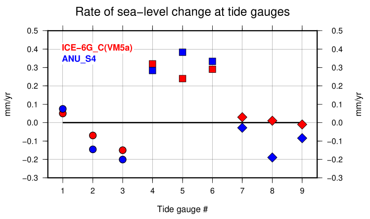
Figure 2: Rates of relative sea-level change $\dot{S}$ expected at tide gauges according to models ICE-6G$\_$C (VM5a) (red) and ANU$\_$S4 (blue). The tide gauges locations are marked by green symbols in Figure 1, which also shows the station names abbreviations. Numerical values of the rates are listed in Table 2.

A more quantitative  inter-comparison  between the  predictions  of models  ICE-6G$\_$C (VM5a)  and ANU$\_$S4 is drawn in Figure 2, showing the values of ${\dot{S}}$ at specific locations where several tide gauges are sited (see green symbols in Figure 1). The sites of Marseilles (1), Genova (2) and Trieste (3), marked by circles, have a particular importance since they are all characterized by long records and therefore they have been considered in various estimates of secular global mean sea-level rise (see e.g., Douglas, 1991; Woodworth, 2003; Douglas, 1997; Spada & Galassi, 2012). Despite the short distance separating the sites (see Figure 1), the contribution of GIA to ${\dot{S}}$ is not uniform at these locations. However, it has a relatively modest amplitude, varying in the range between $\sim-0.2$ and $\sim+0.1$ $\textrm{mm yr}^{-1}$, according to both GIA models. In the western (Alicante I, 7) and in the eastern Mediterranean, at Hadera (8) and Alexandria (9) (diamonds), a similar range of responses is found for ANU$\_$S4 while ICE-6G$\_$C (VM5a) points to negligible values. It is apparent that consistent with the pattern of Figure 1, significant values of ${\dot{S}}$ are only expected at tide gauges located in the bulk of the basin. Indeed, at the sites of Palma de Mallorca (4), Cagliari (5) and Valletta (6) (squares), rates as large as ${\dot{S}}\sim 0.4$ $\textrm{mm yr}^{-1}$ are predicted by both models. For Cagliari, this is a significant fraction of the long-term rate of sea-level rise effectively observed in situ ($1.88\pm 0.24$ $\textrm{mm yr}^{-1}$), where we note that the GIA effect exceeds the standard error of the trend. A similar rate ($1.57\pm 1.12$ $\textrm{mm yr}^{-1}$) is observed at Valletta (or Marsaxlokk), although the GIA contribution is smaller than the uncertainty. For Mallorca, the time span of the data ($1997$-$2018$) is too short to establish a reliable trend. For reference, the numerical values of the ${\dot{S}}$ values portrayed in Figure 2 are reported in Table 2 below, along with the values obtained by the ensemble modelling approach described in Section 4.

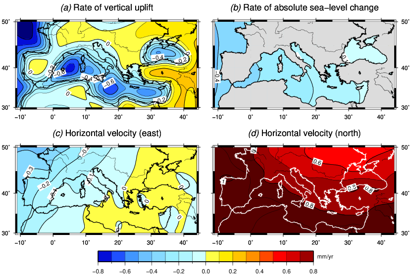
Figure 3: Predictions for the rate of vertical displacement ($\dot{U}$, a), of absolute sea-level change ($\dot{N}$, b), of the east component of horizontal displacement ($\dot{U}_{e}$, c) and for the north component ($\dot{U}_{n}$, d). All the maps are based upon model ICE-6G$\_$C (VM5a). Data are from the Datasets page of WR Peltier.

To better characterize the ongoing geodetic variations in the Mediterranean Sea, in Figure 3 we now consider a further set of variables associated with GIA, in addition to ${\dot{S}}$. These are the rate of vertical uplift ($\dot{U}$), the rate of absolute sea-level change ($\dot{N}$), as well as the East ($\dot{U}_{e}$) and North ($\dot{U}_{n}$) components of the horizontal rate of displacement. The latter components were not considered in Stocchi & Spada (2009) nor in subsequent works regarding the Mediterranean region. We note that ${\dot{S}}$, ${\dot{N}}$ and ${\dot{U}}$ are not independent of one another, being connected through the Sea Level Equation (1). The complexity of the four patterns in Figure 3, all pertaining to model ICE-6G$\_$C (VM5a), is apparent, and confirms that GIA has an important role in the spatial variability of present-day geodetic signals across the Mediterranean Sea. Similar results, not shown here, are obtained for model ANU$\_$S4. It is apparent that $\dot{U}$ (Figure 3a) is strongly anti-correlated with $\dot{S}$ (see Figure 1a), showing a widespread (but not uniform) state of subsidence across the whole Mediterranean basin, with maximum values of $-0.6$ $\textrm{mm yr}^{-1}$. We note that with the exception of some very narrow inlets, GIA is causing a general subsidence of all the coastlines ($\dot{U}<0$), including those stretches where $\dot{S}<0$, i.e., where a Holocene high-stand is expected (see Figure 1a). The pattern of $\dot{N}$ (b) shows that absolute sea level is falling across the whole Mediterranean basin, opposite to relative sea-level change $\dot{S}$. Furthermore, in contrast with $\dot{U}$, the rate of absolute sea-level change $\dot{N}$ shows little spatial variability and attains relatively small values with respect to $\dot{U}$. These are comparable with the global ocean-average $<\dot{N}>~{}\approx~{}-0.3$ $\textrm{mm yr}^{-1}$ (Melini & Spada, 2019; Spada & Melini, 2019b), which constitutes the GIA correction to absolute sea-level variations detected by satellite altimetry (see e.g., Tamisiea, 2011). According to the patterns in Figures 3c and 3d, the rates of horizontal displacements have a significant amplitude. In particular, the neatly positive $\dot{U}_{n}$ values (d) indicate that GIA is currently imposing a nearly uniform northward drift across the whole Mediterranean region, at a rate of $\sim~{}0.8$ $\textrm{mm yr}^{-1}$. By a global analysis, we have confirmed that this geodetically significant drift, whose amplitude remarkably exceeds $\dot{U}$ and $\dot{S}$, is to be attributed to the effect of the melting of the Laurentian and northern Europe ice sheets. The east component $\dot{U}_{e}$ has a minor role, with an amplitude not exceeding $\sim 0.1$ $\textrm{mm yr}^{-1}$ across the Mediterranean Sea (c). The GIA-induced northward drift notably exceeds the vertical rates. However, it is not expected to affect significantly the velocity fields observed by GNSS networks, which are dominated by larger tectonic signals (see, e.g. Faccenna et al., 2014).

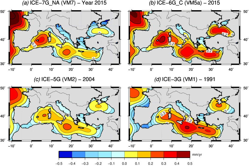
Figure 4: Rates of present day relative sea-level change $\dot{S}$ in the Mediterranean region, according to some combinations of ice deglaciation histories and viscosity profiles belonging to the ICE-$X$ suite of WR Peltier and collaborators. The model name and the date of publication are given in the headers. All the computations have been performed using program SELEN⁴.

Since GIA models are continuously evolving, their predictions are not given once and for all (Melini & Spada, 2019). To get a flavor of how the evolution of GIA models has influenced the pattern of ${\dot{S}}$ across the Mediterranean region, in Figure 4 we consider results for some members of the suite of ICE-$X$ models historically developed by WR Peltier and collaborators. They include model ICE-7G$\_$NA (VM7) of Roy & Peltier (2015) and its precursors ICE-6G$\_$C (VM5a) (Peltier et al., 2015), ICE-5G (VM2) (Peltier, 2004) and ICE-3G (VM1) (Tushingham & Peltier, 1991, 1992). For results based upon the first model of the suite (i.e., ICE-$1$ of Peltier & Andrews 1976), see Stocchi & Spada (2009). These GIA models have been introduced to progressively improve the fit with global sets of Holocene sea-level proxies and geodetic data. They are characterized by distinct rheological profiles and different melting histories of the continental ice sheets (see the references quoted above for details). All the runs in Figure 4 have been performed using the open source program SELEN⁴ (Spada & Melini, 2019a), in which the published histories of deglaciation and the rheological profiles of the mantle, shown in Figure 5, have been assimilated. We remark that differences between the SELEN⁴ results and those published in the original works are possible, as it can be seen comparing Figure 4b with Figure 1a, both pertaining to ICE-6G$\_$C (VM5a). These may reflect differences in the numerical schemes adopted to solve the SLE, in the theory employed to describe the rotational feedback on sea-level change, in the geometry and resolution of the grid on which the SLE is discretized, and in the nature of mantle layering (see Melini & Spada, 2019). These differences shall be understood as soon as a suite of benchmark computations will be established among SLE solvers, along the lines of previous efforts within the GIA community (Spada et al., 2011; Martinec et al., 2018; Kachuck & Cathles, 2019). From Figure 4 it is apparent that all the ICE-$X$ models broadly agree on the ${\dot{S}}$ patterns, which are all characterized by a sea-level rise in the bulk of the basin, also suggesting possible Holocene high-stands in the narrower inlets. However, it is clear that the patterns vary significantly in the details and that peak values attained in the various sub-basins of the Mediterranean Sea also differ. Overall, the variance of the results in Figure 4 clearly indicates that GIA predictions are affected by a significant degree of uncertainty on the Mediterranean scale. This justifies an ensemble approach involving a larger population of state-of-the-art GIA models.

4 Ensemble GIA modelling in the Mediterranean region

During the last decade, the importance of evaluating the uncertainties associated with GIA modelling has been recognized in a number of studies, and assessed through ensemble-like approaches. Until now, this has been done in various regional and global contexts, but never in the Mediterranean Sea. For example, in a re-analysis of Gravity Recovery and Climate Experiment (GRACE) measurements, Sasgen et al. (2012) have inverted the mass balance of the Antarctic ice sheet during 2002–2011 solving the forward GIA problem for a very rich set of models. Subsequently, using Bayesian methods and testing a large amount of GIA models, Caron et al. (2018) have evaluated uncertainties associated with imperfect knowledge of mantle viscosity upon the Stokes coefficients of the Earth’s gravity field. Uncertainties in 1-D GIA modelling have also been evaluated in an ensemble modelling perspective by Melini & Spada (2019), with the purpose of assessing their influence upon estimates of secular sea-level rise. Shortly after, Li et al. (2020) considered GIA uncertainties in the regional context of North America, accounting for the possible effects of 3-D Earth’s structure. Using an ensemble approach, Sun & Riva (2020) have built a global semi-empirical GIA model based on GRACE data. Melini & Spada (2019) and Li et al. (2020) have classified the GIA modelling uncertainties into two types. The first type (T1) is associated with the input parameters of the GIA models, e.g., the Earth viscosity profile or the loading history of continental ice sheets. The second type (T2) is associated with structural differences among GIA models. These include, for example, different numerical approaches to the solution of the SLE, the use of different eustatic curves, the adoption of different sets of geophysical constraints, or diverging a priori assumptions about the Earth’s viscosity profile. Possible ambiguities in the proposed classification of GIA modelling uncertainties however exist, as discussed by Melini & Spada (2019).

Characterizing GIA uncertainties at the Mediterranean scale is a challenging task. Indeed, a major issue arises because of the imperfect knowledge about regional-scale rheological heterogeneities, which certainly exist in such a complex tectonic setting (see Faccenna et al., 2014, and references therein). This would motivate, in the study area, a fully 3-D GIA modelling approach, which is however far from being realized. Limiting our attention to 1-D GIA modelling, here we take inspiration from previous multi-modelling approaches by Lambeck & Purcell (2005) and Roy & Peltier (2015), who have considered GIA modelling uncertainties into two different contexts. The study of Lambeck & Purcell (2005) is of particular relevance here, since it investigates the sensitivity of Holocene sea level at some Mediterranean sites to variations of the GIA model parameters. Lambeck & Purcell found that, at specific locations along the Mediterranean coastlines, relative sea-level predictions based on distinct rheological profiles can vary up to a few meters between $12$ and $6$ ka. However, their work was not dedicated to the evaluation to the GIA contribution to sea-level trends at present time, which is the target of our analysis. More recently, Roy & Peltier (2015) computed synthetic relative sea-level curves at selected North American sites using a suite of variants of the VM5a viscosity profile. They found that the thickness of the lithosphere and the viscosity structure of the upper mantle have an important influence on the relative sea level predictions, while the viscosity at depth significantly affects the spatiotemporal evolution of the lateral fore-bulge. It is of interest here to test whether these variants of the VM5a rheological profile can also influence the present-day sea-level change predictions in the Mediterranean region, away from the former centers of deglaciation.

To model the GIA contribution to sea-level rise in the Mediterranean region and its uncertainty, we have built two independent ensembles based upon previous works of Lambeck & Purcell (2005) and Roy & Peltier (2015), respectively. Since these works have been carried out independently and have proposed structurally distinct GIA models, based on different datasets, merging them in a unique ensemble would not be appropriate. Results obtained from the two ensembles should not be expected to overlap and could show a different sensitivity to the parameters that define each of the models. The first ensemble (E1) encompasses different realizations of model ANU$\_$S4, all sharing the same deglaciation chronology. Following Lambeck & Purcell (2005), the thickness of the elastic lithosphere and the upper and lower mantle viscosities are varied within the ranges listed in Table 1. Coherently with Lambeck & Purcell (2005), in building ensemble E1 we assume a nominal model with an upper mantle viscosity of $3\times 10^{20}$ Pa$\cdot$s and a lithospheric thickness of $65$ km. These values differ from those that we have used in ANU_S4, which is based on the rheological profile used for global-scale GIA models by the ANU group (see e.g. Lambeck et al., 2017). We shall therefore refer to this variant of of ANU_S4 as ANU_S4(E1). Ensemble E1 consists of $42$ GIA models. The second ensemble (E2), which consists of $74$ models, is originated from ICE-6G$\_$C (VM5a), considering variations of the lithospheric thickness and of the viscosity of each of the four mantle layers that characterize VM5a. The range of variability of each parameter is chosen to encompass the discrete values explored by Roy & Peltier (2015) (see Table 1), keeping the deglaciation chronology of ICE-6G$\_$C unaltered. In both ensembles, we vary a single rheological parameter within a pre-assigned range while keeping all the others fixed to their nominal value. When the lithospheric thickness is varied, we keep its elastic constants fixed to the PREM (Preliminary Reference Earth Model, see Dziewonski & Anderson 1981) averages obtained for the nominal model and, for ensemble E2, we retain a $40$ km-thick, high-viscosity layer at the base of the lithosphere (see Figure 5).

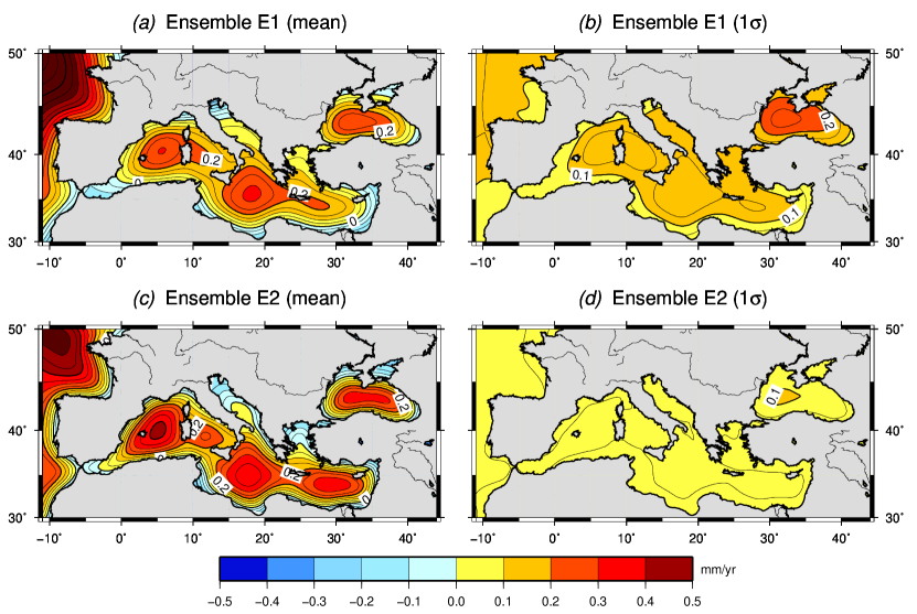
Figure 6: Averages (left) and standard deviations (right) obtained from the GIA ensembles E1 (based upon ANU_S4(E1)) and E2 (based upon ICE-6G$\_$C (VM5a)) for the present-day rate of sea-level change across the Mediterranean region. Standard deviations are relative to the average models shown in the left frames.

In Figure 6 the average $\dot{S}_{avg}$ and the standard deviation $\sigma_{\dot{S}}$ of E1 and E2 are shown, for the current rate of relative sea-level change. At a given location of coordinates $(\theta,\lambda)$, the standard deviation is $\sigma_{\dot{S}}=\sqrt{\sum_{i=1}^{n}(\dot{S}_{i}-\dot{S}_{avg})^{2}/(n-1)}$, where $n$ is the number of samples in the ensemble. The general patterns are broadly comparable, and both maps still confirm the existence of late-Holocene high-stands and substantially agree on their former position. However, some significant qualitative differences can be evidenced: i) sub-basin peak values for E2 generally exceed those based upon E1, ii) the E2 map is characterized by steeper gradients compared to E1, especially near the coastlines, iii) the uncertainty (1-$\sigma$) associated to E1 exceeds that of E2.

To gain a better insight into the different patterns obtained in Figure 6, in Figures 7 and 8 we consider in detail the sensitivity of $\dot{S}$ to individual rheological parameters. More specifically, each of the panels show the standard deviations of the $\dot{S}$ map obtained by varying each parameter within the range listed in Table 1. The standard deviations are relative to the prediction ${\dot{S}}_{nom}$ obtained for the nominal model, which is defined by the values given in parentheses in Table 1. At a given position, the standard deviations have been computed by $\sigma_{\dot{S}}=\sqrt{\sum_{i=1}^{n}({\dot{S}}_{i}-{\dot{S}}_{nom})^{2}/n}$, where $n$ is the number of models in the sub-ensemble corresponding to variations of the chosen parameter. For the ensemble E1, sensitivity to the lithospheric thickness (Figure 7a) reaches a peak level of $0.1$ $\textrm{mm yr}^{-1}$ at the center of the Ionian, Balearic and Black seas, while it is generally minimum near the shorelines. This pattern, which is correlated to the regional imprint of $\dot{S}$ (see Figure 1), hints to the role of lithospheric flexure due to the meltwater load. Sensitivity to the upper mantle viscosity (Figure 7b) is found to be considerably enhanced, with peak standard deviations in the range between $0.2$ and $0.4$ $\textrm{mm yr}^{-1}$ in the central regions of the sub-basins. As for the lithospheric thickness, the lowest sensitivity is generally found across the coastlines, with the notable exception of the Adriatic and Black seas. The sensitivity to the lower mantle viscosity (Figure 7c) shows a completely different regional imprint, with standard deviations increasing from the North African coast towards the northern margin of the basin. This pattern suggests an effect of the viscosity at depth on the shape of the fore-bulge of the northern Europe ice sheets, as pointed out by Roy & Peltier (2015) for the North American ice complex.

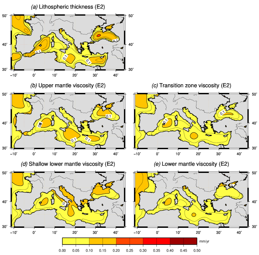
Figure 8: Standard deviation of $\dot{S}$, evaluated varying individual rheological parameters, for the ensemble E2, constructed using model ICE-6G$\_$C (VM5a). Standard deviations are relative to the nominal model ICE-6G$\_$C (VM5a).  

Figure 8 shows the sensitivity to the rheology of present-day $\dot{S}$ predicted by the ICE-6G (VM5a) GIA model, obtained through the analysis of the E2 ensemble. Here, in addition to the thickness of the elastic lithosphere, the viscosities of each of the four layers assumed by the VM5a model have been independently explored. For each parameter, the pattern of the standard deviations appears correlated to the spatial variability of $\dot{S}$ (see Figure 1), with peak values found in the central areas of the sub-basins. The sensitivity to lithospheric thickness (Figure 8a) turns out to be higher than in ANU$\_$S4, with standard deviations of $0.2$ $\textrm{mm yr}^{-1}$ found in the Balearic, Levantine and Black seas. Conversely, the sensitivity to the upper mantle viscosity structure (b and c) is much smaller than in ANU$\_$S4, with standard deviations values not exceeding the $0.1$ $\textrm{mm yr}^{-1}$ level both for the upper mantle and the transition zone viscosities. A similar pattern is found for the sensitivity to the lower mantle viscosity (d), while for the viscosity of the shallow part of the lower mantle (e) the general imprint correlated with $\dot{S}$ is superimposed to a northward-increasing gradient, with peak values of $0.2$ $\textrm{mm yr}^{-1}$ in the northern Adriatic and across the Crimean Peninsula. We note that, while the range of variability for the lithospheric thickness and lower mantle viscosity are considerably different between the two ensembles, all other viscosities are varied within comparable ranges of $0.7$–$0.8$ log Pa$\cdot$s. The reduced sensitivity to the upper mantle viscosity profile shown by ICE-6G may be related to the smaller viscosity contrasts assumed by VM5a with respect to ANU$\_$S4; on the other hand, the pattern of the standard deviations for the shallow lower mantle viscosity hints, as for ANU$\_$S4, to the imprint of the lateral fore-bulge of the northern European ice complexes.

5 Discussion

Previous work has clearly indicated that a correct interpretation of a number of geodetic signals, either regional or global, requires the proper evaluation of uncertainties associated with GIA modelling (King et al., 2010; Sasgen et al., 2012; Caron et al., 2018; Melini & Spada, 2019; Li et al., 2020). For the first time, in this work we have explored in detail the features of various GIA signals across the Mediterranean Sea, creating ensembles based upon up-to-date models recently proposed in the literature. Our study has been essentially motivated by the considerable amount of data indicating the variability of sea level in the past (Sivan et al., 2001; Antonioli et al., 2009; Lambeck & Purcell, 2005; Vacchi et al., 2016) and the by efforts made to constrain the current deformations and sea-level variability by high-quality geodetic observations (Fenoglio-Marc, 2002; Serpelloni et al., 2013; Bonaduce et al., 2016). Furthermore, the quality of existing data calls for a thorough evaluation of GIA modelling, improving upon previous works in which now outdated GIA models have been used or some physical ingredients of the SLE have been not taken into account (see e.g., Stocchi & Spada, 2009). Assuming a spherically symmetric Earth structure with a linear viscoelastic rheology, two ensembles of GIA models have been proposed, starting from structurally different nominal models developed by the two independent schools led by Kurt Lambeck (Australian National University) and WR Peltier (Univ. of Toronto), respectively. Overall, the two ensembles encompass $\sim 120$ GIA models, a small number compared to the GIA ensemble of Caron et al. (2018) but largely improving the “mini-ensemble” approach of Melini & Spada (2019). The range of viscosity profiles that we have adopted has been suggested by previous works by the two groups (see Lambeck & Purcell 2005 and Roy & Peltier 2015, respectively). Although limited to $1$-D Earth’s structures, our results clearly suggest that a high-resolution approach is necessary in order to capture the small-scale details of the ongoing GIA contributions across the study region, which are characterized by a striking regional variability despite the relatively narrow region. This variability is particularly enhanced for the fields $\dot{S}$ and $\dot{U}$, while $\dot{N}$, $\dot{U}_{n}$ and $\dot{U}_{e}$ are characterized by a comparatively smoother pattern although some of them have a significant amplitude.

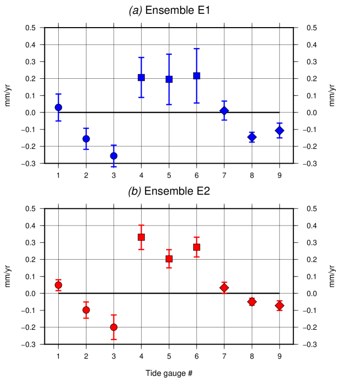
Figure 9: Ensemble average predictions of $\dot{S}$ at Mediterranean tide gauges and their $1$-$\sigma$ uncertainties, according to ensemble E1 (top) and E2 (bottom). The locations of the tide gauges are shown in Figure 1. Standard deviations are relative to the ensemble average. Numerical values are listed in Table 2.

In previous investigations aimed at studying the sea-level variability in the Mediterranean Sea (see e.g. Bonaduce et al., 2016) the effects of GIA have been estimated using a single model and focussing on the tide gauge locations, without considering the pattern of the GIA imprint across the whole region and neglecting the possible uncertainties involved in modelling. In other studies (see e.g. Santamaría-Gómez et al., 2017) the uncertainty has been roughly estimated by considering the predictions by two independently developed GIA models, basically adopting the “mini-ensemble” approach followed by Melini & Spada (2019). In Figure 9 we consider the same nine tide gauges whose locations are marked by green symbols in Figure 1. For each of them we show the average GIA contribution to the rate of relative sea-level change and its $1$-$\sigma$ uncertainty estimated by the two ensembles E1 (top) and E2 (bottom) introduced in previous section. For ensemble E1, it clearly appears that tide gauge sites located in islands in the bulk of the Mediterranean basin (sites $4$, $5$ and $6$) are characterized by the larger GIA rates, but also by the largest uncertainties. Conversely, in places located along the continental coastlines the GIA rates are comparatively modest, and generally less uncertain. This trade-off is less evident when we consider the ensemble E2, which is generally characterized by smaller uncertainties compared with E1. The results of Figure 9, along with the patterns shown in Figure 6, clearly indicate that the $\dot{S}$ values expected at tide gauges fall on the range between $-0.3$ and $0.5$ $\textrm{mm yr}^{-1}$, values that are smaller than those predicted in formerly de-glaciated areas by one order of magnitude (see e.g., Melini & Spada, 2019), regardless of the ensemble considered. Although the $1$-$\sigma$ uncertainties show a significant regional variability across the Mediterranean basin, our results suggest that they may attain a maximum value of $0.2$ $\textrm{mm yr}^{-1}$.

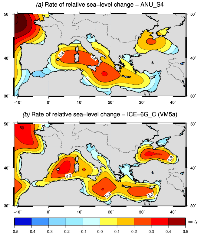
Figure 10: GIA rates of relative sea-level change ($\dot{S}$) expected in two thousands years across the Mediterranean Sea, according to the two models ANU$\_$S4 (a) and ICE-6G$\_$C (VM5a) (b).

Up to now, our attention has been limited to the ongoing geodetic variations due to GIA. In GIA modelling, these variations are generally assumed to be constant on a century time scale, since it is expected that the relatively high average mantle viscosity would prevent a significant decay (see e.g., Galassi & Spada, 2014; Spada & Galassi, 2015). To test this hypothesis, in Figure 10 we have projected the $\dot{S}$ GIA imprints over the next two millennia, using the two models ANU$\_$S4 and ICE-6G$\_$C (VM5a) whose contemporary imprints have been considered already in Figure 1. It is useful to remark that according to these two models (see Table 1), the bulk viscosity of the mantle is not too dissimilar from the “Haskell value” of $10^{21}$ Pa $\cdot$ s (see Mitrovica, 1996, and references therein), so that a relaxation time of a few millennia would be expected (see e.g. Turcotte & Schubert, 2014). Indeed, the two figures show that the GIA rates are expected to decrease considerably (by $\sim 50\%$) over the next two millennia, leaving the general pattern of $\dot{S}$ basically unmodified with respect to the current imprint. At the same time, we have verified that the rates would be effectively unchanged over one century across the whole Mediterranean Basin. We note, however, that the nearshore mitigating effect of GIA ($\dot{S}<0$) will yet persist at some specific locations, although it is not expected that these relatively small rates (a few fractions of millimeters per year) would significantly counteract the general rising trend of sea-level due to climate change over next millennia (see e.g., Slangen et al., 2012).

6 Conclusion

In this work, we have obtained a set of high-resolution numerical solutions for the SLE at the Mediterranean scale, based on two up-to-date GIA models independently developed by the research groups led by Kurt Lambeck and WR Peltier. We have shown that some spatial features of the $\dot{S}$ maps are remarkably common between the two GIA models: i): peak values of $\dot{S}$, of about $0.4$ $\textrm{mm yr}^{-1}$, are attained in the central sub-basins, hinting to the effect of lithospheric flexure in reponse to hydrostatic load; ii) swaths of sea-level fall ($\dot{S}<0$) are present in narrow coastal inlets, implying the possible existence of Holocene high-stands, suggested by some works in the literature.  Rates of horizontal displacements due to ongoing isostatic readjustment point to a nearly uniform northward drift across the Mediterranean, associated with the collapse of the northern European ice sheet fore-bulges. With an amplitude of $\sim 0.8$ $\textrm{mm yr}^{-1}$, this northward drift notably exceeds the vertical rates.

Through an ensemble approach, we assessed the model uncertainties associated to present-day GIA across the Mediterranean basin. Uncertainties on $\dot{S}$ are generally correlated with the amplitude of the field and reach the $0.1$ $\textrm{mm yr}^{-1}$ level in the central sub-basins. A remarkable exception is seen for the ensemble based on ANU$\_$S4, for which a sensitivity to the viscosity structure in the upper mantle reaches the $0.4$ $\textrm{mm yr}^{-1}$ level, possibly associated to the enhanced viscosity contrasts assumed by ANU$\_$S4 and to the correspondingly weaker upper mantle viscosities explored in ensemble E1. In both ensembles, the spatial pattern of sensitivity to the lower mantle viscosity presents a north-south trending gradient, hinting to a long-wavelength effect associated with the isostatic response to the melting of Fennoscandian ice complexes. For a more comprehensive assessment of the GIA modeling uncertainties in the Mediterranean Sea, the regional-scale geodynamical setting would need to be taken into consideration. However, the structural complexity of region can only be accounted for through a 3-D numerical approach, which is far beyond the reach of the class of GIA models considered in this study.

Data availability

The data underlying this article will be shared on reasonable request to the corresponding author.

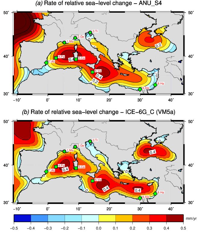
Figure 1: Patterns of the rate of present day sea-level change $\dot{S}$ induced by GIA across the Mediterranean region, according to models ANU$\_$S4 (a) and ICE-6G$\_$C (VM5a) (b). The data in (a) have been obtained from the Datasets page of WR Peltier. In both frames, the locations of a few tide gauges deployed along the coastlines are marked by green symbols. The station names are abbreviated (full names are given in the text and in Table 2).

Table 1: Range of variability for rheological parameters in ensembles E1 and E2, based on nominal models ANU_S4(E1) and ICE-6G (VM5a), respectively. Note that models in ensemble E1 do not include transition zone and shallow lower mantle layers. All models in ensemble E2 assume a $40$ km-thick layer with viscosity $10^{22}\,\mathrm{Pa}\cdot\mathrm{s}$ at the base of the elastic lithosphere. For each ensemble, nominal values of parameters are shown in parentheses.

Ensemble	E1		E2
Nominal model	ANU_S4(E1)		ICE-6G (VM5a)
Lithosphere thickness (km)	$45\div 85$	(65)	$60\div 200$	(100)
Upper mantle viscosity (log, Pa$\cdot$s)	$19.9\div 20.7$	(20.5)	$20.2\div 20.9$	(20.7)
Transition zone viscosity (log, Pa$\cdot$s)	—		$20.5\div 21.2$	(20.7)
Shallow lower mantle viscosity (log, Pa$\cdot$s)	—		$20.7\div 21.5$	(21.2)
Lower mantle viscosity (log, Pa$\cdot$s)	$21.4\div 22.8$	(22.0)	$21.3\div 22.0$	(21.5)

Figure 7: Standard deviation of $\dot{S}$, evaluated varying individual rheological parameters, for the ensemble E1, based upon model ANU_S4(E1). Standard deviations are relative to the nominal model ANU_S4(E1).

Table 2: Rates of relative sea-level change expected at tide gauges according to models ANU_S4 and ICE-6G_C(VM5a), and corresponding averages and 1-$\sigma$ uncertainties according to ensembles E1 and E2. ANU_S4(E1) corresponds to the nominal model of Lambeck & Purcell (2005), upon which Ensemble E1 is based, and it differs from ANU_S4 for the upper mantle viscosity and lithospheric thickness. All rates are in units of $\textrm{mm yr}^{-1}$.

Tide gauge	ANU_S4	ANU_S4(E1)	E1 Ensemble	ICE-6G	E2 Ensemble
1. Marseilles	$+0.08$	$+0.03$	$+0.03\pm 0.08$	$+0.05$	$+0.05\pm 0.03$
2. Genova	$-0.15$	$-0.17$	$-0.16\pm 0.06$	$-0.10$	$-0.10\pm 0.05$
3. Trieste	$-0.20$	$-0.27$	$-0.26\pm 0.06$	$-0.21$	$-0.20\pm 0.07$
4. Palma de Mallorca	$+0.28$	$+0.22$	$+0.21\pm 0.12$	$+0.33$	$+0.33\pm 0.07$
5. Cagliari	$+0.38$	$+0.23$	$+0.20\pm 0.15$	$+0.20$	$+0.20\pm 0.05$
6. Valletta	$+0.33$	$+0.26$	$+0.22\pm 0.16$	$+0.27$	$+0.27\pm 0.06$
7. Alicante I	$-0.03$	$-0.01$	$+0.01\pm 0.06$	$+0.03$	$+0.03\pm 0.03$
8. Hadera	$-0.19$	$-0.15$	$-0.15\pm 0.03$	$-0.05$	$-0.05\pm 0.02$
9. Alexandria	$-0.08$	$-0.10$	$-0.11\pm 0.04$	$-0.07$	$-0.07\pm 0.03$

References

- Amante & Eakins (2009) Amante, C. & Eakins, B., 2009. ETOPO1 Arc-Minute Global Relief Model: Procedures, Data Source and Analysis, Tech. rep.
- Antonioli et al. (2009) Antonioli, F., Ferranti, L., Fontana, A., Amorosi, A., Bondesan, A., Braitenberg, C., Dutton, A., Fontolan, G., Furlani, S., Lambeck, K., et al., 2009. Holocene relative sea-level changes and vertical movements along the italian and istrian coastlines, Quaternary International, 206(1-2), 102–133.
- Anzidei et al. (2014) Anzidei, M., Lambeck, K., Antonioli, F., Furlani, S., Mastronuzzi, G., Serpelloni, E., & Vannucci, G., 2014. Coastal structure, sea-level changes and vertical motion of the land in the Mediterranean, Geological Society, London, Special Publications, 388(1), 453–479.
- Argus et al. (2014) Argus, D. F., Peltier, W., Drummond, R., & Moore, A. W., 2014. The Antarctica component of postglacial rebound model ICE-6G_C (VM5a) based on GPS positioning, exposure age dating of ice thicknesses, and relative sea level histories, Geophysical Journal International, 198(1), 537–563.
- Bernier et al. (1993) Bernier, P., Evin, J., Arnold, M., Pirazzoli, P. A., Montaggioni, L., Laborel, J., Dalongeville, R., & Sanlaville, P., 1993. Les variations recentes de la ligne de rivage sur le littoral syrien, in Quaternaire, vol. 4, 1, 1993.
- Bonaduce et al. (2016) Bonaduce, A., Pinardi, N., Oddo, P., Spada, G., & Larnicol, G., 2016. Sea-level variability in the Mediterranean Sea from altimetry and tide gauges, Climate Dynamics, 47(9), 2851–2866.
- Caron et al. (2018) Caron, L., Ivins, E., Larour, E., Adhikari, S., Nilsson, J., & Blewitt, G., 2018. GIA model statistics for GRACE hydrology, cryosphere, and ocean science, Geophysical Research Letters, 45(5), 2203–2212.
- Cazenave et al. (2002) Cazenave, A., Bonnefond, P., Mercier, F., Dominh, K., & Toumazou, V., 2002. Sea level variations in the Mediterranean Sea and Black Sea from satellite altimetry and tide gauges, Global and Planetary Change, 34(1-2), 59–86.
- Clement et al. (2016) Clement, A. J., Whitehouse, P. L., & Sloss, C. R., 2016. An examination of spatial variability in the timing and magnitude of Holocene relative sea-level changes in the New Zealand archipelago, Quaternary Science Reviews, 131, 73–101.
- Douglas (1991) Douglas, B., 1991. Global sea level rise, Journal of Geophysical Research, 96(C4), 6981–6992.
- Douglas (1997) Douglas, B., 1997. Global sea leve rise: a redetermination, Surveys in Geophysics, 18, 279–292.
- Dziewonski & Anderson (1981) Dziewonski, A. M. & Anderson, D. L., 1981. Preliminary reference Earth model, Physics of the Earth and Planetary Interiors, 25(4), 297–356.
- Eakins & Sharman (2012) Eakins, B. & Sharman, G., 2012. Hypsographic curve of Earth’s surface from ETOPO1, NOAA National Geophysical Data Center, Boulder, CO.
- Evelpidou et al. (2012) Evelpidou, N., Pirazzoli, P., Vassilopoulos, A., Spada, G., Ruggieri, G., & Tomasin, A., 2012. Late Holocene sea level reconstructions based on observations of Roman fish tanks, Tyrrhenian coast of Italy, Geoarchaeology, 27, 259–277.
- Faccenna et al. (2014) Faccenna, C., Becker, T. W., Auer, L., Billi, A., Boschi, L., Brun, J. P., Capitanio, F. A., Funiciello, F., Horvàth, F., Jolivet, L., et al., 2014. Mantle dynamics in the Mediterranean, Reviews of Geophysics, 52(3), 283–332.
- Farrell & Clark (1976) Farrell, W. & Clark, J., 1976. On postglacial sea level, Geophysical Journal International, 46, 647–667.
- Fenoglio-Marc (2002) Fenoglio-Marc, L., 2002. Long-term sea level change in the Mediterranean Sea from multi-satellite altimetry and tide gauges, Physics and Chemistry of the Earth, Parts A/B/C, 27(32-34), 1419–1431.
- Flemming (1978) Flemming, N. C., 1978. Holocene eustatic changes and coastal tectonics in the northeast Mediterranean: implications for models of crustal consumption, Philosophical Transactions of the Royal Society of London. Series A, Mathematical and Physical Sciences, 289(1362), 405–458.
- Fretwell et al. (2013) Fretwell, P., Pritchard, H. D., Vaughan, D. G., Bamber, J. L., Barrand, N. E., Bell, R., Bianchi, C., Bingham, R., Blankenship, D. D., Casassa, G., et al., 2013. Bedmap2: improved ice bed, surface and thickness datasets for Antarctica, The Cryosphere, 7(1), 375–393.
- Galassi & Spada (2014) Galassi, G. & Spada, G., 2014. Sea-level rise in the Mediterranean Sea by 2050: Roles of terrestrial ice melt, steric effects and glacial isostatic adjustment, Global and Planetary Change, 123, 55–66.
- Kachuck & Cathles (2019) Kachuck, S. & Cathles, L. I., 2019. Benchmarked computation of time-domain viscoelastic Love numbers for adiabatic mantles, Geophysical Journal International, 218(3), 2136–2149.
- Kearney (2001) Kearney, M. S., 2001. Late Holocene sea level variation, in Sea level rise: History and consequences, vol. 75, pp. 13–36, International Geophysics Series (75).
- Kierulf et al. (2021) Kierulf, H. P., Steffen, H., Barletta, V. R., Lidberg, M., Johansson, J., Kristiansen, O., & Tarasov, L., 2021. A GNSS velocity field for geophysical applications in Fennoscandia, Journal of Geodynamics, 146, 101845.
- King et al. (2010) King, M. A., Altamimi, Z., Boehm, J., Bos, M., Dach, R., Elosegui, P., Fund, F., Hernández-Pajares, M., Lavallee, D., Cerveira, P. J. M., Penna, N., Riva, R. E., Steigenberger, P., van Dam, T., Vittuari, L., Williams, S., & Willis, P., 2010. Improved constraints on models of glacial isostatic adjustment: a review of the contribution of ground-based geodetic observations, Surveys in Geophysics, 31(5), 465–507.
- Lambeck (1995) Lambeck, K., 1995. Late Pleistocene and Holocene sea-level change in Greece and south-western Turkey: a separation of eustatic, isostatic and tectonic contributions, Geophysical Journal International, 122(3), 1022–1044.
- Lambeck & Purcell (2005) Lambeck, K. & Purcell, A., 2005. Sea-level change in the Mediterranean Sea since the LGM: model predictions for tectonically stable areas, Quaternary Science Reviews, 24(18), 1969–1988.
- Lambeck et al. (2003) Lambeck, K., Purcell, A., Johnston, P., Nakada, M., & Yokoyama, Y., 2003. Water-load definition in the glacio-hydro-isostatic sea-level equation, Quaternary Science Reviews, 22(2), 309–318.
- Lambeck et al. (2004a) Lambeck, K., Antonioli, F., Purcell, A., & Silenzi, S., 2004a. Sea-level change along the Italian coast for the past 10,000 yr, Quaternary Science Reviews, 23(14-15), 1567–1598.
- Lambeck et al. (2004b) Lambeck, K., Anzidei, M., Antonioli, F., Benini, A., & Esposito, A., 2004b. Sea level in Roman time in the Central Mediterranean and implications for recent change, Earth and Planetary Science Letters, 224(3-4), 563–575.
- Lambeck et al. (2017) Lambeck, K., Purcell, A., & Zhao, S., 2017. The North American Late Wisconsin ice sheet and mantle viscosity from glacial rebound analyses, Quaternary Science Reviews, 158, 172–210.
- Li et al. (2020) Li, T., Wu, P., Wang, H., Steffen, H., Khan, N. S., Engelhart, S. E., Vacchi, M., Shaw, T. A., Peltier, W. R., & Horton, B. P., 2020. Uncertainties of glacial isostatic adjustment model predictions in North America associated with 3D structure, Geophysical Research Letters, 47(10), e2020GL087944.
- Love et al. (2016) Love, R., Milne, G. A., Tarasov, L., Engelhart, S. E., Hijma, M. P., Latychev, K., Horton, B. P., & Törnqvist, T. E., 2016. The contribution of glacial isostatic adjustment to projections of sea-level change along the Atlantic and Gulf coasts of North America, Earth’s Future, 4(10), 440–464.
- Martinec et al. (2018) Martinec, Z., Klemann, V., van der Wal, W., Riva, R., Spada, G., Sun, Y., Melini, D., Kachuck, S., Barletta, V., & Simon, K., 2018. A benchmark study of numerical implementations of the sea level equation in GIA modelling, Geophysical Journal International, 215(1), 389–414.
- Mauz et al. (2015) Mauz, B., Ruggieri, G., & Spada, G., 2015. Terminal Antarctic melting inferred from a far-field coastal site, Quaternary Science Reviews, 116, 122–132.
- Melini & Spada (2019) Melini, D. & Spada, G., 2019. Some remarks on Glacial Isostatic Adjustment modelling uncertainties, Geophysical Journal International, 218(1), 401–413.
- Mitrovica & Milne (2002) Mitrovica, J. & Milne, G., 2002. On the origin of late Holocene sea-level highstands within equatorial ocean basins, Quaternary Science Reviews, 21(20), 2179–2190.
- Mitrovica (1996) Mitrovica, J. X., 1996. Haskell [1935] revisited, Journal of Geophysical Research: Solid Earth, 101(B1), 555–569.
- Mitrovica & Peltier (1991) Mitrovica, J. X. & Peltier, W., 1991. On postglacial geoid subsidence over the equatorial oceans, Journal of Geophysical Research: Solid Earth, 96(B12), 20,053–20,071.
- Mitrovica & Wahr (2011) Mitrovica, J. X. & Wahr, J., 2011. Ice Age earth rotation, Annual Review of Earth and Planetary Sciences, 39, 577–616.
- Mitrovica et al. (2005) Mitrovica, J. X., Wahr, J., Matsuyama, I., & Paulson, A., 2005. The rotational stability of an ice-age earth, Geophysical Journal International, 161(2), 491–506.
- Morhange et al. (2006) Morhange, C., Pirazzoli, P. A., Marriner, N., Montaggioni, L. F., & Nammour, T., 2006. Late Holocene relative sea-level changes in Lebanon, Eastern Mediterranean, Marine Geology, 230(1-2), 99–114.
- Murray-Wallace & Woodroffe (2014) Murray-Wallace, C. V. & Woodroffe, C. D., 2014. Quaternary sea-level changes: a global perspective, Cambridge University Press.
- Nakada & Lambeck (1987) Nakada, M. & Lambeck, K., 1987. Glacial rebound and relative sea-level variations: a new appraisal, Geophysical Journal International, 90(1), 171–224.
- Peltier (2004) Peltier, W., 2004. Global glacial isostasy and the surface of the ice-age Earth: the ICE-5G (VM2) model and GRACE, Annu. Rev. Earth Planet. Sci., 32, 111–149.
- Peltier & Andrews (1976) Peltier, W. & Andrews, J., 1976. Glacial-isostatic adjustment I. The forward problem, Geophysical Journal International, 46(3), 605–646.
- Peltier et al. (2015) Peltier, W., Argus, D., & Drummond, R., 2015. Space geodesy constrains ice age terminal deglaciation: The global ICE-6G_C (VM5a) model, Journal of Geophysical Research: Solid Earth, 120(1), 450–487.
- Pirazzoli et al. (1991) Pirazzoli, P., Laborel, J., Saličge, J., Erol, O., Kayan, I., & Person, A., 1991. Holocene raised shorelines on the Hatay coasts (Turkey): palaeoecological and tectonic implications, Marine Geology, 96(3-4), 295–311.
- Pirazzoli (2005) Pirazzoli, P. A., 2005. A review of possible eustatic, isostatic and tectonic contributions in eight late-Holocene relative sea-level histories from the Mediterranean area, Quaternary Science Reviews, 24(18-19), 1989–2001.
- Roy & Peltier (2015) Roy, K. & Peltier, W., 2015. Glacial isostatic adjustment, relative sea level history and mantle viscosity: reconciling relative sea level model predictions for the U.S. East coast with geological constraints, Geophysical Journal International, 201(2), 1156–1181.
- Roy & Peltier (2017) Roy, K. & Peltier, W., 2017. Space-geodetic and water level gauge constraints on continental uplift and tilting over North America: regional convergence of the ICE-6G_C (VM5a/VM6) models, Geophysical Journal International, 210(2), 1115–1142.
- Sanlaville et al. (1997) Sanlaville, P., Dalongeville, R., Bernier, P., & Evin, J., 1997. The syrian coast: A model of holocene coastal evolution, Journal of Coastal Research, 13(2), 385–396.
- Santamaría-Gómez et al. (2017) Santamaría-Gómez, A., Gravelle, M., Dangendorf, S., Marcos, M., Spada, G., & Wöppelmann, G., 2017. Uncertainty of the 20th century sea-level rise due to vertical land motion errors, Earth and Planetary Science Letters, 473, 24–32.
- Sasgen et al. (2012) Sasgen, I., Konrad, H., Ivins, E., van den Broeke, M., Bamber, J., Martinec, Z., & Klemann, V., 2012. Antarctic ice-mass balance 2002 to 2011: regional re-analysis of GRACE satellite gravimetry measurements with improved estimate of glacial-isostatic adjustment, The Cryosphere Discussions, 6(5), 3703–3732.
- Seguinot et al. (2018) Seguinot, J., Ivy-Ochs, S., Jouvet, G., Huss, M., Funk, M., & Preusser, F., 2018. Modelling last glacial cycle ice dynamics in the Alps, The Cryosphere, 12(10), 3265–3285.
- Serpelloni et al. (2013) Serpelloni, E., Faccenna, C., Spada, G., Dong, D., & Williams, S. D., 2013. Vertical GPS ground motion rates in the Euro-Mediterranean region: New evidence of velocity gradients at different spatial scales along the Nubia-Eurasia plate boundary, Journal of Geophysical Research: Solid Earth, 118(11), 6003–6024.
- Simon & Riva (2020) Simon, K. & Riva, R., 2020. Uncertainty estimation in regional models of long-term GIA uplift and sea level change: An overview, Journal of Geophysical Research: Solid Earth, 125(8), e2019JB018983.
- Sivan et al. (2001) Sivan, D., Wdowinski, S., Lambeck, K., Galili, E., & Raban, A., 2001. Holocene sea-level changes along the Mediterranean coast of Israel, based on archaeological observations and numerical model, Palaeogeography, Palaeoclimatology, Palaeoecology, 167(1-2), 101–117.
- Slangen et al. (2012) Slangen, A., Katsman, C., Van de Wal, R., Vermeersen, L., & Riva, R., 2012. Towards regional projections of twenty-first century sea-level change based on IPCC SRES scenarios, Climate dynamics, 38(5-6), 1191–1209.
- Spada (2017) Spada, G., 2017. Glacial Isostatic Adjustment and Contemporary Sea Level Rise: An Overview, Surveys in Geophysics, 38(1), 1–33.
- Spada & Galassi (2012) Spada, G. & Galassi, G., 2012. New estimates of secular sea level rise from tide gauge data and GIA modelling, Geophys. J. Int., 191(3), 1067–1094.
- Spada & Galassi (2015) Spada, G. & Galassi, G., 2015. Spectral analysis of sea-level during the altimetry era, and evidence for GIA and glacial melting fingerprints, Global and Planetary Change, 143, 34–49.
- Spada & Melini (2019a) Spada, G. & Melini, D., 2019a. SELEN4 (SELEN version 4.0): a Fortran program for solving the gravitationally and topographically self-consistent sea-level equation in glacial isostatic adjustment modeling, Geoscientific Model Development, 12(12), 5055–5075.
- Spada & Melini (2019b) Spada, G. & Melini, D., 2019b. On some properties of the Glacial Isostatic Adjustment fingerprints, Water, 11(9), 1844.
- Spada et al. (2011) Spada, G., Barletta, V. R., Klemann, V., Riva, R., Martinec, Z., Gasperini, P., Lund, B., Wolf, D., Vermeersen, L., & King, M., 2011. A benchmark study for glacial isostatic adjustment codes, Geophysical Journal International, 185(1), 106–132.
- Sternai et al. (2019) Sternai, P., Sue, C., Husson, L., Serpelloni, E., Becker, T. W., Willett, S. D., Faccenna, C., Di Giulio, A., Spada, G., Jolivet, L., et al., 2019. Present-day uplift of the European Alps: Evaluating mechanisms and models of their relative contributions, Earth-Science Reviews, 190, 589–604.
- Stocchi & Spada (2007) Stocchi, P. & Spada, G., 2007. Glacio and hydro-isostasy in the Mediterranean Sea: Clark zones and role of remote ice sheets, Annals of Geophysics, 50(6), 741–761.
- Stocchi & Spada (2009) Stocchi, P. & Spada, G., 2009. Influence of glacial isostatic adjustment upon current sea level variations in the Mediterranean, Tectonophysics, 474(1), 56–68.
- Stocchi et al. (2005) Stocchi, P., Spada, G., & Cianetti, S., 2005. Isostatic rebound following the Alpine deglaciation: impact on the sea level variations and vertical movements in the Mediterranean region, Geophysical Journal International, 162(1), 137–147.
- Sun & Riva (2020) Sun, Y. & Riva, R. E. M., 2020. A global semi-empirical glacial isostatic adjustment (GIA) model based on Gravity Recovery and Climate Experiment (GRACE) data, Earth System Dynamics, 11(1), 129–137.
- Tamisiea (2011) Tamisiea, M. E., 2011. Ongoing glacial isostatic contributions to observations of sea level change, Geophysical Journal International, 186(3), 1036–1044.
- Tegmark (1996) Tegmark, M., 1996. An icosahedron-based method for pixelizing the celestial sphere, The Astrophysical Journal, 470, L81.
- Tsimplis et al. (2013) Tsimplis, M., Calafat, F. M., Marcos, M., Jordá, G., Gomis, D., Fenoglio-Marc, L., Struglia, M., Josey, S. A., & Chambers, D., 2013. The effect of the NAO on sea level and on mass changes in the Mediterranean Sea, Journal of Geophysical Research: Oceans, 118(2), 944–952.
- Turcotte & Schubert (2014) Turcotte, D. L. & Schubert, G., 2014. Geodynamics - Applications of Continuum Physics to Geological Problems, Cambridge University Press.
- Tushingham & Peltier (1991) Tushingham, A. & Peltier, W., 1991. ICE-3G – A new global model of late Pleistocene deglaciation based upon geophysical predictions of post-glacial relative sea level change, Journal of Geophysical Research, 96(B3), 4497–4523.
- Tushingham & Peltier (1992) Tushingham, A. & Peltier, W., 1992. Validation of the ICE-3G model of Würm-Wisconsin deglaciation using a global data base of relative sea level histories, Journal of Geophysical Research, 97(B3), 3285–3304.
- Vacchi et al. (2016) Vacchi, M., Marriner, N., Morhange, C., Spada, G., Fontana, A., & Rovere, A., 2016. Multiproxy assessment of Holocene relative sea-level changes in the western Mediterranean: Sea-level variability and improvements in the definition of the isostatic signal, Earth-Science Reviews, 155, 172–197.
- Vacchi et al. (2018) Vacchi, M., Ghilardi, M., Melis, R., Spada, G., Giaime, M., Marriner, N., Lorscheid, T., Morhange, C., Burjachs, F., & Rovere, A., 2018. New relative sea-level insights into the isostatic history of the Western Mediterranean, Quaternary Science Reviews, 201, 396–408.
- Vestøl et al. (2019) Vestøl, O., Ågren, J., Steffen, H., Kierulf, H., & Tarasov, L., 2019. NKG2016LU: a new land uplift model for Fennoscandia and the Baltic Region, Journal of Geodesy, 93(9), 1759–1779.
- Walcott (1972) Walcott, R., 1972. Past sea levels, eustasy and deformation of the earth, Quaternary Research, 2(1), 1–14.
- Whitehouse (2018) Whitehouse, P. L., 2018. Glacial isostatic adjustment modelling: historical perspectives, recent advances, and future directions, Earth Surface Dynamics, 6(2), 401–429.
- Woodworth (2003) Woodworth, P. L., 2003. Some comments on the long sea level records from the northern Mediterranean, Journal of Coastal Research, pp. 212–217.