Kittel’s molecular zipper model on Cayley trees

Abstract.

Kittel’s 1D model represents a natural DNA with two strands as a (molecular) zipper, which may separated as the temperature is varied. We define multidimensional version of this model on a Cayley tree and study the set of Gibbs measures. We reduce description of Gibbs measures to solving of a non-linear functional equation, with unknown functions (called boundary laws) defined on vertices of the Cayley tree. Each boundary law defines a Gibbs measure. We give general formula of free energy depending on the boundary law. Moreover, we find some concrete boundary laws and corresponding Gibbs measures. Explicit critical temperature for occurrence a phase transition (non-uniqueness of Gibbs measures) is obtained.

Mathematics Subject Classifications (2010). 92D20; 82B20; 60J10.

Key words. Cayley tree, configuration, Gibbs measure, phase transition, zipper model.

1. Introduction

One of classical results is that there cannot be phase transitions in 1D systems with short range interactions. As noted in [3], this assertion is often receives the name “van Hove’s theorem” [6], but van Hove proved it for a system of hard-core segments of a diameter $d_{0}$, that interact only at distances smaller than $d_{1}$ and assuming that the interaction potential is a continuous, bounded below function. This result was generalized by Ruelle [12].

At the same time some models (Kittel’s model, Chui-Weeks’s model, Dauxois-Peyrard’s model) were found with phase transitions in spite of their 1D character and the range of their interactions (see [3] for details).

In this paper we are going to study Kittel’s model on a Cayley tree of arbitrary order $k\geq 1$. Note that for $k=1$ this tree coincides with 1D integer lattice $\mathbb{Z}^{1}$.

We are interested to the set of Gibbs measures (in particular to problems of phase transitions) for the Kittel’s model on trees.

1D Kittel’s model is defined as follows (see [3], [5]). Consider a single-ended zipper of $N$ links that can be opened only from one end. This zipper is model of a natural DNA (see [1] for structure of a DNA) two strands of which may separated as the temperature is varied (see Fig. 1).

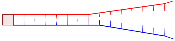
Figure 1. Single-ended zipper (DNA) with some open and closed links.

If links $1,2,...,n$ are all open, the energy required to open link $n+1$ is $\epsilon$. However, if all the preceding links are not open, the energy required to open link $n+1$ is infinite. The link $N$ (the end) cannot be opened, and the zipper is said to be open when the first $N-1$ links are open. Suppose that there are $q$ orientations which each open link can assume, i.e., the open state of a link is $q$-fold degenerated.

In [3] the 1D Kittel’s model in solved in terms of a transfer matrix for the model’s Hamiltonian defined as

$$H_{N}(s)=\epsilon\left(1-\delta_{0,s_{1}}\right)+\sum_{i=2}^{N-1}\left(\epsilon+J\delta_{0,s_{i-1}}\right)\left(1-\delta_{0,s_{i}}\right),$$ (1.1)

where $s\in\{0,1,\dots,q\}^{N}$, $s_{i}=0$ means that link $i$ is closed, $s_{i}=1,2,\ldots,q$ means that the link is open in one of the possible $q$ states, and $\delta_{s,s^{\prime}}$ is the Kronecker symbol.

Kittel assumed that $J=\infty$, and the boundary condition $s_{N}=0$ (the leftmost end of the zipper is always closed). The partition function is given by

$$Z_{N}=\sum_{s\in\{0,1,\dots,q\}^{N}:\atop s_{N}=0}\exp\left(-\beta H_{N}(s)\right),$$

with $\beta=1/T$ is the inverse temperature.

For the case $J=\infty$ by Kittel it was obtained that

$$Z_{N}={1-a^{N}\over 1-a},\ \ \mbox{where}\ \ a=q\exp(-\beta\epsilon).$$

In order to have a phase transition, meaning a non-analyticity of the free energy, one can see that at $T_{c}={\epsilon\over\ln q}$, the derivative of the free energy is discontinuous. Moreover, note that $T_{c}$ is finite iff $q>1$; for the non-degenerate case $q=1$ (only one open state) there is no phase transition.

In this paper we consider Kittel’s model on the Cayley tree of arbitrary order $k\geq 1$. This model pretenses a set of interacting DNAs as introduced in [7], [8], [9]. Note that the case $k=1$ coincides with 1D case, i.e., original Kittel’s model.

The paper is organized as follows. In Section 2 we give main definitions. In Section 3 we reduce description of Gibbs measures of the Kittel’s model to solving a non-linear functional equation, with unknown functions defined on vertices of the Cayley tree. Such a function is called a boundary law (see [4, chapter 12] and [2, section 1.2.4]). Each boundary law defines a Gibbs measure. In Section 4, for each boundary law, we give formula of corresponding free energy. Sections 5 and 6 are devoted to finding concrete boundary laws (and corresponding Gibbs measures). We find explicitly critical temperature of occurrence of phase transitions (non-uniqueness of Gibbs measures).

2. Preliminaries

For convenience of a reader let us recall some definitions (see [7]).

Cayley tree. The Cayley tree $\Gamma^{k}$ of order $k\geq 1$ is an infinite tree, i.e., a graph without cycles, such that exactly $k+1$ edges originate from each vertex. Let $\Gamma^{k}=(V,L,i)$, where $V$ is the set of vertices $\Gamma^{k}$, $L$ the set of edges and $i$ is the incidence function setting each edge $l\in L$ into correspondence with its endpoints $x,y\in V$. If $i(l)=\{x,y\}$, then the vertices $x$ and $y$ are called the nearest neighbors, denoted by $l=\langle x,y\rangle$.

If an arbitrary edge $\langle x^{0},x^{1}\rangle=l\in L$ is deleted from the Cayley tree $\Gamma^{k}$, it splits into two components, i.e., two identical semi-infinite trees $\Gamma^{k}_{0}$ and $\Gamma^{k}_{1}$ (see Fig. 2).

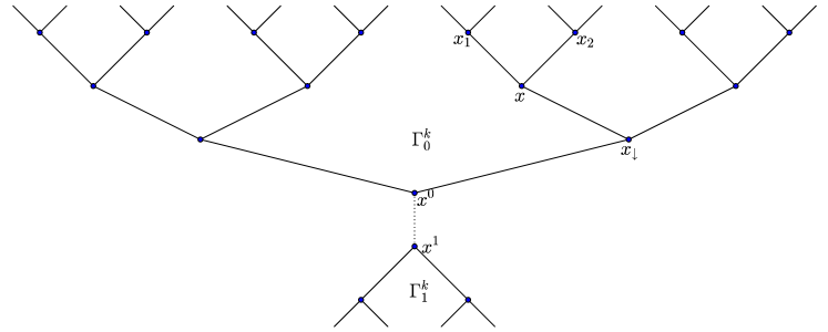
Figure 2. The Cayley tree of order $k=2$, separated to two semi-infinite sub-trees $\Gamma^{k}_{0}$ and $\Gamma^{k}_{1}$. Shown an example of $x$, $x_{\downarrow}$ and $S(x)=\{x_{1},x_{2}\}$.

In this paper we consider semi-infinite Cayley tree $\Gamma^{k}_{0}=(V_{0},L_{0})$. The vertex $x^{0}$ is considered as a root of tree, the root has $k$ nearest neighbors and all other vertices of $\Gamma^{k}_{0}$ has $k+1$ nearest neighbors.

Denote by $S_{1}(x)$ the set of all nearest neighbors of $x\in V_{0}$. Let $x_{\downarrow}$ be unique vertex in $S_{1}(x)$ (where $x\in V_{0}\setminus\{x^{0}\}$) which is closer to $x^{0}$ than other elements of $S_{1}(x)$. Denote also

$$S(x)=S_{1}(x)\setminus\{x_{\downarrow}\}.$$

The distance $d(x,y),x,y\in V_{0}$ on the Cayley tree is the number of edges of the shortest path from $x$ to $y$:

$$d(x,y)=\min\{d\,|\,\exists x=x_{0},x_{1},\dots,x_{d-1},x_{d}=y\in V_{0}\ \ \mbox{such that}\ \ \langle x_{0},x_{1}\rangle,\dots,\langle x_{d-1},x_{d}\rangle\}.$$

For the fixed $x^{0}\in V$ (the above defined root) and $n\geq 1$ we set

$$|x|=d(x,x^{0}),\ \ W_{n}=\ \{x\in V_{0}\ \ |\ \ |x|=n\},$$

$$V_{n}=\ \{x\in V_{0}\ \ |\ \ |x|\leq n\},\ \ L_{n}=\ \{l=\langle x,y\rangle\in L\ |\ x,y\in V_{n}\}.$$ (2.1)

Configuration space. Consider spin values from $\Phi=\{0,1,\dots,q\}$, where $q\geq 1$.

A configuration is any mapping $\sigma:x\in V\to\sigma(x)\in\Phi$. The vertex $x$ with $\sigma(x)=0$ means that the vertex is closed. Each $\sigma(x)=1,2,\dots q$ means that the vertex $x$ is open in one of possible $q$ states.

For any $x\in V_{0}$ denote by $\pi_{x}$ the unique path connection $x^{0}$ and $x$.

Definition 1.

A configuration $\sigma\in\Omega$ is called zipper-admissible if $\sigma(x^{0})=0$ and from $\sigma(x)=0$ it follows that $\sigma(y)=0$ for all $y\in\pi_{x}$ (see Fig. 3).

In this paper we only consider zipper-admissible configurations. Denote by $\Omega=\Phi^{V_{0}}$ the set of all such configurations.

Admissible configurations in $V_{n}$ are defined analogously and the set of all such configurations is denoted by $\Omega_{n}$.

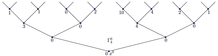
Figure 3. An example of zipper-admissible configuration on the Cayley tree of order $k=2$, with $q\geq 10$.

The Hamiltonian of zipper model. We consider the following model of the energy of the zipper-admissible configuration $\sigma\in\Omega$ :

$$H(\sigma)=\epsilon\sum_{x\in W_{1}}(1-\delta_{0,\sigma(x)})+\sum_{x\in V_{0}\setminus V_{1}}\left(\epsilon+J\delta_{0,\sigma(x_{\downarrow})}\right)\left(1-\delta_{0,\sigma(x)}\right),$$ (2.2)

where $\epsilon\in\mathbb{R}$, $J\in\mathbb{R}\cup\{\infty\}$ are parameters, $\delta$ is the Kronecker delta.

Remark 1.

We note that Hamiltonian (2.2) generalizes (1.1) (firstly given in [3]) from $k=1$ to $k\geq 1$ and Kittel’s model from $J=+\infty$ to $J\in\mathbb{R}\cup\{\infty\}$.

3. System of functional equations of finite dimensional distributions

Let $\Omega_{n}$ be the set of all zipper-admissible configurations on $V_{n}$.

Define a finite-dimensional distribution of a probability measure $\mu$ on $\Omega_{n}$ as

$$\mu_{n}(\sigma_{n})=Z_{n}^{-1}\exp\left\{-\beta H_{n}(\sigma_{n})+\sum_{y\in W_{n}}h_{\sigma(y),y}\right\},$$ (3.1)

where $\sigma_{n}\in\Omega_{n}$, $\beta=1/T$, $T>0$ is temperature, $Z_{n}^{-1}$ is the normalizing factor (partition function):

$$Z_{n}:=Z_{n}(\beta,h)=\sum_{\hat{\sigma}_{n}\in\Omega_{n}}\exp\left\{-\beta H_{n}(\hat{\sigma}_{n})+\sum_{y\in W_{n}}h_{\hat{\sigma}(y),y}\right\},$$ (3.2)

and

$$\{h_{a,x}\in\mathbb{R}:\,a\in\Phi,\,x\in V_{0}\}$$

is a collection of real numbers and

$$H_{n}(\sigma_{n})=\epsilon\sum_{x\in W_{1}}(1-\delta_{0,\sigma(x)})+\sum_{x\in V_{n}\setminus V_{1}}\left(\epsilon+J\delta_{0,\sigma(x_{\downarrow})}\right)\left(1-\delta_{0,\sigma(x)}\right).$$

We say that the probability distributions (3.1) are compatible if for all $n\geq 1$ and $s_{n-1}\in\Omega_{n-1}$:

$$\sum_{\omega_{n}\in\Omega_{W_{n}}}\mu_{n}(s_{n-1}\vee\omega_{n})=\mu_{n-1}(s_{n-1}).$$ (3.3)

Here $s_{n-1}\vee\omega_{n}$ is the concatenation of the configurations.

The following theorem gives a criterion for compatibility of finite-dimensional distributions.

Theorem 1.

Probability distributions $\mu_{n}(\sigma_{n})$, $n=1,2,\ldots$, in (3.1) are compatible iff for any $x\in V_{0}\setminus\{x^{0}\}$ the following equation holds:

$$z_{x}=\prod_{y\in S(x)}\left(\theta z_{y}+\eta\right),$$ (3.4)

where $\theta={1\over q}\exp(\beta\epsilon)$, $\eta=\exp(-\beta J)$, and $z_{x}=\exp(h_{0,x}-h_{i,x})$ (independent on $i=1,\dots,q$).

Proof.

Necessity. Suppose that (3.3) holds; we want to prove (3.4). Substituting (3.1) into (3.3), for any $n\geq 2$ and configurations $\sigma_{n-1}$: $x\in V_{n-1}\mapsto\sigma_{n-1}(x)\in\Phi$ we obtain

$$\begin{array}[]{ll}\frac{Z_{n-1}}{Z_{n}}\sum_{\omega_{n}\in\Omega_{W_{n}}}\exp\left[\sum_{x\in W_{n-1}}\sum_{y\in S(x)}\left\{-\beta\left(\epsilon+J\delta_{0,\sigma_{n-1}(x)}\right)\left(1-\delta_{0,\omega_{n}(y)}\right)+h_{\omega_{n}(y),y}\right\}\right]=\\[5.69054pt] \exp\left(\sum_{x\in W_{n-1}}h_{\sigma_{n-1}(x),x}\right),\end{array}$$ (3.5)

where $\omega_{n}$: $x\in W_{n}\mapsto\omega_{n}(x)$.

From (3.5) we get:

$${Z_{n-1}\over Z_{n}}\sum_{\omega_{n}\in\Omega_{W_{n}}}\prod_{x\in W_{n-1}}\prod_{y\in S(x)}\exp\left[-\beta\left(\epsilon+J\delta_{0,\sigma_{n-1}(x)}\right)\left(1-\delta_{0,\omega_{n}(y)}\right)+h_{\omega_{n}(y),y}\right]=$$

$$\prod_{x\in W_{n-1}}\exp\,(h_{\sigma_{n-1}(x),x}).$$ (3.6)

Fix $x\in W_{n-1}$, $n\geq 2$ and consider two configurations $\sigma_{n-1}=\overline{\sigma}_{n-1}$ and $\sigma_{n-1}=\tilde{\sigma}_{n-1}$ on $W_{n-1}$ which coincide on $W_{n-1}\setminus\{x\}$, and rewrite the equality (3.6) for $\overline{\sigma}_{n-1}(x)=0$, and $\tilde{\sigma}_{n-1}(x)=i$ (where $i=1,\dots,q$), then dividing first of them to the second one we get

$$\exp\,(h_{0,x}-h_{i,x})=\prod_{y\in S(x)}\frac{\sum_{j\in\Phi}\exp\left[-\beta(\epsilon+J)\left(1-\delta_{0,j}\right)+h_{j,y}\right]}{\sum_{j\in\Phi\setminus\{0\}}\exp\left[-\beta\epsilon\left(1-\delta_{0,j}\right)+h_{j,y}\right]}$$

$$=\prod_{y\in S(x)}\frac{e^{h_{0,y}}+\sum_{j=1}^{q}e^{-\beta(\epsilon+J)+h_{j,y}}}{\sum_{j=1}^{q}e^{-\beta\epsilon+h_{j,y}}}.$$ (3.7)

From this equality we note that $z_{i,x}=\exp(h_{0,x}-h_{i,x})$ must be independent on $i=1,\dots,q$. Therefore we introduce $z_{x}\equiv z_{i,x}$. Then from (3.7) we get (3.4).

Sufficiency. Suppose that (3.4) holds. It is equivalent to the representations

$$\begin{array}[]{ll}\prod_{y\in S(x)}\sum_{j\in\Phi}\exp\left[-\beta(\epsilon+J)\left(1-\delta_{0,j}\right)+h_{j,y}\right]=a(x)\exp\,(h_{0,x}),\\[8.53581pt] \prod_{y\in S(x)}\sum_{j\in\Phi\setminus\{0\}}\exp\left[-\beta\epsilon\left(1-\delta_{0,j}\right)+h_{j,y}\right]=a(x)\exp\,(h_{i,x}),i\in\Phi\setminus\{0\}\end{array}$$ (3.8)

for some function $a(x)>0,x\in V_{0}\setminus\{x^{0}\}.$ We have

$${\rm LHS\ \ of\ \ (\ref{**})}=\frac{1}{Z_{n}}\exp(-\beta H(\sigma_{n-1}))\times$$ (3.9)

$$\prod_{x\in W_{n-1}}\prod_{y\in S(x)}\sum_{j\in\Phi}\exp\left[-\beta(\epsilon+J\delta_{0,\sigma_{n-1}(x)})\left(1-\delta_{0,j}\right)+h_{j,y}\right].$$

Substituting (3.8) into (3.9) and denoting $A_{n}(x)=\prod_{x\in W_{n-1}}a(x)$, we get

$${\rm RHS\ \ of\ \ (\ref{ru1})}=\frac{A_{n-1}}{Z_{n}}\exp(-\beta H(\sigma_{n-1}))\prod_{x\in W_{n-1}}\exp(h_{\sigma_{n-1}(x),x}).$$ (3.10)

Since $\mu^{(n)}$, $n\geq 2$ is a probability, we should have

$$\sum_{\sigma_{n-1}\in\Omega_{V_{n-1}}}\sum_{\omega_{n}\in\Omega_{W_{n}}}\mu^{(n)}(\sigma_{n-1},\omega_{n})=1.$$

Hence from (3.10) we get $Z_{n-1}A_{n-1}=Z_{n}$, and (3.3) holds. ∎

By this theorem the problem of description of Gibbs measures is reduced to the problem of solving the functional equation (3.4). It is difficult to describe all solutions of this equation. Below under some conditions on parameters of the model we find several solutions.

Remark 2.

From the proof of Theorem 1 we know that $z_{x}=\exp(h_{0,x}-h_{i,x})$ must be independent on $i=1,\dots,q$, i.e., $h_{1,x}=\dots=h_{q,x}$. Moreover, for each $x\in V_{0}\setminus\{x^{0}\}$ adding a number $\alpha_{x}$ to both $h_{0,x}$ and $h_{i,x}$ does not change the value $h_{0,x}-h_{i,x}$. Thus without loss of generality we can assume that $h_{0,x}+h_{1,x}=0$ for any $x$. Indeed, if $h_{0,x}+h_{1,x}\neq 0$ we consider new functions $\hat{h}_{0,x}=h_{0,x}+\alpha_{x}$ and $\hat{h}_{i,x}=h_{1,x}+\alpha_{x}$ where $\alpha_{x}={-1\over 2}(h_{0,x}+h_{1,x})$. Then

$$z_{x}=\exp(h_{0,x}-h_{i,x})=\exp(\hat{h}_{0,x}-\hat{h}_{i,x}),$$

with $\hat{h}_{0,x}+\hat{h}_{i,x}=0$.

A solution $z_{x}=\exp(h_{0,x}-h_{1,x})$ satisfying (3.4) and $h_{0,x}+h_{1,x}=0$ will be in the sequel called compatible.

4. Free energy

Recall that a reduced free energy is

$$f_{n}(\beta,h)={1\over|V_{n}|}\cdot\ln Z_{n}(\beta,h),$$

where $Z_{n}(\beta,h)$ is defined in (3.2).

It is known that the reduced free energy encodes the relevant information about the physical system; for example, its first derivative with respect to $\beta$ yields the internal energy while its second derivative yields, up to a multiplicative prefactor, the specific heat. For a finite volume, this is a (real) analytic function in $\beta$. But some failures of analyticity can only occur in the infinite volume limit:

$$f(\beta,h)=\lim_{n\to\infty}{1\over|V_{n}|}\cdot\ln Z_{n}(\beta,h).$$

If the resulting limit of the reduced free energy is an analytic function of $\beta$ (equivalently, temperature), then the model has no (finite-temperature) phase transition. Finite values of $\beta$, or equivalently $T$, where analyticity fails are finite temperature critical points corresponding to phase transitions.

For models given on a Cayley tree the free energy also depends on boundary law, i.e., solutions of equation (3.4) (see [11] and references therein).

Theorem 2.

For compatible solution of (3.4), the free energy is given by the formula

$$f(\beta,h)=\lim_{n\to\infty}\frac{1}{|V_{n}|}\sum_{x\in V_{n}}b(x),$$ (4.1)

where

$$b(x)=\frac{1}{2}\ln\left({\theta z_{x}+\eta\over\theta^{2}z_{x}}\right).$$

Proof.

By definitions (1.1), (3.2) we take initial value

$$Z_{1}(\beta,h)=\sum_{\sigma\in\Omega_{1}}\prod_{x\in W_{1}}\exp\left\{-\beta\epsilon(1-\delta_{0,\sigma(x)})+h_{\sigma(x),x}\right\},$$ (4.2)

and use the following recurrent formula (see the last line in the proof of Theorem 1):

$$Z_{n}(\beta,h)=A_{n-1}Z_{n-1}(\beta,h),\ \ n\geq 2$$ (4.3)

where $A_{n}=\prod\limits_{x\in W_{n}}a(x)$ with some function $a(x)>0,x\in V\setminus\{x^{0}\}$ satisfying

$$\begin{array}[]{ll}\prod_{y\in S(x)}\sum_{j\in\Phi}\exp\left[-\beta(\epsilon+J)\left(1-\delta_{0,j}\right)+h_{j,y}\right]=a(x)\exp\,(h_{0,x}),\\[8.53581pt] \prod_{y\in S(x)}\sum_{j\in\Phi\setminus\{0\}}\exp\left[-\beta\epsilon\left(1-\delta_{0,j}\right)+h_{j,y}\right]=a(x)\exp\,(h_{1,x}).\end{array}$$ (4.4)

Multiply these equalities and using $h_{0,x}+h_{1,x}=0$ (i.e., $z_{x}=\exp(-2h_{1,x})$) we obtain

$$a(x)=\theta^{-k}\prod_{y\in S(x)}\left[z^{-1}_{y}(\theta z_{y}+\eta)\right]^{1/2}=\exp\Big{(}\sum_{y\in S(x)}b(y)\Big{)}=\prod_{y\in S(x)}\exp(b(y)).$$

Inserting this formula into the recursive equation (4.3) and by iteration we get

$$Z_{n}(\beta,h)=\prod_{x\in V_{n-1}}a(x)=\prod_{x\in V_{n-1}}\prod_{y\in S(x)}\exp(b(y))=\prod_{x\in V_{n}}\exp(b(x)),\ \ n\geq 2,$$

which gives (4.1). ∎

5. Case $J=\infty$

In this case $\eta=0$ and the functional equation (3.4) is reduced to

$$z_{x}=\theta^{k}\prod_{y\in S(x)}z_{y}.$$ (5.1)

Sub-case: $k=1$. In this case we can identify vertices of $\Gamma_{0}^{1}$ as elements of $\mathbb{N}_{0}=\{0,1,2\dots\}$. Therefore the functional equation is reduced to

$$z_{n}=\theta z_{n+1}\ \ \Leftrightarrow\ \ z_{n+1}={z_{n}\over\theta},\ \ z_{1}>0,\,n\geq 1.$$

Consequently

$$z_{n}=\theta^{-(n-1)}z_{1},\ \ n\geq 1.$$

This is general solution of (5.1) for the case $k=1$.

Sub-case: $k\geq 2$. In this case we give a family of solutions. To do this we assume that a solution $z_{x}$ depends on $|x|$ but not on $x$ itself, i.e., such a solution is in the form

$$0<z_{x}=a_{n}\equiv a_{n}(\theta,k),\ \ \mbox{where}\ \ n=|x|\in\{1,2,\dots\}.$$

Since $a_{n}>0$ and $\theta>0$ with $\theta\neq 1$ we can introduce $\alpha_{n}=\log_{\theta}a_{n}$. For arbitrary $\alpha_{1}\in\mathbb{R}$ define

$$\alpha_{n}={1\over k^{n}}\left(\alpha_{1}-{k(k^{n}-1)\over k-1}\right),\ \ n\geq 2.$$ (5.2)

Proposition 1.

Let $k\geq 2$ and $\alpha_{n}$ be as in (5.2) then $z_{x}=\theta^{\alpha_{|x|}}$, $x\in V_{0}\setminus\{x^{0}\}$ is a solution to (5.1) for any $\alpha_{1}\in\mathbb{R}$.

Proof.

Let $z_{x}=\theta^{\alpha_{|x|}}$ be a solution of (5.1) we show that $\alpha_{n}$ is as in (5.2). If $|x|=n$ then for any $y\in S(x)$ we have $|y|=|x|+1=n+1$. Therefore, from (5.1) we get

$$\alpha_{|x|}=k\left(\alpha_{|x|+1}+1\right),\ \ \mbox{i.e.}\ \ \alpha_{n+1}={\alpha_{n}\over k}-1,\,n\geq 1.$$

It is easy to see that this recurrent formula gives (5.2). Moreover, with this $\alpha_{|x|}$ the function $z_{x}=\theta^{\alpha_{|x|}}$ satisfies (5.1). ∎

Remark 3.

We note that the functional equation (5.1) has constant solution:

$$z_{x}=z^{*}=\theta^{-{k\over k-1}},\ \ \forall x\in V_{0}\setminus\{x^{0}\}.$$

Moreover, since $\lim_{n\to\infty}\alpha_{n}=-{k\over k-1}$ we have $\lim_{|x|\to\infty}z_{x}=z^{*}$ independently on $\alpha_{1}\in\mathbb{R}$.

Remark 4.

For case $\eta=0$ the free energy is independent on solutions (see (4.1)). Derivative of the free energy at $\theta=1$ (i.e. $T_{c}={\epsilon\over\ln q}$) is discontinuous. This generalizes Kittel’s result, for $k\geq 1$, meaning a phase transition.

By Theorem 1 to each above mentioned solution corresponds a Gibbs measure, which we denote by $\mu_{z_{1}}$ (where $z_{1}>0$ for $k=1$ and $z_{1}=\theta^{\alpha_{1}}$ for $k\geq 2$) and $\mu_{z^{*}}$.

We note that in case $\theta=1$ all measures coincide (because the solutions coincide). Moreover, by formula (3.1) one can see that $\mu_{z_{1}}=\mu_{z^{\prime}_{1}}$ iff $z_{1}=z^{\prime}_{1}$.

Summarizing we obtain

Theorem 3.

For any $k\geq 1$ and $\theta>0$, $\theta\neq 1$ there are uncountable many Gibbs measures $\mu_{z^{*}}$, $\mu_{z_{1}}$, $z_{1}>0$.

Remark 5.

Theorem 3 gives another view on the phase transition phenomenon: at critical value $\theta=1$ (i.e. $T_{c}={\epsilon\over\ln q}$) there is unique Gibbs measure; but for $T\neq T_{c}$ there are uncountable Gibbs measures. Thus uniqueness only at one temperature, this is quit different phenomenon compared with classical models (on Cayley trees) such as Ising model (see [10] and references therein) and Potts model (see [7]), where uniqueness of Gibbs measure holds for a continuous infinite region of temperature but there are uncountable measures as soon as a phase transition occurs.

6. Constant solutions for $J<+\infty$

In this section, for $J\neq\infty$ we solve (3.4) in class of constant functions, i.e., assume $z_{x}\equiv z$. Then we get

$$z=\left(\theta z+\eta\right)^{k}.$$ (6.1)

By definitions of parameters we have $\theta>0$, $\eta>0$ and $z>0$. Full analysis of equation (6.1) given in the following lemma

Lemma 1.

For $k\geq 2$, let $N_{k}(\theta,\eta)$ be the number of positive solutions ($z>0$) of (6.1). It has the following form

$$N_{k}(\theta,\eta)=\left\{\begin{array}[]{lll}0,\ \ \mbox{if}\ \ \eta>\eta_{c}\\[5.69054pt] 1,\ \ \mbox{if}\ \ \eta=\eta_{c}\\[5.69054pt] 2,\ \ \mbox{if}\ \ 0<\eta<\eta_{c},\end{array}\right.$$

where $\eta_{c}\equiv\eta_{c}(k,\theta):={k-1\over k\sqrt[k-1]{k\theta}}.$

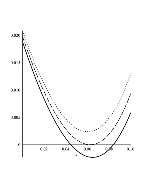
Figure 4. Plots of $f_{4}(z,2,\eta)$ for $\eta>\eta_{c}=3/8$ doted curve; for $\eta=\eta_{c}$ dashed curve; for $\eta<\eta_{c}$ solid curve.

Proof.

Define

$$f_{k}(z,\theta,\eta):=\left(\theta z+\eta\right)^{k}-z.$$

We have

$$f_{k}(0,\theta,\eta)=\eta^{k}>0,\ \ f_{k}(+\infty,\theta,\eta)=+\infty,$$

$${\partial\over\partial z}f_{k}(z,\theta,\eta):=k\theta\left(\theta z+\eta\right)^{k-1}-1=0\ \ \Leftrightarrow\ \ z=z^{*}:={1\over\theta}\left({1\over\sqrt[k-1]{k\theta}}-\eta\right).$$

Thus $f_{k}(z,\theta,\eta)$ is monotone decreasing if $0<z\leq z^{*}$ and increasing if $z>z^{*}$. Moreover,

$$z^{*}>0\ \ \Leftrightarrow\ \ \eta<{1\over\sqrt[k-1]{k\theta}}.$$ (6.2)

Under condition (6.2) we have

$$\min_{z\geq 0}f_{k}(z,\theta,\eta)=f_{k}(z^{*},\theta,\eta)={1\over\theta}\left(\eta-{k-1\over k\sqrt[k-1]{k\theta}}\right).$$

Therefore equation (6.1) does not have a positive solution if $\min_{z\geq 0}f_{k}(z,\theta,\eta)>0$; it has unique positive solution if $\min_{z\geq 0}f_{k}(z,\theta,\eta)=0$ and it has exactly two solutions if $\min_{z\geq 0}f_{k}(z,\theta,\eta)<0$ (see Fig.4). This completes the proof. ∎

By this lemma, if $\eta<\eta_{c}$ (resp. $\eta=\eta_{c}$) then there are exactly two (resp. one ) solutions to (6.1), denote them by $z_{1}$ and $z_{2}$ (resp. $z_{1}$). Let $\mu_{i}$ be translation invariant Gibbs measure (TIGM) corresponding (by Theorem 1) to solution $z_{x}\equiv z_{i}$, $i=1,2$. From Lemma 1 by Theorem 1 we get the following

Theorem 4.

Let $N_{TIGM}(k,\theta,\eta)$ denote the number of TIGMs of the Kittel’s model (where $\eta>0$). Then

$$N_{TIGM}(k,\theta,\eta)=\left\{\begin{array}[]{lll}0,\ \ \mbox{if}\ \ \eta>\eta_{c}\\[5.69054pt] 1,\ \ \mbox{if}\ \ \eta=\eta_{c}\\[5.69054pt] 2,\ \ \mbox{if}\ \ \eta<\eta_{c}.\end{array}\right.$$

Using $\theta={1\over q}\exp(\beta\epsilon)$, $\eta=\exp(-\beta J)$, $\beta=1/T$ from equation $\eta=\eta_{c}$, with respect to $T>0$, we get the following critical temperature

$$T_{\rm cr}\equiv T_{\rm cr}(k,q,\epsilon,J)={\epsilon-(k-1)J\over\ln\left(q\,{(k-1)^{k-1}\over k^{k}}\right)}.$$ (6.3)

Consider the following set

$$A=\{(k,q,\epsilon,J)\in\mathbb{N}^{2}\times\mathbb{R}^{2}\,:\,T_{\rm cr}(k,q,\epsilon,J)>0\}.$$

From Theorem 4 we get

Corollary 1.

For the Kittel’s model on the Cayley tree of order $k\geq 1$, if $(k,q,\epsilon,J)\in A$ then there is a phase transition. Moreover, non-uniqueness of Gibbs measure holds for $T<T_{\rm cr}$ (resp. $T>T_{\rm cr}$) if $J>0$ (resp. $J<0$).

Example. Consider the case $k=2$, i.e., Cayley tree of order two. In this case two solutions mentioned in Lemma 1 can be found explicitly:

$$z_{\pm}:={1-2\theta\eta\pm\sqrt{1-4\theta\eta}\over 2\theta^{2}}.$$

Here $\eta<\eta_{c}={1\over 4\theta}$, i.e., $T_{\rm cr}={\epsilon-J\over\ln(q/4)}$. Corresponding free energies are

$$f(\beta,z_{\pm})=-{1\over 4}\ln(\theta^{4}z_{\pm}).$$

In Fig.5 we give graphs of the free energies.

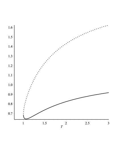
Figure 5. Graphs of free energy $f({1\over T},z_{+})$ (the solid line) and $f({1\over T},z_{-})$ (the doted line) on $1=T_{\rm cr}\leq T\leq 3$ in case $k=2$, $q=8$, $\epsilon=2\ln 2$, $J=\ln 2$.

Statements and Declarations

Conflict of interest statement: The author states that there is no conflict of interest.

Data availability statements

The datasets generated during and/or analyzed during the current study are available from the author on reasonable request.

References

- [1] B. Alberts, A. Johnson, J. Lewis, M. Raff, K. Roberts, and P. Walter, Molecular Biology of the Cell. 4th edition. New York: Garland Science; 2002.
- [2] L.V. Bogachev, U.A. Rozikov, On the uniqueness of Gibbs measure in the Potts model on a Cayley tree with external field. J. Stat. Mech. Theory Exp. (2019), no. 7, 073205, 76 pp.
- [3] J.A. Cuesta, A. Sánchez, General Non-Existence Theorem for Phase Transitions in One-Dimensional Systems with Short Range Interactions, and Physical Examples of Such Transitions. J. Stat. Phys. 115(3/4), (2004), 869-893.
- [4] H.O. Georgii, Gibbs Measures and Phase Transitions, Second edition. de Gruyter Studies in Mathematics, 9. Walter de Gruyter, Berlin, 2011.
- [5] C. Kittel, Phase Transition of a Molecular Zipper. Am. J. Phys. 37(9), (1969), 917-920.
- [6] E. H. Lieb, D. C. Mattis, Mathematical Physics in One Dimension (Academic Press, London, 1966).
- [7] U. A. Rozikov: Gibbs measures in biology and physics: The Potts model. World Sci. Publ. Singapore. 2022, 368 pp.
- [8] U.A. Rozikov, Tree-hierarchy of DNA and distribution of Holliday junctions, Jour. Math. Biology. 75(6-7) (2017), 1715-1733.
- [9] U.A. Rozikov, Thermodynamics of interacting systems of DNA molecules, Theoret. Math. Phys., 206(2) (2021), 174-184.
- [10] U.A. Rozikov, Description uncountable number of Gibbs measures for inhomogeneous Ising model. Theor. Math. Phys. 118(1) (1999), 77-84.
- [11] U.A. Rozikov, M.M. Rahmatullaev, On free energies of the Potts model on the Cayley tree. Theor. Math. Phys. 190(1) (2017), 98-108.
- [12] D. Ruelle, Statistical Mechanics: Rigorous Results (Addison-Wesley, Reading, 1989).