Almost optimal measurement scheduling of molecular Hamiltonian
via finite projective plane

Abstract

We propose an efficient and almost optimal scheme for measuring molecular Hamiltonians in quantum chemistry on quantum computers, which requires $2N^{2}$ distinct measurements in the leading order with $N$ being the number of molecular orbitals. It achieves the state-of-the-art by improving a previous proposal by Bonet-Monroig et al. [Phys. Rev. X 10, 031064 (2020)] which exhibits $\frac{10}{3}N^{2}$ scaling in the leading order. We develop a novel method based on a finite projective plane to construct sets of simultaneously-measurable operators contained in molecular Hamiltonians. Each measurement only requires a depth-$O(N)$ circuit consisting of $O(N^{2})$ one- and two-qubit gates under the Jordan-Wigner and parity mapping, assuming the linear connectivity of qubits on quantum hardwares. Because evaluating expectation values of molecular Hamiltonians is one of the major bottlenecks in the applications of quantum devices to quantum chemistry, our finding is expected to accelerate such applications.

I Introduction

One of the most promising, practical, and industry-relevant applications of quantum computers is quantum chemistry calculation [1, 2]. Measuring expectation values of operators (relevant to a physical or chemical system of interest) is an important and often indispensable subroutine in such application. For example, the variational quantum eigensolver (VQE) [3, 4], which has been intensively studied for utilizing noisy quantum computers called the noisy intermediate-scale quantum devices (NISQ devices) [5], is a method to prepare an approximate ground state of a given Hamiltonian by iteratively minimizing the expectation value of the Hamiltonian for a trial quantum state. In VQE, measuring the expectation value of the Hamiltonian is essential and consists of the most important part of the algorithm. Even for more advanced algorithms in the quantum chemistry applications of quantum computers, such as quantum phase estimation [6, 7], measuring expectation values of operators is important. Although the eigenenergy and eigenstate are not obtained through direct measurement of the Hamiltonian operator itself in quantum phase estimation, expectation values of operators other than the Hamiltonian are often required to investigate properties of simulated molecules or materials, such as the force acted on molecule [8, 9] or transition amplitude with respect to some perturbation [10, 11].

Despite the importance of measuring expectation values of operators in quantum chemistry calculation, the number of copies of quantum states needed to estimate them with sufficient accuracy is sometimes problematically large. The problem is evident for measuring the expectation value of the Hamiltonian, which requires expectation values of $O(N^{4})$ distinct fermionic operators for a system with $2N$ fermions (see Eq. (1)). Gonthier et al. [12] recently pointed out that several days may be needed to evaluate the expectation value of the Hamiltonian just one time to analyze the combustion energies of small organic molecules with sufficient accuracy, assuming the current speed of NISQ devices. Improvement for the fast evaluation of the expectation values is therefore highly demanded for practical applications of quantum computers to quantum chemistry. We note that the expectation value of the Hamiltonian can be evaluated by the fermionic one-particle and two-particle reduced density matrices (fermionic 1,2-RDMs, Eq. (40)) and that such fermionic RDMs are utilized in several algorithms of quantum computational chemistry such as orbital-optimization [13, 14, 15].

There have been various studies to tackle the problem of a large number of measurements for evaluating the expectation value of the Hamiltonian [16, 17, 18, 19, 20, 21, 22, 23, 24, 25, 26, 27, 28, 9]. Especially, efforts have been put to reduce the number of the sets of the simultaneously-measurable operators in the Hamiltonian, which is $O(N^{4})$ in a naive strategy. One can use commutativity or anti-commutativity of the Pauli operators in the qubit representation of the Hamiltonian to group those operators into simultaneously-measurable sets. Bonet-Monroig, Babbush, and O’Brien [28, 29] showed that the number of such simultaneously-measurable sets to evaluate the fermionic 2-RDM, which is sufficient to determine the expectation value of the Hamiltonian, is lower bounded by $\Omega(N^{2})$ for $2N$ fermion systems. They also presented an algorithm to construct the $\frac{10}{3}N^{2}+O(N)$ sets of simultaneously-measurable operators for evaluating the fermionic 2-RDM (see Sec. IV.3), which is optimal up to a constant factor, by using a technique based on a binary partitioning of $2N$ integers. Hereafter, we call their algorithm BBO algorithm after the initials of the authors.

Contribution. In this work, we provide an algorithm based on a finite projective plane in mathematics to construct $2N^{2}$ sets of simultaneously-measurable fermion operators which are sufficient to determine the expectation value of generic molecular Hamiltonian in quantum chemistry [Eq. (1)]. By using the symmetry of the coefficients of the quantum chemistry Hamiltonian [Eq. (4)], we classify terms in the Hamiltonian into several types and associate each of them with sets of simultaneously-measurable operators and quantum circuits to measure the operators in the set. The crucial and novel contribution of our algorithm is the use of a finite projective plane to construct the sets of simultaneously-measurable operators for evaluating expectation values of the products of four distinct fermion operators (Sec. III.2.4). We formulate the problem of finding the sets of simultaneously-measurable operators as a minimal edge clique cover problem of a certain graph, and find the almost optimal solution of it by using the finite projective plane. The total number of the sets of simultaneously-measurable operators for the whole Hamiltonian scales as $2N^{2}+O(N)$ for $2N$ fermion systems in our algorithm when $N=\Pi^{K}$ for a prime $\Pi$ and an integer $K>0$. It improves the BBO algorithm which scales as $10N^{2}/3+O(N)$ when applied in the same setup. We also show that the quantum circuits for measuring those sets can be constructed by $O(N^{2})$ one- and two-qubit gates with $O(N)$ depth in the case of Jordan-Wigner mapping [30] and the parity mapping [31]. Our work gives a simple and efficient protocol to measure the expectation value of the molecular Hamiltonian in quantum chemistry so it can accelerate various applications of quantum computers to quantum chemistry calculation. Moreover, since the minimum edge clique cover problem for general graphs is known to be NP-hard, our algorithm using the finite projective plane to create an almost optimal solution for the specific graph may be of an independent interest in the graph theory.

This article is organized as follows. We define our problem of measuring the expectation value of the Hamiltonian in Sec. II. Section III describes our main results: an algorithm to measure the expectation value of the Hamiltonian with $2N^{2}$ distinct quantum circuits. We discuss our result and compare it with the previous studies in Sec. IV. Summary and outlook are presented in Sec. V.

II Problem definition

In this section, we describe a concrete setup of the problem which we study.

II.1 Electronic structure Hamiltonian in quantum chemistry

A central task in applying quantum computers to quantum chemistry calculations is to estimate an expectation value of the electronic structure Hamiltonian with $2N$ spin orbital (fermions) in the form of

$$H=E_{\mathrm{n}}+\sum_{\sigma=\uparrow,\downarrow}\sum_{p,q=0}^{N-1}h_{pq,\sigma}a^{\dagger}_{p\sigma}a_{q\sigma}+\frac{1}{2}\sum_{\sigma,\tau=\uparrow,\downarrow}\sum_{p,q,r,s=0}^{N-1}g_{pqrs,\sigma\tau}a^{\dagger}_{p\sigma}a_{q\sigma}a^{\dagger}_{r\tau}a_{s\tau},$$ (1)

where $E_{\mathrm{n}}$ is a nuclear repulsion energy (scalar), $a_{p\sigma}^{\dagger}$ and $a_{q\sigma}$ are fermion creation and annihilation operators, respectively, satisfying the fermion anti-commutation relation $\{a_{p\sigma}^{\dagger},a_{q\tau}^{\dagger}\}:=a_{p\sigma}^{\dagger}a_{q\tau}^{\dagger}+a_{q\tau}^{\dagger}a_{p\sigma}^{\dagger}=0,\{a_{p\sigma},a_{q\tau}\}=0,\{a_{p\sigma}^{\dagger},a_{q\tau}\}=\delta_{pq}\delta_{\sigma\tau}$. Two-electron integral $g_{pqrs,\sigma\tau}$ is defined as

$$g_{pqrs,\sigma\tau}=\iint\phi_{p\sigma}^{*}\left(\bm{r}_{1}\right)\phi_{q\sigma}\left(\bm{r}_{1}\right)\frac{1}{|\bm{r}_{1}-\bm{r}_{2}|}\phi_{r\tau}^{*}\left(\bm{r}_{2}\right)\phi_{s\tau}\left(\bm{r}_{2}\right)d\bm{r}_{1}d\bm{r}_{2},$$ (2)

and $h_{pq,\sigma}$ is defined as

$$h_{pq,\sigma}=-\frac{1}{2}\sum_{r}g_{prrq,\sigma\sigma}+\int\phi_{p\sigma}^{*}\left(\bm{r}_{1}\right)\left(-\frac{1}{2}\nabla_{\bm{r}_{1}}^{2}-\sum_{A=1}^{N_{a}}\frac{Z_{A}}{|\bm{r}_{1}-\bm{R}_{A}|}\right)\phi_{q\sigma}\left(\bm{r}_{1}\right)d\bm{r}_{1},$$ (3)

where $\phi_{p\sigma}(\bm{r})$ is a one-particle wavefunction for the orbital $p$ with spin $\sigma$, $N_{a}$ is the number of nuclei in the molecule, and $\bm{R}_{A}(Z_{A})$ is the coordinate (charge) of the nucleus $A$, respectively.

When the orbital $\phi_{p\sigma}(\bm{r})$ is real-valued, which is the case for most calculations in quantum chemistry, there are symmetries in the coefficients of the Hamiltonian:

$$g_{pqrs,\sigma\tau}=g_{qprs,\sigma\tau}=g_{pqsr,\sigma\tau},\>h_{pq,\sigma}=h_{qp,\sigma}.$$ (4)

Using these symmetries, we can rewrite the Hamiltonian as

$$H=E_{\mathrm{n}}+\frac{1}{2}\sum_{\sigma=\uparrow,\downarrow}\sum_{p,q=0}^{N-1}h_{pq,\sigma}A_{pq,\sigma}+\frac{1}{8}\sum_{\sigma,\tau=\uparrow,\downarrow}\sum_{p,q,r,s=0}^{N-1}g_{pqrs,\sigma\tau}A_{pq,\sigma}A_{rs,\tau},$$ (5)

where $A_{pq,\sigma}$ is defined as

$$A_{pq,\sigma}:=a^{\dagger}_{p\sigma}a_{q\sigma}+a^{\dagger}_{q\sigma}a_{p\sigma}.$$ (6)

We can therefore estimate the expectation value of Hamiltonian for a given state $\ket{\psi}$ by measuring $\expectationvalue{A_{pq,\sigma}}:=\expectationvalue{A_{pq,\sigma}}{\psi}$ and $\expectationvalue{A_{pq,\sigma}A_{rs,\tau}}:=\expectationvalue{A_{pq,\sigma}A_{rs,\tau}}{\psi}$ for all possible combinations of $p,q,r,s,\sigma,\tau$. In the rest of this article, we describe how to measure such expectation values.

II.2 Measurement cliques

Mutually-commuting operators are simultaneously measurable. We call a set of mutually-commuting operators a measurement clique. For a given measurement clique, we can associate it with one quantum circuit to perform projective measurement on simultaneous-eigenstates of all the operators in the measurement clique. Repetitive execution of that circuit yields an estimate of an expectation value of any product of the operators in the measurement clique. For example, when a measurement clique consists of two commuting operators $O_{1}$ and $O_{2}$ satisfying $[O_{1},O_{2}]:=O_{1}O_{2}-O_{2}O_{1}=0$, we can estimate the expectation values such as $\expectationvalue{O_{1}},\expectationvalue{O_{2}}$, and $\expectationvalue{O_{1}O_{2}}$ by the projective measurement on the simultaneous eigenstates of $O_{1}$ and $O_{2}$.

We want to construct a set of measurement cliques that covers all operators contained in the Hamiltonian [Eq. (5)], namely,

$$\mathbb{U}=\{\mathcal{C}_{1},\cdots,\mathcal{C}_{M}\},\quad\mathcal{C}_{i}=\left\{O_{1}^{(i)},\cdots,O_{L_{i}}^{(i)}\left|[O_{j}^{(i)},O_{k}^{(i)}]=0\text{ for all }j,k\right.\right\},$$ (7)

where $\mathcal{C}_{i}$ is $i$-th measurement clique, $M$ is the total number of the measurement cliques, $O_{j}^{(i)}$ is $j$-th operator in $\mathcal{C}_{i}$, and $L_{i}$ is the number operators in $\mathcal{C}_{i}$. We require $\mathbb{U}$ to satisfy the condition that all $A_{pq,\sigma}$ and $A_{pq,\sigma}A_{rs,\tau}$ in the Hamiltonian [Eq. (5)] can be written as a single operator or a product of operators contained in some measurement clique $\mathcal{C}_{i}$. If that condition is satisfied, we can measure all the expectation values of $\expectationvalue{A_{pq,\sigma}}$ and $\expectationvalue{A_{pq,\sigma}A_{rs,\tau}}$ by using $M$ distinct quantum circuits. Therefore, the problem of estimating the expectation value of the Hamiltonian with a small number of distinct quantum circuits is reduced to find a set of measurement cliques whose number is as small as possible. We construct such a set with $M\sim 2N^{2}+O(N)$ in the next section.

III Main result: an efficient measurement scheme for molecular Hamiltonians

We explain our main results in this section. First we classify the terms in the molecular Hamiltonian [Eq. (5)] into several types. We then construct measurement cliques to cover all the types of the terms. There are $O(N^{4})$ terms in the Hamiltonian, but the number of measurement cliques can be reduced to $O(N^{2})$ by the strategy that the terms in the Hamiltonian are reconstructed by a product of two operators in the clique. Finally, we explain quantum circuits associated with those measurement cliques and discuss the number of gates of them.

For the later use, we define the particle number operator of fermion as $n_{p\sigma}:=a_{p\sigma}^{\dagger}a_{p\sigma}$. We also define $\bar{\sigma}$ representing the opppsite spin of $\sigma$, i.e., $\bar{\uparrow}=\downarrow,\bar{\downarrow}=\uparrow$.

III.1 Classification of terms

The Hamiltonian (5) consists of $A_{pq,\sigma}$ and $A_{pq,\sigma}A_{rs,\tau}$. Independent terms coming from $A_{pq,\sigma}$ can be classified into two types by considering two cases $p=q$ and $p\neq q$:

• $n_{p\sigma}$ for $p=0,\cdots,N-1$ and $\sigma=\uparrow,\downarrow$.

• $A_{pq,\sigma}$ for $0\leq p<q\leq N-1$ and $\sigma=\uparrow,\downarrow$.

We note that we have only to consider $p>q$ when $p\neq q$ because $A_{pq,\sigma}=A_{qp,\sigma}$.

Similarly, independent terms coming from $A_{pq,\sigma}A_{rs,\tau}$ can be classified as follows. When $\sigma\neq\tau$, there are three types of terms:

• $n_{p\sigma}n_{q\bar{\sigma}}$ for $0\leq p<q\leq N-1$ and $\sigma=\uparrow,\downarrow$,

• $A_{pq,\sigma}n_{r\bar{\sigma}}$ for $0\leq p<q\leq N-1,r=0,\cdots,N-1$, and $\sigma=\uparrow,\downarrow$,

• $A_{pq,\sigma}A_{rs,\bar{\sigma}}$ for $0\leq p<q\leq N-1,0\leq r<s\leq N-1$, and $\sigma=\uparrow,\downarrow$.

When $\sigma=\tau$, we have

• $n_{p\sigma},n_{p\sigma}n_{q\sigma}$ for $0\leq p<q\leq N-1$ and $\sigma=\uparrow,\downarrow$,

• $A_{pq,\sigma}$ for $0\leq p<q\leq N-1$ and $\sigma=\uparrow,\downarrow$ (this is the same as (1-2)),

• $A_{pq,\sigma}n_{r\sigma}$ for $0\leq p<q\leq N-1,r=0,\cdots,N-1,r\neq p,r\neq q$, and $\sigma=\uparrow,\downarrow$,

• $A_{pq,\sigma}A_{rs,\sigma}$ with mutually different $p,q,r,s$ satisfying $0\leq p<q\leq N-1,0\leq r<s\leq N-1$, and $\sigma=\uparrow,\downarrow$.

The number of terms for the cases (2-3)(2-7) is $O(N^{4})$ and that for (2-2)(2-6) is $O(N^{3})$ while the other cases (2-1)(2-4)(2-5) contain $O(N^{2})$ terms. Therefore, the challenge lies in how to cover the four cases (2-3)(2-7)(2-2)(2-6) with $O(N^{2})$ measurement cliques.

III.2 Construction of measurement cliques

Here we construct a set of measurement cliques to cover all the types of the terms in the Hamiltonian discussed above. The resulting measurement cliques are summarized as Tab. 1.

Table 1: Summary of measurement cliques, the number of cliques for each type (when the number of molecular orbitals $N$ satisfies $N=\Pi^{K}+1$ for a prime $\Pi$ and an integer $K>0$), and corresponding terms in the Hamiltonian.

Definition of cliques	Construction	Number of cliques	Corresponding terms described in Sec. III.1
$\mathcal{C}^{\mathrm{part}}$ (Eq. (8))	Particle number operators for all molecular orbitals and spins. (Sec. III.2.1)	1	(1-1), (2-1), (2-4)
$\mathbb{U}^{[1]}$ (Eqs. (9)-(13))	Iteration through all possible parings of integers $0,\cdots,N-1$, which can be done through scheduling of round-robin tournaments. (Sec. III.2.2)	$2(N-1)$	(1-2), (2-2), (2-5)
$\mathbb{U}^{[\mathrm{2,diff}]}$ (Eq. (14))	Direct product of cliques $\mathcal{C}_{i,\sigma}^{[1]}$ [Eq. (10)] for opposite spins. (Sec. III.2.3)	$(N-1)^{2}$	(2-3)
$\mathbb{U}^{[\mathrm{2,same}]}$ (Eq. (17))	Using a finite projective plane (Fig. 2) and this is our main contribution. (Sec. III.2.4)	$(N-1)^{2}$	(2-6), (2-7)

III.2.1 Measurement clique for particle number operators

The first measurement clique is for the particle number operator:

$$\mathcal{C}^{\mathrm{part}}=\{n_{0\uparrow},\cdots,n_{N-1\uparrow},n_{0\downarrow},\cdots,n_{N-1\downarrow}\}.$$ (8)

This is a measurement clique because all the particle number operators commute: $[n_{p\sigma},n_{q\tau}]=0$. $\mathcal{C}_{\mathrm{part}}$ can determine the expectation values of the terms of the types (1-1), (2-1), and (2-4).

III.2.2 Measurement clique for $A_{pq,\sigma}$

Next, we consider a measurement clique that can evaluate $\expectationvalue{A_{pq,\sigma}}$ with $0\leq p<q\leq N-1$. By observing that $A_{pq,\sigma}$ and $A_{rs,\sigma}$ commute if $p,q,r,s$ are mutually different, a set of pairs of integers,

$$I_{i}=\{(p_{1}^{(i)},q_{1}^{(i)}),\cdots,(p_{L_{i}}^{(i)},q_{L_{i}}^{(i)})\left|\text{$0\leq p_{j}^{(i)}<q_{j}^{(i)}\leq N-1$ and $p_{j}^{(i)},q_{k}^{(i)}$ for $j,k=1,\cdots,L_{i}$ are mutually different.}\right.\}$$ (9)

can define a measurement clique

$$\mathcal{C}^{[1]}_{i,\sigma}=\{A_{pq,\sigma}\left|(p,q)\in I_{i}\right.\}.$$ (10)

Therefore, it suffices to find the sets $I_{1},I_{2},\cdots,I_{M^{[1]}}$ satisfying Eq. (9) and

$$\bigcup_{i=1}^{M^{[1]}}I_{i}=\{(p,q)\left|0\leq p<q\leq N-1\right.\}$$ (11)

to estimate all expectation values of $\expectationvalue{A_{pq,\sigma}}$ with $p<q$. For any given $p<q$, there is some $I_{i}$ such that $(p,q)\in I_{i}$ so that we can evaluate $\expectationvalue{A_{pq,\sigma}}$ by the measurement clique $\mathcal{C}^{[1]}_{i,\sigma}$. One of the ways to find such sets was proposed in the paper of BBO algorithm [28] but we can also use various scheduling algorithm for round-robin tournaments. The number of measurement cliques is $M^{[1]}=N-1$ ($M^{[1]}=N$) when $N$ is even (odd).

Finally, for measuring the terms of types (1-2), (2-2), and (2-5), we use the following set of measurement cliques.

$$\mathbb{U}^{[1]} :=\mathbb{U}^{[1]}_{\uparrow}\cup\mathbb{U}^{[1]}_{\downarrow},$$ (12)

$$\mathbb{U}^{[1]}_{\sigma} :=\{\tilde{\mathcal{C}}^{[1]}_{1,\sigma},\cdots,\tilde{\mathcal{C}}^{[1]}_{M^{[1]},\sigma}\},\>\tilde{\mathcal{C}}^{[1]}_{i,\sigma}:=\mathcal{C}^{[1]}_{i,\sigma}\cup\{n_{0\bar{\sigma}},\cdots,n_{N-1\bar{\sigma}}\}.$$ (13)

Note that we add the particle number operators of the opposite spin to $\mathcal{C}^{[1]}_{i,\sigma}$ to cover the type (2-2). The total number of cliques contained in $\mathbb{U}^{[1]}$ is $2M^{[1]}$.

III.2.3 Measurement clique for $A_{pq,\sigma}A_{rs,\tau}$ with different spin

Expectation values $\expectationvalue{A_{pq,\sigma}A_{rs,\tau}}$ with different spin $\sigma\neq\tau$ can be measured with $(M^{[1]})^{2}$ distinct measurement cliques as follows. We consider a direct product of the sets, $\{\mathcal{C}^{[1]}_{1,\uparrow},\cdots,\mathcal{C}^{[1]}_{M^{[1]},\uparrow}\}\times\{\mathcal{C}^{[1]}_{1,\downarrow},\cdots,\mathcal{C}^{[1]}_{M^{[1]},\downarrow}\}$. Namely, the set of measurement cliques

$$\mathbb{U}^{[2,\mathrm{diff}]}:=\left\{\mathcal{C}^{[1]}_{i,\uparrow}\cup\mathcal{C}^{[1]}_{j,\downarrow}\left|i,j=1,\cdots,M^{[1]}\right.\right\}$$ (14)

can evaluate all expectation values $\expectationvalue{A_{pq,\sigma}A_{rs,\tau}}$ with $\sigma\neq\tau$ (note that $[A_{pq,\sigma},A_{rs,\tau}]=0$ for any $p,q,r,s$ when $\sigma\neq\tau$). The number of the measurement cliques in $\mathbb{U}^{[2,\mathrm{diff}]}$ is apparently $(M^{[1]})^{2}$. The type (2-3) is covered by $\mathbb{U}^{[2,\mathrm{diff}]}$.

III.2.4 Measurement clique for $A_{pq,\sigma}A_{rs,\tau}$ with the same spin

Expectation values $\expectationvalue{A_{pq,\sigma}A_{rs,\sigma}}$ and $\expectationvalue{n_{p\sigma}A_{rs,\sigma}}$ (the same spin case, the types (2-6) and (2-7)) are most non-trivial to construct measurement cliques. Here, we propose a novel algorithm to create the measurement cliques for them by using a projective finite plane. This part is one of the main contributions of this study.

First, observe that the following equations

$$[A_{pq,\sigma},A_{rs,\sigma}]=0,\>[n_{p\sigma},A_{rs,\sigma}]=0,$$ (15)

hold if $p,q,r,s$ are mutually different. We want to find sets of pairs of integers $J_{1},J_{2},\cdots,J_{M^{[2]}}$,

$$J_{i}=\{(r_{1}^{(i)},s_{1}^{(i)}),\cdots,(r_{M_{i}}^{(i)},s_{M_{i}}^{(i)})\left|0\leq r_{j}^{(i)}\leq s_{j}^{(i)}\leq N-1\right.\},$$ (16)

satisfying three conditions,

• $r_{j}^{(i)},s_{k}^{(i)}$ for $j,k=1,\cdots,M_{i}$ are mutually different except for the cases $r_{j}^{(i)}=s_{j}^{(i)}$.

• For any mutually distinct integers $0\leq p,q,r,s\leq N-1$ with $p<q$ and $r<s$, there exists some $J_{i}$ that contains $(p,q)$ and $(r,s)$.

• For any mutually distinct integers $0\leq p,r,s\leq N-1$ with $r<s$, there exists some $J_{i}$ that contains $(p,p)$ and $(r,s)$.

Note that the set $J_{i}$ allows a pair of the same integer like $(p,p)$ in contrast with $I_{i}$ in Eq. (9). Once such sets are found, the measurement cliques

$$\mathbb{U}^{[2,\mathrm{same}]}:=\{\mathcal{C}^{[2]}_{1},\cdots,\mathcal{C}^{[2]}_{M^{[2]}}\},\>\mathcal{C}^{[2]}_{i}=\mathcal{C}^{[2]}_{i,\uparrow}\cup\mathcal{C}^{[2]}_{i,\downarrow},\>\mathcal{C}^{[2]}_{i,\sigma}:=\{A_{pq,\sigma}\left|(p,q)\in J_{i}\right.\}.$$ (17)

can evaluate all the expectation values $\expectationvalue{A_{pq,\sigma}A_{rs,\sigma}}$ and $\expectationvalue{n_{p\sigma}A_{rs,\sigma}}$ for any mutually distinct integers $0\leq p,q,r,s\leq N-1$ with $p<q$ and $r<s$. We note that $A_{pp,\sigma}=2n_{p\sigma}$.

Formulation as a edge clique cover problem. We then focus on how to obtain the sets $J_{i}$ for a given $N$. We formulate the problem of finding the sets $J_{i}$ as a clique cover of a graph. Let us define a graph $G$ with a set of vertices

$$V=V_{1}\cup V_{2},\>V_{1}=\{(p,p)|p=0,1,\cdots,N-1\},V_{2}=\{(p,q)|0\leq p<q\leq N-1\}.$$ (18)

A vertex $v=(p,q)$ corresponds to an operator $A_{pq,\sigma}$. Edges of the graph $G$ between two vertices $v_{a}=(v_{a,1},v_{a,2})$ and $v_{b}=(v_{b,1},v_{b,2})$ are placed if either of the following three cases is met: (1) $v_{a},v_{b}\in V_{1},v_{a,1}\neq v_{b,1}$, (2) $v_{a}\in V_{1},v_{b}\in V_{2}$ and $v_{a,1},v_{b,1},v_{b,2}$ are mutually different, and (3) $v_{a},v_{b}\in V_{2}$ and $v_{a,1},v_{a,2},v_{b,1},v_{b,2}$ are mutually different. When an operator corresponding to a vertex $v=(p,q)$ is denoted $O_{v}$, i.e., $O_{v}:=A_{pq,\sigma}$, this graph $G$ has an edge between $v_{a}$ and $v_{b}$ if and only if $[O_{v_{a}},O_{v_{b}}]=0$. As an example, Fig. 1 shows $G$ for $N=6$. It means that a clique $C$ (a subset of vertices with edges between all pairs of vertices contained in the set) of $G$ can define a measurement clique. Moreover, the edge between $v_{a}$ and $v_{b}$ can be associated with the operator $O_{v_{a}}O_{v_{b}}$, and all the operators $\expectationvalue{A_{pq,\sigma}A_{rs,\sigma}}$ and $\expectationvalue{n_{p\sigma}A_{rs,\sigma}}$ with any mutually distinct integers $0\leq p,q,r,s\leq N-1$ with $p<q$ and $r<s$ are associated to the edges of the graph with one-to-one correspondence. Therefore, finding the sets of $J_{i}$ for measurement cliques is reduced to the problem of finding the edge clique cover of the graph $G$. Finding an edge clique cover of a given graph with the minimal number of the cliques is NP-hard. However, in our case, we know the property of the graph well and we can explicitly construct the edge clique cover having an almost optimal number of cliques with the classical computational time of $O(N^{3})$. We note that our graph $G$ is different from those in the previous studies [20, 25, 24, 21, 22, 18, 19, 23] where the Pauli terms of the Hamiltonian are vertices; rather, edges correspond to the terms in the Hamiltonian in our graph similarly to the BBO’s approach [28].

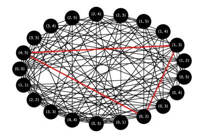
Figure 1: The graph $G$ defined in the main text for $N=6$. The bold colored edges correspond to the clique found by the procedure shown in Fig. 2.

Construction of cliques using the finite projective plane. Our algorithm works when $N=\Pi^{K}+1$ for a prime $\Pi$ and an integer $K>0$. When this is not the case, it suffices to choose the smallest $\Pi^{K}$ larger than $N-1$. We consider a finite projective plane of the order $\Pi^{K}$ as the Desarguesian plane using the finite field $\mathbb{F}_{\Pi^{K}}$ [32]. Below, for simplicity, we restrict ourselves to the case of $K=1$ where the finite field is $\mathbb{Z}_{\Pi}$ and all the arithmetics (addition, multiplication, and their inverse operations) on the elements of the field are those of integers modulo $\Pi$. All the discussion described here apply to the case of arbitrary $K>1$ by considering the corresponding arithmetics on the finite field.

The projective plane is defined by $\mathcal{P}$, a set called points, and $\mathcal{L}$, a family of the subset of $\mathcal{P}$ which is called lines. The set $\mathcal{P}$ consists of three types of points: a single point $P_{\alpha}$, $\Pi$ points $\{P_{\beta}(y)\}_{y=0}^{\Pi-1}$, and $\Pi^{2}$ points $\{P_{\gamma}(x,y)\}_{x,y=0}^{\Pi-1}$. (see also Fig. 2). The lines also consists of three types of the subset of points: $\mathcal{L}=\{L_{\alpha}\}\cup\{L_{\beta}(i)\}_{i=0}^{\Pi-1}\cup\{L_{\gamma}(i,j)\}_{i,j=0}^{\Pi-1}$, defined as

$$\begin{split}L_{\alpha}&=\left\{P_{\alpha},P_{\beta}(0),\ldots,P_{\beta}(\Pi-1)\right\},\\ L_{\beta}(i)&=\left\{P_{\alpha},P_{\gamma}(i,0),\ldots,P_{\gamma}(i,\Pi-1)\right\},\\ L_{\gamma}(i,j)&=\left\{P_{\beta}(i),P_{\gamma}(k,(ik+j)\bmod\Pi)\right\}_{k=0}^{\Pi-1}.\end{split}$$ (19)

The total number of lines is $\Pi^{2}+\Pi+1$. Intuitively, the point $\{P_{\gamma}(x,y)\}$ is interpreted as a two-dimensional plane with coordinates $x,y=0,\cdots,\Pi-1$, and the points $\{P_{\beta}(x)\}$ and $P_{\alpha}$ are points at infinity. $\mathcal{P}$ and $\mathcal{L}$ are known to constitute a finite projective plane. This means that for any two points in $\mathcal{P}$ there exists only one line that contains (passes) both. Also, for any two lines in $\mathcal{L}$, there exists only one point that is contained by both simultaneously.

Our idea to find a edge clique cover of $G$ begins by placing $\Pi+1=N$ points on the plane. Namely, we define $\mathcal{S}=\{S(0),\cdots,S({\Pi})\}$, a subset of $\mathcal{P}$, as (see Fig. 2)

$$S(\Pi)=P_{\alpha},\>S(k)=P_{\gamma}(k,k^{2}\bmod\Pi)\>(k=0,1,\cdots,\Pi-1).$$ (20)

We then associate a line $L_{v}$ of the plane to each vertex $v$ of the graph $G$ as follows. For $v=(l,l)\in V_{1}$ (Eq. (18)), the line $L_{v}$ is defined as the line that passes $S(l)$ and does not pass other points in $\mathcal{S}$. There always exists only one such line on the plane (see Appendix A.2 for proof). For $v=(l,l^{\prime})\in V_{2}$ (Eq. (18)), the line $L_{v}$ is defined as the line that passes both $S(l)$ and $S(l^{\prime})$. The property of the finite projective plane assures the existence and uniqueness of such line. Moreover, distinct vertices are always associated to distinct lines, i.e., $v\neq v^{\prime}\in V\Leftrightarrow L_{v}\neq L_{v^{\prime}}$ holds because there is no line that passes three distinct points in $\mathcal{S}$ [33, 34] (for completeness, we prove this fact in Appendix A.1).

The complementary set of $\mathcal{S}$ in $\mathcal{P}$, $\mathcal{K}:=\mathcal{P}\setminus\mathcal{S}$, consists of $(\Pi^{2}+\Pi+1)-(\Pi+1)=\Pi^{2}$ points. To a given point $p_{k}$ in $\mathcal{K}$ ($k=1,\cdots,\Pi^{2}$), we associate a set of vertices $C_{k}$ defined as,

$$C_{k}:=\{v\in V\>\text{such that {\hbox{L_v}} passes {\hbox{p_k}}}\}.$$ (21)

We claim that $\mathcal{C}_{1},\cdots,\mathcal{C}_{\Pi^{2}}$ are cliques of the graph $G$ and constitute a edge clique cover of $G$.

Proposition 1.

A set $\{C_{k}\}_{k=1}^{\Pi^{2}}$ satisfies the followings:

1. Each $C_{k}$ is a clique of the graph $G$.

2. $\{C_{k}\}_{k=1}^{\Pi^{2}}$ is a edge clique cover of $G$. That is, for any edge between two distinct vertices $v$ and $v^{\prime}$ on the graph $G$, there exists some $C_{k}$ satisfying $v,v^{\prime}\in C_{k}$.

Proof.

To prove (a), consider two distinct vertices $v=(v_{1},v_{2}),v^{\prime}=(v^{\prime}_{1},v^{\prime}_{2})$ in $C_{k}$. Two distinct lines $L_{v},L_{v^{\prime}}$ associated to these vertices intersects at $p_{k}\in\mathcal{K}$ by definition. Suppose that there does not exists an edge between $v$ and $v^{\prime}$. If $v,v^{\prime}\in V_{1}$, the non-existence of the edge implies $v_{1}=v_{2}=v^{\prime}_{1}=v^{\prime}_{2}$, but this contradicts with $v\neq v^{\prime}$. If $v\in V_{1}$ and $v^{\prime}\in V_{2}$, the non-existence of the edge implies $v_{1}=v_{2}=v^{\prime}_{1}\neq v^{\prime}_{2}$ (or $v_{1}=v_{2}=v^{\prime}_{2}\neq v^{\prime}_{1}$) holds and that $L_{v}$ $L_{v^{\prime}}$ intersects at the point $S(v_{1})\in\mathcal{S}$ other than $p_{k}$. This contradicts with the uniqueness of the intersection between two lines. Similarly, if $v,v^{\prime}\in V_{2}$, the non-existence of the edge implies that $L_{v}$ and $L_{v^{\prime}}$ intersects at some point in $\mathcal{S}$ other than $p_{k}$. Again this contradicts with the uniqueness of the intersection between two lines. Therefore, there must exist an edge between $v$ and $v^{\prime}$ on the graph $G$, which proves (a).

To prove (b), let us take an edge between $v$ and $v^{\prime}$ on the graph $G$ (note that $v\neq v^{\prime}$). There are two distinct lines $L_{v}$ and $L_{v^{\prime}}$, and it has exactly one intersection $P\in\mathcal{P}$ on the plane. The point $P$ must be in $\mathcal{K}$ due to the same argument to prove (a). Therefore, there is some $k$ satisfying $p_{k}=P$, and $C_{k}$ contains $v$ and $v^{\prime}$. ∎

Figure 2: The projective plane used in our algorithm for $N=6\>(\Pi=5)$. Grids with different colors correspond to three distinct lines which pass $P_{\gamma}(4,3)$ (the grid filled with black). The darkest gray line passes $S(0)$ and $S(2)$, the next darkest does $S(1)$ and $S(3)$, and the lightest does $S(4)$ and $S(5)$. Therefore, the clique corresponding to $P_{\gamma}(4,3)$ is $C=\{(0,2),(1,3),(4,5)\}$ which is colored in Fig. 1.

Definition of measurement clique. Now that we have a set of pairs of integers $\{C_{k}\}_{k=1}^{\Pi^{2}}$ by using the finite projective plane, which satisfies Eq. (16) and the conditions described there, the measurement clique to evaluate all the terms $\expectationvalue{A_{pq,\sigma}A_{rs,\sigma}}$ and $\expectationvalue{n_{p\sigma}A_{rs,\sigma}}$ for both $\sigma=\uparrow,\downarrow$ can be explicitly constructed by taking $J_{k}=C_{k}$ in Eq. (17). The number of the measurement cliques is $\Pi^{2}=(N-1)^{2}$.

III.2.5 Summary for measurement cliques

To summarize, the measurement cliques we need to evaluate all the terms in the Hamiltonian [Eq. (5)] are

$$\mathbb{U}=\{\mathcal{C}^{\mathrm{part}}\}\cup\mathbb{U}^{[1]}\cup\mathbb{U}^{[2,\mathrm{diff}]}\cup\mathbb{U}^{[2,\mathrm{same}]}.$$ (22)

The number of the total measurement cliques is $1+2(N-1)+(N-1)^{2}+(N-1)^{2}=2N^{2}-2N+1=2N^{2}+O(N)$. The result is summarized in Tab. 1.

III.3 Quantum circuits for measuring operators in cliques

After constructing the measurement cliques, we consider how to measure all the operators $A_{pq,\sigma}$ contained in each measurement clique simultaneously. Strategies for measuring a single $A_{pq,\sigma}$ on a quantum computer depends strongly on the choice of the fermion-to-qubit mapping. However, typical mappings (e.g., Jordan-Winger, parity, or Bravyi-Kitaev; see also [35]) transform fermionic states with the fixed particle number, $\ket{f_{0\uparrow},\cdots,f_{N-1\uparrow},f_{0\downarrow},\cdots,f_{N-1\downarrow}}:=\prod_{p,\sigma}(a_{p\sigma}^{\dagger})^{f_{p\sigma}}\ket{\mathrm{vac}}$ with $f_{p\sigma}=0,1$ and $\ket{\mathrm{vac}}$ being the fermionic vaccum state, into a computational basis state of qubits and thus a particle number operator $n_{p\sigma}$ of fermions into a projection operator on computational basis states. For such cases, measurement of $A_{pq,\sigma}$ reduces to a computational basis measurement after applying a unitary $U_{pq,\sigma}$ such that $U_{pq,\sigma}^{\dagger}A_{pq,\sigma}U_{pq,\sigma}$ can be written by the number operators.

In the language of fermions, $U_{pq,\sigma}$ can, for example, be

$$U_{pq,\sigma}=\exp\left[-\frac{\pi}{4}(a^{\dagger}_{p\sigma}a_{q\sigma}-a^{\dagger}_{q\sigma}a_{p\sigma})\right]$$ (23)

which leads to

$$U_{pq,\sigma}^{\dagger}A_{pq,\sigma}U_{pq,\sigma}=n_{p\sigma}-n_{q\sigma}.$$ (24)

The challenge is how to efficiently implement such $U_{pq,\sigma}$ for all operators in a clique on a quantum computer with possibly limited connectivity. One choice is to use the product of Eq.  (23) for all $A_{pq,\sigma}$ in the clique. The overall unitary in this case becomes a spin-conserving fermionic orbital rotation. It is known that such a rotation can be performed using a depth-$(2N-3)$ quantum circuit on linearly connected qubits under the Jordan-Wigner encoding [36]. This indeed is an efficient strategy, but below we will give even more efficient strategy which uses parallel application of nearest-neighbor fermionic swap gates for at most $N$ times. Our construction is essentially parallel to that of BBO [28].

Suppose that we want to measure $m$ operators in a clique,

$$\mathcal{C}=\{A_{k_{0}k_{1},\sigma_{0}},\cdots,A_{k_{2m-2}k_{2m-1},\sigma_{m-1}}\},$$ (25)

The measurement cliques other than $\mathcal{C}^{\mathrm{part}}$ can be written in this form. The operators in $\mathcal{C}$ can always be reordered in up-then-down order as,

$$\mathcal{C}=\{A_{k_{0}k_{1},\uparrow},\cdots,A_{k_{2m_{\uparrow}-2}k_{2m_{\uparrow}-1},\uparrow},A_{k_{2m_{\uparrow}}k_{2m_{\uparrow}+1},\downarrow},\cdots,A_{k_{2m-2}k_{2m-1},\downarrow}\},$$ (26)

where $m_{\sigma}$ is the number of $\sigma$-spin operators in the clique. For simplicity, we explain the algorithm for the cases where $\mathcal{C}$ contains only $A_{kk^{\prime},\sigma}$ with $k\neq k^{\prime}$. The extension of the algorithm to the cases with $A_{kk,\sigma}$ is straightforward.

Our strategy for measuring the operators in the clique $\mathcal{C}$ consists of two main steps.

1. Apply nearest-neighbor fermionic swap gates [Eq. (29)] to sort the indices of the operators in Eq. (26) into

   $$\{A_{01,\uparrow},\cdots,A_{2m_{\uparrow}-2,2m_{\uparrow}-1,\uparrow},A_{01,\downarrow},\cdots,A_{2m_{\downarrow}-2,2m_{\downarrow}-1,\downarrow}\}.$$ (27)

   The total number of the fermionic swap gates for this sorting is at most $N^{2}$ and the depth (counting a parallel fermionic swaps as one layer) is at most $N$.

2. Transform the operators in Eq. (27) to number operators. For example, this can be done by the parallel application of orbital rotations given in Eq. (23). However, as we will see later, it is not the only choice. By inspecting the concrete forms of $A_{j,j+1,\sigma}$ under specific fermion-qubit mappings, we can design simpler quantum circuits for diagonalizing them. We find that the Bell measurement circuit suffices our purpose for Jordan-Wigner mapping and a single layer of Hadamard gates does for parity and Bravyi-Kitaev mappings.

We explain these two steps in order.

III.3.1 Sorting operators in the clique by fermionic swaps

We want to find a unitary $U^{\mathrm{swap}}$ such that

$$(U^{\mathrm{swap}})^{\dagger}A_{k_{i}k_{j},\sigma}U^{\mathrm{swap}}=A_{ij,\sigma},$$ (28)

which is equivalent to the transformation from Eq. (26) to Eq. (27). To this end, we utilize the fermionic swap gate,

$$f^{\mathrm{swap}}_{ij,\sigma}=1+a^{\dagger}_{i\sigma}a_{j\sigma}+a^{\dagger}_{j\sigma}a_{i\sigma}-a^{\dagger}_{i\sigma}a_{i\sigma}-a^{\dagger}_{j\sigma}a_{j\sigma}$$ (29)

which is a Hermitian and unitary operator, i.e., $(f^{\mathrm{swap}}_{ij,\sigma})^{2}=I$. Its action can be described as

$$f^{\mathrm{swap}}_{ij,\sigma}a_{i\sigma}f^{\mathrm{swap}}_{ij,\sigma}=a_{j\sigma},\>f^{\mathrm{swap}}_{ij,\sigma}a_{j\sigma}f^{\mathrm{swap}}_{ij,\sigma}=a_{i\sigma},\>f^{\mathrm{swap}}_{ij,\sigma}a_{k\tau}f^{\mathrm{swap}}_{ij,\sigma}=a_{k\sigma}\>(k\neq i,j~{}\lor~{}\sigma\neq\tau).$$ (30)

We construct $U^{\mathrm{swap}}$ as a product of $M_{\uparrow}+M_{\downarrow}$ fermionic swap gates $U^{\mathrm{swap}}=U^{\mathrm{swap}}_{\uparrow}U^{\mathrm{swap}}_{\downarrow}$ where $U^{\mathrm{swap}}_{\uparrow}=f^{\mathrm{swap}}_{i_{1}j_{1},\uparrow}\cdots f^{\mathrm{swap}}_{i_{M_{\uparrow}}j_{M_{\uparrow}},\uparrow}$ and $U^{\mathrm{swap}}_{\downarrow}=f^{\mathrm{swap}}_{i_{1}j_{1},\downarrow}\cdots f^{\mathrm{swap}}_{i_{M_{\downarrow}}j_{M_{\downarrow}},\downarrow}$. $U^{\mathrm{swap}}_{\uparrow}$ and $U^{\mathrm{swap}}_{\downarrow}$ can be constructed exactly in the same manner, so we consider how to construct $U^{\mathrm{swap}}_{\uparrow}$ below.

Define the following integers $p_{l}$ for $l=0,1,\cdots,N-1$ as

$$p_{l}=\begin{cases}m&(\text{if there is $m\leq 2m_{\uparrow}-1$ such that $k_{m}=l$})\\ -1&(\text{otherwise})\end{cases}.$$ (31)

which indicates the position of the integer $l$ in the sequence $(k_{0},k_{1},...,k_{2m_{\uparrow}-1})$. $p_{l}=-1$ corresponds to the case where $l$ is not found in the sequence. Note that $p_{l}$ is well-defined and there is one-to-one correspondence between $(k_{0},k_{1},...,k_{2m_{\uparrow}-1})$ and $(p_{0},p_{1},...,p_{N-1})$ because we assume $k_{0},k_{1},\cdots,k_{2m_{\uparrow}-1}$ are mutually different. Applying fermionic swap gate $f_{ij,\uparrow}^{\mathrm{swap}}$ to the operators in the clique $\mathcal{C}$ invokes a change in $p_{l}$ as an exchange between $p_{i}$ and $p_{j}$ and corresponding change in $k$. Therefore, the problem reduces to finding a sequence of swaps for the elements of $p_{l}$ which results in

$$p^{\prime}_{0}=0,p^{\prime}_{1}=1,\cdots,p^{\prime}_{2m_{\uparrow}-1}=2m_{\uparrow}-1,p^{\prime}_{2m_{\uparrow}}=\cdots=p^{\prime}_{N-1}=-1,$$ (32)

because this $p^{\prime}_{l}$ corresponds to

$$k^{\prime}_{0}=0,k^{\prime}_{1}=1,\cdots,k^{\prime}_{2m_{\uparrow}-1}=2m_{\uparrow}-1.$$ (33)

This problem can be solved by applying the odd-even sort algorithm [37] to $p_{l}$. This algorithm first compares the odd adjacent pairs $(p_{1},p_{2}),\cdots,(p_{N-3},p_{N-2})$ and exchanges two components in each pair if necessary. Second, it does the same for the even adjacent pairs $(p_{0},p_{1}),\cdots,(p_{N-2},p_{N-1})$. Each of these steps requires $N/2$ operations at most but they can be executed in parallel. Iterating this process, it successfully sorts the integer with $N$ steps (i.e., with $N/2$ even and $N/2$ odd steps) at most. Hence we can construct $U^{\mathrm{swap}}_{\uparrow}$ by interpreting exchanges in the sort algorithm as the fermionic swap gates. $U^{\mathrm{swap}}_{\downarrow}$ can be constructed in the same manner and can be executed in parallel with $U^{\mathrm{swap}}_{\uparrow}$. Therefore, $U^{\mathrm{swap}}$ in this construction consists of at most $N$ layers of at most $N$ parallel fermionic swap gates.

The actual representation of the femionic swap gate $f_{ij,\sigma}^{\mathrm{swap}}$ on qubits depends on the fermion-qubit mapping, but it becomes typically local when the swap is occurred at adjacent sites, $i=l,j=l+1$ for some integer $l$. To see this, let us first define fermimon operators $\tilde{a}_{j}$ with $j=0,1,\cdots,2N-1$ labeling both the orbital and the spin simultaneously by

$$\tilde{a}_{j}:=\begin{cases}a_{j,\uparrow}&(0\leq j\leq N-1)\\ a_{j-N,\downarrow}&(N\leq j\leq 2N-1)\end{cases}.$$ (34)

This is the so-called up-then-down convention for ordering spin-orbitals. The Jordan-Wigner [30], parity [31], and Bravyi-Kitaev [31] transformation respectively maps $\tilde{a}_{k}$ to

$$\tilde{a}_{j}\to\left\{\begin{array}[]{ll}(X_{k}+iY_{k})Z_{k-1}\cdots Z_{0}/2&\text{(Jordan-Wigner)}\\ \left(Z_{j-1}X_{j}+iY_{j}\right)X_{j+1}\cdots X_{2N}/2&\text{(parity)}\\ \left(Z_{P(j)}X_{j}X_{U(j)}+iZ_{\rho(j)}Y_{j}X_{U(j)}\right)/2&\text{(Bravyi-Kitaev)}\end{array}\right.,$$ (38)

where $U(j)$ is the so-called update set for $j$, $P(j)$ is the parity set for $j$, $\rho(j)=P(j)$ for even $j$, and $\rho(j)=P(j)\setminus F(j)$ for odd $j$ with $F(j)$ being the flip set (see Ref. [38] for the definition of these sets). From the definition of $f_{i,i+1,\sigma}^{\mathrm{swap}}$ (Eq. (29)), $f_{i,i+1,\sigma}^{\mathrm{swap}}$ becomes a two- and three-qubit operator in the Jordan-Wigner and parity mappings, respectively, because the chain of Pauli $Z$ operators and $X$ operators cancels out. For the Bravyi-Kitaev mapping, it becomes a $O(\log N)$-qubit operator since the number of elements in the sets $U(j)$, $P(j)$, $\rho(j)$, and $F(j)$ is $O(\log N)$ [38].

III.3.2 Diagonalizing $A_{j,j+1,\sigma}$ in specific fermion-to-qubit mappings

Let $\tilde{A}_{kk^{\prime}}:=\tilde{a}_{k}^{\dagger}\tilde{a}_{k^{\prime}}+\tilde{a}_{k^{\prime}}^{\dagger}\tilde{a}_{k}$. Note that the sorted clique (Eq. (27)) only contains $\tilde{A}_{2j,2j+1}$ and therefore we only need to consider how to diagonalize them. Under three different fermion-to-qubit mappings, $\tilde{A}_{2j,2j+1}$ becomes

$$\tilde{A}_{2l,2l+1}\to\left\{\begin{array}[]{ll}(X_{2l}X_{2l+1}+Y_{2l}Y_{2l+1})/2&\text{(Jordan-Wigner)}\\ \left(-Z_{2l-1}X_{2l}Z_{2l+1}+X_{2l}\right)/2&\text{(parity)}\\ \left(-Z_{F(2l+1)\setminus\{2l\}}X_{2l}Z_{2l+1}+X_{2l}\right)/2&\text{(Bravyi-Kitaev)}\end{array}\right..$$ (39)

It is easy to see that, for the Jordan-Wigner mapping, we can diagonalize it by applying the Bell measurement circuit to qubits $2j$ and $2j+1$. Also, it can be seen that the set $F(2l+1)\setminus\{2l\}$ contains only odd integers by inspection. This means that, for the parity and Bravyi-Kitaev mappings, the Hadamard gate to all even-site qubits suffices our purpose. The total number of local gates are $O(N)$ and the depth is $O(1)$ in all of three cases.

IV Discussion

We here discuss several points of our study and compare our result with the previous studies.

IV.1 Optimality of the obtained solution

Our construction of cliques for the graph $G$ in Sec. III.2.4 is almost optimal from the viewpoint of the minimal edge clique cover problem. To show this, we give a lower bound to the number of cliques to cover edges of $G$. Consider a subgraph $G^{\prime}$ where we remove all of vertices in $V_{1}$ and corresponding edges in $G$. The number of cliques to cover all edges in $G^{\prime}$ is clearly less than or equal to that of $G$, and it follows that a lower bound for the number of cliques for the edge cover of $G^{\prime}$ is also a lower bound for $G$. First, we claim that a clique in $G^{\prime}$ can have at most $N/2$ vertices and thus $\frac{N}{2}(\frac{N}{2}-1)/2$ edges. This is because there is an edge between two vertices $(p,q)$ and $(r,s)$ in $V_{2}$ if and only if $p,q,r,s$ are mutually different, and thus a clique corresponds to a pairing of $N$ integers. Second, the number of edges in $G^{\prime}$ is $N(N-1)(N-2)(N-3)/8$. To see this, for every tuple of four integers $(p,q,r,s)$ such that $p<q<r<s$, there are three edges each of which connects the vertices $\{(p,q),(r,s)\}$, $\{(p,r),(q,s)\}$, and $\{(p,s),(q,r)\}$ in a graph $G^{\prime}$. The number of combinations of such integers is $\binom{N}{4}$, and therefore the statement follows. Combining these two facts, we conclude that the number of cliques to cover all edges in $G^{\prime}$ must be at least $[N(N-1)(N-2)(N-3)/8]/[\frac{N}{2}(\frac{N}{2}-1)/2]=(N-1)(N-3)$. Therefore, our algorithm, where the number of cliques is $(N-1)^{2}$, provides an optimal solution to the minimal edge clique cover problem of $G$ up to the subleading order terms.

IV.2 Classical computational cost for constructing measurement cliques

The classical computational cost for constructing the measurement cliques in our method is $O(N^{3})$, which comes from creating a set $C_{k}$ in Eq. (21). For each $p_{k}\in\mathcal{K}$ (the number of $k$ is $\Pi^{2}=O(N^{2})$), we add a vertex $v$ on $G$ to $\mathcal{C}_{k}$ by inspecting the line passing $p_{k}$ and $S(i)$ (the total number of $i$ is $\Pi+1=N$): when the line passes $S(i)$ and $S(j)$, we add $(i,j)$ or $(j,i)$ to $\mathcal{C}_{k}$, and when the line passes only $S(i)$, we add $(i,i)$ to $\mathcal{C}_{k}$. Note that this computational cost is optimal when we seek to find $O(N^{2})$ measurement cliques, because the output of the algorithm must be of size $O(N^{3})$ by the discussion in Sec. IV.1.

This $O(N^{3})$ scaling of the classical computational cost is much smaller than the methods to create the measurement clique consisting of the terms of the Hamiltonian as is [16, 17, 18, 19, 20, 21, 22, 23, 24]. In those methods, one should calculate the commutativity or anti-commutativity of pairs of the $O(N^{4})$ terms in the Hamiltonian, which results in as huge as $O(N^{8})$ classical computational cost. The target problem of the application of quantum computers in quantum chemistry lies for more than $N\sim 50$, and such scaling can be problematic in practice.

IV.3 Comparison of the number of measurement cliques in our algorithm with that of previous studies

Our algorithm can determine the expectation value of the quantum chemistry Hamiltonian with $O(N^{2})$ measurement cliques. Again, this is advantageous over the conventional methods to create the measurement cliques consisting of the terms of the Hamiltonian [16, 17, 18, 19, 20, 21, 22, 23, 24], in which the total number of the measurement cliques is $O(N^{3})$ [22, 24].

Let us compare our algorithm with BBO algorithm [28]. The fermionic 1,2-RDMs are defined as

$$\rho^{[1]}_{pq}=\expectationvalue{\tilde{a}_{p}^{\dagger}\tilde{a}_{q}},\rho^{[2]}_{pqrs}=\expectationvalue{\tilde{a}_{p}^{\dagger}\tilde{a}_{q}^{\dagger}\tilde{a}_{r}\tilde{a}_{s}}.$$ (40)

for mutually distinct integers $p,q,r,s=0,\cdots,2N-1$. BBO algorithm can determine the fermionic 2-RDM with $O(N^{2})$ measurement clique, so the scaling is the same as ours. It is based on the Majorana representation of the fermions and constructs measurement cliques of the Majorana operators by considering sets of integers similar to Eq. (16). That is, the products of two Majorana operators, rather than the products of four Majorana operators, consist the measurement cliques to evaluate the fermionic 2-RDM (represented as products of four Majorana operators). The authors (BBO) [28, 29] claimed that the number of measurement cliques to evaluate the fermionic 2-RDM is

$$4N^{2}\left(\frac{16}{3}4^{-N_{\mathrm{sym}}}+2^{1-N_{\mathrm{sym}}}\right),$$ (41)

where $N_{\mathrm{sym}}$ is the number of Pauli operators $W$ such that $[H,W]=0$. For general Hamiltonians for quantum chemistry calculation [Eq. (1)], typically we have two such symmetries: the numbers of spin-up and spin-down electrons [39]. Putting $N_{\mathrm{sym}}=2$ in the above equation yields

$$4N^{2}\left(\frac{16}{3}4^{-2}+2^{-1}\right)=\frac{10}{3}N^{2},$$ (42)

which is slightly larger than our method, $2N^{2}$. We note that our method determines only the “symmetric part” of the fermionic 2-RDM,

$$\expectationvalue{\tilde{A}_{pq}\tilde{A}_{rs}}=\rho^{[2]}_{pqrs}+\rho^{[2]}_{qprs}+\rho^{[2]}_{pqsr}+\rho^{[2]}_{qpsr},$$ (43)

which is sufficient to determine the expectation value of the molecular Hamiltonian [Eq. (1)] with the symmetries (4). In contrast, BBO algorithm evaluates all elements of the fermionic 2-RDM.

V Summary and outlook

In this study, we have proposed a measurement scheme for general molecular Hamiltonians in quantum chemistry [Eq. (1)]. We have used the symmetries of the coefficients in the Hamiltonian and reduced the problem of evaluating the expectation value of the Hamiltonian into the evaluation of the terms $\expectationvalue{A_{pq,\sigma}}$ and $\expectationvalue{A_{pq,\sigma}A_{rs,\tau}}$. We have classified all the possible terms appearing in the Hamiltonian and proposed a measurement clique for each type of the terms. Especially, the measurement cliques for the terms $\expectationvalue{A_{pq,\sigma}A_{rs,\sigma}}$ with mutually-different $p,q,r,s$ have been constructed by finding the edge clique cover of the specific graph using the novel method based on the finite projective plane. The total number of the distinct measurement cliques (or measurement circuits) is $2N^{2}+O(N)$ with $2N$ being the number of spin orbitals (fermions), which exhibits better scaling compared with the previous method (BBO algorithm). We have shown explicit quantum circuits to measure operators in the measurement cliques, and those circuits consist of $O(N^{2})$ one- or two-qubit gates with depth $O(N)$ for Jordan-Wigner and parity mappings. Evaluation of the expectation value of the Hamiltonian is one of the most fundamental subroutines among various algorithms for the applications of quantum computers to quantum chemistry, so our method can be utilized in broad studies on quantum algorithms.

As future work, it is intriguing to apply the proposed method to actual Hamiltonians in quantum chemistry and numerically investigate a standard deviation of the estimated energy expectation value with using our measurement cliques. Another interesting direction is to generalize our method using the finite projective plane to higher order fermionic RDMs, such as $\expectationvalue{\tilde{a}_{p}^{\dagger}\tilde{a}_{q}^{\dagger}\tilde{a}_{r}^{\dagger}a_{s}a_{t}a_{u}}$.

*

Appendix A Proof for several properties of points $\mathcal{S}$ on finite projective plane

In this Appendix, we prove several properties of points $\mathcal{S}$ on the finite projective plane described in Sec. III.2.4.

A.1 Three points in $\mathcal{S}$ never appear on a single line

We prove the following:

Lemma 1.

Three distinct points in $S$ never appear on a single line.

Proof.

From the definition of $L_{\alpha}$, there is a single point $S(\Pi)=P_{\alpha}$ on $L_{\alpha}$. Similarly, $L_{\beta}(i)$ has only two points $S(\Pi)=P_{\alpha}$ and $S(i)=P_{\gamma}(i,i^{2}\mod\Pi)$ in $\mathcal{S}$. For $L_{\gamma}(i,j)$, suppose that $L_{\gamma}(i,j)$ has three distinct points $S(a)$, $S(b)$ and $S(c)$ in $S$. This implies

$$a^{2}\equiv ia+j\mod\Pi,\>b^{2}\equiv ib+j\mod\Pi.$$ (44)

Subtracting them results in

$$a^{2}-b^{2}\equiv i(a-b)\mod\Pi.$$ (45)

By using the assumption $a\neq b$, we reach

$$a+b\equiv i\mod\Pi.$$ (46)

Similarly, we can show

$$a+c\equiv i\mod\Pi.$$ (47)

by using the assumption $a\neq c$. These two equations (46)(47) lead to $b=c$, but this contradicts with the assumption that three points $S(a),S(b)$ and $S(c)$ are distinct. ∎

A.2 There is only one line that passes a point in $\mathcal{S}$

We prove the following property,

Lemma 2.

For any $S(k)\in\mathcal{S}$, there is only one line that passes $S(k)$ and does not pass any other points in $\mathcal{S}$.

Proof.

For $S(\Pi)=P_{\alpha}$, $L_{\alpha},L_{\beta}(0),\cdots,L_{\beta}(\Pi-1)$ are the only lines passing $S(\Pi)$ . Among these lines, only the line $L_{\alpha}$ passes $S(\Pi)$ and does not pass any other points in $\mathcal{S}$. For $S(k)=P_{\gamma}(k,k^{2}\mod\Pi)$ with $k=0,\cdots,\Pi-1$, $L_{\beta}(k)$ and $L_{\gamma}(a,k^{2}-ak\mod\Pi)$ for $a=0,\cdots,\Pi-1$ are the only lines passing $S(k)$. The line $L_{\beta}(k)$ passes two points in $\mathcal{S}$, namely, $S(k)$ and $S(\Pi)=P_{\alpha}$. For $l=0,\cdots,k-1,k+1,\cdots,\Pi-1$, the line $L_{\gamma}(k+l,k^{2}-(k+l)k\mod\Pi)$ passes the point $S(l)=P_{\gamma}(l,l^{2}\mod\Pi)$ as well as $S(k)$. We show that the remaining line $L_{\gamma}(2k,k^{2}-2k\cdot k\mod\Pi)=L_{\gamma}(2k,-k^{2}\mod\Pi)$ do not pass the points in $\mathcal{S}$ other than $S(k)$ as follows. Suppose that $L_{\gamma}(2k,-k^{2}\mod\Pi)$ passes $S(m)=P_{\gamma}(m,m^{2}\mod\Pi)$ for $S(m)\neq S(k)$. Then we have

$$m^{2}\equiv 2km-k^{2}\mod\Pi\>\Leftrightarrow\>(m-k)^{2}\equiv 0\mod\Pi.$$ (48)

Since $\Pi$ is a prime, this means $m\equiv k\mod\Pi$. This contradicts with $S(k)\neq S(m)$. ∎

References

- McArdle et al. [2020] S. McArdle, S. Endo, A. Aspuru-Guzik, S. C. Benjamin, and X. Yuan, Quantum computational chemistry, Rev. Mod. Phys. 92, 015003 (2020).
- Cao et al. [2019] Y. Cao, J. Romero, J. P. Olson, M. Degroote, P. D. Johnson, M. Kieferová, I. D. Kivlichan, T. Menke, B. Peropadre, N. P. D. Sawaya, S. Sim, L. Veis, and A. Aspuru-Guzik, Quantum chemistry in the age of quantum computing, Chem. Rev., Chem. Rev. 119, 10856 (2019).
- Peruzzo et al. [2014] A. Peruzzo, J. McClean, P. Shadbolt, M.-H. Yung, X.-Q. Zhou, P. J. Love, A. Aspuru-Guzik, and J. L. O’Brien, A variational eigenvalue solver on a photonic quantum processor, Nature Communications 5, 4213 (2014).
- Tilly et al. [2022] J. Tilly, H. Chen, S. Cao, D. Picozzi, K. Setia, Y. Li, E. Grant, L. Wossnig, I. Rungger, G. H. Booth, and J. Tennyson, The Variational Quantum Eigensolver: A review of methods and best practices, Physics Reports 986, 1 (2022).
- Preskill [2018] J. Preskill, Quantum Computing in the NISQ era and beyond, Quantum 2, 79 (2018).
- Kitaev [1995] A. Y. Kitaev, Quantum measurements and the abelian stabilizer problem, arXiv:quant-ph/9511026v1 [quant-ph] (1995).
- Cleve et al. [1998] R. Cleve, A. Ekert, C. Macchiavello, and M. Mosca, Quantum algorithms revisited, Proc. R. Soc. London, Ser. A 454, 339 (1998).
- O’Brien et al. [2021] T. E. O’Brien, M. Streif, N. C. Rubin, R. Santagati, Y. Su, W. J. Huggins, J. J. Goings, N. Moll, E. Kyoseva, M. Degroote, C. S. Tautermann, J. Lee, D. W. Berry, N. Wiebe, and R. Babbush, Efficient quantum computation of molecular forces and other energy gradients, arXiv:2111.12437v2 [quant-ph] (2021).
- Huggins et al. [2022] W. J. Huggins, K. Wan, J. McClean, T. E. O’Brien, N. Wiebe, and R. Babbush, Nearly optimal quantum algorithm for estimating multiple expectation values, Phys. Rev. Lett. 129, 240501 (2022).
- Ibe et al. [2022] Y. Ibe, Y. O. Nakagawa, N. Earnest, T. Yamamoto, K. Mitarai, Q. Gao, and T. Kobayashi, Calculating transition amplitudes by variational quantum deflation, Phys. Rev. Res. 4, 013173 (2022).
- Mitarai et al. [2022] K. Mitarai, K. Toyoizumi, and W. Mizukami, Perturbation theory with quantum signal processing, arXiv:2210.00718v2 [quant-ph] (2022).
- Gonthier et al. [2022] J. F. Gonthier, M. D. Radin, C. Buda, E. J. Doskocil, C. M. Abuan, and J. Romero, Measurements as a roadblock to near-term practical quantum advantage in chemistry: resource analysis, Phys. Rev. Research 4, 033154 (2022).
- Mizukami et al. [2020] W. Mizukami, K. Mitarai, Y. O. Nakagawa, T. Yamamoto, T. Yan, and Y.-y. Ohnishi, Orbital optimized unitary coupled cluster theory for quantum computer, Phys. Rev. Research 2, 033421 (2020).
- Takeshita et al. [2020] T. Takeshita, N. C. Rubin, Z. Jiang, E. Lee, R. Babbush, and J. R. McClean, Increasing the representation accuracy of quantum simulations of chemistry without extra quantum resources, Phys. Rev. X 10, 011004 (2020).
- Sokolov et al. [2020] I. O. Sokolov, P. K. Barkoutsos, P. J. Ollitrault, D. Greenberg, J. Rice, M. Pistoia, and I. Tavernelli, Quantum orbital-optimized unitary coupled cluster methods in the strongly correlated regime: Can quantum algorithms outperform their classical equivalents?, J. Chem. Phys. 152, 124107 (2020).
- McClean et al. [2016] J. R. McClean, J. Romero, R. Babbush, and A. Aspuru-Guzik, The theory of variational hybrid quantum-classical algorithms, New J. Phys. 18, 023023 (2016).
- Kandala et al. [2017] A. Kandala, A. Mezzacapo, K. Temme, M. Takita, M. Brink, J. M. Chow, and J. M. Gambetta, Hardware-efficient variational quantum eigensolver for small molecules and quantum magnets, Nature 549, 242 (2017).
- Jena et al. [2019] A. Jena, S. Genin, and M. Mosca, Pauli partitioning with respect to gate sets, arXiv preprint arXiv:1907.07859 10.48550/ARXIV.1907.07859 (2019).
- Izmaylov et al. [2020] A. F. Izmaylov, T.-C. Yen, R. A. Lang, and V. Verteletskyi, Unitary partitioning approach to the measurement problem in the variational quantum eigensolver method, Journal of Chemical Theory and Computation 16, 190 (2020).
- Verteletskyi et al. [2020] V. Verteletskyi, T.-C. Yen, and A. F. Izmaylov, Measurement optimization in the variational quantum eigensolver using a minimum clique cover, The Journal of Chemical Physics 152, 124114 (2020).
- Yen et al. [2020] T.-C. Yen, V. Verteletskyi, and A. F. Izmaylov, Measuring all compatible operators in one series of single-qubit measurements using unitary transformations, Journal of Chemical Theory and Computation 16, 2400 (2020).
- Gokhale et al. [2020] P. Gokhale, O. Angiuli, Y. Ding, K. Gui, T. Tomesh, M. Suchara, M. Martonosi, and F. T. Chong, measurement cost for variational quantum eigensolver on molecular hamiltonians, IEEE Transactions on Quantum Engineering 1, 1 (2020).
- Hamamura and Imamichi [2020] I. Hamamura and T. Imamichi, Efficient evaluation of quantum observables using entangled measurements, npj Quantum Information 6, 56 (2020).
- Zhao et al. [2020] A. Zhao, A. Tranter, W. M. Kirby, S. F. Ung, A. Miyake, and P. J. Love, Measurement reduction in variational quantum algorithms, Phys. Rev. A 101, 062322 (2020).
- Crawford et al. [2021] O. Crawford, B. van Straaten, D. Wang, T. Parks, E. Campbell, and S. Brierley, Efficient quantum measurement of Pauli operators in the presence of finite sampling error, Quantum 5, 385 (2021).
- Huggins et al. [2021] W. J. Huggins, J. R. McClean, N. C. Rubin, Z. Jiang, N. Wiebe, K. B. Whaley, and R. Babbush, Efficient and noise resilient measurements for quantum chemistry on near-term quantum computers, npj Quantum Information 7, 23 (2021).
- Yen and Izmaylov [2021] T.-C. Yen and A. F. Izmaylov, Cartan subalgebra approach to efficient measurements of quantum observables, PRX Quantum 2, 040320 (2021).
- Bonet-Monroig et al. [2020] X. Bonet-Monroig, R. Babbush, and T. E. O’Brien, Nearly optimal measurement scheduling for partial tomography of quantum states, Phys. Rev. X 10, 031064 (2020).
- [29] T. E. O’Brien, private communication, Eq. (6) in [28] should be instead of the one in the paper, .
- Jordan and Wigner [1928] P. Jordan and E. Wigner, Über das paulische äquivalenzverbot, Zeitschrift für Physik 47, 631 (1928).
- Bravyi and Kitaev [2002] S. B. Bravyi and A. Y. Kitaev, Fermionic quantum computation, Annals of Physics 298, 210 (2002).
- Albert and Sandler [2014] A. Albert and R. Sandler, An Introduction to Finite Projective Planes, Dover Books on Mathematics (Dover Publications, 2014).
- Segre [1955] B. Segre, Ovals in a finite projective plane, Canadian Journal of Mathematics 7, 414–416 (1955).
- Browne et al. [2023] P. J. Browne, S. T. Dougherty, and P. O. Catháin, Segre’s theorem on ovals in desarguesian projective planes, arXiv:2301.05171v1 [math.CO] (2023).
- Steudtner and Wehner [2018] M. Steudtner and S. Wehner, Fermion-to-qubit mappings with varying resource requirements for quantum simulation, New Journal of Physics 20, 063010 (2018).
- Kivlichan et al. [2018] I. D. Kivlichan, J. McClean, N. Wiebe, C. Gidney, A. Aspuru-Guzik, G. K.-L. Chan, and R. Babbush, Quantum simulation of electronic structure with linear depth and connectivity, Phys. Rev. Lett. 120, 110501 (2018).
- Habermann [1972] N. Habermann, Parallel Neighbor-Sort (or the Glory of the Induction Principle), Tech. Rep. AD-759-248 (Carnegie Mellon University, 1972).
- Seeley et al. [2012] J. T. Seeley, M. J. Richard, and P. J. Love, The bravyi-kitaev transformation for quantum computation of electronic structure, The Journal of Chemical Physics 137, 224109 (2012).
- Bravyi et al. [2017] S. Bravyi, J. M. Gambetta, A. Mezzacapo, and K. Temme, Tapering off qubits to simulate fermionic hamiltonians, arXiv:1701.08213v1 [quant-ph] (2017).